4/12/2010

1

GG450

April 13, 2010

Seismic Reflection III Data Processing

Today’s material comes from p. 163-198 in the text book.

Please read and understand all of this material!

Reflection Processing We've been talking about acquisition of reflection data - spreads, frequency and resolution considerations, etc. Now we talk about how these data are processed to obtain reasonable profiles of the sub-surface "geology". Purpose: To enhance the reflection record so that noise is minimized and desired reflections are enhanced, and corrected to provide the clearest possible representation of the structures below.

Reflection Processing

Step 1: Resample To make sure that we do not alias our data during the acquisition phase, we usually use a higher sample rate than necessary. For instance, marine data is usually sampled at 2 msec interval (500 Hz), so the Nyquist frequency is 250 Hz, which is MUCH higher than the actual frequency content of our source, so we resample the data to 4 msec samples (250 Hz). In case there may be some signal above Nyquist, we must first use an antialias filter to remove all signals above the Nyquist frequency. Why would we want to resample our data?

Reflection Processing

Step 2: Noise reduction Our field shot records often have noise in them. What might cause noise in land field records? Marine field records? We need to filter the noise from the field data before continuing our processing

Raw shot gather with lots of noise

4/12/2010

2

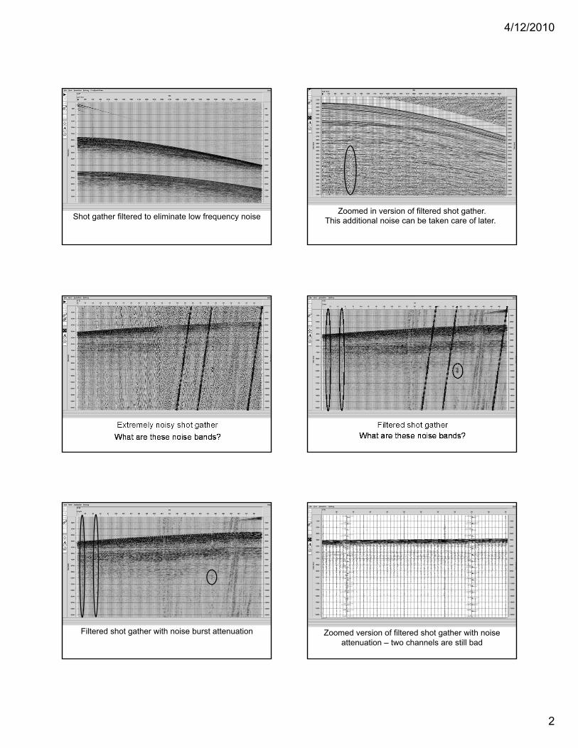
Shot gather filtered to eliminate low frequency noise Zoomed in version of filtered shot gather.

This additional noise can be taken care of later.

Extremely noisy shot gather Filtered shot gather

Filtered shot gather with noise burst attenuation Zoomed version of filtered shot gather with noise attenuation – two channels are still bad

4/12/2010

3

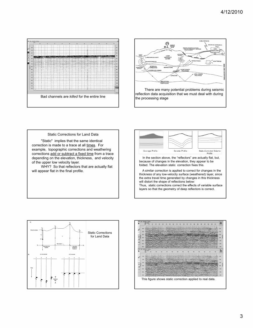
Bad channels are killed for the entire line

There are many potential problems during seismic reflection data acquisition that we must deal with during the processing stage

Static Corrections for Land Data

"Static" implies that the same identical correction is made to a trace at all times. For example, topographic corrections and weathering corrections add or subtract a fixed time from a trace depending on the elevation, thickness, and velocity of the upper low velocity layer. WHY? So that reflectors that are actually flat will appear flat in the final profile.

In the section above, the “reflectors” are actually flat, but, because of changes in the elevation, they appear to be folded. The elevation static correction fixes this.

A similar correction is applied to correct for changes in the thickness of any low-velocity surface (weathered) layer, since the extra travel time generated by changes in this thickness will distort the shape of reflections below: Thus, static corrections correct the effects of variable surface layers so that the geometry of deep reflectors is correct.

Static Corrections for Land Data

This figure shows static correction applied to real data.

4/12/2010

4

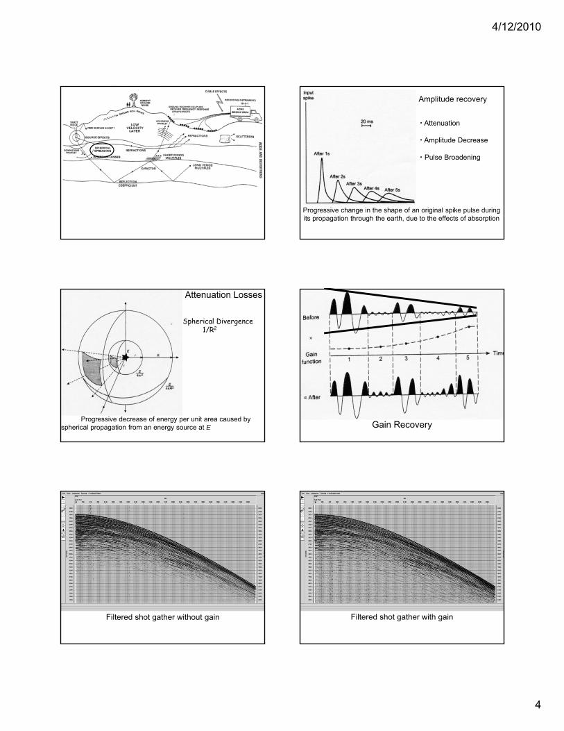
• Attenuation • Amplitude Decrease • Pulse Broadening

Amplitude recovery

Progressive change in the shape of an original spike pulse during its propagation through the earth, due to the effects of absorption

Spherical Divergence 1/R2

Attenuation Losses

Progressive decrease of energy per unit area caused by spherical propagation from an energy source at E Gain Recovery

Filtered shot gather without gain Filtered shot gather with gain

4/12/2010

5

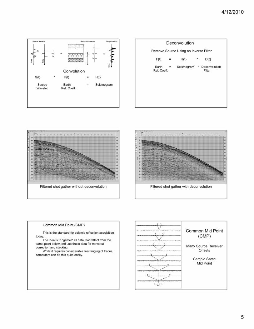
Convolution

G(t) * F(t) = H(t) Source Earth = Seismogram Wavelet Ref. Coeff.

Deconvolution

Remove Source Using an Inverse Filter

F(t) = H(t) * D(t) Earth = Seismogram * Deconvolution Ref. Coeff. Filter

Filtered shot gather without deconvolution Filtered shot gather with deconvolution

Common Mid Point (CMP) This is the standard for seismic reflection acquisition

today. The idea is to "gather" all data that reflect from the

same point below and use these data for moveout correction and stacking.

While it requires considerable rearranging of traces, computers can do this quite easily.

Common Mid Point (CMP)

Many Source Receiver

Offsets

Sample Same Mid Point

4/12/2010

6

31

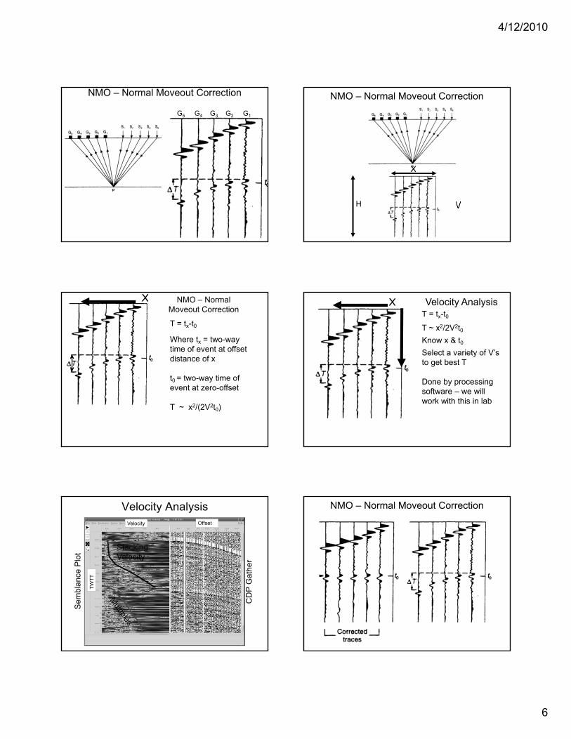
NMO – Normal Moveout Correction

G5 G4 G3 G2 G1

NMO – Normal Moveout Correction

H V

X

T = tx-t0

Where tx = two-way time of event at offset distance of x t0 = two-way time of event at zero-offset T ~ x2/(2V2t0)

X NMO – Normal Moveout Correction

Velocity Analysis T = tx-t0

T ~ x2/2V2t0

Know x & t0

Select a variety of V’s to get best T Done by processing software – we will work with this in lab

X

Velocity Analysis

Sem

blan

ce P

lot

CD

P G

athe

r

Velocity Offset

TW

TT

NMO – Normal Moveout Correction

4/12/2010

7

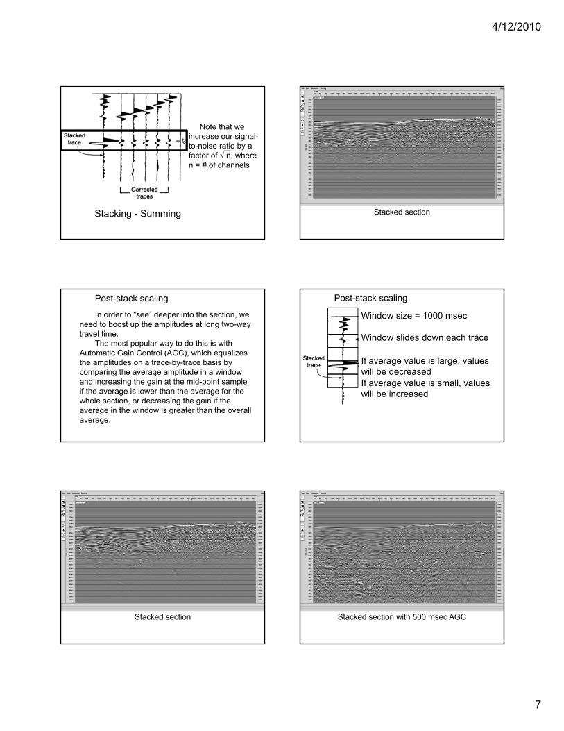
Stacking - Summing

Note that we increase our signal-to-noise ratio by a factor of √ n, where n = # of channels

Stacked section

Post-stack scaling

In order to “see” deeper into the section, we need to boost up the amplitudes at long two-way travel time.

The most popular way to do this is with Automatic Gain Control (AGC), which equalizes the amplitudes on a trace-by-trace basis by comparing the average amplitude in a window and increasing the gain at the mid-point sample if the average is lower than the average for the whole section, or decreasing the gain if the average in the window is greater than the overall average.

Post-stack scaling

Window size = 1000 msec Window slides down each trace If average value is large, values will be decreased

If average value is small, values will be increased

Stacked section Stacked section with 500 msec AGC