GG313 Lecture 3

8/30/05

Identifying trends, error analysis

Significant digits

Homework review

• Are the trends different?• What are the trends in mm/year?• Waikiki is ~2 m above sea level. How long

before it is flooded?• Discuss your results. Are the data adequate

for this study? Is noise a problem?• Are there any other trends that correlate

between the two data sets?

Removing non-linear trends

Procedure

1) Take Log(y) of the data and plot

2) If line concave, try y-n

Log(A y-n)=Log(A) - n Log(y)

1) If convex, try yn

OR….

Plot Log x vs Log y

Log(A y-n)=Log(A) - n Log(y)

If Log (x)=Log(A) - n Log(y)

Then our data will plot as a straight line with a slope equal to n.

So, if we get the best LINEAR fit to the log-log data, we can solve for A and n.

SHOW EXCEL PLOTS

Note that the log curve is not linear - why??

Bottom Line:

ALWAYS plot your data before analysis

ERROR ANALYSIS

Error analysis is the study of uncertainties in measurement of continuous data. Discrete data may have no uncertainty.

Errors are NOT mistakes. You cannot avoid them by being careful, but you can minimize them by using the best methods and equipment available. All instruments have uncertainties in their measurements; you need to know what they are.

Reporting Uncertainties

In most situations, you, as a scientist are obligated to report reasonable estimates of possible errors in your results. While unpleasant, this usually isn’t too difficult.

For example, if you take a measurement that comes out to be 101 units, and you are sure that it can’t be smaller than 100 or larger than 102, then you could report the result as 101±1.

Alternatively, (and often better) you could use the fractional uncertainty x/|xbest| where x is 1 in this example and xbest is 101. Fractional uncertainty is expressed as a percentage: 101±1%.

Significant Figures

In general, the least significant digit in a number should be the same order of magnitude as the uncertainty in that number.

Carry all available digits through calculations, but only report significant digits.

Example:

You calculate a volume as 3.21624 ±.5 m3.

You should REPORT this number as 3.2 ±.5 m3.

Uncertainties in derived quantities

Consider two measurements, , that will be combined to form new parameters. How do we determine the new uncertainties for the following situations:

€

x ± δx and y ± δy

€

s = x + y

d = x − y

p = x ⋅ y

q = x / y

For the sum, the largest likely value is:

€

smax = x + δx + y + δy

And the smallest is:

€

smin = x −δx + y −δy

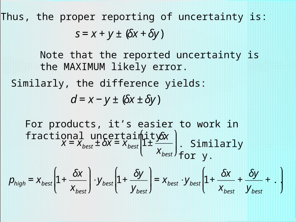
Thus, the proper reporting of uncertainty is:

€

s = x + y ± (δx + δy).

Note that the reported uncertainty is the MAXIMUM likely error.

Similarly, the difference yields:

€

d = x − y ± (δx ± δy).

For products, it’s easier to work in fractional uncertainity:

€

x = xbest ± δx = xbest 1±δx

xbest

⎛

⎝ ⎜

⎞

⎠ ⎟. Similarly for y.

€

phigh = xbest 1+δx

xbest

⎛

⎝ ⎜

⎞

⎠ ⎟⋅ ybest 1+

δy

ybest

⎛

⎝ ⎜

⎞

⎠ ⎟= xbest ⋅ ybest 1+

δx

xbest+δy

ybest+ ...

⎛

⎝ ⎜

⎞

⎠ ⎟

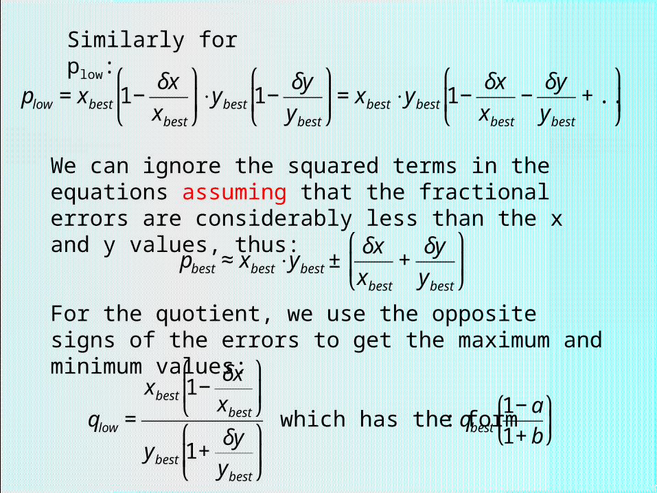
Similarly for plow:

€

plow = xbest 1−δx

xbest

⎛

⎝ ⎜

⎞

⎠ ⎟⋅ ybest 1−

δy

ybest

⎛

⎝ ⎜

⎞

⎠ ⎟= xbest ⋅ ybest 1−

δx

xbest−δy

ybest+ ...

⎛

⎝ ⎜

⎞

⎠ ⎟

We can ignore the squared terms in the equations assuming that the fractional errors are considerably less than the x and y values, thus:

€

pbest ≈ xbest ⋅ ybest ±δx

xbest+δy

ybest

⎛

⎝ ⎜

⎞

⎠ ⎟

For the quotient, we use the opposite signs of the errors to get the maximum and minimum values:

€

qlow =

xbest 1−δx

xbest

⎛

⎝ ⎜

⎞

⎠ ⎟

ybest 1+δy

ybest

⎛

⎝ ⎜

⎞

⎠ ⎟

which has the form: qbest1− a

1+ b

⎛

⎝ ⎜

⎞

⎠ ⎟

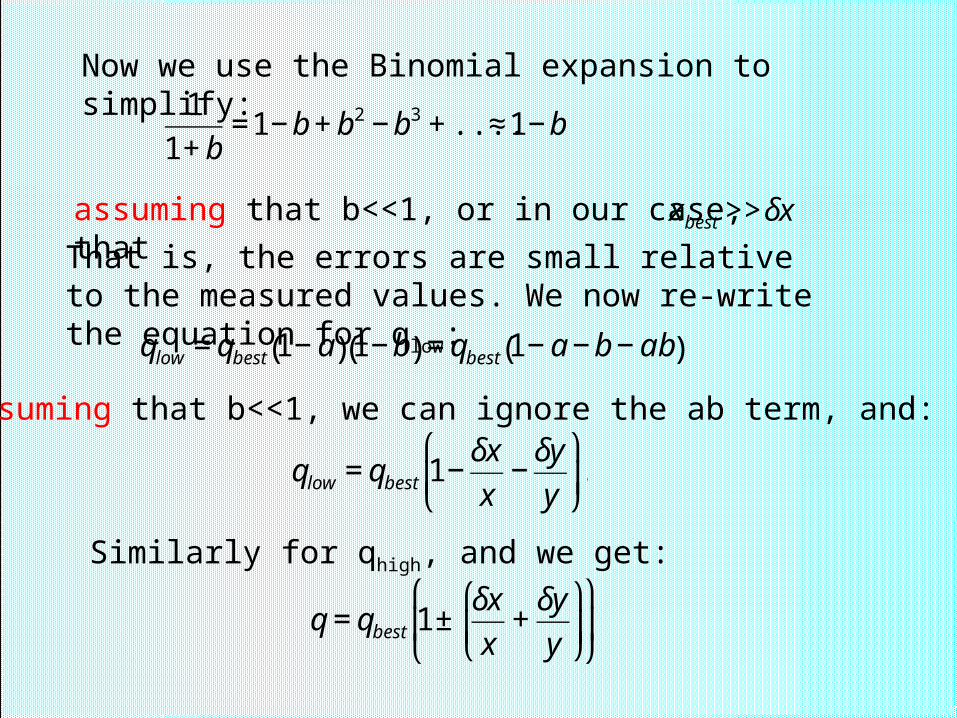
Now we use the Binomial expansion to simplify:

€

1

1+ b=1−b+ b2 −b3 + .... ≈1−b

assuming that b<<1, or in our case, that

€

xbest >>δx

That is, the errors are small relative to the measured values. We now re-write the equation for qlow:

€

qlow = qbest 1− a( ) 1−b( ) = qbest 1− a−b− ab( )

assuming that b<<1, we can ignore the ab term, and:

€

qlow = qbest 1−δx

x−δy

y

⎛

⎝ ⎜

⎞

⎠ ⎟.

Similarly for qhigh, and we get:

€

q = qbest 1±δx

x+δy

y

⎛

⎝ ⎜

⎞

⎠ ⎟

⎛

⎝ ⎜

⎞

⎠ ⎟.

The values above are correct, but they give the MAXIMUM likely error, not the MOST likely error. So they overstate the errors in many situations.

If our data are independent and randomly distributed about a mean value, then better values for the Most likely error are given by (shown later):

€

s = δd = δx( )2

+ δy( )2

and

€

p = δq =δx

x

⎛

⎝ ⎜

⎞

⎠ ⎟2

+δy

y

⎛

⎝ ⎜

⎞

⎠ ⎟

2

If we have the case s=nx, s=n x since the values of not independent.

If we have the case p=xn, then the fractional uncertainties will be:

€

pp

= nδx

x

See Wessel’s notes Eqns 1.26-1.29 (page 11) for more.

The red words above highlight assumptions. Two assumptions were made depending on the situation, one being that the errors are small relative to the measured values, HOW SMALL IS SMALL?

The 2nd that the measurements are randomly distributed and independent. If these assumptions do NOT hold, then we must take care not to make them!

0

0.1

0.2

0.3

0.4

0.5

0.6

0.7

0.8

0.9

1

0 0.1 0.2 0.3 0.4 0.5 0.6 0.7 0.8 0.9 1

1/(1+b)

1-b

error

If b is 0.1, the error using only the first term of the binomial expansion is ~11%

Examples:

x=250±5, y=10±2

What are s, d, p, and q with no assumptions of independence?

If x and y are independent, what are s, d, p, and q?

We expect that the minimum change in gravity as we move over a particular region to be 0.1 mGals, where 1 Gal=1 cm/s^2. The acceleration of gravity is about 980 Gals, or 980,000 mgals. What sort of measurement errors are required to have a resolution of 0.01 mGal?

Our gravity meter must detect changes of 1 part in 98000000, or 1 part in 10-8.

We’re offered a pendulum to use to make our measurements, where the equation for the period of the pendulum is:

€

g =4π 2l

T 2

⎛

⎝ ⎜

⎞

⎠ ⎟

Where g=gravity, l is the pendulum length, and T is the measured period of the pendulum.

Looking at the errors:

€

gg

=δl

l

⎛

⎝ ⎜

⎞

⎠ ⎟2

+ 2δT

T

⎛

⎝ ⎜

⎞

⎠ ⎟2

If l=92.95±0.1 cm and in a test run T=1.936±.004 s,

then:

€

g =4π 2l

T 2

⎛

⎝ ⎜

⎞

⎠ ⎟= 4π 292.95 /1.9362 = 9.79035m /s2

And our errors are:

€

gg

=δl

l

⎛

⎝ ⎜

⎞

⎠ ⎟2

+ 2δT

T

⎛

⎝ ⎜

⎞

⎠ ⎟2

=0.1

92.95

⎛

⎝ ⎜

⎞

⎠ ⎟2

+ 20.004

1.936

⎛

⎝ ⎜

⎞

⎠ ⎟2

≈ 0.4%

Can we use this for our field work?

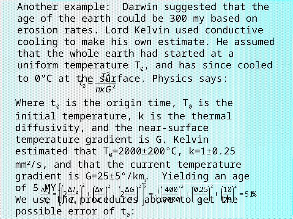
Another example: Darwin suggested that the age of the earth could be 300 my based on erosion rates. Lord Kelvin used conductive cooling to make his own estimate. He assumed that the whole earth had started at a uniform temperature T0, and has since cooled to 0°C at the surface. Physics says:

€

t0 =T0

2

πκG2

Where t0 is the origin time, T0 is the initial temperature, k is the thermal diffusivity, and the near-surface temperature gradient is G. Kelvin estimated that T0=2000±200°C, k=1±0.25 mm2/s, and that the current temperature gradient is G=25±5°/km. Yielding an age of 5 MY.We use the procedures above to get the possible error of t0:

€

Δt0t0

= 2ΔT0

T0

⎛

⎝ ⎜

⎞

⎠ ⎟

2

+Δκ

κ

⎛

⎝ ⎜

⎞

⎠ ⎟2

+ 2ΔG

G

⎛

⎝ ⎜

⎞

⎠ ⎟2 ⎡

⎣ ⎢ ⎢

⎤

⎦ ⎥ ⎥

1

2

=400

2000

⎛

⎝ ⎜

⎞

⎠ ⎟2

+0.25

1

⎛

⎝ ⎜

⎞

⎠ ⎟2

+10

25

⎛

⎝ ⎜

⎞

⎠ ⎟2

= 51%

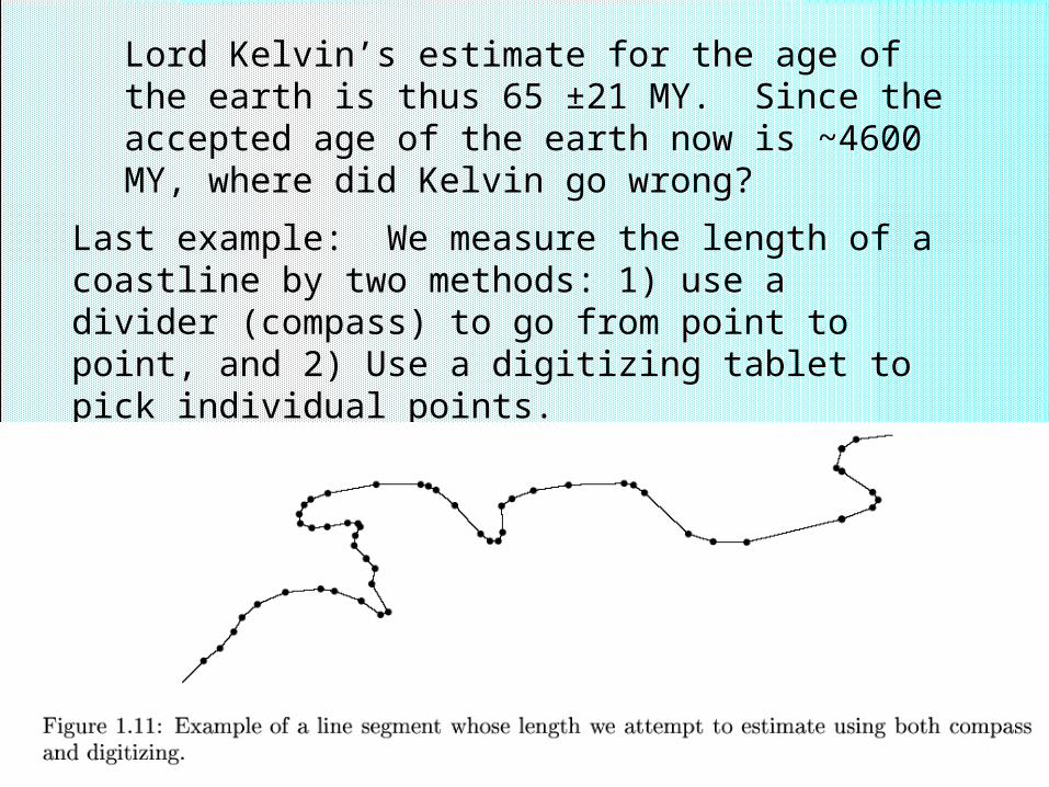
Lord Kelvin’s estimate for the age of the earth is thus 65 ±21 MY. Since the accepted age of the earth now is ~4600 MY, where did Kelvin go wrong?

Last example: We measure the length of a coastline by two methods: 1) use a divider (compass) to go from point to point, and 2) Use a digitizing tablet to pick individual points.

For case 1) we set the dividers to an opening of Δx=1±.025 cm and march along the line counting the number of increments.

For case 2) we sample the line about every cm, Δx=1±.1 cm.

Assume it takes about 50 steps to do the whole shoreline, or about 50 cm.

What are the uncertainties of the two methods?

The errors accumulate very differently. For case 1) the measurements are NOT INDEPENDENT, while for case 2) they are. For case 1) l=N 0.025 cm=1.25 cm

For case 2) l=N 0.025 cm=1.25 cm only the end points are uncertain, so l=√(2*0.12) cm=0.14 cm

Uncertainties in Functions

Let’s say we measure an angle and want to take the cosine of that angle. What are the uncertainties of the cosine based on our measurement?

We have y=f(x) where we measure x. The uncertainty in y (y) is then the tangent to the function at x times the uncertaintly in x, IF x is small relative to x :

€

y =df

dx xδx

Example: y=cos(x), x=20°±3°

€

y =dcos(x)

dx x= 20°

π

180°

⎛

⎝ ⎜

⎞

⎠ ⎟3° = −sin(20°)

3π

180°= 0.02

So, y=cos(x)=0.94 ±0.02

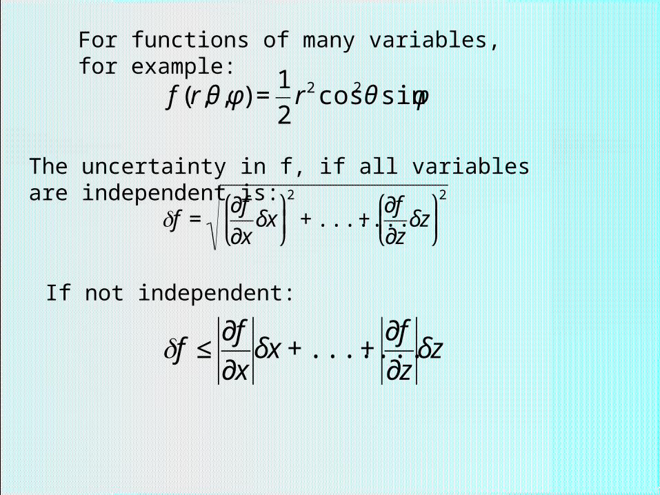
For functions of many variables, for example:

€

f (r,θ,φ) =1

2r2 cos2θ sinφ

The uncertainty in f, if all variables are independent is:

€

f =∂f

∂xδx

⎛

⎝ ⎜

⎞

⎠ ⎟2

+ .......+∂f

∂zδz

⎛

⎝ ⎜

⎞

⎠ ⎟2

If not independent:

€

f ≤∂f

∂xδx + .......+

∂f

∂zδz

€

f (r,θ,φ) =1

2r2 cos2θ sinφ

Example using the spherical function:

We measure r=10±0.1, =60±1°, and =10±1°. Assuming independence, the uncertainty in f will then be:

€

f = rcos2θ sinφδr( )2

+ r2 cosθ sinθ sinφδθ( )2 1

2r2 cos2θ cosφδφ

⎛

⎝ ⎜

⎞

⎠ ⎟2

Which evaluates to: f(r, , ) =2.17±0.26

NEXT CLASS: PROBABILITY BASICS

TODAY - NOW Chris Conger thesis defense POST 723