Germán Sierra

IFT@UAM-CSIC

in collaboration with

P.K. Townsend and J. Rodríguez-Laguna

1st-i-Link workshop, Macro-from-Micro: Quantum Gravity and Cosmology,

24-27 June 2013, CSIC, Madrid

Riemann hypothesis (1859):

the complex zeros of the zeta function

all have real part equal to 1/2

€

ς sn( ) = 0, sn ∈ C → sn =1

2+ i En, En ∈ ℜ, n ∈ Z€

ς(s)

Polya and Hilbert conjecture (circa 1910):

There exists a self-adjoint operator H whose discrete spectra is given by the imaginary part of the Riemann zeros,

€

H ψ n = En ψ n ⇒ En ∈ ℜ ⇒ RH : True

The problem is to find H: the Riemann operator

This is known as the spectral approach to the RH

Richard DawkingHis girlfriend?

Outline

• The Riemann zeta function• Hints for the spectral interpretation • H = xp model by Berry-Keating and Connes• Landau version of the Connes’s xp model • Analogue of Hawking radiation (M. Stone) • The xp model à la Berry-Keating revisited• Extended xp models and their spacetime interpretation• Xp and Dirac fermion in Rindler space • Contact with Riemann zeta

Based on:

“Landau levels and Riemann zeros” (with P-K. Townsend) Phys. Rev. Lett. 2008

“A quantum mechanical model of the Riemann zeros” New J. of Physics 2008

”The H=xp model revisited and the Riemann zeros”, (with J. Rodriguez-Laguna) Phys. Rev. Lett. 2011

”General covariant xp models and the Riemann zeros” J. Phys. A: Math. Theor. 2012

”An xp model on AdS2 spacetime” (with J. Molina-Vilaplana)arXiv:1212.2436.

€

ς(s) =1

n s, Re s >1

1

∞

∑

Zeta(s) can be written in three different “languages”

Sum over the integers (Euler)

Product over primes (Euler)

€

ς(s) =1

1− p−s, Re s >1

p= 2,3,5,K

∏

Product over the zeros (Riemann)

€

ς(s) =π s / 2

2(s −1)Γ(1+ s /2)1−

s

ρ

⎛

⎝ ⎜

⎞

⎠ ⎟

ρ

∏

Importance of RH: imposes a limit to the chaotic behaviour of the primes

If RH is true then “there is music in the primes” (M. Berry)

The number of Riemann zeros in the box

€

0 < Re s <1, 0 < Ims < E

is given by

€

NR (E) = N(E) + N fl (E)

N(E) ≈E

2πlog

E

2π−1

⎛

⎝ ⎜

⎞

⎠ ⎟+

7

8+ O(E−1)

N fl (E) =1

πArgς (

1

2+ i E) = O(log E)

Smooth(E>>1)

Fluctuation

Riemann function

€

ξ(s) ≡ π −s / 2 Γs

2

⎛

⎝ ⎜

⎞

⎠ ⎟ς(s)

€

ξ 1

2− iE

⎛

⎝ ⎜

⎞

⎠ ⎟=ξ

1

2+ iE

⎛

⎝ ⎜

⎞

⎠ ⎟

- Entire function- Vanishes only at the Riemann zeros- Functional relation

€

ξ

€

ξ(s) =ξ(1 − s)

Sketch of Riemann’s proof

Jacobi theta function

Modular transformation

Support for a spectral interpretation of the Riemann zeros

Selberg’s trace formula (50´s): Classical-quantum correspondence similar to formulas in number theory

Montgomery-Odlyzko law (70´s-80´s): The Riemann zeros behave as the eigenvalues of the GUE in Random Matrix Theory -> H breaks time reversal

Berry´s quantum chaos proposal (80´s-90´s): The Riemann operator is the quantization of a classical chaotic Hamiltonian

Berry-Keating/Connes (99): H = xp could be the Riemann operator

Berry´s quantum chaos proposal (80´s-90´s): the Riemann zeros are spectra of a quantum chaotic system

Analogy between the number theory formula:

€

N fl (E) = −1

π

1

m pm / 2sin m E log p( )

m=1

∞

∑p

∑

and the fluctuation part of the spectrum of a classical chaotic Hamiltonian

€

N fl (E) =1

π

1

m2sinh(mλα /2)sin m E Tα( )

m =1

∞

∑α

∑

Dictionary:

€

Periodic trayectory (α ) ↔ prime number (p)

Period (Tα ) ↔ log p

Idea: prime numbers are “time” and Riemann zeros are “energies”

• In 1999 Berry and Keating proposed that the 1D classical Hamiltonian H = x p, when properly quantized, may contain the Riemann zeros in the spectrum

• The Berry-Keating proposal was parallel to Connes adelic approach to the RH.

These approaches are semiclassical (heuristic)

The classical trayectories are hyperbolae in phase space

€

x(t) = x0 e t , p(t) = p0 e−t , E = x0 p0

Time Reversal Symmetry is broken ( )

€

x → x, p → −p

The classical H = xp model

Unboundedtrayectories

Berry-Keating regularization

Planck cell in phase space:

€

x > l x, p >l p , h = l x l p = 2π (h =1)

Number of semiclassical states

Agrees with number of zeros asymptotically (smooth part)

€

Nsc (E) ≈E

2πlog

E

2π−

E

2π+

7

8

Connes regularization

Cutoffs in phase space:

€

x < Λ, p < Λ

Number of semiclassical states

As spectrum = continuum - Riemann zeros

€

Λ→ ∞€

Nsc (E) ≈E

2πlog

Λ2

2π−

E

2πlog

E

2π+

E

2π

Are there quantum versions of the Berry-

Keating/Connes “semiclassical” models?

Are there quantum versions of the Berry-

Keating/Connes “semiclassical” models?

- Quantize H = xp

- Quantize Connes xp model

-Quantize Berry-Keating model

Continuum spectrum

Landau model

Rindler space

Hawking radiation

Define the normal ordered operator in the half-line

€

H0 =1

2(x ˆ p + ˆ p x) = −i(x

d

dx+

1

2)

€

φE (x) =1

x1/ 2−i E

H is a self-adjoint operator: eigenfunctions

The spectrum is a continuum

€

E ∈(−∞,∞)

€

0 < x < ∞

Quantization of H = xp

On the real line H is doubly degenerate with even and oddeigenfunctions under parity

€

φE+(x) =

1

x1/ 2−i E , φE

− (x) =sign(x)

x1/ 2−i E

Lagrangian of a 2D charge particle in a uniform magnetic field Bin the gauge A = B (0,x):

€

L =μ

2

dx

dt

⎛

⎝ ⎜

⎞

⎠ ⎟2

+dy

dt

⎛

⎝ ⎜

⎞

⎠ ⎟2 ⎡

⎣ ⎢

⎤

⎦ ⎥−

e B

c

dy

dtx

Classically, the particle follows cyclotronic orbits:

€

ωc =e B

μ c

Cyclotronic frequency:

QM: Landau levels

€

En = hωc n +1

2

⎛

⎝ ⎜

⎞

⎠ ⎟, n = 0,1,K

Highly degenerate

Wave functions of the Lowest Landau Level n=0 (LLL)

€

ψ(x, y) =1

π 1/ 4 Ly1/ 2

e i ky y e−(x−ky )2 / 2

€

Lx ×Ly

Degeneracy

€

NL =Lx Ly

2π l 2= NΦ

€

l =hc

e B: magnetic length

€

LLLL = pdx

dt− HLLL ⇒ HLLL = 0

Effective Hamiltonian of the LLL

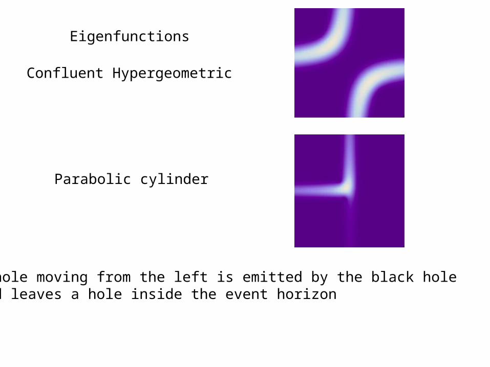
Projection to the LLL is obtained in the limit

€

ωc → ∞ ⇔ μ → 0

€

L =μ

2

dx

dt

⎛

⎝ ⎜

⎞

⎠ ⎟2

+dy

dt

⎛

⎝ ⎜

⎞

⎠ ⎟2 ⎡

⎣ ⎢

⎤

⎦ ⎥−

e B

c

dy

dtx → LLLL = −

e B

c

dy

dtx

Define

€

p =h y

l 2→ LLLL = p

dx

dt

In the quantum model

€

x, p[ ] = i h

Degeneracy of LLL

Add an electrostatic potential xy

Normal modes: cyclotronic and hyperbolic

€

ωc =e B

μ ccoshϑ , ωh = i

e B

μ csinhϑ sinh(2ϑ ) =

2λμc 2

e B2

⎛

⎝ ⎜

⎞

⎠ ⎟

€

L =μ

2

dx

dt

⎛

⎝ ⎜

⎞

⎠ ⎟2

+dy

dt

⎛

⎝ ⎜

⎞

⎠ ⎟2 ⎡

⎣ ⎢

⎤

⎦ ⎥−

e B

c

dy

dtx − e λ x y

(with P.K. Townsend)

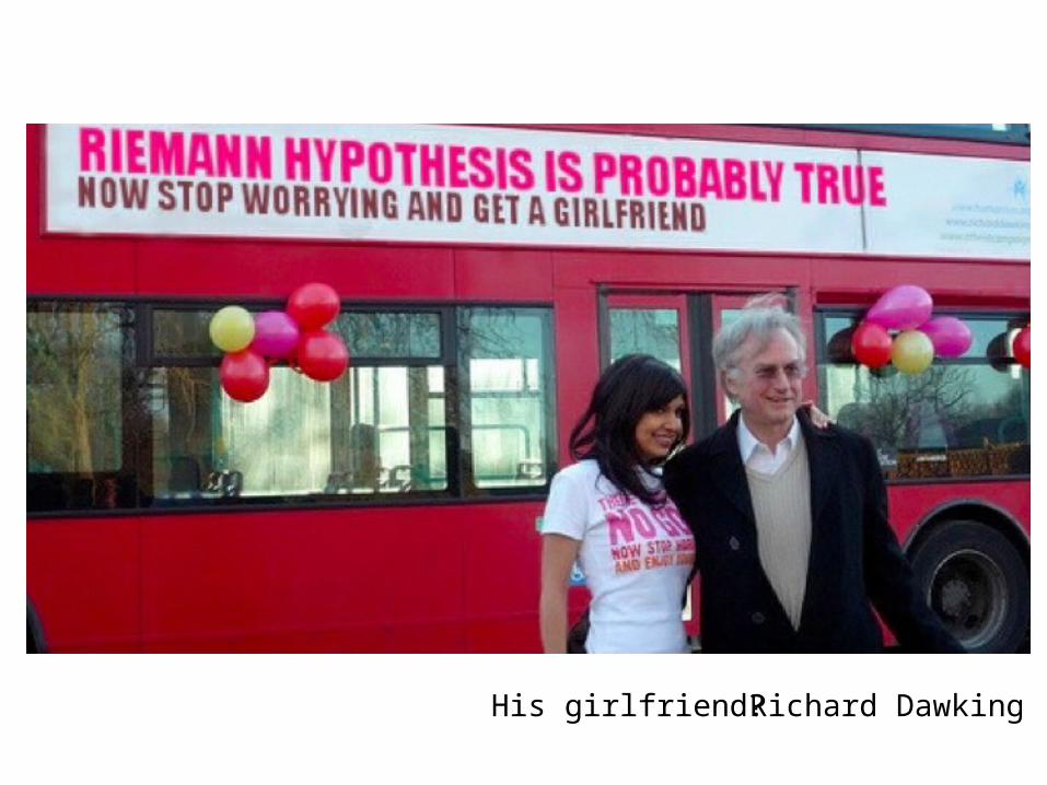
In the limit

€

ωc >> ωh

Effective Lagrangian:

€

LLLL = pdx

dt− ωh x p

only the lowest Landau level is relevant

€

ωc ≈e B

μ c, ωh ≈ i

λ c

B

Effective Hamiltonian

€

HLLL = ωh x p

Quantum derivation of Connes semiclassical result

€

H =1

2μpx

2 + py +h

l 2x

⎛

⎝ ⎜

⎞

⎠ ⎟2 ⎡

⎣ ⎢

⎤

⎦ ⎥+ e λ x y

€

ωc >> ωhIn the limit the eigenfunctions are confluent hypergeometric fns

€

φE+(x,y)∝ e−x 2 / 2l 2

M1

4+

i E

2,1

2,(x − i y)2

2l 2

⎛

⎝ ⎜

⎞

⎠ ⎟

φE− (x,y)∝(x − i y) e−x 2 / 2l 2

M3

4+

i E

2,3

2,(x − i y)2

2l 2

⎛

⎝ ⎜

⎞

⎠ ⎟

even

odd

Matching condition on the boundaries (even functions)

€

φE+(x,L) =e i L x / l 2

φE+(L, x) →

Γ1

4+

i E

2

⎛

⎝ ⎜

⎞

⎠ ⎟

Γ1

4−

i E

2

⎛

⎝ ⎜

⎞

⎠ ⎟

L2

2l 2

⎛

⎝ ⎜

⎞

⎠ ⎟

−i E

=1

Taking the log

In agreement with the Connes formula

€

N(E) =E

2πlog

L2

2πl 2+1− N(E)

For odd functions 1/4 -> 3/4

Problem with Connes xp

- Spectrum becomes a continuum in the large size limit

- No real connection with Riemann zeros

Go back to Berry-Keating version of xp and try to make it quantum

An analogue of Hawking radiation in the Quantum Hall Effect

2DEG

€

V = λ x y

Hall fluid at filling fraction 1with an edge at x=0

There is a horizon generated by

edge

€

vedge =λ

eBy

Velocity at the edge

In the limit proyect to the LLL

€

ωc >> ωh

M. Stone 2012

Edge excitations are described by a chiral 1+1 Dirac fermion

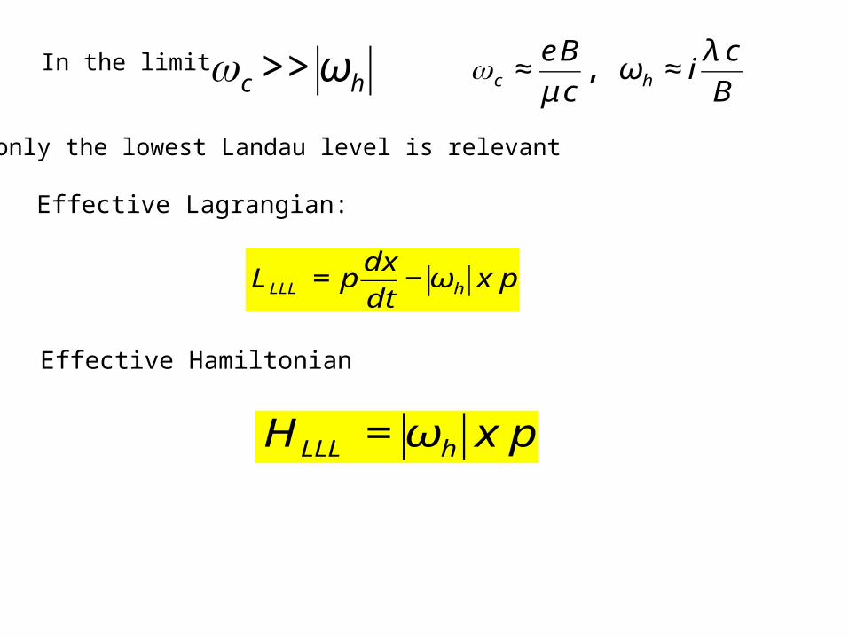
Eigenfunctions

Confluent Hypergeometric

Parabolic cylinder

A hole moving from the left is emitted by the black holeand leaves a hole inside the event horizon

Probability of an outgoing particle or hole is thermal

Corresponds to a Hawking temperature

with a surface gravity given by the edge-velocity acceleration

€

H = x p +l p

2

p

⎛

⎝ ⎜

⎞

⎠ ⎟, x ≥ l x

(with J. Rodriguez-Laguna 2011)

Classical trayectories arebounded and periodic

xp trajectory

€

l x

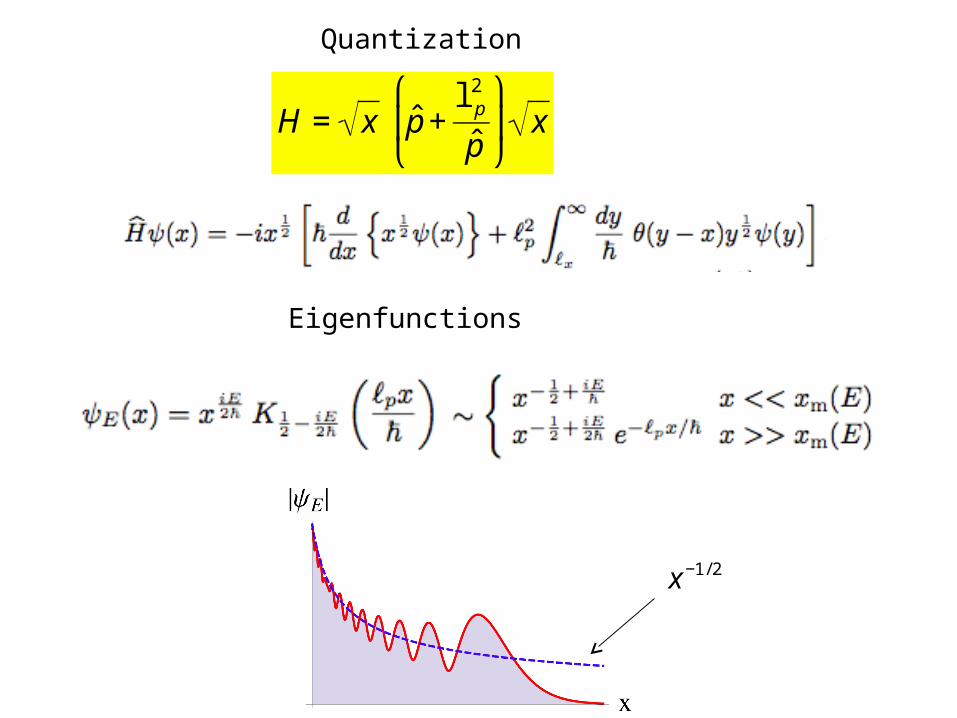
Quantization

€

H = x ˆ p +l p

2

ˆ p

⎛

⎝ ⎜

⎞

⎠ ⎟ x

Eigenfunctions

€

x −1/ 2

H is selfadjoint acting on the wave functions satisfying

Which yields the eq. for the eigenvalues

€

ϑ =0 ↔ En, − En , E0 = 0

ϑ = π ↔ En, − En , E0 ≠ 0

parameter of the self-adjoint extension

Riemann zeros also appear in pairs and 0 is not a zero, i.e

€

ς(1/2) ≠ 0

€

ϑ =π

€

ϑ

Periodic

Antiperiodic

In the limit

€

E /l x l p >>1

€

n(E) ≈E

2π hlog

E

l x l p

−1 ⎛

⎝ ⎜ ⎜

⎞

⎠ ⎟ ⎟+

1

2+ O(1/ E)

€

l x l p = 2π h

€

n(E) ≈E

2π hlog

E

2π h−1

⎛

⎝ ⎜

⎞

⎠ ⎟+

1

2+ O(1/ E)

Not 7/8

First two termsin Riemann formula

Berry-Keating modification of xp (2011)

€

H = x +l x

2

x

⎛

⎝ ⎜

⎞

⎠ ⎟ p +

l p2

p

⎛

⎝ ⎜

⎞

⎠ ⎟, x ≥ 0

€

ˆ H = x +l x

2

x

⎛

⎝ ⎜

⎞

⎠ ⎟

1/ 2

ˆ p +l p

2

ˆ p

⎛

⎝ ⎜

⎞

⎠ ⎟ x +

l x2

x

⎛

⎝ ⎜

⎞

⎠ ⎟

1/ 2

xp =cte

Same as Riemann but the 7/8 is also missing

We are not claiming that our hamiltonian H has an

immediate connection with the Riemann zeta function.

This is ruled out not only by the fact that the mean eigenvalue

density differs from the density of Riemann zeros after the first

terms, but by a more fundamental difference in the periodic

orbits.

For H, there is a single primitive periodic orbit for each energy

E; and for the conjectured dynamics underlying the zeta

function, there is a family of primitive orbits for each ‘energy’ t,

labelled by primes p, with periods log p.

This absence of connection with the primes is shared by all

variants of xp.

Concluding remarks in Berry- Keating paper

“All variants” of the xp model

GS 2012

General covariance: dynamics of a massive particle moving ina spacetime with a metric given by U and V

€

l p = maction:

metric:

curvature:

€

H = x p +l p

2

p

⎛

⎝ ⎜

⎞

⎠ ⎟→U = V = x →R(x) = 0 : spacetime is flat

Change of variables to Minkowsky metric

€

ds2 = ημν dx μ dxν

spacetime region

€

x ≥ l x, − ∞ < t <∞

€

l x

Rindler coordinates

€

ρ ≥l x, − ∞ < φ < ∞

Boundary : accelerated observer with

€

a =1/l x

€

U

€

ds2 = dρ 2 −ρ 2 dφ2

x 0 = ρ sinhφ, x1 = ρ coshφ

Dirac fermion in Rindler space (GS work in progress)

Solutions of Dirac equation

Boundary conditions

Reproduces the eq. for the eigenvalues

Lessons:

- xp model can be formulated as a relativistic field theoryof a massive Dirac fermion in a domain of Rindler spacetime

is the mass and is the acceleration of the boundary

- energies agree with the first two terms of Riemann formula provided

€

1/l x

€

l p

€

l xl p = 2π h

Where is the zeta function?

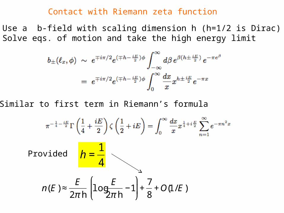
Contact with Riemann zeta function

Use a b-field with scaling dimension h (h=1/2 is Dirac)Solve eqs. of motion and take the high energy limit

Similar to first term in Riemann’s formula

Provided

€

h =1

4

€

n(E) ≈E

2π hlog

E

2π h−1

⎛

⎝ ⎜

⎞

⎠ ⎟+

7

8+ O(1/ E)

Boundary condition on B

Riemann zeros as spectrum !!

• The xp model is a promissing candidate to yield a spectral interpretation of the Riemann zeros

• Connes xp -> Landau xy model -> Analogue of Hawking radiation in the FQHE (Stone). No connection with Riemann zeros.

• Berry-Keating xp -> Dirac fermion in Rindler space

• Conjecture: b-c field theory in Rindler space with some additional ingredient may yield the final answer

• Where are the prime numbers in this construction?

• Is there a connection between Quantum Gravity and Number theory?

Thanks for your attention