Credit and Banking in a DSGE Model

of the Euro Area

Andrea Gerali Stefano Neri Luca Sessa Federico M. Signoretti∗

May 11, 2009

Abstract

This paper studies the role of credit-supply factors in business cycle fluctuations. Tothis end, an imperfectly competitive banking sector is introduced into a DGSE modelwith financial frictions. Banks issue loans to both households and firms, obtainfunding via deposits and accumulate capital out of retained earnings. Marginscharged on loans depend on bank capital-to-asset ratio and on the degree of interestrate stickiness. Bank balance-sheet constraints establish a link between the businesscycle, which affects bank profits and thus capital, and the supply and the cost ofloans. The model is estimated with Bayesian techniques using data for the euroarea. We show that shocks originating in the banking sector explain the largestfraction of the fall of output in 2008 in the euro area, while macroeconomic shocksplayed a smaller role. We also find that an unexpected reduction in bank capital canhave a substantial impact on the real economy and particularly on investment.

JEL: E30; E32; E43; E51; E52;

Keywords: Collateral Constraints; Banks; Banking Capital; Sticky Interest Rates.

∗Banca d’Italia, Research Department. The opinions expressed here are those of the authors onlyand do not necessarily reflect the view of the Banca d’Italia. Email: andrea.gerali@bancaditalia.it; ste-fano.neri@bancaditalia.it; luca.sessa@bancaditalia.it; federicomaria.signoretti@bancaditalia.it. We ben-efited of useful discussions with Tobias Adrian, Vasco Curdia, Jordi Galı, Eugenio Gaiotti, LeonardoGambacorta, Matteo Iacoviello, John Leahy, Jesper Linde, Fabio Panetta, Anti Ripatti, Argia Sbordoneand Mike Woodford. We also thanks participants at the Bank of Italy June ’08 “DSGE in the PolicyEnvironment” conference, the Macro Modeling Workshop ’08, the WGEM and CCBS July ’08 Workshopat the Bank of England, the “Financial Markets and Monetary Policy” December ’08 conference at theEuropean Central Bank and at the NY Federal Reserve seminar series.

1 Introduction

Policymakers have often highlighted the importance of financial factors in shaping the

business cycle: the possible interactions between credit markets and the real economy are

a customary part of the overall assessment on the policy stance. Since the onset of the

financial turmoil in August 2007, banks have come again under the spotlight, as losses from

subprime credit exposure and from significant write-offs on asset-backed securities raised

concerns that a wave of widespread credit restrictions might trigger a severe economic

downturn. Credit standard for firms and households were tightened considerably both

in the US and the euro area (Figure 1) as suggested by the Senior Loan Officer Survey

of the Federal Reserve and the Bank Lending Survey of the Eurosystem. Past episodes

like the U.S. Great Depression, the Savings and Loans crises again in the U.S. in the

1980s or the prolonged recession in Finland and Japan in the 1990s stand as compelling

empirical evidence that the banking sector can considerably affect the developments of

the real economy.1

Despite this relevance for policy-making, most workhorse general equilibrium models

routinely employed in academia and policy institutions to study the dynamics of the

main macroeconomic variables generally lack any interaction between financial and credit

markets, on the one hand, and the rest of the economy, on the other. The introduction

of financial frictions in a dynamic general equilibrium (DSGE) framework by Bernanke,

Gertler and Gilchrist (1999) and Iacoviello (2005) has started to fill this gap by intro-

ducing credit and collateral requirements and by studying how macroeconomic shocks

are transmitted or amplified in the presence of these financial elements. These models

assume that credit transactions take place through the market and do not assign any role

to financial intermediaries such as banks.

But in reality banks play a very influential role in modern financial systems, and

especially in the euro area. In 2006, bank deposits in the euro area accounted for more

than three-quarters of household short-term financial wealth, while loans equaled around

90 per cent of total households liabilities (ECB, 2008); similarly, for firms, bank lending

accounted for almost 90 per cent of total corporate debt liabilities in 2005 (ECB, 2007).

Thus, the effective cost/return that private agents in the euro area face when taking their

borrowing/saving decisions are well approximated by the level of banks’ interest rates on

loans and deposits.

1 Awareness seemed to be widespread among economists and policy-makers well before the financialturmoil burst out. For example, in a speech at the “The Credit Channel of Monetary Policy in theTwenty-first Century”Conference held on 15 June 2007 at the Federal Reserve Bank of Atlanta, chairmanBernanke stated that “...Just as a healthy financial system promotes growth, adverse financial conditionsmay prevent an economy from reaching its potential. A weak banking system grappling with nonperformingloans and insufficient capital, or firms whose creditworthiness has eroded because of high leverage ordeclining asset values, are examples of financial conditions that could undermine growth”.

2

In this paper we introduce a banking sector in a DSGE model in order to understand

the role of banking intermediation in the transmission of monetary impulses and to ana-

lyze how shocks that originate in credit markets are transmitted to the real economy. We

are not the first to do this. Recently there has been increasing interest in introducing a

banking sector in dynamic models and to analyze economies where a plurality of financial

assets, differing in their returns, are available to agents (Christiano et al., 2007, and Good-

friend and McCallum, 2007). But in these cases banks operate under perfect competition

and do not set interest rates. We think that a crucial element in modeling banks sector

consists in recognizing them a degree of monopolistic power (in both the deposits and the

loans markets). This allows us to model their interest rate setting behavior and hence also

the different speeds at which banks interest rates adjust to changing conditions in money

market interest rates. Empirical evidence shows that bank rates are indeed heterogeneous

in this respect, with deposit rates adjusting somewhat slower than rates on households

loans, and those in turn slower than rates on firms loans (Kok Sorensen and Werner, 2006

and de Bondt, 2005). On the other hand, compliance to Basel Accords imposes capital

requirements to exert banking activity. We therefore enrich a standard model, featuring

credit frictions and borrowing constraints as in Iacoviello (2005), and a set of real and

nominal frictions as in Christiano et al. (2005) and Smets and Wouters (2003) with an

imperfectly competitive banking sector that collects deposits and then, subject to the

requirement of using banking capital as an input, supplies loans to the private sector.

These banks set different rates for households and firms, applying a time-varying and

slowly adjusting mark-up over the marginal cost of loan production, which includes the

interbank rate and the cost of equity. Loan demand is constrained by the value of housing

collateral for households and capital for entrepreneurs. Banks obtain funding either by

tapping the interbank market at a rate set by the monetary authority or by collecting

deposits from patient households, at a rate set by the banks themselves with a mark-down

over the interbank rate.

We estimate the model with Bayesian techniques and data for the euro area over the

period 1999-2008. The model is used to understand the role of banks and imperfect

competition in the banking sector in the transmission mechanism of monetary policy and

technology shocks. We use it to quantify the contribution of shocks originating within

the banking sector to the slowdown in economic activity during 2008 and to study the

consequences of tightening of credit conditions induced by a reduction in bank capital.

The analysis delivers the following results. First, while financial frictions amplify the

effects of monetary policy compared to a standard new keynesian model, sticky bank rates

dampen (attenuator effect) the effects on the economy that work through a change in the

real rate or in the value of the collateral. Second, shocks in the banking sector explain the

largest fraction of the fall output in 2008 in the euro area while macroeconomic shocks

played a smaller role. Finally, shocks to credit supply can have substantial effects on

3

the economy and particularly on investment. A fall in bank capital forces bank to raise

interest rates resulting in lower demand for loans by households and firms who are forced

to cut on consumption and expenditure.

The rest of the paper is organized as follows. Section 2 describes the model. Section

3 presents the results of the estimation of the model. Section 4 studies the dynamic

properties of the model focusing on monetary policy and technology shocks. Section 5

quantifies the role of shocks originating in the banking sector in the downturn in economic

activity in the euro area during 2008 and studies the effects of a fall in bank capital on

the economy. Section 6 offers some concluding remarks.

2 The model

The economy is populated by two types of households and by entrepreneurs. Households

consume, work and accumulate housing (in fixed supply), while entrepreneurs produce

an homogenous intermediate good using capital bought from capital-good producers and

labor supplied by households. Agents differ in their degree of impatience, i.e. in the

discount factor they apply to the stream of future utility.

Two types of one-period financial instruments, supplied by banks, are available to

agents: saving assets (deposits) and loans. When taking on a bank loan, agents face

a borrowing constraint, tied to the value of tomorrow collateral holdings: households

can borrow against their stock of housing, while entrepreneurs’ borrowing capacity is

tied to the value of their physical capital. The heterogeneity in agents’ discount factors

determines positive financial flows in equilibrium: patient households purchase a posi-

tive amount of deposits and do not borrow, while impatient and entrepreneurs borrow a

positive amount of loans. The banking sector operates in a regime of monopolistic com-

petition: banks set interest rates on deposits and on loans in order to maximize profits.

The amount of loans issued by each intermediary can be financed through the amount of

deposits that they rise and through reinvested profits (bank capital).

Workers supply their differentiated labor services through unions which set wages to

maximize members’ utility subject to adjustment costs: services are sold to a competitive

labor packer which supplies a single labor input to firms.

Two additional producing sectors exist: a monopolistically competitive retail sector and

a capital-good producing sector. Retailers buy the intermediate goods from entrepreneurs

in a competitive market, brand them at no cost and sell the final differentiated good

at a price which includes a markup over the purchasing cost and is subject to further

adjustment costs. Physical capital good producers are used as a modeling device to

derive an explicit expression for the price of capital, which enters entrepreneurs’ borrowing

constraint.

4

2.1 Households and entrepreneurs

There exist two groups of households, patients and impatiens, and entrepreneurs. Each

of these group has unit mass. The only difference between these agents is that patients’

discount factor (βP ) is higher than impatients’ (βI) and entrepreneurs (βE).

2.1.1 Patient households

The representative patient household maximizes the expected utility:

E0

∞∑t=0

βtP εz

t

[log(cP

t (i)− aP cPt−1) + εh

t log hPt (i)− lPt (i)1+φ

1 + φ

]

which depends on current individual consumption cPt (i), lagged aggregate consumption

cPt−1, housing services hP (i) and hours worked lP (i). The parameter aP measures the de-

gree of (external and group-specific) habit formation in consumption; εht captures exoge-

nous shocks to the demand for housing while εzt is an intertemporal shock to preferences.

These shocks have an AR(1) representation with i.i.d normal innovations. The autore-

gressive coefficients are, respectively, ρz and ρj and the standard deviations are σz and

σj. Household decisions have to match the following budget constraint (in real terms):

cPt (i) + qh

t ∆hPt (i) + dP

t (i)+ ≤ W Pt lPt (i) +

(1 + rd

t−1

)

πt

dPt−1(i) + T P

t

The flow of expenses includes current consumption, accumulation of housing services and

deposits to be made this period dPt . Resources are composed of wage earnings W P

t lPt ,

gross interest income on last period deposits(1+rd

t−1)πt

dPt−1 (the inflation rate πt is gross,

i.e. it is defined as Pt/Pt−1) and a number of lump-sum transfers T Pt , which include

the labor union membership net fee, dividends from the retail firms JRt and the banking

sector dividends(1− ωb

) Jbt−1

πt.

2.1.2 Impatient households

Impatient households do not hold deposits and do not own retail firms but receive divi-

dends from labor unions. The representative impatient household maximizes the expected

utility:

E0

∞∑t=0

βtI εz

t

[log(cI

t (i)− aIcIt−1) + εh

t log hIt (i)−

lIt (i)1+φ

1 + φ

]

which depends on consumption cI(i), housing services hI(i) and hours worked lI(i). The

parameter aI measures the degree of (external and group-specific) habit formation in

5

consumption; εht and εz

t are the same shocks that affect the utility of patient households.

Household decisions have to match the following budget constraint (in real terms):

cIt (i) + qh

t ∆hIt (i) +

(1 + rbH

t−1

)

πt

bIt−1 ≤ W I

t lIt(i) + bIt (i) + T I

t

in which resources spent for consumption, accumulation of housing services and reim-

boursement of past borrowing have to be financed with the wage income and new bor-

rowing (T It only includes net union fees to be paid).

In addition, households face a borrowing constraint: the expected value of their col-

lateralizable housing stock at period t must be sufficient to guarantee lenders of debt

repayment. The constraint is:(1 + rbH

t

)bIt (i) ≤ mI

t Et

[qht+1h

It (i)πt+1

](1)

where mIt is the (stochastic) loan-to-value ratio (LTV) for mortgages. From a microe-

conomic point of view, (1-mIt ) can be interpreted as the proportional cost of collateral

repossession for banks given default. Our assumption on households’ discount factors is

such that, absent uncertainty, the borrowing constraint of the impatien is binding in a

neighborhood of the steady state. As in Iacoviello (2005), we assume that the size of

shocks in the model is “small enough” so to remain in such a neighborhood, and we can

thus solve our model imposing that the borrowing constraint always binds.

We assume that the LTV follows the stochastic AR(1) process

mIt = (1− ρmI) mI + ρmI mI

t−1 + ηmIt

where ηmIt is an i.i.d. zero mean normal random variable with standard deviation equal

to σmI and mI is the (calibrated) steady-state value. We introduce a stochastic LTV

because we are interested in studying the effects of credit-supply restrictions on the real

side of the economy. At a macro-level, the value of mIt determines the amount of credit

that banks make available to each type of households, for a given (discounted) value of

their housing stock.

2.1.3 Entrepreneurs

In the economy there is an infinity of entrepreneurs of unit mass. Each entrepreneur i

only cares about his own consumption cE(i) and maximizes the following utility function:

E0

∞∑t=0

βtE log(cE

t (i)− aEcEt−1)

where aE, symmetrically with respect to households, measures the degree of consumption

habits. Entrepreneurs’ discount factor βE is assumed to be strictly lower than βP , imply-

ing that entrepreneurs are, in equilibrium, net borrowers. In order to maximize lifetime

6

consumption, entrepreneurs choose the optimal stock of physical capital kEt (i), the de-

gree of capacity utilization ut(i), the desired amount of labor input lE(i) and borrowing

bEt (i). Labor and effective capital are combined to produce an intermediate output yE

t (i)

according to the production function

yEt (i) = aE

t [kEt−1(i)ut(i)]

αlEt (i)1−α

where aEt is an exogenous AR(1) process for total factor productivity with autoregressive

coefficient equal to ρa and i.i.d. normal innovations ηat with standard deviation equal to

σa. Labour of the two households are combined in the production function in a Cobb-

Douglas fashion as in Iacoviello and Neri (2008). The parameter µ measures the labor

income share of unconstrained households.

The intermediate product is sold in a competitive market at wholesale price Pwt . En-

trepreneurs have access to loan contracts (bEt (i), in real terms) offered by banks, which

they use to implement their borrowing decisions. Entrepreneurs’ flow budget constraint

in real terms is thus the following:

cEt (i) + Wtl

Et (i) +

(1 + rbEt−1)b

Et−1(i)

πt

+ qkt k

Et (i) + ψ(ut(i))k

Et−1(i)

=yE

t (i)

xt

+ bEt (i) + qk

t (1− δ)kEt−1(i). (2)

In the above, Wt is the aggregate wage index, qkt is the price of one unit of physical

capital in terms of consumption; ψ(ut(i))kEt−1(i) is the real cost of setting a level ut(i) of

utilization rate, with ψ(ut) = ξ1(ut−1)+ ξ22(ut−1)2 (following Schmitt-Grohe and Uribe,

2005); 1/xt is the price in terms of the consumption good of the wholesale good produced

by each entrepreneur, i.e. xt is defined as Pt/PWt .

Symmetrically with respect to households, we assume that the amount of resources that

banks are willing to lend to entrepreneurs is constrained by the value of their collateral,

which is given by their holdings of physical capital. This assumption differs from Iacoviello

(2005), where also entrepreneurs borrow against housing (interpretable as commercial real

estate), but it seems a more realistic modeling choice, as overall balance-sheet conditions

give the soundness and creditworthiness of a firm. The borrowing constraint is thus

(1 + rbEt )bE

t (i) ≤ mEt Et(q

kt+1πt+1(1− δ)kE

t (i)) (3)

where mEt is the entrepreneurs’ loan-to-value ratio; similarly to households, mE

t follows

the stochastic process

mEt = (1− ρmE) mE + ρmE mE

t−1 + ηmEt

with ηmEt being a zero mean normal random i.i.d. variable with standard deviation equal

to σmE. The assumption on the discount factor βE and of “small uncertainty” allows us to

solve the model by imposing an always binding borrowing constraint for the entrepreneurs.

7

The presence of the borrowing constraint implies that the amount of capital that en-

trepreneurs will be able to accumulate each period is a multiple of their net worth.2 In

particular, capital is inversely proportional to the down payment that banks require in

order to make one unit of loans, which is in turn a function of the LTV ratio, of the ex-

pected future price of capital and of the real interest rate on loans. It is this feature that

gives rise - in a model with a borrowing constraint - to a financial accelerator, whereby

changes in interest rates or asset prices modify the transmission of shocks, amplifying -

for instance - monetary policy shocks.

2.1.4 Loan and deposit demand

We assume that units of deposit and loan contracts bought by households and en-

trepreneurs are a composite CES basket of slightly differentiated products -each supplied

by a branch of a bank j- with elasticities of substitution equal to εdt , εbH

t and εbEt , re-

spectively. As in the standard Dixit-Stiglitz framework for goods markets, in our credit

market agents have to purchase deposit (loan) contracts from each single bank in order to

save (borrow) one unit of resources. Although this assumption might seem unrealistic, it

is just a useful modeling device to capture the existence of market power in the banking

industry.3

We assume that the elasticity of substitution in the banking industry is stochastic.

This choice arises from our interest in studying how exogenous shocks hitting the banking

sector transmit to the real economy. εbHt and εbE

t (εdt ) affect the value of the markups

(markdowns) that banks charge when setting interest rates and, thus, the value of the

spreads between the policy rate and the retail loan (deposit) rates. Innovations to the

loan (deposit) markup (markdown) can thus be interpreted as innovations to bank spreads

arising independently of monetary policy and we can analyze their effects on the real

economy.

Given the Dixit-Stiglitz framework, demand for an individual bank’s loans and deposits

depends on the interest rates charged by the bank - relative to the average rates in the

economy. The demand function for household i seeking an amount of borrowing equal to

bHt (i) can be derived from minimizing the due total repayment:

min{bH

t (i,j)}

∫ 1

0

rbHt (j)bI

t (i, j)dj

2 The same reasoning applies to the accumulation of housing by impatient households.3 A similar shortcut is taken by Benes and Lees (2007). Arce and Andres (2008) set up a general

equilibrium model featuring a finite number of imperfectly competitive banks in which the cost of bankingservices is increasing in customers’ distance.

8

subject to[∫ 1

0

bHt (i, j)

εbHt −1

εbHt dj

] εbHt

εbHt −1

≥ bIt (i) .

Aggregating f.o.c.’s across all impatient households, aggregate impatient households’ de-

mand for loans at bank j is obtained as:

bHt (j) =

(rbHt (j)

rbHt

)−εbHt

bIt

where bIt ≡ γIbI

t (i) indicates aggregate demand for household loans in real terms (γs,

s ∈ [P, I, E] indicates the measure of each subset of agents) and rbHt is the average

interest rates on loans to households, defined as:

rbHt =

[∫ 1

0

rbHt (j)1−εbH

t dj

] 1

1−εbHt

.

Demand for entrepreneurs’ loans is obtained analogously, while demand for deposits

at bank j of impatient household i, seeking an overall amount of (real) savings dPt (i), is

obtained by maximizing the revenue of total savings

max{dP

t (i,j)}

∫ 1

0

rdt (j)d

Pt (i, j)dj

subject to the aggregation technology

[∫ 1

0

dPt (i, j)

εdt−1

εdt dj

] εdt

εdt−1

≥ dPt (i)

and is given by (aggregating across households):

dPt (j) =

(rdt (j)

rdt

)−εdt

dt (4)

where dt ≡ γP dPt (i) and rd

t is the aggregate (average) deposit rate, defined as

rdt =

[∫ 1

0

rdt (j)

1−εdt dj

] 1

1−εdt

.

2.1.5 Labor market

We assume that there exists a continuum of labor types and two unions for each labor type

n, one for patients and one for impatients. Each union sets nominal wages for workers

9

of its labor type by maximizing a weighted average of its members’ utility, subject to a

constant elasticity (εlt) demand schedule and to quadratic adjustment costs (premultiplied

by a coefficient κw), with indexation ιw to a weighted average of lagged and steady-state

inflation. Each union equally charges each member household with lump-sum fees to cover

adjustment costs. In a symmetric equilibrium, the labor choice for each single household

in the economy will be given by the ensuing (non-linear) wage-Phillips curve. We also

assume the existence of perfectly competitive “labor packers” who buy the differentiated

labor services from unions, transform them into an homogeneous composite labor input

and sell it, in turn, to intermediate-good-producing firms. These assumptions yield a

demand for each kind of differentiated labor service lt(n) equal to

lt(n) =

(Wt(n)

Wt

)−εlt

lt (5)

where Wt is the aggregate wage in the economy. The stochastic elasticity of labour demand

implies a time-varying AR(1) markup process with innovations ηlt normally distributed

with zero mean and standard deviation equal to σl.

In the adjustment cost function for nominal wages, the parameter denotes the param-

eters measuring the size of these costs, while measures the degree of indexation to past

prices.

2.2 Banks

The banks play a central role in our model since they intermediate all financial transactions

between agents in the model. The only saving instrument available to patient households

is bank deposits, the only way to borrow, for impatient households and entrepreneurs, is

by applying for a bank loan.

The first key ingredient in how we model banks is the introduction of monopolistic

competition at the banking retail level. Banks enjoy some market power in conducting

their intermediation activity, which allows them to adjust rates on loans and rates on de-

posits in response to shocks or other cyclical conditions in the economy. The monopolistic

competition setup allows us to study how different degrees of interest rate pass-through

affect the transmission of shocks, in particular monetary policy.

The second key feature of our banks is that they have to obey a balance sheet identity

Bt = Dt + Kbt

stating that banks can finance their loans Bt using either deposits Dt or bank equity

(also called bank capital in the following) Kbt .

4 The two sources of finance are perfect

4 When taking the model to the data we introduce a shock εbt into the balance sheet condition.

This shock has an AR(1) representation with autoregressive coefficient ρb and innovations ηbt which are

normally distributed with zero mean and variance equal to σb.

10

substitutes from the point of view of the balance sheet, and we need to introduce some

non-linearity (i.e. imperfect substitutability) in order to pin down the choices of the

bank. We assume that there exists an (exogenously given) “optimal” capital-to-assets

(i.e. leverage) ratio for banks, which can be thought of as capturing the trade-offs that, in

a more structural model, would arise in the decision of how much own resources to hold,

or alternatively as a shortcut for studying the implications and costs of regulatory capital

requirements. Given this assumption, bank capital will have a key role in determining

the conditions of credit supply, both for quantities and for prices. In addition, since we

assume that bank capital is accumulated out of retained earnings, the model has a built-in

feedback loop between the real and the financial side of the economy. As macroeconomic

conditions deteriorate, banks profits are negatively hit, and this weaken the ability of

banks to raise new capital; depending on the nature of the shock that hit the economy,

banks might respond to the ensuing weakening of their financial position (i.e. increased

leverage) by reducing the amount of loans they are willing to give, thus exacerbating

the original contraction. The model can thus potentially account for the type of “credit

cycle” typically observed in recent recession episodes, with a weakening real economy, a

reduction of bank profits, a weakening of banks’ capital position and the ensuing credit

restriction.

The presence of both ingredients, bank capital and the ability of banks to set rates,

allows us to introduce a number of shocks that originate from the supply side of credit and

thus to study their effects and their propagation to the real economy. In particular we

can study the effects of a drastic weakening in the balance sheet position of the banking

sector, or the effect of an exogenous rise in loans rates.

To better highlight the distinctive features of our banking sector and to facilitate ex-

position, we can think of each bank j in the model (j ∈ [0, 1]) as actually composed of

three parts, two “retail” branches and one “wholesale” unit. The two retail branches are

responsible for giving out differentiated loans to entrepreneurs and raising differentiated

deposits from households, respectively. These branches set rates in a monopolistic com-

petitive fashion, subject to adjustment costs. The wholesale unit manages the capital

position of the group and, in addition, raises wholesale loans and wholesale deposits in

the interbank market.

2.2.1 Wholesale branch

The wholesale branch combines net worth, or bank capital (Kbt ), and wholesale deposits

(Dt) on the liability side and issues wholesale loans (Bt) on the asset side. We impose a

cost on this wholesale activity related to the capital position of the bank. In particular,

the bank pays a quadratic cost whenever the capital-to-assets ratio (Kbt /Bt) moves away

from an “optimal” value νb. This parameter is usually set equal to 0.09 in our numerical

experiments, a level consistent with much of the regulatory capital requirements for banks,

11

which in turn tries to strike a balance between various trade-offs involved when deciding

how much own resources a bank should keep.

Bank capital is accumulated each period out of retained earnings according to:

Kb,nt (j) =

(1− δb

)Kb,n

t−1(j) + ωbJ b,nt−1(j)

where Kb,nt (j) is bank equity of bank j in nominal terms, J b,n

t (j) are overall profits made

by the three branches of bank j in nominal terms, (1−ωb) summarizes the dividend policy

of the bank, and δb measures resources used in managing bank capital and conducting

the overall banking intermediation activity.

The dividend policy is assumed to be exogenously fixed, so that bank capital is not

a choice variable for the bank. The problem for wholesale bank is thus to choose loans

Bt(j) and deposits Dt(j) so as to maximize profits, subject to a balance sheet constraint5:

max E0

∞∑t=0

Λp0,t

[(1 + Rb

t

)Bt(j)−

(1 + Rd

t

)Dt(j)−Kb

t (j)−κKb

2

(Kb

t (j)

Bt(j)− νb

)2

Kbt (j)

]

(6)

s.t. Bt(j) = Dt(j) + Kbt (j) , (7)

where Rbt - the net wholesale loan rate - and Rd

t - the net deposit rate - are taken as given.

The first order conditions of the problem deliver a condition linking the spread between

wholesale rates on loans and on deposits to the degree of leverage Bt(j)/Kbt (j) of bank j,

i.e.:

Rbt = Rd

t − κKb

(Kb

t (j)

Bt(j)− νb

)(Kb

t (j)

Bt(j)

)2

In order to close the model we assume that banks can invest any excess fund they have

in a deposit facility at the Central bank remunerated at rate rt (or, alternatively, can

purchase any amount of a riskless bond remunerated at that rate), so that Rdt ≡ rt in the

interbank market. As the interbank market is populated by many (identical) wholesale

banks, in a symmetric equilibrium the equation above states a condition that links the

rate on wholesale loans prevailing in the interbank market Rbt to the official rate rt, on

one hand, and to the leverage of the banking sector Bt/Kbt on the other:

Rbt = rt − κKb

(Kb

t

Bt

− νb

)(Kb

t

Bt

)2

(8)

The above equation highlights the role of capital in determining loan supply conditions.

On the one hand - as far as there exists a spread between loan and the policy rate - the

bank would like to extend as many loans as possible, increasing leverage and thus profit

5 Banks value the future stream of profits using the patient households discount factor Λp0,t since they

are owned by patients.

12

per unit of capital (or return on equity). On the other hand, when leverage increases, the

capital-to-asset ratio moves away from ν and banks pay a cost, which reduces profits. The

optimal choice for banks (from the first order condition) is to choose a level of loans (and

thus of leverage, given Kbt ) such that the marginal cost for reducing the capital-to-asset

ratio exactly equals the deposit-loan spread. The equation (8) can also be rearranged to

highlight the spread between (wholesale) loan and deposit rates:

SWt ≡ Rb

t − rt = −κKb

(Kb

t

Bt

− νb

)(Kb

t

Bt

)2

(9)

The spread is inversely related to overall leverage of the banking system: in particular,

when banks are scarcely capitalized and capital constraints become more binding (i.e.

when leverage increases) margins become tighter.

2.2.2 Retail banking

Retail banking activity is carried out in a regime of monopolistic competition.

Loan branch: Retail loan branches obtain wholesale loans Bt(j) from the wholesale

unit at the rate Rbt , differentiate them at no cost and resell them to households and firms

applying two distinct mark-ups. In order to introduce stickiness and study the implication

of an imperfect bank pass-through, we assume that banks face quadratic adjustment costs

for changing the rates they charge on loans; these costs are parametrized by κbE and κbH

and proportional - as standard in the literature - to aggregate deposits. The problem for

retail loan banks is to choose {rbHt (j), rbE

t (j)} to maximize:

max{rbH

t (j),rbEt (j)}

E0

∞∑t=0

λP0,t

{rbHt (j)bH

t (j) + rbEt (j)bE

t (j)−RbtBt(j)−

−κbH

2

(rbHt (j)

rbHt−1(j)

− 1

)2

rbHt bH

t −κbE

2

(rbEt (j)

rbEt−1(j)

− 1

)2

rbEt bE

t

](10)

subject to demand schedules

bHt (j) =

(rbHt (j)

rbHt

)−εbHt

bHt , and bE

t (j) =

(rbEt (j)

rbEt

)−εbEt

bEt

with bHt (j) + bE

t (j) = Bt(j).

The first order conditions yield, after imposing a symmetric equilibrium,

1− εbst + εbs

t

Rbt

rbst

− κbs

(rbst

rbst−1

−1

)rbst

rbst−1

+ βP Et

{λP

t+1

λPt

κbs

(rbst+1

rbst

− 1

)(rbst+1

rbst

)2bEt+1

bEt

}=0 , (11)

with s = H,E. For the simplified case with non-stochastic εbst , the log-linearized version

of the loan-rate setting equations is

rbst =

κbs

εbst − 1 + (1 + βP )κbs

rbst−1 +

βP κbs

εbst − 1 + (1 + βP )κbs

Etrbst+1 +

εbst − 1

εbst − 1 + (1 + βP )κbs

Rbt

13

Loan rates are set by banks taking into account the expected future path of the wholesale

bank rate, which is the relevant marginal cost for this type of banks and which depends

on the policy rate and the capital position of the bank, as highlighted in equation (8) in

previous section.

With perfectly flexible rates, the pricing equation (11) becomes:

rbst =

εbst

εbst − 1

Rbt (12)

As expected, in this case interest rates on loans are set as mark-up a over the marginal

cost. We can also calculate the spread between the loan and the policy rate with flexible

rates:

Sbst ≡ rbs

t − rt =εbs

t

εbst − 1

SWt +

1

εbst − 1

rt (13)

with the last equality obtained by combining (12) with the expression in (8). The spread

on retail loans is thus proportional to the wholesale spread SWt , which is determined by

the bank capital position, and is increasing in the policy rate. In addition, the degree

of monopolistic competition also plays a role, as an increase in market power (i.e. a

reduction in the elasticity of substitution εbst determines - ceteris paribus - a wider spread.

This relation between the elasticity and the loan spread allows us to interpret shocks to

εbst , which we model as a stochastic process, as exogenous innovations to the bank loan

margin.

Deposit branch: Retail deposit branches perform a similar, but reversed, operation with

respect to deposits. They collect deposits dt(j) from households and then pass the raised

funds to the wholesale unit, which pays them at rate rt. The problem for the deposit

branch is to choose the retail deposit rate rdt (j), applying a monopolistically competitive

mark-down to the policy rate rt, in order to maximize:

max{rd

t (j)}E0

∞∑t=0

λP0,t

[rtDt(j)− rd

t (j)dt(j)− κd

2

(rdt (j)

rdt−1(j)

− 1

)2

rdt Dt

](14)

subject to deposits demand

dt(j) =

(rdt (j)

rdt

)εdt

Dt

with dt(j) = Dt(j); the term containing κd is the quadratic adjustment costs for changing

the deposit rate. After imposing a symmetric equilibrium, the first-order condition for

optimal deposit interest rate setting is

−1 + εdt − εd

t

rt

rdt

− κd

(rdt

rdt−1

−1

)rdt

rdt−1

+ βP Et

{λP

t+1

λPt

κd

(rdt+1

rdt

− 1

)(rdt+1

rdt

)2dt+1

dt

}=0 . (15)

14

For a simplified case in which εd is non-stochastic, the linearized version of the previous

equation is

rdt =

κd

1 + εd + (1 + βP )κd

rdt−1 +

βP κd

1 + εd + (1 + βP )κd

Etrdt+1 +

1 + εd

1 + εd + (1 + βP )κd

rt

which shows that banks set the deposit interest rate according to a sort of “interest-rate

Phillips curve” (hatted values denote percentage deviations from the steady-state). By

solving the equation forward, one could see that the deposit interest rate is set taking into

account the expected future level of the policy rate. The speed of adjustment to changes

in the policy rate depends inversely on the intensity of the adjustment costs (as measured

by κd) and positively on the degree of competition in the banking sector (as measured by

the inverse of εd). With fully flexible rates, rdt is determined as a static mark-down over

the policy rate:

rdt =

εdt

εdt − 1

rt =

∣∣εdt

∣∣∣∣εd

t

∣∣ + 1rt (16)

where the last equality follows from the fact that εdt < 0.

Overall profits of bank j are the sum of earnings from the wholesale unit and the retail

branches. After deleting the intra-group transactions, their expression is:

J bt (j) = rbH

t (j)bHt (j)+rbE

t (j)bEt (j)−rd

t (j)dt(j)−κKb

2

(Kb

t (j)

Bt(j)− νb

)2

Kbt (j)−AdjB

t (j) (17)

where AdjBt (j) indicates adjustment costs for changing interest rates on loans and deposits.

2.3 Retailers

At the retail level, we assume monopolistic competition and quadratic price adjustment

costs, which make prices sticky. In the adjustment cost function for prices, the parameter

κp denotes the parameters measuring the size of these costs, while ιp measures the degree

of indexation to past prices.

Retailers are just “branders”: they buy the intermediate good from entrepreneurs at

the wholesale price PWt and differentiate the goods at no cost. Each retailer then sales

their unique variety at a mark-up over the wholesale price. The elasticity of substitution εyt

faced by retailers is assumed to follow and AR(1) process with autoregressive coefficient ρy

and i.i.d. normal innovations with standard deviation σy. We also assume that retailers’

prices are indexed to a combination of past and steady-state inflation, with relative weights

parametrized by ζ; if they want to change their price beyond what indexation allows, they

face a proportional adjustment cost. In a symmetric equilibrium, the (non-linearized)

15

Phillips curve is given by the retailers’ problem first-order condition:

1− εyt +

εyt

xt

− κp(πt − πζt−1π

1−ζ)πt + βP Et

[cPt−aPcP

t−1

cPt+1−aPcP

t

κp(πt+1 − πιPt π1−ιP )πt+1

yt+1

yt

]= 0

(18)

where xt = Pt/PWt is the gross markup earned by retailers.

2.4 Capital goods producers

Introducing capital good producers (CGPs) is a modeling device to derive a market price

for capital, which is necessary to determine the value of entrepreneurs’ collateral, against

which banks concede loans. We assume that, at the beginning of each period, each

capital good producer buys an amount it(j) of final good from retailers and the stock of

old undepreciated capital (1 − δ)kt−1 from entrepreneurs (at a nominal price PKt ). Old

capital can be converted one-to-one into new capital, while the transformation of the final

good is subject to quadratic adjustment cost; the amount of new capital that CGPs can

produce is given by

kt(j) = (1− δ)kt−1(j) +

1− κi

2

(εqk

t it(j)

it−1(j)− 1

)2 it(j) (19)

where κi is the parameter measuring the cost for adjusting investment and εqkt is a shock

to the productivity of investment goods. This shock has an AR(1) representation with

autoregressive coefficient ρqk and i.i.d normally distributed with zero mean innovations

with standard deviation equal to σqk.

The new capital stock is then sold back to entrepreneurs at the end of the period at the

nominal price P kt . Market for new capital is assumed to be perfectly competitive, so that

it can be shown that CPGs’ profit maximization delivers a dynamic equation for the real

price of capital qkt = P k

t /Pt similar to Christiano et al. (2005) and Smets and Wouters

(2003). 6

2.5 Monetary policy

A central bank is able to exactly set the interest rate prevailing in the interbank market

rt, by supplying all the demanded amount of funds in excess of the net liquidity position

in the interbank market.7 We assume that profits made by the central bank on seignorage

6 As pointed out by BGG (1999), a totally equivalent expression for the price of capital can be obtainedby internalizing the capital formation problem within the entrepreneurs’ problem; the analogous to ourqkt is nothing but the usual Tobin’s q. In using a decentralized modeling strategy, we follow Christiano

et al. (2005).7 From an operational point of view, we are assuming that monetary policy is conducted as in the

Eurosystem, but with a zero-width policy-rate corridor.

16

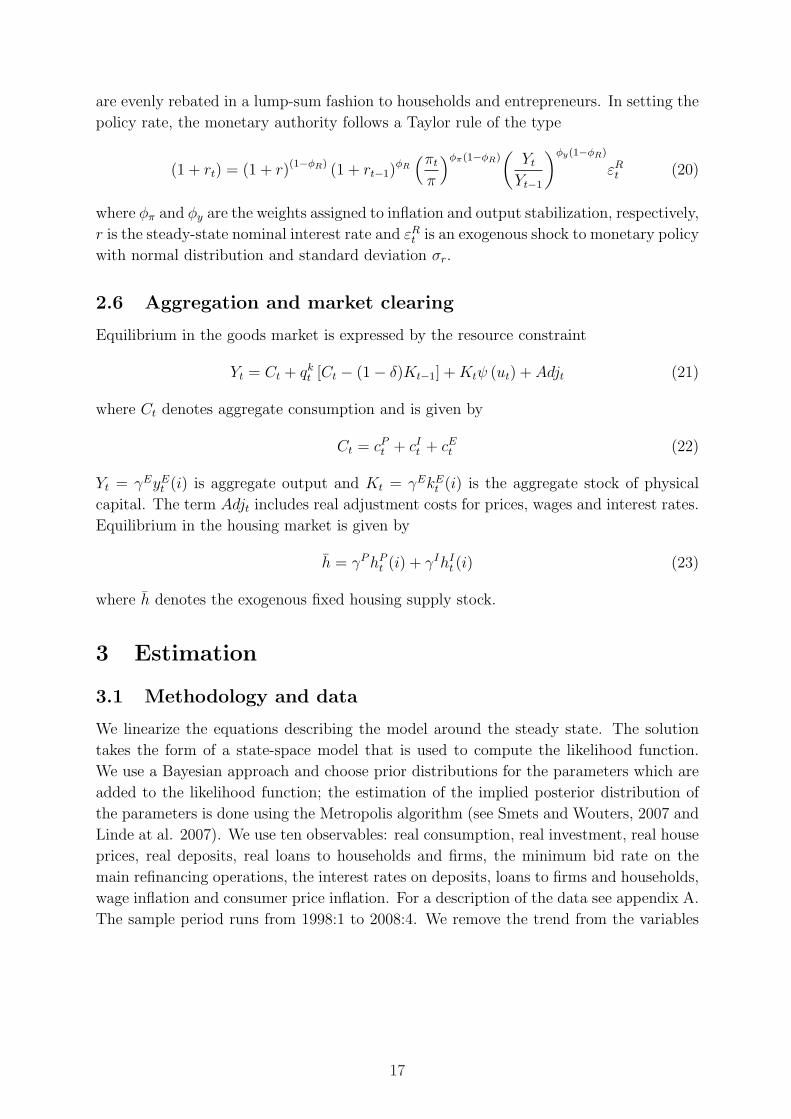
are evenly rebated in a lump-sum fashion to households and entrepreneurs. In setting the

policy rate, the monetary authority follows a Taylor rule of the type

(1 + rt) = (1 + r)(1−φR) (1 + rt−1)φR

(πt

π

)φπ(1−φR)(

Yt

Yt−1

)φy(1−φR)

εRt (20)

where φπ and φy are the weights assigned to inflation and output stabilization, respectively,

r is the steady-state nominal interest rate and εRt is an exogenous shock to monetary policy

with normal distribution and standard deviation σr.

2.6 Aggregation and market clearing

Equilibrium in the goods market is expressed by the resource constraint

Yt = Ct + qkt [Ct − (1− δ)Kt−1] + Ktψ (ut) + Adjt (21)

where Ct denotes aggregate consumption and is given by

Ct = cPt + cI

t + cEt (22)

Yt = γEyEt (i) is aggregate output and Kt = γEkE

t (i) is the aggregate stock of physical

capital. The term Adjt includes real adjustment costs for prices, wages and interest rates.

Equilibrium in the housing market is given by

h = γP hPt (i) + γIhI

t (i) (23)

where h denotes the exogenous fixed housing supply stock.

3 Estimation

3.1 Methodology and data

We linearize the equations describing the model around the steady state. The solution

takes the form of a state-space model that is used to compute the likelihood function.

We use a Bayesian approach and choose prior distributions for the parameters which are

added to the likelihood function; the estimation of the implied posterior distribution of

the parameters is done using the Metropolis algorithm (see Smets and Wouters, 2007 and

Linde at al. 2007). We use ten observables: real consumption, real investment, real house

prices, real deposits, real loans to households and firms, the minimum bid rate on the

main refinancing operations, the interest rates on deposits, loans to firms and households,

wage inflation and consumer price inflation. For a description of the data see appendix A.

The sample period runs from 1998:1 to 2008:4. We remove the trend from the variables

17

using the HP filter. We also estimated the model with linearly detrended and obtained

very similar results in terms of the posterior distribution of the parameters of the model.

We estimate the parameters that affect the dynamics of the model and calibrate those

determining the steady state in order to obtain reasonable values for some key steady-state

values and ratios. Table 1 reports the values of the calibrated parameters.8

3.2 Calibrated parameters and prior distributions

Calibrated parameters We set the patients’ discount factor at 0.9943, in order to

obtain a steady-state interest rate on deposits slightly above 2 per cent on an annual basis,

in line with the average monthly rate on M2 deposits in the euro area between January

1998 and December 2008.9 As for impatient households’ and entrepreneurs’ discount

factors βI and βE, we set them at 0.975, in the range suggested by Iacoviello (2005) and

Iacoviello and Neri (2008). The mean value of the weight of housing in households’ utility

function εhj is set at 0.2, close to the value in Iacoviello and Neri (2008). As for the

loan-to-value (LTV) ratios, we set mI at 0.7 in line with evidence for mortgages in the

main euro area countries (0.7 for Germany, 0.5 for Italy and 0.8 for France and Spain), as

pointed out by Calza et al. (2007). The calibration of mE is somewhat more problematic:

Iacoviello (2005) estimates a value of 0.89, but, in his model, only commercial real estate

can be collateralized; Christensen et al. (2007), estimate a much lower value (0.32), in a

model for Canada where firms can borrow against business capital. Using data over the

period 1999-2008 for the euro area we estimate an average ratio of long-term loans to the

value of shares and other equities for the non financial corporations sector of around 0.41;

using short-term instead of long-term loans we obtain a smaller value of around 0.2. Based

on this evidence, we decide to set mE at 0.25. These LTV ratios imply a steady-state

shares of household and entrepreneur loans equal to 49 and 51 per cent, respectively.

The capital share is set to 0.25 and the depreciation rate to 0.025. In the labor market

we assume a markup of 15 per cent and set εl at 5. In the goods market, a value of 6 for εy

in steady state delivers a markup of 20 percent, a value commonly used in the literature.

For the banking parameters, no corresponding estimates are available in the literature.

Thus, we calibrate them so as to replicate some statistical properties of bank interest

rates and spreads. Equation (16) shows that the steady-state spread between the deposit

8 Estimation is done with Dynare 4.0.9 The rate on M2 deposits was constructed by taking a weighted average of the rates on overnight

deposits, time deposits up to 2 years and saving deposits up to 3 months, with the respective outstandingamounts in each period as weights. Data on interest rates were obtained from the official MIR statisticsby the ECB, starting from January 2003; previous to that date, we used monthly variations of non-harmonized interest rates for the EMU-12, provided by the BIS, to reconstruct back the series. Similarly,for loan rates we used ECB official interest rates on new-business loans to non-financial corporations andon loans for house purchase to households since January 2003, and we reconstructed back the series byusing variations of non-harmonized rates before that date.

18

rate and the interbank rate depends on εdt ; thus, to calibrate εd we calculate the average

monthly spread between banking rates in our sample and the 3-month Euribor, which

corresponds to around 150 basis points on an annual basis, implying that εd = −1.3.

Analogously, we calibrate εbHt and εbE

t by exploiting the steady-state relation between the

marginal cost of loan production and household and firm loan rates. The steady state

ratio of bank capital to total loans (BHt + BE

t ) is set to 0.09, slightly above the capital

requirements imposed by Basel II. The parameter δb is set at the value (0.0982) that

ensures that the ratio of bank capital to total loans is exactly 0.09.

Prior distributions Our priors are listed in Tables 2A and 2B. Overall, they are

either consistent with the previous literature or relatively uninformative. For the persis-

tence, we choose a beta-distribution with a prior mean of 0.8 and standard deviation of

0.1. We set the prior mean of the habit parameters in consumption ah = aP = aI = aE

at 0.5 (with a standard error of 0.1). For the monetary policy specification, we assume

prior means for φR, φπ and φY equal, respectively, to 0.75, 2.0 and 0.1. We set the prior

mean of the parameters measuring the adjustment costs for prices κp and wages κw to,

respectively, 50 and 100 with standard deviations of 50. The priors for the indexation

parameters ιp and ιw are loosely centered around 0.5, as in Smets and Wouters (2007).

As for the mean of the adjustment costs for interest rates, their mean is set to 20 and the

standard deviation to 10. These priors include the values that have been estimated using

a small scale VAR, which included the bank interest rates on deposits, loans to households

and loans to firms, the three-month money market rate and a monthly measure of output,

estimated over the period 1999:1 2008:12. The impact response to an exogenous increase

of 25 basis points in the three-month rate is equal to 3 basis points for the interest rate on

deposits, and to 17 and 15 basis points for the interest rates on loans to households and

to firms, respectively. These responses imply adjustment costs equal to 11 for deposits

(κd), 6 for loans to households (κbH) and 5 for the loans to firms (κbE).

3.3 Posterior estimates

Tables 2A and 2B report the posterior mean, median and 95 probability intervals for the

structural parameters, together with the mean and standard deviation of the prior distri-

butions. Draws from the posterior distribution of the parameters are obtained using the

random walk version of the Metropolis algorithm. We run 10 parallel chains each of length

200,000. The scale factor was set in order to deliver acceptance rates between 20 and 30

percent. Convergence was assessed by means of the multivariate convergence statistics

taken from Brooks and Gelman (1998). Figures 2 and 3 report the prior and posterior

marginal densities of the parameters of the model, excluding the standard deviation of

the innovations of the shocks.

All shocks are quite persistent with the only exception of the price markup shock. As

19

far as monetary policy is concerned our estimation confirm the weak identification of the

response to inflation (see Figure 3) and the relatively large degree of interest rate inertia.

The posterior median of the coefficient measuring the response to output growth is larger

(3) than the prior mean. Concerning nominal rigidities, we find that wage stickiness is

more important than price stickiness. The degree of price indexation is relatively low (the

median is 0.15) and confirms the finding of Benati (2008) who documents a reduction in

indexation in the euro area in the post-1999 sample. Concerning the parameters measuring

the degree of stickiness in bank rates, we find that deposit rates adjustment more rapidly

than the rates on loans to changes in the policy rate. This results is not surprising given

that our measure of deposits include also time and saving deposits. The interest rates on

these instruments, indeed, is typically more responsive to changes in money market rates

than those on overnight deposits. In all the cases the median is smaller than the mean of

the prior distribution.

The median values of the marginal posterior distribution of the parameters We set the

prior mean of the parameters measuring the adjustment costs for prices κp and wages κw

to, respectively, 50 and 100 with standard deviations of 50. The priors for the indexation

parameters ιP and ιW are loosely centered around 0.5, as in Smets and Wouters (2007).

As for the mean of the adjustment costs for interest rates, their mean is set to 20 and the

standard deviation to 10.

4 Properties of the estimated model

In this Section we study the dynamics of the linearized model using impulse responses,

focusing on a contractionary monetary policy shock and on an expansionary technology

innovation. Our aim is to assess whether and how the transmission mechanism of mone-

tary and technology shocks is affected by the presence of financial frictions and financial

intermediation and how different our findings are from those of other papers that share

some of our features, such as Iacoviello (2005), Christiano et al. (2007) or Goodfriend

and McCallum (2007). At the same time we want to analyze the impact of this types of

shocks on the profitability and capital position of financial intermediaries, a task that our

model is suited to accomplish.

4.1 Monetary policy shock

The transmission of a monetary policy shock is first studied by analyzing the impulse

responses to an unanticipated 50 basis points exogenous shock to the policy rate (rt) (see

Figure 4). The benchmark model, described in the previous sections, features a number of

transmission channels for monetary impulses. Besides the traditional interest rate channel,

modified by the presence of agents with an heterogeneous degree of patience, there exist

20

three more channels: a borrowing constraint channel by which an innovation in the policy

rate, by changing the net present value of the collateral, changes how binding agents’

constraints are; moreover, there exist a financial accelerator effect, by which induced

changes in asset price alter the value of the collateral agents can pledge. Finally, the

assumption that interest and principal payments on loans and deposits are in nominal

terms introduces a nominal debt channel, whereby changes in inflation affect the ex-post

distribution of resources across borrowers and lenders. All these last three factors have

been shown to contribute to amplify and propagate the initial impulse of a monetary

tightening (see, e.g., Iacoviello, 2005, or Calza et al., 2007). Adding to their effects, the

presence of a banking sector affects the monetary transmission mechanism by impinging

on each of them. In particular, credit market power, sluggishness in bank rates and the

presence of bank capital might dig wedges between rates set by the policymaker and rates

which are relevant for the decisions of each agent in the economy. The overall effect on

the transmission mechanism of monetary policy could in principle be ambiguous.

In order to highlight how the various channel affect the transmission of monetary policy,

in figure 4 we compare our (benchmark) model (BK in the figure) with a number of other

models, where we progressively shut down a number of features: (i) a model where we

shut down the bank-capital channel, i.e. a model with a simplified balance-sheet for banks,

including only deposits on the liability side (noBK in the figure);10 (ii) a model where

we also remove stickiness in bank-interest rate setting and allow for flexible rates (FR in

the figure); 11 (iii) a model with perfectly competitive banks, i.e. most resembling to the

single interest rate model with financial frictions in Iacoviello (2005) (FF inthe figure);12

(iv) a model where we also remove the financial accelerator and debt-deflation effects, in

order to obtain a model similar to the standard New Keynesian DSGE.13

In the benchmark model, the presence of financial intermediation and capital con-

straints does not qualitatively alter the responses of the main macroeconomic variables,

when compared to standard results in the New Keynesian literature. Therefore, our model

has the advantage to introduce new elements, thus enriching the inter-linkages between

macroeconomic and financial variables, while remaining able to replicate stylized facts in

business cycle theory. In the face of a policy tightening, output and inflation contract

and the policy rate does not rise one-to-one with the exogenous shock, because it endoge-

nously responds to the fall in output and inflation. Loans to both households and firms

fall, reflecting the decline in asset prices, i.e. the price of housing and the value of firms’

10 In order to do so, we force the parameter κKb to be equal to 0 and we rebate banking profits topatient households in a lump-sum fashion.

11 Operationally, we set the costs to change rates κbH , κbE and κd to zero.12 This model is obtained by assuming that the elasticities of substitution for loans and deposits all

equal infinity.13 Here agents are assumed to be still constrained in borrowing but at the steady state value of the

collateral, and loans and deposits (plus interest) are repaid in real terms.

21

capital, and the increase in the real interest rate. Bank loan rates increase less than the

policy rate (on impact, the increase is around one fourth) but they remain above steady

state for longer, reflecting the imperfect pass-through of lending rates; the loan-deposit

interest margin also goes up, as the increase in the deposit rate is even less pronounced.

The response of bank capital is initially positive, reflecting the increase in bank margins

and thus profit, but it subsequently falls as spreads reduce and financial activity remains

subdued.

From a quantitative point of view, however, a number of differences arises from the

the introduction of financial intermediation. In general, our banking sector attenuates

the responses with respect to a model featuring a single interest rate (FF model in the

figure). This is because monopolistic competition in banking introduces a steady-state

wedge between retail bank rates and the policy rates, on the one hand, and also allows for

imperfect pass-through on bank rates (due to adjustment costs) which mutes the response

of retail rates to the increase in the official rate. The introduction of a link between the

capital position of banks and the spread on loans has, instead, virtually no effect on

the dynamics of the real variables; this partly reflects the small value estimated for the

parameter κKb, which - as mentioned before - we use to perform this exercise. To give

an example, our calibration implies that a reduction of the capital-to-asset ratio by half

(from its steady state value of 9%) would increase the spread between loan rates and the

policy rate by only 20 basis points.

Analyzing more in detail the differences between the various models, the presence of the

financial accelerator is clearly evident when comparing the model with financial frictions

(and no banks; FF model) with the model where this channel is shut down (QNK model).

The role of banks begins to appear when we take into account the responses of the FR

and of the noBK models, which add a (simplified) banking sector to the FF framework; in

both these models, there is a wedge between active and passive rates as a consequence of

the market power of banks and pass-through on bank rates is imperfect. The FR model

isolates the attenuating effect coming from imperfect competition in the credit market.

This comes from a steady state effect according to which a given (absolute) monetary

tightening impinges on a loan rate which is already higher, by a measure of the markup,

than the policy rate, therefore determining a smaller percent variation of the former

rate. Sticky bank rates (noBK model) add to this, preventing banks to fully pass on the

policy rate increase to retail rates. From the figure, it is evident that the attenuator effect

resulting from the presence of banks can be sizeable on impact. Finally, when we compare

the noBK and the BK model, we disentangle the effect on real variables of the presence of

banking capital. Bank capital rises substantially following the shock but turns negative

after 10 quarters; overall, the impact of the shock is very persistent, suggesting that the

introduction of this feature can potentially add much to the propagation mechanism.

Movements in bank capital follow the dynamics of bank profits (which in our model

22

correspond to interest margin): these rise on impact, when the increase in rate spreads

more than offsets the fall in intermediated funds, but later become negative (after around

5 quarters), when spreads reduce to zero (and intermediation activity remains subdued).

The increase in equity seems to determine some substitution effect with deposits, whose

relative cost has increased; such substitution prevents movements in equity to have any

significant impact on credit and, thus, on the real economy.

Our findings about the relative strength of the effects coming from the financial fric-

tions and the banking sector are in line with much of the available literature. Christensen

et al. (2007) find that financial frictions boost the response of output after an increase

in policy rates by about a third, mainly on account of a stronger response of both con-

sumption and investment. As for the role of banks, Christiano et al. (2007) find that, in

general, the presence of banks and financial frictions strengthens significantly the prop-

agation mechanism of monetary policy: the output response is both bigger and more

persistent compared to a model that does not feature these channels. Although their

banks, compared to ours, are rather different intermediaries that operate under perfect

competition, they also find that banks play a marginal role in propagating the monetary

impulse while the financial accelerator is more important. An attenuation effect coming

from banks similar to ours has been found in Goodfriend and McCallum (2007) banking

model. In their model, the effect occurs only when the monetary impulse is very persis-

tent, since marginal costs in the banking sector become procyclical in that case (otherwise

the effect is of opposite sign). The attenuation effect in our model is more general, as

bank rate adjustment is sluggish irrespective of the persistence of monetary shocks. A

similar attenuator effect from the presence of a steady-state spread in the banking sector,

due to imperfectly competitive financial intermediation, arises also in Andres and Arce

(2008) and Aslam and Santoro (2008).

4.2 Technology shock

The transmission of a technology shock is studied by looking at the impulse responses

coming from the same set of models illustrated in the previous paragraph. Figure 5 shows

the simulated responses of the main macroeconomic and financial variables following a

shock to aEt equal in size to the estimated standard deviation of TFP.

In the case of a technology shock the presence of financial intermediation substantially

enhances the endogenous propagation mechanism after the shock, with output peaking

higher and 2 to 4 quarters later than in the model with financial frictions and without

banks (FF). This effect reflects mainly the behavior of investment, whose response is

significantly magnified by the presence of financial intermediaries.

In all models, the shock makes production more efficient, bringing inflation down.

Monetary policy accommodates the fall in inflation bringing down also loan rates, and

23

therefore increasing loans, aggregate demand and output. When we introduce a monopo-

listically competitive banking sector (with flexible rates, FR), the reduction in the policy

rate translates into a reduction of credit spreads, which increases the demand for loans.

Both impatient households and entrepreneurs, benefitting from the greater availability

of credit, accumulate housing and physical capital, which allows them to borrow even

more and to enjoy a persistent expansion of consumption. As a result, there the effects of

the shock on both consumption and investment is more persistent: the peak increase in

consumption is reached in the beginning of the third year, i.e. one year later with respect

to the model without banks; the rise in investment is very pronounced and also its peak

is delayed.

When we add to this basic mechanism sticky bank rates (the noBK model) the pic-

ture does not change substantially, although the reduction of spreads is dampened by

the imperfect pass-through, determining a smaller impact reaction of lending and, thus,

of consumption and investment. The introduction of bank capital has a relevant impact

on investment, going mainly through the reduction of the availability of credit to en-

trepreneurs. In addition, the reduction in capital - by affecting the bank capital position

- also affects the loan margin, dampening the reduction described above.

5 Applications

Once the model has been estimated and its propagation mechanism studied, we can use

it to address the two questions raised in the Introduction. First, what role did the shocks

originating in the banking system played in the dynamics of the main variables since the

burst of the financial crisis? Second, what are the effects of a credit crunch originating

from a fall in bank capital?

5.1 The role of financial shocks in the business cycle

In order to quantify the relative importance of each shock in the model we perform an

historical decomposition of the dynamics of the main macro and financial variables of

the euro area. This decomposition was obtained by fixing the parameters of the model

at the posterior mode and then using the Kalman smoother to obtain the values of the

innovations for each shock. The aim of the exercise is twofold: on the one hand, we want

to investigate how our financially-rich model interprets the slowdown in 2008 and thus

learn from the model which shocks were mainly responsible for the current slowdown. On

the other hand, to the extent that the overall story told by the model is consistent with

the common wisdom emerged so far about the origins and causes of the current crises, we

can use this experiment as an indirect misspecification test for our model.

For this exercise we have divided the 13 shocks that appear in the model in three groups.

24

First there is a “macroeconomic” group, which pulls together shocks to the production

technology, to intertemporal preferences, to housing demand, to the investment-specific

technology, and to price and wage markups. Then, the “monetary policy” group isolates

the contribution coming from the non-systematic conduct of the monetary policy. Finally,

the “financial” group consists of shocks originating in the banking system: those are the

shocks to the loan-to-value ratios on loans to firms and households, the shocks to the

markup on the bank interest rates and the shock to the balance sheet.

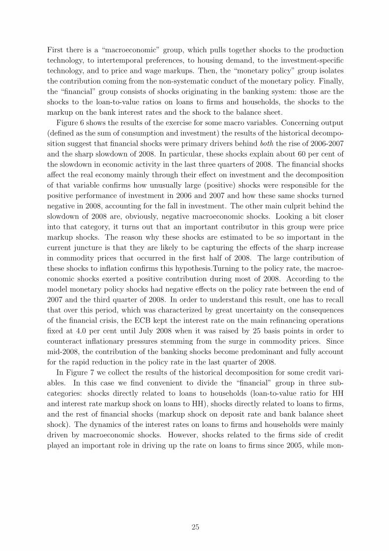
Figure 6 shows the results of the exercise for some macro variables. Concerning output

(defined as the sum of consumption and investment) the results of the historical decompo-

sition suggest that financial shocks were primary drivers behind both the rise of 2006-2007

and the sharp slowdown of 2008. In particular, these shocks explain about 60 per cent of

the slowdown in economic activity in the last three quarters of 2008. The financial shocks

affect the real economy mainly through their effect on investment and the decomposition

of that variable confirms how unusually large (positive) shocks were responsible for the

positive performance of investment in 2006 and 2007 and how these same shocks turned

negative in 2008, accounting for the fall in investment. The other main culprit behind the

slowdown of 2008 are, obviously, negative macroeconomic shocks. Looking a bit closer

into that category, it turns out that an important contributor in this group were price

markup shocks. The reason why these shocks are estimated to be so important in the

current juncture is that they are likely to be capturing the effects of the sharp increase

in commodity prices that occurred in the first half of 2008. The large contribution of

these shocks to inflation confirms this hypothesis.Turning to the policy rate, the macroe-

conomic shocks exerted a positive contribution during most of 2008. According to the

model monetary policy shocks had negative effects on the policy rate between the end of

2007 and the third quarter of 2008. In order to understand this result, one has to recall

that over this period, which was characterized by great uncertainty on the consequences

of the financial crisis, the ECB kept the interest rate on the main refinancing operations

fixed at 4.0 per cent until July 2008 when it was raised by 25 basis points in order to

counteract inflationary pressures stemming from the surge in commodity prices. Since

mid-2008, the contribution of the banking shocks become predominant and fully account

for the rapid reduction in the policy rate in the last quarter of 2008.

In Figure 7 we collect the results of the historical decomposition for some credit vari-

ables. In this case we find convenient to divide the “financial” group in three sub-

categories: shocks directly related to loans to households (loan-to-value ratio for HH

and interest rate markup shock on loans to HH), shocks directly related to loans to firms,

and the rest of financial shocks (markup shock on deposit rate and bank balance sheet

shock). The dynamics of the interest rates on loans to firms and households were mainly

driven by macroeconomic shocks. However, shocks related to the firms side of credit

played an important role in driving up the rate on loans to firms since 2005, while mon-

25

etary policy shocks were relatively important drivers between 2006 and 2007, when the

ECB raised the policy rate from the very low levels reached in June 2003. Concerning

loans to households, a main driver of its dynamics turned out to be the housing shock

(within the macro group), since it explains most of the strong rise in 2006 and 2007 and

of the subsequent decline in 2008. This is not surprising given the role of housing as

collateral for the households in obtaining credit. Beside the housing shock, a important

role in the recent fall is played by the high price markup shocks (within the macro group)

estimated in 2008, which, as we said earlier, are likely to be capturing the sharp increase

in commodity prices that occurred in the first half of 2008. Loans to firms are driven

almost exclusively by shocks related directly to the firms side of credit, with the notable

exception of 2008 when a sizable negative contribution comes from the macroeconomic

shocks (in particular, again, the price markups).

To sum up, the exercise taught us that the banking shocks introduced in our model have

played an important role in shaping the dynamics of the euro area in the last business

cycle and, more importantly, according to the model they did so in a way that nicely

squares with our prior knowledge and expert judgement of macroeconomists about what

has happened.

5.2 The effects of a tightening of credit conditions

Starting in the summer of 2007, financial markets in a number of advanced economies fell

under considerable strain. The initial deterioration in the US sub-prime mortgage market

quickly spread across other financial markets, affecting the valuation of a number of assets.

Banks, in particular, suffered losses from significant write-offs on complex instruments

and reported increasing funding difficulties, in connection with the persisting tensions in

the interbank market and with the substantial hampering of securitization activity. A

number of them were forced to recapitalize and improve their balance sheets. In addition,

intermediaries reported that concerns over their liquidity and capital position induced

them to tighten credit standards for the approval of loans to the private sector. In the euro

area, since the October 2007 round, banks participating to the Eurosystem’s quarterly

Bank Lending Survey reported to have strongly increased the margins charged on average

and riskier loans and to have implemented a restriction on collateral requirements both

for households and firms; in each 2008 Survey release, 30% of respondent banks reported

to have reduced the loan-to-value ratio for house purchase mortgages in the previous three

months. Against this background, policymakers have been particularly concerned with

the impact that a restriction in the availability and cost of credit might have on the real

economy. The potential consequences on economic activity of the financial turmoil have

been given considerable attention when evaluating the appropriateness of the monetary

policy stance.

In light of the importance of understanding the consequences of a tightening of credit

26

standards by banks, in this section we try to answer the following question: What would

happen if bank capital were to suffer a strong negative shock? Would it trigger a contrac-

tion in loan supply, an increase in bank rates and a contraction in economic activity?

Our model is well-suited to analyze the effects of a tightening in credit conditions on the

real activity and to give indications (at least qualitatively) on the appropriate response

of a central bank following a Taylor-type monetary policy rule. The experiment we carry

out involves implementing an unexpected and persistent contraction in bank capital Kb.

We do not attempt to construct a quantitatively realistic scenario; this would be indeed

very difficult, given the conflicting indications coming from hard and survey evidence on

the tightening of credit standards, in particular in the euro area, and the uncertainty on

the effects that have already occurred and on those that might still be in the pipeline.

We calibrate the shock in a way that it determines a fall of bank capital by 5 percent

on impact. The persistence of the shock is set to 0.95 in order to obtain a persistent

fall of the capital/asset ratio below its steady state value (9 percent). In the exercise we

assess the role of the adjustment costs on the capital/asset ratio by computing the impulse

responses under different calibration of the parameters κKb. We consider as benchmark

a value of 10, the prior mean of the parameters, and then a higher one, corresponding to

50, and a lower one equal to 2. Figure 8 shows the effect of this credit crunch experiment.

By construction, the credit tightening brings about a fall in bank capital. In order to

compensate for the loss in equity, banks increase the rate on deposits to attract them and

increase their liabilities. At the same time, they increase the rates on loans to increase

profits. At this point, the larger is the cost for adjusting the capital ratio, the larger is the

increase in banks’ interest rates. Higher rates reduce the demand for loans by households

and firms which are forced to cut back on consumption and investment expenditure. The

effect is larger on investment; the size of the response of consumption depends largely

on the persistence of the shock to bank capital (see Figure 8). When the persistence of

the shock is reduced to 0.5, consumption marginally increases while investment still falls

substantially. Output contracts only when the adjustment costs on the capital ratio is

sufficiently large. In this scenario, interest rates on loans and deposits still increase and

loan demand falls; profits increase and compensate the fall in equity. The capital ratio

converges faster to its steady state.

Looking at individual agents, the rate shock unfavorably hits impatient households,

through the increase in the real interest rate they face on loans, who are forced to sell their

housing in order to support consumption. House prices fall and patient households start

investing in housing by reducing consumption. Entrepreneurs reduce the accumulation

of capital and consumption. Aggregate demand falls considerably and output contracts

significantly.

27

6 Concluding remarks

The paper has presented a model in which both entrepreneurs and impatients households

face borrowing constraints and loans are supplied by imperfectly competitive banks that

collect deposits from patient households. Deposits and bank capital are used to produce

loans that are granted to households and firms. Bank interest rates on these distinct loans

and on deposits adjust slowly to changes in the policy rate. The model is estimated using

Bayesian techniques and data for the euro area over the period 1999-2008.

We find that in the face of demand shocks, like a monetary policy shock, the presence

of financial intermediaries diminishes the business cycle acceleration effects deriving from

a change of the real net present value of agents’ collateral. The presence of bank capital

does not alter the effects of monetary policy shocks on the main macroeconomic variables.

On the contrary, banks intermediation increases the propagation of supply shock like

technological improvements.

The model is then used to quantify the contribution of shocks originating within the

banking sector to the slowdown in economic activity during 2008 and to study the conse-

quences of tightening of credit conditions induced by a reduction in bank capital. Shocks

in the banking sector explain the largest fraction of the fall output in 2008 while macroeco-

nomic shocks played a smaller role. The effects of a credit supply shock can be substantial

particularly on investment. A fall in bank capital forces bank to raise interest rates re-

sulting in lower demand for loans by households and firms who are forced to cut on

consumption and expenditure.

28

References

[1] Andres, J. and O. Arce (2008), Banking Competition, Housing Prices and Macroe-

conomic Stability, mimeo, Bank of Spain.

[2] Aslam, A. and E. Santoro (2008), Bank Lending, Housing and Spreads, University

of Copenhagen, Department of Economics Discussion Papers, No. 08-27.

[3] Benes, J. and K. Lees (2007), Monopolistic Banks and Fixed Rate Contracts: Impli-

cations for Open Economy Inflation Targeting, mimeo, Reserve Bank of New Zealand.

[4] Bernanke, B.S. and M. Gertler (1995), “Inside the Black Box: The Credit Channel

of Monetary Policy Transmission.” Journal of Economic Perspectives, Vol. 9(4), pp.

27-48.

[5] Bernanke, B.S., M. Gertler and S. Gilchrist (1999), “The Financial Accelerator in

a Quantitative Business Cycle Framework”, in J.B. Taylor and M. Woodford, eds.,

Handbook of Macroeconomics, North-Holland, pp. 1341-1393.

[6] Calza, A., T. Monacelli and L. Stracca (2007), “Mortgage Markets, Collateral Con-

straints, and Monetary Policy: Do Institutional Factors Matter?”, Center for Finan-

cial Studies, Working paper No. 10.

[7] Carlstrom, T.C. and T.S. Fuerst (1997), “Agency costs, net worth, and business fluc-

tuations: a computable general equilibrium analysis”, American Economic Review,

Vol. 87(5), pp. 893-910.

[8] Carlstrom, T.C. and Fuerst T.S. (2006), “Co-Movement in Sticky Price Models with

Durable Goods”, Federal Reserve Bank of Cleveland Working Paper 06-14.

[9] Christensen, I., P. Corrigan, C. Mendicino and S. Nishiyama (2007), “An Estimated

Open-Economy General Equilibrium Model with Housing Investment and Financial

Frictions”, mimeo, Bank of Canada.

[10] Christiano, L., M. Eichenbaum and C. Evans (2005), “Nominal Rigidities and the

Dynamic Effects of a Shock to Monetary Policy” Journal of Political Economy, Vol.

113(1), pp. 1-46.

[11] Christiano, L., R. Motto and M. Rostagno (2007), “Financial Factors in Business

Cycle” mimeo, European Central Bank and Northwestern University.

[12] Curdia, V. and M. Woodford (2008), “Credit Frictions and Optimal Monetary Policy”

mimeo, October.

29

[13] de Bondt, G. (2005), “Interest rate pass-through: Empirical results for the Euro

Area”, German Economic Review, Vol. 6(1), pp. 37-78.

[14] Goodfriend, M. and B.T. McCallum (2007). “Banking and interest rates in monetary

policy analysis: A quantitative exploration” Journal of Monetary Economics, vol.

54(5), pp. 1480-1507.

[15] Iacoviello, M. (2005), “House Prices, Borrowing Constraints and Monetary Policy in

the Business Cycle” American Economic Review, Vol. 95(3), pp. 739-764.

[16] Iacoviello, M. and Neri S. (2008), “Housing market spillovers: evidence from an

estimated DSGE model”, Banca d’Italia Discussion papers, no. 659.

[17] Kiyotaki, N. and J. Moore (1997) “Credit Cycles”, Journal of Political Economy,

Vol. 105(2), pp. 211-248.

[18] Kok Sorensen, C. and T. Werner (2006), “Bank interest rate pass-through in the euro

area: a cross country comparison”, Working paper series, no. 580, European Central

Bank.

[19] Schmitt-Grohe, S. and M. Uribe (2005), “Optimal Fiscal and Monetary Policy in a

Medium-Scale Macroeconomic Model”, in Gertler, M. and K. Rogoff, eds., NBER

Macroeconomics Annual 2005, MIT Press: Cambridge MA, 2006, pp. 383-425.

[20] Smets, F. and R. Wouters (2003), “An Estimated Dynamic Stochastic General Equi-

librium Model Of The Euro Area”, Journal Of The European Economic Association,

Vol. 1(5), pp. 1123-1175.

30

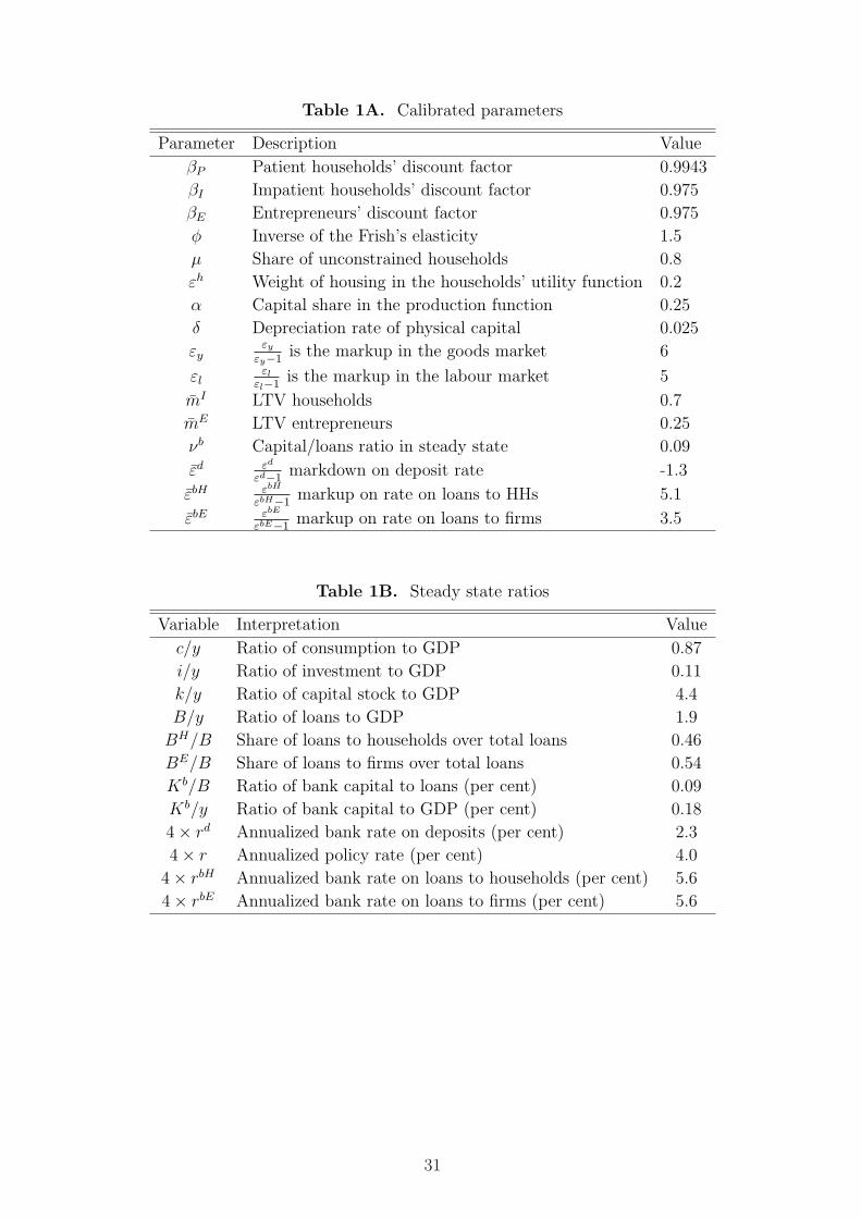
Table 1A. Calibrated parameters

Parameter Description Value

βP Patient households’ discount factor 0.9943

βI Impatient households’ discount factor 0.975

βE Entrepreneurs’ discount factor 0.975

φ Inverse of the Frish’s elasticity 1.5

µ Share of unconstrained households 0.8

εh Weight of housing in the households’ utility function 0.2

α Capital share in the production function 0.25

δ Depreciation rate of physical capital 0.025

εyεy

εy−1is the markup in the goods market 6

εlεl

εl−1is the markup in the labour market 5

mI LTV households 0.7

mE LTV entrepreneurs 0.25

νb Capital/loans ratio in steady state 0.09

εd εd

εd−1markdown on deposit rate -1.3

εbH εbH

εbH−1markup on rate on loans to HHs 5.1

εbE εbE

εbE−1markup on rate on loans to firms 3.5

Table 1B. Steady state ratios

Variable Interpretation Value

c/y Ratio of consumption to GDP 0.87

i/y Ratio of investment to GDP 0.11

k/y Ratio of capital stock to GDP 4.4

B/y Ratio of loans to GDP 1.9

BH/B Share of loans to households over total loans 0.46

BE/B Share of loans to firms over total loans 0.54

Kb/B Ratio of bank capital to loans (per cent) 0.09

Kb/y Ratio of bank capital to GDP (per cent) 0.18

4× rd Annualized bank rate on deposits (per cent) 2.3

4× r Annualized policy rate (per cent) 4.0

4× rbH Annualized bank rate on loans to households (per cent) 5.6

4× rbE Annualized bank rate on loans to firms (per cent) 5.6

31

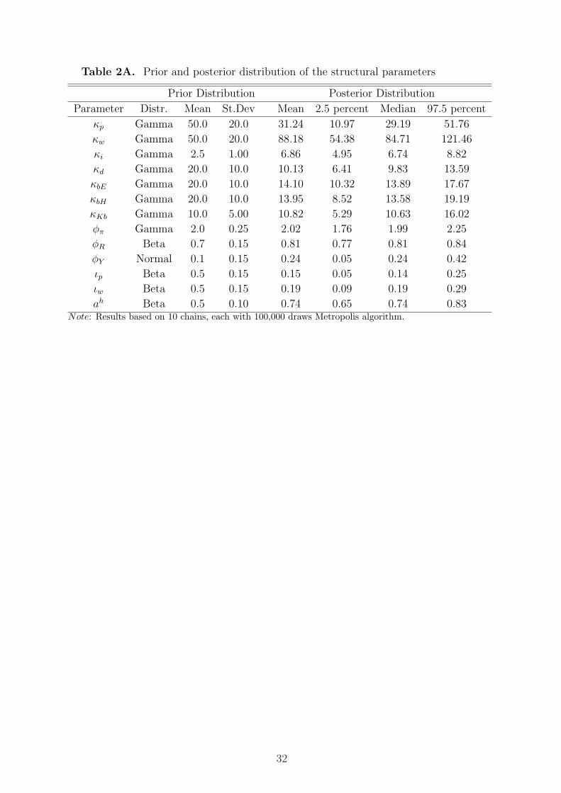
Table 2A. Prior and posterior distribution of the structural parameters

Prior Distribution Posterior Distribution

Parameter Distr. Mean St.Dev Mean 2.5 percent Median 97.5 percent

κp Gamma 50.0 20.0 31.24 10.97 29.19 51.76

κw Gamma 50.0 20.0 88.18 54.38 84.71 121.46

κi Gamma 2.5 1.00 6.86 4.95 6.74 8.82

κd Gamma 20.0 10.0 10.13 6.41 9.83 13.59

κbE Gamma 20.0 10.0 14.10 10.32 13.89 17.67

κbH Gamma 20.0 10.0 13.95 8.52 13.58 19.19

κKb Gamma 10.0 5.00 10.82 5.29 10.63 16.02

φπ Gamma 2.0 0.25 2.02 1.76 1.99 2.25

φR Beta 0.7 0.15 0.81 0.77 0.81 0.84

φY Normal 0.1 0.15 0.24 0.05 0.24 0.42

ιp Beta 0.5 0.15 0.15 0.05 0.14 0.25

ιw Beta 0.5 0.15 0.19 0.09 0.19 0.29

ah Beta 0.5 0.10 0.74 0.65 0.74 0.83Note: Results based on 10 chains, each with 100,000 draws Metropolis algorithm.

32

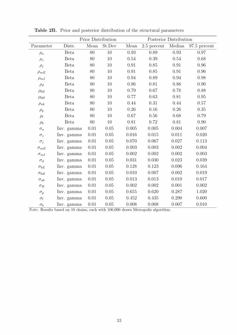
Table 2B. Prior and posterior distribution of the structural parameters

Prior Distribution Posterior Distribution

Parameter Distr. Mean St.Dev Mean 2.5 percent Median 97.5 percent

ρa Beta 80 10 0.93 0.89 0.93 0.97

ρz Beta 80 10 0.54 0.39 0.54 0.68

ρj Beta 80 10 0.91 0.85 0.91 0.96

ρmE Beta 80 10 0.91 0.85 0.91 0.96

ρmI Beta 80 10 0.94 0.89 0.94 0.98

ρd Beta 80 10 0.86 0.81 0.86 0.90

ρbE Beta 80 10 0.79 0.67 0.78 0.88

ρbH Beta 80 10 0.77 0.63 0.81 0.95

ρak Beta 80 10 0.44 0.31 0.44 0.57

ρp Beta 80 10 0.26 0.16 0.26 0.35

ρl Beta 80 10 0.67 0.56 0.68 0.79

ρb Beta 80 10 0.81 0.72 0.81 0.90

σa Inv. gamma 0.01 0.05 0.005 0.005 0.004 0.007

σz Inv. gamma 0.01 0.05 0.016 0.015 0.011 0.020

σj Inv. gamma 0.01 0.05 0.070 0.067 0.027 0.113

σmE Inv. gamma 0.01 0.05 0.003 0.003 0.002 0.004

σmI Inv. gamma 0.01 0.05 0.002 0.002 0.002 0.003

σd Inv. gamma 0.01 0.05 0.031 0.030 0.023 0.039

σbE Inv. gamma 0.01 0.05 0.128 0.123 0.096 0.164

σbH Inv. gamma 0.01 0.05 0.010 0.007 0.002 0.019

σak Inv. gamma 0.01 0.05 0.013 0.013 0.010 0.017

σR Inv. gamma 0.01 0.05 0.002 0.002 0.001 0.002

σp Inv. gamma 0.01 0.05 0.655 0.620 0.287 1.020

σl Inv. gamma 0.01 0.05 0.452 0.435 0.290 0.600

σb Inv. gamma 0.01 0.05 0.008 0.008 0.007 0.010Note: Results based on 10 chains, each with 100,000 draws Metropolis algorithm.

33

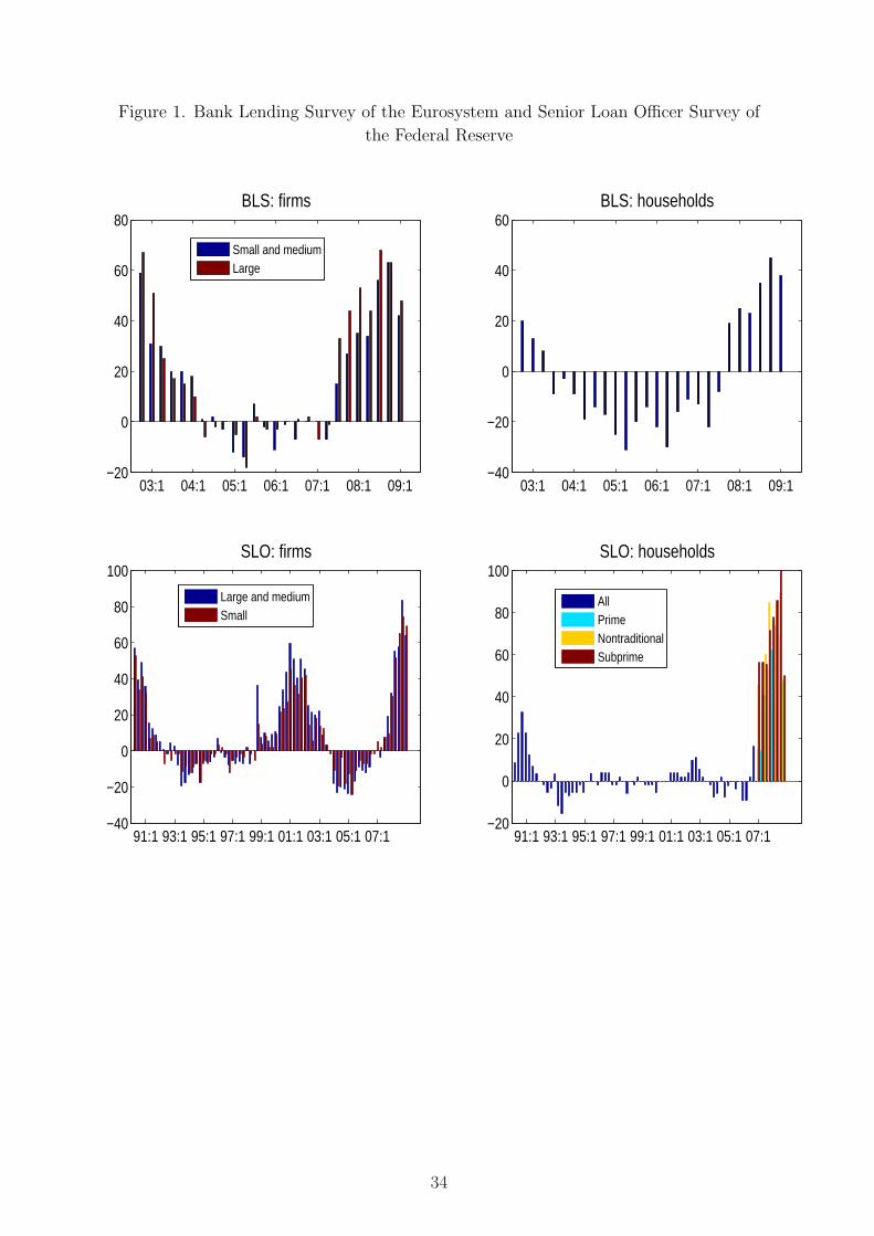
Figure 1. Bank Lending Survey of the Eurosystem and Senior Loan Officer Survey of

the Federal Reserve

03:1 04:1 05:1 06:1 07:1 08:1 09:1−20

0

20

40

60

80BLS: firms

Small and mediumLarge

03:1 04:1 05:1 06:1 07:1 08:1 09:1−40

−20

0

20

40

60BLS: households

91:1 93:1 95:1 97:1 99:1 01:1 03:1 05:1 07:1−40

−20

0

20

40

60

80

100SLO: firms

Large and mediumSmall

91:1 93:1 95:1 97:1 99:1 01:1 03:1 05:1 07:1−20

0

20

40

60

80

100SLO: households

AllPrimeNontraditionalSubprime

34

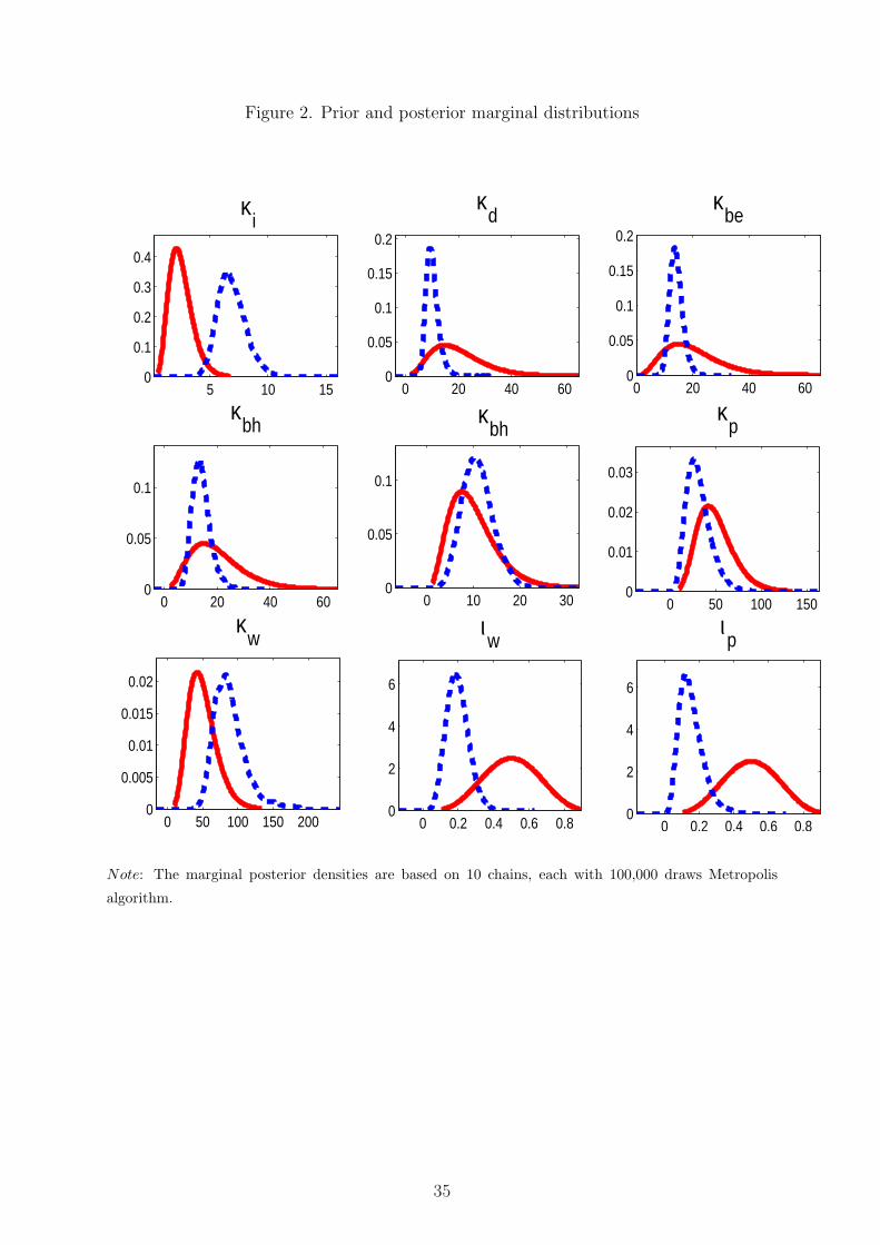
Figure 2. Prior and posterior marginal distributions

0 50 100 150 2000

0.005

0.01

0.015

0.02

κw

0 50 100 1500

0.01

0.02

0.03

κp

0 20 40 600

0.05

0.1

0.15

0.2

κd

0 20 40 600

0.05

0.1

0.15

0.2

κbe

0 20 40 600

0.05

0.1

κbh

0 10 20 300

0.05

0.1

κbh

5 10 150

0.1

0.2

0.3

0.4

κi

0 0.2 0.4 0.6 0.80

2

4

6

ιp

0 0.2 0.4 0.6 0.80

2

4

6

ιw

Note: The marginal posterior densities are based on 10 chains, each with 100,000 draws Metropolis

algorithm.

35

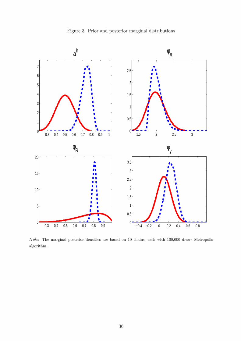
Figure 3. Prior and posterior marginal distributions

0.3 0.4 0.5 0.6 0.7 0.8 0.9 10

1

2

3

4

5

6

7

ah

1.5 2 2.5 30

0.5

1

1.5

2

2.5

φπ

−0.4 −0.2 0 0.2 0.4 0.6 0.80

0.5

1

1.5

2

2.5

3

3.5

φy

0.3 0.4 0.5 0.6 0.7 0.8 0.90

5

10

15

20

φR

Note: The marginal posterior densities are based on 10 chains, each with 100,000 draws Metropolis

algorithm.

36

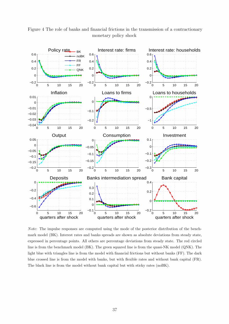
Figure 4 The role of banks and financial frictions in the transmission of a contractionary

monetary policy shock

0 5 10 15 20−0.2

0

0.2

0.4

0.6Policy rate

0 5 10 15 20−0.2

0

0.2

0.4

0.6Interest rate: firms

0 5 10 15 20−0.2

0

0.2

0.4

0.6Interest rate: households

0 5 10 15 20−0.04

−0.03

−0.02

−0.01

0

0.01Inflation

0 5 10 15 20

−0.2

−0.1

0

Loans to firms

0 5 10 15 20

−1

−0.5

0Loans to households

0 5 10 15 20−0.2

−0.15

−0.1

−0.05

0

0.05Output

0 5 10 15 20−0.2

−0.15

−0.1

−0.05

0

Consumption

0 5 10 15 20−0.3

−0.2

−0.1

0

0.1Investment

0 5 10 15 20

−0.6

−0.4

−0.2

0Deposits

quarters after shock0 5 10 15 20

−0.1

0

0.1

0.2

0.3

Banks intermediation spread

quarters after shock0 5 10 15 20

−0.2

0

0.2

0.4Bank capital

quarters after shock

BK

noBK

FR

FF

QNK

Note: The impulse responses are computed using the mode of the posterior distribution of the bench-

mark model (BK). Interest rates and banks spreads are shown as absolute deviations from steady state,

expressed in percentage points. All others are percentage deviations from steady state. The red circled

line is from the benchmark model (BK). The green squared line is from the quasi-NK model (QNK). The

light blue with triangles line is from the model with financial frictions but without banks (FF). The dark

blue crossed line is from the model with banks, but with flexible rates and without bank capital (FR).

The black line is from the model without bank capital but with sticky rates (noBK).

37

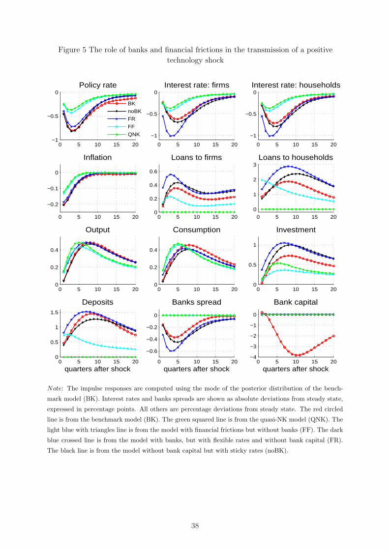
Figure 5 The role of banks and financial frictions in the transmission of a positive

technology shock

0 5 10 15 20−1

−0.5

0Policy rate

0 5 10 15 20

−1

−0.5

0Interest rate: firms

0 5 10 15 20

−1

−0.5

0Interest rate: households

0 5 10 15 20

−0.2

−0.1

0

Inflation

0 5 10 15 200

0.2

0.4

0.6

Loans to firms

0 5 10 15 200

1

2

3Loans to households

0 5 10 15 200

0.2

0.4

Output

0 5 10 15 200

0.2

0.4

Consumption

0 5 10 15 200

0.5

1

Investment

0 5 10 15 200

0.5

1

1.5

Deposits

quarters after shock0 5 10 15 20

−0.6

−0.4

−0.2

0

Banks spread

quarters after shock0 5 10 15 20

−4

−3

−2

−1

0

Bank capital

quarters after shock

BK

noBK

FR

FF

QNK

Note: The impulse responses are computed using the mode of the posterior distribution of the bench-

mark model (BK). Interest rates and banks spreads are shown as absolute deviations from steady state,

expressed in percentage points. All others are percentage deviations from steady state. The red circled

line is from the benchmark model (BK). The green squared line is from the quasi-NK model (QNK). The

light blue with triangles line is from the model with financial frictions but without banks (FF). The dark

blue crossed line is from the model with banks, but with flexible rates and without bank capital (FR).

The black line is from the model without bank capital but with sticky rates (noBK).

38

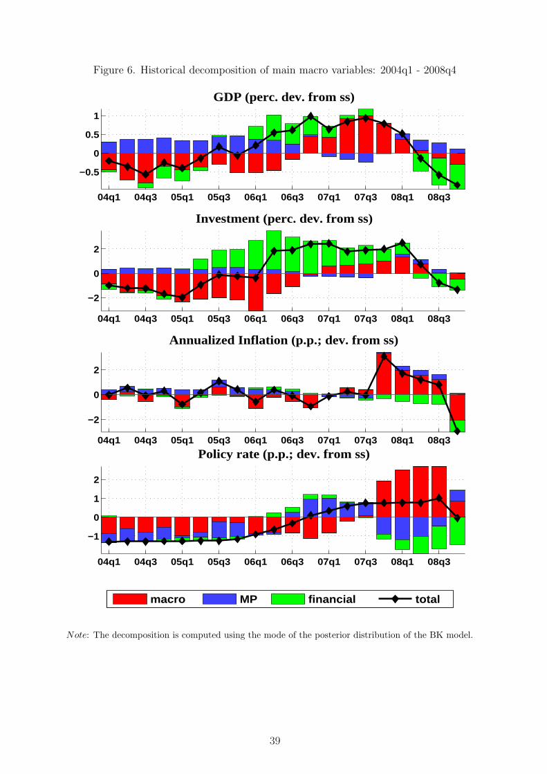
Figure 6. Historical decomposition of main macro variables: 2004q1 - 2008q4

04q1 04q3 05q1 05q3 06q1 06q3 07q1 07q3 08q1 08q3

−0.5

0

0.5

1

GDP (perc. dev. from ss)

04q1 04q3 05q1 05q3 06q1 06q3 07q1 07q3 08q1 08q3

−2

0

2

Investment (perc. dev. from ss)

04q1 04q3 05q1 05q3 06q1 06q3 07q1 07q3 08q1 08q3

−2

0

2

Annualized Inflation (p.p.; dev. from ss)

04q1 04q3 05q1 05q3 06q1 06q3 07q1 07q3 08q1 08q3

−1

0

1

2

Policy rate (p.p.; dev. from ss)

macro MP financial total

Note: The decomposition is computed using the mode of the posterior distribution of the BK model.

39

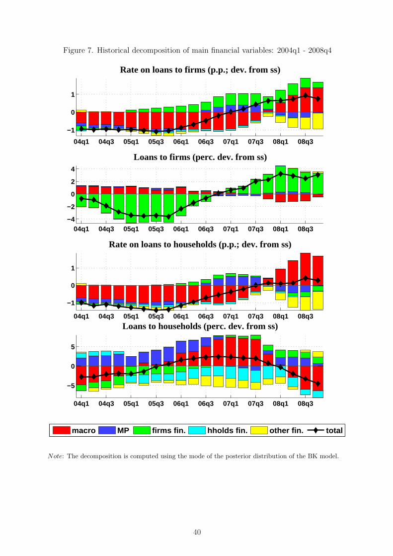
Figure 7. Historical decomposition of main financial variables: 2004q1 - 2008q4

04q1 04q3 05q1 05q3 06q1 06q3 07q1 07q3 08q1 08q3

−1

0

1

Rate on loans to firms (p.p.; dev. from ss)

04q1 04q3 05q1 05q3 06q1 06q3 07q1 07q3 08q1 08q3−4

−2

0

2

4

Loans to firms (perc. dev. from ss)

04q1 04q3 05q1 05q3 06q1 06q3 07q1 07q3 08q1 08q3

−1

0

1

Rate on loans to households (p.p.; dev. from ss)

04q1 04q3 05q1 05q3 06q1 06q3 07q1 07q3 08q1 08q3

−5

0

5

Loans to households (perc. dev. from ss)

macro MP firms fin. hholds fin. other fin. total

Note: The decomposition is computed using the mode of the posterior distribution of the BK model.

40

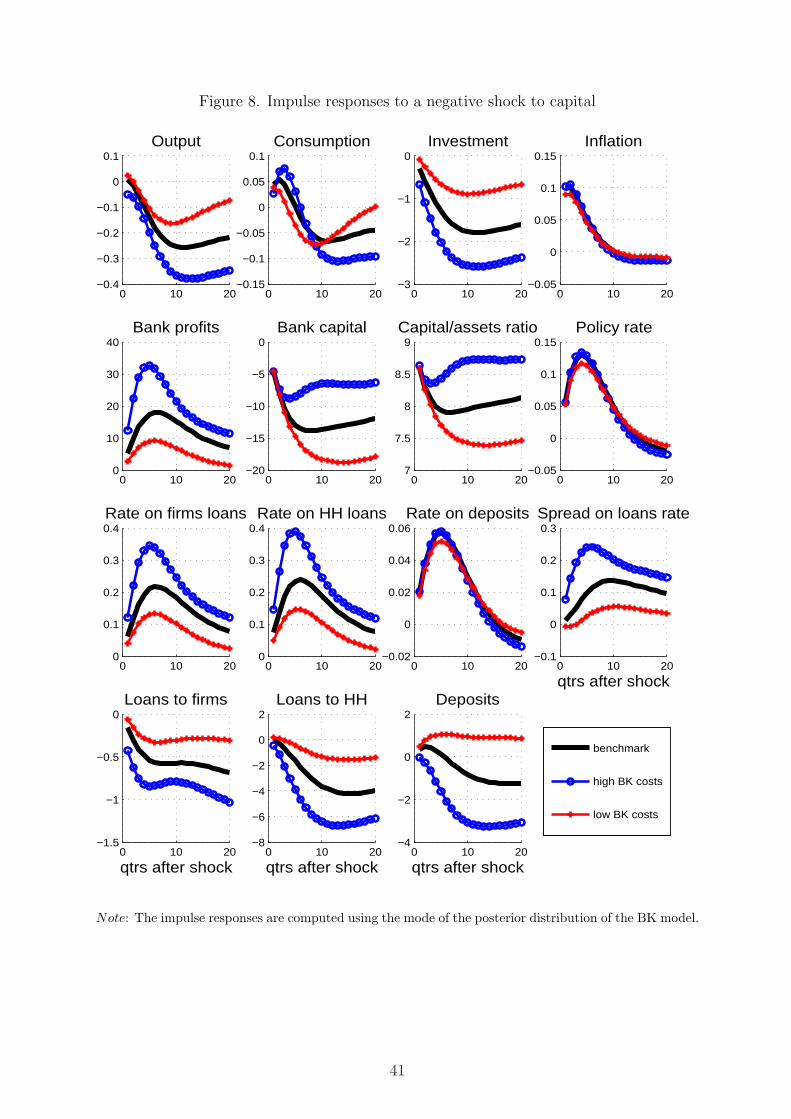
Figure 8. Impulse responses to a negative shock to capital

0 10 20−0.4

−0.3

−0.2

−0.1

0

0.1Output

0 10 20−0.15

−0.1

−0.05

0

0.05

0.1Consumption

0 10 20−3

−2

−1

0Investment

0 10 20−0.05

0

0.05

0.1

0.15Inflation

0 10 200

10

20

30

40Bank profits

0 10 20−20

−15

−10

−5

0Bank capital

0 10 207

7.5

8

8.5

9Capital/assets ratio

0 10 20−0.05

0

0.05

0.1

0.15Policy rate

0 10 200

0.1

0.2

0.3

0.4Rate on firms loans

0 10 200

0.1

0.2

0.3

0.4Rate on HH loans

0 10 20−0.02

0

0.02

0.04

0.06Rate on deposits

0 10 20−0.1

0

0.1

0.2

0.3Spread on loans rate

qtrs after shock

0 10 20−1.5

−1

−0.5

0Loans to firms

qtrs after shock0 10 20

−8

−6

−4

−2

0

2Loans to HH

qtrs after shock0 10 20

−4

−2

0

2Deposits

qtrs after shock

benchmark

high BK costs

low BK costs

Note: The impulse responses are computed using the mode of the posterior distribution of the BK model.

41

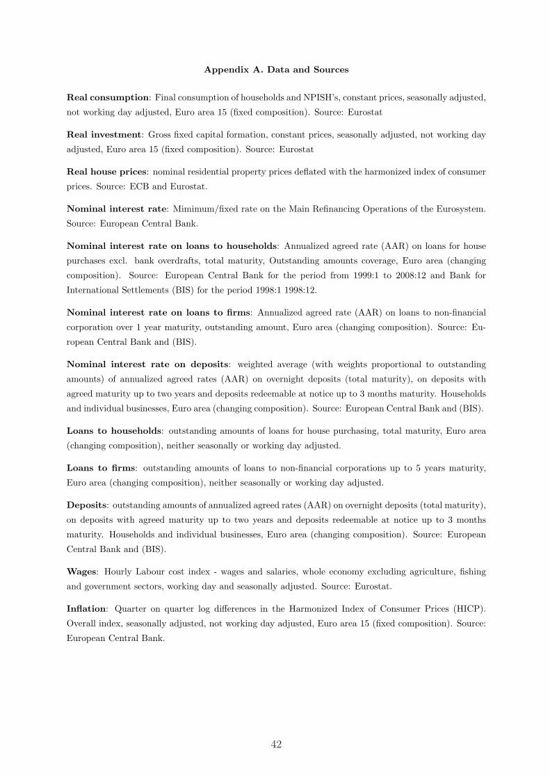
Appendix A. Data and Sources

Real consumption: Final consumption of households and NPISH’s, constant prices, seasonally adjusted,

not working day adjusted, Euro area 15 (fixed composition). Source: Eurostat

Real investment: Gross fixed capital formation, constant prices, seasonally adjusted, not working day

adjusted, Euro area 15 (fixed composition). Source: Eurostat

Real house prices: nominal residential property prices deflated with the harmonized index of consumer

prices. Source: ECB and Eurostat.

Nominal interest rate: Mimimum/fixed rate on the Main Refinancing Operations of the Eurosystem.

Source: European Central Bank.

Nominal interest rate on loans to households: Annualized agreed rate (AAR) on loans for house

purchases excl. bank overdrafts, total maturity, Outstanding amounts coverage, Euro area (changing

composition). Source: European Central Bank for the period from 1999:1 to 2008:12 and Bank for

International Settlements (BIS) for the period 1998:1 1998:12.

Nominal interest rate on loans to firms: Annualized agreed rate (AAR) on loans to non-financial

corporation over 1 year maturity, outstanding amount, Euro area (changing composition). Source: Eu-

ropean Central Bank and (BIS).

Nominal interest rate on deposits: weighted average (with weights proportional to outstanding

amounts) of annualized agreed rates (AAR) on overnight deposits (total maturity), on deposits with

agreed maturity up to two years and deposits redeemable at notice up to 3 months maturity. Households

and individual businesses, Euro area (changing composition). Source: European Central Bank and (BIS).

Loans to households: outstanding amounts of loans for house purchasing, total maturity, Euro area

(changing composition), neither seasonally or working day adjusted.

Loans to firms: outstanding amounts of loans to non-financial corporations up to 5 years maturity,

Euro area (changing composition), neither seasonally or working day adjusted.

Deposits: outstanding amounts of annualized agreed rates (AAR) on overnight deposits (total maturity),

on deposits with agreed maturity up to two years and deposits redeemable at notice up to 3 months

maturity. Households and individual businesses, Euro area (changing composition). Source: European

Central Bank and (BIS).

Wages: Hourly Labour cost index - wages and salaries, whole economy excluding agriculture, fishing

and government sectors, working day and seasonally adjusted. Source: Eurostat.

Inflation: Quarter on quarter log differences in the Harmonized Index of Consumer Prices (HICP).

Overall index, seasonally adjusted, not working day adjusted, Euro area 15 (fixed composition). Source:

European Central Bank.

42