WORKING PAPER NO. 15-41 FISCAL STIMULUS IN ECONOMIC UNIONS:

WHAT ROLE FOR STATES?

Gerald Carlino Federal Reserve Bank of Philadelphia

Robert P. Inman*

The Wharton School of the University of Pennsylvania

November 2015

1

FISCAL STIMULUS IN ECONOMIC UNIONS: WHAT ROLE FOR STATES?

Gerald Carlino Federal Reserve Bank of Philadelphia

Robert P. Inman*

The Wharton School of the University of Pennsylvania

November 2015

Abstract: The Great Recession and the subsequent passage of the American Recovery and Reinvestment Act returned fiscal policy, and particularly the importance of state and local governments, to the center stage of macroeconomic policymaking. This paper addresses three questions for the design of intergovernmental macroeconomic fiscal policies. First, are such policies necessary? An analysis of U.S. state fiscal policies show state deficits (in particular from tax cuts) can stimulate state economies in the short run but that there are significant job spillovers to neighboring states. Central government fiscal policies can best internalize these spillovers. Second, what central government fiscal policies are most effective for stimulating income and job growth? A structural vector autoregression analysis for the U.S. aggregate economy from 1960 to 2010 shows that federal tax cuts and transfers to households and firms and intergovernmental transfers to states for lower income assistance are both effective, with one- and two-year multipliers greater than 2.0. Third, how are states, as politically independent agents, motivated to provide increased transfers to lower income households? The answer is matching (price subsidy) assistance for such spending. The intergovernmental aid is spent immediately by the states and supports assistance to those most likely to spend new transfers.

Keywords: fiscal federalism, intergovernmental aid, aggregate stabilization policy, multiplier analysis JEL Codes: E6, H3, H7, R5 ___________________________________________ *Contact: Carlino: Federal Reserve Bank of Philadelphia, jerry.carlino@phil.frb.org; Inman: The Wharton School of the University of Pennsylvania, and National Bureau of Economic Research (NBER), inman@wharton.upenn.edu. We thank Alan Auerbach, Jeff Brown, William Dupor, Pablo Guerron, James Nason, Keith Still, and Tom Stark for helpful comments on earlier versions of this research, and Jake Carr and Adam Scavatti for outstanding research assistance. The views expressed here are those of the authors and do not necessarily reflect the views of the Federal Reserve Bank of Philadelphia, the Federal Reserve System, or the University of Pennsylvania. This paper is available free of charge at www.philadelphiafed.org/research-and-data/publications/working-papers/.

2

I. Introduction

The Great Recession and the subsequent passage of the American Recovery and

Reinvestment Act (ARRA) has returned fiscal policy, and in particular, the role of state and local

governments in making such policies, to center stage in our efforts to return the U.S economy to

full employment. Passed within the first two months of President Barack Obama’s

administration, ARRA has now spent more than $797 billion to stimulate the private economy:

$381 billion as federal tax relief and expanded unemployment compensation; $98 billion as

direct federal government spending; and $318 billion as intergovernmental transfers to state and

local governments for education spending ($93 billion), infrastructure spending ($70 billion),

financing of lower-income housing ($6 billion), lower-income Medicaid funding ($101 billion),

and low-income assistance ($48 billion).1 The striking features of this legislation have been its

scale — clearly the largest fiscal stimulus since the Great Depression — and its reliance upon

intergovernmental transfers to state and local governments for implementing central government

fiscal policy.

Lying behind ARRA are the implicit assumptions that fiscal policies can stimulate job

growth during recessions, that state fiscal policies alone are not up to the task and thus federal

policies are needed, and that intergovernmental transfers to state and local governments can

therefore be an important component of any central government’s stimulus package. This has

been the received wisdom in the scholarly and policy literature on the design of fiscal policy in

economic unions, at least since the foundational writings of Richard Musgrave (1959) and

1 See www.recovery.gov/transparency/fundingoverview/pages/fundingbreakdown.aspx.

3

Wallace Oates (1972).2 There have been few empirical tests of these propositions, however, with

the exception of important early work by Edward Gramlich (1978, 1979). And Gramlich was

skeptical, finding the federal efforts to escape the 1976 recession with grants to states were too

little and too late. ARRA funding has provided scholars with another opportunity to evaluate the

stimulus impact of intergovernmental aid, and the results are more encouraging; see Wilson

(2012), Feyrer and Sacerdote (2011), and Chodorow-Reich et al. (2012). These studies discuss

changes in state or county employment one year after the passage of ARRA to the level of

ARRA transfers received by the coincident state or local government, or their contractors, in the

previous fiscal year. Each study finds a significant positive impact on local private and public

employment, with the strongest effects coming from ARRA support for state Medicaid

payments.

These new results are valuable, but they leave three important questions unanswered.

First, while there are measured gains for the local economy receiving assistance, might they

come at the expense of, or alternatively might they enhance, the job or income gains of

neighboring economies? Specifically, how do these gains aggregate? Second, the local economy

studies have (so far) only been used to reveal economic changes for, at most, one year after

ARRA spending. We still need to know: How long will the stimulus effects last? Third, the local

impact studies estimate the effects of ARRA spending as it is spent, but federal aid is fungible;

see Craig and Inman (1982) generally, and Conley and Dupor (2013) for ARRA. Might state and

2 Musgrave, in his classic treatise on public finance, devotes one paragraph to the question of states and macroeconomic stabilization (1959, pp. 181–182). He begins, and concludes, his discussion as follows: “While some degree of coordination may be attained between the levels (of government), the compensatory function must be coordinated for the nation as a whole, and this requires central action. … The objectives of the Distribution and Stabilization Branches … require primary responsibility at the central level.”

4

local governments have saved ARRA funds for spending after the recession had subsided or

might ARRA aid been used to replace states’ own planned spending or tax relief? This paper

seeks to provide answers to these three questions. Our results suggest that ARRA policies might

have been redesigned to provide a significantly larger impact on national economic growth

following the Great Recession.

In Section II, we address the original Musgrave-Oates conjecture that state government

stimulus policies, through increased current debt to finance state spending or tax relief, cannot

significantly influence their small, and economically open, economies. Any fiscal stimulus by a

single state will lead to higher demands for imports from other states, and thus, the main

beneficiaries will be firms and workers in the other states. Even if new job opportunities are

created within the state, federal economies permit unemployed workers from other states to

relocate and compete with original state residents for the state’s new employment opportunities.

Either way, the economic benefits of the fiscal stimulus will be shared with residents outside the

state. Since the bulk of the cost of the fiscal stimulus will be born largely by current state

residents through higher future taxes to repay the current deficit, states may be reluctant to adopt

their own stimulus policies. As a result of these fiscal spillovers, Musgrave and Oates conclude

that only the national government can efficiently manage stimulative fiscal policies during times

of recessions. We summarize work originally presented in Carlino and Inman (2013) that

presents an empirical test of the Musgrave-Oates conjecture for the U.S. economy. We find

significant fiscal spillovers, suggesting possible advantages using central government fiscal

policies.

5

In Section III, we examine the potential effectiveness of nationally administered fiscal

policies for stimulating aggregate income growth and new job opportunities. The analysis

stresses the importance in federal economies of state governments for implementing stimulative

fiscal policies. By design, national fiscal policies in normal times focus on providing national

defense and national social insurance. State and local governments are the primary providers of

infrastructure, education, and police and fire protection. In the U.S. federal system, the states are

also the primary providers of low-income protection and health insurance. Thus, in times of

recessions, it will be state governments that make the final decisions on spending for public

goods and services and (in the U.S.) for transfers and health coverage to lower income

households. If the national government wants to finance a coordinated fiscal strategy for

stimulating the national economy, it must consider explicitly how its policies impact the

spending and tax decisions of state and local governments. The national fiscal policy that most

directly impacts the fiscal decisions of the state and local sector are intergovernmental transfers,

exactly the policy that assumed such a central role in the implementation of ARRA. Section III

provides this analysis.

In Section IV, we provide a microeconometric foundation for the aggregate results

reported in Section III. Here we specify and estimate a budgetary model of state government

spending, taxation, and borrowing for the 48 mainland state for the sample period from 1979 to

2010 to highlight the full budgetary effects, both in the current and future fiscal years, of

exogenous changes in federal to state aid. The resulting microeconometric estimates of how

states allocate federal aid are shown to be consistent with the observed macroeconometric

estimates in Section III for how federal aid impacts the aggregate economy.

6

In Section V, we use our macroeconometric estimates of the impact of federal spending,

federal tax relief, and federal intergovernmental aid to simulate the effects of each fiscal policy

on the private economy to provide a comparative analysis of policy effectiveness. We estimate

that the combination of policies included in ARRA was not as effective as it might have been. A

different mix of fiscal policies, one emphasizing direct tax relief and intergovernmental transfers

to states for lower-income assistance, is shown to have a significantly larger stimulus impact

than the policy mix chosen by ARRA.

Section VI concludes our analysis.

II. Can State Deficits Influence State Economies?

A. State Deficits: In Carlino and Inman (2013), we test for the impact of state

government deficits on job growth in the state’s and surrounding states’ economies to evaluate

the relevance of the Musgrave-Oates conjecture. We do so by regressing the annual rate of

growth in each state’s jobs and population on an all-inclusive measure of each state’s own deficit

lagged one year. For this analysis, the state’s own deficit is defined as its aggregate “cash flow”

deficit across all state funds, equal to aggregate state’s own expenditures minus aggregate state’s

own revenues. Included in aggregate own expenditures are spending for current goods and

services plus aid to local governments, capital spending for infrastructures, state pension benefit

spending, and state spending for unemployment insurance and workmen’s compensation.

Included in aggregate state’s own revenues are state tax and fees, state and local employee

contributions into the state pension plan, and employee and employer contributions into the

unemployment and workmen’s compensation trust funds. This aggregate cash flow deficit is

7

financed by short-term and long-term borrowing and by drawing down cash holdings in state

savings, trust funds, and pension accounts.3 Importantly, states with effective balanced budget

rules for the state’s general fund deficit can still run significant aggregate state deficits for

purposes of stimulating the state’s aggregate economy. Excluded from the state’s own deficit are

revenues from federal aid.

Figure 1 (a and b) shows the historical pattern of all states’ own deficits (dashed line) and

all states’ total deficits (solid line) equal to own deficits plus federal exogenous aid; both deficits

are measured in 2004 dollars. Own deficits are always positive — that is, a deficit — while total

deficits are generally negative — that is, a surplus — as federal aid fills the gap between total

state spending and state’s own revenues.

B. The Impact of State Deficits on the State Economy: Our analysis focuses on the

impact of the state’s own deficit on state job growth ( N ) and population growth ( H ) specified

as:

( N , H ) = f(OwnD(−1), ZAid(−1), Spillovers; Controls) + υst, (1)

where OwnD(−1) is the state’s own cash flow deficit lagged one fiscal year, ZAid(−1) is

unconstrained (“revenue-sharing”) federal aid to the state lagged one fiscal year, Spillovers is our

measure of interstate fiscal spillovers defined here, and Controls is a vector of additional

variables added to the estimation equation to control for a variety of nonfiscal determinants of

3 Since future taxes will be needed to repay each of the fund borrowing, there is a reduction in state taxpayers’ future wealth. Residents may, therefore, try to replace the decline in public wealth with an increase in their private wealth by saving more, perhaps from the tax cuts or spending increases from the deficit financed stimulus, an outcome known as Ricardian Equivalence; see Barro (1974). If so, the stimulus effect of the initial deficits will be reduced. The results we present here are the combined (“reduced form”) effects of the initial income and future wealth effects of deficit financing.

8

state job and population growth.4 The regressions’ error terms are specified as υst = vt + vs + vst,

with year (vt) fixed effects to control for common changes in aggregate demand and interest rates

and state fixed effects (vs) to control for stable state amenities, state political and legal

environments, and the land area of each state. Our estimation strategy corrects for serial

correlation and heteroscedasticity in vst.

Our preferred measure for interstate economic spillovers, Spillovers, is based upon

Crone’s (2005) definition of economic clusters. Crone groups the 48 mainland states into eight

economic clusters that share common business cycle patterns; see Table 1. The advantage of

Crone’s grouping of economic neighbors is that it allows for both supply linkages between the

states for intermediate goods and for final demand linkages between states as households shop

across borders.5 The variable Spillovers is specified separately for each state’s growth in jobs

and population as well as the job and population growth in each state’s economic neighbors, with

the growth rates weighted by the historic share of each state in the cluster’s total excluding the

“home” state.

4 Unfortunately, the definition and measurement of state incomes changes over our sample period. Thus, we focused on job and population growth as our dependent variables. Included in the vector of Controls are lagged values of the spillover variables as a control for shocks to “neighboring” economies, changes in world energy prices interacted with whether the state is an energy-producing state, and changes in state productivity as measured from the state production function for manufacturing. Other within-state year controls that were generally found to be statistically insignificant and therefore excluded from our final results include decade-to-decade changes in the level of advanced education in the state (percent with college degrees or more) and in state urbanization (percent of population living in urban areas); losses from major natural disasters thought to impact the state economy; oil price changes interacted with whether the state could be considered a major consumer of energy; and population weighted changes in OwnD(-1) of the other states in each state’s economic region as a control for potential fiscal competition among economic neighbors. Finally, controlling for regionwide fixed effects had no statistically significant effect on our results. 5 For evidence that the Crone economic clusters capture most of the important economic spillovers across state economies, see Bronars and Jansen (1987).

9

The sample includes the 48 mainland states, and the period is from 1973 to 2009 with all

fiscal variables measured in real (2004) dollars per capita. State job and population growth rates

are both stationary as confirmed by Im et al.’s (2003) test for stationarity in panel data allowing

for unit roots to differ across states. Stationarity of the dependent variables is required for the

estimated coefficients to reveal a structural relationship between own deficits and growth rates.

To correct for the possible endogeneity of state own deficits in the growth equations, we

use the value of this variable lagged from four to six years as an instrument to predict

OwnD(−1). The identifying assumptions are that deficit changes from fiscal choices made in

preceding legislative regimes have an institutional persistence helping to predict current own

deficits and that those lagged deficit changes are not correlated with the current growth

performance of the state except through their impact on current own deficits. An F test for the

predictive power of the instruments exceeds 10, suggesting strong instruments. Exclusion tests

that the instruments are not correlated with current state job or population growth cannot reject

the null hypothesis that exclusion is appropriate.

Final estimation uses the first differences of the growth rates as our dependent variable as

recommended by Caselli et al. (1996). But because we also include lagged growth rates in our

estimated equation, the error term of the differenced equation is likely to be correlated with the

differences of the lagged growth rates. This will lead to biased coefficient estimates for the

dynamic effects of fiscal policy on job and population growth. Thus, we will need instruments

for the lagged dependent variables. We adopt the estimation approach of Holtz-Eakin et al.

(1988) using lags of four or more years of the dependent variables as instruments; tests by

Arellano and Bond (1991) confirmed the appropriateness of our choice for lags.

10

C. Results: What did we find? The full details of the estimated job and population growth

equations are provided in Carlino and Inman (2013); we summarize the main conclusions here.

In Figure 2, we summarize the estimated impact of state’s own deficits on state job growth. The

solid line shows the estimated percentage change in job growth over time for a state with respect

to a one-time increase of 1 percent in the state’s own deficit. The estimated effect after the first

year of a 1 percent increase in the deficit is an increase in the rate of job growth by 1 percent; the

estimated effect is statistically different from zero at the 95 percent confidence level.6 The

positive job impact of a current period deficit disappears by the second year, however,

suggesting that the deficits were financing current consumption and a temporary expansion of

state aggregate demand rather than new infrastructure and a supply side improvement in future

state productivity. In the longer run, 11 years after the initial increase in state deficits, the rate of

state job growth declines. Why? That is when state debts must be repaid by running a positive

state surplus on the current accounts. Although state deficits can stimulate initial job growth,

when those deficits must be repaid by later surpluses, job growth declines.

When we decomposed the source of the state deficit into tax cuts or spending increases,

the strongest and statistically most important determinant of positive job growth is aggregate

state tax cuts. Spending increases do improve job growth but the estimated effects are never

statistically significant. Unconstrained federal aid to the states, ZAid(−1), is never a significant

6 These percentage changes translate directly into new jobs. Suppose a state doubles its own state deficits from the current state mean of $390/person to $780/person. This 100 percent increase in deficits means a 100 percent increase in the state’s rate of job growth. The average rate of job growth in the most recent sample years is .012 per annum. Thus, the job growth rate increases to .024, or an improvement in growth of .012. Again for recent years, the typical state has 2.8 million jobs. Thus, the increase of .012 in job growth means about an additional 34,000 jobs (= 2.8 million x .012). We can compute the deficit cost per job as total deficits divided by new jobs. The average state’s population is 6.25 million residents, so the total cost of the deficit stimulus will be $2.44 billion (≃ $390/person x 6.25 million residents). The deficit cost per job will therefore be about $71,800 per job (≃ $2.44 billion/34,000 jobs).

11

determinant of state job growth. The strong positive effect of tax cuts and the weak effect of

unconstrained federal aid are confirmed in our analysis of the macroeconomic economy as well.

The effect of a state’s own deficit on the rate of growth of state population from net

migration is positive but small in magnitude and only marginally significant statistically. This

makes sense if the state job gains are temporary as shown in Figure 2. Further, we find no

significant impact of a state’s own deficit on the state’s rate of unemployment. But jobs have

increased. The constant rate of unemployment must mean that new workers are entering the

labor force at the same rate that new jobs are created. The small effect of deficits on the rate of

in-migration must mean that most of the new workers are current state residents leaving “home

production” and reentering the labor force. In Carlino and Inman (2013), we estimate that for a

typical state, an increase of 1 standard deviation in the state’s own deficit — $390/resident —

will add 34,000 new jobs within a year (a 1.2 percent increase), and that 27,000 of those jobs will

be filled by state residents and 7,000 filled by in-migrants from other states. For a typical state

with 6.25 million residents, this means an aggregate deficit cost of $2.44 billion. This $2.44

billion has created 34,000 new jobs. The implied present value cost per job to an average state’s

residents is therefore $71,800.7

Importantly, there are significant spillover effects from an increase in one state’s own

deficits onto job growth in the other states included in its economic cluster as defined by Crone

(2005). To control for common shocks to the set of states within a cluster, we also include year

fixed effects and oil price shocks in all regressions. We estimate that job growth in the other

states of an economic cluster will increase a state’s own job growth one year later. The implied

7 See footnote 6.

12

cross-state job elasticity is .6 — that is, a 1 percent increase in the combined rate of job growth

in all of a state’s cluster will increase the rate of job growth within the state by six-tenths of 1

percent. The estimated spillover effect is strongly statistically significant at a 99 percent level of

confidence.

Based on these estimates, Table 2 provides summary estimates for the impact of a state’s

own deficit on jobs within the state and in its economic neighbors in its cluster, one year after the

deficit increase. The increase in the state’s deficit is set equal to $390/resident, an increase of one

standard deviation in state’s own deficits for the national sample. We focus on the largest state in

each of the eight Crone economic clusters; the economic neighbors are the other states within the

cluster. This $390/person deficit ranges from 6 percent to as much as 15 percent of each of the

largest states’ own fund revenues in FY2008 and implies a sizable increase in state spending and

transfers or a significant reduction in state taxes and fees. Projected job impacts are estimated to

occur over calendar year 2009.8 There is no evidence of significant job creation after the first

year following the temporary increase in state’s own deficits; see Figure 2.

Three alternative simulations are presented in Table 2. The upper panel illustrates the

impact on state jobs of a deficit increase in the region’s largest state alone, with no new deficits

by its economic neighbors. The middle panel shows the impact of deficits by all other states in

the cluster, except the largest state. These two panels illustrate the potential spillovers across

states, first from the largest state to its neighbors and then from the neighbors to the largest state.

8 Table 2 shows the ability of state deficits to create state jobs and in process reveals the temptation that governors may face to deficit finance state budgets, particularly because any adverse effects of deficit financing on job creation only occur when the deficits are repaid (see Figure 2). Herein lies a reason for state balanced budget rules and state rainy day funds. An accumulated rainy day fund ranging from 6 percent (Massachusetts) to perhaps 15 percent (Florida) of state’s own revenues would be sufficient to finance a $390/resident deficit in a current year’s budget and thus to provide the job increases seen in Table 2.

13

The lower panel shows the increase in cluster jobs if all states in the cluster agree to cooperate in

a common policy in which each state increases its own deficit by $390/person.

The $390/person deficit is estimated to add 1.1 percent to the deficit state’s rate of job

growth, which leads in turn to the change in total jobs computed as 1.1 percent times the actual

level of employment in each state in 2009. The job growth in the deficit state then spills over into

neighboring states through changes in the growth of the cluster’s jobs. This change, which varies

by each state within the cluster, allows a prediction of new job growth and thus new jobs in each

neighboring state. Those new jobs in all states within the cluster are then summed to provide an

estimate of the overall level of job spillovers. Finally, the largest state’s own jobs and the

spillover jobs are summed to give the total jobs created in the cluster from the increase in the

own deficit of the largest state. Also reported in Table 2 (within parentheses) is the deficit cost

per job created defined as the increase in the total own deficit in the largest state divided by jobs

created.

The second panel of Table 2 shows jobs created and the deficit cost/job from increasing

deficits in each cluster’s smaller states, without increasing deficits in the largest state. Estimation

of job creation in this case is state by state, allowing for each state to have a spillover effect on

all its neighbors. Here, the largest state is the recipient of jobs created by its smaller economic

neighbors. Finally, the third panel of Table 2 aggregates the results of the upper two panels to

show the impact on total jobs within each cluster, and the average tax cost/job if all states agreed

to jointly increase their deficits by $390/person.9

9 The job estimates here are only for the impacts after the first year and do not allow for any effects of spillover jobs onto the economy of the original deficit state. First, the effects of states’ own deficits on states’ own jobs are never statistically significant after the first year. Second, Carlino and Inman (2013) found no effect of a second period

14

Four conclusions are evident from Table 2. First, states’ own deficits can create new jobs

within the deficit state. The deficit cost/job created in the state running the deficit ranges from

$72,000 per job in Massachusetts to $91,000 per job in California. These job cost estimates are

comparable with those obtained by the recent evaluative literature of the one-year impact of the

ARRA’s fiscal assistance to state and local governments on local job growth; see Feyrer and

Sacerdote (2011) and Wilson (2012).

Second, there are quantitatively significant aggregate job spillovers onto neighboring

states within each cluster for relatively large (10 percent or so) increases in the largest state’s

deficit.10 The fiscal cost to the neighboring states of these new jobs is $0/job. These spillover

benefits create a strong incentive for the other states within a cluster to free-ride on the largest

state’s deficit policies. For comparable deficit levels, very large states can often create more jobs

for their neighbors than the neighbors can create for themselves. For example, in the Far West

cluster in Table 2, the job spillovers from California deficits (108,561) exceed its neighbors’ own

job creation (90,301) for equal new deficits.

Third, the potential incentive to free-ride runs in both directions. If the largest state’s

neighbors were to collectively increase their deficits, but the largest state did not, then the largest

state would receive the spillover jobs. For example, if Arizona, Nevada, Oregon, and

Washington were each to increase their deficits by $390/person, California is estimated to

receive 43,800 free spillover jobs (Table 2). With significant spillovers, all states may choose to

lagged spillover on states’ own jobs. We are confident that the results in Table 2 capture most of the important job effects of states’ own deficits. 10 Recent research by Beetsma and Giuliodori (2011), Auerbach and Gorodnichenko (2013), and Hebous and Zimmermann (2013) studying aggregate interdependencies among European Union economies also find significant job and income spillovers across economic neighbors from country deficit fiscal policies.

15

“sit on their hands,” hoping that the other states in their cluster will run deficits in times of

recessions. Or if each state does choose to run a deficit to create jobs within the state — as would

occur if the state benefits of a new job exceed the state’s own deficit cost/job — there will likely

be a downward bias in each state’s deficit behavior as they would ignore the social benefits of

the spillover jobs created by their own deficits. The resulting equilibrium of such state deficit

behaviors may be no expansionary deficits at all, or positive but still too little deficit financing.

Finally, the lower panel of Table 2 shows the gains in job creation of a cooperative deficit

policy when all states in an economic cluster run a common $390/person deficit. Total jobs

created will be the sum of total jobs created in the first and second panels when the two sets of

governments operated independently. The deficit cost per job for all residents in the economic

cluster will be the weighted average cost/job after allowing for spillovers. Under a cooperative

policy, the deficit cost/job is significantly lower than if each state, or set of states, operated

independently. For example, in the Far West cluster, the “private” deficit cost/job to California is

$90,956 and that for the four smaller states is $84,234. But cooperation, so that all five states

provide a $390/person “job-creating deficit,” and allowing for job spillovers, reduces the deficit

cost per job to $52,532. A deficit policy that may not have been attractive for any one state may

become attractive when all states agree to cooperate and collectively share the deficit costs of job

creation.11 If so, then there is an argument for centralizing stabilization fiscal policy at the level

11 That decision must ultimately rest on a comparison of the social benefits of job creation with the social costs of the increase in states’ own deficits. Whether the benefits of a created job exceed estimated costs remains an open question. For example, as part of an effort to understand fluctuations in employment rates, Hall and Milgrom (2008, Table 2) estimate the annual (flow) benefits of job search and/or home production to a risk-neutral worker of remaining unemployed is 70 percent of the overall gain in added output. The net social surplus of moving from unemployed to employed would, therefore, be 30 percent of the worker’s added output. It is this net output benefit from job gains today offset by any discounted future job losses that should be compared with the present value of all taxes (including their excess burdens) needed to finance today’s increase in states’ own deficits.

16

of a national government. By this analysis, the Musgrave-Oates conjecture is correct. The

question then becomes: How should we manage a central government deficit policy to best

stimulate aggregate job creation in a federal economic union?

III. Macroeconomic Policy in Economic Unions: The Role of Federal Aid

A. Role of Federal Aid in the U.S. Economy: Economic unions bring together member

countries and territories for the efficient provision of public goods and services. The union’s

central government is to take advantage of economies of scale in production and in risk pooling

for large and common economic shocks by providing national defense; by regulating markets

and a common currency; and by insuring all citizens against common economic, health, and

disaster risks. The union’s state and local governments (hereafter, the SL sector) are to provide

those goods and services where such economies are not decisive, for example, education, police

and fire protection, health care, environmental quality, transportation, and (perhaps above a

national minimum) income support for disadvantaged citizens. This division of responsibility,

rational as it is for the financing and provision of public services, creates a potential problem for

the central government’s management of macroeconomic fiscal policy. If the central government

wishes to stimulate the aggregate unionwide economy, but much of what the central government

does is being financed and allocated by lower-tier governments, then there may be inadequate

policy tools at the level of the central government for coordinated macroeconomic fiscal policy.

17

One tool that is available is the central government’s tax and transfer policy, and an important

component of that policy is the transfers to the SL sector.12

That such federal assistance to SL governments has become an important part of U.S.

national fiscal policy is evident from Figures 3 and 4. Figure 3 shows the time pattern of total

federal aid per capita (denoted as A) and what we will call federal project aid per capita (denoted

as AP), and federal welfare aid per capita (denoted as AW) over the postwar period 1947:1 to

2010:3, each measured in 2005 dollars: A = AP + AW. This division of total intergovernmental

aid into its two components will prove important to our understanding as to how such fiscal

transfers impact the aggregate economy. By design, AP can be spent at the full discretion of the

state or local government, known as aid “fungibility,” and is typically allocated to providing

public services. AW is targeted to income support or services for lower income households and

is only paid during the fiscal year after such expenditures have been incurred.13

Real federal aid per capita has risen from $47/person in 1947 to $1,787/person in 2009:1,

the last date before the implementation of President Obama’s ARRA fiscal stimulus; see Figure

3. For comparison, Figure 4 shows the time path of federal purchases of goods and services

12 There is a rich theory for why such transfers to lower-tier governments may be needed for the efficient financing and provision of SL sector public services; see Boadway and Shah (2009; Part II). The importance of such transfers for macroeconomic policy was initially argued for by Heller (1966, Chapter 3) and became the basis for the federal policy known as General Revenue Sharing, passed in 1972 (Reischauer, 1975). 13 General revenue sharing/AP includes general revenue sharing, elementary and secondary education aid, model cities and urban renewal aid, transportation aid, all federal aid programs meant to assist SL government finances after recessions (including ARRA’s “stability aid”), and payments from the Tobacco-Master Settlement Agreements (Tobacco Settlement). The Tobacco Settlement payments are viewed as de facto “federal aid” financed by a “tax” on tobacco companies; see Singhal (2008). The two federal aid programs included in AW are Aid to Families with Dependent Children (AFDC) and Medicaid. When measuring AP and AW, we specifically allow for the change in funding structure under the Personal Responsibility and Work Opportunity Reconciliation Act of 1996 (PRWORA). PRWORA transformed funding for public welfare from a matching aid program — Aid to Families with Dependent Children (AFDC) — to an unconstrained, lump-sum transfer — Temporary Assistance for Needy Families (TANF). When specifying AW and AP, we remove AFDC spending from AW in 1998 and add TANF spending to AP in 1998.

18

(denoted as G) and of federal net revenues defined as taxes paid by households and firms less

direct transfers to households and firms (denoted as R). Federal AP as a share of federal

government spending for goods and services has grown from 2 percent in 1947 to more than 11

percent by 2008 before ARRA to 14 percent including ARRA assistance. Including federal AW

in total federal purchases and intergovernmental transfers raises total aid’s share of such

spending to 23 percent before ARRA and to 27 percent including ARRA. Federal aid to SL

governments has become an important aggregate fiscal policy and thus an eligible policy

instrument for stimulating the aggregate economy. But is it effective?

B. Estimating Aid’s Impact on the Private Economy: We provide an evaluation of the

effectiveness of aggregate fiscal policy, including federal aid, using structural vector

autoregression analysis (SVAR) as pioneered by Blanchard and Perotti (2002), estimated for the

U.S. economy for the time period 1960:1 to 2010:3. The analysis begins with the estimation of a

reduced form VAR specified as:

Zt = C(L) ●Zt-1 + ut, where Ztʹ = [rt, gt, at, yt] and utʹ = [urt, ug

t, uat, uy

t], (2)

where the vector Zt includes rt as the log of federal net revenues defined as federal taxes net of

transfers to households and firms (R), gt as the log of federal government purchases (G), at as the

log of total federal aid to the SL sector (A), and yt as the log of GDP (Y), each measured at

quarterly intervals and in 2005 dollars per capita. Also included in the initial VAR are the trend

variables time and time squared, and an indicator variable for “deep recessions” (= 1, if the

national rate of unemployment exceeds 8 percent).

19

As in Blanchard and Perotti, the lag structure C(L) is a 4-by-4 matrix of three-quarter

distributed lag polynomials, and the vector utʹ = [urt, ug

t, uat, uy

t] is a 4 by 1 vector of reduced

form residuals. The reduced form residuals for policy in each quarter are the result of truly

exogenous, or structural, shocks to policy plus contemporaneous (within quarter) changes in

policy because of reduced form shocks to aggregate GDP. Contemporaneous changes in policy

because of unspecified shocks to income are known as automatic stabilizers, where urt is

(estimated to be) positively related to uyt because federal net revenues are progressive, ug

t is

(assumed to be) unrelated to changes in uyt within the current quarter because of administrative

rules for government purchases of goods and services, and uat is (estimated to be) negatively

related to changes in uyt because such assistance serves as fiscal insurance for the SL sector. By

knowing values for the automatic stabilizers, we can then estimate the truly exogenous shocks to

policy from the reduced form residuals. Finally, given exogenous policy shocks, we can compute

the impact of each fiscal policy on income and each policy’s associated income multipliers. The

Technical Appendix provides the full details of the estimation procedure.

Our analysis above follows that of Blanchard and Perotti (2002) with one important

difference. In contrast to their analysis that specifies federal net revenues as federal taxes less

transfers to households and firms and transfers to SL governments (R − A), we separate net

revenues into the two fiscal policies: Taxes less transfers to households and firms (R) and

transfers to the SL sector (A). In so doing, we drop the assumption implicit in the specification of

Blanchard and Perotti that SL public officials allocate transfers to government just as would

households and firms; that is, that elected officials are perfect agents for the households and

firms they represent. The vast literature finding a “flypaper effect” to such assistance strongly

20

rejects this assumption; see Inman (2008). Federal aid to the SL sector must be included as a

separate fiscal policy. Failure to do so leaves a potentially important gap in our understanding of

macroeconomic fiscal policy in a federal economy, one that was particularly evident at the time

of the passage of ARRA.14 Tables 3 and 4 present our results. Table 5 examines the sensitivity of

our conclusions to alternative identification assumptions.15

C. Results: Table 3 presents our estimates of fiscal multipliers for the original three-

variable SVAR of Blanchard and Perotti and for our four-variable extension with separate

estimates for a federal aid multiplier. The estimated impacts on GDP of each fiscal policy are

reported by quarters for up to 5 years (20 quarters). The multipliers give the increase in GDP for

a one-time, $1 increase in each policy; one standard deviation (68 percent) confidence intervals

are reported within parentheses, and an asterisk indicates when the estimated effect is

significantly different from zero at a 95 percent level of confidence. All multipliers are evaluated

at sample means for the fiscal variable and GDP. Columns (1) – (4) provide estimates for

Blanchard and Perotti’s original analysis, first for the full sample of observations from 1947:1 to

2010:3, and then for the sample of years beginning in 1960. Blanchard and Perotti were

concerned that the 1950s represented a unique period for the U.S. economy as it rebounded from

14 At the time of congressional deliberations over ARRA, there were no accepted estimates as to how the SL sector would react to increases in intergovernmental aid or how such aid would impact the private economy. As a result, the Council of Economic Advisors (Romer and Bernstein, 2009) and the Congressional Budget Office (CBO Report, 2010) were forced to rely upon estimates of household behavior for how the SL sector would spend its stimulus money and upon estimates of federal spending and tax cut multipliers for how SL government spending and tax cuts would impact the private economy. 15 Our decision to adopt the SVAR approach to policy identification has been dictated by the limitations in available data on intergovernmental transfers to the SL sector. The alternative approach to policy identification, known as “narrative” analysis, is not available because of the limited number of narrative events for AW; see Carlino and Inman (2014). Table 5, however, presents a variety of robustness checks using the Blanchard and Perotti approach, and all of these results are very similar to the estimated fiscal multipliers obtained using the narrative approach; see Ramey (2011), Romer and Romer (2010), and Mertens and Ravn (2014).

21

World War II and, therefore, focused their primary analysis on the period beginning 1960:1. We

follow their lead but extend their analysis from their last observation of 1997:4 to 2010:3.

Table 3 shows that unanticipated shocks in federal government spending, and federal net

revenues also net of transfers to SL governments (R−A) can have quantitatively and statistically

significant positive impacts on the growth of GDP. A one-time increase in federal purchases (G)

of $1 can increase GDP by $.94 on impact and provide a $.77 gain after the first year of the

initial stimulus. A one-time $1 cut in (R−A) may have an even larger impact, increasing GDP by

nearly $2 by the end of the first year and continuing to impact the economy by as much as $1.20

into the second year (Table 3, columns (1) and (2)). These results remain for the analysis for the

period after 1960:1 (Table 3, columns (3) and (4)). Our estimates here are broadly similar in

magnitude and in timing to those of the original Blanchard and Perotti analysis (2002, Tables III

and IV). The one significant difference is the larger fiscal multiplier for net revenues (also net of

SL transfers); our estimates are close to −2.0, while their estimates range from − .70 to −1.32.

Table 3 columns (5) – (7) report our new results where federal net revenues are now

defined as only net of transfers to households and firms (R), while transfers to SL governments

(A) are separated out to test for their own impact on the private economy. The resulting four-

variable SVAR provides separate estimates for the multiplier effects of R, G, and A on GDP.

Now, the multiplier impact of a $1 cut in households and firms net revenues is $2.80 on impact,

$3.30 after one year, $2.20 after two years, and even as much as $1.50 three years later (Table 3,

column (5)). These large net revenue multipliers are confirmed throughout our analysis and are

consistent with recent work of Romer and Romer (2010) and Mertens and Ravn (2014) who, as

here, focus on the impacts of taxes and transfers to households and firms only. The impact of a

22

one-time $1 increase in G on GDP is now no more than $.56 on impact and never statistically

significant thereafter (Table 3, column (6)).This weak impact of direct federal government

purchases on the private economy is consistent across all our four-variable SVAR estimates and

with other recent estimates for the federal purchase multiplier; see Barro and Redlick (2011) and

the overview provided by Ramey (2011).

Importantly, federal transfers to the SL sector are seen to have their own impact on

private incomes, distinct from that of transfers to households and firms. The multiplier for a one-

time $1 increase in A is $.53 on impact, $.71 after one year, $.50 after two years, and still adding

to GDP growth by $.36 three years later (Table 3, column (7)). All impacts are statistically

significant at the 95 percent level of confidence.16

The important lesson here is that increased federal aid to the SL sector cannot be viewed

as having an identical impact on the private economy as either direct transfers to households and

firms or as direct federal government purchases of goods and services. Federal aid must be

treated as its own policy, not a surprising conclusion once we recognize that the

intergovernmental transfers go to elected officials not to households and firms and are spent on

teachers, police officers, and roads, not on tanks, planes, and research.

Table 4 extends our analysis of federal intergovernmental transfers by disaggregating

total aid into its two major components, general revenue sharing and project (“shovel ready”) aid

16 It is instructive to note that the estimated multipliers from Blanchard and Perotti’s specification for net revenues inclusive of federal transfers to the SL sector, R minus A (R – A), is essentially a weighted average of the separate multipliers for net revenues from households and firms and that for federal intergovernmental aid. From Figures 3 and 4, federal net revenues to households and firms averages about $2,000 per person over our sample period and transfers to SL governments average about $1,000 per person. Weighting the multipliers for R in Table 3, column (5) by two-thirds and those for A in Table 3, column (7) by one-third approximates the multipliers for the combined net revenue variable, R−A, reported in Table 3, column (3).

23

(AP) and targeted AW to fund SL transfers and services to lower-income households. AP

includes general revenue sharing, elementary and secondary education aid, model cities and

urban renewal aid, transportation and highway aid, and Tobacco Settlement payments.17 Also

included as part of AP beginning in 2009:1 are ARRA stimulus grants for education (called

“stability” aid), aid for transportation and highways, and miscellaneous assistance for many

smaller state programs. The two federal aid programs included in AW are Aid to Families with

Dependent Children (AFDC) and Medicaid. When measuring AP and AW, we allow for the

change in the funding structure of this assistance under the Personal Responsibility and Work

Opportunity Reconciliation Act of 1996 (PRWORA). PRWORA transformed AFDC funding

from a targeted matching grant to an unconstrained, lump-sum transfer known as Temporary

Assistance for Needy Families (TANF). We remove AFDC from AW beginning in 1998 and add

the new TANF funding to AP. The increase in Medicaid assistance under ARRA is included in

AW, again beginning in 2009:1. The SVAR estimation now involves five variables: R, G, AP,

AW, and Y; see the Technical Appendix for details. Table 4 presents our results for

disaggregated intergovernmental aid.

The estimated multipliers for a one-time $1 increase in federal net revenues from

households and firms (R) and federal purchases (G) are comparable with those reported in Table

3. The impact of the two forms of federal aid on GDP, however, is significantly different. The

multipliers associated with an innovation in AP are initially small, negative, and statistically

significant, then positive thereafter, though never statistically significant (Table 4, column (3)).

The negative effect of AP in the first quarter following the innovation is similar to that found by

17 The Tobacco Settlement payments can be viewed as de facto “federal aid” financed by a “tax” on tobacco companies; see Singhal (2008).

24

Gramlich (1978) in his analysis of the Public Works Employment Act of 1977. There the states

postponed planned construction of state infrastructure in anticipation of receiving federal funding

but only after federal approval of their planned state projects. When approved, usually with a 3-

to 6-month delay, the projects were built. Importantly, though “shovel-ready,” the approved

projects were not new projects and did not represent new state spending. Federal AP funds

appear to have substituted for already allocated state revenues. The released state revenues were

then allocated elsewhere in the state budget, perhaps to programs with smaller economic

impacts, or used to pay down debt or even saved; see Section IV.

Federal aid that does stimulate the private economy is assistance that encourages the

expansion of state transfers to, and provision of services for, lower-income households. The

multiplier for one more dollar of AW is large, above 2 at its peak impact, and sustained, lasting

up to three years (Table 4, column (4)). The estimated impacts of AW on the private economy

are all statistically significant. As we show in Section IV, the reasons for AW’s relatively large

impact on the private economy are twofold. First, because AW assistance is paid as a targeted

matching grant, increases in AW directly stimulate new state spending. Second, the new state

spending goes to poor households, either directly as cash transfers or as relief for spending on

medical services. Either way, there is more money in the pockets of lower-income households.

Evidence from studies of household behavior is that these lower-income households are “credit-

constrained” and that the families most likely to spend new cash immediately; see Agarwal, Liu,

and Souleles (2007). Thus, there is an immediate and sustained impact on the private economy.

We conclude that if the central government wishes to stimulate the private economy during

25

recessions using intergovernmental transfers, the most effective policy is matching aid for

assistance to lower-income households.

In Table 5, we present robustness checks of our core SVAR results in Table 4 to

alternative identification strategies, to the inclusion of monetary policy in the vector of policies,

and to the exclusion of the Tobacco Settlement from the list of federal aid programs. Only the

results for federal aid, AP and AW, are reported in Table 5. (Estimates for multipliers of G and R

are similar in magnitude and timing to those reported in Tables 3 and 4.) Table 5, columns (1)

and (2) replace the Blanchard and Perotti identifying specification for revenue’s automatic

stabilizer elasticity with respect to income of 2.08 with an alternative estimate of 3.0 provided by

Mertens and Ravn (2014). With this adjustment, our estimates for the AP and AW multipliers are

somewhat smaller than those reported in Table 4, but the negative impact multiplier for AP

assistance in Q1 remains, as do the relatively larger effects of AW over AP.18 Table 5, columns

(3) and (4) report estimates for an alternative identifying assumption as to the timing for the

impact of federal policies, both upon each other, and upon GDP. Rather than the initial

assumption that federal net revenues predetermine spending, here we assume federal spending on

purchases and projects (G and AP) predetermine net revenues and welfare transfers (R and AW).

Again, results parallel those in Table 4. Table 5, columns (5) and (6) extend the original five-

equation SVAR for fiscal policy to now allow for possible confounding effects of monetary

policy; see Rossi and Zubairy (2011). We do so by adding the federal funds rate and the inflation

18 We have also reestimated the core SVAR model setting revenue’s automatic stabilizer with a lower estimate of 1.6 from Follette and Lutz (2010).With this lower specification, the peak multiplier for AW is now 2.89, occurring in Q2, and that for AP is .967, also occurring in Q2. Here, too, we see a statistically significant, negative impact multiplier (= − .139) for AP aid. AW aid has a statistically significant effect on GDP into Q12 (= 1.2), while AP aid has a significant effect until Q8 (= .89).

26

rate to the analysis as measures of monetary policy. As in Rossi and Zubairy (2011; Figures 9

and 11), we, too, find fiscal policy is estimated as less stimulative when monetary policy is

included in the analysis. Monetary policy is less than fully accommodating. But, again, AW is

significantly more stimulative than AP assistance. Finally, Table 5, columns (7) and (8) report

estimates for the restricted sample, 1960:Q1 to 1998:Q3, excluding transfers from the Tobacco

Settlement. Our core results remain in place for this restricted sample as well.

D. Summary: We conclude, first, that unanticipated increases in federal purchases or tax

relief can stimulate the private economy, and second, that among the available fiscal policies,

giving money to households and firms either directly as tax cuts or indirectly as

intergovernmental transfers for lower-income transfer and services is the most effective policy.

Tax multipliers are −3 or larger and the impacts last for up to three years. The multipliers for

intergovernmental AW are always above 1.0, perhaps as large as 2.0, and continue to impact the

private economy for up to three years after the initial infusion of aid.

IV. States as Agents: Understanding How Federal Aid Impacts the Private Economy

While informative as to the likely impacts of federal aid on the macroeconomy, the

analysis in Section III leaves unanswered exactly how these transfers might stimulate the private

economy, and in particular, why federal aid for welfare services is so much more effective than

federal aid for state government purchases or tax relief. To shed light on this question, we

provide microeconometric estimates of state government fiscal behavior in response to

intergovernmental transfers. In short, much of AP is saved by government and spent only slowly.

27

Most of AW is spent within the fiscal year received and is returned to the private economy as

transfers to poor families and/or as middle-class tax relief.

A. Specification: To understand how states allocate federal transfers, paid either as AP or

AW, we specify and estimate a model of state government budgetary behavior for the 48

mainland states for the years 1979 to 2010. The framework accounts for all state spending and all

state revenues.19 The overall state budget identity is specified by cash flow accounting of state

monies and defined as:

AP + (rs − b) − (gs + k) ≡ SURPLUS = Δc − Δd + Δf (3) ($504) + ($3063 − $276) − ($3003 + $312) ≡ (−$24) = ($81) − ($55) + (−$50),

where:

AP = State AP per resident;20

rs = State revenues per resident defined as all state taxes plus charges and fees plus miscellaneous revenues plus profits from state-run utilities plus profits from state liquor stores plus net proceeds from lottery sales;

b = State’s own expenditures per resident for lower income transfers and medical assistance defined as total state welfare expenditures (B) minus federal aid for welfare and Medicaid: b = B−AW, where AW equals the federal matching rate for welfare and Medicaid spending times B (AW = m∙B), or b = (1−m) B;

gs = State expenditures per resident for current state operations plus intergovernmental assistance paid to local governments plus interest and principal paid on state debt plus state own contributions to state public employee retirement, workers’ compensation, and unemployment trust funds;

k = Total capital outlays per resident;

19 All budgetary data for the analysis are from the Census of Governments, State Government Finances, various years. 20 All federal programs included in AP for the aggregate analysis of aid are included here for our state analysis as well; see footnote 13.

28

Δc = Changes in “rainy day” fund cash and security holdings per resident, other than in insurance trust funds, as contributions (Δc > 0) or withdrawals (Δc < 0);

Δd = Changes in the cash value of short- and long-term debt outstanding per resident, as new borrowing (Δd > 0) or debt retirement (Δd < 0); and,

Δf ≡ Changes in cash contributions per resident to insurance trust funds measured as Δf ≡ SURPLUS − Δc + Δd, and reflecting contributions to (Δf > 0) or withdrawals from (Δf < 0) insurance trust funds not including state own contributions to these funds.

AP enters the budget identity directly, while AW is a per dollar subsidy paid at the federal

matching rate (m) times the chosen level of state spending for lower-income families (B). The

net cost of welfare spending — b = (1 −m)∙B = B−AW — is what must be paid from the state’s

own revenues.

The left-hand-side of Eq. (3) reports all revenues received by the state less all spending

by the state. The difference defines the cash flow surplus (SURPLUS > 0) or deficit (SURPLUS

< 0) in each fiscal year. Over our sample period, the average SURPLUS indicates a small

average deficit of (− ) $24 per resident, but the standard deviation of SURPLUS is $263

reflecting the cyclical sensitivity of state fiscal fortunes over our sample period.21 The right-

hand-side of Equation (3) shows where the dollars go when there is a positive cash flow, or

where the dollars come from when there is a negative cash flow. When there is a positive

surplus, extra funds can be saved (Δc > 0), used to repay outstanding short- and long-term debt

(Δd < 0) or be put into insurance trust funds (Δf > 0). When there is a deficit, then savings must

21 SURPLUS reported here is the negative of what is reported as the Total Deficit in Figure 1 and is the annual average over the path of the solid line beyond 1979. The cyclicality of aggregate state deficits and surpluses is evident in Figure 1.

29

be reduced (Δc < 0 or Δf < 0) or short- or long-term government debt must be increased (Δd >

0).

To understand how states allocate an extra dollar of AP or AW across rs, b, gs, k, Δc, Δd,

and Δf, we specify and estimate a behavioral budget model of state finances, specified generally

as:

(rs, b, gs, k, Δc, Δd, Δf) = f(AP,1−m; I, ũ; c-1; X) + (vt + vs + vst), (4)

where each of the state fiscal choices is determined by a common set of federal aid policies (AP,

(1−m)), the state’s economic environment (mean household income, I, and unanticipated shocks

to the state’s unemployment rate, ũ),22 the state’s lagged rainy day fund (c-1), and a set (X) of

political, institutional, economic, and natural disaster controls. The specification treats all fiscal

outcomes as jointly determined in response to exogenous changes in the national policy and the

state’s economic and political environments. Equation (4) is estimated as a linear expenditure

system for all fiscal variables and imposes an adding-up constraint on the impact of each

exogenous variable on fiscal outcomes.

Included in X are (i) political controls: the state’s vote for the Republican candidate in

the last presidential election, the Berry et al. (2010) measure of conservative-liberal preferences

of state residents, and whether the budget is set in the year preceding the election of a governor;

(ii) an institutional control: a requirement for contributions to a state rainy day fund; (iii) a

control for natural disasters: the total economic damages from disasters lagged one year; and

(iv) additional economic controls: a state-specific consumer price index, national oil price

22 This is measured as the residual of a regression of the state’s current level of unemployment on lags of three years of the state unemployment rate. A separate regression is run for each state.

30

shocks interacted with whether the state is an energy-producing or energy-consuming state, and

unexpected shocks to federal defense spending within the state.

The estimated budget equations also control for unmeasured shocks as year fixed effects

(vt) for common shocks to all states a given year (e.g., interest rate changes, federal tax reforms),

state fixed effects (vs) for stable differences across states that may affect state choices (e.g.,

budget rules), and unmeasured within year and state effects (vst) where vst is assumed to follow

an AR(1) process unique to each state. No spatial autocorrelation is assumed. Estimation is by

generalized least squares.

Key to identifying the effects of federal intergovernmental transfers on state fiscal

choices is the assumption that those transfers as measured here are uncorrelated with the

unmeasured (vst) determinants of state revenues, spending, and savings decisions. We seek to

establish the appropriateness of this assumption by two specification strategies.23 First, aid may

be correlated with economic or political events that also impact fiscal outcomes. We control for

this possibility of omitted variable bias by including year and state fixed effects as well as our

control variables (X) that vary over state and years. Second, care is taken to ensure that federal

aid is specified to include only transfers that are exogenous to each state’s current period budget.

23 Efforts to address the possible endogeneity of federal aid through instrumental variable estimation proved unsuccessful. We followed the approach of Knight (2002), using changes in congressional committee membership for the state’s representatives, tenure of the state’s congressional delegation, and state party representation relative to party majority in each chamber. In addition, we added changes in the governor’s party relative to the state’s majority congressional party and whether the state was a potential “swing state” based upon the closeness of the last presidential election. The resulting first stage F statistics never exceeded 4.0 for our sample period. Weak instruments may worsen the bias of the estimates. We, therefore, prefer the specification strategy outlined here.

Shoag (2013) has developed an alternative approach to measuring the impact of “outside” funds on state budgets using “unexpected pension” returns from favorable or unfavorable swings in national interest rates. Those returns are viewed as exogenous and are shown to have budgetary impacts on state spending comparable in magnitude with what we estimate in Table 6. In our work and Shoag’s, outside money — whether exogenous federal aid or pension fund windfalls — leads to an approximate $.30 increase in state spending.

31

AP is specified as only those programs whose funding is, by design or administration,

independent of current-period state spending.24 AW is not included directly in the budget

equations as that assistance is determined in part by the state’s own spending on transfers to

lower-income households — that is, AW = m∙B. Shocks to B will be correlated with AW,

biasing the estimate of AW’s impact on state fiscal outcomes. To remove this source of

endogeneity, we estimate the effect not of AW but of (1−m) on fiscal outcomes, where (1 −m) is

exogenous to current state budget choices and can be interpreted as the “net price” of each dollar

of state spending on welfare services.25

B. Results: Table 6 summarizes our results for the impact of the fiscal policy and

economic variables on each of the seven budgetary aggregates. Estimates for Δf are obtained

from the budget identity’s adding-up constraint. Estimates for the effects of a $1 increase in the

state’s mean household income (I) show state government activities to be normal goods, even

own welfare spending (b). From the first row of Table 6, state revenues (rs) rise by $.024/person,

government current spending (gs) by $.012/person, welfare spending (b) by $.002/person, and

capital spending (k) by $.001/person. This leaves a positive cash flow from the marginal increase

in state revenues of $.009/person (= $.024 − $.012 − $.002 − $.001), which is then allocated as 24 See footnote 13 for the full list of the programs that are included in AP. Program details supporting the exogeneity assumption for AP can be found in Craig and Inman (1982) for education, Knight (2002) and U.S. Department of Transportation (2007, p. 19) for transportation, Gramlich (1978) for jobs and training programs, Reischauer (1975) for general revenue-sharing, Chernick (1998) for welfare’s TANF support, and Singhal (2008) for Tobacco Settlement payments. 25 The rate m is known officially as the Federal Medical Assistance Percentage and is set each year based upon the state’s three-year average income relative to the national average income beginning five years before the rate applies — e.g., the matching rate that applies in 2012 is based on incomes for the years 2007 to 2009. Poorer states have higher rates than richer states. There have been two important “policy moments” that led to significant changes in the rate — FY2004 following the Jobs and Growth Tax Relief Reconciliation Act of 2003 and FY2009 and FY2010 following ARRA. Finally, as controls for possibly omitted influence of swings in the state economy on the value of m, we also include in all regressions state income per capital (I) and the unexpected changes in the state unemployment rate (ũ).

32

$.006/person to rainy day savings (Δc) and $.004/person to insurance trust fund savings (Δf).

There is also a $.001/person increase in state debt (Δd), presumably to finance the $.001/person

increase in capital spending.

Increases in state AP have no significant effect on state revenues (rs) or welfare spending

(b), but AP does increase spending on current state operations and transfers to local governments

(gs) and capital outlays (k); see the second row of Table 6. Total state spending rises by $.51 for

each dollar increase in AP, with $.38 allocated to current account spending (gs) and $.13 to

capital outlays (k).26 The $.51 increase in total spending following the government’s receipt of

one more dollar of AP should be contrasted with the $.02 increase in total spending after

households receive one more dollar of private income. The spending effect confirms once again

the presence of a flypaper effect — “money sticks where it hits” — and stresses the need to

evaluate the impact of intergovernmental transfers separately from transfers to households.27

The remaining $.49 of AP goes to net savings and equals an increase of $.33 in the state’s

rainy day fund (Δc) and $.19 in the state’s insurance trust fund accounts (Δf), offset by a $.03

increase in state debt (Δd), again used to finance, in part, state capital outlays. Efforts by the

federal government to check the savings motive with “maintenance of effort” provisions are very

26 We tested for possible reallocations of AP in recession years and found no significant differences, except for a $.02 reallocation of spending from current operations (gs) into capital outlays (k). Overall spending from an additional dollar of AP remained constant at $.51 with the remaining $.49 saved in rainy day and trust fund accounts. 27 Leduc and Wilson (2013) in their recent work on the allocation of ARRA’s transportation aid seek to unravel the “black box” of the flypaper effect. They find that a dollar of ARRA transportation assistance led to a $.72 increase in state highway spending and that state politics was the key to understanding this strong spending effect. Spending for highway projects was highly correlated with contributions by the construction industry to the controlling political party of the state.

33

hard to enforce for all but new programs for new state services.28 We can only speculate here for

reasons of this strong savings effect of AP funding, but a precautionary motive may be decisive.

All of the AP programs, except for Tobacco Settlement funding, are discretionary, requiring

congressional renewal and often bureaucratic acceptance of a state application. Governors may

be reluctant to create new programs or expand agencies on the unsecured promise of continued

federal funding.

AP that is saved is then spent in subsequent years as it is withdrawn from the state’s rainy

day fund (c), but the rate of withdrawal is very slow and the added spending effects in the near

term are slight. A $1 increase in the lagged value of the rainy day fund (c-1) encourages the state

to withdraw only $.107 from that account each year (Table 6, column (5)). That $.107 is then

allocated as $.006 to own welfare spending (b), $.059 to current accounts spending (gs), and $.01

to capital outlays (k). Total spending therefore rises by $.075. The remaining $.036 is used to pay

down debt outstanding. From these estimates, the final spending effects of a $1 increase in AP

will be $.506 in the year aid is received and $.02 in each year thereafter.29

28 Maintenance of effort requirements for existing programs are very easy to subvert, since any dollar being spent can be called a “new dollar” against the unverifiable alternative of a “planned” spending cut. This was a particular problem for ARRA. The bulk of ARRA assistance for states was for additional funds for existing state programs: welfare and Medicaid, transportation infrastructure, and schools. Only truly new programs clearly reveal new dollars. While new programs for state governments were included in the ARRA stimulus package, the aggregate spending on these programs was very small compared with the total of ARRA assistance. Given the need for quick passage of policies, there was simply not enough time to design large new programs; see Grunwald (2012, Chapter 3). 29 The year after the receipt of aid, there is a $.326 increase in cash savings. This $.326 increase is withdrawn at the rate of − .107 per dollar or by −$.035 (=− .107∙326) in the next fiscal year. This $.035 withdrawal is then allocated as $.025 to increased spending and $.01 to paying down of debt. This leaves $.291 (= .326− .035) in the cash account, which allows for another withdrawal of −$.031 (= − .107∙.291) allocated as $.022 to spending in the third year after the receipt of aid. The sequence is repeated again in year four and thereafter. The final equilibrium increase in aggregate state spending will be about $.75 per dollar of AP assistance, with $.506 occurring in the year the aid is received.

34

Increases in AW are made by increasing the federal matching rate (m) for income

transfers and services for lower-income families. The increase in m lowers the net price (1 −m)

for redistributive services leading the state to increase B, total assistance to poor households.

The net cost to the state’s taxpayers will be own spending, defined as b = (1−m)∙B. The

elasticities of b and B with respect to (1 −m) can be specified as: b,(1-m) B,(1-m)ε = 1+ε . Based upon

the estimates in Table 6, elasticities evaluated at the sample means are b,(1-m)ε = .57 and B,(1-m)ε =

− .43.

Increasing the federal matching rate lowers the net price for welfare spending (1 −m),

leading to an increase in transfers paid to poor households (B), but to a fall in the state’s own

welfare spending (b). This was the policy adopted in ARRA’s decision to increase m by .10.

From Table 6, an increase of .10 in m lowers the average net price (1 −m) from .4 to .3, which in

turn leads to a fall in own welfare spending (b) of −$40.59/person ( = − .10 x 405.9; Table 6,

column (2)). Because of the lower net price for welfare services, there is an increase in total

transfers to poor households of $95/person (= ΔB), however. Finally, the .10 fall in the matching

rate implies an increase for federal government spending on AW of $135.50/person ( = ΔAW).30

The expansion of welfare matching aid has important implications for the other portions

of the state budget, too. First, government spending on current services (gs) falls by

$45.70/person (=− .10 x 457; Table 6, col. (3)) and capital outlays (k) are reduced by $7.57

30 Own welfare spending is defined as b = (1−m)∙B, where B is transfers to poor households. The welfare budget before the increase in the state matching rate has b = $276, implying B = $690/person from B = b/(1−m) with b (= $276) and m (= .6) evaluated at sample means. After m is increased to .7, b = $276 − $40.59 = $235.41. Now B = (b/(1 − m) = $785 evaluated at m = .7 and b = $235. The implied increase in total lower-income transfers per person is therefore ΔB = $785− $690 = $95/person. The implied increase in total federal aid is $135.50/person = (m = .7)∙(B = $785) − (m = .6)∙(B = $690) = ΔAW.

35

(=− .10 x 75.66; Table 6, column (4)). Total spending, gs + k, therefore, declines by

$53.30/person. When joined with the $40.59 fall in own welfare spending the state now has

$93.86 in additional dollars. What does it do with the money? The state returns $52.58

immediately as a tax cut (=− .10 x 525.8; Table 6, column (1)), and then saves the remaining

$41.28 as a small $.70 increase in the rainy day fund (=− .10 x −7.01; Table 6, column (5)), a

$15.29 paying down of state debts (=− .10 x 152.9; Table 6, column (6)), and a $25.30 increase

in insurance trust fund savings (=− .10 x −253).31

In the end, aggregate state spending for poor families rises by $95/person or

approximately $790 per eligible recipient, assuming the national poverty rate is 12 percent. This

increase in poverty spending costs the federal government $135/person in additional federal AW.

After paying transfers to poor families, the remaining $40 of federal AW plus the $53 in savings

from reduced government spending are allocated as $53 of tax relief to the middle class and as

$40 for increased savings and debt repayment.

C. Simulated Macro Multipliers: The previous estimates of state budgetary behavior

provide important insight into how AP and AW impact the private economy, and in particular,

why AW seems so much more effective than AP as a stimulus for the private economy. Each

form of assistance has four impacts on state budgetary behaviors: on state revenues (Δrs), on

transfers to lower-income households (ΔB), on government purchases (ΔG = Δgs + Δk), and on

changes in publicly held wealth (ΔW = Δc − Δd + Δf). Each budgetary impact in turn has a

31 These reduced-form results for the impact of (1− m) on state budgets, including all income effects from the reduction in the cost of welfare spending, imply that welfare spending and the provision of government spending are “political substitutes” while AW and general tax relief for current and future taxpayers are “political complements.” While the linear expenditure system requires all goods to be economic substitutes (absent income effects), a strong income effect for taxpayer incomes arising from the lower price of AW accounts for the strong positive impact of the fall in (1 −m) on tax relief.

36

potential multiplier effect on the private economy. Tables 7 and 8 combine our estimates of the

one-year budgetary impacts of AP and AW assistance with separate, one-year (four-quarter)

multiplier estimates for the macroeconomic impacts of each budgetary variable on private

economic activity. When combined, we can specify the implied one-year AP and AW multipliers

for comparison to the econometrically estimated four-quarter multipliers reported in Table 4;

see Tables 7 and 8.

For our estimate of the one-year multiplier for changes in state revenues, we use

dGDP/drs = −3.19, the four-quarter federal tax multiplier from Table 4. This seems reasonable

as many state tax codes mimic the federal code. For our estimate of the one-year multiplier for

changes in state spending on goods and services, we use dGDP/dG = .88, the federal spending

multiplier after four quarters from Table 4. This estimate is comparable in magnitude with the

state multiplier estimates in Clemens and Miran (2012).

We approximate the one-year multiplier for increases in state transfer spending as

dGDP/dB = 1.59. dGDP/dB cannot be specified directly from an estimated tax multiplier. State

spending for lower-income households includes not just transfer income but also transfers-in-

kind, most importantly, subsidized health care through Medicaid. One estimate for the impact of

Medicaid spending on household consumption follows from the analysis of the Oregon Medicaid

program; see Finkelstein et al. (2012). In this program, the average new enrollee received

$788/person in additional health-care spending and, as a result, saved $390/person in own health

care spending; see Finkelstein et al. (2012, Tables V and VII). This result suggests that about

half of every dollar of Medicaid spending becomes new income for Medicaid recipients. If so,

37

then the multiplier for dGDP/dB can be approximated as half the multiplier for dGDP/drs or,

after a sign change for receipt of transfer income, as 1.59.

Finally, we approximate the macroeconomic multiplier for increases in household public

savings wealth, dGDP/dW, as the real interest rate (.03) times the (absolute) value of the revenue

multiplier, or as dGDP/dW = .03�3.189 = .10.

Table 7 combines our estimates of the budgetary impacts of AP assistance with the

estimates of the one-year multipliers for each impact to approximate a reduced form multiplier

for federal AP. A $1 increase in AP has zero impact on state revenues (= Δrs), increases transfers

to poor households by $.02 ( = ΔB), increases state spending by $.50 (= ΔG), and increases

public savings by $.48 (= ΔW). Multiplying each budgetary impact by its one-year multiplier,

implies an aggregate multiplier for AP aid of .52; see Table 7.

Table 8 combines our estimates for the budgetary impacts of AW assistance with their

separate one-year multipliers to approximate an implied multiplier for AW, where the source of

the additional AW is an increase in the federal government’s matching rate for state welfare

spending. Table 8 assumes the matching rate is increased by .10. As estimated previously in

section B. Results, this increase in the matching rate will lead to a $53/person fall in state

revenues (= Δrs), a $95/person increase in transfers to poor households (= ΔB), a $53/person fall

in state purchases (= ΔG), and a $41/person increase in government savings (= ΔW). All of these

changes imply a $135/person increase in total federal AW (ΔAW). The implied impact of $1

more of AW would then be a $.39 fall in state revenues, a $.70 increase in state welfare

spending, a $.39 fall in government purchases, and a $.30 increase in public savings; see Table 8.

38

Multiplying each budgetary impact by its one-year multiplier, implies an aggregate multiplier for

AW aid of 2.04.

D. Summary: The simulated multipliers for AP and AW implied by our

microeconometric estimates of state budgetary policies are comparable in magnitude with those

estimated from our SVAR macroeconometric estimates of federal aid policies, and strikingly

close to those for AW assistance. Like the direct macroeconometric estimates, the simulated

multipliers show AW to be significantly more stimulative than AP aid.

Our microeconometric analysis of state budgets helps us to understand why. States

allocate $1 of unconstrained AP aid as $.51 to government spending, which has a relatively

modest stimulus impact, and $.49 to government savings. The savings motive is likely to be

strongest for temporary AP aid. Maintenance of effort provisions to check savings behaviors are

very difficult to enforce. The saved resources are only slowly “leaked” back into the spending

budget at a rate of $.03 per year. Resources that are saved are assumed to have a wealth effect,

but that multiplier is very modest. AP provides no taxpayer relief and no additional resources for

transfer spending. As a rough guide, AP to the SL sector can be expected to have approximately

half the impact on the aggregate economy as federal government direct purchases.

In contrast, AW when paid as a matching grant for increased state welfare spending has a

strong impact on reallocating state resources away from government purchases and towards tax

relief for households and firms and increased transfers to, and health-care services for, lower

income families. A dollar of AW induces $.39 in tax relief for middle-class households and

businesses and $.70 additional spending for lower-income households. Both those fiscal changes

have strong stimulative impacts on the private economy. The “extra” $.09 comes from the cut in

39

state spending of $.39 allocated in part to a $.30 increase in state savings. In the end, we lose the

stimulative impact of state spending, but it is more than offset by the advantages of returning

dollars directly to households, particularly credit-constrained lower-income families. For these

reasons, matching AW is the most effective SL policy for stimulating the private economy.

V. Federal Aid as a Fiscal Stimulus: What Works?

Table 9 presents the results of a macroeconometric simulation based upon our five-

variable SVAR to illustrate the relative effectiveness of the four alternative fiscal policies

considered here: central government tax cuts (ΔR) and direct government purchases (ΔG),

increases in SL AP (ΔAP), and increases in SL AW (ΔAW). To illustrate the relative impact of

the four policies, we use the actual allocations implemented by ARRA in the year following the

passage of the act. For purposes of our simulations, we have reestimated the five-variable SVAR

of equation (3) for the pre-ARRA sample period 1960:1 to 2009:1. Based on these estimates, we

then simulate the performance of the economy without, and then with, ARRA policy

innovations.32 The analysis here is offered only to illustrate the relative effectiveness of the

alternative policies and should not be taken as an evaluation of ARRA per se.33

32 That ARRA qualifies as a policy shock is clear from its legislative history; see Boone, Dube, and Kaplan (2014). The legislation introduced structural policy shocks to federal net revenues, federal purchases, SL project aid, and SL AW. Simulations for the path of GDP following the fiscal innovations are calculated in three steps. First, each policy innovation is transformed into a corresponding structural shock for the five-variable specification of Equation (3) denoted as (vrt, vgt, vapt, vawt), where shocks are the percentage change from the quarter preceding the innovation. Second, the estimated SVAR as specified in the Technical Appendix is used to provide vectors of the seasonally adjusted reduced form fiscal shocks (uCt) for each year (t). Third, the reduced form fiscal shocks and the originally estimated VAR specified by Eq. (2) with the control variable “deep recession” set equal to 1 are used to provide a projected path for GDP following each fiscal innovation. 33 As is clear from estimates for our no-policy benchmark, our simulated economy is predicted to recover much more quickly than has the actual economy. Most of the adverse shocks in our estimated economy are from real side economic declines — for example, rising oil prices — and not like our recent economic decline due to an adverse

40

For policy innovations in federal net revenues we use the total tax savings and direct

transfers to households and firms that occurred in the first quarter after the passage of ARRA:

ΔR = $45.2 billion in 2009:2. For government purchases, we assign the innovation to the quarter

when actual purchases are first observed, with the level of the innovation equal to purchases in

that quarter: ΔG = $11.83 billion in 2010:1. Innovations in AP include additional funding for

three existing federal aid programs: aid to K–12 education (called “stability” aid), aid for

infrastructure spending for roads and bridges, and aid for construction of public housing.

Education assistance was paid immediately in 2009:2 and this policy innovation was assigned

the actual allocation in that period: ΔAP = $8.686 billion. Because of a required application

review, funding for the infrastructure projects and public housing was not observed until 2010:1

but then equaled ΔAP = $18.753 billion. Finally, the innovation for AW included added support

for SL spending for family services, child support, low-income housing allowances, and most

importantly, Medicaid. This aid was first paid in 2009:2 at a level of ΔAW = $37.032 billion.34

The predicted path of GDP without policy innovations is provided as a benchmark (Table

9, column (1)). Predictions for the incremental effects of individual policies on GDP are

computed as the difference between the predicted path of GDP with and without the innovation

(Table 9, columns (2) – (5)). The predicted path of GDP following the introduction of all four

stimulus policies together is shown in Table 9, column (6). The most effective of the individual

policies is direct tax relief (ΔR). New AW (ΔAW) is also an effective stimulus to income

shock to the financial sector. Economies recover much more slowly from financial shocks; see Reinhart and Rogoff (2009). 34 The timing and size of the ARRA policy innovations is for the date funds are first allocated (Romer and Romer, 2010). Estimates for ARRA’s revenue innovation (ΔR) are from www.recovery.gov/arra/News/featured/pages/TaxReliefDec2010.aspx.

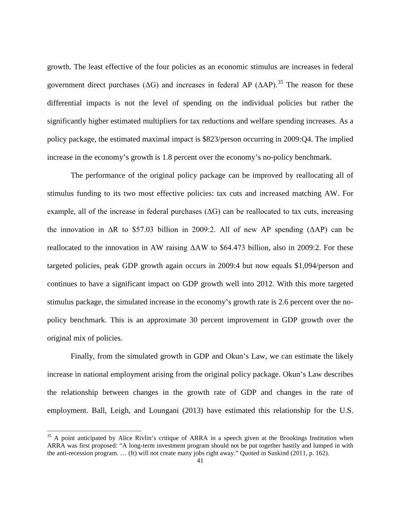
41

growth. The least effective of the four policies as an economic stimulus are increases in federal

government direct purchases (ΔG) and increases in federal AP (ΔAP).35 The reason for these

differential impacts is not the level of spending on the individual policies but rather the

significantly higher estimated multipliers for tax reductions and welfare spending increases. As a

policy package, the estimated maximal impact is $823/person occurring in 2009:Q4. The implied

increase in the economy’s growth is 1.8 percent over the economy’s no-policy benchmark.

The performance of the original policy package can be improved by reallocating all of

stimulus funding to its two most effective policies: tax cuts and increased matching AW. For

example, all of the increase in federal purchases (ΔG) can be reallocated to tax cuts, increasing

the innovation in ΔR to $57.03 billion in 2009:2. All of new AP spending (ΔAP) can be

reallocated to the innovation in AW raising ΔAW to $64.473 billion, also in 2009:2. For these

targeted policies, peak GDP growth again occurs in 2009:4 but now equals $1,094/person and

continues to have a significant impact on GDP growth well into 2012. With this more targeted

stimulus package, the simulated increase in the economy’s growth rate is 2.6 percent over the no-

policy benchmark. This is an approximate 30 percent improvement in GDP growth over the

original mix of policies.

Finally, from the simulated growth in GDP and Okun’s Law, we can estimate the likely

increase in national employment arising from the original policy package. Okun’s Law describes

the relationship between changes in the growth rate of GDP and changes in the rate of

employment. Ball, Leigh, and Loungani (2013) have estimated this relationship for the U.S.

35 A point anticipated by Alice Rivlin’s critique of ARRA in a speech given at the Brookings Institution when ARRA was first proposed: “A long-term investment program should not be put together hastily and lumped in with the anti-recession program. … (It) will not create many jobs right away.” Quoted in Suskind (2011, p. 162).

42

economy and find that a 1 percent increase in GDP implies a 0.5 percent increase in the rate of

employment. The employment level of the U.S. economy at the time of the introduction of

proposed policies (January 2009) was 142 million workers. The original policy would imply a

1.8 percent increase in GDP after one year or, by Okun’s Law, a nine-tenths of 1 percent increase

in employment. That would be 1.3 million new jobs. The more targeted stimulus policy using

only tax cuts and AW implies a 2.6 percent rate of income growth after one year, and by Okun’s

Law, a 1.3 percent increase in employment. This would be an increase of 1.85 million jobs. And

the cost per job? The total cost of the original stimulus over the year 2009:1 to 2010:1 for all four

policies was $112.82 billion. Thus the cost per job for the original ARRA policies is $86,700 per

job. For the more “efficient” targeted policy package, the cost falls to $61,000 per job.

VI. Conclusion: What Role for States?

The received wisdom, at least since Musgrave (1959) and Oates (1972), is that state

governments have little role to play in the design and implementation of macroeconomic fiscal

policy. The argument comes from either of two assumptions. First, as small open economies,

state governments cannot impact their own economies through the use of expansionary fiscal

policies. The summary in Section II of our work in Carlino and Inman (2013) rejects this

assumption. Increases in a state’s own deficits can stimulate state job growth. Or second, if there

are job gains for any one state, there may also be significant job spillovers for their neighboring

states. Our work in Carlino and Inman (2013), and the work of others studying policy

interdependencies among central European economies, finds strong support for the presence of

spillovers. If so, states may underprovide the socially efficient level of deficit policies, hoping

43

their neighbors will incur the costs of job creation. In this case, central government fiscal policies

will be needed to internalize the relevant externalities.

That said, states may still be needed. In mature economic unions, states are the main

providers of most government goods and services (defense is the exception) and often play a

central role in the financing and provision of transfers and services to lower income households.

If so, then for the central government to increase aggregate government purchases or to transfer

income to lower income households it must “use” the states. There remains a role for states, but

now as the economic “agents” of the central government. The central government may

“command” state fiscal policies, but more often than not (or because U.S. law does not allow

unfunded mandates) the central government must “control” state behavior through the use of

intergovernmental transfers. In Sections III and IV, we study the ability of such transfers to

impact state fiscal policies and to ultimately stimulate income and job creation in the national

economy. We find the most effective transfer policies are incentive-based and use matching aid

to encourage general state tax relief and income and service assistance for lower-income

households.

Why then did ARRA use relatively inefficient AP? Boone, Dube, and Kaplan (2014)

suggest that AP was the “political” price required for the timely passage of ARRA by a Congress

whose members’ political futures are closely tied to the fiscal needs of their state political allies.

As a result, the poor urban states got additional AW, the richer and more rural states got

additional infrastructure aid, and everyone received more unconstrained assistance for public

education; see Inman (2010). Here then, may be the most important role for states in

44

macroeconomic policymaking in economic unions: not just as agents for implementing approved

policies– but also as principals who collectively design these policies.

45

REFERENCES Agarwal, S., C. Liu, and N. Souleles (2007), “The Reaction of Consumer Spending and Debt to Tax Rebates – Evidence from Consumer Credit Data,” Journal of Political Economy, Vol. 115 (December), 986–1019. Arellano, M., and S. Bond (1991), “Some Tests of Specification for Panel Data: Monte Carlo Evidence and an Application to Employment Equations,” Review of Economic Studies, Vol. 58 (April), 277–297. Auerbach, A. (2003), “Fiscal Policy, Past and Present,” Brookings Papers on Economic Activity, Vol. 34 (1), 75–138. Auerbach, A., and Y. Gorodnichenko (2013), “Output Spillovers from Fiscal Policy,” American Economic Review, Vol. 103 (May), 141–146. Ball, L., D. Leigh, and P. Loungani (2013), “Okun’s Law: Fit at Fifty?” NBER Working Paper 18668, National Bureau of Economic Research. Barro, R. (1974), “Are Government Bonds New Wealth?” Journal of Political Economy, Vol. 82 (December), 1095–1117. Barro, R., and C. J. Redlick (2011), “Macroeconomic Effects of Government Purchases and Taxes,” Quarterly Journal of Economics, Vol. 126 (February), 51–102. Beetsma, R., and M. Giuliodori (2011), “The Effects of Government Purchase Shocks: Review and Estimates for the EU,” Economic Journal, Vol. 121 (February), F4–F32. Berry, W., R. Fording, E. Ringquist, R. Hanson, and C. Klarner (2010), “Measuring Citizen and Government Ideology in the U.S. States: A Re-appraisal,” State Politics and Policy Quarterly, Vol. 10 (Summer), 117–135. Blanchard, O., and R. Perotti (2002), “An Empirical Characterization of the Dynamic Effects of Changes in Government Spending and Taxes on Output,” Quarterly Journal of Economics, Vol. 117 (November), 1329–1368. Boadway, R., and A. Shah (2009), Fiscal Federalism: Principles and Practice in Multiorder Governance, Cambridge University Press. Boone, C., A. Dube, and E. Kaplan (2014), “The Political Economy of Discretionary Spending: Evidence from the American Recovery and Reinvestment Act,” Brookings Papers on Economic Activity, Vol. 48 (Spring), 375–428.

46

Bronars, S., and D. Jansen (1987), “The Geographic Distribution of Unemployment Rates in the United States: A Spatial-Time Series Analysis,” Journal of Econometrics, Vol. 36 (November), 252–279. Carlino, G., and R. P. Inman (2013), “Local Deficits and Local Jobs: Can U.S. States Stabilize Their Own Economies?” Journal of Monetary Economics, Vol. 60 (July), 517–530. Carlino, G., and R. P. Inman (2014), “A Narrative Analysis of Post World War II Changes in Federal Aid,” Working Paper 12-23/R, Federal Reserve Bank of Philadelphia. Caselli, F., G. Esquivel, and F. Lefort (1996), “Reopening the Convergence Debate: A New Look at Cross-Country Growth Empirics,” Journal of Economic Growth, Vol. 1 (September), 363–389. Chernick, H. (1998), “Fiscal Effects of Block Grants for the Needy: An Interpretation of the Evidence,” International Tax and Public Finance, Vol. 5 (May), 205–233. Chodorow-Reich, G., L. Feiveson, A. Liscow, and W. Woolston (2012), “Does State Fiscal Relief During Recessions Increase Employment? Evidence from the American Recovery and Reinvestment Act,” American Economic Journal: Economic Policy, Vol. 4 (August), 118–145. Clemens, J., and S. Miran (2012), “Fiscal Policy Multipliers on Subnational Government Spending,” American Economic Journal: Economic Policy, Vol. 4 (May), 46–68. Congressional Budget Office (CBO) (2010), “Estimated Impact of the American Recovery and Reinvestment Act on Employment and Economic Output from January 2010 Through March 2010,” May 2010, Washington, D.C. Conley, T., and B. Dupor (2013), “The American Recovery and Reinvestment Act: Solely a Government Jobs Program?” Journal of Monetary Economics, Vol. 60 (July), 535–549. Craig, S. G., and R. P. Inman (1982). “Federal Aid and Public Education: An Empirical Look and the New Fiscal Federalism,” Review of Economics and Statistics, Vol. 64 (November), 541–552. Crone, T. M. (2005), “An Alternative Definition of Economic Regions in the United States Based on Similarities in State Business Cycles,” Review of Economics and Statistics, Vol. 87 (August), 617–626. Feyrer, J., and B. Sacerdote (2011), “Did the Stimulus Stimulate? Real Time Estimates of the Effects of the American Recovery and Reinvestment Act,” NBER Working Paper 16759, National Bureau of Economic Research.

47

Finkelstein, A., S. Taubman, B. Wright, M. Bernstein, J. Gruber, J. P. Newhouse, H. Allen, and K. Baicker (2012), “The Oregon Health Insurance Experiment: Evidence from the First Year,” Quarterly Journal of Economics, Vol. 127 (August), 1057–1106. Follette, G., and B. Lutz (2010), “Fiscal Policy in the United States: Automatic Stabilizers, Discretionary Fiscal Policy Actions, and the Economy,” Finance and Economics Discussion Series, 2010-43, Federal Reserve Board. Gramlich, E. (1978), “State and Local Budgets the Day After It Rained: Why Is the Surplus So High?” Brookings Papers on Economic Activity, Vol. 9(1), 191–216. Gramlich, E. (1979), “Stimulating the Macro Economy Through State and Local Governments,” American Economic Review, Vol. 69 (May), 180–185. Grunwald, M. (2012), The New New Deal: The Hidden Story of Change in the Obama Era, New York: Simon and Schuster. Hall, R. E., and P. R. Milgrom (2008), “The Limited Influence of Unemployment on the Wage Bargain,” American Economic Review, Vol. 98 (September), 1653–1674. Hebous, S., and T. Zimmermann (2013), “Estimating the Effects of Coordinated Fiscal Actions in Euro Zone,” European Economic Review, Vol. 58 (February), 110–121. Heller, W. W. (1966), New Dimensions in Political Economy, Harvard University Press: Cambridge, MA. Holtz-Eakin, D., W. Newey, and H. Rosen (1988), “Estimating Vector Autoregressions with Panel Data,” Econometrica, Vol. 56 (November), 1371–1395. Im, K. S., M. H. Pesaran, and Y. Shin (2003), “Testing for Unit Roots in Heterogeneous Panels,” Journal of Econometrics, Vol. 115 (July), 53–74. Inman, R. P. (2008), “The Flypaper Effect,” NBER Working Paper 14579, National Bureau of Economic Research. Inman, R. P. (2010), “States in Fiscal Distress,” Regional Economic Development, Federal Reserve Bank of St. Louis, Vol. 6 (1), 65–80. Keith, R., and A. Schick (2004), “Introduction to the Federal Budget Process,” Congressional Research Service, 98-721 GOV (updated, December 28, 2004).

48

Knight, B. (2002), “Endogenous Federal Grants and Crowd-Out of State Government Spending: Theory and Evidence from the Federal Highway Aid Program,” American Economic Review, Vol. 92 (March), 71–92. Ladd, H. (1993), “State Responses to the TRA86 Revenue Windfalls: A New Test of the Flypaper Effect,” Journal of Policy Analysis and Management, Vol. 12 (Winter), 82–103. Leduc, S., and D. Wilson (2013), “Are State Governments Roadblocks to Federal Stimulus? Evidence from Highway Grants in the 2009 Recovery Act,” Working Paper Series 2013-16, Federal Reserve Bank of San Francisco. Mertens, K., and M. O. Ravn (2014), “A Reconciliation of SVAR and Narrative Estimates of Tax Multipliers,” Journal of Monetary Economics, Vol. 68 (December), S1-S19. Musgrave, R. A. (1959), The Theory of Public Finance: A Study in Public Economy, New York: McGraw-Hill. Oates, W. E. (1972), Fiscal Federalism, New York: Harcourt, Brace, Jovanovich. Ramey, V. (2011), “Can Government Purchases Stimulate the Economy?” Journal of Economic Literature, Vol. 49 (September), 673–685. Reinhart, C. M., and K. S. Rogoff (2009), “The Aftermath of Financial Crises,” NBER Working Paper 14656, National Bureau of Economic Research. Reischauer, R. (1975), “General Revenue Sharing: The Program’s Incentives,” in W. Oates (ed.), Financing the New Federalism: Revenue Sharing, Conditional Grants, and Taxation, Baltimore: Johns Hopkins University Press. Romer, C., and J. Bernstein (2009), “The Job Impact of the American Recovery and Reinvestment Plan,” Available at http://otrans.3cdn.net/ee40602f9a7d8172b8_ozm6bt5oi.pdf. Romer, C., and D. Romer (2010), “The Macroeconomic Effects of Tax Changes: Estimates Based on a New Measure of Fiscal Shocks,” American Economic Review, Vol. 100 (June), 763–801. Rossi, B., and S. Zubairy (2011), “What Is the Importance of Monetary and Fiscal Shocks in Explaining US Macroeconomic Fluctuations?” Journal of Money, Credit and Banking, Vol. 43 (6), 1247–1270. Singhal, M. (2008), “Special Interest Groups and the Allocation of Public Funds,” Journal of Public Economics, Vol. 92 (April), 548–564.

49

Shoag, D. (2013), “Using State Pension Shocks to Estimate Fiscal Multipliers since the Great Depression,” American Economic Review: Papers and Proceedings, Vol. 103 (May), 121–124. Suskind, R. (2011), Confidence Men: Wall Street, Washington, and the Education of a President, New York: Harper. United States Department of Transportation (2007), Financing Federal-Aid Highways, Publication No. FHWA-PL-07-017, March. Wilson, D. (2012), “Fiscal Spending Jobs Multipliers: Evidence from the 2009 American Recovery and Reinvestment Act,” American Economic Journal: Economic Policy, Vol. 4 (August), 251–282.

50

TABLE 1: Economic Regions

ECONOMIC REGIONS MEMBER STATES

New England Maine, New Hampshire, Vermont, Massachusetts, Rhode Island, Connecticut

Mideast New York, New Jersey, Pennsylvania, Delaware, Maryland

Southeast Virginia, North Carolina, South Carolina, Georgia, Florida, Kentucky, Tennessee,

Alabama, Mississippi, Arkansas

Great Lakes West Virginia, Michigan, Ohio, Indiana, Illinois, Wisconsin, Minnesota

Plains Missouri, Kansas, Nebraska, Iowa

Mountain/Northern Plains South Dakota, North Dakota, Montana, Idaho

Energy Belt Louisiana, Wyoming, Utah, Colorado, Texas, Oklahoma, New Mexico

Far West Arizona, California, Nevada, Oregon, Washington

Note: Economic regions are defined as in Crone (2005). Crone’s economic regions differ from the Bureau of Economic Analysis (BEA) definitions by moving West Virginia into the Great Lakes region and Louisiana into the “Energy Belt” region, both from the BEA’s Southeast region. Minnesota is added to the Great Lakes region from the BEA’s Plains region. South Dakota and North Dakota are moved to a new Mountain/Northern Plains region from the BEA’s Plains region. Wyoming, Utah, and Colorado are moved to the “Energy Belt” region from BEA’s Rocky Mountain States region. Finally, Arizona is moved to the Far West region from the BEA’s Southwest region. The BEA’s Southwest region is now omitted.

51

TA

BL

E 2

: Sta

tes’

Ow

n D

efic

its, S

tate

Job

s, an

d th

e B

enef

its o

f Coo

pera

tion:

One

Yea

r Im

pact

Eff

ects

R

EGIO

N

NEW

EN

GLA

ND

M

IDEA

ST

SOU

THEA

ST

GR

EAT

LAK

ES

PLA

INS

MO

UN

TAIN

N

OR

TH P

LAIN

S EN

ERG

Y

BEL

T FA

R

WES

T

LAR

GES

T JO

BS

STA

TE

(ΔD

efic

it/O

wn

Rev

)

Mas

sach

uset

ts

(.0

6)

New

Yor

k

(.07)

Flor

ida

(.1

5)

Illin

ois

(.11)

Mis

sour

i

(.14)

Idah

o (.1

2)

Texa

s

(.11)

Cal

iforn

ia

(.1

0)

LAR

GE

STA

TE’S

O

WN

JOB

S

(Def

icit

Cos

t/Job

)

35

,253

($

72,1

03)

95

,237

($

79,0

63)

81

,337

($

89.4

67)

63

,294

($

78,8

51)

29

,831

($

77,9

34)

6,

850

($88

,502

)

11

3,56

3 ($

85,1

75)

15

8,48

3 ($

90,9

56)

JOB

SPI

LLO

VER

S

TO O

THER

STA

TES

(Def

icit

Cos

t/Job

)

24

,149

($

0)

65

,237

($

0)

55

,716

($

0)

43

,356

($

0)

20

,434

($

0)

4,

692

($0)

77

,791

($

0)

10

8,56

1 ($

0)

REG

ION

’S T

OTA

L JO

BS

(Def

icit

Cos

t/Job

)

59

,402

($

42,7

91)

16

0,47

5 ($

46,9

22)

13

7,05

3 ($

53,0

78)

10

6,65

0 ($

46,7

96)

50

,265

($

46,2

51)

11

,542

($

52,5

23)

19

1,35

4 ($

50,5

49)

26

7,04

3 ($

53,9

80)

OTH

ER S

TATE

S’

OW

N JO

BS

(Def

icit

Cos

t/Job

)

40

,086

($

76,7

24)

13

7,92

6 ($

79,2

99)

24

2,88

1 ($

84,8

19)

19

9,41

6 ($

79,5

74)

41

,730

($

71,7

59)

13

,201

($

72,5

56)

88

,759

($

81,2

94)

90

.301

($

84,2

34)

JOB

SPI

LLO

VER

S TO

LA

RG

EST

STA

TE

(Def

icit

Cos

t/Job

)

15

,286

($

0)

48

,756

($

0)

46

,429

($

0)

38

,907

($

0)

14

,936

($

0)

3,

965

($0)

37

,577

($

0)

43

,836

($

0)

REG

ION

’S T

OTA

L JO

BS

(Def

icit

Cos

t/Job

)

67

,544

($

45,5

34)

23

2,40

6 ($

47,0

61)

40

9.25

4 ($

47,0

61)

33

6,01

5 ($

47,2

25)

70

,315

($

42,5

87)

22

,245

($

43,0

57)

14

9,55

9 ($

48,2

45)

15

2,15

8 ($

49,9

90)

REG

ION

AL

POLI

CY

JO

BS

(Def

icit

Cos

t/Job

)

12

6,94

6 ($

44,2

50)

39

2,88

1 ($

47,0

04)

54

6,30

7 ($

51,0

25)

44

2,66

5 ($

47,1

21)

12

0,58

0 ($

44,1

14)

33

,787

($

46,2

93)

34

0,91

3 ($

49,5

38)

41

9,20

1 ($

52,5

32)

Sou

rce:

Car

lino

and

Inm

an (2

013)

52

TA

BL

E 3

: SV

AR

Est

imat

es: G

DP

Res

pons

es to

Fis

cal S

hock

s for

Bla

ncha

rd a

nd P

erot

ti an

d A

id S

peci

ficat

ions

Sp

ecifi

catio

n Sa

mpl

e Pe

riod

Bla

ncha

rd a

nd

Pero

tti

1947

:1 to

201

0:3

(1)

Bla

ncha

rd a

nd

Pero

tti

1947

:1 to

201

0:3

(2)

Bla

ncha

rd a

nd

Pero

tti

1960

:1 to

201

0:3

(3)

Bla

ncha

rd a

nd

Pero

tti

1960

:1 to

201

0:3

(4)

Aid

Spe

cific

atio

n 19

60:1

to 2

010:

3 (5

)

Aid

Spe

cific

atio

n 19

60:1

to 2

010:

3 (6

)

Aid

Spe

cific

atio

n 19

60:1

to 2

010:

3 (7

)

Fisc

al P

olic

y (R

− A

) G

(R

− A

) G

R

G

A

IMPA

CT

−1.

603*

( −

1.72

, −

1.47

) .9

44*

(.94,

.947

) −

1.68

3*

( −1.

98, −

1.55

) .9

59*

(.95,

.96)

−

2.80

4*

( −2.

84, −

2.77

) .5

64*

(.56,

.57)

.5

28*

(.52,

.53)

4 Q

trs

−1.

943*

( −

2.24

, −

1.65

) .7

72*

(.46,

1.0

8)

−2.

089*

( −

2.45

, −

1.72

) 1

.000

* (.5

9, 1

.40)

−

3.28

7*

( −3.

90, −

2.67

) .4

47

( −.2

4, 1

.13)

.7

13*

(.56,

.86)

8 Q

trs

−1.

222*

( −

1.57

, −

.87)

.2

94

( −.0

7, .6

6)

−1.

223*

( −

1.70

, −

.75)

.6

19

(.20,

1.0

3)

−2.

186*

( −

2.96

, −

1.41

) .4

04

( −.3

0, 1

.11)

.4

99*

(.33,

.67)

12 Q

trs

−.6

98

( −1.

06, −

.34)

.0

23

( −.3

6, .4

1)

−.5

78

( −1.

05, −

.11)

.3

40

( −.1

1, .7

5)

−

1.50

3*

( −2.

26, −

.74)

.3

09

( −.4

4, 1

.06)

.3

60*

(.18,

.54)

20 Q

trs

−.2

35

( −.4

7, .0

6)

−.0

71

( −.3

8, .2

4)

−.0

962

( −.3

4, .1

6)

.058

( −

.38,

.50)

−

.920

( −

1.61

, −

.23)

.1

65

( −.6

4, .9

8)

.234

(.0

4, .4

3)

Peak

−

2.10

5* (Q

2)

(−

2.35

, −

1.86

) .9

63*

(Q2)

(.7

7, 1

.17)

−

2.26

7* (Q

2)

(−

2.55

, −

1.99

) 1

.078

* (Q

2)

(.67,

1.4

1)

−

3.75

5* (Q

2)

(−

4.22

, −

3.29

) .5

64*

(Q1)

(.5

6, .5

7)

.802

* (Q

2)

(.68,

.93)

N

ote:

For

Col

umns

(1)

– (

4), f

eder

al n

et r

even

ues

less

tota

l fed

eral

aid

to th

e SL

sec

tor

(R −

A)

is o

rder

ed f

irst,

then

fed

eral

gov

ernm

ent

purc

hase

s (G

), th

en G

DP.

For

Col

umns

(5)

–(7)

, the

iden

tifyi

ng o

rder

ing

is f

eder

al n

et r

even

ues

for

hous

ehol

ds a

nd f

irms

(R),

then

fed

eral

pu

rcha

ses

(G),

then

tota

l fed

eral

aid

to th

e SL

sec

tor (

A),

and

final

ly G

DP

(see

the

Tech

nica

l App

endi

x). E

ach

cell

give

s th

e po

int e

stim

ates

of

the

fisca

l mul

tiplie

r im

pact

ing

GD

P ev

alua

ted

at th

e sa

mpl

e m

eans

for

the

fisca

l var

iabl

es a

nd G

DP,

and

then

the

low

er a

nd u

pper

bou

nds

(with

in p

aren

thes

es) f

or th

e on

e st

anda

rd d

evia

tion

(68

perc

ent)

erro

r ban

d. M

ultip

liers

that

are

sig

nific

antly

diff

eren

t fro

m 0

at t

he 9

5 pe

rcen

t le

vel o

f con

fiden

ce a

re in

dica

ted

by a

n *.

53

TABLE 4: SVAR Estimates: GDP Response to Fiscal Shocks with Disaggregated Aid Specification

Sample Period 1960:1 to 2010:3 (1)

1960:1 to 2010:3 (2)

1960:1 to 2010:3 (3)

1960:1 to 2010:3 (4)

Identification Strategy SVAR SVAR SVAR SVAR

Fiscal Policy R G AP AW

IMPACT − 2.955* (−3.06, − 2.91)

.807* (.80, .82)

− .108* (− .11, − .11)

1.637* (1.61, 1.66)

4 Qtrs −3.189* (−3.71, − 2.67)

.884 (.27, 1.51)

.919 (.02, 1.78)

2.108* (1.80, 2.42)

8 Qtrs −2.067* (−2.73, − 1.40)

.677 (.07, 1.28)

.908 (.05, 1.77)

1.453* (1.07, 1.83)

12 Qtrs −1.312* (−1.97, − .067)

.498 (− .15, 1.15)

.886 (− .03, 1.80)

.988* (.58, 1.40)

20 Qtrs − .647 (−1.15, − .14)

.301 (− .40, 1.01)

.843 (− .16, 1.84)

.548 (.15, .95)

Peak −3.604* (Q2) (−3.98, − 3.23)

.884 (Q4) (.27, 1.50)

1.005 (Q2) (.19, 1.82)

2.315* (Q2) (2.08, 2.55)

Note: The initial SVAR identification used here orders federal net revenues (R) first, then federal government purchases (G), then welfare aid (AW), then general revenue/project aid (AP), and finally GDP; see the Technical Appendix. Each cell gives the point estimates of the fiscal multiplier impacting GDP evaluated at the sample means for each fiscal variable and GDP, and then the lower and upper bounds (within parentheses) for the one standard deviation (68 percent) error band. Multipliers that are significantly different from 0 at the 95 percent level of confidence are indicated by an *.

54

TA

BL

E 5

: SV

AR

Est

imat

es: R

obus

tnes

s

Spec

ifica

tion

Sa

mpl

e Pe

riod

α r,y

= 3

.0

1960

:1 to

20

10:3

(1

)

α r,y

= 3

.0

1960

:1 to

20

10:3

(2

)

Ord

erin

g 19

60:1

to

2010

:3

(3)

Ord

erin

g 19

60:1

to

2010

:3

(4)

With

Mon

etar

y 19

60:1

to

2010

:3

(5)

With

Mon

etar

y 19

60:1

to

2010

:3

(6)

No

Settl

emen

t 19

60:1

to

1998

:3

(7)

No

Settl

emen

t 19

60:1

to

1998

:3

(8)

Iden

tific

atio

n St

rate

gy

SVA

R

SVA

R

SVA

R

SVA

R

SVA

R

SVA

R

SVA

R

SVA

R

Fisc

al P

olic

y A

P A

W

AP

AW

A

P A

W

AP

AW

IMPA

CT

−

.076

* ( −

.08,

−.0

7)

1.14

6*

(1.1

3, 1

.17)

−

.109

* ( −

.10,

−.1

2)

1.5

94*

(1.5

7, 1

.62)

−

.096

* ( −

.09,

−.1

0)

1.6

42*

(1.6

3, 1

.65)

−

.002

* ( −

.003

, −

.001

) 1.

584*

(1

.56,

1.6

1)

4 Q

trs

.954

(.1

0, 1

.81)

1.

577*

(1

.33,

1.8

2)

.930

(.0

6, 1

.80)

1

.882

* (1

.62,

2.1

5)

.244

(.0

9, .4

0)

1.5

11*

(1.2

9, 1

.78)

.6

24

(.06,

1.7

8)

2.04

0*

(1.7

4, 2

.34)

8 Q

trs

.930

(.0

7, 1

.79)

1.

109*

(.8

2, 1

.39)

.9

18

(.05,

1.7

9)

1.2

53*

(.91,

1.5

9)

.293

(.1

32, .

455)

.4

27

(.11,

.75)

.9

08

(.05,

1.7

6)

1.40

7*

(.89,

1.7

7)

12 Q

trs

.899

( −

.02,

1.8

1)

.769

* (.4

5, 1

.08)

.8

96

( −.0

3, 1

.82)

.8

09*

(.44,

1.1

8)

.172

( −

.00,

.35)

–.

137

( −.4

6, .1

8)

.885

( −

.03,

1.80

) .9

56*

(.56

1.35

)

20 Q

trs

.850

( −

.15,

1.8

5)

.441

(.1

2, .7

6)

.853

( −

.16,

1.8

7)

.392

( −

.07,

.718

) −

.110

( −

.29,

.07)

−

.213

( −

.46,

.04)

.8

50

( −.1

5, 1

.84)

.5

31

( −.1

5, .9

2)

Peak

.9

69 (Q

3)

(.12,

1.8

2)

1.71

5* (Q

2)

(1.5

2, 1

.91)

1.

017

(Q2)

(.2

0, 1

.84)

2.

068*

(Q2

) (1

.88,

2.2

6)

.305

(Q7)

(.1

5, .4

6)

2.00

0* (Q

2)

(1.7

9, 2

.21)

1.

005

(Q2)

(.1

9, 1

.82)

2.

242*

(Q2)

(2

.01,

2.4

7)

N

ote:

All

resu

lts a

re f

or s

ampl

e pe

riod,

196

0:1

to 2

010:

3. C

olum

ns (

1) a

nd (

2) u

se a

mor

e el

astic

coe

ffic

ient

spe

cify

ing

the

auto

mat

ic (

sam

e qu

arte

r) i

mpa

ct o

f G

DP

on f

eder

al n

et r

even

ues.

Col

umns

(3)

and

(4)

allo

w f

or m

onet

ary

polic

y va

riabl

es (

fede

ral

fund

s ra

te a

nd r

ate

of

infla

tion)

with

in th

e SV

AR

spec

ifica

tion

with

fisc

al p

olic

y or

dere

d be

fore

mon

etar

y po

licy.

Col

umns

(5) a

nd (6

) rep

ort r

esul

ts fo

r the

alte

rnat

ive

orde

ring

of g

over

nmen

t fis

cal p

olic

y w

ith g

over

nmen

t spe

ndin

g (G

and

AP)

ord

ered

firs

t, th

en r

even

ue p

olic

ies

(R, A

W),

follo

wed

by

GD

P.

Col

umns

(7) a

nd (8

) rep

ort r

esul

ts fo

r the

rest

ricte

d sa

mpl

e pe

riod,

196

0:1

to 1

998:

3 ex

clud

ing

the

Toba

cco

Settl

emen

t and

sub

sequ

ent q

uarte

rs.

Each

cel

l giv

es th

e po

int e

stim

ates

of t

he fi

scal

mul

tiplie

r im

pact

ing

GD

P ev

alua

ted

at th

e sa

mpl

e m

eans

for f

isca

l pol

icie

s an

d G

DP,

and

then

th

e lo

wer

and

upp

er b

ound

s (w

ithin

par

enth

eses

) fo

r th

e on

e st

anda

rd d

evia

tion

(68

perc

ent)

erro

r ba

nd.

Mul

tiplie

rs t

hat

are

sign

ifica

ntly

di

ffere

nt fr

om 0

at t

he 9

5 pe

rcen

t lev

el o

f con

fiden

ce a

re in

dica

ted

by a

n *.

55

TA

BL

E 6

: Sta

te B

udge

tary

Res

pons

es to

Fed

eral

Aid

: 197

9 to

201

0

rs

[$30

63]

(1)

b [$

276]

(2

)

gs

[$30

03]

(3)

k [$

312]

(4

)

Δc

[$81

] (5

)

Δd

[$55

] (6

)

Δf

[−

$50]

(7

)

I

[$60

,566

] .0

24*

(.00

2)

.002

*

(.0

005)

.0

12*

(.00

2)

.001

*

(.

0005

) .0

06*

(.0

01)

.001

(.0

01)

≡ .0

04

AP

[$50

4]

−.0

00

(.05

2)

.006

(.0

10)

.379

*

(.

041)

.1

27*

(.0

16)

.326

*

(.064

) .0

33

(.048

) ≡

.195

c -1

[$24

85]

.021

*

(.

010)

.0

06*

(.00

2)

.059

*

(.

009)

.0

10*

(.0

03)

−.1

07*

(.0

11)

−.0

36*

(.008

) ≡

.017

( 1−

m)

[.39]

52

5.8*

(2

24.0

) 40

5.9*

(7

5.1)

45

7.0*

(2

15.0

) 75

.66

(66

.67)

−

7.01

(2

18.7

) 15

2.9

(160

.7)

≡ −

253

N

1536

15

36

1536

15

36

1536

15

36

153

6

R2

.93

.81

.94

.76

.20

.12

NA

N

ote:

Bud

get e

quat

ions

rep

orte

d in

col

umns

(1)

to (

7) a

re e

stim

ated

by

gene

raliz

ed le

ast s

quar

es a

llow

ing

for

stat

e-sp

ecifi

c A

R(1

) pr

oces

ses.

Het

eros

keda

stic

-cor

rect

ed s

tand

ard

erro

rs a

re re

porte

d w

ithin

par

enth

eses

; coe

ffic

ient

s tw

ice

thei

r sta

ndar

d er

rors

are

indi

cate

d by

an

*. C

olum

n (7

) re

ports

the

impl

ied

impa

ct o

f eac

h in

depe

nden

t var

iabl

e re

quire

d fo

r bu

dget

ary

“add

ing

up”

for

the

resi

dual

cat

egor

y “n

et c

ontri

butio

ns to

tru

st fu

nd a

ccou

nts”

den

oted

as

Δf (≡

AP

+ rs

−

(b +

gs

+ k)

−

Δc

+ Δd

). In

add

ition

to I,

AP,

(1−

m),

and

c -1,

each

regr

essi

on a

lso

incl

udes

as

inde

pend

ent v

aria

bles

: yea

r and

stat

e fix

ed e

ffec

ts p

lus

stat

e-ye

ar c

ontro

ls fo

r the

cos

t of l

ivin

g in

the

stat

e; c

itize

n pr

efer

ence

s m

easu

red

on a

lib

eral

-con

serv

ativ

e sp

ectru

m; t

he st

ate’

s rep

ublic

an v

ote

in th

e pr

evio

us p

resi

dent

ial e

lect

ion;

a (1

,0) i

ndic

ator

var

iabl

e fo

r whe

ther

the

budg

et is

de

cide

d in

an

elec

tion

year

for

gov

erno

r; a

(1,0

) in

dica

tor

varia

ble

for

the

pres

ence

of

a st

ate

rain

y-da

y fu

nd r

equi

rem

ent;

natio

nal o

il pr

ice

shoc

ks in

tera

cted

with

regi

onal

indi

cato

r var

iabl

es fo

r con

sum

ing

stat

es in

New

Eng

land

, Gre

at L

akes

, and

the

Mid

-Eas

t or p

rodu

cing

sta

tes

in

the

Sout

hwes

t an

d R

ocky

Mou

ntai

n re

gion

s; s

hock

s to

sta

te m

ilita

ry c

ontra

cts

and

payr

oll;

and

the

lagg

ed l

evel

of

real

per

cap

ita p

rope

rty

dam

ages

with

in th

e st

ate

caus

ed b

y “b

illio

n do

llar”

nat

ural

dis

aste

rs, a

nd s

hock

s to

the

stat

e un

empl

oym

ent r

ate.

Sam

ple

mea

ns a

re li

sted

bel

ow

each

var

iabl

e.

56

TA

BL

E 7

: Sim

ulat

ed F

our

Qua

rter

Fis

cal M

ultip

lier

for

Fede

ral P

roje

ct A

id

Fo

r a $

1 In

crea

se in

Fed

eral

Pro

ject

Aid

: ΔAP

= 1

Δrs

= .0

00

ΔB

= Δ

b/(1−

m) Δ

G =

Δgs

+ Δ

k

ΔW =

Δ

c −

Δd

+ Δ

f

Δrs

= .0

00

.01

5 =

.006

/(1 −

.6)

.506

= .3

79 +

.127

.48

8 =

.326

− .0

33 +

.195

For a

$1

Incr

ease

in F

eder

al P

roje

ct A

id: Δ

AP =

1*

Δr

s/ΔA

P ≃

.00

ΔB

/ΔA

P ≃

.02

ΔG

/ΔA

P ≃

.50

ΔW/Δ

AP ≃

.48

Si

mul

ated

Fou

r Qua

rter

Pro

ject

Aid

(AP)

Mul

tiplie

r

dGD

P/dA

P =

(dG

DP/

drs)

∙[Δrs

/ΔA

P] +

(dG

DP/

dB)∙[

ΔB/Δ

AP]

+ (d

GD

P/dG

)∙[ΔG

/ΔA

P] +

(dG

DP/

dW)∙[

ΔW/Δ

AP]

,

.52

=

( −

3.19

)∙[.0

00]

+

(1

.59)

∙[.02

]

+

(.8

8)∙[.

50]

+

(

.10)

∙[.48

]

* M

argi

nal e

ffec

ts o

f cha

nges

in A

P in

volv

e ro

undi

ng a

nd sa

tisfy

“ad

ding

-up”

to a

lloca

te th

e $1

of n

ew A

P as

sist

ance

.

57

TA

BL

E 8

: Sim

ulat

ed F

our

Qua

rter

Fis

cal M

ultip

lier

for

Fede

ral W

elfa

re A

id

Fo

r .10

Incr

ease

in th

e Fe

dera

l Wel

fare

Mat

chin

g Ra

te fr

om m

0 = .6

0 to

m1 −

.70

Cha

nges

in th

e O

vera

ll St

ate

Budg

et

Δr

s = −

$52.

58

Δb

= −

$40.

59

ΔG

= Δ

gs +

Δk

= −

$45.

70 +

−.$

7.60

= −

$53

.30

ΔW

= Δ

c −

Δd

+ Δ

f =

$.70

− (−

$15.

29) +

$25

.30

= $4

1.31

Cha

nges

in P

over

ty S

uppo

rt a

nd F

eder

al W

elfa

re A

id

B

0 = b

0/(1 −

m0)

= 27

6/(1

−.6

) = $

690

B1

= [b

0 + Δ

b]/(1

− m

1) =

[276

+ (−

40.5

9)]/(

1 −

.7) =

$78

5

ΔB

= B

1 −

B0 =

$78

5 −

$69

0 =

$95

ΔA

W =

Δ(W

elfa

re A

id) =

(m1)∙

(B1) −

(m0)∙

(B0)

= (.7

)∙($7

85) −

(.6)

∙($69

0) =

$54

9.50

− $

414

= $1

35.5

0

For a

$1

Incr

ease

in F

eder

al W

elfa

re A

id: Δ

AW =

1*

Δr

s/ΔA

W =

(−

52.5

8)/(1

35.5

0) =

−.3

9 Δ

B/Δ

AW

= (9

5)/(1

35.5

0) =

.70

ΔG

/ΔA

W =

(−

53.3

0)/(1

35.5

0) =

−.3

9

ΔW

/ΔA

W =

(41.

30)/(

135.

50)

= .3

0

Sim

ulat

ed F

our Q

uart

er W

elfa

re A

id (A

W) M

ultip

lier

dGD

P/dA

W =

(dG

DP/

drs)

∙[Δrs

/ΔA

W] +

(dG

DP/

dB)∙[

ΔB/Δ

AW

] + (d

GD

P/dG

)∙[ΔG

/ΔA

W] +

[dG

DP/

dW)∙[

ΔW/Δ

AW

],

2.04

=

(−

3.19

)∙[ −

.39]

+

(1.5

9)∙[.

70]

+

(

.88)

∙[ −

.39]

+

(.10)

∙[.30

] *M

argi

nal e

ffec

ts o

f cha

nges

in A

P in

volv

e ro

undi

ng a

nd sa

tisfy

“ad

ding

-up”

to a

lloca

te th

e $1

of n

ew A

P as

sist

ance

.

58

TA

BL

E 9

: Fis

cal S

timul

us a

nd S

imul

ated

GD

P G

row

th F

ollo

win

g A

RR

A

Pred

icte

d G

ains

in R

eal G

DP

Per C

apita

for A

ltern

ativ

e “F

isca

l Inn

ovat

ions

” (2

005

Dol

lars

)

PER

IOD

B

ASE

LIN

E PR

EDIC

TED

G

DP

(1)

TAX

R

ELIE

F (Δ

R)

(2)

FED

ERA

L PU

RC

HA

SES

(ΔG

) (3

)

PR

OJE

CT

A

ID

(ΔA

P)

(4)

WEL

FAR

E A

ID

(ΔA

W)

(5)

FULL

ST

IMU

LUS

(ALL

PO

LIC

IES)

(6

)

“TA

RG

ETED

” ST

IMU

LUS

(ΔR

; ΔA

W)

(7)

2009

:Q1

41,2

79

- -

- -

- -

2009

:Q2

41,6

75

604

0.00

−

0.00

11

6 72

2 97

0

2009

:Q3

41,8

87

649

0.00

12

13

6 80

0 10

62

2009

:Q4

42,1

97

659

0.00

15

14

7 82

3 10

94

2010

:Q1

42,6

40

640

23

11

141

819

1060

2010

:Q2

43,1

40

603

11

32

132

781

997

2010

:Q3

43,6

49

558

12

38

122

734

921

2010

:Q4

44,1

41

500

9 31

11

0 65

3 82

7

2011

:Q1

44,6

90

442

6 26

98

57

3 73

0

2011

:Q2

45,0

52

384

3 25

86

49

9 63

5

2011

:Q3

45,4

65

330

.1

24

74

429

547

2011

:Q4

45,8

50

280

−2

22

64

364

465

2012

:Q1

46,2

09

235

−4

19

54

306

393

2012

:Q2

46,5

44

196

−5

16

46

254

329

2012

:Q3

46,8

60

163

−7

14

39

209

273

2012

:Q4

47,1

60

134

−8

11

33

170

226

59

60

61

62

TECHNICAL APPENDIX

SVAR Specification and Identification of Fiscal Multipliers

The four-variable SVAR estimates the impact of federal net revenues paid by households

and firms (R), federal government purchases (G), and aggregate federal aid (A) on national GDP

(Y). The analysis begins with the estimation of a reduced form VAR specified as:

Zt = C(L)∙Zt-1 + ut, where (A1)

Ztʹ = [rt, gt, at, yt] and utʹ = [urt, ug

t, uat, uy

t],

and where rr is the log of federal net household and firm revenues (R), gt is the log of federal

government purchases (G), at is the log of aggregate federal aid (A), and yt is the log of GDP

(Y), each measured at quarterly intervals and measured as real (2005) dollars per capita. Also

included in the initial VAR are the trend variables time and time squared, and an indicator

variable for “deep recessions” (= 1, if the national rate of unemployment exceeds 8 percent).

The lag structure C(L) is a 4 by 4 matrix of three-quarter distributed lag polynomials, and

ut is a 4 by 1 vector of reduced form innovations, specified as utʹ = [urt, ug

t, uat, uy

t]. The three

quarter lag allows for seasonal patterns in the responses of fiscal variables to GDP. The Akaike

information criterion test statistic indicates that three quarter lags of the endogenous variables are

optimal; three-lags are also sufficient to remove serial correlation from the residuals.

To recover the exogenous structural shocks to net federal revenues, federal government

purchases, and federal aid, denoted as vrt, vg

t, and vat, respectively, we follow the methodology of

Blanchard and Perotti (2002). First, we take advantage of quarterly variation in our data and

impose the restriction that discretionary changes in fiscal policy take at least one quarter to

63

respond to changes in GDP. Thus, the contemporaneous discretionary response of net revenues,

purchases, or aid to GDP is zero.

Second, we impose constraints on the ordering of discretionary policy changes, requiring

discretionary revenues to be set prior to discretionary spending for either purchases or aid, and

then within spending, that purchases (largely defense spending) are set prior to federal aid to the

SL sector. The Congressional Budget and Impoundment Control Act of 1974 and subsequent

legislation have established aggregate revenues as the first decision for congress when setting the

federal budget; see Keith and Schick (2004) and Auerbach (2003). Formally, federal net

revenues are seen to Granger-cause federal purchases.1 We assume discretionary government

purchases predetermine spending for federal aid as, politically, defense spending “trumps”

discretionary domestic spending. We cannot rule out the possibility that domestic spending may

hold priority over defense spending by a Granger-causality test.2 As a precaution, therefore, we

redo our analysis with federal purchases pre-dating revenues in the policy process and report

those results as a robustness check in Table 5.3

Third, we identify the built-in responses of federal tax and transfer policies and federal

purchases to contemporaneous (same quarter) changes in GDP following the specifications

proposed originally by Blanchard and Perotti (2002). The built-in contemporaneous elasticity of

federal net household and firm revenues to changes in GDP is set equal to 2.08; sensitivity test

for alternative specifications are reported in Table 5. An estimate of the contemporaneous (same

1 For the full sample period (1947:1 to 2010:3), we reject the null hypothesis that revenues do not Granger-cause spending (χ2 = 14.01), but we cannot reject the null that spending does not Granger-cause revenues (χ2 = 3.84).

2 For the full sample period (1947:1 to 2010:3) we cannot reject either the null hypothesis that federal aid Granger-causes federal purchases (χ2 = 14.26) or the null hypothesis that federal purchases Granger-cause federal aid.

3 We have tested for the sensitivity of our core results to the alternative ordering within spending that places domestic spending politically “prior” to defense spending, and the results remain essentially the same.

64

quarter) built-in effects of GDP on federal aid to the SL sector is obtained from a panel

regression for the period 1970 to 2010 relating the log of total federal-to-state aid to the log of

gross state product (GSP) conditional on year and state fixed effects; our preferred elasticity

estimate is − .35 (standard error = .10).

The vector of reduced form residuals is then specified as a linear combination of

structural shocks. After subtracting all contemporaneous responses among the reduced form

residuals, net residuals (uC,∙) can be specified as:

uC,rt ≡ (ur

t − αr,y∙uyt) = βr,g∙vg

t + βr,a∙vat + vr

t,

uC,gt ≡ (ug

t − αg,y∙uyt) = βg,r∙vr

t + βg,a∙vat + vg

t,

uC,at ≡ (ua

t − αa,y∙uyt) = βa,g∙vg

t + βa,r�vrt + va

t, (A2)

uC,yt ≡ (uy

t − αy,r∙urt − αy,g∙ug

t − αy,a∙uat) = vy

t,

where each coefficient αp,y specifies the built-in (programmatic) elasticity of fiscal policy (p = r,

g, a) to GDP and each coefficient αy,p the response of GDP to contemporaneous (including

exogenous) changes in each fiscal policy ( p = r, g, a).

Our core estimates set αr,y = 2.08, αg,,y = 0, and αa,y = − .35. From the identification

strategy for the timing of fiscal policy decision-making, βr,g = βr,a = 0 from the priority of federal

revenues over spending and βg,a = 0 from the priority of government purchases over SL aid. With

these restrictions, we identify the remaining six free parameters (βg,r, βa,g, βa,r, αy,r, αy,g, αy,a) and

compute a distribution for the exogenous structural errors, vtʹ = [vrt, vg

t, vat, vy

t]. We can then

compute impulse response functions for GDP following exogenous shocks in fiscal policy drawn

from the estimated distributions of the structural errors, and then from the impulse response

functions we can estimate multipliers evaluated at the sample means for GDP and each policy;

see Table 3.

65

A similar specification and identification strategy is used when the analysis is extended to

a five-variable SVAR to evaluate the separate effects for project aid (AP) and welfare aid (AW).

Here the vector of policies and GDP is specified as Zʹ = [rt, gt, awt, apt, yt], where awt is the log

of federal matching aid for state-funded transfers to lower-income households including

Medicaid (AW) and apt is the log of federal project aid for general state and local government

spending or tax relief (AP). The corresponding vector of exogenous residuals to be estimated is

now vtʹ = [vrt, vg

t, vawt, vap

t, vyt]. The five variable SVAR is specified as:

uC,rt ≡ (ur

t − αr,y∙uyt) = βr,g∙vg

t + βr,aw∙vawt + βr,ap∙vap

t + vrt,

uC,gt ≡ (ug

t − αg,y∙uyt) = βg,r∙vr

t + βg,aw∙vawt + βg,ap∙vap

t + vgt,

uC,awt ≡ (uaw

t − αaw,y∙uyt) = βaw,rv∙rt + βaw,g∙vg

t + βaw,ap∙vapt + vaw

t, (A3)

uC,apt ≡ (uap

t − αap,y∙uyt) = βap,r∙vr

t + βap,g∙vgt + βap,aw∙vaw

t + vapt,

uC,yt ≡ (uy

t − αy,r∙urt − αy,g∙ug

t − αy,aw∙uawt − αy,ap∙uap

t) = vyt,

where we again specify αr,y = 2.08 and αg,y = 0, βr,g = βr,aw = βr,ap = 0 by the budgetary priority of

revenue over spending; and βg,aw = βg,ap = 0 from the budgetary priority of government purchases

(largely defense) over grants to the SL sector. Initially, we specify formula AW as prior in

budgeting to discretionary federal AP and set βaw,ap = 0. For the five-variable SVAR, we use

estimates of the contemporaneous built-in effects of GDP on the two components of federal aid,

again obtained from state panel regressions now relating the log of AW and AP to the log of

GSP, conditional on year and state fixed effects. Here the preferred estimates are αap,y = − .40

(s.e. = .15) and αaw,y = − .19 (s.e., =.07).4 Both sets of aid policies are progressive, increasing as

4 Explicitly including the contemporaneous effect of changes in GDP on AW and AP removes possible bias in our multiplier estimates that could arise if Congress responds to a recessionary shock with immediate additional assistance for the SL sector. Historically, Congress has introduced intergovernmental aid programs two and three years after recessions to help states cover their recession-induced shortfalls in revenue. But the fact that the lagged influence of income on policy is never statistically significant beyond three to four quarters leads us to view these programs as exogenous shocks to fiscal policy.

66

income declines. Our assumed ordering of fiscal policy again has Congress first determine

revenues, then government purchases, then AW, and finally AP. With these restrictions, we can

identify the 10 free parameters (βg,r, βaw,r, βaw,g, βap,r, βap,g, βap,aw, αy,r, αy,g, αy,aw, αy,ap) and the

resulting vector of exogenous residuals vtʹ = [vrt, vg

t, vawt, vap

t, vyt]. We can then compute the

impulse response functions for GDP following exogenous shocks in fiscal policy, and from these

impulse response functions we can estimate fiscal multipliers evaluated at the sample means for

GDP and each policy, now including those for AW and program aid AP (see Tables 4 and 5).