Geothermal Investigations in Ohio and Pennsylvania
92
LA-9223-HDR UC-66b Issued: April 1982 LA--9 223-HDR DE82 016129 Geothermal Investigations in Ohio and Pennsylvania Yoram Eckstein* Richard A. Heimlich* Donald F. Palmer* Spencer S. Shannon, Jr. * Department of Geology, Kent State University, Kent, OH 44242. Los Alamos National Laboratory Los Alamos,New Mexico 87545
Transcript of Geothermal Investigations in Ohio and Pennsylvania

LA-9223-HDR
UC-66b Issued: April 1982
LA--9 223-HDR
DE82 016129
Geothermal Investigations in Ohio and Pennsylvania
Yoram Eckstein* Richard A. Heimlich*
Donald F. Palmer* Spencer S. Shannon, Jr.
* Department of Geology, Kent State University, Kent, OH 44242.
Los Alamos National Laboratory Los Alamos,New Mexico 87545

DISCLAIMER
This report was prepared as an account of work sponsored by an agency of the United States Government. Neither the United States Government nor any agency Thereof, nor any of their employees, makes any warranty, express or implied, or assumes any legal liability or responsibility for the accuracy, completeness, or usefulness of any information, apparatus, product, or process disclosed, or represents that its use would not infringe privately owned rights. Reference herein to any specific commercial product, process, or service by trade name, trademark, manufacturer, or otherwise does not necessarily constitute or imply its endorsement, recommendation, or favoring by the United States Government or any agency thereof. The views and opinions of authors expressed herein do not necessarily state or reflect those of the United States Government or any agency thereof.

DISCLAIMER Portions of this document may be illegible in electronic image products. Images are produced from the best available original document.

GEOTHERMAL INVESTIGATIONS
IN
O H I O AND PENNSYLVANIA
Yoram Eckstein, Richard A. Heimlich, Donald F. Palmer, and Spencer S. Shannon, J r .
ABSTRACT
New values of heat flow were determined for the Appalachian Plateau i n eastern Ohio and northwestern Pennsylvania. Corrected values for wells i n Washington and Summit Counties, Ohio, a re 1.36 and 1.37 heat-flow units (HFU), respectively. Those of 1.84 and 2.00 HFU define a previously unknown heat-flow h i g h i n Venango and Clarion counties, Pennsylvania. Thermal conductivity was measured fo r core samples from 12 wells i n Ohio and 6 wells i n Pennsylvania. Heat production was determined for 34 core and outcrop samples from Ohio, Pennsylvania, and New Jersey.
INTRODUCTION
This work was undertaken as par t of a program to se l ec t s i t e s for hot, dry rock geothermal-energy extraction i n the eastern United States . In t h i s study, areas having re la t ive ly h i g h conductive heat flow associated w i t h radiogenic heat-producing plutons were sought i n Ohio and western Pennsyl- vania. From the geological and geophysical l i t e r a t u r e , the authors chose areas i n w h i c h geothermal gradients could be measured i n wells, and the thermal conductivity of core samples obtained. From these d a t a they deter- mined the conductive heat flow for four favorable s i t e s .
1

GEOLOGY
Figure 1 depicts the geometry of the Precambrian basement surface inferred from 120 wells (Owens, 1967; Saylor, 1968). Subsurface depths to Precambrian rocks range from < 0.6 km i n western Ohio to > 3.6 km i n eastern Ohio and western Pennsylvania.
The Precambrian surface i n western Ohio reveals the broad linear Indiana-Ohio platform (Green, 19571, which may be the structural predecessor of the Cincinnati-Findlay Arch. The eastern slope of the basement platform increases eastward from 1 t o 20 m/km and forms the western margin of the Appalachian Basin. The surface d i p s to the eas t i n eastern Ohio, and to the south i n northwestern Pennsylvania.
In eastern and central Ohio ( F i g . 21, and i n northwestern Pennyslvania (Saylor, 1968), samples from the basement comprise quartz-feldspar gneiss, smaller amounts of quartz-mica schist and amphibolite, and minor occurrences of marble and c a l c s i l i c a t e rocks. The western t h i r d o f Ohio seems t o be un- derlain by Precambrian quartz-feldspar gneiss and granite. Also rhyol i te , trachyte, and andesite (McCormick, 1961; Gonterman, 1973) have been ident i f ied.
I f only the rock i n the immediate subcrop is mapped, the underlying rock t h a t may have more geophysical significance is ignored. A1 though Summerson (1962) maps an area underlying Guernsey County, O h i o , as gran i t ic gneiss, only the upper 3 m are gneiss, whereas the next 81 m a re amphibolite (McCormick, 1961). In this study, the dominant lithology i s mapped and a s ingle pattern is used for medium to coarse quartzo-feldspathic rocks. The mapped area of some rock types has been decreased around dr i l l -hole s i t e s . A newly ident i - f i e d area of grani te (M. F. Schmidt, personal communication) i n Morrow County has been added to the Ohio map.
Precambrian rocks crop out only i n southeastern Pennsylvania. Granite, d i o r i t e , gabbro, and anorthosite are associated w i t h g ran i t ic gneiss, para- gneiss, and metavolcanic rocks (Gray and Shepps, 1960). Throughout the r e s t of the s t a t e they are ident i f ied from cores and cuttings and by interpretat ion of geophysical data. Rocks i n the basement i n Ohio and northwestern Pennsyl- vania a re similar to those i n Precambrian outcrops i n Pennsylvania. However, anorthosite has been reported only i n southeastern Pennsylvania.
The basement i n O h i o and western Pennsylvania may be an extension o f the Grenvil l e b e l t based on radiometric age determinations (Bass, 1960; Rudman e*;
2

Fig. 1.
Elevation o f top of Precambrian basement in Ohio and Pennsylvania (from Owens, 1967 and Saylor, 1968).
Ti! -FELDSPAR GNEISS CHYTE, ANDESITE
Fig. 2.
Precambrian rock types in Ohio and Pennsylvania (from McCormick, 1961; Summerson, 1962; Saylor, 1969; and Ross, 1972).
3

a l . , 1965; Lidiak e t a1 ., 1966; Hofmann e t a1 ., 1972; Lapham, 1975; Barbis, 1978). Rb-Sr and K-Ar ages determined on b i o t i t e and muscovite from such rocks i n Ohio and on whole rock samples from Pennsylvania range from 837 t o 942 Myr. Exceptions a re whole-rock Rb-Sr ages (1242 and 1304 Myr) fo r two Ohio trachyte and rhyol i te samples (Lidiak e t a l . , 1966; Barbis, 1978), and Rb-Sr feldspar ages for four Ohio gneiss and grani te samples, w h i c h range from 1118 t o 1406 Myr (Barbis, 1978).
Barbis (1978) concludes t h a t the Precambrian basement i n Ohio was metamorphosed during the Grenville orogeny 1171 - + 36 Myr ago. The d i s t r i b u - t ion of basement ages rules out an e a r l i e r conclusion (Bass, 1960) t h a t the Grenville Front extends southward from Canada through western Ohio. The trachyte and rhyol i te dates indicate t h a t volcanism occurred about 1280 Myr I
ago. A l l basement rocks i n Ohio and western Pennsylvania have Precambrian ages.
The Precambrian basement i s overlain by Paleozoic sedimentary rocks t h a t range i n thickness from < 0.6 km i n western Ohio t o > 5.5 km i n southeastern Pennsylvania. The Paleozoic s t ra t igraphy is described by Shearrow (1957) and Collins (1979). The dominant rock types are:
System L i tho1 ogy
Permi an Pennsylvanian Mississippian Devonian Si 1 uri an Ordovician Cambrian
Sands tone Sandstone, shale, limestone, coal Sandstone, s i l t s t o n e , shale Limestone, shale Sandstone, carbonate rocks, evaporite Carbonate rocks Sands tone
Cambrian and Ordovician sch i s t , gneiss, quar tz i te , and serpentinite crop out i n southeastern Pennsylvania. In the same area, Triassic shales and sand- stones a re in t ruded by diabase dikes. Pleistocene moraines overl ie much of the bed rock i n the northern par t s of O h i o and Pennsylvania.
s t ructural province, which includes Ohio and western In the Plateau Pennsyl van i a , f 1 a t-1 y nq Paleozoic rocks loca l ly have gentle folds. Low re- -
4

gional d ips o f t he Paleozoic rocks i n Ohio a re r e l a t e d t o the C inc inna t i Arch
(F ig . 3 ) where u p l i f t began no e a r l i e r than S i l u r i a n t ime (Scotford, 1964).
I n the Va l ley and Ridge Province i n cen t ra l Pennsylvania, the Paleozoic rocks were deformed by i n tens i ve f o l d i n g and t h r u s t f a u l t i n g . I n southeastern
Pennsylvania, t he s t r u c t u r a l features i n metamorphic rocks o f the Piedmont Province are p a r t i a l l y obscured by sedimentary and vo lcanic rocks i n T r i a s s i c
grabens.
GEOPHYSICAL SURVEYS
Sources o f g r a v i t y data inc lude surveys o f Ohio (Heiskanen and U o t i l a , 1956), Pennsylvania (Diment e t a1 ., 1972), and the Uni ted States (Woollard and
Joest ing, 1964).
The reg ion has genera l l y negat ive Bouguer g r a v i t y values t h a t are char-
a c t e r i s t i c o f cont inents . I n easternmost Ohio and western Pennsylvania there are s l i g h t f l u c t u a t i o n s i n g r a v i t y values. Prominent anomalies occur i n cen-
t r a l and western Ohio and i n cen t ra l and eastern Pennsylvania. The longer
wavelengths and more subdued anomalies i n eastern Ohio may be r e l a t e d t o the increased depth t o the basement (Rudman e t a1 ., 1965) o r t o g rea ter homogene-
i t y o f the basement rocks (Summerson, 1962). Because the basement i n western
Ohio has more g ran i te in te rspersed w i t h metamorphic rocks, dens i ty o f the t e r -
r a i n i s more heterogeneous. Pincus (1960) concluded from an ana lys is o f f i v e
major Bouguer anomalies i n Ohio t h a t they a re caused by dens i ty cont ras ts
w i t h i n t h e Precambrian basement complex. P o s i t i v e anomal i e s i n northwestern Ohio have amp1 i tudes and wave1 engths
o f 40 mgal and 25 km i n Sandusky and Seneca Counties, 10 mgal and 25 km i n
Lucas and Wood Counties, and 30 mgal and 50 km i n Auglaize, Shelby, and Miami Counties (Newhart, 1975; Haidarian, 1976; Wil l iams, 1976; and Quick, 1976). A l a r g e negat ive anomaly s tud ied by Haidar ian (1976) has an amplitude o f 25 mgal and a wavelength o f 65 km. The p o s i t i v e anomalies seem t o be r e l a t e d t o gab-
b r o o r amphibol i te masses i n the c rus t , whereas the negat ive anomaly may be r e l a t e d t o a deeper g r a n i t e p lu ton. However, t he pe t ro logy deduced from grav-
i t y values does n o t agree w i t h cores o f basement rocks (McCormick, 1961; Summerson, 1962). A1 though t h e h i gh-amp1 i tude Bouguer anomaly and magnetic
anomaly i n Sandusky and Seneca Counties are thought t o r e s u l t from mass of
amphibol i te, a d r i l l ho le in te rcepted gran i te . However, the bodies out1 ined
Grav i t y data f o r the area are mapped i n F ig . 4.
5

. .
0
(VERTICAL SCALE 1:122881
Fig. 3.
Generalized s t r a t i g r a p h i c sec t ion across the C inc innat i -F ind lay Arch i n western Ohio.
F ig . 4.
Bouguer g r a v i t y map o f Ohio and Pennsylvania (modi f ied a f t e r Heiskanen and U o t i l a , 1956; Wollard and Joes t l i ng , 1964; and Diment e t al., 1972). a
6

by the gravity anomalies may be deep w i t h i n the Precambrian basement. All arge-scale anomalies i n F ig . 4 indicate density var ia t ions i n the basement
complex. Wallace's (1978) measurement of gravity a t 450 s t a t ions shows a regional gradient identical to t h a t i n northeastern O h i o .
In Pennsylvania, large Bouguer anomalies a r e re la ted t o deep sources as i n O h i o (Duecker, 1954; Diment e t a l . , 1972) and to shallow diabase intrusions (Kane, 1961) . The anomalies i n F ig . 4 a r e due t o sources w i t h i n the basement, w h i c h i s deep i n much of Pennsylvania. In eastern Pennsylvania, the Scranton gravity high i s flanked by negative troughs. The Scranton gravity h i g h may result from an excess mass emplaced w i t h i n the basement complex i n Precambrian time (Diment e t a1 ., 1972) .
Magnetic anomalies associated w i t h gravity anomalies i n Ohio have low r e l i e f and low gradients t ha t may result from deep basement sources. In Pennsylvania, magnetic anomaly pat terns a re smooth over areas underlain by Paleozoic sedimentary rocks, b u t they have h i g h gradients over areas underlain by Precambrian basement or l a t e r intrusions. Interpretat ions of sources causing such anomalies a re consis tent w i t h models by Haidarian (19761, Quick (19761, Diment e t a1 . , (19721, and Rudman e t a1 . , (1965) .
Seismic studies i n Ohio and Pennsylvania have determined crustal and upper-mantle velocity structures, depths t o the Mohorovicic discont inui ty , and sub-Moho layering (Woollard, 1972; Diment e t a1 ., 1972) . Detailed studies a re limited and do not show indications of recent magmatic ac t iv i ty .
The seismicity of Ohio and Pennsylvania is i l l u s t r a t e d i n F ig . 5. Two zones of moderate seismic a c t i v i t y a re separated by a zone of quiescence i n southeastern Ohio and western Pennsylvania.
Other seismic areas a re i n western and northern Ohio . The most act ive pa r t is the Anna earthquake zone near the bifurcation of the Findlay and Kankakee arches (Bradley and Bennett, 1965). The western O h i o earthquake zone is along the trend of the New Madrid f a u l t zone i n Missouri and thus may be re la ted to i t .
Earthquake a c t i v i t y along Lake Erie i n northern Ohio has been related t o seismicity i n northwestern New York and i n the valley of the S t . Lawrence River (Bradley and Bennett, 1965; Spal l , 1979) . Some recent seismicity may result from react ivat ion of basement f a u l t s (York and Oliver, 1976) .
Seismic a c t i v i t y i n eastern Pennsylvania seems t o be a northeastern xtension of the seismic zone of the southern Appalachians. I t has been
7

I , ; b.. - CINCINNATI. KANKAKEE, AND FINDLAY ARCHES
o m KY
Fig. 5.
Se i smic i ty map o f O h i o , Pennsylvania , and a d j a c e n t a r e a s .
inferred t h a t slow u p l i f t i n the Appalachian region has cont inued along o l d e r f au l t s t h a t have been r e a c t i v a t e d (Woollard, 1958; Bol l inge r , 1973).
GEOTHERMAL REGIME
Research has focused on updat ing the temperature g r a d i e n t map of Ohio and Pennsylvania (American Associat ion o f Petroleum Geologis t s and U.S. Geological Survey) and genera t ion o f heat-flow da ta .
The geothermal-gradient map of Ohio (F ig . 6 ) i s based on bottom-hole temperature (BHT) readings from 291 o i l and gas production o r exp lo ra t ion wells (App. A ) . The g r a d i e n t map f o r Pennsylvania (F ig . 7) is based on BHT readings from 533 wells (App. B ) . Geothermal g rad ien t s were computed by s u b t r a c t i n g the temperature of shallow ground water ( T ) (F igs . 8 and 9) (Water Well J o u r n a l , 1979) from the BHT readings , assuming a d e p t h o f 30.5 m
and d i v i d i n g the difference by the depth a t w h i c h 5HT readings f o r the T were taken , reduced by 30.5 m. BHT readings were co r rec t ed f o r the time each
a f t e r d r i l l i n g - f l u i d c i r c u l a t i o n had stopped and f o r the ng. The c o r r e c t i o n is based on an approximation o f the
I
gw
gwm’
reading was taken dep th of the read graphica l s o l u t i o n presented by Kappelmeyer and Haenel (1974). The resul t i n g
0 8

Geothermal ("C/km) .
Fig. 6
gradient map o f Ohio
9

Fig. a. Temperatures ( " C ) of ground water i n Ohio a t depth of 30.5 m (modified a f t e r Water Well J o u r n a l , 1979).
Fig. 9.
Tempera tures ( "C ) o f ground water i n Pennsyl- vania a t depth o f 30.5 m (modified a f t e r Water Well J o u r n a l , 1979).
co r rec t ed g r a d i e n t s may be a c c u r a t e w i t h i n - + E"C/km. T h i s e r r o r results p r imar i ly from a lack of information concerning the e lapsed time between c e s s a t i o n o f the mud c i r c u l a t i o n and temperature logging.
Some differences between the geothermal - g r a d i e n t and ground-water temp- e r a t u r e maps a r e noted i n Ohio and Pennsylvania. Ground-water temperatures i n s h a l l ow (15-45 m ) a q u i f e r s a r e determined by the s h a l l ow geothermal g r a d i e n t and the ground-water recharge system. Convection causes r e d i s t r i b u t i o n o f the conduct ive hea t flow i n both regimes. I t s effect is g r e a t e s t i n reg ions of
0 10

h i g h relief and intense f a u l t i n g , where recharge by precipitation a t higher a1 ti tudes maintains constant ground-water movement toward discharge areas. Where the heat-transfer effects a t shallow and moderate depths are greatest, the di fferences i n the geothermal -gradient and ground-water temperatures are 1 arges t .
Acquisition of new information on the geothermal gradient was limited by the ava i l ab i l i t y of wells suitable for direct measurements. Depth-temperature profiles obtained from a number of wells t h a t intercepted aquifers i n Ordovi- cian dolomites i n western O h i o could n o t be used because some depth intervals have temperature inversions or near-zero temperature gradients, possibly from convective heat transfer. As there has been l i t t l e past or present drilling in central and eastern Pennsylvania, few wells were available. Temperatures were measured a t discrete intervals using a thermistor probe, which was cal- ibrated t o - + 0.02'C.
Corrections Most heat-flow measurements are made i n shallow (2-km) wells t h a t were
not drilled for geothermal purposes. Where temperatures have been perturbed near the earth's surface, corrections must be applied t o remove the effects of paleocl imatic variations, surface topography, and surface drainage. Because these temperature corrections are cumulative and depth- and time-dependent, the most recent perturbation should be removed f i r s t and the oldest last .
The largest temperature correction i s the removal of the effects of Quarternary climatic variations. Past long-term changes i n mean surface temp- erature have produced significant changes a t depth (Birch, 1948). Pleistocene glacial stages decreased the mean surface temperature whereas interglacial stages increased i t . The overall effect has been a decrease i n the observed geothermal gradient.
A mathematical model of surface-temperature history may be approximated by a step function t h a t defines the deviation from mean surface temperature with 'time. The model t h a t best represents paleoclimatic effects i n O h i o and Pennsylvania (Table I ) i s a composite of the step functions proposed by Birch (1948), Urban (1971) , Diment e t a1 ., (1972), and Cermak (1976). The cor- rection for temperature increase during the Holocene epoch (Cermak, 1976) decreases the pal eocl imatic correction bel ow previously reported values (Urban, 1971; Diment e t a l . , 1972; Schlorholtz, 1979). Step changes are
11

considered instantaneous (Birch, 1948). Three values of thermal d i f fus iv i ty 2 were used to approximate the maximum ( K = 0.016 cm /sec) , m i n i m u m ( I C = 0.008
cm / sec ) , and mean ( K = 0.010 cm /sec) values expected (Birch, 1948; Urban, 1971).
Surface topography and previous episodes of u p l i f t and erosion may a f f ec t near-surface geothermal gradients. The e f f ec t s of surface topography
2 2
TABLE I
STEP FUNCTION DEFINING THE PALEOCLIMATIC MODEL FOR NORTHWESTERN PENNSYLVANIA^
Time (y r 1
0 - 20 20 - 50 50 - 100 100 - 150 150 - 200 200 - 400 400 - 500 500 - 600 600 - 700 700 - 800 800 - 900 900 - 1000 1000 - 2000 2000 - 3000 3000 - 4000 4000 - 5000 5000 - 6000 6000 - 7000 7000 - 8000 8000 - 9000 9000 - 10000
Deviation From Present Mean Surface Temperature
( " C )
0.0 +2.5 +2.0 t1.5
0.0 -1 .o -0.5 0.0 +0.5 +1.0 +2.0 +1.0 0.0 +0.5 t1.25 +0.75 +2.25 +2.5 +1.75 +1.5 -0.5
12

Table I ( con t ) Dev ia t ion From Present Mean
Time Surface Temperature ( y r 1 ("C)
10 000 - 20 000 -5.0
20 000 - 30 000 -10.0 30 000 - 40 000 0.0 40 000 - 60 000 -10.0
60 000 - 80 000 0.0 80 000 - 100 000 -10.0
100 000 - 200 000 +2.0 200 000 - 300 000 -10.0
300 000 - 600 000 +2.0 600 000 - 700 000 -10.0 700 000 - 900 000 +2.0 900 000 - 0.0
a(B i rch , 1948; Urban 1971; Diment e t al., 1972; Cermak, 1976)
a re removed by a d j u s t i n g measured temperatures t o cor rec ted values below a 0
hor i zon ta l datum a t the c o l l a r o f t he we l l . An area w i t h i n a 20-km rad ius o f
each we l l was i n t e g r a t e d i n the steady-state topographic c o r r e c t i o n (B i rch ,
1950). There have been on ly minor amounts o f u p l i f t and erosion w i t h i n the study area since e a r l y Paleozoic time (Wi l la rd , 19621, so no c o r r e c t i o n was
necessary f o r these fac to rs . I f a r i v e r i s considered as a l i n e heat source ( o r s i n k ) o f
i n f i n i t e length, the temperature disturbance introduced i n t o shal low s t r a t a by
a r i v e r i s def ined by
where To i s the temperature di f ference i n "C between the mean annual tempera-
t u r e o f the r i v e r and t h a t o f t h e surrounding s o i l . L i s the w id th of the r i v e r i n meters and 1/ ( x - x ' I 2 + (y - Y ' ) ~ + z2)3'2 i s the distance
13
weight ing f a c t o r (Mongell i , 1970). The mean annua s o i l temperature was as- sumed t o equal the mean annual a i r temperature. This approximation i s v a l i d
f o r areas o f low t o moderate e leva t i on (Mongel l i , 1970).
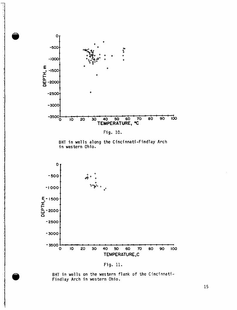
Ohio The most d i s t i n c t i v e feature of t he Ohio ground-water temperature map
(F ig. 9 ) i s the northward-trending high, along the C inc inna t i Arch i n the
western p a r t o f the s ta te . However, the geothermal-gradient map has a s l i g h t
negative c o r r e l a t i o n co inc iden t w i t h the arch. Because the l i t h o l o g y o f the
gen t l y d ipp ing Phanerozoic s t r a t a i s fa i r l y uni form throughout Ohio and west- e rn Pennsylvania, s h a l l ow subsurface v a r i a t i o n s i n the geothermal regime,
cannot r e a d i l y be a t t r i b u t e d t o l a t e r a l v a r i a t i o n s i n thermal conduc t i v i t y o f
the rocks. Moreover, t he reg iona l topography i s near ly f l a t . Therefore, the
h igher temperature o f the ground water co inc iden t w i t h the C inc inna t i Arch may r e s u l t from deeper convect ive ground-water movement along f a u l t s and v e r t i c a l
f rac tu res . A s i m i l a r h igh ground-water temperature anomaly i n southwestern Pennsylvania t rends southwestward through West V i r g i n i a and i n t o the southern-
most count ies o f Ohio. Cannon e t a l . (1980) proposed a conceptual model f o r a
convect ive system generating an anomaly i n shallow g l a c i a l formations. The
general p r i n c i p l e o f t he model may be app l ied as we l l t o two deep, conf ined aqui fers separated by a f rac tu red 1 i t h o l o g i c u n i t having aquiclude charac-
t e r i s t i c s , such as a shale o r marl. Convection through the f rac tu res would s h o r t - c i r c u i t between the two aqui fers . A we l l d r i l l e d d i r e c t l y above such a
convection c u r r e n t would have an anomalously h igh temperature gradient . A we l l d r i l l e d i n t o such a convection system away from a r i s i n g c u r r e n t would
have an anomalously low temperature gradient . An ana lys is o f the depth- temperature p r o f i l e s and depth-geothermal-gradient p r o f i l e s ca l cu la ted on the
bas is o f t he d i s t r i b u t i o n o f BHT throughout Ohio tends t o support the v a l i d i t y
of t he model. The depth-BHT diagram fo r w e l l s along the C inc inna t i Atch has a
wide s c a t t e r o f po in ts (F ig . 101, whereas s i m i l a r diagrams f o r areas eas t and
west of t he arch show ar rays o f p o i n t s along a f a i r l y cons is ten t slope (Figs. 11-15). Likewise, the depth-geothermal-gradient diagram f o r w e l l s along the
arch has a wide s c a t t e r o f the po in ts ,
p a r t i c u l a r l y i n the shal low zones (F ig. 161, whereas the same diagrams f o r t he
0
reg ions eas t and west o f t he arch show a f a i r l y cons is ten t geothermal g rad ien t
f o r most depths, w i t h i n the range from 15"C/km t o 30"C/km (Figs. 17-20). a 14
0
-5001
- 1 000
E r I- a w -2000. 0
-2 500-
- -1500*.
- 3000..
0-
-5008-
- I ooo*.
E-1500. .
I-
D
I"
; - 2000
- 2500
- 3000 -3500-
+ +
"r;t;t,++ + + +.,++q+ +
+ f+
( .
6.
: : : : : : : : : : : : : : : : : I
+ + +
+
* t + t
Fig . 10.
BHT i n w e l l s along the C inc innat i -F ind lay Arch i n western Ohio.
+ $+$2+ +
++
Fig . 11.
BHT i n w e l l s on the western f lank o f the C inc innat i - F ind lay Arch i n western Ohio.
15

+ 0-
- 500 -I 000
E-l 500
I-
a
e
r 4-2000
-2500
-3000
-3500.
+ A. ++
I .
,.
* -
'.
'.
*.
: : : : : : : : : : ; : : ; : ; : I
4 4b
+ &* +
01
-500..
- I O 0 0
- 1 500.. E - I
W Q
-2000..
- 2500
- 3000 ,.
++A+ + ++ + +
'
+ + $
++ +
Fig. 12 .
BHT in wells on the eastern flank o f the Cincinnati- Findlay Arch in central Ohio.
+ + E+ #,++ +
+ +* + + + t + $
+ +
+ +
+ +
Fig. 13.
BHT in wells in northeastern Ohio.
16

?# +* +*+ + + +++ +'.+ + ++ +
- 5 0 0
- IO00 E I l- a - - I S 0 0
g-2000
-2500
-3000
-3500'
.p ++ + + & + + +
++ + .
(.
+ '.
' +
'.
: : : " ' : : ' : ' ' : : '
0 -
-500
- I O 0 0
'- - I500 I t-
0 ti -2000
- 2 500
- 3000
-3500.
Fig. 14.
BHT i n wells i n eastern Ohio.
+ +
,' + + + +
*. *'*+$+
+ % ;
+ + ++ + + k +
'.
+ + -.
: : : : : f f : : : : : : : : 4
BHT i n wells i n southeastern Ohio.
17

0-
- 500..
- I ooo-* E < - I500** I- n g -2000..
-2500..
+ +
+*++;;+ ::>+++ +
+ ,+$p+* + + + + + ++ $ ++++#+ 4 + +
++ ++ + +
- I500 I tz g -2000,.
-2 500 * -
+
L
* *
+
- 3000
- 3500 0 io 20 30 40 50
dT/dZ ,T k m Fig. 16.
Geothermal gradient as a function of depth in wells along the Cincinnati- Findlay Arch in western Ohio.
+
+ + + + .K
++++?* + + +++ ; + +
++ + + + ++
+ + +
++ +
- 3000 I -3500
0 IO 20 30 40 50 60 d T / d Z ,OC/km
Fig. 17 .
Geothermal gradient as a function of depth in wells on the eastern flank of the Cincinnati-Findlay Arch in central Ohio.
18

0 -
-500
- 1000 E I !- a w -2000.. 0
-1500. .
-2500
- 3000
-3500 4
~ Fig. 18. I
Geothermal gradient as a function o f depth i n wells in northeastern Ohio.
*.
*+ +++ r +
* -
+ +y;+,+ + +
+ + +* + + +
+ '. +
+ ,.
+
I
+ +
-2500
-3000
-35001
+'i +++ ) . +
++ + + + ++* + $+
J.
* *
*.
4
+ + + ++ 1 * + +
+
+ +
+
Geothermal gradient as a function of depth in wells in eastern Ohio. 19

-r, + I - + + +
+ + + + + ++ +
+
+
. . 4
0 IO 20 30 40 50 60 -35001
d T / d Z , O C / km Fig. 20.
Geothermal gradient as a function of depth i n wells i n southeastern Ohio.
Therefore, t e r r e s t r i a l heat w i t h i n the sedimentary cover along the Cincinnati Arch may be t ransferred both by convection and by conduction; i n cont ras t , the uniformity of the geothermal gradient e a s t and west of the arch suggests predominantly conductive heat t ransfer . Accordingly, e f f o r t s t o f i n d deep holes fo r heat-flow measurements were concentrated i n eastern Ohio. One su i tab le well was measured i n Washington County (F igs . 21, 22, and App. C ) , and another i n Sumnit County ( F i g s . 23, 24, and App. D ) .
Pennsylvania The most prominent feature on the geothermal-gradient map of
Pennsylvania (F ig . 7) is the northeast-trending anomaly centered on Venango County i n the northwestern par t of the s t a t e . The anomaly maximum exceeds 30"C/km, whereas the gradient for the remainder of Pennsylvania ra re ly exceeds 25"C/km (Figs . 25-32). An exception is a weak h i g h defined by the 30"C/km contour a t the common corners of Jefferson, Clearf ie ld , and E l k Counties eas t - southeast of the Venango anomaly (Fig . 7). Gradient surveys were made i n the Morrison well (Fig. 33) i n Venango County and i n the Bowser well (F ig . 34) i n
20

I I + NOBLE
K + MORGAN
WASHINGTON
0 l O k m - SCALE
0 HEAT FLOW SITE A WELL 3236 + CORE/CONDUCTIVlfY S I T E E WELL 2386 I WELL 2177 F WELL 2181 J WELL 2178
H WELL 2176 G WELL 2387 a WELL 2180
0-
-50..
- 100..
- 150-
-200..
E -250..
-300..
- 350-
-400**
-450.8
-500s.
- 550,
-6004
i W 0
.
4 5 IO 15 20 25 30 0
+ + + + + + + + + + + + + + + + + + + + + + + + + + + + + + + + + + + + +
F i g . 21.
Wells i n Morgan, Noble, and Washington Counties, Ohio a t which heat-flow measurements were made or core was col- lected for thermal conductiv- i ty determi na ti ons .
F i g . 22.
Depth/temperature prof i le i n Well 3236 i n Washington County, Ohio.
21

c
+ COREKONDUCTIVITY SITE
0 HEAT PRODUCTION SAMPLE SITE -100
3,40 4-M
+ '
Fig. 23. >
Depth/temperature profile in Barberton well in Summit County, Ohio. -700 3
+ + + + + + +
+ + + + +
+ +
+ + + + +
- ::::/ I O 0 0 0 IO 20 30
TEMPERATURE ,Y
22

0-
- I O 0 0
-2000
'- - 3000 I I- Q
-4000
- 5000
* +
( '
* *
',
+ + +
-2000
E
c- Q
- -3000 r
n -4000
-5000 * I
-6000 ('
-70004
f - 6000
- 7000 0 20 40 60 80 100 120 140
TEMPERATURE, "C Fig. 25.
++ # '
+ ++<+*+$$$+>+ * ++
+ * '
+ ''
: : : : : : : : : : : I
BHT in wells in northwestern Pennsylvania.
- 1000 f 2&++ +
Fig. 26.
BHT in wells in southwestern Pennsylvania.
23

E I t a W Q
- IOOO-.
-2000,-
-3000..
-4000..
-5000,.
-6000..
+ ++* + + +
+ +
+
+
* loo 120 140 20 40 60 80 - 70000
TEMPERATURE , O C
Fig. 27.
BHT in wells in north-central Pennsylvania.
- 1000 3 ++++ + +>+ ++
"**. A +
+ +++* + ++ + ##A++:+ * ++ + + * *
+ + +
+ - 7000 I
TEMPERATURE, O C
100 120 140 0 20 40 60 80
Fig. 28.
BHT in wells in central and northeastern Pennsylvania.
24

0-
- 1 000
-2000
E. -3000 I t- a
-4000
+ ++ + + +
*.
+
+ +
-2000
E f -3000 t- 0 W p - 4000
- 5000
-6000
- 7000
- 5000
-6000
+t + ++ +
*. +ft'++++@:* $%e +
+ + + +
+ +
- -
a .
t
-7000 4 4
0 IO 20 30 40 50 60
dT/dZ,OC / km
Fig. 29.
Geothermal gradient as a function o f depth i n wells in northwestern Pennsylvania.
+ + + +
+ # +**+ *2*2 *+ + + + + *+++$*++ - IO00 t + +
Geothermal gradient as a function of depth in wells in southwestern Pennsyl van ia .
25
0
- 1000
- 2000
E -3000
0-
- 1000..
- 2000 E - -3000%. I I- a -4000.-
-5000.-
-6000,.
-7000
.I
r I- $ -4000 0
( *
+ - I
- 5000
-6000
+ + + ++ ++ ++ ++ 3 + **+
++* ++ '@+ +
+
+ +e$+: :+ # + +
+
+
7000 1 I 0 IO 20 30 40 50 60
dT/d Z,OC / km
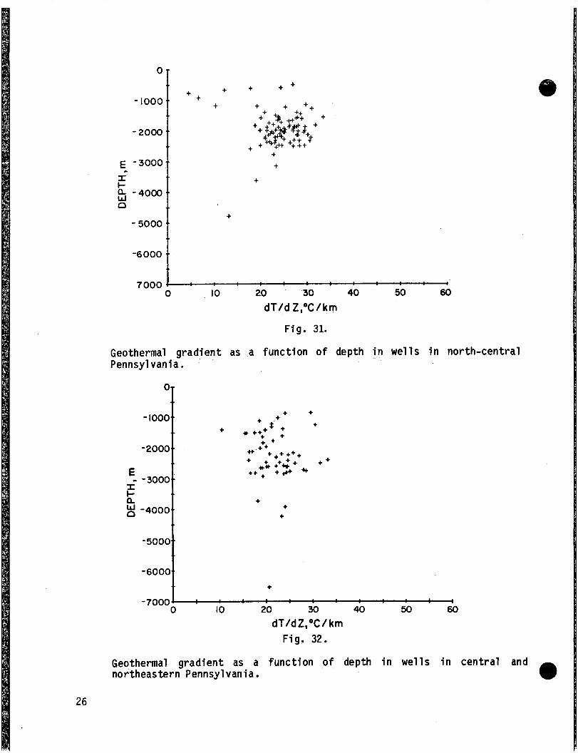
F i g . 31.
Geothermal grad ient as a funct ion o f depth i n w e l l s i n north-centra l Pennsylvania .
+ + +
+ $ ' +
+ 0 ++,* +
+
+!+ + *' +,++++ + *%;+ct+* + + + +#+
+ + +
+ +
0 Geothermal grad ient as a funct ion o f depth i n w e l l s i n c e n t r a l and northeastern Pennsylvania.
26

* (1.5 HFU 1 (1.3 HFU)
A
20 0
210023 220
OC(2.0 HFU)
0 D(1.8 HFU)
~ ( 1 . 3 HFU)
A(1.2 HFU)
I 0 NEW HEAT FLOW WELL C MORRISON D BOWSER
A PUBLISHED HEAT FLOW WELL 0 HEAT PRODUCTION SAMPLE S I T E
50 IOOkm 0 - SCALE
F i g . 33.
Wells and outcrops i n Pennsylvania a t which heat-flow measurements were made or samples were col lected fo r heat-production determinations.
Clarion County. In a d d i t i o n , core samples from the Bowser well and samples from several wells near the Morrison well were used for measurement of thermal conductivit ies.
The Morrison well had been d r i l l e d to 323.1 m nine months before mea- surements were made. T h e Bowser well caved a t 458 in i n 1969 and i s currently
producing a small amount o f gas from Mississippian sandstones i n the uppermost 243 m. Because of gas production, ground-water disturbances and, poor l i t h o - logic control , only measurements between depths of 243 m and 353 m were considered re1 iable. Depth/temperature prof i les for the two wells a re plotted i n F i g s . 35 and 36. Basic temperature data and the relevant corrections are included i n Apps. E and F. Linear regression of the depth/temperature points w i t h i n the useful in te rva ls i n the Morrison and Bowser wells yields mean uncorrected gradients of 22.63"C/km and 22.53"C/km respectively, and a correlat ion coef f ic ien t of 0.99. Extrapolation of these gradients t o a depth of 30.5 m gives values of 6;30°C and 7.36"C. These values d i f f e r because of differences i n the measured temperatures a t depth. They are considerably
27
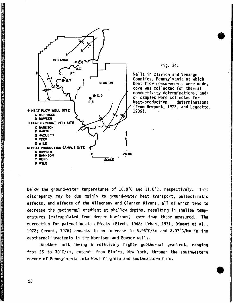
Fig. 34.
Wells i n Clarion and Venango Counties, Pennsylvania a t which heat-flow measurements were made, core was collected for thermal
' conductivity determinations, and/ or samples were col lected for heat-produc t ion de termi nations
/ (from Newport, 1973, and Leggette, 1936). 0 HEAT FLOW WELL SITE
C MORRISON D BOWSER
0 BANKSON P MARSH 0 HAZLETT R REED S WILE
5 BOWSER 6 BANKSON 7 REED 8 WILE
+ COREKONDUCTIVITY SITE
0 HEAT PRODUCTION SAMPLE SITE
0 25 km
SCALE
below the ground-water temperatures of 10.8"C and l l . O ° C , respectively. T h i s discrepancy may be due mainly t o ground-water heat transport, paleoclimatic effects, and effects of the Allegheny and Clarion Rivers, all of w h i c h tend t o decrease the geothermal gradient a t shallow depths , resulting i n shallow temp- eratures (extrapolated from deeper horizons) 1 ower t h a n those measured. The correction for paleoclimatic effects (Birch, 1948; Urban, 1971; Diment e t a1 ., 1972; Cermak, 1976) amounts t o an increase t o 6.96"C/km and 3.07"C/km i n the geothermal -gradients i n the Morrison and Bowser wells.
Another be l t having a relatively higher geothermal gradient, ranging from 25 t o 30"C/km, extends from Elmira, New York, through the southwestern corner of Pennsylvania i n t o West Virginia and southeastern Ohio .
28

+ + + + + + + + + + + + + + + + + + + + + + + + + + + + + + $
0 -
-90..
-100..
-150..
E-200..
f -250..
W 0
-300..
-350.
-400..
-450
-5006
'
8
5 IO 15 20 25
Fig. 36.
Depth/temperature p r o f i l e i n Bowser we l l i n C l a r i o n County, Pennsylvania.
Fig. 35.
Depth/temperature p r o f i l e i n Morrison w e l l i n Venango County, Pennsylvania.
+
-900' I 0 5 IO 15 20 25
TE M PER ATU R E, OC
29

Thermal Conductivity I n practice terrestrial heat flow, q i s approximated by
- q = K ( A T ~ A Z ) ,
where AT i s the temperature difference over a f i n i t e depth interval AZ com- prised of material having a mean thermal conductivity of K.
Thermal conductivity of the rock formations was determined by measure- ments on core samples using the divided-bar technique (Birch, 1950). The measurements were obta ined on machined core-discs, 1.27 t o 3.18 cm thick, under an axial pressure of 50 bars t h a t reduced contact resistance t o negligible values. Temperatures across the d iv ided bar were measured w i t h thermistors calibrated t o - + 0.02OC w i t h a platinum resistance thermometer. Each core sample was measured for thermal conductivity first "off-the-she1 f " and second after saturation w i t h water i n a vacuum chamber.
A t o t a l of 77 core samples were obtained from wells i n Washington, Noble, and Morgan counties i n southeastern Ohio (App. G), 29 core samples were taken from the Barberton well (App. H ) , and 37 other core samples were ob- tained from wells i n southern, central, and northern Ohio (App. I ) . A total of 64 core samples were taken from wells i n Venango and Clarion counties i n Pennsyl van ia ( App . J 1.
Computations of the terrestrial heat flow were done using the interval method. Each well was divided in to a series of uniform depth intervals ( A Z ) .
The temperature difference ( A T ) fo r each interval was measured and the mean thermal conductivity (K) was computed. The measured thermal conductivities of representative core samples of each rock u n i t penetrated were averaged t o determine the mean thermal conductivity for each rock type. These means were averaged by weighting the percentage of each lithologic type comprising each depth interval ( A Z ) i n wells from which no core samples were available. The mean heat flow of the evaluated intervals i s considered t o be the best approx- imation for the observed terrestrial heat flow. The calculated heat-flow values, w i t h appropriate corrections f o r each s i te , are given i n Table 11.
Three basement samples from O h i o and five from Pennsylvania were analyzed for U(ordinary), 232Th, and K20 by the Los Alamos National Laboratory. Five samples of shale from Ohio and 11 samples from Pennsylvania also were analyzed a t the Los Alamos National Laboratory for U(ordinary) 232Th and K. Analysis of U(ordinary), 232Th, and Ra contents i n 34
30
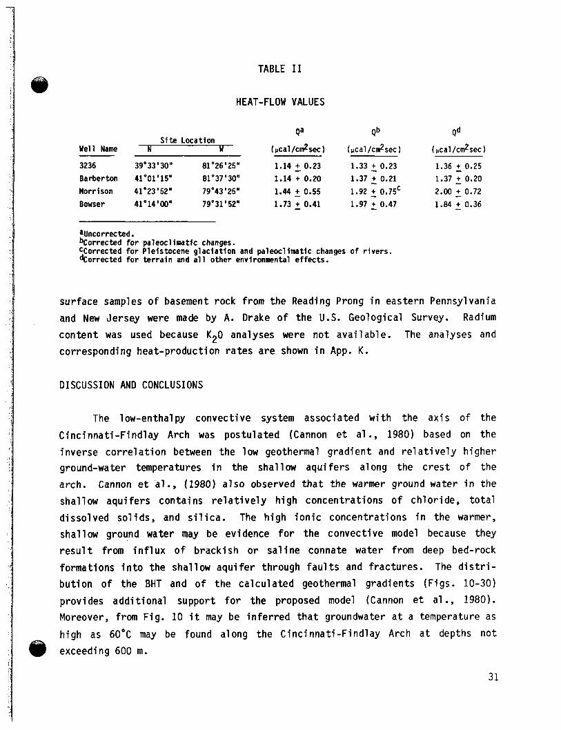
TABLE I 1
HEAT-FLOW VALUES
Qa Qb Qd
1.33 - + 0.23 - 1.37 - + 0.21 -
41'23'52" 79'43 '25" 1.44 - + 0.55 1.92 - + 0.75' - 1.97 - + 0.47 -
Site Location w (vcal/c&sec) (kcal/cm2sec) (,,tal /cm2sec
1.36 + 0.25
2.00 + 0.72 1.84 + 0.36
39'33 '30" 81 '26 '25' 1.14 - + 0.23 41'01 '15'' 81'37 '30' 1.14 + 0.20 1.37 + 0.20
41 '14'OO" 79'31'52" 1.73 - + 0.41
Well Name
3236 Barberton Morrison Bowser
auncorrected. bCorrected for paleocl imatic changes. CCorrected for Pleistocene glaciation and paleocl imatic changes o f rivers. korrected for terrain and al l other environmental effects.
sur face samples o f basement rock from the Reading Prong i n eastern Pennsylvania
and New Jersey were made by A. Drake o f t he U.S. Geological Survey. Radium
conten t was used because K20 analyses were n o t ava i lab le . The analyses and corresponding heat-production r a t e s are shown i n App. K.
DISCUSSION AND CONCLUSIONS
The low-enthalpy convect ive system associated w i t h the a x i s o f the
C inc innat i -F ind lay Arch was pos tu la ted (Cannon e t a1 ., 1980) based on the
inverse c o r r e l a t i o n between the low geothermal g rad ien t and re1 a t i v e l y h igher ground-water temperatures i n the shal low aqu i fe rs along the c r e s t o f the
arch. Cannon e t al., (1980) a l s o observed t h a t the warmer ground water i n the
shal low aqu i fe rs conta ins r e l a t i v e l y h igh concentrat ions o f ch lo r ide , t o t a l
d isso lved so l i ds , and s i l i c a . The h i g h i o n i c concentrat ions i n the warmer,
shal low ground water may be evidence f o r the convect ive model because they
r e s u l t from i n f l u x o f b rack ish o r s a l i n e connate water from deep bed-rock
formations i n t o the shal low a q u i f e r through f a u l t s and f rac tu res . The d i s t r i -
bu t i on o f t he BHT and o f t h e ca l cu la ted geothermal gradients (Figs. 10-30)
provides add i t i ona l support f o r the proposed model (Cannon e t a1 ., 1980). Moreover, from Fig. 10 i t may be i n f e r r e d t h a t groundwater a t a temperature as
h igh as 60°C may be found along the C inc innat i -F ind lay Arch a t depths n o t exceeding 600 m.
31

The uncorrected heat flow i n C la r ion County, Pennsylvania i s h igher than
average f o r the eastern Un i ted States (Diment e t a1 ., 1972; Sass e t a1 ., 1976). When cor rec ted fo r environmental cond i t ions , t he heat f lows i n C la r ion and
Venango count ies a re markedly h igher than the mean o f 1.34 heat- f low u n i t s
(HFU) f o r the eastern Uni ted States (Urban, 1971). The values de f ine a l o c a l heat- f low h igh n o t associated w i t h o ther repor ted heat- f low highs i n New York
(Urban, 1971; Hodge, D. S., 1979, personal communication) nor i n o ther nor th-
eastern s ta tes (Sass e t al., 1980). The pronounced nor theas t - t rend ing trough (F ig. 9 ) on the ground-water
temperature map o f Pennsylvania and the decreasing hydrau l i c g rad ien t i n
northwestern Pennsylvania may r e s u l t from c o l d recharge a long the Allegheny
Mountains and the Allegheny drainage basin, respec t ive ly . I f so, the
geothermal-gradient highs (F ig . 7) mark areas o f h igher than average con-
duc t ive heat f low. The area o f e levated ground-water temperature (Fig. 9) i n
southwestern Pennsylvania corresponds roughly w i t h above-average geothermal g rad ien ts (F ig . 6) .
The Bouguer g r a v i t y map o f Pennsylvania i nd i ca tes a southwest-trending
g r a v i t y l o w centered a t P i t t sbu rgh (F ig. 4). The wavelength o f southwest-
t rend ing aeromagnetic h igh centered i n Venango County (U. S. Geological
Survey, 1979) may i n d i c a t e t h a t the source o f t he anomaly i s w i t h i n the upper
c r u s t . B i r c h e t al., (19681, Roy e t al., (19681, and Lachenbruch (1968, 1970)
observed a l i n e a r r e l a t i o n between heat f l o w (0) and rad iogenic heat produc-
t i o n (A): Q = a + b A ,
where a i s t he p o r t i o n o f t he observed heat f l ow o r i g i n a t i n g from the lower
c r u s t and mantle. The c o e f f i c i e n t corresponding t o the thickness o f t he
heat-producing l a y e r o f t h e upper c r u s t i s b. The values o f a and b a re 0.69 and 6.9 respec t i ve l y f o r t he eastern heat- f low province, according t o Costa in
e t al., (1980). For t h e topograph ica l l y cor rec ted heat f lows o f Venango and C l a r i o n counties, t he r e l a t i o n would i n d i c a t e upper c r u s t a l heat product ions
o f 11.59 heat-generation u n i t s (HGU) and 13.48 HGU respec t ive ly , which a re much h igher values than heat product ion from the Precambrian basement deter-
mined i n nearby E r i e County (App. K ) .
32

Based on a two-layer model, t h a t crustal thickness is approximately 36-45 km (Pakiser and Steinhart , 1964). Assuming a mantle heat flow of 0.4 HFU (Roy e t a l . , 1968) and a lower crustal contribution of 0.95 HFU (Urban, 19711, the upper crustal contribution would be 1.05 HFU for Venango County and 0.89 HFU f o r Clarion County. T h i s is approximately three times the typical upper crustal contribution fo r the eastern heat-flow province. Perhaps some excess heat flow is due t o the highly radiogenic Pennsylvanian and Mississip- pian shales (App. K ) , b u t the heat production of the shales beneath the Venango anomaly differs 1 i t t l e from t h a t of samples bel ow non-anomal ous areas i n Ohio. Moreover, the Venango anomaly does not coincide w i t h the center of the Appalachian Basin, where the sedimentary cover is thickest ( F i g . 1) . Therefore, the anomaly may be associated w i t h abnormally h i g h heat production i n the upper c rus t . A more detai led gravimetric survey might provide more information on the nature of the anomaly. I f the anomaly is associated w i t h a younger, fel s i c intrusion, characterized by a h i g h concentration of radiogenic elements, such a survey would he lp delimit the spa t ia l d i s t r ibu t ion of the anomaly.
The heat-flow values found el sewhere a re we1 1 w i t h i n the commonly expected values cha rac t e r i s t i c of the Allegheny Plateau, (1.22 t o 1.89 HFU) (Joyner, 1960).
SUMARY AND RECOMENDATIONS
Two types of geothermal anomalies were encountered d u r i n g the course of the project. The anomaly i n western Ohio is of a convective character, limited t o moderate depths w i t h i n the sedimentary cover. Ground water, a t temperatures t h a t may be useful i n local agr icul tural and space-heating projects , seems t o convect from deeper formations t o shallow zones through the system of f a u l t s and f rac tures associated w i t h the Cincinnati-Findlay Arch. Further research e f f o r t s emphasize detai led mapping of the f a u l t and f rac ture system along the arch and fuller character izat ion of the hydrothermal phenomena associated w i t h the system. Side-looking airborne radar combined w i t h infrared photography would be useful i n mapping the f a u l t s and f rac tures associated w i t h the arch. Ground water should be sampled and analyzed from a l l avai lable wells.
The heat-flow anomaly i n northwestern Pennsylvania seems to be associ- a ted w i t h an anomalous heat source w i t h i n the upper c rus t . The source
33

probably i s within the Precambrian basement, and may be a felsic intrusion having a relatively high concentration of radioactive elements. To determine the validity of this interpretation, a detailed gravimetric survey of the anomalous region and additional heat-fl ow measurements are recommended. The l a t t e r should be determined on a t least f ive cores from wells 500-1000 m deep. Additional heat-flow measurements are recommended in other areas of Pennsylvania where geothermal gradients exceed 30"C/km (Fig. 6).
ACKNOWLEDGMENTS
The assistance of M. W. Schlorholtz, G. G. Maurath, M. F. Schmidt, and M. S . Cannon while graduate students a t Kent State University is gratefully acknowledged.
REFERENCES
American Association of Petroleum Geologists and U.S. Geological Survey, 1976,
Barbis, F. C . , 1978, Rb-Sr geochronology of the Precambrian basement of Ohio,
Subsurface temperature map of North America.
O h i o S t a t e Univ. unpub. M.S. thesis, 83 p.
Bass, M. N . , 1960, Grenville boundary i n Ohio, J. Geol., v. 68, p. 673-677.
rch, F., 1948, The effects of Pleistocene climatic variations upon geothermal gradients, Am. J . Sci ., v. 246, p. 729-760.
rch, F., 1950, Flow of heat i n the Front Range, Colorado, Geol. SOC. Am. B u l l . , V . 61, p. 567-630.
rch, F., Roy, R. F., and Decker, E. R., 1968, Heat flow and thermal history in New England and New York, in Zen E. , White, W. S . , Hadley, J . B., and Thompson, J. B., Jr . , ed., Studies of Appalachian Geology: Northern and Maritime, p. 437-451, Interscience, New York.
llinger, G. A. , 1973, Seismicity and crustal uplift i n the southeastern United States, Am. J . Sci. , v. 273A, p. 396-408.
Bradley, E. A. , and Bennett, T. J . , 1965, Earthquake history o f O h i o , Seismol. SOC. Am. Bull., V . 55, p. 745-752.
Cannon, M. S . , Tabet, C. A., and Eckstein, Y . , 1980, A low enthalpy convective system i n western Ohio, Geotherm. Resour. Coun. Trans., v. 4, p. 105-108.
34

Cermak, V . , 1976, Paleoclimatic effect on the underground temperature and some problems o f correcting heat flow, i n Adam, A., ed., Geoelectric and geothermal studies, east-central EuropeTSoviet Asia, p. 56-66, Akad. Kiado, Budapest.
Collins, H . R., 1979, Ohio i n The Mississippian and Pennsylvanian (Carbonif- erous) Systems i n the U n i t 3 States, U. S. Geol. Surv. Prof. Paper 1110-E, p . El-E26.
Costain, J . K . , Glover, L. , and Sinha, A. K., 1980, Low-temperature geothermal resources i n the eastern United States, EOS, v. 61, p. 1-3.
Diment, W. H., Urban, T. C . , and Revetta, F. A. , 1972, Some geophysical anom- alies i n the eastern United States, i n Robertson, E. C. , ed., The Nature of the Sol id Earth, McGraw Hi1 1 , p. 544-R4.
Duecker, J . C. , 1954, Gravity traverse i n northeastern Pennsylvania, Am. Geophys. Union Trans., v . 35, p. 503-507.
Gonterman, J. R., 1973, Petrographic study of the Precambrian basement rocks of Ohio , Ohio State Univ . unpub. M.S. thesis, 139 p.
Gray, C. , and Shepps, V. C. , 1960, Geologic map of Pennsylvania, Pennsylvania Geol . Surv.
Green, D. A., 1957, Trenton structure i n Ohio, Ind iana , and northern Illinois, Am. Assoc. Petroleum Geologists B u l l . , v . 41, p. 627-642.
Haidarian, M. R., 1976, Geophysical investigation of a gravity minima i n northwestern O h i o , Bowling Green State Univ. unpub. M.S. thesis, 56 p.
Heiskanen, W. A. and Uotila, U. A., 1956, Gravity survey of the state of O h i o , O h i o Geol. Surv., Rept. Inv. 30.
Hofmann, C . M., Faure, G., and Janssens, A., 1972, Age determination of a granite gneiss from t h e Precambrian basement o f Scio to County, O h i o , O h i o J . Sci., v. 72, p. 49-53.
Joyner, W. B., 1960, Heat flow i n Pennsylvania and West Vi rg in i a , Geophysics, V. 25, p. 1229-1241.
Kane, M. F., 1961, Structure of p lu tons from gravity measurements, U.S. Geol. Surv. Prof. Paper 424-C, p. C258-CZ59.
Kappelmeyer, 0. and Haenel, R. , 1974, Geothermics w i t h special reference t o application, Geoexploration Monographs, ser. 1 , no. 4 , Gebruder Borntraeger, Berlin.
Lachenbruch, A. H., 1968, Preliminary geotherma7 model for the Sierra Nevada, J . Geophys. Res., v. 73, p. 6977-6989.
, 1970, Crustal temperature and heat production: imp1 ications of the linear heat flow relation, J . Geophys. Res., v. 75, p. 3291-3300.
35

Lapham, D. M., 1975, I n t e r p r e t a t i o n of K-Ar and Rb-Sr i s o t o p i c da t e s from a Precambrian basement core, Erie County, Pennsylvania, Pennsylvania Geol . Surv. In f . Circ. 79, p. 26.
Legget te , R. M., 1936, Ground water i n northwestern Pennsylvania, Pennsylvania Topog. and Geol. Surv. B u l l . W-3, 215 p.
Lidiak , E. G . , Marvin, R. F., Thomas, H. H . , and Bass, M. N., 1966, Geochron- ology of the mid-cont inent reg ion , United S t a t e s , 4. Eastern area, J . Geophys. Res., v. 71, p. 5427-5438.
McCormick, G. R . , 1961, Petrology of Precambrian rocks of O h i o , Ohio Geol. Surv. Rept. Inv. 41, 60 p.
Mongel l i , F., 1970, Inf luence of rivers on geotemperatures , Annali d i Geo- f i s i c a , v . 23, p. 205-212.
Newhart, J . A., 1975, Gravi ty and magnetic geophysical i n v e s t i g a t i o n s of Sandusky, Seneca, and po r t ions of Hancock and Wood Counties , O h i o , Bowling Green S t a t e Univ., unpub. M.S. thesis, 75 p.
Newport, T. C. , 1973, Summary ground-water resources o f Clarion County, Pennsylvania , Pennsylvania Topog. and Geol. Surv., Water Resour. Rept. 32, 42 p.
Owens, G. L . , 1967, The Precambrian surface of Ohio, Ohio Geol. Surv. Rept. Inv. 64, 9 p.
Pakiser, L. C., and S t e i n h a r t , J . S., 1964, Explosion seismology i n the western hemisphere, i n Odishaw, H. , ed., Research i n Geophysics, p. 123-147, MIT Press, CambridgeFMass.
Pincus, H. J . , 1960, Geological i n t e r p r e t a t i o n of major O h i o g r a v i t y anomalies ( a b s . ) , J . Geophys. Res., v. 65, p. 2517.
Q u i c k , R. C. , 1976, Gravity-magnetic survey of p o r t i o n s o f Wood and Lucas Counties , O h i o , Bowling Green S t a t e Univ. unpub. M.S. thesis, 81 p.
Ross, M. E . , 1972, Precambrian qua r t zo - fe ldspa th i c gne i s s from the Herman 1 A well, Erie County, Ohio, O h i o 3. Sc i . , v. 72, p. 105-109.
Roy, R. F., Decker, E. R. , Blackwell, 0. D. , and Birch, F., 1968, Heat flow i n the United S t a t e s , J . Geophys. Res., v. 73, p. 5207-5222.
Rudman, A. J . , Summerson, C. H . , and Hinze, W. J . , 1965, Geology of basement i n midwestern United S t a t e s , Am. Assoc. Petroleum Geologis t s B u l l . , v. 49, p. 894-904.
Sass , J . H. , Blackwell, D. D. . , Chapman, D. S., Costain, J. K., Decker, E. R . , Lawver, L. A., and Swanberg, C . A. , 1980, Heat flow from the crust of the United S t a t e s , i n Touloukian, Y. S., Judd, W. R., and Roy R. F., eds. , Physical P r o p e r t x s of Rocks and Minerals, McGraw-Hill, p. 503-548.
36

Sass, J . H . , Diment, W. H . , Lachenbruch, A. H . , Marshall, B. V . , Munroe, R. J. , Moses, T. H., J r . , and Urban, T. C. , 1976, A heat-flow contour map of the conterminous United States , U.S. Geol. Surv. Open-File Rept. 76-756, 24 p.
Saylor, T. E . , 1968, The Precambrian i n the subsurface of northwestern Pennsylvania and adjoining areas, Pennsylvania Geol. Surv. Inf. Circ. 62, 25 p.
Schlorhol t z , M. , 1979, Terrestr ia l heat flow i n southeastern Ohio, Kent State Univ. unpub. M.S. thesis, 77 p.
Scotford, D. M., 1964, Cincinnati Arch: mineralogical-statistical evidence of post-Ordovician or igin, Am. Assoc. Petroleum Geologists Bull., v . 48, p. 427-436.
Shearrow, G. G . , 1957, Geologic cross section of the Paleozoic rocks from northwestern t o southeastern Ohio, Ohio Geol. Surv. Rept. Inv. 33, 42 p.
Spa11 , H. , 1979, Understanding seismicity w i t h i n the continents, Earthquake Inf. Bull., v . 11, p. 80-88.
Summerson, C. H. , 1962, Precambrian i n Ohio and adjoining areas, Ohio Geol. Survey Rept. Inv. 44, 16 p.
U . S. Geological Survey, 1979, Aeromagnetic map o f Pennsyl vania, Map GP-924, 1:500 000.
Urban T., 1971, Terrestr ia l heat flow i n the Middle Atlantic States , Un iv . Rochester, unpub. Ph.D. dissert., 398 p.
Wallace, R. L. , 1978, Gravity survey o f the Kent quadrangle, Portage County, O h i o , Kent S ta t e Univ. , unpub. M.S. thesis, 132 p.
Water Well Journal, 1979, Heat pump update, v. 33, no. 10, p. 50, and unpub . materials on f i l e a t National Water Well Association, Worthington, Ohio.
Willard, B., 1962, Pennsylvania geology summarized, Educational Series, v . 4 , p. 17.
Williams, D. W., 1976, The Anna, Ohio, earthquake zone and the establishment of the Anna gravity network, Univ. Michigan, unpub. M.S. thesis, 73 p.
Woollard, G. P., 1958, Areas of tectonic a c t i v i t y i n the United States as indicated by earthquake epicenters, Am. Geophys. Union Trans., v. 39, p. 1135-1150.
Woollard, G. P., 1972, Regional var ia t ions i n gravity, i n Robertson, E. C . , ed., The Nature of the Solid Earth, McGraw Hill, p. 4 6 3 - m .
Woollard, G. P., and Joesting, H. R. , 1964, Bouguer gravity anomaly map o f the United States (exclusive of Alaska and Hawaii), Am. Geophys. Union and U.S. Geol . Surv.
37
York, J . E., and Ol iver , J . E., 1976, Cretaceous and Cenozoic f a u l t i n g i n eastern Nor th America, Geol. S O C . Am. Bu l l . , v . 87, p. 1105-1114.

APPENDIX A
BOTTOM-HOLE TEMPERATURES I N O I L AND GAS WELLS
I N OHIO
39

County
Adarns A1 l e n
Ash1 and
Ash tabu1 a
Athens
BHT ("C)
29.40 23.89 22.22 35.56 30.56 30.56 33.89 36.67 20.59 43.89 27.78 32.22 32.22 32.78 39.44 32.22 34.44 23.33 32.78 34.44 50.56 '32.22 32.22 32.22 45.00 37.78 32.78 42.02 22.78 31.67 23.33 29.44 25.56 34.44
14.17 13 -83 13.58 13.58 13.25 12.58 12.58 12.63 12 -61 12.67 11.23 10.96 10.96 11.02 11.06 11.01 11.06 11.07 11.03 11.02 10.83 11.08 10.98 11.33 11.08 11.32 13.56 13.72 14.03 13.22 13.56 13.55 13.99 13.22
Depth (m)
1167.8 619.15 608.8 955.6 995.8 864.41 928.18 1473.71 242.93 1353.62 1123.49 969.57 959.82 1075.33 1246.63 904.34 1018.34 1221.64 954.02 1167.38 1962.91 1085.09 1021.69 1129.59 1889.76 1143.61 1112.52 1481.33 508.10 1054.61 429.16 538 58 513.59 1223.16
dT/dz
13.40 17.10 14.94 24.10 17.93 21.92 24.49 17.16 37.40 24.26 15.64 22.64 22.88 20.83 23.34 24.27 23.68 10.30 23.55 20.60 20.56 20.04 21.43 19.01 18.24 23.78 17.76 19.64 18.31 18.01 24.53 31.28 23.94 17.79
40

County
Augl a i ze
But1 e r
C a r r o l l
Champaign
Clarke C1 i nton
C o l umb i ana
Cos hoc ton
BHT ( " C )
26.67 23.89 32.78 28.30 30.0 41.11 47.22 47.22 18.33 40.56 45 .O 43.33 46.11 28.33 27.78 26.11 23.9 33.9 25.6 67.50 44.44 71.11 41.67 96.11
65.56 45.56
30 . 56 46.67 42.78 37 -22
49.44 39.44
14.0 13.28 13.47 14.61 14.5 11.66 11.45 11.53 11.67 11 -72 11.75 11.81 11.67 13.6 14.28 14.53 13.8 13 . 13.7 11.31 11.12 11.38 11.61 11.39
11.39 11.61
12.34 12.31 12.29 12.25
12.21 122.38
Depth
(m)
521.6 541.7 935.4 895.2
1004.62 1687.07 1880.01 1881.84 373.38
1713.89 1734.31 1680.97 1891.28 686.3 815.3
1111.61 993.4
1019.3 1054.7 2701.14 1804.42 3179.67 1625.19 3134.87
1904.70 1661.77
1056.13 1905.91 1351.18 1234.74
2042.16 1232 .O
dT/dz
25.8 37.8 21.3 13.30 16.53 17.78 19.34 19.28 19.43 17.13 19.51 19.10 18.51 21.40 17.20 13.71 10.5 20.3 11.6 22.05 19.54 20.11 20.01 29.07
28.60 21.65
18.36 19.07 23.73 21.35
19.25 23.18
41

County
Craw f o r d
Defiance
Del aware
E r i e
F a i r f i e l d
Fayet te Frank1 i n
Ful ton
42
BHT
("C) 33.33 34.44 31 .ll 23.89 22.22 35.56 30.56 38.89 23.89 24.44 40.0 32.8 29.4 40.0 29.4 31.1 28.3 25.6 29.4 34.4 25.6 33.3 33.33 24.44 26.11 24.44 33.33 24.44 42.2 32.8 35.5 31.1 28.3
Tgw ("C) 12.39 12.40 12.49 13.83 13.58 13.58 13.25 12.8 2.7 12.83 12.89 12.92 12.5 13.0 12.97 12.89 13.08 13.11 12.89 12.5 12.69 12.75 13.11 12.87 12.84 12.89 13.09 12.88 13.56 13.11 13.17 13.2 12.42
Depth
(m) 994.56 1045 16 1008.58 619.15 608.8 955.6 995.8 1101.1 569.1 569.7 1033.6 1030.6 946.7 862.5 1224.3 1059.6 710.3 702.4 1132.8 1182.8 555.1 1193.8 1139.95 736.09 837.9 725.42 1149.71 691.29 1435 .O 1104.7 827.8 1144.7 896.4
dT/dz
22.42 22.4 19.67 17.1 14.94 24.1 17.93 23.7 20.75 20.4 27 .O 19.9 18.4 32.4 13.8 17.7 22.4 18.6 15 .O 19.0 24.8 27.55 18.83 16.75 16.75 16.98 18.68 17.87 20.4 18.3 28.0 16.1 18.3
County
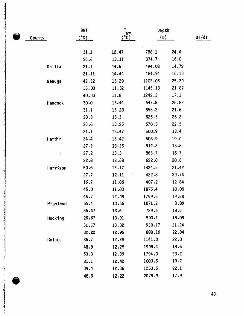
Gal 1 i a
Geauga
Hancock
Hardi n
Harrison
Highland
Hocking
Holmes
BHT ("C)
31.1 26.6 21.1 21.11 42.22 35.00 40.00 30.0 31.1 28.3 25.6 21.1 24.4 27.2 27.2 22.8 50.6 27.7 16.7 45.0 46.7 56.4 56.47 26.67 31.67 32.22 36.7 48.9 53.3 31.1 39.4 48.9
12.47 13 . 11 14.5 14.44 13.29 11.32 11.8 13.44 13.28 13.3 13.25 13.47 13.42 13.25 13.3 13.58 12.17 12.11 11.86 11.83 12.08 13.56 13.6 13.01 13.02 12.96 12.28 12.28 12.39 12.42 12.36 12.22
788.1 874.7 494.08 484.94 1203.05 1145.13 1242.3 647.8 855.2 625.5 578.3 600.9 606.9 912.2 863.7 622.8 1824.5 422.8 407.2 1875.4 1799.5 1071.2 729.6 800.1 938.17 888.19 1141 .O 1998.4 1794.0 1003.5 1253.5 2078.9
24.6 16.0 14.72 15.13 25.39 21.87 17.1 26.82 21.6 25.2 22.5 13.4 19 .o 15.8 16.7 28.6 21.42 39.74 12.84 18.00 19.58 8.89 18.6 18.09 21.24 22.84 22 .o 18.6 23.2 19.2 22.1 17.9
43

County
Huron
Jackson
Jef ferson
K nox
Lawrence
L i c k i n g
BHT
("C)
32.22 32.22 33.9 21.1 51.67 28.33 26.67 42.78 32.22 33.89 24.44 31.67 31.67 31.11 38.89 31.67 43.33 27.78 27.78 33.89 46.11 30.55 33.33 35.56 28.36 35.0 29.44 37.78 40.56 44.44 37.78
12.72 2.76 14.25 13.94 12.06 12.72 12.66 12.61 12.49 12.71 12.68 12.52 12.55 12.72 12.61 12.56 12.79 12.51 12.51 14.58 14.67 14.67 12.8 12.91 12.68 12.88 12.66 12.64 12.72 12.66 12.83
Depth (m 1
1032.97 1200.61 896.4 165.9 2100.07 659.59 672.29 1751.08 974.14 1284.73 696.77 875.08 885.44 846 73 1449.93 876.6 1466.09 954.02 937.07 982.4 890.0 1060.5 1373.12 1219.2 855.27 1185.98 899.77 1552.48 1462.74 1309.73 1344.17
dT/dz
20.09 17.19 22.7 52.9 24.72 25.27 22.22 18.28 21.59 17.43 17.66 22.67 22.36 22.53 18.51 22.59 21.28 16.54 16.83 20.28 36.6 15.4 15.79 19.65 19.32 19.75 19.65 17.24 20.0 25.54 19.57
44

County
Logan
Lora i n
Mahon i n g
Marion
Medi na
Mei gs
Mercer
Miami
Morgan
Morrow
BHT
("C)
56.0 57.4 56.5 56.0 35.6 26.1 41.11 46.11 45.56 45.56 45.56 27.22 31.11 55.00 31.11 31.11 50.6 57.8 22.8 30.56 31.11 30.0 27.22 37.78 38.89 43.33 33.89 40.0 21.11 43 33 42.78 35 .o 23.89
13.33 14.11 14.17 13.33 12 -6 12.6 11.7 11.56 11.47 11.47 11.50 12.93 13.04 12.39 12.44 12.44 14.5 14.2 13.2 12.28 13.24 14.5 14.5 13.03 13.08 13.29 12.91 12.93 11.66 13.0 13.17 12.92 14.0
Depth
(m 1
882.7 577.1 565.5 656.1 1319.4 783.2 1537.72 152.32 1716.33 1660.86 1667.62 2447.54 357.1 2050.69 1108.25 949.74 1525 .O 1610.1 574.6 396.24 956.16 933.91 932.99 1493.82 1363.98 1642 -87 1208.44 1283.21 1645.62 1533.14 1644.09 1123.8 921.72
dT/dz
18.15 14.8 21.4 17.7 17.8 17.9 20.33 22.16 21.94 21.74 21.51 16.67 22.23 21.91 17.9 17.9 24.2 27.6 17.6 48.07 19.98 17.82 14.7 17.43 19.94 19.44 18.38 22.25 5.72 21.05 19.15 20.84 25.17
45

County
Muskingum
Noble
46
Ottawa
Paul ding
Perry
BHT
("C)
35.56 34.44 31.11 29.44 30.56 27.78 34.44 27.78 35.0 35 .O 45.6 41.11 43.89 33.33 36.11 36.67 35.56 23.89 34.44 28.89 29.44 35 .O 35.56 35.56 55.6 42.2 22.8 31.1 23.9 43.9 32.2 32.8 28.8
T
( 0:;
12.82 12.83 12.86 12.92 12.78 12.79 12.92 11.83 12.9 12.72 12.47 12.68 12.43 12.43 12.6 12.37 12.49 12.44 12.57 12.56 12.57 12.76 12.54 12.49 13.11 13.08 12.5 12.97 13.02 12.89 12.7 12.78 12.67
Depth
(m 1
1211.88 1264.62 999.44 1386.84 1030.22 1032.27 1124.71 972.3 1189.94 1048.51 1353.31 1552.04 1261.07 1161.59 1548.08 1309.42 1085.70 1383.79 1025.35 942.44 1004.32 1062.53 1099.11 1341.12 1817.1 1791.9 586.5 597.5 443.8 1885.8 1038.8 1078.2 884.8
dT/dz
19.84 18.07 18.83 12.62 18.39 15.5 20.3 16.44 21.98 22.57 25.69 17.49 26.26 19.07 19.23 19.57 26.33 18.81 22.68 18.54 17.94 22.23 22.2 18.14 23.8 16.5 18.5 31.98 26.3 16.7 19.3 19.1 18.9

County
P i ck away
P i k e
Portage
Ross
San du sky
Scioto
B HT
("C)
29.4 28.3 27.7 31.7 28.8 31.7 30.6 27.7 28.8 28.8 38.9 33.89 26.67 41.67 35 .O 36.11 42.78 41.11 35.56 28.33 26.6 28.8 30.0 24.4 28.3 29.4 28.3 29.4 29.4 24.4 32.78 21.67
Tw ( "C)
12.86 12.67 12.92 13.05 12.89 12.92 12.72 13.3 13.25 13.11 13.19 13.67 13.64 12.67 12.04 12.17 12.0 12.24 11.98 11.79 13.36 13.22 13.22 12.83 12.89 12.61 12.94 12.58 12 .a3 12.83 14.26 14.42
Depth
(m)
934.8 973.6 914.4 1117.5 1002.5 1127.9 976 .O
1075.1 840.3 921.7 247.6 494.08 1176.53 1325.88 1387.45 1311.55 1396.59 1492.0 1328.01 1354.53 748.2 1008.0 1041.3 677.7 842.7 731.1 671.9 822.3 676.5 848.5 1712.06 1316.74
dT/dz
18.3 16.6 16.7 17.2 16.4 17.7 18.91 13.78 19.20 17.61 20.67 18.24 15.47 22.36 18.47 17.36 21.64 22.88 18.89 29.18 18.45 15.94 16.6 17.9 18.97 23.96 23.95 21.24 25.65 14.14 14.91 23.22
47
County
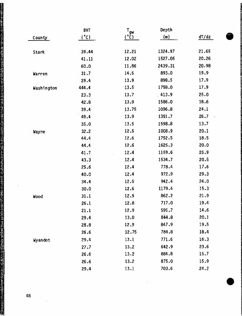
Stark
Warren
Wash i n gton
Wayne
Wood
Wyandot
BHT
("C)
39.44 41.11 60.0 31.7 29.4
444.4 23.3 42.8 39.4 49.4 35 .O 32.2 44.4 44.4 41.7 43.3 25.6 40.0 34.4 30.0 31.1 26.1 21.1 29.4 28.8 26.6 29.4
27.7 26.6
26.6 29.4
Tgw ("C)
12.21 12.02 11.86 14.5 13.9 13.5 13.7 13.9 13.75 13.9 13.5 12.5 12.6 12.6 12.4 12.4 12.4 12.4 12.5 12.6 12.9 12.8 12.9 13.0 12.9 12.75 13.1 13.2 13.2
13.2 13.1
Depth
(m 1
1324.97 1527.05 2439.31
893.0 898.5
1758.0 413.9
1586 .O 1096.8 1351.7 1598.8 1008.9 1752.5 1625.3 1159.6 1534.7 778.4 972.9 942.4
1179.4 862.2 717.0 595.7 844.8 847.9 784.8
771.6 642.9 884.8 875.0 703.6
dT/dz
21.65 20.26 20.98 19.9 17.9 17.9
25.0 18.6 24.1 26.7
13.7 20.1 18.5 20.0 25.9 20.5 17.6 29.3 24.0 15.3 21.9 19.4
14.6 20.1 19.5 18.4
16.3 23.6 15.7 15.9 24.2
48

APPENDIX B
BOTTOM-HOLE TEMPERATURES I N O I L AND GAS WELLS
I N PENNSYLVANIA AND ADJACENT AREAS OF
MARYLAND AND WEST V I R G I N I A
49

BHT County ("C)
Armstrong
Beaver
Bedford
A1 1 egheny 18.56 31.67 71 .ll 35.00 25.83 72.78 29.44 62.78 32.22 22.00 34.28 22.22 30.00 30.00 26.67 37.22 55.17 47.22 54.44 49.44 60.83 19.89 17.78 86.67 55.56 37.78 47.22 45.00 56.11 45.00 35.56 35.56 36.67
Depth (m) dT/dz
12.33 12.19 12.22 12.39 12.06 12.28 11.14 12.15 12.23 12.11 12.24 12.11 12 .oo 11.69 11.78 11.53 11.72 11.56 11.86 11.28 11.39 11.81 11.81 11.86 11.83 11.44 11.54 11.42 11.22 12.09 11.61 11.61 11.72
565.4 955.5 2407.9 1236 .O 778.5 2311.6 931.5 2234.5 1175.9 992.4 1097.3 928.1 944.9 990.0 879.0 975.4 2194.6 2051.3 2273.8 2014.7 1398.4 444.7 448.1 2389.6 2826.4 1310.6 1615.4 1839.2 2199.1 2128.4 853.4 1531.6 1502.7
11.63 21.05 24.77 18.76 18.42 26.52 20.31 22.97 17.36 10.29 20.66 11.26 19.69 19.08 17.55 27.19 20.08 17.65 18.98 19.23 36.15 19.51 14.30 31.71 15.64 20.57 22.51 18.56 20.70 15.69 29.10 15.95 16.94
dT/dzb
21.73 25.97 19.34 18.77 27.80
24.11 17.93 10.74 21.30
C
20.34 C
17.86 C
21.09 18.35 19.95 19.98 37.03
33.18 16.63 21.26 23.41 19.31
16.33 29.53 16.66 17.44
50

BHT County ("C)
B1 a i r 47.78 58.33 46.11 64.44 34.06
Bradford 98.89 58.89 35.00 45.83 36.39
But1 er 20.44 35.00 21.39 19.78 25.39 28.78 34.72 51.67
C ambr i a 65.56 34.72 63.89 84.17
60.56 65.00 66.39 72.50 70.00 73.89 69.72 73.89 86.39
Cameron 59.44 43.33
e
Depth (m 1
11.92 11.94 12.08 12.06 11.78 10.22 10.17 10.37 10.11 10.01 11.64 11.31 11.06 11.70 11.92 11.81 11.22 11.25 12.36 12.33 12.17 12.39
12.50 12.44 12.39 12.39 12.36 12.11 12.11 12.17 12.17 11.06 10.97
1774.9 2822.4 2122.6 2164.1 1020.5 3914.5 2288.1 1227.1 2012.9 1402.1 527.3 1038.5 614.2 568.5 810.2 807.7 1689.8 2316.5 2468.9 1524.0 2225 .O 2718.8
2447.8 2923.0 2593.8 2606.0 2781.6 2503.6 2578.6 2432.3 2489.9 2036.1 1822.1
dT/dz
20.56 16.62 16.26 24.55 22.50 22.83 21.58 20.58 18.02 19.23 17.72 23.50 17.70 15.02 17.28 21.84 14.16 17.68 21.82 14.99 23.57 26.70
19.88 18.17 21.07 23.34 20.95 24.98 22.61 25.70 30.18 24.13 18.06
dT/dzb
21.38 17.66 16.93 25.76
24.10 22.10 21.17 18.71 19.76
24.20 18.07 15.38 17.60 22.21
C
22.89 15.69 24.73 17.95
19.29 22.10 24.47 22.22 27.17 23.70 26.93 31.58 25.02 18.79
I
51

BHT County ("C)
51.11 50.56 56.56 66.67 59.61 52.78 60.00 16.50 58.33 14.17
Carbon 44.17 41.11
Centre 58.06 60.00 70.00
C l i n t o n 54.44 21.56
C1 a r i on 25.56 14.78 19.67 24.44 21.11 23.89 29.31 32.22 23.61 22.00 16.67 19.28 23.33
23.33 25.28 28.89
Depth (m 1 dT/dz dT/dzb
11.14 11.15 11.06 11.00 11.06 11.06 11 .oo 11.00 11 .oo 11.00 11.39 11.42 11.67 11.61 11.33 11.39 11.28 11.06 11.17 11.03 11.17 11.17 11.33 11.33
11.33 11.08 11.22 11.04 11.28 11.17
11.17 11.17
11.22
1790.7 1872.4 1976.3 1983.0 1823.3 1984.6 2048.3
914.4 1964.4 766.3 978.4
1644.7 2468.9 2179.3 4773.8 2580.7
608.4 696.2 693.42 557.82 960.1 798.0 640.1 896.1
954.6 774.2 762.0 538.3 707.1 740.7
742.2 808.0
809.5
22.71 21.39 23.38 28.51
27.08 21.35 24.28 6.22
24.47 4.30
34.58 18.40 19.02 22.52 12.37 16.88 17.78 21.78
5.45 16.37 14.28 12.96 20.60 20.76
22.60 16.85 14.73 11.08 11.82 17.13
17.10 18.15
22.68
24.26 29.53
28.08 C
25.18 6.60
25.38
35.51 19.16 19.98 23.64 13.11 17.74
22.17 5.67
16.37
*
C
13.23
C
11.41 12.11 17.46
17.42 18.47
52

BHT County ("C)
23 .a9 20.83 29.17 23.89 20.56 22.50 21 .a1
19 .za 28.75
17.36
20.56 20.00 20.28 22.78 31.67 21.11 17.22 28.94 68 .a9 60.14 51.94 53.33
56.11 42 . 78 52.78 67 -78 C 1 earf iel d 65.56 70.33 73 .a9 75.56 56.11 63.33 65.56
Depth (m 1 dT/dz dT/dzb
11.17 11.17 11.06 11 -06 11.31 11.11 11.04 11.03 11.06 11.17 11.10 11.10 11.17 11.09 11 .oo 10.98 10i97 10.96 11.06 11.06 11.06 11 -06
11 .oo 11.00 10.94 12.11 11.28 11.32 11.67 12.00 11.67 11.67 11.67
869.6 789.4 758.3 574.2 765 .O 634.0 865.6 636.4 939.7 634.0 752.9 1525 .a 666 .O 794.3 749.2 792.5 369.7 912.3 2409.7 1760.2 1767 .a 1699 -6
2265.6 '1645.9 2966.0
2136.6 ,2392.7 2498.4 2254.9 2380.5 2270.8
15.16 12.74 24.88 23.60 12.58 18 .a7 12.89 10.45 9.04 29.14 13.09 5.95 14.34 15.30 28.75 13.30 18 .42 20.40 24.31 28.38 23.54 25.33
20.18 19.67 21.61 22.27 29.56 28.02 26.34 25.75 19.98 21.99 24.05
29.20 13.58
20.73 25.47 29.42
C 26.29
20.69 20.47 22.43 23.36
26.98 20.99 23.06 25.03

Craw f ord
E l k
BHT County ("C)
62.22 75.56 78.33 67.22 67.22 60.00 78.33 68.11 73.33 70.28 58.33 33.33 37.78 36.11 38.33 35.00 33.33 36.11 31.67 34.44 43.33 34.44 36.67 38.33 43.33 45.00 42.22 45.00 59.44 62.94 74.44 48.33 56.78
Depth (m 1 dT/dz dT/dzb
11.67 11.39 11.89 11.78 11.48 11.32 11.44 11.28 11.67 11.30 11.17 11.03 10.89 10.83 10.91 10.89 10.78 10.92 10.92 10.92 11 .oo 10.93 10.89 10.91 10.89 10.92 10.72 10.74 11 .ll 11.18 11.19 11.06 11.06
2313.4 2211.3 2484.1 2461.3 2188.6 2354 .O 2316.5 2042.2 2315.0 2301.2 1996.4 1200.6 1206.7 1323.1 1233.2 1248.5 1314.3 1250.0 1163.1 1233.2 1242.7 1293.6 1312.2 1294.2 1609.6 1460.3 1006.7 1553.0 1874.4 2194.6 2127.5 1978.2 1979.3
22.14 29.42 27.08 22.81 26.50 20.95 29.26 28.25 26.99 25.97 23.99 19.06 22.86 19.55 22.80 19.80 17.57 20.66 18.32 19.56 26.67 18.62 20.11 21.70 20.55 23.84 19.38 22.50 6.21 23.92 30.16 19.14 23.46
23.24 30.81 28.36 23.92 27.78 21.99 30.63 29.27 28.28 27.21 24.59 19.63
23.44 20.37 18.09 21.25 18.87 20.13 27.39 18.16 20.68 22.31 21.37
C
20.16 23.39 27.18 24.50
19.88 24.33
54

BHT County ("C)
E r i e
66.67 54.44 57.22 18.61 23.33 56.44 68.33 59.17 61 .ll 44.44 30.56 40.56 22.89 30.56 32.78 20.00 43.33
Fayet te 39.44 74.44 27.61 37.78 75.56
24.72 74.44 69.44 79.44 70.56 33.50 27.22 65.56
64.44 23.89 68.61
Depth (m 1 dT/dz dT/dzb
11.22 11.00 10.97 10.89 10.89 11.14 11.02 11.04 11.11 10.87 10.83 10.69 10.94 10.94 10.94 10.68 10.74 12.19 13.18 13.33 13.33 13.06
13.00 13.06 13.06 12.78 12.18 12.19 12.85 12.56
12.91 13.33 13.18
2008 0 1969.0 1865.4 664.5 492.3
1966.9 2471.9 1859.3 2179.3 1241.1 1148.5 1361.8 1068.6 874.8
1001.3 378.0
1260.3 1197.3 2545.7
911.4 1173.5 2011 -7
701 .O 2069.6 2380.5 2816.7 2148.8
972.9 1219.2 2727.4
2684.4 807.7
2427.4
28.04 22.41 25.21 12.18 26.95 23.39 23.47 26.32 23.27 27.73 17.64 22.43 11.51 23.23 22.49 26.81 26.50 23.35 24.36 16.21 21.39 31.55
17.48 30.11 24.00 23.93 27.56 22.61 12.09 19.65
19.42 13.58 23.13
23.25 26.14 12.18
C
24.27 24.59 27.29 24.41 28.46 18.19 23.04
23.59 23.17 27.39 27.20
C
25.54 16.52 22.05 32.69
17.85 31.20 25.18 25.35
23.32 12.55 20.62
20.39 13.89
C

Forest
Ful ton Greene
BHT County ("C)
90.00 80.56 72.50 69.44 71.67 103.61 73.33 75.00 14.11 46.11 46.11 17.39 54.44 31.11 26.56 32.78 26.67 32.78 32.89 75.83
Indiana 35.00 75.56 76.67 80.00 80.83 71.11 52.22 28.89 36.67 21.89 81.67 58.44 26.83
13.24 13.39 13.33 13.33 13.14 13.24 13.19 13.24 10.89 10.83 10.83 10.86 10.89 11.11 13.41 13.39 13.33 13.34 12.59 12.96 12.36 12.42 12.25 12.27 12.36 12.36 12.33 12.31 12.14 12.42 12.42 12.44 12.34
Depth (m 1
3291.8 2910.8 2407.9 2133.6 2407.9 3627.1 2313.4 2417.1 645 .O 1837.0 1870.6 314.2 2086.1 874.8 910.1 993.6 951 .O 975.7 2331.7 2639.6 1164.3 2581.7 2455.2 2471.9 2118.4 2285.4 1828.8 960.1 1066.8 678.1 2255.5 2286.0 1066.8
dT/dz dT/dzb
23.53 23.32 24.89 26.68 24.62 25.13 26.34 25.88 5.24 19.53 19.17 23.02 21.19 23.69 14.95 20.13 14.48 20.56 8.77 24.10 19.97 24.75 26.57 27.74 32.80 26.06 22.18 17.84 23.66 12.84 31.12 20.39 13.98
24.91 C
28.00 25.82 26.57 27.63 17.14 5.47 19.92 19.92
C
21.98 24.06 15.25
C
9.34 25.26 20.58 25.93
29.05 33.96
32.59 21.43 14.50
56

BHT County ("C)
54.44 74.44 73.33 20.56 62.78 68.33 68.89 72.22
Jef ferson 21.83 28.56 23.72 42.50 69.72 63.33 44.72 66.67 39.17 40.83 71.67 75.56 38.89 53 - 33 34.28 33.89 29.72 74.72 64.44
Juniata 58.89 Lackawanna 40 00
Lawrence 60.00 47.78
Luzerne 30.00 24.44
Depth (m 1 dT/dz dT/dzb
12.35 12.50 12.47 11.78 11.94 11 -81 11.88 11.83 11.08 11.11 11.42 11.53 11.53 11.46 11.10 11.71 11.58 11.58 11.58 11.56 11.60 11 -56 11.69 11.67 11.61 11.69 11.53 10.91 10.14 11.04 11.08 10.49 10.56
2334.2 2530.1 2301.2 1001 .o 2203.7 2329.0 2097.9 2350.0 804.7 911.4 417.6 1219.2 2212.8 2171.7 917.4 2202.2 1219.2 1219.2 2177.8 2280.5 1100.3 2261.6 1036.3 1103.4 1127.8 2170.2 2234.2 2659.4 1648.4 1453.9 1478.3 1118.6 1402.1
18.27 24.95 26.80 9.04 23.39 24.59 27.58 26.03 13.89 19.80 31.79 26.06 26.67 24.23 37.91 25.31 23.20 24-61 27.98 28.44 25.51 18.72 22.45 20.71 16.51 29.46 24.01 18.25 18.46 34.39 25.35 17.93 10.13
19.22
24.55 25.78 28.58 27.28
20.13 32.42 26.77 27.94 25.41 38.92 26.54 23.86 25.29 29.32 29.79 26.23 19.68 23.13 21.34 17.05 30.85 25.18 19.15 19.20 35.24 26.01 la. 4% 10.48
57

BHT County ("C)
Lycomi ng 55.56 32.22 61.67 58.89 57.89 59.17 81 .ll 54.44
McKean 48.06 75.28 47.78 50.56 62.22 60.00 50.00 10.11 42.78 47.78 40.00 55.56 43.89 24.06
Mercer 40.56 43.33 50.00 43.33 35.00 47.22 40.28 43.33 43.50 46.11 64.44
58
Depth (m 1 dT/dz dT/dzb
10.96 10.63 11.08 10.99 11.06 11.03 10.77 11.13 10.72 10.74 10.73 10.79 10.89 10.83 10.71 10.67 10.66 10.78 10.67 10.86 10.83 10.79 11.03 11.04 10.96 10.97 11.03 10.89 10.91 10.94 10.92 10.94 10.92
2024.5 1187.2 2407.9 2202.8 1813.6 2098.5 2474.4 2197.6 1264.9 3618.0 1399.0 1720.6 2002.5 1551.4 1438.4 1173.5 1140.0 1659.6 1219.5 2068.1 1492.6 585.2 1537.7 1560.6 1882.4 1618.5 1460.6 1661.2 1713.9 1749.6 1757.5 1539.2 2784.7
22.36 18.67 21.28 22.05 26.27 23.28 28.78 19.99 30.24 17.99 27.07 23.53 26.03 32.33 27.91 -0.49 28.95 22.71 24.67 21.94 22.61 23.91 19.59 21.11 21.07 20.38 16.86 22.28 17.45 18.84 18.87 23.31 19.44
19.23 22.32 23.13
24.14 29.45 20.99 31.02 19.04 27.77 24.42 26.98 33.51 28.62 -0.31 29.72 23.59 25.34 22.76 23.21 24.34 20.13 21.96 21.88 21.20
23.15 18.17 19.60 19.62 24.23 20.61

BHT County ("C)
40.56 Pike 103.89 Potter 56.67
60.83 46.67 46.94 60.00 53.33 58.33 55.00 59.44 52.22 47.78 54.44 47.22 46 11 40.56 55.00
Somerset 77 .OO 71.67 142.78 62.78 64.44 43.33 49.44 72.22 70.00 51.11 38.89 85.72 76.11
Sull i v a n 77.78 60.83
Depth (m 1
11.02 10.89 11 .oo 11 -06 10.79 11.04 10.98 10.89 10.93 11.06 11.06 10.83 10.81 10.81 10.78 10.78 10.78 11.06 12 .oo 13.00 12.94 12.83 12.58 12.67 12.47 12.50 12.66 12.64 12.44 12.52 12.39 10.52 10.52
1612.1 4239.8 1920.2 1941.6 1740.1 1539.2 1862.3 1877.6 2363.7 2133.0 2044.6 1566.7 1633.7 1600.2 1608.7 1565.1 1575.8 2088.5 2776.7 2407.9 6521 .O 2656.3 2612.7 1371 .O 1959 .O 2608.5 2255.5 2407.9 1493.5 2743.2 2802.0 2853.8 2192.7
dT/dz
18.67 22.09 24.17 26.05 20.99 23.79 26.76 22.98 20.32 20.90 24.02 26.94 23.06 27.80 23.09 23.02 19.27 21.35 23.67 24.68 19.94 19.02 20.08 22.89 19.16 23.17 25.77 16.18 18.07 26.98 22.99 23.82 23.27
dT/dzb
19.44 23.33 25.06 27.00 221.80
27.74 23.85 21.32 21.69 24.91 27.96 23.95 28.84 23.99 23.92 20.06 22.15 25.07
20.60
23.54 19.93 24.29 27.03
18.61 28.56 24.36
59

Venango
Warren
Washington
BHT County ("C)
Susquehanna 60.00 Tioga 65.56
53.06 79.44 38.33 52.22 52.22 70.00 48.89 26.17 30.00 47.78 45.42 53.3 45.56 48.89 21.11 16.67 30.00 16.67 40.56 41.67 48.06 44.44 63.89 43.33 73.06 80.56 25.28 73.33 17.50 33.33 39.44
Depth (m 1 dT/dz dT/dzb
9.89 10.92 10.89 10.92 10.80 10.81 10.75 10.94 10.89 10.91 10.91 10.94 10.94 10.98 10.96 10.96 10.89 10.86 10.89 10.79 10.73 10.65 10.78 10.78 10.63 10.74 11.97 11.97 12.11 12.06 11.97 12.17 12.00
2601.2 1808.4 1661.2 3138.5 1387.8 1584 .O 1681.0 2771.2 1845.6 634.0 760.2 1984.2 2002.8 2033.6 1935.5 2048.6 312.4 211.7 659.3 290.2 1418.5 1209.1 1770.9 1837.3 2478.0 1732.2 2475.0 2329.9 807.7 2590.8 723.9 1216.2 1338.1
19.49 30.73 25.86 22.05 20.29 26.66 25.13 21.55 20.94 25.29 26.16 18.85 17.48 21.14 18.16 18.80 36.26 32.07 30.39 22.63 21.56 26.32 21.42 18.63 25.84 19.15 24.99 29.83 16.94 23.93 7.97 17.85 20.99
20.43 31.84 26.83 23.33 20.85 27.66 26.08 22.82 21.74 25.72 26.57 19.59 18.17 21.94 18.88 19.52 37.01 32.07
22.14 27.02
26.05 19.91 26.18 31.23 17.27 25.08
18.41 21.59
60

BHT County ("C)
50.00 26.67 26.83 50.56
Wayne 73.89 32.78 32.50
Westmorel and 23.50 60.00 73.89 66.11 72.22 63.33 60.67 46.39 24.83 38.89 66.67 70.56 84.72 31.11 60.17
68.89 46.11 34.44 62.78
Wyoming Maryland
West V i r g i n ,,A 115.00 78 -89
Depth (m 1 dT/dz
12.36 12.13 12.11 12.16 10.13 10.21 10.17 12.00 12.13 12.44 12.76 12.47 12.42 12.33 12.25 12.28 12.44 12.37 12.50 12 -47 12.08 12.75
12.65 10.08 11.76 11.92 13.39 11.90
2004.1 890.0 813.5
1796.8 3733.8 1511 .8 1521 .O 895.5
2225 .O 2274.1 2414.0 2255.5 2171.7 2260.7
1386.8 640.1
1097.3 2514.6 2340.9 2356.9 1120.1 2539.3
2444 . 5 1243.0 1380.7 2167.1 5032.9 3166 .O
19.07 16.91 18.80 21.74 17.22 15.24 14.98 13.29 21.81 27.39 22.39 26.85 23.78 21.67
25.17 20.60 24.79 21.86 25.13 31.04 17.46 22.09
23.30 29.72 16.80 23.80 20.31 21.36
dT/dzb
19.14
18.21 15.68 15.42 13.57 22.91 28.70 23.49 18.15 24.96 22.76
25.85 21 .oo
22.93 26.35 32.50 18.03 23.18
24.44 30.48
' 1
61

APPENDIX B , (cont)
a Ground water temperature a t depth of 30.5 m.
b Geothermal gradient correction for the effects of dri l l ing.
Time Between Drillina ComDletion and Loaaina
Depth ( m ) 0 - 1 day 2 days
0 152.4 152.4 304.8 304.8 914.4 914.4 1524.0
1524.0 2133.6 2133.6 2743.2
> 2743.2
-1 0 1 2 3 4 5
C Borehole logged three or more days after completion of dri l l ing. No temperature correction was applied.
1 62

APPENDIX C
DEPTH/TEMPERATURE RECORD FROM WELL 3236,
WASHINGTON COUNTY, OHIO
63

Ob
DEPTH Topography
d Corrected ( m )
15.2 30.5 45.7 61 .O 76.2 91.4
106.7 121.9 137.2 152.4 167.6 182.9 198.1 213.4 228.6 243.8 259.1 274.3 289.6 304.8 320.0 335.3 350.5 365.8 381 .O 396.2 411.5 426.7
442 .O 457.22 472.4 487.3
64
76.2
103.6
134.1
161.5
192.0
219.5
249.9
280.4
307.8
338.3
368.8
399.3
426.7
457.2
Ob
TEMPERATURE C 1 imate
erved Corrected "C 1 ( " C )
11.92 12.12 12.35 12.57 12.85 13.08 13.33 13.60 13.88 14.18 14.52 14.86 15.21 15.42 15.53 15.82 16.22 16.64 16.95 17.24 17.49
13.42 13.71 14.04 14.37 14.73 15.12 15 . 52 15.94 16.21 16.38 16.72 17.18 17.65 18.01 18.35 18.66
17.77 19.00 17.99 19.27 18 . 25 19.59 18.51 19.87 18.73 20.15 18.90 20.37 19.06 20.58
19.23 20.81 19.49 21.12
19.79 21.43 20.11 21.81

DEPTH Topography
Observed Corrected (m) (m)
TEMPERATURE C 1 imate
Observed Corrected ( " C ) ("C)
502.9 518.2
533.4 548.6
563.9
487.7
518.2
20.49 20.89
21.32 21.79
22.24 22.69
23.18 23.70
21.88 23.78
65

APPENDIX D
DEPTH/TEMPERATURE RECORD FROM BARBERTON WELL,
SUMMIT COUNTY, OHIO

Depth ( m )
0
50
75
100
105
110
115
120
124
130
135
140
145
150
180
210
240
270
300
330
360
390
420
450
480
Temperature
5.42 '
("C)
9.83
12.79
12.47
12.61
12.62
12.65
12.69
12.79
12.87
13.00
13.24
13.06
13.50
14.40
15.13
15.82
16.39
16.88
17.69
18.43
19.33
20.27
20.63
21.19
Geothermal Gradient
( "C /km)
88.40
118.40
-12.80
28 .OO
2.00
6.00
8.00
20.00
16 .OO
26.00
48.00
-36 00
88.00
30.00
24.33
23.00
19.00
16.33
27.00
24.67
30.00
31.33
12.00
18.67
32.00
67

Depth ( m )
510
540
570
600
630
660
690
720
750
780
810
815
820
825
830
835
840
845
850
Temperature ( " C )
22.15
23.02
23.86
25.09
26.51
27.33
28.01
28.01
29.08
29.76
31.17
31.46
31.85
32.14
32.66
32.95
33.02
33.05
33.12
Geothermal Gradient
("C/km)
29.00
28 .OO
41 .OO
47.33
27.33
22.67
23.33
12.33
22.67
47 .OO
58.00
78 .OO
58.00
104.00
58.00
14.00
6 .OO
14.00
14.00 855
68
33.19

APPENDIX E
DEPTH/TEMPERATURE RECORD FROM MORRISON WELL,
VENANGO COUNTY, PENNSYLVANIA
69

DEPTH TEMPERATURE GEOTHERMAL GRADIENT
Ob- served
( m )
10.00
20.00
30.00
40.00
50.00
60.00
70.00
80.00
90.00
100.00
110.00
120.00
130.00
140.00
150.00
160.00
170.00
180.00
190.00
200.00
210.00
220.00
230.00
240.00
250.00
260.00
270.00
280.00
290.00
300.00
305.00
Ob- Topog. served
(m) ("C) -- 0.86 5.23
10.11 5.37
19.36 6.18
28.63 6.38
37.91 6.69
47.21 6.96
56.54 7.10
65.88 7.30
75.26 7.62
84.66 7.95
94.08 8.14
103.53 8.42
113.01 8.56
122.51 8.81
132.04 9.13
141.60 9.35
151.17 9.53
160.77 9.68
170.39 9.89
180.03 10.11
189.67 10.33
199.36 10.51
209.06 10.77
218.76 11.02
228.49 11.22
238.23 11.51
247.98 11.69
257.74 11.87
267.52 12.65
277.31 13.41
282.20 13.47
River ("Cl
5.23
5.68
6.20
6.40
6.72
6.99
7.14
7.34
7.67
8.01
8.21
8.49
8.64
8.90
9.23
9.46
9.65
9.81
10.03
10.26
10.49
10.68
10.95
11.22
11.43
11.73
11.92
12.11
12.92
13.71
13.77
C1 imate ('C)
5.02
5.28
5.67
5.81
6.13
6.46
6.70
7.01
7.47
7.93
8.25
8.63
8.88
9.22
9.63
9.92
10.17
10.38
10.64
10.91
11.18
11.40
11.71
12.01
12.25
12.58
12.80
13.02
13.86
14.68
14.75
Ob- zerved C/km)
44.00
51.00
20.00
31 .OO
27 .OO
14.00
20.00
32.00
33.00
19.00
28.00
14.00
25.00
32.00
22.00
18.00
15.00
21.00
22.00
22.00
18.00
26 .OO
25.00
20.00
29.00
18.00
18 .OO
78.00
76.00
12.00
River & River C1 imate Corr. Corr. ("C/km) ('C/km) --
44.00
53.00
20.00
32.00
27 .OO
15.00
20.00
33.00
34.00
20.00
28.00
15.00
25.00
34.00
23.00
19.00
16.00
22.00
23.00
23.00
19.00
27 .OO
27.00
21 .oo
30.00
19.00
19.00
81 .OO
79 .OO
12.00
26.00
39.00
14.00
32.00
33.00
24.00
31 .OO
46.00
46 .OO
32.00
38.00
25.00
34.00
41.00
29.00
25.00
21.00
26 .OO
27.000
27.00
22.00
31.00
30.00
24.00
33.00
22.00
22.00
84.00
82.00
14.00
River, Climate, & Topog. Corr.
('C/km)
28.11
42.16
15.10
34.48
35.48
25.72
33.19
49.04
48.94
33.97
40.21
26.37
35.79
43.02
30.33
26.12
21.88
27.03
28.01
28.01
22.70
31.96
30.93
24.67
33.88
22.56
22.54
85.89
83.76
14.31
70

APPENDIX F
DEPTH/TEMPERATURE RECORD FROM BOWSER WELL,
CLARION COUNTY, PENNSYLVANIA
7 1

DEPTH TEMPE RAT U RE
Observed ( m )
48.73
98.73
148.73
173.73
198.73
208 73
213.73
218.73
223.73
228.73
243.73
258.73
263.73
258 73
273.73
278.73
288.73
293.73
298.73
303.73
308.73
313.73
318.73
323 73
72
Topogo Corr .
( m )
50.37
102.01
153.56
179.73
205.06
215.34
220.48
225.62
230.76
235.90
251.30
266.70
271.83
276 96
282.09
287.21
297.47
302.59
307.71
312.84
317.96
323.08
328.20
333.32
Observed ( " C )
4.19
5.81
7.73
9.20
10.18
10.52
10.77
10.94
11.68
11.79
12.22
12.48
12.59
12.71
12.82
12.94
13.17
13.30
13.41
13.54
13.66
13 77
13.86
13.97
C 1 imate Corr .
( " C l
3.60
5.72
8.12
9.74
10.83
11.21
11.47
11.66
12 42
12.54
13-02
13.32
13.45
13.58
13.71
13.84
14.20
14.25
14.37
14.52
14.65
14.78
14.88
15.01
GEOTHERMAL GRADIENT River R River ,
Observed ("C/km)
32.49
38.40
58.80
39.20
34.00
50.00
34.00
148.00
22.00
28.70
17.30
22.00
24.00
22 .oo
24.00
23.00
26.00
22 .oo 26 .OO
24.00
22 .oo
18 .OO
22 .oo 22 .oo
C I imateU Corr .
("C/km)
42.49
48.00
64.80
43.60
38.00
52.00
38.00
152.00
24.00
32 .OO
20.00
26 .OO
26.00
26 .OO
26 .OO
26.00
30.00
24.00
30.00
26.00
26.00
20.00
26.00
26 .OO
Climaie, & Topog. Corr.
( "C/km 1
41.95
46.54
62.91
42.36
36.96
50.58
36.96
147.86
23.35
31.17
19.48
25.34
25.34
25.34
25.39
25.34
29.30
23.44
29.24
25.39
25.39
19.53
25.39
25.44

DEPTH
Observed ( m 1
328.73
333.83
338 73
343.73
348.73
353 . 73
363 ! 73
373 I73
388.73
403 I73 I
418 73
438 A 73 , I
453 I73
Topog. Corr.
( m 1
338.43
343.65
348.67
353.78
358.89
364.01
374.23
384.45
399.77
415.09
430.39
450.79
466.08
TEMPERATURE
Observed ( " C )
14.08
14.22
14.30
14.37
14.51
14.66
14.94
15.21
15.64
16.09
16.48
17.03
17.45
C 1 imate Corr.
( " C )
15.14
15.29
15.39
15.47
15.63
15.80
16.11
16.41
16.89
17.40
17.84
18.46
18.93
GEOTHERMAL GRADIENT River & River .
Ob served ( "C/km 1
27.45
16.33
14.00
28.00
30.00
28.00
27 .OO
28.67
30.00
26 .OO
27.50
28.00
C 1 imate Corr .
( "C/km)
29.40
20.40
16 .OO
32.00
34.00
31.00
30.00
32.00
34.00
29.30
31 .OO
31.30
Climate, & Topog. Corr.
( " C / k m )
28.74
19.92
15.66
31.31
33.20
30.33
29.35
31.33
33.29
28.76
'30.39
30.74
73

APPENDIX G
THERMAL CONDUCTIVITY OF CORE SAMPLES
FROM WELLS I N WASHINGTON, NOBLE,
AND MORGAN COUNTIES, OHIO

Depth (m)
34.1 108.6 130.2 169.5 175.4 192.9 196 .O 196.7 2-6.3 234.1 250.6
57.1 58.6 64.4 72.3
152.7 154.2 158.4 165.7 165.8 172.9 175.8
217.3 217.3
217.3 217.5 227.0
Thermal Conductivity R ( dry 1 K(wet)
(rncal /crnsec"C ) L i tho1 ogy
We1 1 2386. Washinaton County. Ohio
Ls ss ss Sh Sh Sh
ss Sh Ls s1 t s t Ls
5.53 5.95 6.44 2.80 3.54 4.22 8.56 3.53 5.11 4.14 7.18
5.73 7.95 7.16 2.88 3.47 4.22
10.41 3.52 5.22 4.01 7.69
We1 1 2181, Washington County, Ohio
ss Ls ss Mds t
ss Sh Sh s1 t s t
s1 t s t
ss Sh
Coal Coal
Coal Mds t Sh
6.64 4.13 7.00 6.44 7.85 3.78 4.51 3.82 3.75 6.98 4.96
0.93 1.13
0.77 4.82 3.48
9.39 4.98 8.51 6.88
10.14 3.83 4.74 4.10 4.09 8.19 5.19
0.98 1.19
0.812 4.93 3.53
Porosity ( % I
1.46 8.54 3.05 5.36 2.86 2.07 9.28 3.34 0.58 3.19
1.04
8.27 2.83 4.15 2.09 3.40 3.68 1.86 2.48 3.46 2.71 ---
3.53 2.58
3.51 2.78 ---
75

Thermal Conductivi ty W r y ) . K(wet) Porosity
L i tho1 ogy (mcal /cmsec"C 1. ( % I Depth
(m 1
106.2 129.4
53.6 59.7 89.3
117.9 127.3 139.3 140.1
152.7 163.1 164.9 165.6 171.7 178.3 184.4 194.1 229.3 229.3 231.2
100.0
122.2 163.4 183.8 219.7
76
Well 2387, Noble County, Ohio
s1 t s t 4.84 5.25 s1 t s t 5.93 6.29
Well 2176, Noble County, Ohio
Ls
Ls
s1 t s t ss Mds t ss SS
ss ss Mds t s1 t s t
ss Sh
s1 t s t
Sh Sh Sh
ss
7.11 5.65 5.00 4.72 3.53 7.81
8.23 7.81 4.68 4.58 5.15 8.05 3.62 4.38 4.06 4.20 4.31 8 .OO
7.36 5.73 6.01 5.40 3.42
10.29
10.47 9.85 5.52 4.53 5.54
10.20 3.52 5.01 4.16 4.46 4.53 9.02
Well 2177, Noble County, Ohio
Sh - 4.34 4.82
ss 7.06 9.39 ss 5.88 7.23
s1 t s t 5.96 6.28
ss 9.53 11.70
--- 1.74
1.94
0.60 6.00 4.60 5.11
10.65
9.36 11.36 4.15 ---
2.61 8.68 4.82 4.24 3.62 2.22 2.57 2.82
3.77
10.82 3.87 2.88
20.24

Depth (m 1
69.4 78.6
124.6 155.0 174.9 182.9 200.2 214.1 217.9 242.0 267.9
70.7 85.6 93.6
104.1 168.2 187.7 200.6 222.4
232.9 234.8
244.8 247.2
248.3 251.2
Thermal Conductivity w r y 1 K(wet)
( m a l /cmsec"C ) L i tho1 ogy
Well 2178, Morgan County, Ohio
Sh Sh Sh ss ss Mds t s1 t s t s1 t s t SS
Sh s1 t s t
5.15 4.14 3.67 7.67 8.09 4.30 6.20 4.77 7.04 4.60 4.86
5.95 4.40 3.76 9.72 9.70 4.32 6.36 4.83 8.11 4.68 4.98
Well 2180, Morgan County, O h i o
Mds t s1 t s t Ls ss s1 t s t Sh Sh s1 t s t
4.19 4.42 5.54 8.30 3.41 3.15 3.78 6.02
4.44 4.74 5.50 9.24 3.41 3.35 4.04 6.08
Well 2182, southeastern Ohio
Sh 4.09 4.12 s1 t s t 4.33 4.38
ss 9.25 11.05 Mds t 5.92 5.92 s1 t s t 6.80 6.97 Mds t 6.12 6.24
Porosity ( % I
--- 1.13 ---
12.14 10.96 3.97 1.84 3.31 2.82 2.51 ---
3.80 5.15 2.33 2.72 3.77 ---
2.57 4.42
2.40 2.42
10.76 2.41 2.01 2.82
77

APPENDIX H
THERMAL CONDUCTIVITY OF CORE SAMPLES FROM BARBERTON WELL,
SUMMIT COUNTY, OHIO
78

Depth (m 1
113.9 117.4 118.3 121.1 123.5 126.9 129.6 132.7 135.7 138.8 142.1 147.6 782.6 786.9 791.8 796.7 801.5 806.1 813.7 816.2 820.2 825.9 830.8 835.7 840.3 846.4 850.3 855.2
L i tho1 ogy
Sh
Sh Sh
Sh
Sh
Sh Sh
Sh
Sh
Sh Sh
Sh Ls
Ls Ls
Ls Ls
Ls Ls
Ls Ls Ls Ls
Ls Ls
Ls Ls
Ls
Thermal Conduct iv i ty m r Y 1 K (wet )
(mcal /cmsec"C )
1.38 3.00 3.22 2.25 2.46 2.63 2.35 2.83 2.00 1.37 1.25 1.64 5.64 5.45 6.12 5.24 3.50 5.30 3.84 4.89 4.56 5.46 6.06 5.67 6.23 5.33 5.90 5.81
--- 4.43 3.91 2.93 2.94 --- ---
3.14 --- --- ---
3.40 5.64 5.55 5.90 6.74 5.00 7.10 3.91 4.73 4.66 5.87 6.47 6.02 6.63 5.46 6.15 6.21
P o r o s i t y
--- 1.36 1.09 1.74 1.41 --- ---
1.99 --- --- ---
1.26 2.03
21.45 .74 .69 .48 .78
5.18 1.91 1.66
.95
.69 2.17 1.62 1.11
1.33 1.42

APPENDIX I
THERMAL CONDUCTIVITY OF CORE SAMPLES
FROM OTHER WELLS I N OHIO
80

Thermal Conductivi tv
Depth (m 1
394.9 398.0 401.1 550.5 556.6 557.2 838.8 927.2 930.3 930.3 931.8 936.4
1217.6 1218.5 1220.0 1221.2 1223.1 1223.1 1224.6 1226.1 1227.6 1220.2 1231.0
K(dry) K(wet)a L i tho1 ogy (mcal/crnsec"C)
Wilson w e l l , Fayet te County, Ohio
Ls Ls Ls Dol Dol
Do 1
Sh ss SS
ss ss Ls
5.21 4.75 4.32 5.60 6.82 7.47 2.67 5.31 3.98 3.75 5.45 7.84
7.01 8.96 5.06 9.96 8.18 7.59 3.32 7.23 7.83 7.59 7.30 10.24
H e s a w e l l , Morrow County, Ohio
Ls Ls Ls Ls Ls Ls Ls Ls Ls Ls Ls
8.45 7.01 8.53 6.82 6.82 6.77 7.21 6.05 8.24 8.46 7.16
9.16 8.17 9.72 9.03 9.03 8.07 8.92 8.20 9.42 28.76 7.22
Porosi ty ( %)
1.90 2.39 1.32 4.13 9.94 4.97 1.33 10.73 11.20 9.30 10.30 5.082
5.48 6.72 8.08 2.24 2.24 5.13 6.10 3.58 3.29 2.95 5.02
81

Thermal Conductivi t v
Depth (m)
37.9 46.1 51.5 61.1 68.6 76.3 82.6 99.1 107.1 113.5 114.1 129.3 137.6 143.0
K(dry) K(wet)a Li thology (mcal /cmsec"C 1
U. S . Gypsum well, Ottawa County, Ohio
Dol Do 1 Dol Dol Dol Dol Dol Dol Dol Sh
Sh Do 1 Dol Sh
12.58 8.84 9.13 12.27 12.02 10.04 10.50 10.37 9.17 2.55 2.60 10.77 10.68 2.56
13.49 11.92 10.55 13.17 12.80 12.26 12.832 12.90 9.70 --- --e
12.27 11.60
---
Poros i ty ( % I
4.84 5.62 9.06 5.88 3.56 10.33 7.86 9.74 9.89 --- --- 5.64 3.58 1.33
aSeveral green s h a l e s d isaggrega ted dur ing the vacuum-saturation process . Another was destroyed during pressur ized-conduct iv i ty measurement. Paraffin b indings d id n o t keep these s h a l e s from being des t royed .
82
APPENDIX J
THERMAL CONDUCTIVITY OF CORE SAMPLES
FROM THE WELLS I N CLARION AND
VENANGO COUNTIES, PENNSYLVANIA
83

Depth (m) -
241.4 244.4 247.3 250.0 351.2 251.9 286.7 290.3
258.9 287.1 293.8 298.1 299.3 301.1
250.5 251.8 253.3 255.1 256.5
226.3 248.7
263.9 264.7 267.9
L i tho1 ogy
ss ss ss ss Sh Sh ss Cgl
ss ss ss ss ss ss
ss ss ss ss ss
Cgl Sh
Sh Sh ss
Thermal Conductivity Porositya Sonic Velocityb K(dry) K(wet) K(wet) Vacuum 16-day am.
- (mcal /cmsec'C) ( %I ( %) (m/sec 1 Vacuum satur. 16-day am. satur. satur. sa tur .
Bankson well , Venango County, Pennsylvania
7.36 9.38 9.37 6.48 3.46 3.42 8.342 9.50
8.77 8.44 6.94 9.24 7.99 5.78
8.14 8.45 9.53 6.25 8.14
11.58 3.89
4.30 4.94 6.25
8.78 10.49 10.44 7.24 --- ---
9.28 11.27
2.75 5.98
13.95 13.95 ---
--- 8.67
10.65
Marsh we1 1 Venango County, Pennsyl vanf a
10.24 9.39 9.55 8.35
10.40 10.07 8.49
7.41 2.78
15.32 7.93 9.02 6.94
Hazlett well Venango C o u n j , Pennsylvania
9.60 11.58 9.58 10.40
10.61 9.36 7.43 14.13 8.67 8.86 3.68
Reed we1 1 Venango County, Pennsylvania
11.79 4.67
5.25 3.71 7.35
4.39 4.28
4.18 2.86 4.58
3.42 4063.9 4417.5 4354.4 4175.5 4293.1
4515.6 3672.2 3650.3 3705.8
4.52 3142.2
4262.9 3907.8
4354.4 3907.8 4532.4
84

Depth (m 1
219.5 222.8 224.1'' 269.0 271 .O 272.0 280.9 282.1 283.1 285.1 286.2 287.4 288.8 290.0 291.4 293.2 '294.4 296.3 308.3 310.0 323.8 326.5 334.2
340.2 346.3 349.3 586.2 589.2
Thermal Conductivity Poros 5 tya Sonic Vel oci tyb K(wt 1 K(wet ) Vacuum 16-day am. KO Vacuum satur. 16-day atm. satur. satur. satur.
l i thology
Sh
Cgl sg1 ss ss2 ss ss s1 t s t s1 t s t Sh Sh ss ss ss ss ss ss ss s1 t s t
Cgl Sh ss s1 t s t
s1 t s t
Cgl Sh Sh s1 t s t
4.67 11.14 10.32 7.92 7.68 5.91 6.60 7.57 5.36 3.85 3 .48 7.32 6.59 6.85 5.51 5.32 6.37 6.58
7.85 5.43 8.55 7.42
8.21 9.98 4.72 3.33 7.48
8.25
Bwser well, Clarion County, Pennsylvania
4.63 --- 1.86 12.99 6.00 11.29 6.40 10.38 7.83 7.77 7.77 0.71 6.84 4.99 6.65 --- 2.26 8.03 --- 1.27 --- --- 4.44
3.83 3.37 3.20 3.52 3.48 1.99 9.27 4.19 7.58 2.66 8.23 5.53 6.40 2.75 5.76 5.88 1.77 7.00 7.20 2.09 7.86 4.68 8.59 8.32 0.89
8.91 --- 1.20 5.63 5.71 2.00
10.08 10.06 1.99 8.52 3.30
8.27 8.37 1.70 11 .w 6.58 4.82 4.84 0.67 3.31 3.31 3.72 7.91 7.81 1.69
1.94
2.41
--- 1.27 ---
4.69 3.92
2.97 3.34
2.31
1.20 3.67
3.74
3.39
2.85 5.42 2.30
W s e c I
4063.9 4629.9 4493.4 3825.8 4313.2 4594.9 4063 e9 4701.2 4618.3 4313.2 4375.1 4417.5 4406.8 4375.1 4537.9 4549.1 4526.6 4471.4 4375.1
5080.1 4629.9
465.3 4665.3
4493.4 4812.5 4460.4 4174.8 4495.5
85

Depth (m1 -
257.6 260.9 279.2 283.8 294.6 295.4 291.1 311.5 312.7 315.0 334.7 337.1
L i tho1 ogy
s1 t s t ss Sh ss Cgl ss
QJl c!31 Cgl ss ss Sh
Therm - mduc ti v i ty Poros i t y Sonic Velocityb K(dry1 K(wet1 K(wet1 Vacuum 16-day atm.
Vacuum satur. 16-day a b . satur. satur. satur. (mcal /cmsec'C 1 ( %1 (% 1 W s e c 1
Bowser well, C la r ion County, Pennsylvania (continued)
Wile well , C lar ion County, Pennsylvania
8.28 8.72 8.91 11.17 3.53 3.46 7.56 8.87
10.02 11.40 9.63 10.17 7.62 8.35
12.69 12.81 10.78 11.84 9.92 11.63 7.79 8.53 4.73 4.75
8.99 0.92 8.08
3.47 1.15 3.15 4.30 2.57
--- 1.22 3.24
11.71 2.10 5.83
8.56 2.76 --- 5.55
2.24 4293.1 4010.6
3.34 4449.8 ., 4354.4 . e n
5277.9 2902.9
1.22 2930.7 4827.1
3.12 4876.8 4618.3
3.53 4218.7 --- 4800.0
aThe c u t - o f f poros i ty w i t h the vacuum-saturation method i s 2.5% Fourteen o f the 18 samples having poros i t ies o f less than 2.5% showed a mean increase i n poros i ty o f 2.87% when saturated under atmo- spheric pressure f o r 16 days.
bThe man o f the 1-ft and 3 - f t spacing values on the sonic-velocity logs was used.
86

APPENDIX K
RADIOGENIC ELEMENTS AND HEAT PRODUCTION I N CORE
AND OUTCROP SAMPLES FROM OHIO,
PENNSYLVANIA, AND NEW JERSEY
87

Location Map No. ‘County t e
1
2 3 4
5
6 7
8
9
10
11 12
13
14
15
16 17
OHIO - S m i t Barberton
Shale
Faye t te Morrow Granite Morrow
PENNSYLVANIA
Clar ion Bowser
Venango Bankson Reed
Clar ion Wile
E r i e
Berks F1 eetwood
Birdsboro Birdsboro
Boyer town
Mana towny
North- ampton Easton
Easton Easton
Li thology Analysta
Shale Shale Shale I Shale Amphibol i te
Pegma ti te
Shale Shill e Shale Shale Shale S i l t Shale Shale Shale Shale
Quartz-mica sch is t
Igneous Igneous Igneous Igneous Igneous Igneous Igneous
Igneous Igneous Igneous
Igneous Igneous Igneous Igneous Igneous Igneous
1 1 1
1 1 1 I
1 1 1 1 - 1
1 1 1 1
1 2 2 1 2 2 2 2
2 2 2
1 1 2 2 2 2
2.10 11.4 4.98 1.00 < 0.9 8.19 2.58 13.4 5.07
2.80 9.8 3.28 1.48 8.5 7.48 1.60 1.0 2.11 15.6 3.54 1.06
4.41 16.3 2.23 3.75 16.8 2.62 2.97 12.3 2.37 3.62 14.5 2.79 4.01 17.3 3.13 4.52 - 20.3 2.04 3.67 16.3 2.92 3.82 14.9 2.82 4.10 15.4 2.87 3.73 15.5 2.48 3.41 14.5 3.05
3.55 11.12 0.97 7.54 3.58 1.63 7.04 1.91
1.83 7.63 0.95 1.27 4.57 2.87 2.17 1.47 1.06 0.85 0.47 0.35 0.32 1.82
1.78 1.36 4.21 1.09 7.31 3.87 5.38 13.55 0.12
4.26 12.2 34.67 15.1
0.93 0.06 0.98 4.01 - 9.32 2.68 7.92 24.86 6.01 4.28 12.43 4.60
Heat K20 Generation - (%I (ycal/g/yr)
3.83 < 0.93
4.58 4.01
2.80 1.46 1.76 5.42 6.12 2.03 3.34
7.10 6.81
5.27 6.29 7.23 7.91 6.73 6.53 6.85 6.49 6.21
8.90 7.22 3.18 3.11
5.45 4.33 2.18 1.93
1.07 0.81
2.71 3.30 6.67
6.43 7.29 5.84 29.9
1.08 5.51
12.38 6.85
88
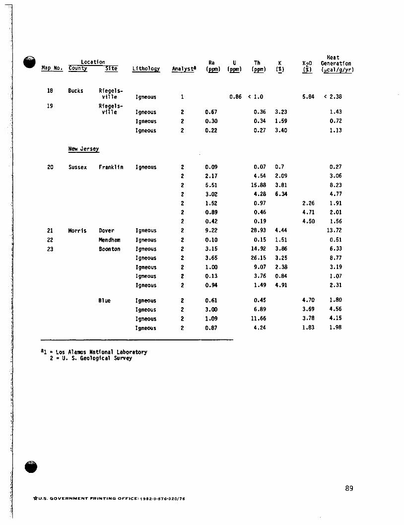
Ma - Location
S i te g - County hol ogy
18 Bucks
19
Riegels-
Riegel s- v i l l e Igneous
v i l l e Igneous Igneous Igneous
20
21 22 23
New Jersey
Sussex Franklin
Morris Dover Mendham Boon ton
E1 ue
9
1
2 2 2
Igneous 2 2 2 2 2 2 2
Igneous 2 Igneous 2 Igneous 2 Igneous 2 Igneous 2 Igneous 2 Igneous 2
Igneous 2 Igneous 2 Igneous 2 Igneous 2
Ra U Th K
0.86 < 1.0
0.67 0.36 3.23 0.30 0.34 1.59 0.22 0.27 3.40
0.09 2.17 5.51 3.02 1.52 0.89 0.42 9.22 0.10 3.15 3.65 1 .OO 0.13 0.94
0.61 3.00 1.09 0.87
0.07 0.7 4.54 2.09 15.88 3.81 4.28 6.34 0.97 0.46 0.19 28.93 4.44 0.15 1.51 14.92 3.86 26.15 3.25 9.07 2.38 3.76 0.84 1.49 4.91
0.45 6.89 11.66 4.24
al = Los Alamos National Laboratory 2 = U. S. Geological Survey
Heat K20 Generation - ( X I Iwcal/g/yr)
5.84 < 2.38
1.43 0.72 1.13
0.27 3.06 8.23 4.77
2.26 1.91 4.71 2.01 4.50 1.56
13.72 0.51 6.33 8.77 3.19 1.07 2.31
4.70 1.80 3.69 4.56 3.78 4.15 1.83 1.98
89 *U.S. GOVERNMENT PRINTING OFFICE: f 982-0-576-020/76