Geotechnical Slope Stability of the Este MSW...

UNIVERSITA’ DEGLI STUDI DI PADOVA

ICEA Department

MSc in Environmental Engineering

Master Thesis

Massimo Trivellato

Geotechnical Slope Stability of the Este MSW Landfill

Supervisor

Prof. Marco Favaretti

Academic Year 2013-2014

Un ringraziamento sincero ai miei genitori,

Gianpietro e Loredana

- 5 -

INDEX

Introduction .......................................................................................................................... - 9 -

1. Italian regulation about landfill slope stability ........................................................... - 10 -

2. Site description ............................................................................................................... - 11 -

2.1 Geographical Information .............................................................................................. - 11 -

2.2 Stratigraphy and Structure ............................................................................................. - 13 -

2.3 Hydrological properties ................................................................................................. - 14 -

2.4 Climate of the site .......................................................................................................... - 16 -

2.5 Seismology ..................................................................................................................... - 17 -

2.6 S.E.S.A. waste treatment activities ................................................................................ - 18 -

2.7 S.E.S.A. landfill description .......................................................................................... - 20 -

2.7.1 General information ............................................................................................. - 20 -

2.7.2 Principal administrative deeds ............................................................................. - 21 -

2.7.3 Sectors and subsectors ......................................................................................... - 22 -

2.7.4 Bottom liner systems ........................................................................................... - 26 -

2.7.5 Top cover systems ............................................................................................... - 26 -

2.7.6 Biogas management ............................................................................................. - 28 -

2.7.7 Leachate management ......................................................................................... - 30 -

2.7.8 Monitoring and control plan ................................................................................ - 31 -

3. General slope stability concepts .................................................................................... - 33 -

3.1 Introduction .................................................................................................................... - 33 -

3.2 Factors of influence........................................................................................................ - 34 -

3.3 Types of landfill’s failure............................................................................................... - 36 -

3.4 Seismic contribution ...................................................................................................... - 40 -

4. Slope Stability Analysis methods .................................................................................. - 43 -

4.1 Introduction .................................................................................................................... - 43 -

4.2 General concepts of Limit Equilibrium Methods .......................................................... - 44 -

4.3 LEM – Method of slices ................................................................................................ - 47 -

4.3.1 General formulation ............................................................................................. - 50 -

4.3.2 Fellenius method/OMS ........................................................................................ - 51 -

- 6 -

4.3.3 Bishop’s rigorous method .................................................................................... - 52 -

4.3.4 Bishop’s simplified method ................................................................................. - 53 -

4.3.5 Janbu’s simplified method ................................................................................... - 53 -

4.3.6 Janbu’s generalized method................................................................................. - 55 -

4.3.7 Morgenstern – Price method................................................................................ - 55 -

4.3.8 Spencer’s method ................................................................................................ - 55 -

4.3.9 Lowe – Karafiath’s method ................................................................................. - 56 -

4.3.10 Corps of Engineers method ............................................................................... - 56 -

4.3.11 Sarma’s method ................................................................................................. - 56 -

4.3.12 General limit equilibrium formulation .............................................................. - 57 -

4.3.13 Considerations on the interslice force function ................................................. - 59 -

4.3.14 Summary of the method of slices approaches ................................................... - 60 -

4.4 General concepts of Finite Element Method ................................................................. - 62 -

5. Definition of the input sections and parameters ......................................................... - 64 -

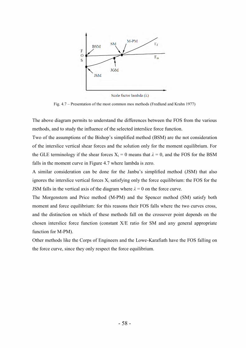
5.1 Chosen landfill sections for the calculation ................................................................... - 64 -

5.2 Geotechnical input data.................................................................................................. - 67 -

5.2.1 Material properties ............................................................................................... - 67 -

5.2.2 Waste properties considerations .......................................................................... - 68 -

5.2.3 Waste properties for Este’s landfill ..................................................................... - 72 -

5.2.4 Pore water pressure .............................................................................................. - 73 -

5.2.5 Reinforcement of soil – structure interaction ...................................................... - 73 -

5.2.6 Imposed loading .................................................................................................. - 75 -

6. Calculation procedure using LEM software: SLOPE/W ........................................... - 76 -

6.1 Introduction .................................................................................................................... - 76 -

6.2 Slip surface shapes ......................................................................................................... - 77 -

6.2.1 Grid and radius method ....................................................................................... - 77 -

6.2.2 Entry and exit method.......................................................................................... - 79 -

6.3 Analysis of section 4-4................................................................................................... - 80 -

6.3.1 Stability Analysis of the top cover system along the steepest slopes .................. - 81 -

6.3.2 Stability Analysis of the entire landfill section ................................................... - 83 -

6.3.3 Stability Analysis of the entire landfill section varying waste parameters .......... - 85 -

6.4 Analysis of section 2-2................................................................................................... - 86 -

- 7 -




6.5 Analysis of section A-A ................................................................................................. - 92 -




7. Calculation procedure using FEM software: PLAXIS............................................... - 98 -

7.1 Introduction .................................................................................................................... - 98 -

7.2 Phi-c reduction safety analysis....................................................................................... - 99 -

7.3 Analysis of section 4-4................................................................................................. - 100 -

7.4 Analysis of section 2-2................................................................................................. - 101 -

7.5 Analysis of section A-A ............................................................................................... - 102 -

8. Discussion of the results............................................................................................... - 104 -

8.1 Section 4-4 ................................................................................................................... - 105 -

8.2 Section 2-2 ................................................................................................................... - 111 -

8.3 Section A-A ................................................................................................................. - 115 -

9. Conclusions ................................................................................................................... - 119 -

10. Bibliography ............................................................................................................... - 122 -

- 9 -

Introduction

During the recent decades a growing production of waste in the industrialized countries due

to several factors occurred as the increase of population and improvements of economic

conditions that have lead to an increase in goods consumption.

This situation, which in recent years has become a major problem especially for some

countries, has developed in the population the concept of environmental sensibility, raising

the waste problem as one of the more complex question that today’s society needs to solve

as an act of responsibility towards the future generations.

The reduction of the production of waste, a more moderate exploitation of the available

resources and a better management and treatment of waste are three key elements to adopt to

increase sustainability, but also the knowledge of the mechanical behavior of waste can be

helpful to a proper landfill design, improving in this way its maintenance and duration.

Of particular interest are the problems of landfill stability located close to urban settlements

and road infrastructure; in these cases it’s necessary to prepare all the necessary precautions

to ensure the safety of people and especially on site workers. The release of odors, dust and

greenhouse gases with other problematic consequences can be generated after a situation of

landfill instability. In addition, also a seismic event of particular intensity may compromise

the activity of a landfill and for this reason it has to be considered as an important element in

a stability analysis.

This study focuses its attention on the analysis of slope stability for the Este municipal solid

waste landfill, located in the south-western part of the Province of Padua and controlled by

the waste treatment company S.E.S.A. S.p.a., considering also the seismic contribution. Two

different types of analysis methods are been considered, one related to the limit equilibrium

(as specified by Italian legislation) and another one that utilized a finite element approach.

Both methods are been implemented by the use of specific computer softwares: SLOPE/W

for the limit equilibrium methods and PLAXIS for the finite element method.

- 10 -

1. Italian regulation about landfill slope stability

The Ministerial Decree of 14 January 2008 gives new technical legislation rules for the

constructions (“Norme Tecniche per le Costruzioni – NTC08”) in Italy. This act was active

since July 2009 and defines the basics for project, execution and tests for all types of

construction regarding terms as safety, utilization and durability of the structures.

Geotechnical aspects of the constructions are presented in Chapter six of NTC, also

including slope stability analysis and seismic contribution: these studies have to be

considered in the geological and geotechnical reports of the site. In the geological report all

the general and specific geological aspects are examined, while in the geotechnical report

the chosen criteria for the geological investigations, interpretation of the obtained results and

studies related to the elaboration of the geological model, safety measures and analysis

during operating period are presented.

Regarding the slope stability analysis, the study must be conducted with the Limit

Equilibrium Methods considering the method of slices.

The analysis of the seismic contribution must be done with the pseudo-static method (that

will be discussed later).

- 11 -

2. Site description

This section has been prepared in order to illustrate general and technical aspects about the

interested area, located in the municipality of Este (Padua).

The landfill is a property of S.E.S.A. (Società Estense Servizi Ambientali) S.p.a. company, a

limited liability company with mixed capital (public and private) that deals with waste

collection and treatment.

A briefly description of the site illustrates the activities of the company, while some aspects

that can be related to landfill stability as geological, seismic and hydrological properties of

the area are provided basing on studies made by local authorities and professional technical

reports ([4], [5], [25]).

2.1 Geographical Information

Este is located in the south-western part of the Province of Padua (Fig. 2.1), in the south part

of the Euganean hills. Currently the municipality of Este has an area of 32.76 km2 and a

population of about 17,000 inhabitants.

The site of interest is located approximately 3 km west of the city center and 1.5 km east of

the neighboring city of Ospedaletto Euganeo (Fig. 2.2).

The coordinates that localize the site are:

Latitude: 45° 13’ 35’’ N

Longitude: 11° 37’ 20’’ E

- 12 -

Fig. 2.1 – Este location

Fig. 2.2 – Landfill location

- 13 -

2.2 Stratigraphy and Structure

From the geologic and geomorphologic point of view, the area of interest is located inside

the western part of the Po valley, delimitated on the north and on the east by the Pre-Alps,

on the west by Lessini mountains, Berici and Euganean Hills and on the south by Adige

river and Adriatic coast.

This area is mainly characterized by agricultural activities and consists of a flat morphology,

crossed by a dense irrigation network interrupted by the surrounding Euganean Hills.

Po Valley is formed by thick layers of sedimentary materials due to the succession of glacial

and interglacial phases; near Este the sedimentary cover goes to about 450 meters deep.

These layers are characterized by loose materials of fluvial origin in the area next to the

Euganean Hills, while in the medium and lower area of the plain there are fluvial and marine

deposits.

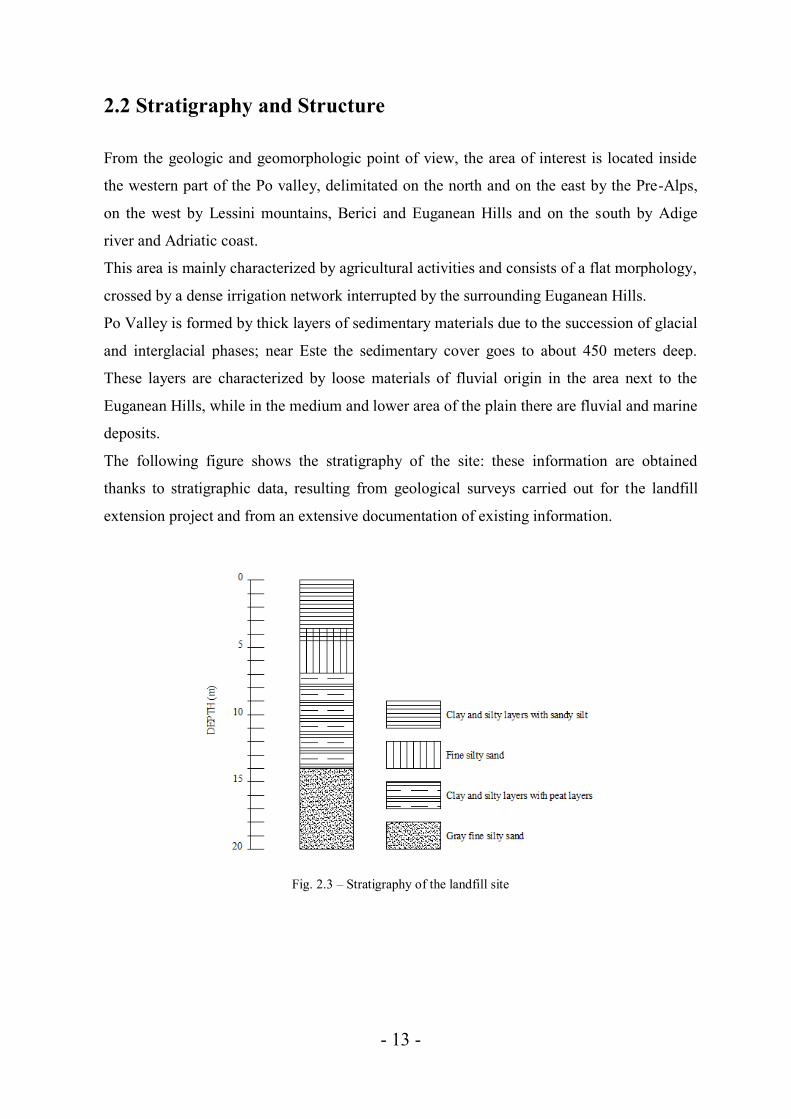
The following figure shows the stratigraphy of the site: these information are obtained

thanks to stratigraphic data, resulting from geological surveys carried out for the landfill

extension project and from an extensive documentation of existing information.

Fig. 2.3 – Stratigraphy of the landfill site

- 14 -

From the ground level to a variable depth between 3.60 and 4.50 m there is an alternation of

clay and silty layers. Inside this level there is always a sandy silt layer that starts from 0.30 –

0.80 m from the ground level having a variable thickness between 0.60 and 1.50 m.

From about 3.60 – 4.50 m to a maximum depth of 6.90 m there is a fine silty sand layer,

with a variable thickness between 0.25 and 2.40 m.

Below 6.90 m depth until about 14 m from the ground level there is a dense turnover of clay

and silty layers along with some peat layers (for a maximum thickness of 20 cm) located

between 5.0 and 8.50 m depth. These peat layers are not found in the northern part of the

landfill.

Starting from 14 m to about 20 m depth there is a gray fine silty sand layer.

It’s important to note that the average depth of the landfill is about 3-4 m depth, and the

geotechnical surveys have found a mean permeability of 10-10 m/s for the clay and silty

samples of the first layer starting from the ground surface, while previous studies have found

a permeability of about 2.3 x 10-9 – 1.24 x 10-10 m/s for these materials. These values are

conform to the guidelines of the Allegato 1 of the Legislative Decree 36/2003 that indicates

a minimum permeability value of 1 x 10-9 m/s for natural materials utilized as substratum for

non hazardous waste landfill; the prerogative of a natural barrier system having a thickness

higher or equal to 1 m is also respected.

2.3 Hydrological properties

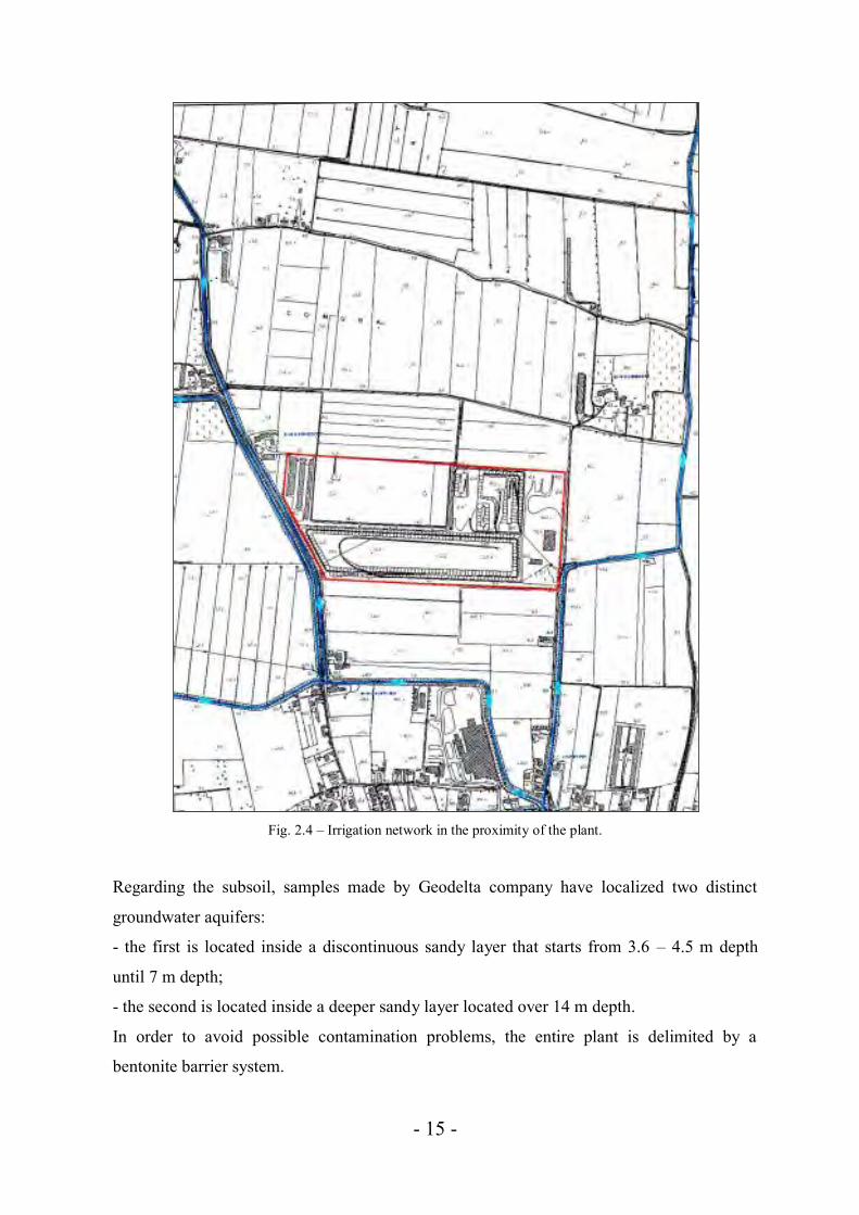
The territory surrounding the plant presents a flat morphology and is crossed by numerous

canals and drains (Fig. 2.4) connected to the local irrigation network.

Brancaglia canal flows 800 m to the east of the landfill, but in the immediate proximity are

present the following dykes: “Scolo delle Monache” (250 m from the south east side of the

landfill), “Scolo Meggiotto” (near to the west side) and “Scolo Maceratoi” (20 m from the

previous dyke), all with a thickness not superior to 4 meters and with a depth between 3 and

5 meters from the ground surface. There also small ditches (50 – 80 cm of depth) along the

north and south side of the plant.

- 15 -

Fig. 2.4 – Irrigation network in the proximity of the plant.

Regarding the subsoil, samples made by Geodelta company have localized two distinct

groundwater aquifers:

- the first is located inside a discontinuous sandy layer that starts from 3.6 – 4.5 m depth

until 7 m depth;

- the second is located inside a deeper sandy layer located over 14 m depth.

In order to avoid possible contamination problems, the entire plant is delimited by a

bentonite barrier system.

- 16 -

2.4 Climate of the site

The climate of the site belongs to the Mediterranean category with continental

characteristics, alternating cold winters to hot humid summers.

The rainfall is not too much elevate and is between 600-800 mm/year. The rainfall

distribution is a bimodal type, with an absolute maximum during spring season (May) and a

relative maximum during autumn season (October); the absolute minimum is in general in

January and the relative minimum in August.

Fig. 2.5 shows the average monthly rainfall for Este during the last 30 years.

Fig. 2.5 – Este’s average monthly rainfall (mm) for the last 30 years (Source: P.A.T.I.)

The trend of the average temperatures presents a peak in July and minimum in January (Fig.

2.6). The maximum temperatures exceed the 29 °C, a situation typical for a continental

climate with weak circulation, while the minimum temperatures are around the - 2 °C.

- 17 -

Fig. 2.6 – Este’s average monthly temperature for the last 30 years (Source: Vicenza weather station)

2.5 Seismology

Earthquake hazard can lead to a lot of problematic consequences for the landfill

management systems (like damages to barrier and cover systems and to leachate and biogas

extraction pipes) but also the stability can results very modified after a seismic event, as

happens to Chiquita Canyon landfill in California, where the Northridge earthquake of 17

January 1994 with a magnitude of 6.7 caused a progressive landslide of the lateral sides

(Matasovic et al., 1998).

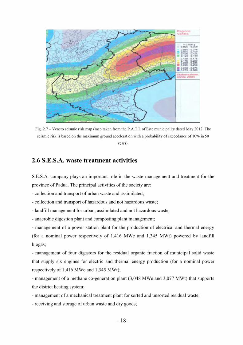
With reference to the P.A.T.I. (Piano di Assetto del Territorio Intercomunale), which is a

municipal plan for the disposition of the neighboring municipalities, Este is considered as a

part of Veneto region with low seismic risk (class 4). Regarding the Ordinance of the

President of the Council of Ministers (O.P.C.M.) 3519/96 and 3519/06, twelve new areas of

seismic hazard are been classified (Fig. 2.7): Este is classified with a peak ground

acceleration between 0.050 and 0.075 g, a very low range if compared with others belonging

to the Veneto region.

In Italy there is a specific legislation relative to the landfill construction criteria and in this

study the seismic hazard as be considered as a key factor for the slope stability study of the

landfill.

- 18 -

Fig. 2.7 – Veneto seismic risk map (map taken from the P.A.T.I. of Este municipality dated May 2012. The

seismic risk is based on the maximum ground acceleration with a probability of exceedance of 10% in 50

years).

2.6 S.E.S.A. waste treatment activities

S.E.S.A. company plays an important role in the waste management and treatment for the

province of Padua. The principal activities of the society are:

- collection and transport of urban waste and assimilated;

- collection and transport of hazardous and not hazardous waste;

- landfill management for urban, assimilated and not hazardous waste;

- anaerobic digestion plant and composting plant management;

- management of a power station plant for the production of electrical and thermal energy

(for a nominal power respectively of 1,416 MWe and 1,345 MWt) powered by landfill

biogas;

- management of four digestors for the residual organic fraction of municipal solid waste

that supply six engines for electric and thermal energy production (for a nominal power

respectively of 1,416 MWe and 1,345 MWt);

- management of a methane co-generation plant (3,048 MWe and 3,077 MWt) that supports

the district heating system;

- management of a mechanical treatment plant for sorted and unsorted residual waste;

- receiving and storage of urban waste and dry goods;

- 19 -

- receiving and storage of hazardous waste;

- remediation of contaminate sites;

- design, construction, installation and maintenance of the plants.

Fig. 2.8 shows an aerial view of the Este S.E.S.A. plant.

Fig. 2.8 – Este S.E.S.A. waste treatment plant

- 20 -

2.7 S.E.S.A. landfill description

2.7.1 General information

The plant is a controlled landfill and was classify as a landfill of first category after

provincial legislation of 1984, where it was firstly disposed municipal solid waste (MSW)

and waste similar to municipal (RSA); then it was classified as non hazardous waste landfill

considering the Legislative Decree n. 36/2003.

The waste come from the municipalities belonging to “Bacino Padova 3”, a group of 37

neighboring municipalities of the south-east region of the province of Padua (for a total

surface of 704.3 km2 and almost 142,000 inhabitants) that is responsible for management of

separate collection system.

The entire landfill occupies a total area of 130,000 m2 for a total volume of about 1,520,000

m3; recently, it was authorized by the Province a new landfilling area (“Lotto Ovest” and

“Lotto Nord”) of 44,500 m2 that will occupy a total volume (considering also provisional

and final top cover) of about 566,000 m3.

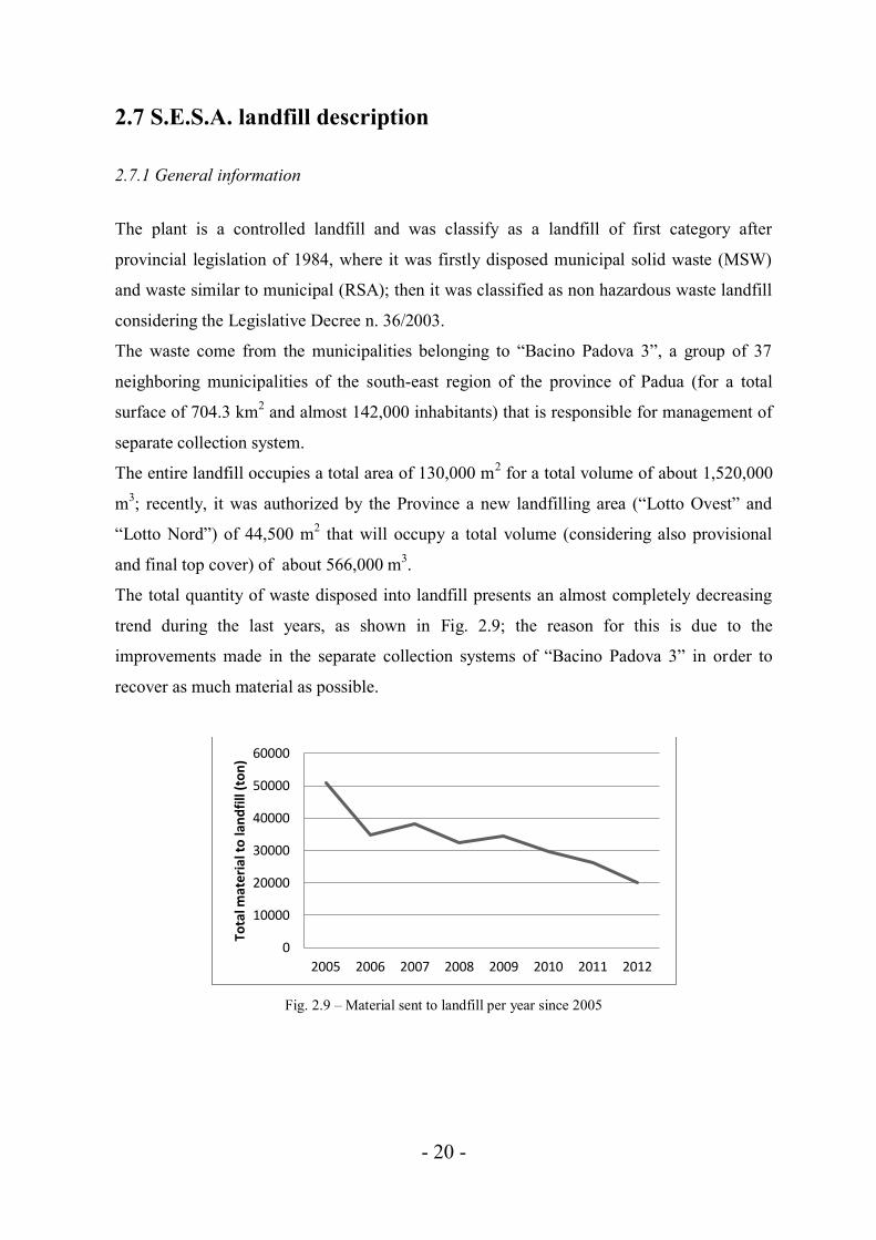
The total quantity of waste disposed into landfill presents an almost completely decreasing

trend during the last years, as shown in Fig. 2.9; the reason for this is due to the

improvements made in the separate collection systems of “Bacino Padova 3” in order to

recover as much material as possible.

Fig. 2.9 – Material sent to landfill per year since 2005

0

10000

20000

30000

40000

50000

60000

2005 2006 2007 2008 2009 2010 2011 2012

Tota

l mat

eria

l to

lan

dfi

ll (t

on

)

- 21 -

2.7.2 Principal administrative deeds

This landfill was designed in the 60s and over the years changes to the initial plan have been

made in order to increase the available volume for waste disposal maintaining also an

adequate level of safety; in this paragraph the principal authorizations and approvals

obtained over the years are presented.

The first dumping area was active since the 60s, before that S.E.S.A. company obtained the

management of the area in 1995.

Veneto Region with the Decree n.117/AMB dated 16/07/1986 and the Decree n.508 dated

22/02/1991 approved the adjustment and completion of the first dumping area named “Lotto

1”. The second dumping area named “Lotto 2” was approved by the municipality of Este

with deliberation by the council n. 56 dated 03/06/1991 and authorized by the Regional

Committee Resolution n.701 on 12 February 1992. The union of the two landfill bodies was

approved on 20 May 1997 according to the Regional Committee Resolution n.1813.

A third dumping area named “Lotto 3” (named also “Ecosistema project”) was approved by

the Veneto Committee Resolution on 17/03/1998 with deliberation n.791; an update of this

project considering also particular safety measures was approved on 16 June 2000 with

deliberation n.1696.

The management of a power plant for production of electrical and thermal energy powered

by the landfill biogas and the authorization for the installation and exercise of another power

plant for production of electrical and thermal energy powered by the biogas produced by the

anaerobic digestion plant of the organic fraction of the MSW was authorized by the

Regional Committee Resolution n.3032 dated 10/10/2003.

The plan for another enlargement of the dumping area (95,000 m3) named “Ampliamento

Lotto 3” was approved by the Province of Padua with the Measure n.4941/EC/2004 dated 30

December 2004 according to the Legislative Decree n.36/2003; S.E.S.A. company obtained

the authorization for the disposal of MSW, waste similar to municipal and non hazardous

semi-solid sludge on 8 August 2005 with the Measure of the Padua Province

n.4999/EC/2005 according to Leg. Decrees n.36/2003 and n.22/97 Art.28 and to Regional

Law n.3/2000 Art.26. Recently some new dumping areas (“Lotto Ovest” and “Lotto Nord”)

were authorized for the exercise but nowadays have not yet been realized.

- 22 -

S.E.S.A. landfill obtained also the Italian reference for the Integrated Pollution Prevention

and Control named “Autorizzazione Integrata Ambientale” (A.I.A.) with the Measure of the

Padua Province n.60/IPPC/2008 that was subsequently updated until 2018.

The entire plant received also specific environmental quality certifications like the UNI EN

ISO 14001 in the 2004 and the UNI EN ISO 9001 in the 2008.

2.7.3 Sectors and subsectors

The entire existing landfill site occupies a total surface of 130,000 m2 for a total volume of

1,520,300 m3. A new dumping area of 44,500 m2 located in the western and northern part of

the landfill has been projected and authorized but not yet realized: Fig. 2.10 shows an aerial

view of the landfill site (black line delimits the existing landfill site while red line delimits

the designed dumping area).

Fig. 2.10 – Aerial view of the existing (black line) and designed (red line) landfill site

The evolution of the landfill site started from the 60s with the first dumping area now named

as “Lotto 1”. In the 90s has been authorized and realized the second large landfill zone

- 23 -

named “Lotto 2” and then during the 2000s also “Lotto 3” has been realized. “Lotto Ovest”

and “Lotto Nord” are the last two main sites authorized for the landfilling (Fig. 2.11).

Fig. 2.11 – Scheme of the landfill dumping areas

In this paragraph the principal data of sectors and relative subsectors are described. Table

2.1 reassumes the main data (surfaces and volumes).

LOTTO 1: the first dumping site was active from the ’60 until the 1995, when S.E.S.A.

company obtained the control of the zone. This area has a trapezoidal shape for

a total surface of 72,000 m2 for a volume of about 750,000 m3.

LOTTO 2: the project for the extension of the landfill site was prepared by Este municipality

in January 1991 basing on geological and hydro- geological surveys. This site

has a rectangular shape for a total surface of about 32,000 m2 and 251,000 m3

of volume and is located in the northeastern part of “Lotto 1”; it’s subdivided

- 24 -

in 3 subsectors (S.1, S.2 and S.3), each of them subdivided in 4 basins (“Vasca

A, B, C, D”) as shown in Fig. 2.12.

The works for the realization of the sectors started in August 1995 and finished

in October 1998. The unification of “Lotto 1” with “Lotto 2” was authorized by

the Regional Committee Resolution in 1997 with an increase of volume equal

to 69,300 m3.

Fig. 2.12 – Scheme of sectors and subsectors of “Lotto 2”

LOTTO 3: the project of this rectangular area placed at the left part of “Lotto 2” was also

named “Progetto Ecosistema” and considered a new dumping site of about

20,000 m3, for a volume of 355,000 m3 taking into account also the later union

of this site with “Lotto 1”. In 2004 was design an extension of rectangular

shape named “Ampliamento Lotto 3” of about 6,000 m2 and 95,000 m3 as

volume, considering the waste settlement and the lost of mass due to the biogas

production.

“Lotto 3” is subdivided into two main sectors (S.1 and S.2) composed by other

two basins (“Vasca A,B”); also “Ampliamento Lotto 3” is formed by two

distinct basins named “Vasca A” and “Vasca B” (Fig. 2.13).

- 25 -

Fig. 2.13 – Scheme of sectors and subsectors of “Lotto 3” and “Ampliamento Lotto 3”

LOTTO OVEST: this rectangular shape site (named also “Settore 1” of the new dumping

site) has been projected but not yet realized, it will occupy an area of

about 10,500 m2 located in the north-western part of the landfill (at the

left side of “Ampliamento Lotto 3”).

LOTTO NORD: this new configuration will include a new rectangular shape area of about

34,000 m2 as surface, subdivided into three sectors (“Settore 2,3,4”)

located in the northern part of the existing landfill. The total volume of

“Lotto Ovest” and “Lotto Nord” will be equal to about 566,000 m3,

considering also the daily and final top cover materials.

Table 2.1. Principal data of the S.E.S.A. landfill sites (* = authorized but not yet realized).

SURFACE (m2)

VOLUME (m3)

LOTTO 1 72,000 750,000 LOTTO 2 32,000 251,000

Unif. L1 - L2 69,300 LOTTO 3 20,000

355,000 Unif. L1 - L3 AMPL. L3 6,000 95,000 LOTTO* OVEST 10,500

566,000 LOTTO* NORD 34,000

- 26 -

2.7.4 Bottom liner systems

S.E.S.A. landfill presents different bottom liner systems because of the development over

the years of the legislation regarding this particular aspect. For example “Lotto 1”, the part

of landfill that was active since the 60s (i.e. when a specific legislation that regulates the

entire landfill management was completely absent) doesn’t present any type of artificial

impermeabilization layer; nonetheless, as specified by the study of the stratigraphy of the

site, the natural clay layer at the bottom of the landfill could guarantee a minimum control of

leachate.

“Lotto 2”, “Lotto 3” were completed under the S.E.S.A. management and present the same

type of bottom liner system (Fig. 2.14). “Lotto Ovest” and “Lotto Nord” will have a similar

barrier system.

Fig. 2.14 – Scheme of “Lotto 2”,”Lotto 3” barrier system

2.7.5 Top cover systems

Similar to the various bottom liner systems, also the final top cover systems present some

differences relatively to the dumping sites of the landfill due to the different legislation

constraints that had to be respected over the years. The following figures show these

differences among the distinct landfill zones.

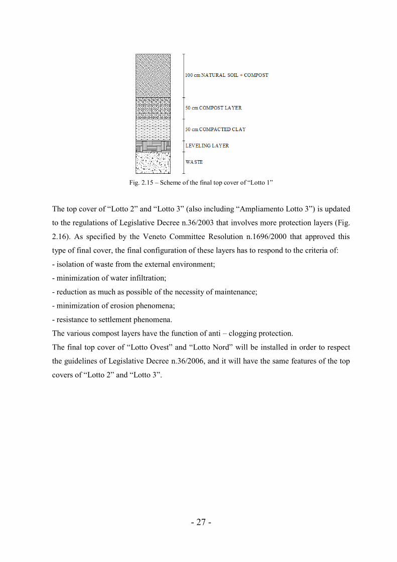
Leveling layer (in Italian “Strato di regolarizzazione”) is a particular stratus that permits the

correct installation of the overlying strata and can be composed by excavation soil, compost

or remediation soil but it has to respect particular concentrations according to CER 170504.

- 27 -

Fig. 2.15 – Scheme of the final top cover of “Lotto 1”

The top cover of “Lotto 2” and “Lotto 3” (also including “Ampliamento Lotto 3”) is updated

to the regulations of Legislative Decree n.36/2003 that involves more protection layers (Fig.

2.16). As specified by the Veneto Committee Resolution n.1696/2000 that approved this

type of final cover, the final configuration of these layers has to respond to the criteria of:

- isolation of waste from the external environment;

- minimization of water infiltration;

- reduction as much as possible of the necessity of maintenance;

- minimization of erosion phenomena;

- resistance to settlement phenomena.

The various compost layers have the function of anti – clogging protection.

The final top cover of “Lotto Ovest” and “Lotto Nord” will be installed in order to respect

the guidelines of Legislative Decree n.36/2006, and it will have the same features of the top

covers of “Lotto 2” and “Lotto 3”.

- 28 -

Fig. 2.16 – Final top cover of “Lotto 2” ,“Lotto 3”, “Lotto Ovest” and “Lotto Nord”

2.7.6 Biogas management

Starting from the 1997 drilling operations and wells installation were realized in order to

extract the biogas from the landfill along with the realization of a co-generation plant for the

energy recovery. The gas is constantly sucked by an aspirator and then conveyed to the co-

generator. A part of the produced energy is used for the maintenance of the plant while the

other remaining quantity is sell to the ENEL company.

The extraction and collection biogas system is a kind of the so-called vertical-horizontal,

where the wells are the vertical elements made in HDPE and the HDPE pipes that connect

each well to the control station are the horizontal transport elements. The control station

monitors all the pipes belonging to a certain landfill area managing the depression with

specific control valves.

From the different control stations the main pipe is connected to the co-generation plant

(Fig. 2.17) that is formed by an engine that produces electrical and thermal energy with a

nominal power of 1.41 kWh.

- 29 -

Fig. 2.17 – Co-generation plant GE Jenbacher supplied by landfill biogas

The thermal energy produced, along with the energy derived from the anaerobic digestion

systems, is sent to a district heating network that is able to supply particular public services

like the primary and secondary schools, the library and the municipal building of

Ospedaletto Euganeo and two schools and the civil hospital of Este.

The quantities of biogas extracted over the last seven years are listed in Table 2.2.

Table 2.2. Quantities of biogas extracted from the landfill per year since 2006.

Year Extracted biogas (Nm3)

2006 1,784,501.44

2007 6,573,811.39

2008 4,821,830

2009 4,601,020.5

2010 4,303,262.2

2011 3,172,361.4

2012 1,747,621.1

The constant decreasing quantity of the extracted biogas can be explained as a consequence

of the lower discharge of waste into the landfill during time, considering also that the

biodegradable quantities are less than in the past due to the improved separate collection

system and technologies that utilized this waste fraction (for example the anaerobic

digestion for the putrescible organic fraction).

- 30 -

2.7.7 Leachate management

The leachate management system is formed by 35 extraction wells, HDPE pipes that

constitute the conveying network, two inox steel storage tanks for a total capacity of 50 m3

and a control station for the monitoring. Over the years there have been upgrading and

adjustment operations were made in order to improve the catchment network.

The blowdown of the wells occurs with submergible pumps connected to the external

storage tanks, maintaining always a low hydraulic head inside the wells; leachate is then

taken with tankers by the S.E.S.A. operators and sent to the Este’s wastewater treatment

plant or to the internal physical-chemical plant reducing transportation costs and also

environmental impact.

The leachate analysis is made every three months with the samples taken from the adduction

pipes of the different landfill sectors connected to the storage tanks; another analysis on the

leachate sampled directly from the storage tanks is made once a year.

The drainage network (that will be the same also for the new projected sectors) is formed by

HDPE corrugated pipes with saw teeth profile with an external diameter of 200 mm and an

internal diameter of 171 mm. The network is placed inside a wasp nest gravel that has a

thickness in the higher point equal to 60 cm.

The landfill bottom presents a double inclination of one degree and each sector is divided by

anchor trenches of trapezoidal section in order to favor the leachate drainage. The drainage

pipes of each sector are connected to two external concrete wells where electrical

submergible pumps are installed. The pumps are linked to the storage tanks with HDPE DN

75 pipes.

The quantity of the extracted leachate over the last seven years is shown in Table 2.3.

Table 2.3. Leachate extracted since 2006.

Year Extracted leachate (ton)

2006 10,779.94

2007 12,549.3

2008 11,294.71 2009 9,990.74

2010 11,076.65

2011 7,095.04

2012 12,968.97

- 31 -

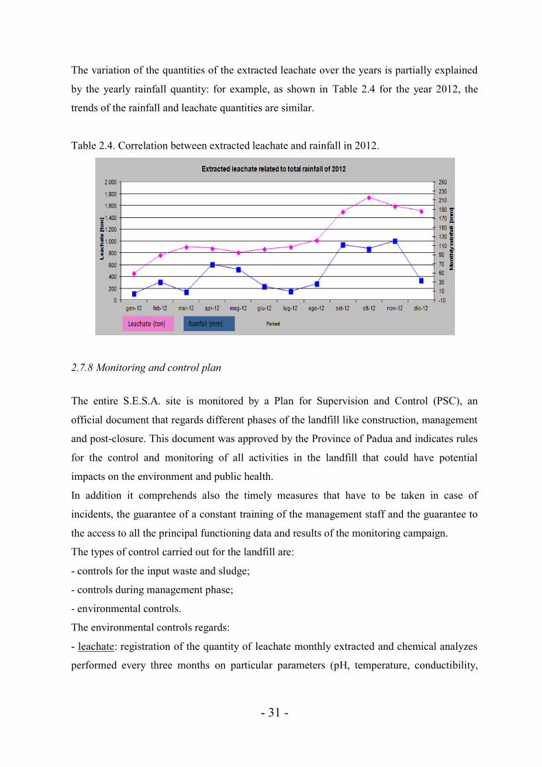
The variation of the quantities of the extracted leachate over the years is partially explained

by the yearly rainfall quantity: for example, as shown in Table 2.4 for the year 2012, the

trends of the rainfall and leachate quantities are similar.

Table 2.4. Correlation between extracted leachate and rainfall in 2012.

2.7.8 Monitoring and control plan

The entire S.E.S.A. site is monitored by a Plan for Supervision and Control (PSC), an

official document that regards different phases of the landfill like construction, management

and post-closure. This document was approved by the Province of Padua and indicates rules

for the control and monitoring of all activities in the landfill that could have potential

impacts on the environment and public health.

In addition it comprehends also the timely measures that have to be taken in case of

incidents, the guarantee of a constant training of the management staff and the guarantee to

the access to all the principal functioning data and results of the monitoring campaign.

The types of control carried out for the landfill are:

- controls for the input waste and sludge;

- controls during management phase;

- environmental controls.

The environmental controls regards:

- leachate: registration of the quantity of leachate monthly extracted and chemical analyzes

performed every three months on particular parameters (pH, temperature, conductibility,

- 32 -

ammonia nitrogen, nitrates, nitrites, chlorides, sulfate, metals, iron and manganese. Every

year the analyzes regards also other parameter such as COD and hydrocarbons;

- biogas: monthly evaluation of the parameters of methane, oxygen and carbon dioxide;

- surface water: annual analysis on particular parameters in the surrounding draws. The

monitoring regards: temperature, pH, conductivity, COD, BOD5, ammonia nitrogen,

nitrates, nitrites, chlorides, sulfate, metals, organohalogen compounds, pesticides, solvents,

hydrocarbons;

- groundwater: ten control wells are installed for the monthly measurement of the levels of

the shallow and deep aquifers. Every three months controls are performed to evaluate

temperature, pH, conductibility, permanganate oxidability, ammonia nitrogen, nitrates,

nitrites, chlorides, sulfate, metals, iron and manganese. Every year the analyzes is extended

to other parameters like BOD5 and PAH;

- air quality: two points for semiannual examination of hydrogen sulfide and ammonia and

for annual examination of dusts;

- weather-climate parameters: daily measurements of precipitations, temperature, wind

direction and intensity and atmospheric humidity;

- landfill morphology: semiannual examination of volume occupied by waste and available

volume for the disposal;

- external noise: annual phonometric investigation on the perimeter of the site.

- 33 -

3. General slope stability concepts

3.1 Introduction

One of the most critical aspects that an engineer must take into account during the design

and the management of a landfill is the space saving: this is not only a question of

sustainability with ecological footprint consideration, but it’s also a delicate issue due to the

numerous administrative permits to obtain in order to respect different constraints like the

proximity to residential areas or sensitive natural sites.

This aspect can be solved with a reduction of the dimension of the incoming waste to the

landfill, for example through compaction of compressible waste, but also diminishing the

ratio between horizontal and vertical dimension of the landfill with the result of a higher and

inclined structure along the slopes.

To implement this second procedure the elaboration of a stability analysis is fundamental,

not only during the project phase, but also during the operational and post operational period

because some particular waste can change their properties during time (because of

degradation processes and changes of unit weight) leading for example to different shear

strength parameters and pore water pressure, i.e. two of the most critical characteristics for

the stability.

Moreover, the issue of slope stability is crucial for other reasons: the safety of on-site

workers, the protection of investments made in improving the level of engineering of the

landfill (like the biogas collection system) and the prevention of large remediation costs

(Gharabaghi et al., 2007). Also the introduction of geosynthetic materials through the liner

systems has increase the attention to this study due to the carefulness that has to be paid to

the integrity of the liners during time.

The study of this problem is very complex due to the heterogeneity of waste and to the

ability to obtain geotechnical parameters such as density, moisture content, friction angle

and cohesion; laboratory measures present limitations not only for the heterogeneous nature

of MSW, but also for the erratically changing of properties within the landfill during time

(Vajirkal, 2000).

- 34 -

Usually, literature data indicate the cone penetrometer test as the most accurate procedure to

obtain these particular waste parameters, thanks to the high accuracy and minimal efforts

and costs of this device that it’s able to characterize a large area in a short time period

(Vajirkar, 2000).

There are two different types of calculation to study the slope stability analysis: the Limit

Equilibrium Methods (LEM) and the Finite Element Methods (FEM); the main difference is

that the LEM are based on the static of equilibrium while the FEM are related to the stress –

strain relationship.

Both methods will be discussed on this thesis and the Este’s S.E.S.A. landfill slope stability

will be evaluated using two different calculation softwares that represent these analyses

approaches: SLOPE/W for the LEM and PLAXIS for the FEM.

3.2 Factors of influence

Instability of landfills results in most cases as a combination of gravitational forces and

water pressures; when gravitational forces are out of balance the failure occurs. Water plays

the role of lubricant diminishing the resisting forces causing gradually an increasing of

sliding mass velocity that finally leading to the failure. Gravitational forces and water are

two of the main causes of the instability. This paragraph presents a briefly description for

the factors of influence of the stability ([27],[38],[39],[40]) excluding the seismic

contribution that will be discussed further in more detail.

Landfill geometry

The main factors that influence the stability are those which characterize the geometry such

as height and angles of side slopes of the landfill. In order to maintain stability is important

that bottom, top cover and side slope liners are designed as flat as possible, because

instability might occur if the projected slopes were steeper than the friction angle between

the materials; the erosion can be limited with a soil vegetation layer in the top cover.

Shear strength

- 35 -

This factor is crucial for the stability because characterizes the interaction between different

materials such as geosynthetic liners and soil; moreover, also the strength characteristics of

waste are important because moisture content and organic waste (for co-disposal landfill

cases) can determine a reduction in the stability.

Unit weight of waste

This parameter is essential because gives an idea of the compressibility of the waste mass;

unfortunately, there are significant uncertainties regarding its value. It’s very difficult to

obtain a certain value, because unit weight values vary significantly not only among

different sites but also within the same site.

Compaction effort, layer thickness, overburden stress, moisture content, variations in waste

constituents (like size and density), state of decomposition and degree of control during

placement (like thickness of daily cover) are the factors that influence unit weight of waste.

A study conducted by Zekkos et al. (2006) proposed an hyperbolic function to describe the

relationship between MSW unit weight and depth.

Water content and pore water pressure

Water content of landfill can change due to several factors like waste composition, time of

year, rising groundwater accumulation and meteorological conditions. Seepage forces may

reduce the resisting forces along the failure surface increasing the driving forces.

Pore pressure can be influenced also by leachate and co-disposal of biosolids. This can lead

to an increase of MSW unit weight decreasing the effective stress which eventually lead to

shear strength reduction affecting the landfill stability. For the opposite reason a diminishing

of the pore water pressure lead to an increase of effective vertical stress making the landfill

more stable.

Settlement

Shafer (2000) proposed two different types of settlement that affect landfill stability. One is

related to the uniform settlement that, thanks to densification, increase the unit weight of

waste favoring the stability; the other one is the localized differential settlement that

- 36 -

promotes surface water to infiltrate within the mass, potentially increasing pore water

pressure and piezometric head in the waste mass. This second type of settlement can be

related to the presence of biosolids which have high compressibility creating local

settlement zones which have a negative consequence for the stability.

External loadings

External loads such as daily top cover, final cover, the movement of vehicles, traffic and

stockpiles of materials can affect the landfill stability.

Landfill management

Some particular operations can be done in order to improve landfill stability, such as the mix

of biosolids with MSW before landfilling. Also other landfill management systems like

biogas and leachate extraction wells should be monitored regularly in order to prevent any

damage to the barrier layers.

Vegetation

Vegetation is important not only for aesthetic reasons but also for its property against

erosion processes; moreover, vegetation on landfill slopes improves the slope stability

because the vegetation roots add cohesion to the top soil acting as a reinforcement.

3.3 Types of landfill’s failure

Landfill slope failures are usually due to the loss of shear strength by the multilayer

composites, to a change in geometrical properties such as the steepening of an existing slope

or to an excessive settlement of waste. The typical geotechnical failure types are also

possible depending on site-specific conditions (like the type of cover used) and the

placement and geometry of the MSW mass.

In this paragraph potential failure modes are briefly described. Figures are taken from

“Geotechnical aspects of landfill design and construction” by X. Quian, R.M. Koerner, D.H.

Gray.

- 37 -

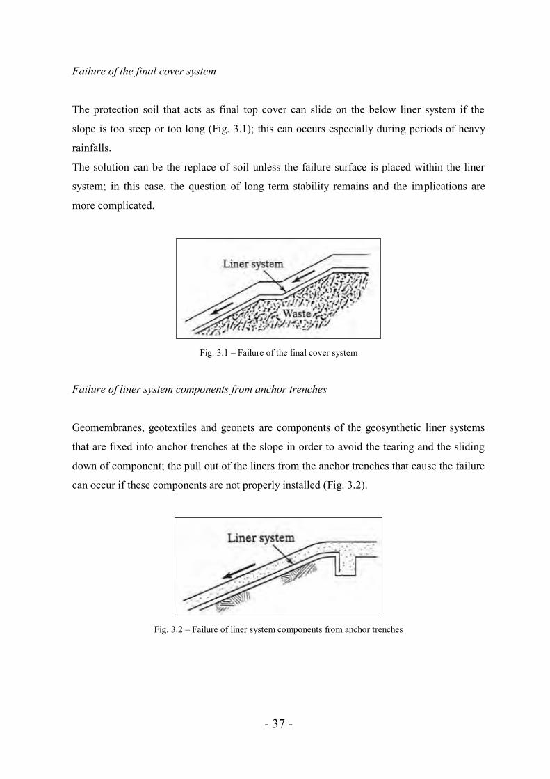
Failure of the final cover system

The protection soil that acts as final top cover can slide on the below liner system if the

slope is too steep or too long (Fig. 3.1); this can occurs especially during periods of heavy

rainfalls.

The solution can be the replace of soil unless the failure surface is placed within the liner

system; in this case, the question of long term stability remains and the implications are

more complicated.

Fig. 3.1 – Failure of the final cover system

Failure of liner system components from anchor trenches

Geomembranes, geotextiles and geonets are components of the geosynthetic liner systems

that are fixed into anchor trenches at the slope in order to avoid the tearing and the sliding

down of component; the pull out of the liners from the anchor trenches that cause the failure

can occur if these components are not properly installed (Fig. 3.2).

Fig. 3.2 – Failure of liner system components from anchor trenches

- 38 -

Rotational failure within the waste mass

This type of failure is completely independent of the liner system (Fig. 3.3): it involves a

movement of a large amount of material from the circular failure surface located within the

waste body to the toe of the slope. The reasons of this instability are a too steep waste slope,

high liquid content or lack of waste placement control.

Fig. 3.3 – Rotational failure within the waste mass

Rotational failure through waste mass, liner and foundation soil

Failure can starts from the bottom soft soil propagating until the waste mass; the failure

plane may be at or within the liner system, or in the soft subsoil (Fig. 3.4). One reason can

be the excessive waste weight. These types of instability have occurred in both unlined and

lined sites involving up to 500,000 m3 of waste.

Fig. 3.4 – Rotational failure through waste mass, liner and foundation soil

Rotational failure of soil slope, toe or base

The soil mass behind the waste body or beneath the site could presents instability and then

failing. The failure occurs along the slope, at the toe or within the foundation soil (Fig. 3.5).

- 39 -

The reasons can be a too steep slope or the soft foundation soil properties, not involving

liner system or waste properties like shear strength or unit weight.

Fig. 3.5 - Rotational failure of soil slope, toe or base

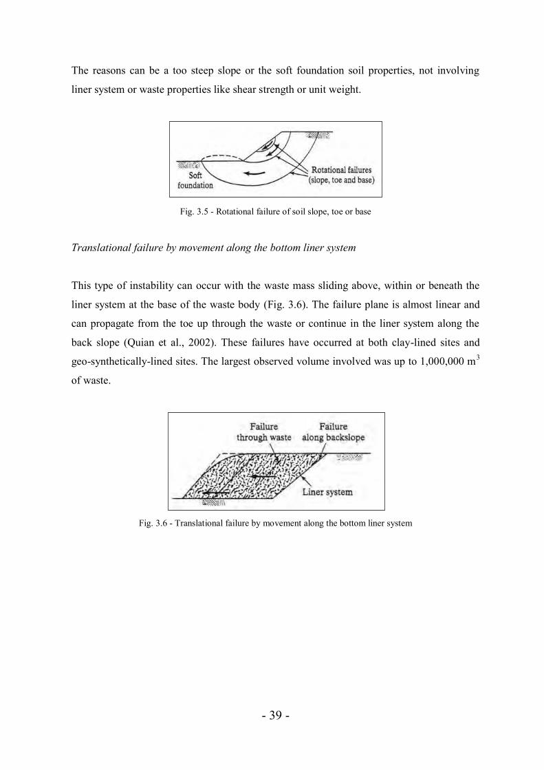
Translational failure by movement along the bottom liner system

This type of instability can occur with the waste mass sliding above, within or beneath the

liner system at the base of the waste body (Fig. 3.6). The failure plane is almost linear and

can propagate from the toe up through the waste or continue in the liner system along the

back slope (Quian et al., 2002). These failures have occurred at both clay-lined sites and

geo-synthetically-lined sites. The largest observed volume involved was up to 1,000,000 m3

of waste.

Fig. 3.6 - Translational failure by movement along the bottom liner system

- 40 -

3.4 Seismic contribution

The seismic or dynamic forces are usually oscillatory, multi-directional and act only for

moments in time; in order to represent the dynamic loading the static forces are usually

involved in this type of study. After the shaking the slope may not completely collapse, but

there may be some unacceptable permanent deformations.

As required also by Italian Legislation, a pseudostatic analysis can be performed to consider

the dynamic effects, describing the effects of earthquake shaking by accelerations that create

inertial forces which act in the horizontal and vertical directions at the centroid of each slice.

This type of analysis is a sort of extension of the limit equilibrium method with the addiction

of the component of inertia that represents the action of the seismic effect. Seismic

contribution is considered introducing static forces applied to the center of gravity of the

mass potentially sliding and proportional to the weight W of the interested mass (Fig. 3.7).

Fig. 3.7 – Inertial forces of the seismic contribution

These forces are defined as:

where:

- W = slice weight;

- = coefficient of the maximum acceleration reduction;

- 41 -

- = maximum seismic acceleration estimated for the site of interest;

- g = gravity acceleration (9.81 m/s2);

The value of is defined basing on the stratigraphic (stratigraphic coefficient Ss) and

topographic (topographic coefficient ST) situation:

The coefficient ag represents the maximum horizontal acceleration for the site of interest

considering hard ground soil (“A” type for subsoil categories).

Referring to the NTC08 for the Italian legislation, all these coefficients can be found in

order to set the values of KH and KV to the computer programs.

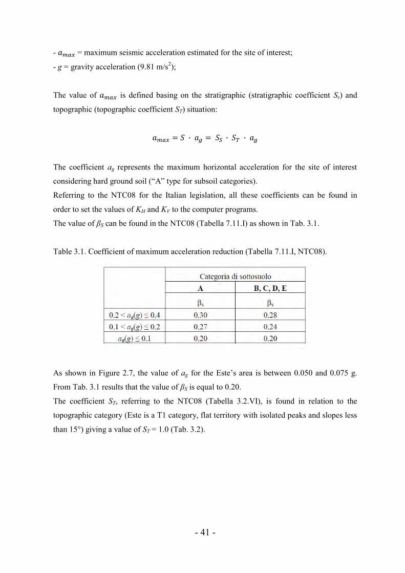
The value of βS can be found in the NTC08 (Tabella 7.11.I) as shown in Tab. 3.1.

Table 3.1. Coefficient of maximum acceleration reduction (Tabella 7.11.I, NTC08).

As shown in Figure 2.7, the value of ag for the Este’s area is between 0.050 and 0.075 g.

From Tab. 3.1 results that the value of βS is equal to 0.20.

The coefficient ST, referring to the NTC08 (Tabella 3.2.VI), is found in relation to the

topographic category (Este is a T1 category, flat territory with isolated peaks and slopes less

than 15°) giving a value of ST = 1.0 (Tab. 3.2).

- 42 -

Table 3.2. Topographic coefficients (Tabella 3.2 VI, NTC08).

To find the value of Ss is firstly necessary to define the value of another coefficient F0 that

from the Appendixes of NTC08 is taken equal to 2.49 (basing on latitude and longitude of

the site), and considering a C type (“Tabella 3.2 II” of NTC08) for SESA landfill subsoil

category (deposits of coarse grained soils with medium thickness or fine grained soils with a

medium consistency), the following formula gives a value for the Ss coefficient:

The calculation gives a results higher than 1.5; in this case, the value that has to be

considered is SS = 1.5.

Now it’s possible to define amax, KH and KV:

= 1.5 ∙ 1.0 ∙ 0.075 = 0.1125 g

The two last values will be inserted in the two calculation softwares.

- 43 -

4. Slope Stability Analysis methods

4.1 Introduction

Slope stability analysis is carried out in order to evaluate the safe design of natural (where

instability is usually due to the erosion) or artificial slopes (generated by cuttings,

excavations or building of embankments) and the conditions for the equilibrium: generally,

instability is the result of a combination of gravitational forces and water pressures, usually

the main causes of the failure mechanisms.

The main purpose of this type of study is the identification of endangered areas establishing

a factor of safety for the potential slip surfaces considering factors as safety, reliability and

economics in the long period establishing also potential remedial measures for the most

critical cases.

Before the introduction of powerful personal computers, stability analysis was performed

graphically or using hand-calculations; simplifying hypothesis had to be taken to find

solutions, and the concept of numerically dividing a larger soil body into smaller parts was

the most adopted simplification.

Nowadays geotechnical engineers have a lot of possibilities thanks to the use of computer

software products that permit to deal with a lot of variables like complex stratigraphy, highly

irregular pore-water pressure conditions, almost any type of slip surface shape, concentrated

and distributed loads and different linear and nonlinear shear strength models.

The software possibilities ranges from limit equilibrium techniques through finite element

limit approaches, and as easily predictable each methods presents its pros and cons: for

example, limit equilibrium is the most commonly used and presents simple solution

techniques, but it can results unsuitable if the slope fails by complex mechanisms (like

internal deformations, progressive creep, etc.).

During the last decade new applications are been developed as the Slope Stability Radar, a

system to remotely scan a rock slope to control the spatial deformations of the face,

detecting small movements with sub-millimeter accuracy by using interferometry

techniques.

- 44 -

4.2 General concepts of Limit Equilibrium Methods

The study of the stability of the earth structures is the oldest type of numerical analysis in

geotechnical engineering (SLOPE/W tutorial manual). The first studies were introduced

early in the 20th Century: in 1916 Patterson presented a stability analysis of the Stigberg

Quay in Gothenberg (Sweden), where the first idea of dividing a potential failure mass into

slices was proposed. One of the reasons the limit equilibrium approach was adopted so

quickly is that solutions could be founded by hand-calculations.

During the next few decades this study was developed and improved by other engineers like

Fellenius and Janbu, until the 1960’s when the coming of electronic computers led this

technique to more rigorous formulations such as those elaborated by Morgenstern and Price

and by Spencer.

All these methods are similar each other but they are also different due to the hypotheses

made; nevertheless, there are some general hypotheses that are common to all the limit

equilibrium methods (Favaretti):

1 - Mohr-Coulomb failure criterion is satisfied along the hypothetical failure surface, which

may be a straight line, circular arc, logarithmic spiral or other irregular surface. The MC

failure criterion represents the linear envelope that is obtained from a plot of shear strength

of a material versus the applied normal stress (Fig. 4.1). The relation is expressed as:

where: is the shear strength at failure on the failure plane, is the intrinsic cohesion of the

material (and the intercept of the failure envelope), is the normal stress at failure on the

failure plane and is the angle of internal friction (and the slope of the failure envelope).

This equation can contain the pore water pressure u in cases of drained conditions (effective

stress):

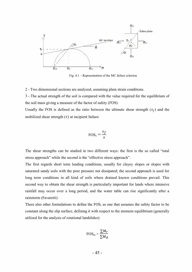
- 45 -

Fig. 4.1 – Representation of the MC failure criterion

2 - Two dimensional sections are analyzed, assuming plain strain conditions.

3 - The actual strength of the soil is compared with the value required for the equilibrium of

the soil mass giving a measure of the factor of safety (FOS).

Usually the FOS is defined as the ratio between the ultimate shear strength ( ) and the

mobilized shear strength ( at incipient failure:

FOSτ =

The shear strengths can be studied in two different ways: the first is the so called “total

stress approach” while the second is the “effective stress approach”.

The first regards short term loading conditions, usually for clayey slopes or slopes with

saturated sandy soils with the pore pressure not dissipated; the second approach is used for

long term conditions in all kind of soils where drained known conditions prevail. This

second way to obtain the shear strength is particularly important for lands where intensive

rainfall may occur over a long period, and the water table can rise significantly after a

rainstorm (Favaretti).

There also other formulations to define the FOS, as one that assumes the safety factor to be

constant along the slip surface, defining it with respect to the moment equilibrium (generally

utilized for the analysis of rotational landslides):

FOSm =

- 46 -

where is the sum of the resisting moments and is the sum of the driving moments.

The force equilibrium is generally used to translational or rotational failure that can be

composed by planar or polygonal slip surfaces:

FOSf =

where is the sum of the resisting forces and is the sum of the driving forces.

It’s important to note that the simplest slope stability analysis methods cannot fulfill both

force and moment equilibrium simultaneously and that these definitions can be very

different in the values and the meaning. Nevertheless, most design codes do not present a

clear requirement on what FOS they are referring, and only a single safety factor is specified

in many of these codes.

The instability of slopes occurs when the FOS 1.0, but in practice this is not completely

true because the failure is also caused by the velocity of the sliding soil mass; usually, until

F = 1.25 failure doesn’t occur (Favaretti, 2010).

4 - Soils are treated as rigid-plastic materials and due to this hypothesis the analysis does not

consider deformations.

Limit equilibrium methods can be subdivided in two principal categories:

methods that consider only the whole soil body (Taylor method, Culmann method);

methods that subdivide the mass into many slices (that can be vertical or non vertical

like for the Sarma’s method) considering the equilibrium of each slide (method of

slices).

In this study only the methods of slice will be presented because are those used by computer

programs and the only types of calculation methods provided for by law; moreover, methods

that considers the whole soil body are useful for slopes with homogeneous materials.

- 47 -

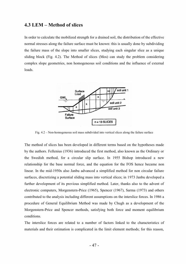
4.3 LEM – Method of slices

In order to calculate the mobilized strength for a drained soil, the distribution of the effective

normal stresses along the failure surface must be known: this is usually done by subdividing

the failure mass of the slope into smaller slices, studying each singular slice as a unique

sliding block (Fig. 4.2). The Method of slices (Mos) can study the problem considering

complex slope geometries, non homogeneous soil conditions and the influence of external

loads.

Fig. 4.2 – Non-homogeneous soil mass subdivided into vertical slices along the failure surface

The method of slices has been developed in different terms based on the hypotheses made

by the authors. Fellenius (1936) introduced the first method, also known as the Ordinary or

the Swedish method, for a circular slip surface. In 1955 Bishop introduced a new

relationship for the base normal force, and the equation for the FOS hence became non

linear. In the mid-1950s also Janbu advanced a simplified method for non circular failure

surfaces, discretizing a potential sliding mass into vertical slices; in 1973 Janbu developed a

further development of its previous simplified method. Later, thanks also to the advent of

electronic computers, Morgenstern-Price (1965), Spencer (1967), Sarma (1973) and others

contributed to the analysis including different assumptions on the interslice forces. In 1986 a

procedure of General Equilibrium Method was made by Chugh as a development of the

Morgenstern-Price and Spencer methods, satisfying both force and moment equilibrium

conditions.

The interslice forces are related to a number of factors linked to the characteristics of

materials and their estimation is complicated in the limit element methods; for this reason,

- 48 -

simplified assumptions are made in most approaches either to neglect both or one of them.

Nevertheless, the most accurate methods consider these forces in their analysis.

Anyhow, all these methods can be subdivided in three categories basing on the different

hypotheses (Favaretti, 2010):

- assumptions on interslice force direction (Bishop, Morgenstern-Price, Spencer);

- assumptions on the thrust line position (Janbu);

- assumptions on the interslice forces distribution (Sarma).

As previously discussed, other suppositions are those that tend to divide a slide mass into n

smaller slices (and so the irregular base of the slice can be approximated to a chord) and the

FOS is considered constant along the failure surface.

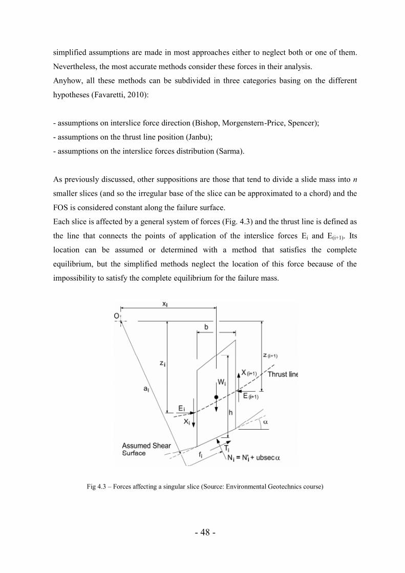
Each slice is affected by a general system of forces (Fig. 4.3) and the thrust line is defined as

the line that connects the points of application of the interslice forces Ei and E(i+1). Its

location can be assumed or determined with a method that satisfies the complete

equilibrium, but the simplified methods neglect the location of this force because of the

impossibility to satisfy the complete equilibrium for the failure mass.

Fig 4.3 – Forces affecting a singular slice (Source: Environmental Geotechnics course)

- 49 -

In fact for this system there are (6n – 2) unknowns but only four equations (4n) for each

slice can be written for the system equilibrium limit (Tab. 4.1); for this reason the solution is

statically indeterminate.

Table 4.1. Equations and unknowns of the limit equilibrium of each slice (Source:

Environmental Geotechnics course).

Considering Table 4.1, the total unknowns are:

6n – 2 – 4n = 2n -2

An assumption to reduce the unknowns number is usually to consider the normal forces on

the base of the slices acting at the midpoint; with this hypothesis the number of remaining

unknowns becomes:

5n – 2 – 4n = n – 2

These are the general assumptions that characterized the available methods of analysis that

will be discussed in the further subchapter.

- 50 -

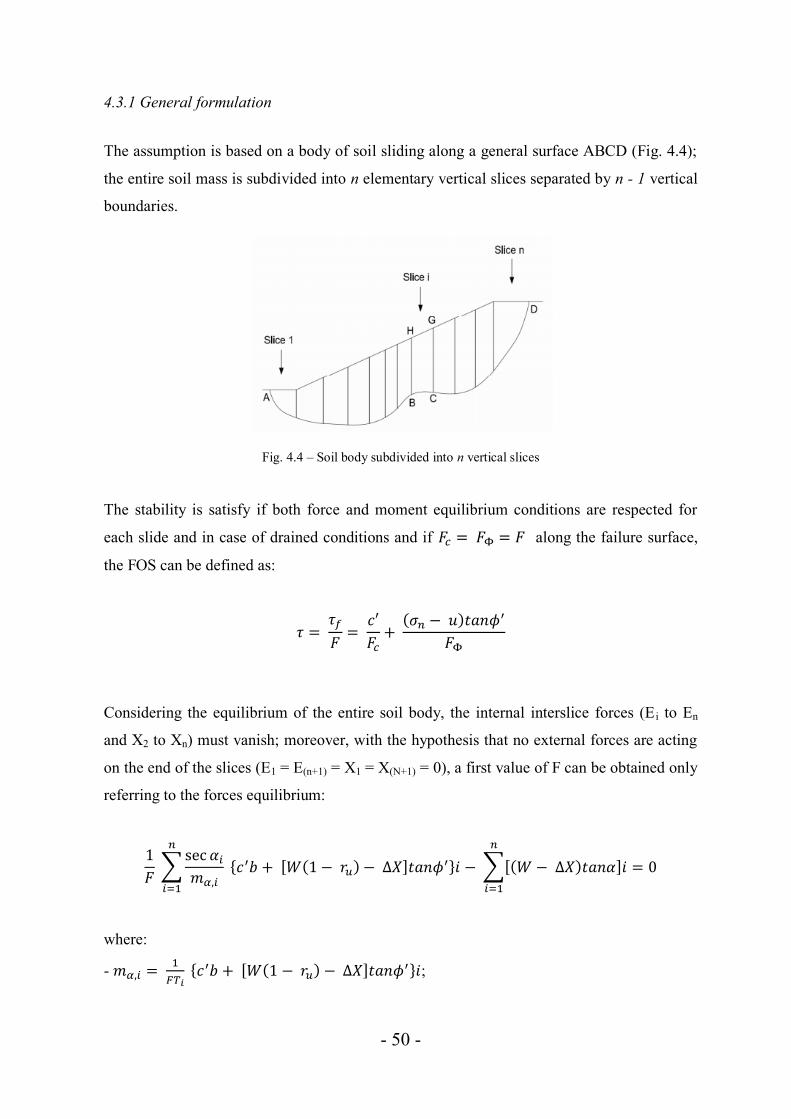
4.3.1 General formulation

The assumption is based on a body of soil sliding along a general surface ABCD (Fig. 4.4);

the entire soil mass is subdivided into n elementary vertical slices separated by n - 1 vertical

boundaries.

Fig. 4.4 – Soil body subdivided into n vertical slices

The stability is satisfy if both force and moment equilibrium conditions are respected for

each slide and in case of drained conditions and if along the failure surface,

the FOS can be defined as:

Considering the equilibrium of the entire soil body, the internal interslice forces (E i to En

and X2 to Xn) must vanish; moreover, with the hypothesis that no external forces are acting

on the end of the slices (E1 = E(n+1) = X1 = X(N+1) = 0), a first value of F can be obtained only

referring to the forces equilibrium:

where:

-

;

- 51 -

- ru = coefficient of pore water pressure =

Considering the moment equilibrium of slice i around pivot O and that the moments of all

internal forces (Ei, Xi) must vanish for the entire body, an expression for the equilibrium of

moments can be obtained:

In cases of circular failure surface (ai = R, fi = 0 and xi = Risenα) the previous equation

becomes:

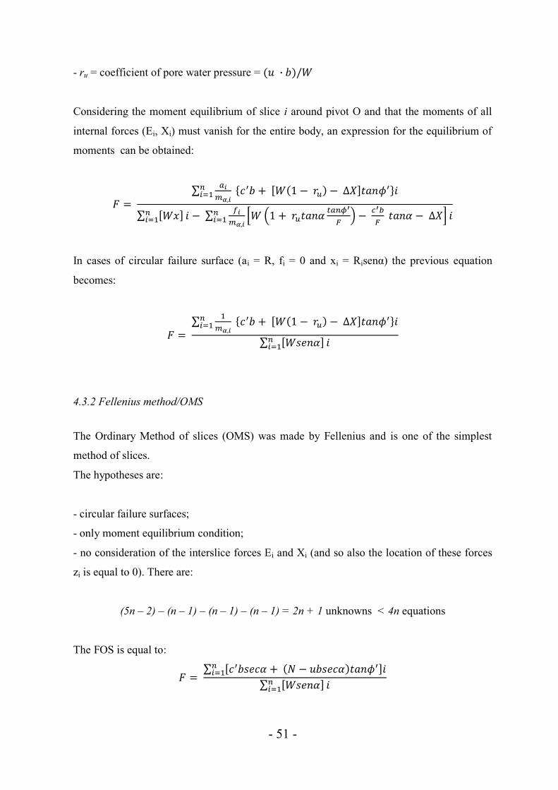
4.3.2 Fellenius method/OMS

The Ordinary Method of slices (OMS) was made by Fellenius and is one of the simplest

method of slices.

The hypotheses are:

- circular failure surfaces;

- only moment equilibrium condition;

- no consideration of the interslice forces Ei and Xi (and so also the location of these forces

zi is equal to 0). There are:

(5n – 2) – (n – 1) – (n – 1) – (n – 1) = 2n + 1 unknowns ˂ 4n equations

The FOS is equal to:

- 52 -

The advantage of this method is its simplicity in solving the FOS, since the equation does

not require an iteration process.

4.3.3 Bishop’s rigorous method

This method is very common in practice of slope stability analysis, and its assumptions are:


- both forces and moments equilibrium are satisfied;

- interslice vertical forces Xi (n – 1 unknowns) defined as: Xi = λ f(x) where λ is a constant

unknown (“+1”) and f(x) a known function. The number of unknowns and equations

become:

(5n – 2) – (n – 1) + 1 = 4n unknowns = 4n equations

In this way the problem is determinate and the equations of equilibrium are satisfied.

It’s important to note that there are several combinations between λ and f(x) that satisfy the

problem, but some of these are not possibles because there are two other aspects that have to

be respected:

- shear strength along vertical interslice surfaces must be less than the failure strength of soil

because these surfaces can’t reach the failure condition (τi = Xi/Ai ˂ τf = c’ + σ’tanϕ’);

- the thrust line must be located inside the sliding body (Fig. 4.5). A solution where the

thrust line is located externally to the soil body is not phisically acceptable.

Fig. 4.5 – Thrust line position

- 53 -

4.3.4 Bishop’s simplified method

The hypotheses of this method are:


- only moments equilibrium condition;

- neglection of the interslice vertical forces Xi. There are:

(5n – 2) – (n – 1) = 4n - 1 unknowns ˂ 4n equations

and so the problem is overdeterminated.

Considering that Xi = 0, λ = 0 and ΔXi = 0 the FOS is equal to:

The solution of the Bishop’s method can be found with an iterative procedure:

- assume an initial value of F → F0;

- calculate mα,i with F0 for each slice;

- determine F using mα,i (if F = F0 the procedure is complete, otherwise the iteration

procedure continues).

4.3.5 Janbu’s simplified method

The assumptions are:

- any type of failure surface;

- only force equilibrium condition;

- interslice vertical forces Xi = 0 (similarly to the Bishop’s simplified method) leading to an

overdeterminated solution that will not satisfy the conditions of the moment equilibrium.

The FOS is equal to:

- 54 -

In order to correct the overestimated value of the FOS, Janbu presented a correction factor f0

> 1 that has to be multiplied to the previous calculated safety factor to obtain a final value of

FOS. This correction factor is a function of the slide geometry and the strength parameters

of the soil (Fig. 4.6); in cases of surface intersecting different soil types, the curve c – ϕ is

generally used to estimate the f0 value.

Fig. 4.6 – Estimation of the corrective factor f0 (Source: Environmental Geotechnics course)

As an alternative, the corrective factor f0 can also be calculated with the following formula:

where b1 depends on the soil type:

- b1 = 0.69 for c only soils (i.e. for clayey soils);

- b1 = 0.31 for ϕ only soils (i.e. soils without cohesion);

- b1 = 0.5 for c and ϕ soils.

- 55 -

4.3.6 Janbu’s generalized method

This is an advanced procedure of Janbu’s method and the hypotheses are:

- any kind of failure surface;

- both force and moment equilibrium conditions satisfied, since it assumes a location of the

thrust line (leading to 4n – 1 unknowns) suggesting also that the actual position of the thrust

line is an additional unknown, and thus equilibrium can be respected if the assumption

selects the correct thrust line. This line is searched using an iteration procedure until the

equilibrium is reached.

4.3.7 Morgenstern – Price method

The assumptions are:


- both force and moment equilibrium conditions satisfied;

- the interslice force inclination can vary with an arbitrary function f(x) (leading the number

of unknowns equal to 4n):

where:

- λ = scale factor of the assumed function;

- f(x) = interslice force function that varies continuously along the slip surface.

4.3.8 Spencer’s method

This method derives from the previous method and satisfies static equilibrium by assuming

that the interslice force inclination can vary with a constant but unknown function f(x) =

constant.

- 56 -

4.3.9 Lowe – Karafiath’s method

The hypotheses are:


- only force equilibrium is satisfied assuming that the interslice forces are inclined at an

angle equal to the average of the slope ground surface angle β and slice base angle α; this

simplification leads to 4n – 1 unknowns failing to satisfy the moment equilibrium.

Considering θ = inclination of the interslice resultant force the two equations are:

4.3.10 Corps of Engineers method

The approach is similar to the previous one, but the assumption on the inclination of the

interslice forces θ can be done in two different types: it considers θ parallel to the slope

ground surface inclination β (i.e. θ = β) or equal to the average slope inclination between the

left and right end points of the failure surface. This hypothesis makes the problem

overdetermined and moment equilibrium is not satisfied.

4.3.11 Sarma’s method

This method is quite different from the other ones because it was implemented for non-

vertical slice or for general blocks (wedge method). It assumes a relationship for the

interslice forces similar to the Mohr-Coulomb expression:

where:

- c and ϕ are the shear strength parameters (cohesive component and material friction angle);

- 57 -

- h is the slice height.

This assumption makes the problem solvable both for force and moment equilibrium (the

interslice forces are adjusted until the FOS satisfies the two equilibrium equations).

It’s important to note that this method works best when the cohesion is zero or at least very

small: if c = 0, the interslice shear is directly proportional to the normal as with all the other

approaches.

4.3.12 General limit equilibrium formulation

The GLE formulation was studied by Fredlund at the University of Saskatchewan in the

1970s (Fredlund and Krahn 1977; Fredlund et al. 1981). This approach regroups the key

elements used by the various methods and can be utilized both for circular and non circular

failure surfaces.

This technique is based on two factor of safety expressions and allows for a range of

interslice shear-normal force hypotheses. One equation gives the FOS with respect to

moment equilibrium (Fm), while the other equation gives the safety factor related to

horizontal force equilibrium (Ff).

The relationship between the interslice forces is defined in the same manner of the equation

proposed by Morgenstern and Price (1965):

Some important considerations on this method and the others can be done plotting in a

diagram as the two FOS vary with λ (Fig. 4.7):

- 58 -

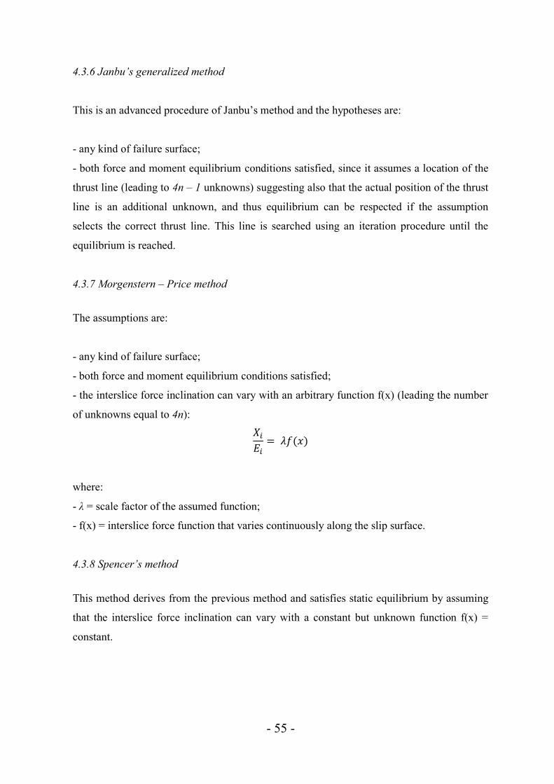
Fig. 4.7 – Presentation of the most common mos methods (Fredlund and Krahn 1977)

The above diagram permits to understand the differences between the FOS from the various

methods, and to study the influence of the selected interslice force function.

Two of the assumptions of the Bishop’s simplified method (BSM) are the not consideration

of the interslice vertical shear forces and the solution only for the moment equilibrium. For

the GLE terminology if the shear forces Xi = 0 means that λ = 0, and the FOS for the BSM

falls in the moment curve in Figure 4.7 where lambda is zero.

A similar consideration can be done for the Janbu’s simplified method (JSM) that also

ignores the interslice vertical forces Xi satisfying only the force equilibrium: the FOS for the

JSM falls in the vertical axis of the diagram where λ = 0 on the force curve.

The Morgenstern and Price method (M-PM) and the Spencer method (SM) satisfy both

moment and force equilibrium: for this reasons their FOS falls where the two curves cross,

and the distinction on which of these methods fall on the crossover point depends on the

chosen interslice force function (constant X/E ratio for SM and any general appropriate

function for M-PM).

Other methods like the Corps of Engineers and the Lowe-Karafiath have the FOS falling on

the force curve, since they only respect the force equilibrium.

- 59 -

4.3.13 Considerations on the interslice force function

The interslice shear force Xi is assumed to be associated to the interslice normal force Ei by

the equation Xi/Ei = λf(x). f(x) can’t be determine for a general problem and the different

methods apply different values for the function.

A case where f(x) = 1.0 is equivalent to the Spencer method (where f(x) is considered a

constant value) and can be used for sandy soils. In fact, sandy soils means an effective

cohesion c’ = 0; the MC expression can be applied to the interslice force relation (Xi/Ei =

tanϕ’) and so the value of λ results equal to tanϕ.

f(x) = senx is an alternative very used as the association of the f(x) to a trapezoidal or

clipped-sine shape (Fig. 4.8, [3]): these types of function are very used for methods like

Morgenstern-Price and GLE where both moment and force equilibriums are satisfied

simultaneously.

Fig. 4.8 – Shape of interslice force functions

In general, the most commonly used functions are the constant and the half-sine functions.

The half sine function is used by default by SLOPE/W program also because this particular

function tends to concentrate the interslice shear forces towards the middle of the sliding

mass and diminishes the interslice shear in the crest and toe areas (SLOPE/W tutorial

manual).

Sarma’s method uses an equation similar to the MC expression to relate the interslice shear

and normal forces (X = ch + Etanϕ): this approach can result interesting due to the

correlation between the material properties and the interslice forces, but actually can be

- 60 -

useful only in cases of cohesion equal to zero (as specified before), where the interslice

shear becomes directly proportional to the normal force. If a cohesion value is specified, the

interslice shear force X starts to become independently of the interslice normal force E,

leading to convergence difficulties (SLOPE/W tutorial manual).

4.3.14 Summary of the method of slices approaches

The methods discussed in the previous paragraphs present some similarities and some

differences. Table 4.2 reassumes these concepts.

Table 4.2. Summary of LE method of slices.

Method ∑F = 0 ∑M = 0 Assumptions

Fellenius/OMS - √ Neglects both Xi and Ei

Bishop’s rigorous √ √ Xi = λ f(x)

Bishop’s simplified √* √ Xi = 0

Janbu’s simplified √ - Xi = 0

Janbu’s generalized √ √** Considers Xi and Ei acting on the thrust line

Morgenstern and Price √ √

Spencer √ √ Constant inclination (Xi/Ei = const)

Lowe – Karafiath √ - Resultant inclination at

Corps of Engineers √ - Two hypotheses on Sarma √ √ For general blocks,

*= force equilibrium only for Ei

** = M equilibrium satisfied if thrust line position correctly selected

Fellenius method is the easier method and its factor of safety can be easily obtained without

any iterative calculation and can be solved by hand or spreadsheet calculation; it’s well

known to be very conservative since sometimes it presents results that can be 20-30 %

higher than those obtained with other methods. For this reason it’s now rarely used in

practice.

- 61 -

The Bishop’s method is one of the most worldwide used methods even if its use has been

reccomanded only for circular failure surfaces (Abramson et al., 2002), but its analysis is

simple for hand calculation and the convergence is fast.

Janbu’s simplified method presents only few convergence problems and can be used also for

a non circular failure surfaces which is commonly observed in sandy-type soils.

The Janbu’s rigorous method consists in the introduction of the correction factor f0 but the

methods to calculate this factor are based on limited case studies and for this reason the use

of these factors are questioned for some engineers if applied to complicated non-

homogeneous soil slopes.

Morgernstern-Price and Spencer methods consider both force and moment equilibriums and

being careful to the thrust line position are two methods suggested by computer softwares

like SLOPE/W, since they meet the criteria of fulfillment of all equations of statics

considering both shear and normal interslice forces.

The Lowe-Karafiath method and the Corps of Engineers methods are based on hypotheses

on the interslice force functions and satisfy only the moment equilibrium; usually the first

one gives results close to that obtained with the Janbu’s rigorous method even though the

moment equilibrium is not satisfied. The Corps of Engineers method in some cases may lead

to a high factor of safety, and to account this problem some engineers prefer to adopt a

lower inter-slice force angle (Duncan and Wright, 2005).

Sarma’s method is particular due to the hyphoteses made on the interslice force function

equation, as explained in the previuos paragraph, but in some cases (soils with zero

cohesion) it can be very useful.

The General limit equilibrium formulation is usually adopted to provide a framework for

discussing, describing and understanding all the other methods, since it can compare the

various FOS of the other methods (SLOPE/W tutorial manual). The main difficulty in using

the GLE procedure is related to the requirement that the user verify the reliability and

reasonableness of the calculated safety factor, preventing its use for automatic search

techniques that try to identify the critical failure surface (Favaretti, 2010).

Regarding the factor of safety values, Ambramson et al. (2002) found that for circular

failure surfaces the Bishop’s simplified method always gives higher FOS values than

Janbu’s simplified method; this value falls within ± 5% of the safety factor calculated with

the more rigorous methods. However, the safety factor can differ by ± 15% as compared

with the results calculated by Spencer and Morgenstern-Price methods.

- 62 -

4.4 General concepts of Finite Element Method

Limit element methods are based on the assumptions that results give stresses and forces

that satisfy force equilibrium of each slice making also the same safety factor for each of

them. These concepts lead to some limitations related to the impossibility to obtain realistic

stress distributions along the slip plane or within the potential sliding mass. In order to

consider also this question, the finite element approach establishes the stress distribution in

the ground surface and then applies these stresses in a stability analysis.

Finite Element Method (FEM) is a numerical analysis based on differential equations to

solve problems of engineering and mathematical physics useful for cases with complicated

geometries, loadings and material properties. This method was originated from the need to

solve complex elasticity and structural analysis problems in civil and aeronautical

engineering and then developed also to other branches of the engineering.

FEM is based on a simplified physical model that wants to represent the real object

characteristics under investigation by using mathematical models based on a discretization

procedure.

The discretization consists in dividing the model body into an equivalent system of many

smaller bodies or units (finite elements) interconnected at points common to two or more

elements (nodes) and or boundary lines and/or surfaces.

Reassuming, the key factors of the geometry of a FEM (Fig. 4.9) are:

- points: determine the start and end of lines and can be used also to define concentrated

loads;

- lines: are used to define physical boundaries of the geometry, the model boundaries and

discontinuities in the geometry (for example walls or separation of distinct soil layers);

- clusters: are areas that are fully enclosed by lines and defines zones where the soil

properties are homogeneous.

When the geometry model is complete a finite element model can be formed, basing on the

composition of clusters and lines of the geometry model.

- 63 -

Fig. 4.9 – Components of the geometry model of a FE analysis

The three key components of a finite element mesh are (Fig. 4.10):

- finite elements: smaller (usually triangular) units in which cluster is divided;

- nodes: points that define the elements and usually there are 15-node elements or 6-node

elements. Adjacent elements are connected through their common nodes. The displacement

are calculated at the nodes during the FE analysis.

- stress points: points where stress and strain are calculated. A 15-node triangular element

contains 12 stress points and 6-node triangular elements has 3 stress points.

Fig. 4.10 – Components of a finite element mesh

In this thesis the study with the FEM of the slope stability of Este’s landfill is done using the

PLAXIS program, a finite element software that has been developed specifically for the

analysis of deformation and stability in geotechnical engineering projects.

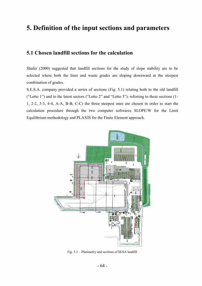
- 64 -

5. Definition of the input sections and parameters

5.1 Chosen landfill sections for the calculation

Shafer (2000) suggested that landfill sections for the study of slope stability are to be

selected where both the liner and waste grades are sloping downward at the steepest

combination of grades.

S.E.S.A. company provided a series of sections (Fig. 5.1) relating both to the old landfill

(“Lotto 1”) and to the latest sectors (“Lotto 2” and “Lotto 3”): referring to these sections (1-

1, 2-2, 3-3, 4-4, A-A, B-B, C-C) the three steepest ones are chosen in order to start the

calculation procedure through the two computer softwares SLOPE/W for the Limit

Equilibrium methodology and PLAXIS for the Finite Element approach.

Fig. 5.1 – Planimetry and sections of SESA landfill

- 65 -

The cross sections studied are:

- 4-4: it’s located in the south – western part of the site and refers only to the oldest landfill

named “Lotto 1”; its study is important to evaluate the stability of the oldest part of S.E.S.A.

landfill. Another reason is because in the northwest part of “Lotto 1” a new dumping area

has been designed (“Lotto Ovest”) leading the evaluation of the stability of the near old site

as an issue of particular importance. Moreover, older waste presents a higher organic

fraction content than those dumped after an appropriate separate collection system (that

started with the fill of “Lotto 2”): this condition can lead to a higher instability if compared

to the other situations due to the higher water content into the waste mass. In addition, old

landfill presents a final top cover very different if related to the other protection types of the

landfill without any type of bottom liner systems. The analysis (as also for the other chosen

sections) has been performed considering only an half of the section (Fig. 5.2); indeed the

two halves are almost equals both in shape as also for the top and bottom liner systems. This

section has the highest point at about 15 meters from the ground surface and presents a long

part of the section (about 36 m) practically linear and two steepest slopes (the first of 12 m

of horizontal length, the second of 6 m) of 31 degrees, divided by a berm of 8 meters. The

landfill bottom (about 3 m below the ground surface) doesn’t present any type of protection

but is placed inside a natural clay barrier with some silty layers.

Fig. 5.2 – Left half part of section 4-4

- 66 -

- 2-2: it presents a steepest inclination if compared to section 1-1 and is near to other

S.E.S.A. waste treatment activities like the composting and anaerobic digestion plant. This

part is composed by “Lotto 1” and “Lotto 3” dumping zones; the study of the slope stability

of this section is important because in the northern part of “Lotto 3” there are other S.E.S.A.

waste treatment activities (such as the composting treatment plant, Fig. 2.8) and the

verification that the landfill slope is stable is fundamental primarily to guarantee the safety

of the onsite workers and to not cause any damage to other neighboring activities.

The analysis is performed considering the left half section (Fig. 5.3), even if the two half

sections are not completely equal. The right section presents the union between the old

landfill and “Lotto 3”, and, as previously said, the bottom barrier system of the old landfill

part doesn’t present any type of protection; anyway, the stability of “Lotto 1” has been

already analyzed with section 4-4. This section has the maximum height at about 20 m from

the ground surface and presents a long (124 m) and almost flat surface followed by a 31

degrees slope with a horizontal length of 13 m, a berm and another 31 degrees slope

(horizontal length = 7 m). The slope has natural soil/compost and clay as protection.

Fig. 5.3 - Left half part of section 2-2

- A-A: it has a steepest inclination if compared to section B-B. Its study is done without

considering the future landfill extension (“Lotto Ovest” in this case) because no waste has

been dumped in this new area (delimitated by the red line) that it’s only been designed for

future landfilling operations. Section A-A (Fig. 5.4) is formed by “Lotto 2” and “Lotto 3”

dumping zones and, as described in the landfill description chapter, on the left side there will

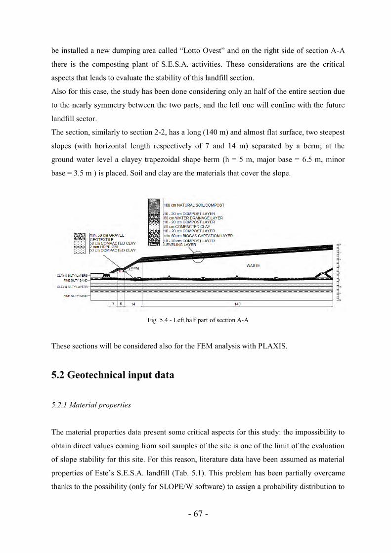
- 67 -

be installed a new dumping area called “Lotto Ovest” and on the right side of section A-A

there is the composting plant of S.E.S.A. activities. These considerations are the critical

aspects that leads to evaluate the stability of this landfill section.

Also for this case, the study has been done considering only an half of the entire section due

to the nearly symmetry between the two parts, and the left one will confine with the future

landfill sector.

The section, similarly to section 2-2, has a long (140 m) and almost flat surface, two steepest

slopes (with horizontal length respectively of 7 and 14 m) separated by a berm; at the

ground water level a clayey trapezoidal shape berm (h = 5 m, major base = 6.5 m, minor

base = 3.5 m ) is placed. Soil and clay are the materials that cover the slope.

Fig. 5.4 - Left half part of section A-A

These sections will be considered also for the FEM analysis with PLAXIS.

5.2 Geotechnical input data

5.2.1 Material properties

The material properties data present some critical aspects for this study: the impossibility to

obtain direct values coming from soil samples of the site is one of the limit of the evaluation

of slope stability for this site. For this reason, literature data have been assumed as material

properties of Este’s S.E.S.A. landfill (Tab. 5.1). This problem has been partially overcame

thanks to the possibility (only for SLOPE/W software) to assign a probability distribution to

- 68 -

all input parameters. In this way, a variability of the input parameters is considered.

Moreover, most of the materials are naturally formed materials and their physical properties

vary from point to point even if parts of an apparently homogeneous soil. Laboratory results

found that most soil properties can be considered as random variables corresponding to a

normal distribution function (SLOPE/W tutorial manual). For these reasons, the input

parameters for SLOPE/W software (i.e. cohesion, friction angle and unit weight) are been

assumed to be normally distributed.

In addition, once that the calculation procedure is completed, a Monte Carlo scheme (with

2000 Monte Carlo trials) is used to compute a probability distribution of the resulting safety

factors.

Data regarding the subsoil are taken from data regarding investigations on soils with similar

characteristics located in the proximity of the site of interests and typical literature values.

The values of cohesion and angle of internal friction are been diminished by some

corrective-precautionary factors (1.25 both for c and tanϕ) as required by the Italian

normative NTC 08. The corrective factor relating to the unit weight is 1.0.

Table 5.1. Material properties for Este’s S.E.S.A. landfill (MC model).

MATERIAL Dry unit weight

(kN/m3)

Saturated unit weight

(kN/m3)

Cohesion (kPa)

Internal friction angle (°)

Young’s modulus (kN/m2)

Poisson’s ratio

(-) Reference

Natural soil 11.0 16.0 8.0 19.6 2000 0.2 Pistolato (2013)

Compost 6.8 16.4 0 14.8 5000 0.25 Omari et al. (2012) Compacted

clay 16.0 18.0 24.0 29.2 20000 0.4 Look (2007)

Leveling layer 18.2 21.2 0 33.8 100000 0.35 Omari et al. (2012)

Gravel 18.0 20.0 0 28.3 75000 0.3 Look (2007) Clay with silty

layers 17.0 18.0 4.0 20.4 12000 0.4 Soil investigations and literature data

Fine silty sand 16.0 19.0 0 24.7 15000 0.3 Soil investigations and literature data

Clay with silty layers and peat 16.0 18.0 4.0 20.4 12000 0.35 Soil investigations

and literature data Gray fine silty

sand 16.0 20.0 0 33.8 20000 0.3 Soil investigations and literature data

5.2.2 Waste properties considerations

The issue relating to the waste properties is very delicate. In fact, MSW have some

constitutive similarities in common with natural soils, but they present also particular

characteristics as the great deformability for some elements present in the MSW, a physical

- 69 -

and mechanical instability of the organic components and the presence of pore fluids, i.e.

leachate and biogas (Favaretti, 2010).

Although waste is heterogeneous, many studies show that municipal solid waste has

mechanical properties that vary in a consistent and predictable way (Dixon et al., 2004).

Shear strength parameters

Regarding the shear strength parameters, the factors that affect their behavior are:

compressibility, organic and fiber content of waste and degradation extent (Dixon et al.,

2004). Tests carried out at the University of Rome (1995) were part of a research program

aimed at the mechanical characterization of waste based on in situ and laboratory tests and

on the systematic observation of the behavior of Italian landfills (Grisolia et al., 1995).

Triaxial tests were conducted on artificially reconstructed waste samples in order to simulate

the waste characteristics. The composition of the waste studied was: cloth and wood 6%,

paper 32%, plastic 8%, rubble 32% and organic matter 22%, with a water content w = 40%.

Preliminary tests, like some compressibility measurements, were carried out in order to

verify that the behavior and characteristics of the reconstructed material matches the

undisturbed waste samples taken from the landfill.

The results indicated that adopting a level of deformations similar to that commonly found

for soils at the scale of laboratory samples (named 15-20%), the shear strength values that

could be adopted for waste landfill are a cohesion values c = 5 - 10 kPa and a friction angle

of about ϕ = 24°- 30°. Other studies (Dixon et al., 2004) conducted with direct shear tests,

shown a cohesion between 0 and 24 kPa and an angle of internal friction varying between 22

and 42 degrees. For design situations, a cohesion value in the range of 0-30 kPa and an

internal friction angle of 20-35° would seem reasonable values (Omari, Boddula, 2010).

Unit weight

Factors that govern the unit weight are principally waste composition and landfill

operational practices (compaction effort, cover soil placement and liquid management)

during waste placement and the effective confining stress currently acting on the waste;

although the scarcity of literature data about MSW unit weights, internally consistent waste

composition and waste handling practices and predictable confining stress effects suggest

- 70 -

the existence of a characteristic profile of unit weight versus depth for many landfills. Based

upon analysis of available laboratory and field data, a characteristic MSW unit weight

profile represented by a hyperbolic function was found to exist for individual landfills

(Zekkos et al., 2006). Figure 5.5 shows this trend for tests carried out for some landfills.

Another study (Fassett et al., 1994) indicated some statistical values for MSW unit weight

considering different literature data: for good compaction conditions, a value of around 10.0

kN/m3 is normally accepted for design conditions.

Fig. 5.5 – MSW unit weight trends from in situ tests for individual landfills (Zekkos et al., 2006)

Compressibility

Mechanisms related to waste compression have been summarized by Manassero et al.

(1996) as listed in Table 5.2.

Table 5.2. Mechanisms of waste compression and factors controlling magnitude of

settlement (Manassero et al., 1996).

- 71 -

It can be assumed that the total settlement is composed by two main components: a primary

and a secondary compression. Primary compression consists in the physical compression of

particles (distortion, bending, crushing and particle orientation) and consolidation

(especially for saturated waste bodies). Usually, this type of compression occurs in a short

period of time (few days or few weeks) and incrementally linear compression models can be

used to calculate primary settlements. Secondary compression includes creep effects

(mechanical compression under constant stress) and degradation processes (chemical and

biological); biodegradation is the main component for the secondary compression, and can

be influenced by a wide range of interrelated factors (moisture content, temperature and

stress level) varying spatially and timing within the landfill.

Lateral stiffness

Stiffness parameters like shear modulus G, Young’s modulus E and Poisson’s ratio υ are

used to quantify the response of a material to a change in stress. These parameters are

related by the equation:

Tests conducted by Dixon and Jones (1998) and Dixon et al. (2000) on MSW samples

observed a general trend of increasing stiffness with stress (and hence also with depth) level,

with the older waste (12-15 years old and partly degraded) that appears to be less stiff than

fresh waste (1-5 years old).

Horizontal in situ stress

The difficulty to measure in situ vertical stress of MSW is related to the act of introducing a

measuring instrument that alter the stress being measured (Dixon et al., 2004). For a body at

rest, horizontal stress σh can be related to vertical stresses σv by the coefficient of each

pressure at rest K0:

- 72 -

A laboratory study made by Landva et al. (2000) concluded that K0 for fresh waste would be

equal to about 0.35-0.4, while for MSW with less reinforcing material than the sample

analyzed would have a K0 value around to 0.5.

Hydraulic properties

Hydraulic conductivity of waste is important due to the influence on the leachate pressure

distribution and hence on the magnitude and distribution of effective stresses and therefore

on shear strength. The heterogeneity nature of MSW varying point to point the waste

permeability but field and laboratory studies provided some important considerations.

Waste structure, the use of low permeability daily cover layers and stress levels play the

major role to determine hydraulic waste conductivity (Dixon et al., 2004). A study

conducted by Powrie and Beaven (1999) found that the permeability of non-degraded MSW

could diminish by over three orders of magnitude to approximately 10-8 m/s between

placement and burial to a depth of 60 m due to compression.

5.2.3 Waste properties for Este’s landfill

MSW properties for Este’s landfill are been selected considering the different landfill

sectors analyzed. “Lotto 1” (studied with section 4-4) is the old landfill of Este that was

active since the 60s until the 1995 when a separate collection system was completely absent.

Due to the impossibility to establish waste values directly for this old site, literature data

([15], [28]) are been implemented, considering top and bottom waste data obtained from old

MSW landfills (Tab. 5.3).

Table 5.3. Waste properties for “Lotto 1”.

MATERIAL Dry unit weight

(kN/m3)


(kN/m3)

Cohesion (kPa)



Poisson’s ratio

(-) Top waste (5 m) 9.4 10.8 10.0 30.0 1000 0.25

Bottom waste 11.0 15.4 30.0 20.0 2500 0.45

These values seems reasonable: older and deeper waste present a high cohesion and a low

friction angle due to the increased fineness of the waste thanks to degradation processes,

while for more recently dumped waste a low cohesion and a high friction angle can be

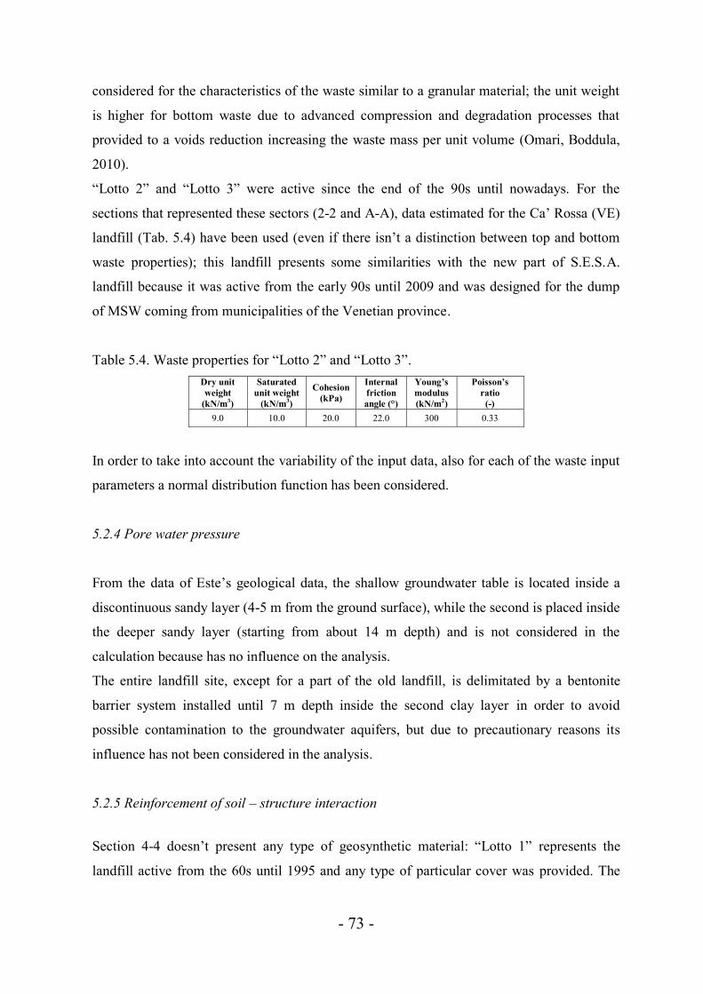
- 73 -

considered for the characteristics of the waste similar to a granular material; the unit weight

is higher for bottom waste due to advanced compression and degradation processes that

provided to a voids reduction increasing the waste mass per unit volume (Omari, Boddula,

2010).

“Lotto 2” and “Lotto 3” were active since the end of the 90s until nowadays. For the

sections that represented these sectors (2-2 and A-A), data estimated for the Ca’ Rossa (VE)

landfill (Tab. 5.4) have been used (even if there isn’t a distinction between top and bottom

waste properties); this landfill presents some similarities with the new part of S.E.S.A.

landfill because it was active from the early 90s until 2009 and was designed for the dump

of MSW coming from municipalities of the Venetian province.

Table 5.4. Waste properties for “Lotto 2” and “Lotto 3”. Dry unit weight

(kN/m3)


(kN/m3)

Cohesion (kPa)



Poisson’s ratio

(-) 9.0 10.0 20.0 22.0 300 0.33

In order to take into account the variability of the input data, also for each of the waste input

parameters a normal distribution function has been considered.

5.2.4 Pore water pressure

From the data of Este’s geological data, the shallow groundwater table is located inside a

discontinuous sandy layer (4-5 m from the ground surface), while the second is placed inside

the deeper sandy layer (starting from about 14 m depth) and is not considered in the

calculation because has no influence on the analysis.

The entire landfill site, except for a part of the old landfill, is delimitated by a bentonite

barrier system installed until 7 m depth inside the second clay layer in order to avoid

possible contamination to the groundwater aquifers, but due to precautionary reasons its

influence has not been considered in the analysis.

5.2.5 Reinforcement of soil – structure interaction

Section 4-4 doesn’t present any type of geosynthetic material: “Lotto 1” represents the

landfill active from the 60s until 1995 and any type of particular cover was provided. The

- 74 -

other two sections presents a geotextile and a 2 mm HDPE geomembrane as parts of the

bottom barrier system.

In order to consider the geosynthetics contribution, the SLOPE/W program considers some

reinforcement parameters. The first is the factored pullout resistance (FPR) per unit length

of geosynthetic (kN/m/m) that is intended as the applied bond resistance of the fabric to the

soil. Considering a factor of safety (FS) dependency, this factor is calculated as:

where:

- PR = calculated pullout resistance (kPa), the skin friction of the reinforcement bond;

- SIA = interface adhesion (kPa), the cohesion at the contact point between material and

geosynthetic;

- σ’v = the effective overburden stress (kPa), directly calculated by the program according to

the position of the geosynthetic;

- δ = interface shear angle (°), the contact angle between material and geosynthetic;

- SAF = surface area factor (interface factor, between 0 and 2), used at the contact point

between the fabric and the soil;

- RRF = resistance reduction factor (-) to account for nonlinear distribution stress reduction

over the embedded length.

The second reinforcement parameter is the factored tensile capacity (FTC), i.e. the

maximum pullout force that has not to be exceed. It’s defined as:

where:

- TC = tensile capacity (kN), the maximum capacity that the reinforcement can bear without

breaking;

- RF = reduction factor (-) to take into account installation damage, creep and durability.

Parameters considered for 2 mm HDPE geomembrane:

SIA = 0 kPa (cautionary value), δ = 25°, SAF = 1, RRF = 1.5, TC = 249 N, RF = 1.

- 75 -

Parameters considered for the non woven PP geotextile:

SIA = 0 kPa, δ = 30°, SAF = 1, RRF = 1.5, TC = 725 N, RF = 1.

5.2.6 Imposed loading

The loading imposed to the system is the seismic contribution, inputting the two seismic

coefficients previously found (Paragraph 3.4): KH = 0.002 and KV = 0.001.

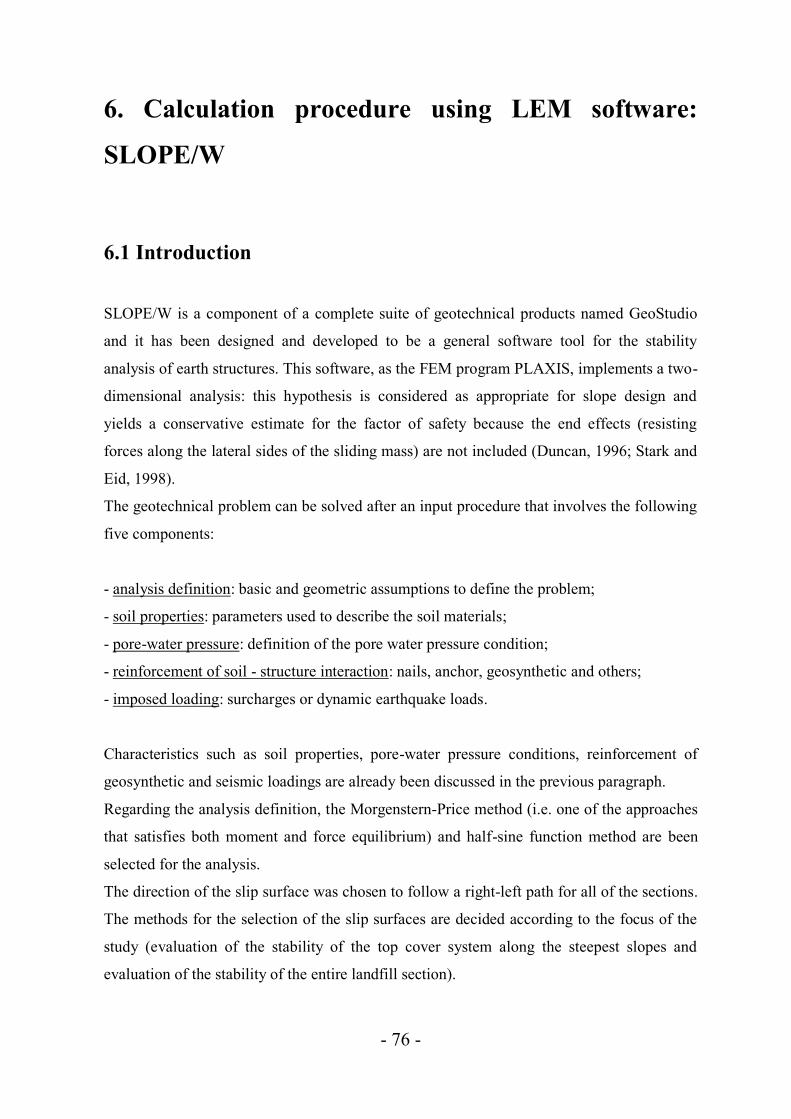
- 76 -

6. Calculation procedure using LEM software:

SLOPE/W

6.1 Introduction

SLOPE/W is a component of a complete suite of geotechnical products named GeoStudio

and it has been designed and developed to be a general software tool for the stability

analysis of earth structures. This software, as the FEM program PLAXIS, implements a two-

dimensional analysis: this hypothesis is considered as appropriate for slope design and

yields a conservative estimate for the factor of safety because the end effects (resisting

forces along the lateral sides of the sliding mass) are not included (Duncan, 1996; Stark and

Eid, 1998).

The geotechnical problem can be solved after an input procedure that involves the following

five components:

- analysis definition: basic and geometric assumptions to define the problem;

- soil properties: parameters used to describe the soil materials;

- pore-water pressure: definition of the pore water pressure condition;

- reinforcement of soil - structure interaction: nails, anchor, geosynthetic and others;

- imposed loading: surcharges or dynamic earthquake loads.

Characteristics such as soil properties, pore-water pressure conditions, reinforcement of

geosynthetic and seismic loadings are already been discussed in the previous paragraph.

Regarding the analysis definition, the Morgenstern-Price method (i.e. one of the approaches

that satisfies both moment and force equilibrium) and half-sine function method are been

selected for the analysis.

The direction of the slip surface was chosen to follow a right-left path for all of the sections.

The methods for the selection of the slip surfaces are decided according to the focus of the

study (evaluation of the stability of the top cover system along the steepest slopes and

evaluation of the stability of the entire landfill section).

- 77 -

The slip surface has been considered to have 30 slices, each with a minimum depth of 0.1 m

and a minimum slice width of 0.1 m.

One of the basic assumptions which has to be made to solve the problem (i.e. to find the

minimum factor of safety for the critical failure surface) is the definition of the method to

find the failure surfaces.

6.2 Slip surface shapes

One of the key argument in a slope stability analysis is the determination of the position of

the critical slip surface with the lowest factor of safety. This procedure is done with a trial

operation, creating possible slip surfaces and computing the associated FOS. Once that the

procedure is complete, the trial slip surface with the lowest safety factor is considered as the

critical slip surface.

There are many different methods to define the shape and positions of trial slip surfaces; in

this chapter the two most used methods are presented, considering examples provided by

SLOPE/W tutorial manual.

6.2.1 Grid and radius method

The trial slip surface is an arc of circle that is a portion of a circle that cuts through the

slope; the circle can be defined specifying the centre and the radius. Many slip surfaces can

be specified defining a grid of circle centers and a range of defined radii.

An example taken from the SLOPE/W tutorial manual is shown is Fig. 6.1.

Fig. 6.1 – Grid and radius method

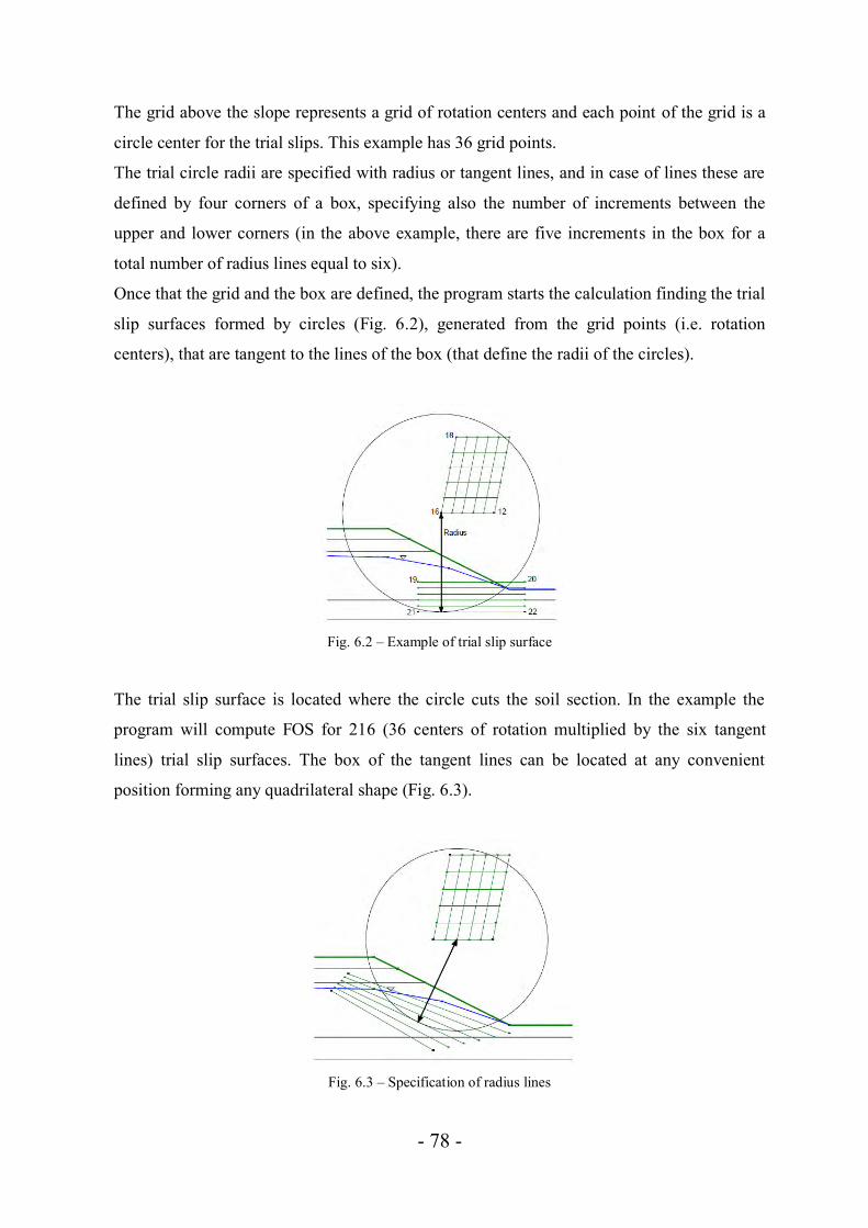
- 78 -

The grid above the slope represents a grid of rotation centers and each point of the grid is a

circle center for the trial slips. This example has 36 grid points.

The trial circle radii are specified with radius or tangent lines, and in case of lines these are

defined by four corners of a box, specifying also the number of increments between the

upper and lower corners (in the above example, there are five increments in the box for a

total number of radius lines equal to six).

Once that the grid and the box are defined, the program starts the calculation finding the trial

slip surfaces formed by circles (Fig. 6.2), generated from the grid points (i.e. rotation

centers), that are tangent to the lines of the box (that define the radii of the circles).

Fig. 6.2 – Example of trial slip surface

The trial slip surface is located where the circle cuts the soil section. In the example the

program will compute FOS for 216 (36 centers of rotation multiplied by the six tangent

lines) trial slip surfaces. The box of the tangent lines can be located at any convenient

position forming any quadrilateral shape (Fig. 6.3).

Fig. 6.3 – Specification of radius lines

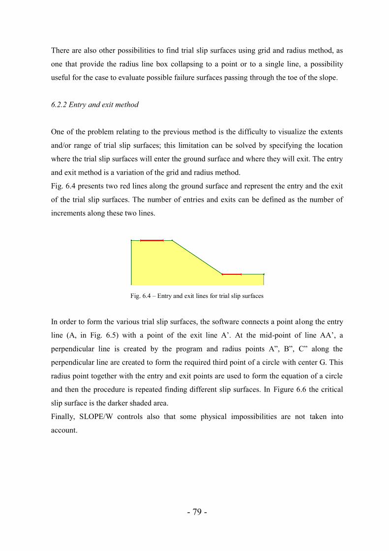
- 79 -

There are also other possibilities to find trial slip surfaces using grid and radius method, as

one that provide the radius line box collapsing to a point or to a single line, a possibility

useful for the case to evaluate possible failure surfaces passing through the toe of the slope.

6.2.2 Entry and exit method

One of the problem relating to the previous method is the difficulty to visualize the extents

and/or range of trial slip surfaces; this limitation can be solved by specifying the location

where the trial slip surfaces will enter the ground surface and where they will exit. The entry

and exit method is a variation of the grid and radius method.

Fig. 6.4 presents two red lines along the ground surface and represent the entry and the exit

of the trial slip surfaces. The number of entries and exits can be defined as the number of

increments along these two lines.

Fig. 6.4 – Entry and exit lines for trial slip surfaces

In order to form the various trial slip surfaces, the software connects a point along the entry

line (A, in Fig. 6.5) with a point of the exit line A’. At the mid-point of line AA’, a

perpendicular line is created by the program and radius points A”, B”, C” along the

perpendicular line are created to form the required third point of a circle with center G. This

radius point together with the entry and exit points are used to form the equation of a circle

and then the procedure is repeated finding different slip surfaces. In Figure 6.6 the critical

slip surface is the darker shaded area.

Finally, SLOPE/W controls also that some physical impossibilities are not taken into

account.

- 80 -

Fig. 6.5 – Scheme of the entry and exit method

Fig. 6.6 – Critical slip surfaces

6.3 Analysis of section 4-4

The section can be directly imported from the AUTOCAD program to the SLOPE/W

software and the different steps for the analysis can be initialized (Fig. 6.7).

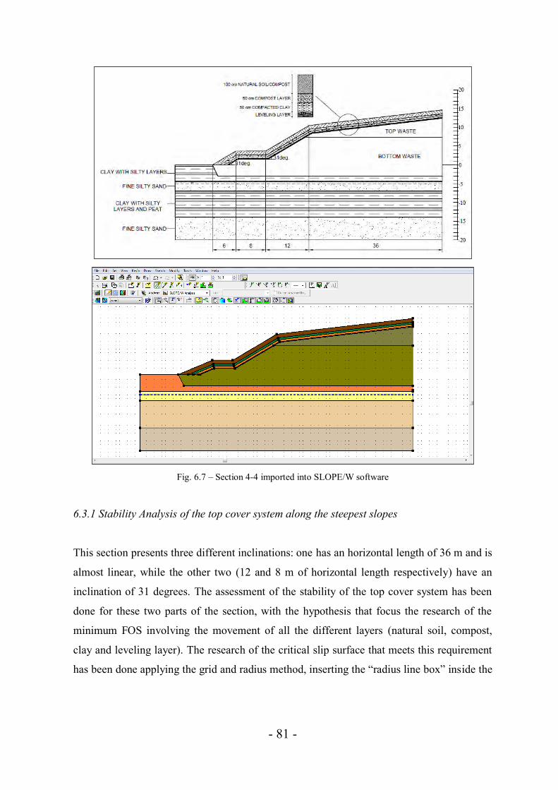
- 81 -

Fig. 6.7 – Section 4-4 imported into SLOPE/W software

6.3.1 Stability Analysis of the top cover system along the steepest slopes

This section presents three different inclinations: one has an horizontal length of 36 m and is

almost linear, while the other two (12 and 8 m of horizontal length respectively) have an

inclination of 31 degrees. The assessment of the stability of the top cover system has been

done for these two parts of the section, with the hypothesis that focus the research of the

minimum FOS involving the movement of all the different layers (natural soil, compost,

clay and leveling layer). The research of the critical slip surface that meets this requirement

has been done applying the grid and radius method, inserting the “radius line box” inside the

- 82 -

top cover system (Fig. 6.8): the grid has 36 centers of rotation with six tangent lines, with

the possibility to obtain 216 factors of safety.

Fig. 6.8 – Application of the grid and radius method to find the critical slip surface for the first slope of section

4-4

The minimum calculated factor of safety, that is the only one of the entire study minor than

1.0 (FOS = 0.99) involves a movement only for soil and compost layers (Fig. 6.9a), while a

higher safety factor (FOS = 2.00) regards the instability of the first slope considering the

entire top barrier system (Fig. 6.9b).

Fig. 6.9 a,b – Critical slip surfaces that involves the top barrier system for the first slope of section 4-4

The analysis on the second steepest slope of the 4-4 section (the nearest one to the ground

surface) has been done with the same hypothesis of the previous slope, implementing a grid

and radius method for searching the critical failure surface and inserting the radius box

inside the cover system (Fig. 6.10). Similarly to the previous slope, the minimum critical

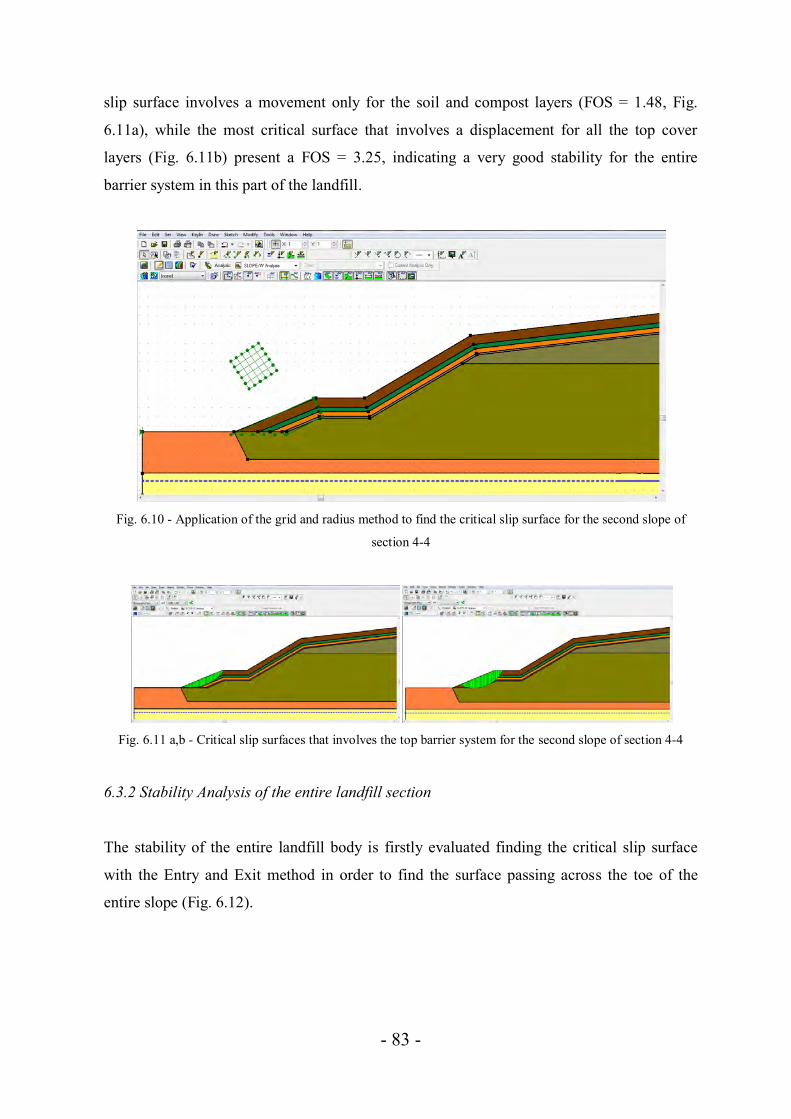
- 83 -

slip surface involves a movement only for the soil and compost layers (FOS = 1.48, Fig.

6.11a), while the most critical surface that involves a displacement for all the top cover

layers (Fig. 6.11b) present a FOS = 3.25, indicating a very good stability for the entire

barrier system in this part of the landfill.

Fig. 6.10 - Application of the grid and radius method to find the critical slip surface for the second slope of

section 4-4

Fig. 6.11 a,b - Critical slip surfaces that involves the top barrier system for the second slope of section 4-4

6.3.2 Stability Analysis of the entire landfill section

The stability of the entire landfill body is firstly evaluated finding the critical slip surface

with the Entry and Exit method in order to find the surface passing across the toe of the

entire slope (Fig. 6.12).

- 84 -

Fig. 6.12 – Slope stability analysis of the entire section 4-4 (failure surface passing through the toe)

The slope results to be very stable: FOS = 2.02, showing a critical failure surface passing

through the toe of the slope passing also through the landfill bottom (that doesn’t present

any type of barrier for this old landfill part).

It has been evaluated also the stability where the critical slip surface could pass through the

ground surface (Fig. 6.13); this part of soil will be interested by the future designed landfill

enlargement (“Lotto Ovest”, Fig. 5.1). The FOS = 1.88 indicates a good stability also for

this case.

Fig. 6.13 - Slope stability analysis of the entire section 4-4 (failure surface passing through the base)

- 85 -

Another possible critical failure surface could be the one passing through the bottom of the

landfill body; this possible failure case has been considered with the application of the grid

and radius method, applying the radius box inside the location of the landfill bottom (about

3 m depth. The calculation (Fig. 6.14) gives results indicating a very high stability also for

this case: FOS = 2.24 for Morgenstern-Price method.

Fig. 6.14 – Slope stability analysis of the entire section 4-4 (failure surface passing through landfill bottom)

6.3.3 Stability Analysis of the entire landfill section varying waste parameters

All the calculated FOS for the stability of the entire landfill body present very safety

conditions, but as previously discussed the waste parameters are very variables and obtained

from literature data; for these reasons, a study has been conducted in order to establish how

the FOS can vary using different waste characteristics to find which might be the worst

situations.

It has been calculated the safety factor using Morgenstern-Price method, analyzing nine

possible combinations for different waste input parameters: as suggested by some studies

([9], [42]) a value of about 10.0 kN/m3 as unit weight can be normally accepted for all of the

waste strata, and as suggested by a study conducted on MSW Italian landfills (Grisolia et al.,

1995), shear strength parameters are been varied between 0 and 10 kPa for the cohesion and

20 and 30 degrees for the internal friction angle (these trial and precautionary parameters are

considered as already reduced by the corrective factor of NTC). The study has been

conducted for failure surfaces passing both at the toe of slope and on the base of ground

- 86 -

surface, and for slip surfaces passing through the landfill bottom, always considering a

Monte Carlo scheme with 2000 trials and a normal probability density functions for the

input parameters. Results are listed in Tables 6.1.

Table 6.1. Stability analysis for section 4-4 varying waste characteristics.

Unit

weight (kN/m3)

Cohesion (kPa)


FOS for circular failure surface passing…

at the slope toe

through the base

through the landfill bottom

Type 1 10 0 20 1.14 1.16 1.71 Type 2 10 0 25 1.43 1.45 2.14 Type 3 10 0 30 1.76 1.77 2.51 Type 4 10 5 20 1.49 1.49 1.97 Type 5 10 5 25 1.79 1.79 2.35 Type 6 10 5 30 2.11 2.10 2.72 Type 7 10 10 20 1.80 1.79 2.22 Type 8 10 10 25 2.11 2.05 2.56 Type 9 10 10 30 2.45 2.24 2.93

The worst cases are, as expected, those related to the lower shear strength values; however,

the stability is respected also in these cases. In Chapter 8 a sensitivity analysis on the

parameters and considerations on the calculated factors of safety are presented.


As for section 4-4, the section is directly imported from the AUTOCAD program to the

SLOPE/W software and the different steps for the analysis can be initialized (Fig. 6.15).

- 87 -

Fig. 6.15 – Section 2-2 imported into SLOPE/W software


As section 4-4, also this section presents three different inclinations: one very long (124 m)

and practically linear, while the other two have an inclination of 31 degrees. The assessment

of the stability of the top cover system has been done for these two parts of the section,

assuming that the focus of the study is the research of the minimum FOS involving the

movement of all the different layers (natural soil, compost, gravel, clay and leveling layers).

The research of the critical slip surface that meets this requirement has been done applying

the grid and radius method, inserting the “radius line box” inside the top cover barrier

system. The minimum calculated safety factor (FOS = 2.64) regards the movement only for

- 88 -

a small part of soil, while the lower FOS regarding the movement of the entire top cover

barrier of the first slope (Fig. 6.16) is equal to 3.29, indicating a very good stability for this

part of top cover.

Fig. 6.16 - Critical slip surface that involves the entire barrier system for the first slope of section 2-2

The second steepest slope of section 2-2 (the nearest one to the ground surface) has been

analyzed considering the same hypothesis of the previous slope, implementing a grid and

radius method for searching the critical failure surface and inserting the radius box inside the

cover system. The most critical slip surface that involves all layers is shown in Fig. 6.17.

Fig. 6.17 - Critical slip surface that involves the entire barrier system for the second slope of section 2-2

- 89 -

The result for the M-P method indicates that the slope is very stable (FOS = 2.83) also for

the slope near the base of the 2-2 section; moreover, this value is also the minimum

calculated safety factor and involves all the top cover layers.


The entire landfill body stability is evaluated finding the critical slip surface with the Entry

and Exit method in order to find the surface passing across the toe of the entire slope (Fig.

6.18). The calculated safety factor is equal to 1.75. As for section 4-4, it has been studied

also the stability for cases where the critical slip surface could pass through the ground

surface (Fig. 6.19). For this case, FOS = 1.81.

Fig. 6.18 – Slope stability analysis of the entire section 2-2 (failure surface passing through the toe)

- 90 -

Fig. 6.19 - Slope stability analysis of the entire section 2-2 (failure surface passing through the base)

The grid and radius method has been applied in order to find the critical slip surface passing

through the landfill bottom barrier, which is formed by a leachate drainage layer (min. 50

cm), geotextile, clay (50 cm), 2 mm HDPE geomembrane and 50 cm of clay (Fig. 6.20). The

safety factor results equal to 3.05 indicating a very good stability, with a circular failure

surface passing through the geosynthetics and bottom layers (leachate captation layer and

clay) without involving the natural fine silty sand layer.

Fig. 6.20 – Slope stability analysis of the entire section 2-2 (failure surface passing through landfill bottom)

For this section has been evaluated also the sliding stability of bottom materials on the two

geosynthetic liners (a geotextile is placed between the drainage layer and the shallow clay

- 91 -

layer, while a 2 mm HDPE geomembrane subdivides the two clay layers). The analysis is

made with the grid and radius method, considering the material just below the geosynthetic

as impenetrable; in this way the impenetrable layer causes the trial slip surface to follow the

liner. The thin region just above the impenetrable material presents properties representative

of the frictional sliding resistance between the cover material and the liner, i.e. the shear

strength along that portion of the sliding surface that follows the material considered as

impenetrable. The critical slip surface tangent (Fig. 6.21) to the geotextile liner presents a

safety factor equal to 2.24, while for sliding surfaces tangent to the geomembrane (Fig. 6.22)

the FOS results equal to 2.74.

Fig. 6.21 – Sliding stability for failure surfaces tangent to the geotextile liner of section 2-2

Fig. 6.22 – Sliding stability for failure surfaces tangent to the geomembrane liner of section 2-2

- 92 -


As for the previous analyzed section, also the stability of section 2-2 has been studied

considering different waste input parameters (Tab. 5.2) due to the high uncertainty of these

waste values.

The study has been done considering the first three analyzed possible failure mechanisms

(Tab. 6.2), while possible effects of the change of waste input parameters on the

geosynthetic liners are discussed in Chapter 8.

Table 6.2. Stability analysis for section 2-2 varying waste characteristics.

Unit

weight (kN/m3)

Cohesion (kPa)



at the slope toe

through the base



6.5 Analysis of section A-A

The section is firstly drawn with AUTOCAD program and then imported into SLOPE/W

software (Fig. 6.23), considering the three subsectors of “Lotto 3”.

- 93 -

Fig. 6.23 – Section A-A imported into SLOPE/W software


The slope profile is similar to the other two sections, presenting a long slope almost linear

and two other slopes more inclined (30 degrees instead of 31 degrees of the other sections

studied). The top barrier system is the same of section 2-2 and the hypotheses to evaluate the

two steepest slopes of the profile are the same of the two previous sections.

The FOS of the first slope for the entire top barrier system that involves a large part of soil

and clay (Fig. 6.24) is equal to 3.35, indicating a very good stability for this part of top

cover. The second steepest slope of the section has a factor of safety equal to 2.97,

evidencing a high stability also for this part of the slope profile. The most critical slip

surface that involves all layers is shown in Figure 6.25.

- 94 -

Fig. 6.24 - Critical slip surface that involves the entire barrier system for the first slope of section A-A

Fig. 6.25 - Critical slip surface that involves the entire barrier system for the first slope of section A-A


As for the other two sections, the entire landfill body stability has been studied finding the

critical slip surface with the Entry and Exit method in order to find the safety factor

associated to the critical surface passing across the toe of the entire slope (FOS = 1.75, Fig.

6.26) and through the ground surface, where a clay berm is present to separate this sector

from the future designed sector named “Lotto Ovest” (FOS = 1.81, Fig. 6.27). To evaluate

the stability for a critical failure surface passing through the landfill bottom (Fig. 6.28), the

grid and radius methodology has been applied as for the other two cases, finding a safety

- 95 -

factor equal to 2.54 and a circular failure surface that involves the damage of the fabric

liners and a possible groundwater contamination. For all of these possible failure

mechanisms the safety is well respected.

Fig. 6.26 – Slope stability analysis of the entire section A-A (failure surface passing through the toe)

Fig. 6.27 – Slope stability analysis of the entire section A-A (failure surface passing through the base)

- 96 -

Fig. 6.28 – Slope stability analysis of the entire section A-A (failure surface passing through the bottom)

Similarly to section 2-2, also for this case has been evaluated the stability for possible

sliding surfaces along the two geosynthetic liners (geotextile and HDPE geomembrane).

The lower FOS involving a movement of a circular failure surface tangent to geotextile (Fig.

6.29) is equal to 2.12, while in the case of sliding along the geomembrane (Fig. 6.30) the

FOS results equal to 2.45, with a sliding mass causing a damage to the upper geotextile.

Fig. 6.29 – Sliding stability for failure surfaces tangent to the geotextile liner of section A-A

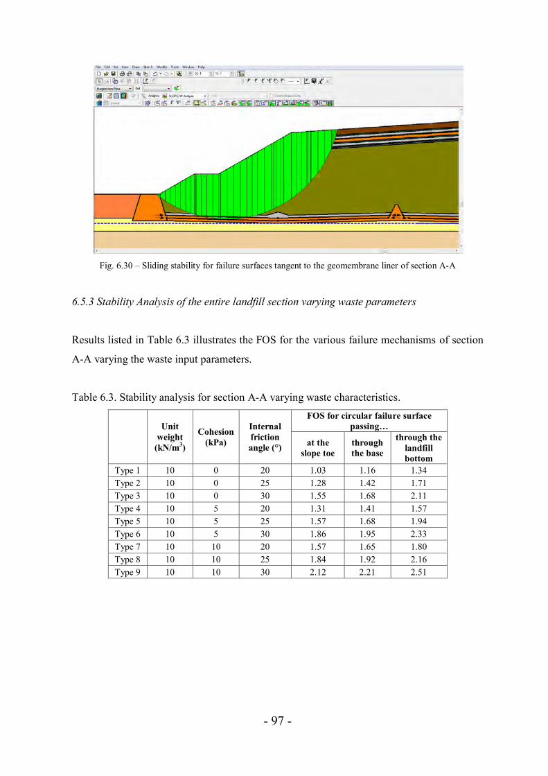
- 97 -

Fig. 6.30 – Sliding stability for failure surfaces tangent to the geomembrane liner of section A-A


Results listed in Table 6.3 illustrates the FOS for the various failure mechanisms of section

A-A varying the waste input parameters.

Table 6.3. Stability analysis for section A-A varying waste characteristics.

Unit

weight (kN/m3)

Cohesion (kPa)



at the slope toe

through the base



- 98 -

7. Calculation procedure using FEM software:

PLAXIS

7.1 Introduction

The finite element analysis has been performed using PLAXIS 2D software, drawing the

three sections of the landfill directly into the program. The analysis has been done

considering initial material and waste characteristics and waste characteristics related to the

worst cases among the different case studies examined with SLOPE/W software (i.e. lower

FOS and higher probability of failure, with “Type 1” waste parameters).

For section 2-2 and A-A the top cover barrier has been considered as a single block having a

density of 2000 Kg/m3, as indicated by a previous study (Mandato et al., 2003) conducted on

this part of S.E.S.A. landfill.

Regarding the general settings of the model, a 15 nodes per elements model with a plane

strain type of model has been chosen, because the geometry of the landfill is more or less a

uniform cross section with a corresponding stress state and loading scheme over a certain

length perpendicular to the cross section, and seismic coefficients are been inserted to

consider the earthquake effect. Standard fixities (full fixity at the base and roller condition at

the vertical sides) are been chosen as boundary conditions. An elastic-plastic model (Mohr-

Coulomb model) is selected to simulate the behavior of the materials and the input

parameters are those listed in Table 5.1; due to the impossibility to import a probability

density function into PLAXIS for these materials, some parameters are been modified in

order to not consider too restrictive conditions.

After the definition of the model geometry and material parameters the entire section is

divided into triangular elements in order to perform the finite element analysis; the entire

composition of the finite elements is called mesh. For this calculation a very fine mesh has

been chosen as definition of the global coarseness of the geometry.

Initial conditions provide initial pore water pressure (piezometric line at 5 m depth placed

inside the fine silty sand layer) configuration, paying particular attention to the boundary

conditions; all the analyzed sections must to have the right vertical boundary closed due to

- 99 -

the symmetry of the configurations which consider only an half of the section. Once that the

pore water conditions are been defined, the initial geometry has been changed to consider

the initial situations when the waste were not present.

Initial stresses are been defined by the K0-procedure: this methodology determines the initial

vertical stress σv0’ and the initial horizontal stress σh0’. These values are related by the

coefficient of lateral earth pressure K0 (σh0’ = K0 σv0’) that is defined as K0 = 1 – senφ

(Jaky’s formula) where φ is the friction angle of each material.

The calculation is done inserting a simulation of the loading of waste and top cover barrier

system into the entire landfill section, while the global safety factor has been computed by

the phi-c reduction methodology. Discussions about the obtained results are reported in the

next Chapter.

7.2 Phi-c reduction safety analysis

Phi-c reduction is the method used by PLAXIS to calculate a global factor of safety. The

program defines the FOS as a ratio between the true shear strength and the computed

minimum strength required for the equilibrium:

where c and φ are the input strength parameters and σn is the actual normal stress

component, while parameters cr and φr are reduced strength parameters that are just large

enough to maintain equilibrium. This consideration is the basis of the Phi-c reduction

method where the cohesion and the tangent of the friction angle are reduced in the same

proportion:

The reduction of the shear strength parameters in controlled by the total multiplier ∑Msf

which is increased in a step-by-step procedure (usually 100 steps are sufficient to arrive at a

state of failure) until failure occurs; the factor of safety is defined as the value of ∑Msf at

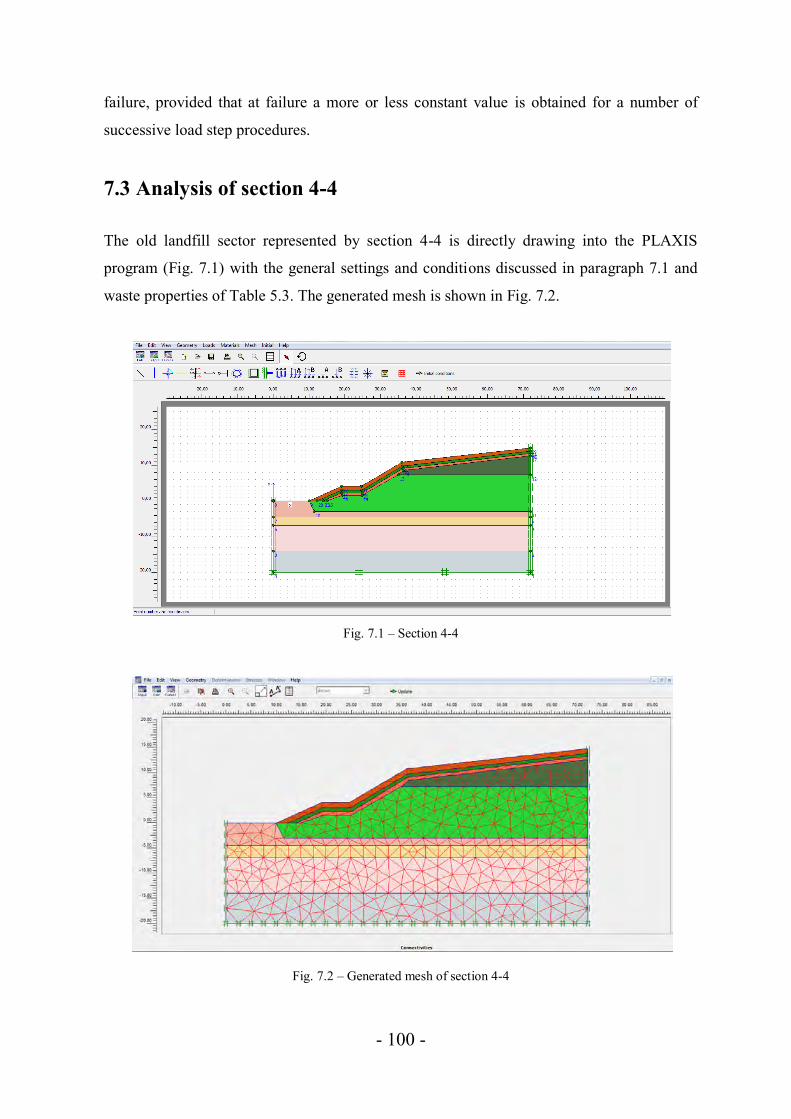
- 100 -

failure, provided that at failure a more or less constant value is obtained for a number of

successive load step procedures.


The old landfill sector represented by section 4-4 is directly drawing into the PLAXIS

program (Fig. 7.1) with the general settings and conditions discussed in paragraph 7.1 and

waste properties of Table 5.3. The generated mesh is shown in Fig. 7.2.

Fig. 7.1 – Section 4-4

Fig. 7.2 – Generated mesh of section 4-4

- 101 -

The calculated FOS results equal to 1.27; it has been evaluated also the case of different

waste input parameters (“Type 1” condition: γ = 10 kN/m3, c’ = 0 kPa, φ’ = 20°): in this case

the FOS results equal to 1.11.


Left half of section 2-2 is drawn directly into the PLAXIS program (Fig. 7.3). As previously

said, top cover barrier systems of sections 2-2 and A-A are been assumed as constant loads

of 2000 Kg/m3 (same hypothesis made by a previous slope stability analysis of the site, [20])

for the longest and almost linear part of the cover (including natural soil, compost layer,

water drainage layer, compost, compacted clay, compost, biogas captation layer, compost

and leveling layer) and 800 Kg/m3 for the part of the slope covered only by natural soil and

compost. Generated mesh with very fine coarseness is illustrated in Fig. 7.4.

Fig. 7.3 – Section 2-2

- 102 -

Fig. 7.4 – Generated mesh of section 2-2

The calculated safety factor results equal to 2.57, indicating a very good stability; using the

“Type 1” waste characteristics, FOS is reduced to 1.6.

7.5 Analysis of section A-A

Section A-A presents the same hypotheses of section 2-2. The section and the relative

generated mesh with PLAXIS are shown in Figures 7.5 and 7.6. Considering the initial

waste parameters, FOS results equal to 2.38, while inserting modified waste parameters FOS

= 1.35.

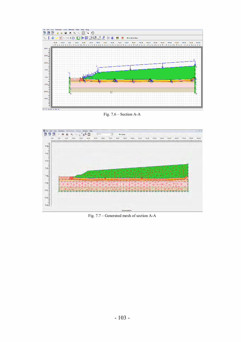
- 103 -

Fig. 7.6 – Section A-A

Fig. 7.7 – Generated mesh of section A-A

- 104 -

8. Discussion of the results

This Chapter analyzes more deeply the results obtained by the calculations with SLOPE/W

and PLAXIS softwares: the Monte Carlo approach used with SLOPE/W permits to evaluate

the results with a probabilistic point of view, while the PLAXIS program allows to observe

which are the most critical zones (top cover, bottom barrier, waste body) of the sections for

the slope stability.

Regarding the SLOPE/W program, considering the different case studied varying the input

parameters, it’s possible to obtain a probability density function for the different factors of

safety and the related probability of failure and reliability index, that are two useful indices

to evaluate the stability or the risk level of the slope. Moreover, a sensibility analysis has

been done to establish which are the most influential parameters for such possible cases.

The probability of failure is defined as the probability to obtain a safety factor less than 1.0

and is determined by counting the number of FOS below 1.0 and then taking this number as

a percentage of the total number of converged Monte Carlo trials; it’s helpful to show the

level of risk of instability for the slope under investigation.

The reliability index is defined as:

where:

- = mean of the trial factors of safety;

- = standard deviation of the trial factors of safety.

This index defines the stability by the number of standard deviations separating the mean

factor of safety from its defined value of 1.0 and can be interpreted as a method to normalize

the FOS with respect to its uncertainty level. Once that the probability distribution is known,

the reliability index can be related directly to the failure probability (Fig. 8.1).

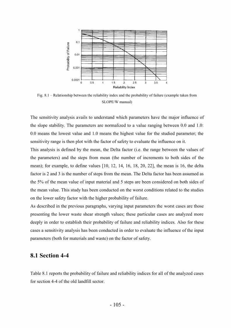
- 105 -

Fig. 8.1 – Relationship between the reliability index and the probability of failure (example taken from

SLOPE/W manual)

The sensitivity analysis avails to understand which parameters have the major influence of

the slope stability. The parameters are normalized to a value ranging between 0.0 and 1.0:

0.0 means the lowest value and 1.0 means the highest value for the studied parameter; the

sensitivity range is then plot with the factor of safety to evaluate the influence on it.

This analysis is defined by the mean, the Delta factor (i.e. the range between the values of

the parameters) and the steps from mean (the number of increments to both sides of the

mean); for example, to define values [10, 12, 14, 16, 18, 20, 22], the mean is 16, the delta

factor is 2 and 3 is the number of steps from the mean. The Delta factor has been assumed as

the 5% of the mean value of input material and 5 steps are been considered on both sides of

the mean value. This study has been conducted on the worst conditions related to the studies

on the lower safety factor with the higher probability of failure.

As described in the previous paragraphs, varying input parameters the worst cases are those

presenting the lower waste shear strength values; these particular cases are analyzed more

deeply in order to establish their probability of failure and reliability indices. Also for these

cases a sensitivity analysis has been conducted in order to evaluate the influence of the input

parameters (both for materials and waste) on the factor of safety.

8.1 Section 4-4

Table 8.1 reports the probability of failure and reliability indices for all of the analyzed cases

for section 4-4 of the old landfill sector.

- 106 -

Table 8.1. Probability of failure and reliability indices for section 4-4.

Case studies

Circular failure surface passing…

at the slope toe through the base through the landfill bottom

FOS P. of failure

Reliab. index FOS P. of

failure Reliab. index FOS P. of

failure Reliab. index

Initial case 2.02 0% 16.07 1.88 0% 13.15 2.24 0% 16.79

Type 1 (γ = 10 kN/m3, c =

0 kPa, ϕ = 20 °) 1.14 0.25% 2.64 1.16 0.1% 3.01 1.71 0% 7.87

Type 2 (γ = 10 kN/m3, c = 0 kPa,

ϕ = 25 °) 1.43 0% 5.36 1.45 0% 5.68 2.14 0% 9.49

Type 3 (γ = 10 kN/m3, c = 0 kPa,

ϕ = 30 °) 1.76 0% 7.11 1.77 0% 7.35 2.51 0% 11.92

Type 4 (γ = 10 kN/m3, c = 5 kPa,

ϕ = 20 °) 1.49 0% 8.19 1.49 0% 5.61 1.97 0% 10.57

Type 5 (γ = 10 kN/m3, c = 5 kPa,

ϕ = 25 °) 1.79 0% 9.81 1.79 0% 7.47 2.35 0% 13.48

Type 6 (γ = 10 kN/m3, c = 5 kPa,

ϕ = 30 °) 2.11 0% 10.55 2.10 0% 8.81 2.72 0% 13.38

Type 7 (γ = 10 kN/m3, c = 10 kPa,

ϕ = 20 °) 1.80 0% 10.99 1.79 0% 11.04 2.22 0% 14.79

Type 8 (γ = 10 kN/m3, c = 10 kPa,

ϕ = 25 °) 2.11 0% 12.06 2.05 0% 14.51 2.56 0% 14.97

Type 9 (γ = 10 kN/m3, c = 10 kPa,

ϕ = 30 °) 2.45 0% 15.99 2.24 0% 14.72 2.93 0% 14.63

As can be seen from the above Table, the most critical cases for section 4-4 are those

presenting a probability of failure major than 0 %, i.e. the “Type 1” cases for circular failure

surfaces passing at the toe of the slope and through the ground surface; the first case has a

FOS lower than the other case and has a higher probability of failure equal to the 0.25 %.

Fig. 8.2 shows the relationship between the probability of failure and the factor of safety for

the most critical case (FOS = 1.14, P. of failure = 0.25 % and reliability index = 2.64). This

circumstance is for a “Type 1” material properties for circular failure surface passing

through the toe of the slope.

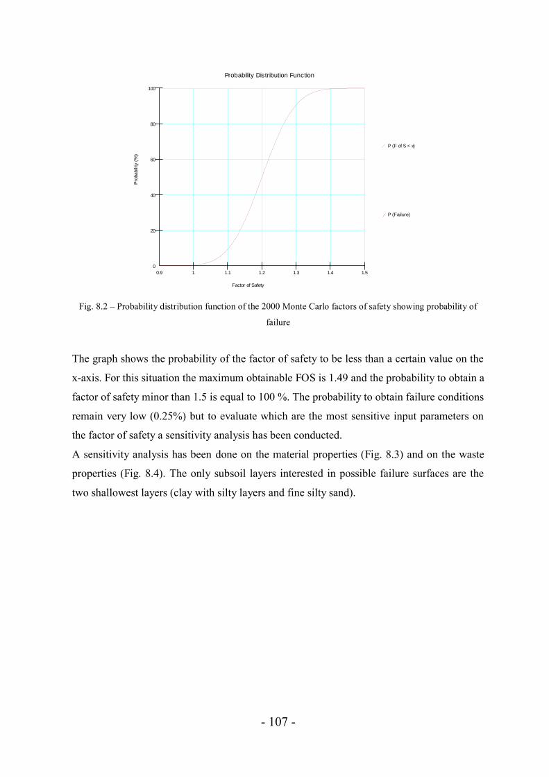
- 107 -

Fig. 8.2 – Probability distribution function of the 2000 Monte Carlo factors of safety showing probability of

failure

The graph shows the probability of the factor of safety to be less than a certain value on the

x-axis. For this situation the maximum obtainable FOS is 1.49 and the probability to obtain a

factor of safety minor than 1.5 is equal to 100 %. The probability to obtain failure conditions

remain very low (0.25%) but to evaluate which are the most sensitive input parameters on

the factor of safety a sensitivity analysis has been conducted.

A sensitivity analysis has been done on the material properties (Fig. 8.3) and on the waste

properties (Fig. 8.4). The only subsoil layers interested in possible failure surfaces are the

two shallowest layers (clay with silty layers and fine silty sand).

Probability Distribution Function

P (F of S < x)

P (Failure)

Pro

bability (

%)

Factor of Safety

0

20

40

60

80

100

0.9 1 1.1 1.2 1.3 1.4 1.5

- 108 -

Fig. 8.3 – Sensitivity analysis for material properties

From the above Figure, it’s possible to say that the compacted clay cohesion and the natural

soil cohesion have the higher positive influence on the safety factor (an increase of their

values lead to an increase of the FOS); the unit weight of compacted clay and compost have

the higher negative influence on the compute of the factor of safety.

Fig. 8.4 – Sensitivity analysis for waste properties

Figure 8.4 shows that the waste angle of internal friction presents the only positive effect on

the stability (a value of 1.0 means that for the higher values of internal friction angle the

Sensitivity Data

Material "Natural soil": Unit WeightMaterial "Natural soil": CohesionMaterial "Natural soil": PhiMaterial "Compost": Unit WeightMaterial "Compost": CohesionMaterial "Compost": PhiMaterial "Clay": Unit WeightMaterial "Clay": CohesionMaterial "Clay": PhiMaterial "Leveling layer": UnitWeightMaterial "Leveling layer": CohesionMaterial "Leveling layer": PhiMaterial "Clay w ith silty layers": UnitWeightMaterial "Clay w ith silty layers":CohesionMaterial "Clay w ith silty layers": PhiMaterial "Fine silty sand": UnitWeightMaterial "Fine silty sand": CohesionMaterial "Fine silty sand": Phi

Fa

cto

r o

f S

afe

ty

Sensitivity Range

1.13

1.132

1.134

1.136

1.138

1.14

1.142

1.144

1.146

1.148

1.15

0 0.2 0.4 0.6 0.8 1

Sensitivity Data

Material "Waste": Unit Weight

Material "Waste": Cohesion

Material "Waste": Phi

Fa

cto

r o

f S

afe

ty

Sensitivity Range

0.8

0.9

1

1.1

1.2

1.3

1.4

1.5

1.6

0 0.2 0.4 0.6 0.8 1

- 109 -

factor of safety results to have the higher values). The cohesion is set fix to 0 that is the most

precautionary value, while the variation of the unit weight doesn’t present any influence on

the FOS value.

A sensitivity analysis has been done also for the critical case of the stability of the first

slope, where a FOS = 0.99 identified a critical slip surface involving a small movement only

for soil and compost layers (Fig. 6.9a). For this particular case (the only one for this analysis

with a FOS ˂ 1.0) the probability of failure is equal to 17.4 %. The sensitivity analysis for

top barrier materials of old landfill is shown in Fig. 8.5.

Fig. 8.5 – Sensitivity analysis for top barrier material properties

Cohesion of natural soil and angle of internal friction of compost have the higher positive

influence on the FOS values, while unit weights of natural soil and compost have the higher

negative influence.

The PLAXIS program permits to identified the most critical zones of the section,

considering both initial waste parameters (FOS = 1.27, Fig 8.6) and modified waste

parameters (FOS = 1.11, Fig. 8.7).

Sensitivity Data

Material "Natural soil": Unit WeightMaterial "Natural soil": CohesionMaterial "Natural soil": PhiMaterial "Compost": Unit WeightMaterial "Compost": CohesionMaterial "Compost": PhiMaterial "Clay": Unit WeightMaterial "Clay": CohesionMaterial "Clay": PhiMaterial "Leveling layer": UnitWeightMaterial "Leveling layer": CohesionMaterial "Leveling layer": Phi

Fa

cto

r o

f S

afe

ty

Sensitivity Range

0.85

0.9

0.95

1

1.05

1.1

1.15

0 0.2 0.4 0.6 0.8 1

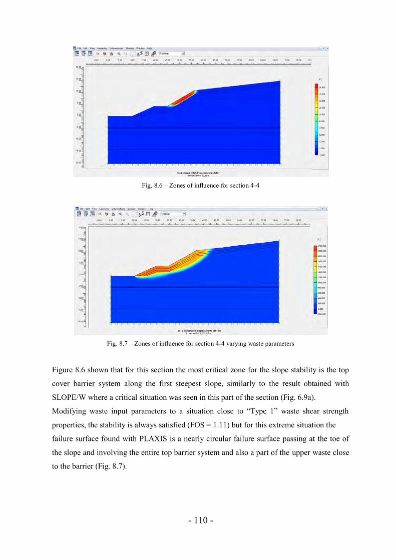
- 110 -

Fig. 8.6 – Zones of influence for section 4-4

Fig. 8.7 – Zones of influence for section 4-4 varying waste parameters

Figure 8.6 shown that for this section the most critical zone for the slope stability is the top

cover barrier system along the first steepest slope, similarly to the result obtained with

SLOPE/W where a critical situation was seen in this part of the section (Fig. 6.9a).

Modifying waste input parameters to a situation close to “Type 1” waste shear strength

properties, the stability is always satisfied (FOS = 1.11) but for this extreme situation the

failure surface found with PLAXIS is a nearly circular failure surface passing at the toe of

the slope and involving the entire top barrier system and also a part of the upper waste close

to the barrier (Fig. 8.7).

- 111 -

8.2 Section 2-2


for section 2-2.

Table 8.2. Probability of failure and reliability indices for section 2-2.

Case studies



FOS P. of failure




Initial case 1.75 0% 11.61 1.81 0% 13.34 3.05 0% 17.27

Type 1 (γ = 10 kN/m3, c =

0 kPa, ϕ = 20 °) 1.02 10.55% 1.19 1.24 0% 5.06 1.95 0% 11.65

Type 2 (γ = 10 kN/m3, c = 0 kPa,

ϕ = 25 °) 1.28 0% 4.40 1.48 0% 7.49 2.33 0% 12.62

Type 3 (γ = 10 kN/m3, c = 0 kPa,

ϕ = 30 °) 1.56 0% 6.50 1.74 0% 8.93 2.74 0% 12.88

Type 4 (γ = 10 kN/m3, c = 5 kPa,

ϕ = 20 °) 1.31 0% 5.97 1.46 0% 8.84 2.13 0% 13.85

Type 5 (γ = 10 kN/m3, c = 5 kPa,

ϕ = 25 °) 1.57 0% 8.32 1.72 0% 10.48 2.51 0% 14.30

Type 6 (γ = 10 kN/m3, c = 5 kPa,

ϕ = 30 °) 1.85 0% 9.57 1.99 0% 11.76 2.92 0% 14.99

Type 7 (γ = 10 kN/m3, c = 10 kPa, ϕ = 20 °)

1.56 0% 9.35 1.67 0% 11.77 2.31 0% 15.65

Type 8 (γ = 10 kN/m3, c = 10 kPa, ϕ = 25 °)

1.84 0% 10.95 1.93 0% 12.84 2.69 0% 15.77

Type 9 (γ = 10 kN/m3, c = 10 kPa, ϕ = 30 °)

2.14 0% 12.16 2.21 0% 13.14 3.09 0% 16.15

Waste parameters are been changed also for cases of possible sliding movements on

geosynthetic liners, but already in the worst possible case (Type 1 condition) the stability is

well respected (FOS = 1.60, P. of failure = 0% and R. index = 8.72 for sliding on geotextile

liner; FOS = 1.64, P. of failure = 0% and R. index = 9.06 for sliding on geomembrane liner).

- 112 -

The most critical case among those studied is related to Type 1 waste parameters conditions

for circular failure surface passing at the toe of the slope: in this case the safety factor is

equal to 1.02 presenting a probability of failure of 10.55% (Fig. 8.8).

A sensitivity analysis on soil and waste properties has been made in order to assess which

are the materials and parameters that have the higher (positive or negative) influence on the

factor of safety. Fig. 8.9 shows the sensitivity analysis graph for materials involved in the

failure surface (not the subsoil materials). Sensitivity analysis for waste parameters is

reported in Fig. 8.10.

Fig. 8.8 - Probability distribution function of the 2000 Monte Carlo factors of safety showing probability of

failure


P (F of S < x)

P (Failure)

Pro

ba

bili

ty (

%)

Factor of Safety

0

20

40

60

80

100

0.8 0.9 1 1.1 1.2 1.3 1.4

- 113 -


Cohesion of natural soil and clay and angle of internal friction of gravel have the higher

positive influence on the safety factor, while unit weights of gravel, compost and soil

present the higher negative influence on the calculation of the FOS.

Fig. 8.10 – Sensitivity analysis for waste properties

As expectable, also for section 2-2 the only parameter with a positive influence on the factor

of safety is the angle of internal friction of waste, but in this case the maximum obtainable

Sensitivity Data

Material "Natural soil": Unit WeightMaterial "Natural soil": CohesionMaterial "Natural soil": PhiMaterial "Compost": Unit WeightMaterial "Compost": CohesionMaterial "Compost": PhiMaterial "Clay": Unit WeightMaterial "Clay": CohesionMaterial "Clay": PhiMaterial "Leveling layer": UnitWeightMaterial "Leveling layer": CohesionMaterial "Leveling layer": PhiMaterial "Gravel": Unit WeightMaterial "Gravel": CohesionMaterial "Gravel": Phi

Fa

cto

r o

f S

afe

ty

Sensitivity Range

1.018

1.02

1.022

1.024

1.026

1.028

1.03

1.032

0 0.2 0.4 0.6 0.8 1

Sensitivity Data




Fa

cto

r o

f S

afe

ty

Sensitivity Range

0.7

0.8

0.9

1

1.1

1.2

1.3

0 0.2 0.4 0.6 0.8 1

- 114 -

safety factor is equal to less than 1.3. Figures 8.11 and 8.12 show the most critical zones for

the stability implementing PLAXIS procedure. The first case presents a FOS = 2.57,

indicating a good stability and pointing out a circular failure surface passing nearly the

landfill bottom involving a consistent part of the waste mass.

Fig. 8.11 – Zones of influence for section 2-2

Figure 8.12 shows the circular failure surface for the most critical case, varying waste

characteristics: also in this case the stability is respected (FOS = 1.6) but yet again the most

crucial zone is the part related to the first steepest slope of the section.

Fig. 8.12 – Zones of influence for section 2-2 varying waste parameters

- 115 -

8.3 Section A-A


for section A-A.

Table 8.3. Probability of failure and reliability indices for section A-A.

Case studies



FOS P. of failure




Initial case 1.75 0% 11.72 1.81 0% 12.71 2.54 0% 12.49

Type 1 (γ = 10 kN/m3, c =

0 kPa, ϕ = 20 °) 1.03 6.4% 1.41 1.16 0.05% 3.51 1.34 0% 4.99

Type 2 (γ = 10 kN/m3, c = 0 kPa,

ϕ = 25 °) 1.28 0% 4.51 1.42 0% 6.28 1.71 0% 7.55

Type 3 (γ = 10 kN/m3, c = 0 kPa,

ϕ = 30 °) 1.55 0% 6.58 1.68 0% 8.09 2.11 0% 8.97

Type 4 (γ = 10 kN/m3, c = 5 kPa,

ϕ = 20 °) 1.31 0% 5.99 1.41 0% 7.62 1.57 0% 7.95

Type 5 (γ = 10 kN/m3, c = 5 kPa,

ϕ = 25 °) 1.57 0% 8.35 1.68 0% 9.89 1.94 0% 9.80

Type 6 (γ = 10 kN/m3, c = 5 kPa,

ϕ = 30 °) 1.86 0% 9.59 1.95 0% 10.78 2.33 0% 12.85

Type 7 (γ = 10 kN/m3, c = 10 kPa, ϕ = 20 °)

1.57 0% 9.54 1.65 0% 10.91 1.80 0% 10.62

Type 8 (γ = 10 kN/m3, c = 10 kPa, ϕ = 25 °)

1.84 0% 11.42 1.92 0% 12.17 2.16 0% 11.87

Type 9 (γ = 10 kN/m3, c = 10 kPa, ϕ = 30 °)

2.12 0% 12.06 2.21 0% 13.10 2.51 0% 14.36

Type 1 waste parameters condition has been applied also to the cases of possible sliding

movements along the geosynthetic liners placed in the landfill bottom. The stability is well

respected for the case of a possible sliding both on the geotextile (FOS = 1.70, P. of failure =

0%) and on the geomembrane (FOS = 2.12, P. of failure = 0%).

Similarly to the other sections, the most critical case is related to Type 1 condition for

circular failure surface passing at the toe of the slope: in this case, FOS = 1.03 with a P. of

- 116 -

failure of 6.4 % (Fig. 8.13). A sensitivity analysis (Fig. 8.14) has been done to study which

cover materials and waste parameters have the higher influence of the calculation of the

safety factor.

Fig. 8.13 - Probability distribution function of the 2000 Monte Carlo factors of safety showing probability of

failure


Cohesion of natural soil and clay and angle of shear strength of gravel have the higher

positive effect on the FOS, while unit weight of soil, gravel and compost present the higher

negative effect on the FOS. These considerations are the same of those made for section 2-2,

due to the similar section geometry and top cover barrier system of the previous analyzed


P (F of S < x)

P (Failure)

Pro

ba

bili

ty (

%)

Factor of Safety

0

20

40

60

80

100

0.8 0.9 1 1.1 1.2 1.3 1.4

Sensitivity Data

Material "Natural soil": Unit WeightMaterial "Natural soil": CohesionMaterial "Natural soil": PhiMaterial "Compost": Unit WeightMaterial "Compost": CohesionMaterial "Compost": PhiMaterial "Clay": Unit WeightMaterial "Clay": CohesionMaterial "Clay": PhiMaterial "Leveling layer": UnitWeightMaterial "Leveling layer": CohesionMaterial "Leveling layer": PhiMaterial "Gravel": Unit WeightMaterial "Gravel": CohesionMaterial "Gravel": Phi

Fa

cto

r o

f S

afe

ty

Sensitivity Range

1.025

1.03

1.035

1.04

1.045

0 0.2 0.4 0.6 0.8 1

- 117 -

section. As for the two other sections, the only waste parameter which has a positive effect

on the factor of safety is the angle of internal friction: for this section FOS augments from

0.8 until about 1.3 (Fig. 8.15).

Fig. 8.15 - Sensitivity analysis for waste properties

PLAXIS software confirms the slope stability both considering initial conditions (FOS =

2.38) and modified waste parameters (FOS = 1.35). Fig. 8.16 shows a critical zone around

the toe of the slope and near the clay berm that will separate “Lotto 3” from the future sector

named “Lotto Ovest”. Fig. 8.17 is related to the most critical waste input properties

condition; the stability is reached but the crucial region is, also for this case, the one nearly

the higher steepest slope.

Sensitivity Data




Fa

cto

r o

f S

afe

ty

Sensitivity Range

0.7

0.8

0.9

1

1.1

1.2

1.3

0 0.2 0.4 0.6 0.8 1

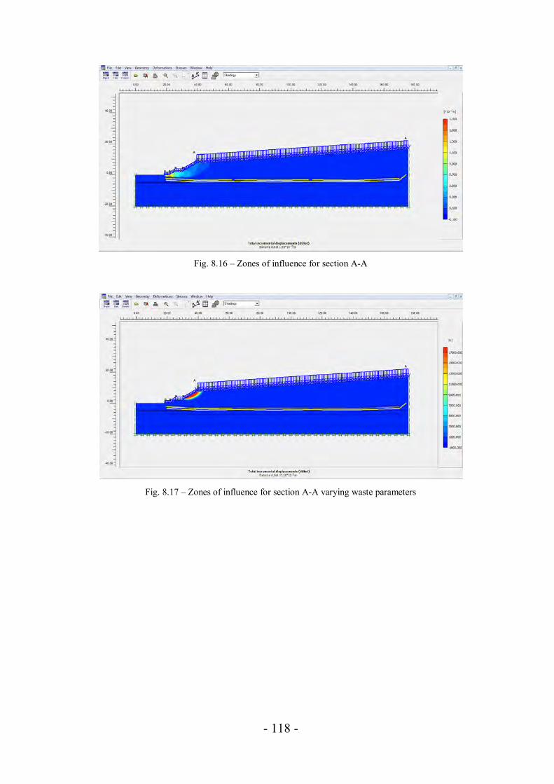
- 118 -

Fig. 8.16 – Zones of influence for section A-A

Fig. 8.17 – Zones of influence for section A-A varying waste parameters

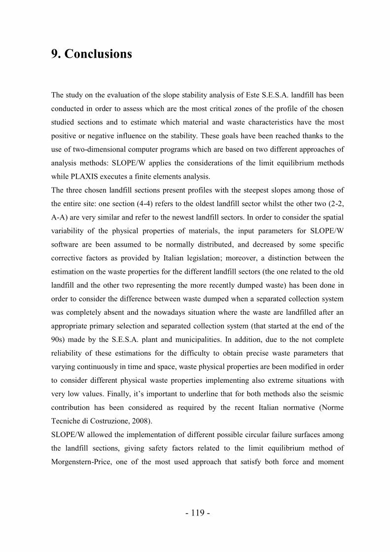
- 119 -

9. Conclusions

The study on the evaluation of the slope stability analysis of Este S.E.S.A. landfill has been

conducted in order to assess which are the most critical zones of the profile of the chosen

studied sections and to estimate which material and waste characteristics have the most

positive or negative influence on the stability. These goals have been reached thanks to the

use of two-dimensional computer programs which are based on two different approaches of

analysis methods: SLOPE/W applies the considerations of the limit equilibrium methods

while PLAXIS executes a finite elements analysis.

The three chosen landfill sections present profiles with the steepest slopes among those of

the entire site: one section (4-4) refers to the oldest landfill sector whilst the other two (2-2,

A-A) are very similar and refer to the newest landfill sectors. In order to consider the spatial

variability of the physical properties of materials, the input parameters for SLOPE/W

software are been assumed to be normally distributed, and decreased by some specific

corrective factors as provided by Italian legislation; moreover, a distinction between the

estimation on the waste properties for the different landfill sectors (the one related to the old

landfill and the other two representing the more recently dumped waste) has been done in

order to consider the difference between waste dumped when a separated collection system

was completely absent and the nowadays situation where the waste are landfilled after an

appropriate primary selection and separated collection system (that started at the end of the

90s) made by the S.E.S.A. plant and municipalities. In addition, due to the not complete

reliability of these estimations for the difficulty to obtain precise waste parameters that

varying continuously in time and space, waste physical properties are been modified in order

to consider different physical waste properties implementing also extreme situations with

very low values. Finally, it’s important to underline that for both methods also the seismic

contribution has been considered as required by the recent Italian normative (Norme

Tecniche di Costruzione, 2008).

SLOPE/W allowed the implementation of different possible circular failure surfaces among

the landfill sections, giving safety factors related to the limit equilibrium method of

Morgenstern-Price, one of the most used approach that satisfy both force and moment

- 120 -

equilibriums. Then, a sensitivity analysis along with the calculation of the probability of

failure and reliability index has been done for all of the case studied.

PLAXIS program has been used to estimate the stability to confirm if the most critical cases

and zones of the analyzed sections are the same of those found with the SLOPE/W software.

One of the two most critical cases found is the one related to possible circular failure surface

passing through the top cover barrier of the first steepest slope of the 4-4 section profile: this

situation presents the lower safety factors and the higher probability of failure, and, even if

for only one case among the 216 possible cases studied with SLOPE/W, a FOS = 0.99 has

been computed, with a failure surface involving a quantity only for natural soil and compost.

A situation for the same part of the slope that involves the entire movement of the top barrier

(soil and compost but also clay and leveling layer) presents a higher safety factor equal to

2.00. Also PLAXIS program computes a low safety factor (FOS = 1.27) for 4-4 section of

the old landfill, identifying the first steepest slope of the profile as the most critical zone

(Fig. 8.6). The sensitivity analysis shows that the material parameters presenting the higher

positive influence on the safety factor are the cohesion of natural soil and the friction angle

of compost, while the ones that negatively influence the FOS computation are the unit

weights of soil and compost. A solution to improve the stability of this part of landfill could

be the planting of more vegetations or trees.

The other critical case is the one associated to the circular failure surface that could pass at

the toe and the base of the slope: these situations present low computed factors of safety

(around 1.7 – 1.8) for all the sections if compared to the other situations studied (like failure

surface passing through the landfill bottom or tangent to the geosynthetic liners). This is

confirm also in two cases of the analysis made with PLAXIS. Material parameters that

seems to have a positive effect on the FOS calculation are the cohesions of soil and clay and

the friction angle of the gravel, while material physical properties that show a negative

influence on the safety factor are the unit weights of soil, compost and gravel. A solution to

augment the safety on this part of the landfill could be the installation of a berm of length

equal to the involved part of the base on the instability in order to improve the resisting

forces.

A suggestion to increase the reliability of the obtained results could be the investigations

with cone penetration test as method to estimate the properties of shear strength of waste,

that seems to have no negative effects on the FOS estimation; anyway, the continuous

- 121 -

variation in time and space of waste physical parameters is well known due to the different

steps of degradation processes that interested a municipal solid waste landfill.

- 122 -

10. Bibliography

[1] Abramson, Lee W., Lee, Thomas S., Sharma, Sunil, Boyce, Glenn M., 2002. Slope

Stability and Stabilization Methods (2nd ed.), New York, USA: John Wiley & Sons.

[2] Carrubba, P., 2013. Aspetti geotecnici nella realizzazione delle discariche di RSU.

Commissione di ingegneria geotecnica – Ordine degli ingegneri della provincia di Bolzano.

[3] Cheng, Y.M., Lau, C. K., 2008. Slope Stability Analysis and Stabilization: New Methods

and Insight. CRC Press, p. 15-36.

[4] Dal Prà, M., 2008. Relazione geologica e idrogeologica per il Progetto di ampliamento

della discarica SESA di RSU-RSA di Este.

[5] De Battisti, L., Drago, P., Maggio 2012. Relazione geologica (Elaborato B24) –

Elaborato adeguato alle prescrizioni approvate con la Conferenza dei Serivizi del

02/11/2011. P.A.T.I. Comuni dell’Estense. Provincia di Padova.

[6] De Marco, C., 2005. Prova Penetrometrica Statica-Prova Proctor per il terreno di

Monselice-Località Schiavonia d’Este (PD). Geodata S.a.s.

[7] Dixon, N., Russell, D., Jones, V., 2004. Engineering properties of municipal solid waste.

Department of Civil and Building Engineering, Loughborough University, Leicestershire,

UK.

[8] Duncan, J.M., 1996. State of art: limit equilibrium and finite-element analysis of slopes.

J. Geotech. Eng. 122 (7), p. 577–596.

[9] Fassett, J.B., Leonardo, G.A., Repetto, P.C., 1994. Geotechnical properties of municipal

solid waste and their use in landfill design. Waste Tech ’94, Landfill Technology Technical

Proceedings, Charleston, SC (USA).

- 123 -

[10] Favaretti, M., 2010. Environmental Geotechnics course – MSW Shear Strength.

University of Padua A.Y. 2010-2011. I.M.A.G.E. Department.

[11] Favaretti, M., 2010. Environmental Geotechnics course – Natural and artificial slopes

and general slopes stability concepts. University of Padua A.Y. 2010-2011. I.M.A.G.E.

Department.

[12] Fredlund, D. G., Krahn, J., Pufahl, D.E., 1981. The Relationship between Limit

Equilibrium Slope Stability Methods. Vol. 3, p. 409 – 416.

[13] Gharabaghi, B., Singh, M.K., Inkratas, C., Fleming, I.R., McBean, E., 2007.

Comparison of slope stability in two Brazilian municipal landfills. Waste Management 28

(2008) p. 1509-1517, Elsevier.

[14] Grisolia, M., Napoleoni, Q., Tancredi, G., 1995. The use of the triaxial tests for the

mechanical characterization of MSW. Sardinia 1995.

[15] Landva, A., Clarke, J., 1990. Geotechnics of Waste fill. Proc Symposium on

Geotechnics of Waste fills, p. 86‐103.

[16] Landva, A.O., Valsangkar, A.J., Pelkey, S.G., 2000. Lateral earth pressure at rest and

compressibility of municipal solid waste. Canadian Geotechnical Journal 37, p. 1157–1165.

[17] Look, B.G., 2007. Handbook of Geotechnical Investigation and Design Tables.

Taylor&Francis Group, London, UK.

[18] Manassero, M., Van Impe, W.F., Bouazza, A., 1996. Waste disposal and containment.

Second International Congress on Environmental Geotechnics, Osaka.

[19] Matasovic, N., Kavazanjian, E. Jr., and Anderson, R., 1998. Performance of solid waste

landfills in earthquakes, Earthquake Spectra, Issue #2, Vol. 14, p. 319-334.

- 124 -

[20] Mandato, A., Carraro, G., Avanzi, E.U., 2003. Piano di adeguamento per la discarica

di Este in base all’art. 17 del Dlgs 13 Gennaio 2003 n.36 – Verifiche geotecniche di

stabilità. S.E.S.A. S.p.a.

[21] Mandato, A., Feffin, N., Bagno, I., Piazza, E., 2008. Discarica in ampliamento.

Planimetrie stato di fatto, quote significative e destinazioni funzionali. Piano quotato area

interessata discarica (Dis. N° 5) - Nuovo impianto di selezione e valorizzazione rifiuti

urbani da raccolta differenziata con adeguamento impianto di smaltimento rifiuti urbani

non pericolosi e opere accessorie. S.E.S.A. S.p.a.

[22] Mandato, A., Feffin, N., Bagno, I., Piazza, E., 2008. Discarica in ampliamento.

Planimetria di insieme, quote significative e destinazioni funzionali delle aree (Dis. N° 7) -

Nuovo impianto di selezione e valorizzazione rifiuti urbani da raccolta differenziata con

adeguamento impianto di smaltimento rifiuti urbani non pericolosi e opere accessorie.

S.E.S.A. S.p.a.

[23] Mandato, A., Feffin, N., Bagno, I., Piazza, E., 2008. Discarica esistente. Sezioni

significative stato di fatto con stratigrafia e dettagli (Dis. N° 8a – 8b) - Nuovo impianto di

selezione e valorizzazione rifiuti urbani da raccolta differenziata con adeguamento impianto

di smaltimento rifiuti urbani non pericolosi e opere accessorie. S.E.S.A. S.p.a.

[24] Mandato, A., Feffin, N., Bagno, I., Piazza, E., 2008. Discarica in ampliamento. Sezioni

significative stato di fatto con stratigrafia e dettagli (Dis. N° 8c – 8d) - Nuovo impianto di

selezione e valorizzazione rifiuti urbani da raccolta differenziata con adeguamento impianto

di smaltimento rifiuti urbani non pericolosi e opere accessorie. S.E.S.A. S.p.a.

[25] Mandato, A., Feffin, N., Bagno, I., Piazza, E., 2008. Relazione tecnico descrittiva di

progetto (Allegato 1) – Nuovo impianto di selezione e valorizzazione rifiuti urbani da

raccolta differenziata con adeguamento impianto di smaltimento rifiuti urbani non

pericolosi e opere accessorie. S.E.S.A. S.p.a.

[26] Norme Tecniche delle Costruzioni (NTC), 2008.

- 125 -

[27] Omari, A., Bobbula, R., 2012. Slope Stability Analysis of Industrial Solid Waste

Landfills. Luleå University of Technology. Department of Civil, Environmental and Natural

Resources Engineering.

[28] Oweis, I., Khera, R., 1990. Geotechnology of Waste Management. Sevenoak, Kent,

England. Butterworth and Company Ltd.

[29] Palombi, S., 2005. Caratterizzazione geostrutturale di una discarica RSU: Analisi di

stabilità e dinamica bidimensionale – Problematiche e limitazioni connesse. Università degli

Studi di Roma “La Sapienza”.

[30] Pistolato, S., 2013. Settlement modeling of the Ca’ Rossa landfill in a post-closure

prospective. Master Thesis, ICEA Department, University of Padua.

[31] Polimeno. G., 2010. Dichiarazione ambientale EMAS – S.E.S.A. S.p.a. Impianto di Este

(Pd).

[32] Powrie, W., Beaven, R.P., 1999. Hydraulic properties of household waste and

implications for landfills. Institution of Civil Engineers Geotechnical Engineering Journal

137, p. 235–247.

[33] Quian, X., Koerner, R.M., Gray, D.H., 2002. Geotechnical aspects of landfill design

and construction.

[34] Ranjan, G., Rao, A., 2007. Basic and applied soil mechanics. Revised Second Edition.

New Age International Publishers, p. 374-376.

[35] S.E.S.A. S.p.a. Nuovo impianto di selezione e valorizzazione rifiuti urbani da raccolta

differenziata con adeguamento impianto di smaltimento rifiuti urbani non pericolosi e opere

accessorie - Piano di Sorveglianza e Controllo (P.S.C.).

- 126 -

[36] Shafer, A. L., Hargrove, J.Q., Harris, J.M., 2000. Stability analysis for Bioreactor

Landfill Operations.

[37] Stark, T.D., Eid, H.T., 1998. Performance of three-dimensional slope stability methods

in practice. J. Geotech. Geoenviron. Eng. 124 (11), p. 1049–1060.

[38] Vajirkar, M.M., 2000. Slope Stability Analysis of Class I landfills with co-disposal of

biosolids using field test data. University of Central Florida. Department of Civil and

Environmental Engineering.

[39] Van Impe, W.F., Squeglia, N., 2002. Proprietà geotecniche dei rifiuti solidi urbani.

Hevelius Editore.

[40] Yu, L., Batlle, F., 2011. A hybrid method for quasi-three dimensional slope stability

analysis in a municipal solid waste landfill. Waste Management 31 (2011), p. 2484-2496,

Elsevier.

[41] Zekkos, D.P., 2005. Evaluation of Static and Dynamic Properties of Municipal Solid-

Waste. University of California, Berkeley. Department of Civil and Environmental

Engineering.

[42] Zekkos, D., Bray, J.D., Kavazanjian, E., Matasovic, N., Rathje, E.M., Riemer, M.F.,

Stokoe II, K.H., 2006. Unit Weight of Municipal Solid Waste. Journal of Geotechnical and

Geoenvironmental Engineering. P. 1250 – 1260.

[43] PLAXIS Version 8 – http://www.plaxis.nl (Delft, The Netherlands).

[44] SLOPE/W – Slope Stability Analysis - http://www.geo-slope.com (Calgary, Canada:

Geo-Slope International).

http://www.plaxis.nl/

http://www.geo-slope.com

Geotechnical Slope Stability of the Este MSW...

Documents

Transcript of Geotechnical Slope Stability of the Este MSW...