GEOTECHNICAL ATERIALS DATABASE FOR … using M. icrosoft® Excel. 17. Key Words. embankment, ......
82
This study was sponsored by the South Carolina Department of Transportation and the Federal Highway Administration. The opinions, findings and conclusions expressed in this report are those of the authors and not necessarily those of the SCDOT or FHWA. This report does not comprise a standard, specification or regulation. Department of Civil and Environmental Engineering 300 Main Street Columbia, SC 29208 (803) 777-3614 GEOTECHNICAL MATERIALS DATABASE FOR EMBANKMENT DESIGN AND CONSTRUCTION CHARLES E. PIERCE, PH.D. SARAH L. GASSMAN, PH.D., P.E. RICHARD P. RAY, PH.D., P.E. SUBMITTED TO THE SOUTH CAROLINA DEPARTMENT OF TRANSPORTATION AND THE FEDERAL HIGHWAY ADMINISTRATION FINAL REPORT DECEMBER 1, 2011 FHWA/SCDOT Report No. FHWA-SC-11-02
Transcript of GEOTECHNICAL ATERIALS DATABASE FOR … using M. icrosoft® Excel. 17. Key Words. embankment, ......

This study was sponsored by the South Carolina Department of Transportation and the Federal Highway Administration. The opinions, findings and conclusions expressed in this report are those of the authors and not necessarily those of the SCDOT or FHWA. This report does not comprise a standard, specification or regulation.
Department of Civil and Environmental Engineering
300 Main Street Columbia, SC 29208
(803) 777-3614
GEOTECHNICAL MATERIALS DATABASE FOR EMBANKMENT DESIGN
AND CONSTRUCTION
CHARLES E. PIERCE, PH.D. SARAH L. GASSMAN, PH.D., P.E.
RICHARD P. RAY, PH.D., P.E.
SUBMITTED TO
THE SOUTH CAROLINA DEPARTMENT OF TRANSPORTATION AND
THE FEDERAL HIGHWAY ADMINISTRATION
FINAL REPORT
DECEMBER 1, 2011
FHWA/SCDOT Report No. FHWA-SC-11-02

i
Technical Report Documentation Page 1. Report No.
FHWA-SC-11-02
2. Government Accession No.
3. Recipient’s Catalog No.
4. Title and Subtitle GEOTECHNICAL MATERIALS DATABASE FOR
5. Report Date December 1, 2011
EMBANKMENT DESIGN AND CONSTRUCTION 6. Performing Organization Code
7. Author(s) C.E. Pierce, S.L. Gassman, and R.P. Ray
8. Performing Organization Report No. GT-11-01
9. Performing Organization Name and Address Department of Civil & Environmental Engineering
10. Work Unit No. (TRAIS)
University of South Carolina 300 Main Street Columbia, SC 29208
11. Contract or Grant No. SPR Project No. 670
12. Sponsoring Agency Name and Address South Carolina Department of Transportation
13. Type of Report and Period Covered
955 Park Street, P.O. Box 191 Columbia, SC 29202
14. Sponsoring Agency Code
15. Supplementary Notes Prepared in cooperation with the Federal Highway Administration. 16. Abstract This project was focused on the assimilation of engineering properties of borrow soils across the state of South Carolina. Extensive data on soils used for embankment construction were evaluated and compared within Group A (Piedmont) and Group B (Coastal Plain) soil deposits. A geotechnical materials database was constructed using three main sources of information: 1) review and synthesis of available soils information from 197 borrow pits gathered from the SCDOT Engineering Districts; 2) experimental testing of representative field samples of soils from 17 known borrow sources to determine the physical, mechanical, and chemical properties of these soils; and 3) triaxial compression test results from soil samples of existing embankments, based on a thorough review and synthesis of multiple project reports supplied by SCDOT. The geographical and geotechnical data for all of the identified borrow sources were compiled into a master spreadsheet using Microsoft® Excel.
17. Key Words embankment, borrow pit, soil compaction, shear strength, cohesion, friction angle
18. Distribution Statement No restrictions.
19. Security Classif. (of this report) Unclassified
20. Security Classif. (of this page) Unclassified
21. No. Of Pages 81
22. Price N/A
Form DOT F 1700.7 (8–72) Reproduction of completed page authorized

ii
Project Report Costs
A total of twenty five (25) copies of this final report and one hundred (100) copies of the executive summary page were printed at a cost of $400.00. The cost per unit report was $13.00 and the cost per unit summary page was $0.75.

iii
Acknowledgements
The research conducted for this report was funded by the South Carolina Department of Transportation and the Federal Highway Administration under SPR Project No. 670. Their support is greatly appreciated.
The authors wish to recognize the efforts of two graduate research assistants, Angel Ari Perez Mejia and Ke Zhou, for their assistance with the field sampling and experimental program. The following students are also acknowledged for their support and contributions throughout this project: W. Turner Allman, Eric DiFatta, Michael J. Hasek, Ryan Pierce, R. Kyle Titus, Zachary Simpson, Kenneth Wagner, Joseph R. Williamson, and Andrew Zaengle.

iv
Executive Summary
This report describes the research conducted to develop the South Carolina Department of Transportation (SCDOT) Geotechnical Materials Database (GMD) for embankment design and construction. The identification and selection of local borrow soils with established engineering properties is a critical phase in embankment design and construction. Normally, designers and contractors must conduct expensive and time-consuming geotechnical tests to determine engineering properties, or if available, use their own prior experience. The SCDOT GMD provides an electronic resource with a compilation of the specific engineering properties of potential borrow materials available throughout South Carolina. It was created using data from three sources: 1) available information from the SCDOT Engineering District offices on borrow pits that have been used for embankment construction; 2) available triaxial test data on soil samples acquired from existing embankments; and 3) comprehensive experimental program conducted using bulk samples acquired from a select number of borrow pits representing different regions of the state.
Geographical and geotechnical information were gathered from 197 borrow pits across the state of South Carolina. Geotechnical data were available for 140 of the 197 borrow pits, although in most cases, the data were limited to soil descriptions that often included USCS and/or AASHTO soil classifications. In a few cases, data were provided on particle size distribution and/or soil compaction. It was determined that 37 of the 197 borrow pits were either active or accessible, and seventeen (17) were selected for sampling and testing. Three bulk samples were collected at each borrow pit. The locations of each sampling point were based on soil maps produced using the USDA Web Soil Survey, which delineates the soil units present in each borrow pit. Tests for physical properties included visual manual identification, moisture content, specific gravity, particle size distribution, liquid limit, plastic limit, and soil classification. Tests for mechanical properties included standard Proctor compaction, direct shear, and triaxial compression, which were used to determine the most critical soil properties including maximum dry density (γd,max), optimum water content (wopt), effective friction angle, φ' and effective cohesion, c'. Tests for chemical properties included soil pH, soil resistivity, chloride content, and sulfate content. Test methods were performed according to AASHTO standard specifications, with two exceptions for chloride and sulfate contents, which were determined using USEPA test methods.
The SCDOT has created two categories of borrow soils, Group A and Group B, based on the geological environment in South Carolina. The 17 borrow pits selected for experimental studies are distributed within these two groups. Group A soils are located north and west of the Fall Line in the Blue Ridge and Piedmont physiographic geologic units. Here, most soils were formed as residuum of the underlying parent rock and therefore reflect the properties of the weathered parent material. These residual soils are often difficult to place and compact during embankment construction, and can be susceptible to erosion. Group B soils are

v
located south and east of the Fall Line in the Coastal Plain physiographic geologic unit. Coastal Plain units are identified with age and progress from the present coastline, where the youngest deposits reside, northwest toward Columbia. A diverse assortment of sands appears throughout the Coastal Plain region.
The SCDOT GMD shows that the predominant USCS and AASHTO soil classifications differ between Group A and Group B soil deposits, as expected. In general, the soils in Group B have lower fines content than those in Group A. SP-SM and SW-SM soils are common in Group B but are not found in Group A. The fines content of SM and SC soils in Group B does not exceed 32%; whereas, all but one of the SM soils in Group A has at least 35% fines. In terms of AASHTO classifications, Group B soils range from A-1 to A-4 and there are no soils with A-5 or higher classifications. In Group A, the preponderance of soil samples are classified as A-5 or higher.
The compaction characteristics are a function of soil classification. In Group A, the A-2-4 and A-4 soils have the highest γd,max (> 115 pcf in some cases) and lowest wopt required for compaction. The A-5 and A-7-5 soils have the lowest γd,max (< 100 pcf in some cases) and require the highest wopt for compaction. More than half of the Group A soils have wopt ≥ 20%. Mica was observed to be present in some of these soil samples. In Group B, the A-1 and A-2 soil groups tend to produce a higher γd,max at lower wopt than the A-3 and A-4 soil groups. All of the Group B soil samples with γd,max of at least 110 pcf are in the A-1 and A-2 soil groups. All of the Group B soils have wopt < 20%.
On average, Group A soils have higher effective friction angles than Group B soils. The results for Group A soils are in agreement with published shear strength parameters for Piedmont residual soils that indicate an average effective friction angle of 35.2° with a ± 1 standard deviation range of 29.9° < φ' < 40.5°. In Group B soils, the effective friction angles for SC, SC-SM, CL and ML soils range from 28° < φ' < 32°, which is consistent with prior SCDOT experience in the Coastal Plain. Most of the SM soils, however, were found to have higher effective friction angles ranging from 34° < φ' < 36°.
The content of this report reflects the views of the authors who are responsible for the findings and conclusions presented herein. The contents of this report do not necessarily reflect the views of the South Carolina Department of Transportation or the Federal Highway Administration. This report does not constitute a standard, specification or regulation.

vi
Table of Contents Page No.
Chapter 1 – Introduction
1.1 Problem Statement 1-1
1.2 Project Objectives 1-1
1.3 Report Organization 1-2
Chapter 2 – Background
2.1 Introduction 2-1
2.2 SCDOT Requirements for Embankment Design and Construction 2-1
2.3 South Carolina Soils 2-4
2.3.1 South Carolina Geological Regions 2-4
2.3.2 South Carolina Borrow Material Specifications 2-9
Chapter 3 – Sampling Program
3.1 Identification of Borrow Pits 3-1
3.2 Field Sampling Procedures 3-5
3.2.1 Borrow Pit Locations via GoogleTM Maps 3-5
3.2.2 General Soil Conditions 3-6
3.2.3 Borrow Pit Soil Conditions via Web Soil Survey 3-7
3.2.4 Selection of Individual Sampling Locations within Borrow Pits 3-9
3.2.5 On-Site Confirmation of Individual Sampling Locations 3-9
3.2.6 Bulk Sampling Practices 3-9
Chapter 4 – Experimental Program
4.1 Physical Properties 4-1
4.1.1 Visual-Manual Identification (ASTM D2488) 4-1
4.1.2 Moisture Content (AASHTO T 265) 4-1
4.1.3 Specific Gravity (AASHTO T 100) 4-1

vii
4.1.4 Particle Size Distribution (AASHTO T 88) 4-2
4.1.5 Liquid Limit (AASHTO T 89) 4-2
4.1.6 Plastic Limit (AASHTO T 90) 4-2
4.1.7 Soil Classification (AASHTO M 145 and ASTM D2487) 4-2
4.2 Mechanical Properties 4-3
4.2.1 Standard Proctor Compaction (AASHTO T 99) 4-3
4.2.2 Direct Shear (AASHTO T 236) 4-3
4.2.3 Triaxial Compression (AASHTO T 297) 4-3
4.3 Chemical Properties 4-5
4.3.1 pH (AASHTO T 289) 4-5
4.3.2 Resistivity (AASHTO T 288) 4-5
4.3.3 Chloride Content (USEPA Method 8225) 4-6
4.3.4 Sulfate Content (USEPA Method 8051) 4-6
Chapter 5 – Results: Soil Classification, Index Properties and
Chemical Properties
5.1 Soil Classification and Index Properties 5-1
5.1.1 Specific Gravity 5-1
5.1.2 Particle Size Distribution 5-3
5.1.3 Atterberg Limits 5-5
5.1.4 Compaction Characteristics 5-7
5.2 Chemical Properties 5-10
5.2.1 Soil pH 5-10
5.2.2 Soil Resistivity 5-13
5.2.3 Soil Chloride Content 5-15
5.2.4 Soil Sulfate Content 5-18
Chapter 6 – Results: Strength Parameters
6.1 Synthesis of Triaxial Test Data from Existing SCDOT Embankments 6-1
6.2 Strength Tests Performed at USC 6-7

viii
6.2.1 Consolidated Undrained Triaxial Tests 6-7
6.2.2 Direct Shear Test Results 6-17
Chapter 7 – Conclusions and Recommendations
7.1 Project Summary 7-1
7.2 Conclusions 7-1
7.3 Recommendations 7-3
Chapter 8 – References 8-1

ix
SI* (MODERN METRIC) CONVERSION FACTORS
APPROXIMATE CONVERSIONS TO SI UNITS APPROXIMATE CONVERSIONS FROM SI UNITS
Symbol When You Know Multiply By To Find Symbol Symbol When You
Know Multiply
By To Find Symbol
LENGTH
In
LENGTH
inches 25.4 millimeters mm mm millimeters 0.039 inches in Ft feet 0.305 meters m m meters 3.28 feet ft Yd yards 0.914 meters m m meters 1.09 yards yd Mi miles 1.61 kilometers km km kilometers 0.621 miles mi
AREA
in2
AREA
square inches 645.2 square millimeters mm2 mm2 square
millimeters 0.0016 square inches in2
ft2 square feet 0.093 square meters m2 m2 square meters 10.764 square feet ft2 yd2 square yards 0.836 square meters m2 m2 square meters 1.195 square yards yd2 Ac acres 0.405 hectares ha ha hectares 2.47 acres ac mi2 square miles 2.59 square kilometers km2 km2 square kilometers 0.386 square miles mi2
VOLUME
fl oz
VOLUME
fluid ounces 29.57 milliliters ml ml milliliters 0.034 fluid ounces fl oz Gal gallons 3.785 liters l l liters 0.264 gallons gal ft3 cubic feet 0.028 cubic meters m3 m3 cubic meters 35.71 cubic feet ft3
yd3 cubic yards 0.765 cubic meters m3 m3 cubic meters 1.307 cubic yards yd3
NOTE: Volumes greater than 1000 l shall be shown in m3
MASS
Oz
MASS
ounces 28.35 grams g g grams 0.035 ounces oz Lb pounds 0.454 kilograms kg kg kilograms 2.202 pounds lb
T Short tons (2000 lb) 0.907 megagrams
(or “metric ton”) Mg
(or “t”) Mg
(or “t”) megagrams
(or “metric ton”) 1.103 Short tons (2000 lb) T
TEMPERATURE (exact ) oF
TEMPERATURE (exact)
Fahrenheit 5(F-32)/9 Celsius 0C 0C Celsius 1.8C+32 Fahrenheit oF temperature Or (F-32)/1.8 Temperature Temperature temperature
ILLUMINATION
Fc
ILLUMINATION
foot-candles 10.76 lux lx lx lux 0.0929 foot-candles fc Fl foot-Lamberts 3.426 candela/m2 cd/m2 cd/m2 candela/m2 0.2919 foot-Lamberts fl
FORCE and PRESSURE or STRESS
Lbf
FORCE and PRESSURE or STRESS
poundforce 4.45 Newtons N N Newtons 0.225 Poundforce lbf
lbf/in2 poundforce per square inch 6.89 kilopascals kPa kPa kilopascals 0.145
Poundforce per square
inch lbf/in2
*SI is the symbol for the International System of Units. Appropriate rounding should be made to comply with Section 4 of ASTM E38.

1-1
Chapter 1 – Introduction
1.1 Problem Statement
Embankment design and construction is one of the most important phases of highway
construction. The identification and selection of local borrow soils with established engineering
properties is a critical first phase in the process. In the SCDOT Construction Manual (2004a),
Section 200.2.6 on Embankment Soil Material, it is recognized that embankment performance is,
among other factors, a function of the engineering characteristics of the embankment material,
proper placement of the embankment material in lifts, control of moisture content near optimum
during compaction, and compaction of each lift of embankment material to target density. To
ensure the structural integrity of compacted earthen embankments, the desired mechanical
properties must be achieved through appropriate materials selection and careful construction
techniques. If unsuitable soils or improper construction techniques are used, uneven settlement
or lateral displacement of the embankment can develop to a point that renders the embankment
unstable. In some cases, borrow soils might provide adequate short-term soil properties, but
their performance can deteriorate with time.
Designers and contractors often must conduct expensive and time-consuming soil and rock
testing for engineering properties, or if available, use their own prior experience. Currently,
there is a limited compilation of the specific engineering properties of potential borrow material,
including soil and rock, available throughout South Carolina for embankment construction.
Properties that influence compacted soil behavior include, but are not limited to, particle size
distribution, liquid limit (LL) and plasticity index (PI), maximum dry density (γd,max) and
optimum moisture content (wopt), and drained shear strength parameters, ' and c'. The
development of a statewide geotechnical materials database that contains engineering properties
of borrow materials would provide designers and contractors with a reliable resource on local
soils. With this resource, the time and cost efforts associated with embankment design can be
reduced significantly. It will provide a means to evaluate spatial and geological variability of
soil deposits within a particular area of the state, and most importantly, facilitate the appropriate
selection of soil shear strength parameters.
1.2 Project Objectives
There are three main research objectives for this project:
Review and synthesize readily available soils information from existing SCDOT archives
to determine the distribution of soil classification and engineering properties encountered
in Group A (Piedmont) and Group B (Coastal Plain) soil deposits, and then divide and
organize soils data according to each one of the seven Engineering Districts and 46
counties;

1-2
Collect representative field samples of soils from known borrow sources at distributed
locations within Group A and Group B soil deposits, and then determine the physical,
mechanical, and chemical properties of these soils in accordance with applicable
AASHTO, ASTM, or SC-T standard specifications; and
Compile all of the accumulated information in a Microsoft® Excel format that will serve
as a geotechnical materials database.
The purpose of the database is to provide information on soil types and soil properties in a given
area of the state, such that it can be used to guide the selection of appropriate parameters for
embankment design. The database will not be used to provide implicit prior approval of borrow
pits.
1.3 Report Organization
This report is organized into eight chapters. Chapter 2 provides background information relevant
to the project. Chapters 3 and 4 describe the field sampling and lab testing programs. Chapters 5
and 6 contain the experimental results. Chapter 7 offers conclusions and recommendations for
implementation and further studies. Chapter 8 provides the list of references. The content of
Chapters 2 through 6 is described in more detail in the following paragraphs.
Chapter 2 provides a brief overview of SCDOT requirements for soil selection and embankment
design. It also describes the geological provinces in South Carolina, with an emphasis on
residual soil formation in the Piedmont region. Lastly, it provides the borrow material
specifications for Group A and B soil deposits, along with guidance on expected soil shear
strength parameters for these two soil groups.
Chapter 3 describes the compilation of borrow pits identified across the state, and the sampling
program that was developed to obtain soils from borrow pits in Group A and B soil deposits.
The methods for identifying a representative subset of borrow pits for sampling are presented
first, followed with the field sampling procedures, which include the use of soils maps and
surveys to locate sampling points within each pit.
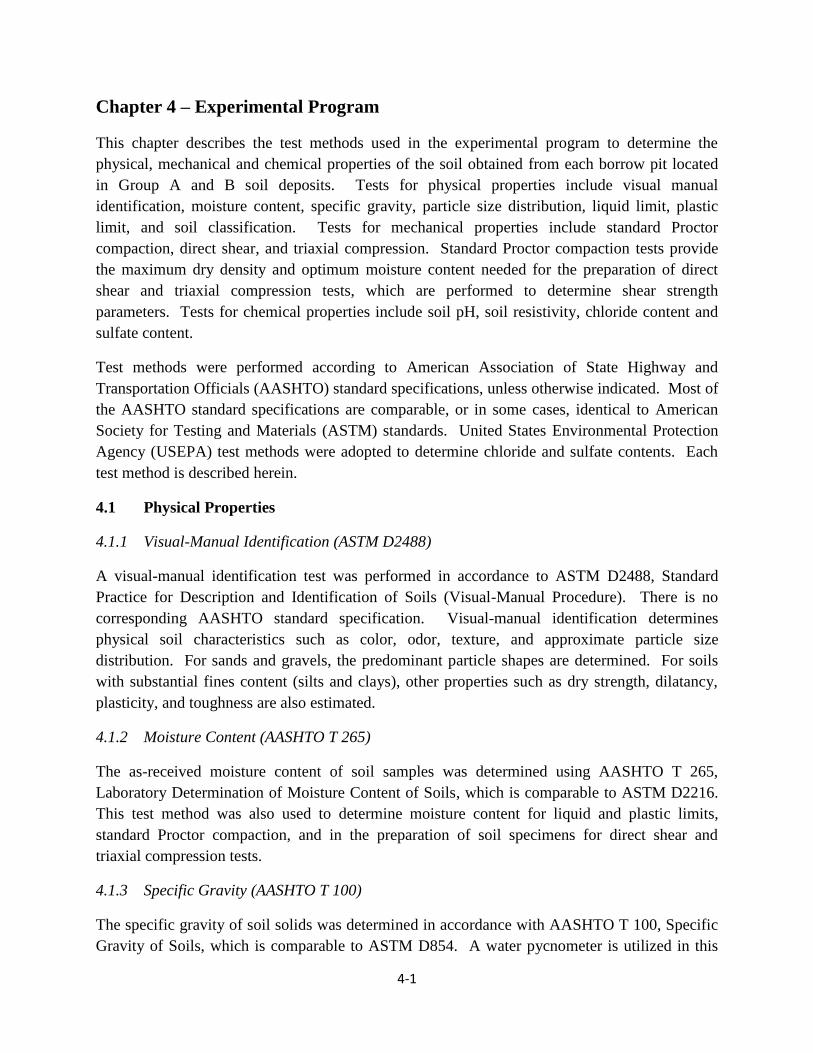
Chapter 4 describes the test methods used in the experimental program to determine the physical,
mechanical and chemical properties of the soil obtained from each borrow pit located in Group A
and B soil deposits. Tests for physical properties include visual-manual identification, moisture
content, specific gravity, particle size distribution, liquid limit, plastic limit, and soil
classification. Tests for mechanical properties include standard Proctor compaction, direct shear,
and triaxial compression. Standard Proctor compaction tests provide the maximum dry density
and optimum moisture content needed for the preparation of direct shear and triaxial
compression tests, which are performed to determine shear strength parameters. Tests for
chemical properties include soil pH, soil resistivity, chloride content and sulfate contents. Test

1-3
methods were performed according to AASHTO standard specifications unless otherwise
indicated.
Chapter 5 presents the results of the laboratory testing program performed to determine the index
properties (specific gravity, particle size distribution, liquid limit, plastic limit, maximum dry
density and optimum moisture content), soil classification according to AASHTO and USCS,
and the chemical properties (soil pH, soil resistivity, chloride content and sulfate content).
Chapter 6 presents the shear strength parameters (effective friction angle, ', and effective
cohesion, c') of Group A and B soil deposits obtained through 1) a synthesis of data provided by
the SCDOT for recent embankment projects and 2) a series of consolidated undrained static
triaxial compression tests and direct shear tests performed in the USC Geotechnical Laboratory
on soil specimens prepared from field samples of borrow pits.

2-1
Chapter 2 – Background
2.1 Introduction
Earthen embankments are common and critical elements in transportation infrastructure.
Embankments must support the pavement structure and the traffic loads that the pavement
transfers into the supporting embankment. A proper embankment design must consider:
the in-situ and as-placed properties of the fill material to be used for construction;
properties of foundation materials;
the local hydrological regime;
strength and consolidation characteristics of fill and foundation soils; and
safe slope angles for construction.
Adequate embankment performance depends on:
strength of the soil material under the embankment;
engineering characteristics of the embankment material;
proper construction of benches and transitions;
proper placement of the embankment material in lifts;
control of moisture content near optimum during compaction; and
compaction of each lift of embankment material to target density.
If unsuitable soils or improper construction techniques are used, the embankment can deform
requiring slope stabilization and pavement maintenance, like the example shown in Figure 2.1.
In extreme cases, the embankment can fail and lead to complete pavement failure, as shown in
Figure 2.2. The selection of proper shear strength parameters for the compacted soils in each
embankment design is critical.
2.2 SCDOT Requirements for Embankment Design and Construction
According to the SCDOT Geotechnical Design Manual (2010), the soil shear strength design
parameters must be locally available, cost effective, and be achievable during construction. The
selection of soil shear strength design parameters that require importing materials from outside
of the general project area should be avoided.
The method of selecting soil shear strength parameters for compacted soils will be either 1)
measured using consolidated undrained triaxial tests with pore pressure measurements, or 2)
conservatively selected based on drained soil shear strength parameters typically encountered in
South Carolina soils.

2-2
Figure 2.1. Evidence of Embankment Slope Deformation (http://mceer.buffalo.edu)
Figure 2.2. Highway Embankment Failure (http://mceer.buffalo.edu)

2-3
The selection of soil shear strength parameters for embankment design and construction depends
on whether the project is design-build, traditional design-bid-build with existing embankments,
or traditional design-bid-build on new alignment. With design-build projects, local borrow soils
must be sampled and tested for the following:
particle size distribution with wash No. 200 sieve;
liquid limit, plastic limit, and plasticity index (Atterberg Limits);
standard Proctor compaction; and
shear strength as determined from triaxial compression (TXC) consolidated undrained
(CU) tests with pore pressure measurements. Samples must be remolded and compacted
to achieve 95% relative compaction at a moisture content of -1% to +2% of the optimum
moisture content.
With traditional design-bid-build projects, the shear strength parameters are based on tests of
existing embankment soil samples, as long as similar soils are confirmed to be locally available.
With embankments on new alignments, shear strength parameters are pre-selected based on
knowledge of local soils and do not require lab testing.
The SCDOT Geotechnical Design Manual (2010) offers guidance on maximum allowable soil
shear strength parameters based on soil classification, as shown in Figure 2.3. Maximum total
shear strength for cohesive soils is limited to 1,500 psf for CL-ML soils and 2,500 psf for CL and
CH soils. However, shear strength parameters exceeding these limits can be used if the specific
source of material is identified for the project and enough material is available for construction.
Figure 2.3. Table 7-17 from the SCDOT Geotechnical Design Manual (2010)

2-4
2.3 South Carolina Soils
2.3.1 South Carolina Geological Regions
The geology of South Carolina has yielded a rich variety of minerals and igneous, metamorphic,
and sedimentary rocks. Products of weathering from these rocks as well as accumulation of
shoreline sediments form the basis for borrow materials used in construction. Products of
weathering are often found in the Piedmont region, whereas shoreline sediments have
accumulated throughout the Coastal Plain. While South Carolina is divided into these two major
geological provinces, each province may be further subdivided into more precise units as shown
in Figure 2.4.
While the variety of materials available means that engineers have many grades of materials to
work with, it presents a problem in dealing with borrow material in a consistent manner. Many
materials with specific engineering properties and behaviors may be available in one part of the
state, and not in another part. To assess the suitability of a given borrow material for an intended
engineering application, like embankment construction, a useful set of engineering properties
should be developed.
Coastal Plain units are identified with age and progress from the present coastline, where the
youngest deposits reside, northwest toward Columbia. A diverse assortment of sands appears
throughout the Coastal Plain region. Some deposits near the Orangeburg Scarp are dune sands
with fairly uniform particle distribution and varying degrees of kaolin interspersed within. Other
deposits may be intermixed with alluvial outwash (rounded gravels of varying quality) or near-
coastal deposits of calcareous (shell) materials, coquina, or organics. The various depositional
processes that have occurred throughout the Coastal Plain lead to an assortment of potential
borrow sources.
Further upland, most soils were formed as residuum of the underlying parent rock and therefore
reflect the properties of the weathered parent material. These residual soils are often difficult to
place and compact during embankment construction, and can be susceptible to erosion.
Exceptions in the Piedmont region occur where alluvial valleys have formed and deposited
gravels and sands of variable sizes, mineral content, and engineering properties. Areas where
clay is mined generally reflect the desired end use. Some clay deposits in South Carolina are
ideally suited for porcelain production, others for brick, while the remainder, if carefully
handled, can be used as structural fill. Some of these materials may require modification with
cement, lime, additional compactive effort, or other means of stabilization.
For example, in SCDOT Instructional Bulletin No. 2004-10 (2004b), it is recognized that certain
borrow soils are unsuitable for subbase unless modified with cement. As noted in this bulletin,
there are 18 counties generally located in the Piedmont region (e.g. Anderson, Greenville,
Spartanburg counties) that have experienced a hardship in readily finding satisfactory borrow
material.

2-5
Figure 2.4. Generalized Geologic Map of South Carolina (South Carolina Department of
Natural Resources, http://www.dnr.sc.gov/geology/geology.htm)
The Piedmont region is located in the eastern United States, and it is over 800 miles long,
covering a 30 mile wide stretch in Maryland to about 125 miles in North Carolina. Lengthwise,
it starts in Alabama, runs through Georgia, South and North Carolina, Virginia, Pennsylvania
and finishes in New Jersey, as shown in Figure 2.5. The topography of the Piedmont consists of
broadly rolling hills, with the hilltops forming flat ridges where major transportation routes are
placed. Streams that run through the area form narrow v-shaped valleys that are characterized by
shallow water depths and occasional shoals (Sowers 1954). The region drains in a southern and
southeastern direction towards the Atlantic Ocean.

2-6
Figure 2.5. Map of the Piedmont Region along the Eastern U.S. (Mayne and Dumas 1997)
The geologic material for the Piedmont region consists mainly of metamorphic rock intruded by
igneous rock. There are some unmetamorphosed sedimentary rock formations, but they are
rarer. White and Richardson (1987) discuss the geologic formation of rocks in the Piedmont,
along with Waisnor et al. (2001) and Sowers (1954). Metamorphic rocks in the Piedmont have
mostly metamorphosed from sedimentary rocks of the Precambrian and the lower Paleozoic age,
primarily gneisses, schists, amphibolites, phyllites, quartzite, slates and marble. The oldest rocks
are gneisses and schists that were formed during the Precambrian era from sedimentary and
igneous rocks. Theses rocks, due to the effect of heat and pressure from the metamorphic
process, have their minerals segregated into parallel bands. The bands remain parallel and
generally dip in one direction, even though the bands themselves appear twisted and swirled.
Due to volume changes and directed stresses during the last major period of deformation, joints
formed in the rock. Fluids flowed through these cracks often and deposited minerals, including
zeolite, calcite, chlorite and quartz. These joints allow for chemical weathering to occur more

2-7
easily, and in most parts of the Piedmont these joints control the degree of weathering and
resulting topography. The joint set orientations can be described as uniform or random,
depending on the area, and faults also exist throughout the region.
Soils in the Piedmont region weather in accordance to other residual soils, with a profile that
shows the most advanced weathering at the ground surface and decreasing degrees of weathering
with depth. Two example weathering profiles are illustrated in Figure 2.6. Although the
boundaries between zones are not well defined and gradual transitions between them are the
norm, four zones can be identified:
1. upper zone – completely weathered soil with well-developed soil horizons. This is the
part of the soil profile that most represents the source of borrow material;
2. intermediate structure – saprolite that retains the structure of the original rock but also
shows soil texture;
3. partly weathered zones – alternate areas of saprolite and partially weathered rock; and
4. bedrock – unaltered or slightly altered rock.
These zones have been defined from an engineering perspective, as shown in Figure 2.7. The
boundaries between zones are often not gradual, and the weathering is more advanced adjacent
to joints and mineral bands, which leads to variations in soil depth even in small areas. Climate
in the Piedmont region is particularly favorable for deep and rapid weathering with high and well
distributed rainfall throughout the region, where annual rainfall rates are on the order of 50 in.
Figure 2.6. Piedmont Weathering Profiles (Sowers 1994)

2-8
In the upper zone, these residual soils show the most advanced degree of weathering. The soil
minerals include quartz, kaolinitic clays, iron oxides and small amounts of weathered mica.
Soils in this zone tend to be classified as CL or CL-ML, and can be stiff because the in situ
moisture content is often below its plastic limit. This zone averages 3 to 5 ft in thickness, but
can be as much as 10 ft thick.
Figure 2.7. Engineering Definitions for Piedmont Weathering Zones
(Wilson and Martin 1996)
Given that the upper zone tends to be shallow, borrow soil might also come from within the
transition from the upper zone to the intermediate zone. These soils are somewhat less
weathered and are composed of quartz, kaolinitic clays and mica. Mica content in the parent
rock can be appreciable, so larger amounts of unweathered mica up to 20 or 30% can be present
in the soil. Determination of an accurate liquid limit for these soils is hindered because the soil
tends to slide in the cup instead of flow.

2-9
2.3.2 South Carolina Borrow Material Specifications
The SCDOT Geotechnical Design Manual (2010) specifies two soil groups for borrow materials,
as shown in Figure 2.8. The two groups are designated as Group A and Group B, and are
essentially divided at the geological Fall Line.
Figure 2.8. South Carolina County Map of Borrow Material Specifications (SCDOT 2010)
Group A: This group is located northwest of the Fall Line in the Blue Ridge and Piedmont
physiographic geologic units. The uppermost Blue Ridge unit contains surface soils that show a
residual soil profile, with clayey soils near the surface where weathering is more advanced,
underlain by sandy silts and silty sands. There are also colluvial deposits on the slopes. The

2-10
Piedmont unit has a similar residual soil profile, with clayey soils near the surface and sandy silts
and silty sands underneath.
SCDOT experience with borrow materials found in Group A are Piedmont residual soils
classified as micaceous clayey silts and micaceous sandy silts, clays, and silty soils in partially
drained conditions. These soils tend to have USCS classifications of either ML or MH and
typically have liquid limits greater than 30. Published laboratory shear strength testing results
for Piedmont residual soils (Sabatini 2002) indicate an average effective friction angle, φ', of
35.2° with a ± 1 standard deviation range of 29.9° < φ' < 40.5° and a conservative lower bound
of 27.3°.
Group B: This group is located south and east of the Fall Line in the Coastal Plain
physiographic geologic unit. Sedimentary soils are found at the surface and consist of
unconsolidated sand, clay, gravel, marl, cemented sands, and limestone, depending on the
location.
SCDOT experience with borrow materials found in Group B has shown that, when uniform fine
sands are used, these soils can sometimes be difficult to compact and behave similar to silts.
When these soils are encountered, caution should be used in selecting effective friction angles
since values have been shown to range from 28° < φ' < 32°.

3-1
Chapter 3 – Sampling Program
This chapter describes the sampling program that was developed to obtain soils from borrow pits
in Group A and B soil deposits from which soils have been excavated for the specific purpose of
embankment construction. Procedures were developed to identify and locate borrow pits across
the state of South Carolina and then select a representative subset for field sampling; these are
described first. Then, the field sampling procedures are presented, including the use of soils
maps and surveys, selection of sample locations within each pit, and methods for bulk sampling.
3.1 Identification of Borrow Pits
The first step in this project was to locate borrow pits from which soils have been excavated for
the specific purpose of embankment construction. The goal was to accumulate information on a
sufficient number of borrow pits across the state of South Carolina such that a representative
subset could be selected for field sampling. It was expected that the preponderance of borrow
pits would be identified within the approximate vicinity of interstate highways and/or high
population areas. Figure 3.1 is a state map that illustrates the location of each one of the 46
counties, the current corresponding SCDOT Engineering District 1 through 7, and the interstate
highway system. Borrow pits were identified within each SCDOT Engineering District, and the
results are summarized in Table 3.1.
Figure 3.1. Map of South Carolina Counties and Engineering Districts

3-2
Table 3.1. Identified Borrow Pits from the Data Provided by the SCDOT
SCDOT
District Number of Pits Active Pits
Pits with
Geotechnical
Data
Prominent
Geological Region
1 53 14 46 Carolina Sand Hills
2 8 3 2 Southern Piedmont
3 25 7 13 Blue Ridge
4 15 3 2 Southern Piedmont
5 35 5 32 Coastal Plain
6 20 5 8 Coastal Plain
7 40 0 37 Carolina Sand Hills
Total 197 37 140
Information on borrow pits was solicited from each SCDOT Engineering District. Requests
were made for pit location (address and/or GPS coordinates), size in acreage, status (active or
inactive), and owner and/or operator contact information. As shown in Table 3.1, a total of 197
borrow pits were identified. Information was also requested on soil classification and soil
properties for each pit. Geotechnical data were available for 140 of the 197 borrow pits. In
some cases, the geotechnical data were extensive and included particle size distribution and
standard Proctor compaction for multiple samples within a given pit. In most cases, however,
the data were limited to soil classification or a description of soil type. Each pit was considered
to have data if some engineering properties other than soil color were reported.
It was also reported that 37 of the borrow pits were considered to be active, or open, and the
remaining pits were considered to be closed. This information was reported from each district
and was based on their knowledge or judgement of pit status at that time. For example, the 40
borrow pits identified in District 7 were based on projects from the 1960s and were all
considered to be closed. However, owners and/or operators of all pits were contacted to verify
pit status. Of the 197 borrow pits, 107 did not have contact information and 36 others were
found to have outdated or incorrect contact information, leaving 54 borrow pits with verifiable
information. Locations of those remaining 54 borrow pits are shown in Figure 3.2.
Each one of the 197 borrow pits was named using a three-part designation convention as follows:

3-3
1. the first part indicates the SCDOT Engineering District in which the borrow pit was
located (e.g. D1 represents District 1);
2. the second part indicates the county in which the borrow pit was located (e.g. Lexington);
and
3. the third part represents the number of the borrow pit in a running series of pits within the
same district and county (e.g. 05 represents the fifth pit in that particular series).
The numerical order of pits was assigned at random. Using the example above, the pit is
designated as D1-Lexington-05.
It must be noted that the compilation of borrow pits was initiated in 2008, prior to changes in the
counties assigned to each SCDOT Engineering District. At that time, Aiken County was part of
District 1, but now it is under the management of District 7. However, in this report, all borrow
pits in Aiken County are associated with District 1. This can be seen in Figure 3.2.
Figure 3.2. Map Showing All Identified Borrow Pits from the Data Provided by SCDOT

3-4
Of the 54 borrow pits with accurate contact information, it was determined that 17 pits had been
abandoned or closed and used as sites for new construction. The other 37 pits were either active,
meaning that soil excavation was current, or accessible. The accessible pits were free from
construction and substantial vegetation such as trees, but in some cases there was low-growth
vegetative cover present, such as bushes and weeds.
Figure 3.3 marks the locations of 17 borrow pits that were selected for sampling among the 37
active or accessible pits. Six pits were located in the smaller upstate region containing Group A
soils, and eleven pits were located in the larger midlands and coastal regions containing Group B
soils. SCDOT provided one additional Group B soil sample in the vicinity of the Ace Basin, and
this sample location is designated as D6-Beaufort-04; however, this pit was not one of the
original borrow pits identified in District 6. There were no active or accessible borrow pits in
either District 5 or District 7 (not including pits in Aiken County, which were associated with
District 1 at the time). The absence of sample sites in these areas, which stretches along the I-95
corridor, is evident in Figure 3.3.
The designations of borrow pits that were selected for sampling are as follows. In Group A, the
following pits were sampled:
D2-Abbeville-01
D2-Anderson-01
D3-Oconee-01
D3-Greenville-05
D3-Anderson-05
D4-York-04
In Group B, the following pits were sampled:
D1-Richland-08
D1-Lexington-05
D1-Lexington-13
D1-Aiken-05
D1-Aiken-06
D1-Aiken-08
D1-Kershaw-01
D1-Kershaw-02
D6-Berkeley-01
D6-Dorchester-03
D6-Charleston-06
D6-Beaufort-04

3-5
Figure 3.3. Locations of Sampled Borrow Pits
3.2 Field Sampling Procedures
Field sampling was conducted over a period of time beginning in 2008 and ending in 2009. A
sampling plan was prepared in advance for each borrow pit to facilitate the acquisition of
representative soil samples at each pit. During the preparation stages, soils maps were reviewed
to determine if the soils were rather uniform or more variable within each pit. Based on those
reviews, three sampling locations were identified for each pit. A step-by-step procedure is
described in the following subsections.
3.2.1 Borrow Pit Locations via GoogleTM
Maps
Most of the borrow pits had coordinates but not physical addresses. A street address was needed
as input to obtain travel directions via GPS. Coordinates were input into GoogleTM
maps to
obtain a street address for each pit. In some cases, the pit location was confirmed at the input
coordinates through a visual assessment of the satellite image. In other cases, a pit was not

3-6
observed at the exact coordinates but was located in the vicinity. When possible, the street
address reflected the actual location of the pit; otherwise, the nearest address was recorded. For
example, the borrow pit D3-Oconee-01 was listed with coordinates of N 34° 31' 36" and W 82°
59' 30". The pit was visually located in GoogleTM
maps and the nearest address was identified as
718 Edgewood Lane, Fair Play, South Carolina, 29643.
3.2.2 General Soil Conditions
The general soil conditions expected in the area of each borrow pit were identified using a South
Carolina soils map, shown in Figure 3.4, and an AASHTO soil classification map, shown in
Figure 3.5. Both maps are based on data compiled from the USDA (United States Department of
Agriculture). The South Carolina soils map was used to assess geological soil provenience. For
example, D3-Oconee-01 is located in the southern Piedmont and the soil formation is classified
as intermediate felsic/mafic residuum. The AASHTO soil classification map provided the most
common soil types. D3-Oconee-01, for example, is located approximately where there are
prevalent A-6 and A-7 soils, depending on the exact location in that area. Information gathered
in this step was used as a guideline rather than a definitive assessment.
Figure 3.4. General Soil Map for South Carolina

3-7
Figure 3.5. AASHTO Soil Classifications of the Soils in South Carolina
3.2.3 Borrow Pit Soil Conditions via Web Soil Survey
The USDA Web Soil Survey tool was utilized to acquire more specific soils information about
each borrow pit. Web Soil Survey is a public access, online database located at
websoilsurvey.nrcs.usda.gov. This tool allows for a soil survey to be performed at any location
in the continental United States, and it can be manipulated to acquire information that includes
soil conditions and relative engineering properties. The resolution is sufficiently high to identify
the distribution of soils within the boundaries of a given borrow pit.
Figure 3.6 shows an example map produced using Web Soil Survey that delineates the soil units
present in that particular borrow pit. The area of interest (AOI) is determined by the user and, in
this case, the AOI is captured using the approximate outline of exposed soil in the pit. Table 3.2
summarizes the soil units present within the AOI. In borrow pit D3-Oconee-01, there are three
soil units present, although two of the units account for 99% of the area. The first two letters of
the soil unit represent the classification, and the third letter indicates the degree of slope at that
location. The predominant soil unit is HsC2, which represents a Hiwassee (H) sandy (s) loam;
the remaining soil units represent clay loam.

3-8
Figure 3.6. Web Soil Survey Map for Borrow Pit D3-Oconee-01 marked with Sampling
Locations 1, 2 and 3
Table 3.2. Soil Distribution in Borrow Pit D3-Oconee-01 from Web Soil Survey

3-9
3.2.4 Selection of Individual Sampling Locations within Borrow Pits
The field sampling protocol was designed to secure three diverse, representative soil samples
within each borrow pit. Sampling points were preselected on each Web Soil Survey map prior to
sampling. In cases where fewer than three distinct soil units were present at the site, at least one
sample location was marked within each soil unit. In cases where more than three distinct soil
units were present, sample locations were marked to ensure that the three samples captured the
full range of soils in that particular pit.
In the D3-Oconee-01 borrow pit, three sample locations were marked within the two major soil
units (HsC2 and LcD3), as shown in Figure 3.6. Given that the third unit (CcE3) covered a small
fraction of the exposed pit area, it was not selected for sampling. Furthermore, the soil in this
lesser unit was classified as clay loam, which was also present in one of the other two units. The
largest soil formation, Hiwassee sandy loam, was marked with two sampling points, numbered as
1 and 3. The next largest soil formation, Lloyd clay loam, was marked with one sampling point,
shown as number 2.
3.2.5 On-Site Confirmation of Individual Sampling Locations
On site, the Web Soil Survey maps were used to locate the preselected sampling points. At each
point, a visual assessment of soil color and texture was performed prior to sampling to confirm
the presence of the expected soil type. At the D3-Oconee-01 borrow pit, no changes were made
to the sampling plan, so the numbers marked in Figure 3.6 represent the location of each sample.
Sometimes at other pits, the preselected location could not be accessed or readily identified. In
these cases, a new location was selected and a visual assessment performed to determine whether
or not the soil was within the same unit as the preselected sampling location. If the soil was
deemed suitable, then a sample was acquired.
3.2.6 Bulk Sampling Practices
At each borrow pit, three bulk samples were acquired manually with the aid of a shovel, spade
and pickaxe. Samples were taken from the near-surface soil of the pit itself or, in some cases,
from existing stockpiles of soil. Prior to sampling, the uppermost foot of surface soil was first
removed and discarded, and the field sample was acquired from the subsurface. If the sample
came from a stockpile, the outer soil was removed and a field sample was extracted from the
interior of the pile. Each sample was stored and sealed in a five gallon (0.67 ft3) bucket, which
was filled completely with soil. The exact coordinates of each sampling point were recorded
using GPS. A field sampling data sheet was placed inside each bucket, and the sample numbers
were recorded on each sheet and on the exterior of the bucket.
4-1
Chapter 4 – Experimental Program
This chapter describes the test methods used in the experimental program to determine the
physical, mechanical and chemical properties of the soil obtained from each borrow pit located
in Group A and B soil deposits. Tests for physical properties include visual manual
identification, moisture content, specific gravity, particle size distribution, liquid limit, plastic
limit, and soil classification. Tests for mechanical properties include standard Proctor
compaction, direct shear, and triaxial compression. Standard Proctor compaction tests provide
the maximum dry density and optimum moisture content needed for the preparation of direct
shear and triaxial compression tests, which are performed to determine shear strength
parameters. Tests for chemical properties include soil pH, soil resistivity, chloride content and
sulfate content.
Test methods were performed according to American Association of State Highway and
Transportation Officials (AASHTO) standard specifications, unless otherwise indicated. Most of
the AASHTO standard specifications are comparable, or in some cases, identical to American
Society for Testing and Materials (ASTM) standards. United States Environmental Protection
Agency (USEPA) test methods were adopted to determine chloride and sulfate contents. Each
test method is described herein.
4.1 Physical Properties
4.1.1 Visual-Manual Identification (ASTM D2488)
A visual-manual identification test was performed in accordance to ASTM D2488, Standard
Practice for Description and Identification of Soils (Visual-Manual Procedure). There is no
corresponding AASHTO standard specification. Visual-manual identification determines
physical soil characteristics such as color, odor, texture, and approximate particle size
distribution. For sands and gravels, the predominant particle shapes are determined. For soils
with substantial fines content (silts and clays), other properties such as dry strength, dilatancy,
plasticity, and toughness are also estimated.
4.1.2 Moisture Content (AASHTO T 265)
The as-received moisture content of soil samples was determined using AASHTO T 265,
Laboratory Determination of Moisture Content of Soils, which is comparable to ASTM D2216.
This test method was also used to determine moisture content for liquid and plastic limits,
standard Proctor compaction, and in the preparation of soil specimens for direct shear and
triaxial compression tests.
4.1.3 Specific Gravity (AASHTO T 100)
The specific gravity of soil solids was determined in accordance with AASHTO T 100, Specific
Gravity of Soils, which is comparable to ASTM D854. A water pycnometer is utilized in this

4-2
test method; ASTM D5550 provides an alternative test method with a gas pycnometer, but that
method was not used in this experimental program. Specific gravity of soil solids is used in
calculations to support hydrometer analyses and standard Proctor compaction tests.
4.1.4 Particle Size Distribution (AASHTO T 88)
Particle size distribution was determined in accordance with AASHTO T 88, Particle Size
Analysis of Soils, which is comparable to ASTM D422. The distribution of particle sizes larger
than 0.075 mm (No. 200 sieve) is determined by means of mechanical separation in a sieve
analysis. The distribution of particle sizes smaller than 0.075 mm (No. 200 sieve) is determined
by means of sedimentation in a hydrometer analysis. The coarse (retained on No. 200 sieve) and
fine (passing No. 200 sieve) fractions are used in soil classification. The distribution results of
both analyses are coupled to produce a particle size distribution curve. Equivalent particle size
diameters D60, D30, and D10 are determined from each curve and used to calculate the coefficient
of uniformity, Cu, and coefficient of curvature, Cc.
4.1.5 Liquid Limit (AASHTO T 89)
The liquid limit, wLL or LL, was determined in accordance with AASHTO T 89, Determining the
Liquid Limit of Soils, which is comparable to ASTM D4318. The liquid limit test defines the
moisture content of soil at its transition to a liquid state, and it is used in soil classification. The
test method is performed on the soil fraction finer than 0.425 mm (No. 40 sieve), and the results
are influenced by the amount and mineralogical composition of the soil fraction finer than 0.075
mm (No. 200 sieve).
4.1.6 Plastic Limit (AASHTO T 90)
The plastic limit, wPL or PL, was determined in accordance with AASHTO T 90, Determining
the Plastic Limit and Plasticity Index of Soils, which is comparable to ASTM D4318. The
plastic limit test defines the moisture content of soil at its transition to a plastic state, and it is
used to determine the plasticity index, PI, for soil classification. The test method is performed
on the same soil sample that is prepared for the liquid limit test.
4.1.7 Soil Classification (AASHTO M 145 and ASTM D2487)
Soils are classified using AASHTO M 145, Classification of Soils and Soil-Aggregate Mixtures
for Highway Construction Purposes, and ASTM D2487, Standard Practice for Classification of
Soils for Engineering Purposes (Unified Soil Classification System). The two systems provide
distinct classifications, although the AASHTO and USCS classifications for each soil can often
be correlated.

4-3
4.2 Mechanical Properties
4.2.1 Standard Proctor Compaction (AASHTO T 99)
Standard Proctor compaction tests were performed in accordance with AASHTO T 99, Moisture-
Density Relations of Soils Using a 2.5-kg (5.5-lb) Rammer and a 305-mm (12-in.) Drop, which
is comparable to ASTM D698. The test method utilizes a compaction effort of 12,400 ft-lb/ft
(600 kN-m/m) per test, and multiple tests are performed at different moisture contents to
generate a compaction curve. The maximum dry density, γd,max, and optimum moisture content,
wopt, are identified from the peak of the compaction curve. Compaction tests provide
information on the physical phase relationships in soil, and the phase relations influence the
mechanical behavior. Thus, the mechanical properties of a compacted soil can be correlated with
its dry density and moisture content, and depend on whether a soil is compacted at a moisture
content that is dry of optimum (w < wopt) or wet of optimum (w > wopt).
4.2.2 Direct Shear (AASHTO T 236)
Direct shear tests were performed in accordance with AASHTO T 236, Direct Shear Test of
Soils under Consolidated Drained Conditions, which is equivalent to ASTM D3080. Tests were
performed using a strain controlled, direct shear apparatus manufactured by Wykeham Farrance.
The dimensions of the shear box are 2.5 in. × 2.5 in. (6.4 cm x 6.4 cm) square by 1.2 in. (3.1 cm)
high. Specimens were prepared in the shear box to a target density of 95% maximum standard
Proctor density at the optimum moisture content. The soil was placed in three equal lifts. Each
compacted surface was scarified before the next lift of soil was placed.
Three tests were performed on each sample at normal stresses equal to 7 psi (48.3 kPa), 14 psi
(96.5 kPa), and 21 psi (144.8 kPa). These stresses were selected to simulate the range of stresses
present in a typical highway embankment (i.e. depth range of 8.2 ft (2.5 m) to 24.3 ft (7.4 m)).
During shear, the load ring deformation, horizontal displacement and vertical displacement were
measured. The shear rate ranged from 0.0001 to 1.2 mm/min.
For each test, the relationship between the shear stress and horizontal displacement and the
relationship between horizontal displacement and vertical displacement are plotted to determine
the shear stress and normal stress at failure (defined as peak stress). Then, the shear stress and
normal stress at failure are plotted for each of the three tests to determine the slope (effective
friction angle, ') and intercept (effective cohesion, c') from the best linear fit of the data.
4.2.3 Triaxial Compression (AASHTO T 297)
Triaxial compression tests were performed according to AASHTO T 297, Consolidated
Undrained Triaxial Compression Test on Cohesive Soils, which is equivalent to ASTM D4767.
The GDS Electromechanical Dynamic Triaxial Testing System (DYNTTS) used for these tests is
shown in Figure 4.1 and was recently acquired by the Department of Civil and Environmental

4-4
Engineering in November 2010. It is a software-driven system that includes a triaxial cell
capable of providing a confining pressure up to 1 MPa, a digital processor for controlling cell
pressure, and a digital processor for controlling back pressure. The digital processors maintain
pressures to within 1 kPa. The unit is equipped with an analog pore pressure transducer and an
analog load cell transducer. The displacement is digitally-controlled through an encoder in a
stepper motor. The system has a maximum axial load capacity of 10 kN.
Specimens for triaxial testing were prepared from the soils obtained from the borrow pits across
the state. Specimens were compacted to a target of 95% maximum standard Proctor density at
optimum moisture content. The specimens were 2.0 in. (50.1 mm) in diameter and 4.0 in. (101.6
mm) in height. The corresponding height-to-diameter ratio of the specimens was H/D = 2. Two
specimen preparation methods were used. Soils with some cohesion (i.e. CL, ML) were
compacted in a standard Proctor mold per Section 4.2.1 at optimum moisture content, extracted
from the mold, and trimmed to size. Cohesionless soils (i.e. SP) were prepared inside a 2.0 in.
(50.1 mm) diameter split mold. The soil was placed in thin lifts and tamped into place to achieve
the target density. Each compacted surface was scarified before the next lift of soil was placed.
Following sample preparation, samples were saturated in the triaxial cell using a two step
process: 1) primary saturation in which specimens were flushed with de-aired water and 2) back
pressure saturation by applying a back pressure on the specimen to drive water into the specimen
and force the entrapped air into aqueous solution. The degree of saturation was found by a B-
value check using a cell pressure increment of 25 kPa. Once a satisfactory B-value was
achieved, the specimens were isotropically consolidated to 48, 96, or 144 kPa (1, 2, or 4 ksf).
After consolidation, specimens were sheared undrained in triaxial compression under strain
controlled conditions. The rate of axial strain was selected based on AASHTO T 297 (ASTM
D4767) and is a function of specimen permeability. Pore pressures were measured during
shearing.
For each test, the relationships between the principal stress difference and axial strain and the
excess pore pressure and axial strain are plotted. These data are also used to plot the stress path
in q-p space for each test. The effective friction angle, ', and the effective cohesion, c', are
determined from the slope, ψ, and intercept, a, of the linear portion of the stress path using the
following relationships: c'=a/cos ' and tan ψ=sin '.

4-5
Figure 4.1. GDS Electromechanical Dynamic Triaxial Testing System (DYNTTS) in the
Department of Civil and Environmental Engineering Advanced Geotechnical Laboratory.
4.3 Chemical Properties
4.3.1 pH (AASHTO T 289)
pH of the soil samples was determined in accordance with AASHTO T 289, Determining pH of
Soil for Use in Corrosion Testing. ASTM D4972 provides another test method that covers the
measurement of pH for uses other than corrosion testing. The test measures the concentration of
H+ ions in a soil sample to determine its degree of acidity or alkalinity.
4.3.2 Resistivity (AASHTO T 288)
The minimum electrical soil resistivity was determined in accordance with AASHTO T 288,
Determining Minimum Laboratory Soil Resistivity, which is similar to ASTM G187. These test
methods employ a two-electrode soil box to accommodate lab bench-scale tests. Soil resistivity
is a function of moisture content, and multiple tests are performed at different moisture contents

4-6
to determine the minimum resistivity. The corrosion potential of a soil can be correlated with its
minimum electrical resistivity, which corresponds to its maximum electrical conductivity.
4.3.3 Chloride Content (USEPA Method 8225)
The chloride content of soil samples was determined using an adaptation of USEPA Method
8225, Silver Nitrate Buret Titration Method for Chloride. This method was compared to
AASHTO T 291, Determining Water-Soluble Chloride Ion Content in Soil, and it was deemed to
be similar to AASHTO Method A. The differences in test procedures are confined to sample
preparation and chemical requirements. The USEPA method was found to be acceptable for use
in this investigation, and this change was approved by the SCDOT.
In this test method, silver nitrate is titrated into the soil sample until a specific color change is
noted. The amount of silver nitrate required to change color is correlated to the chloride content.
Results are reported as chloride content in mg/L.
4.3.4 Sulfate Content (USEPA Method 8051)
Like chloride content, a USEPA method was also approved and adopted for determining sulfate
content of soil samples. USEPA Method 8051, SulfaVer 4 Method for Sulfate, was found to be
similar to Method B of AASHTO T 290, Determining Water-Soluble Sulfate Ion Content in Soil,
which involves forming a precipitate of barium sulfate. The main differences are with sample
preparation, the wavelength required to measure turbidity and the provenience of chemical
compounds to provoke the reaction. Results are reported as sulfate content in parts per million
(ppm).

5-1
Chapter 5 – Results: Soil Classification, Index Properties and Chemical
Properties
This chapter presents the results of the laboratory testing program performed to determine the
properties of the soils obtained from each borrow pit located in Group A and B soil deposits.
Results of tests performed to determine the index properties (specific gravity, particle size
distribution, liquid limit, plastic limit, maximum dry density and optimum moisture content) are
presented first and used to classify the soils according to AASHTO and USCS. These results are
followed by the environmental properties determined from the chemical tests (soil pH, soil
resistivity, chloride content and sulfate content). Results of the strength tests will be presented in
Chapter 6.
5.1 Soil Classification and Index Properties
5.1.1 Specific Gravity
Figures 5.1 and 5.2 illustrate the specific gravity of soil solids, Gs, measured from each bucket
sample of each borrow pit located in Group A and Group B soil deposits, respectively. In a
given soil sample, Gs depends on the mineralogical composition and organic content. Most
inorganic soils contain a mixture of minerals such that the composite Gs commonly ranges from
2.50 to 2.80. Table 5.1 lists common soils minerals and their values of specific gravity. Quartz
and feldspars are common minerals in gravels, sands, and non-plastic silts. Kaolinite, illite, and
montmorillonite are the most common clay minerals. Table 5.1 shows that the Gs for clay
minerals can be lower and more variable than non-clay minerals, such that Gs for soils containing
significant amounts of clay minerals can depend on the distribution of mineral types.
Table 5.1. Values of Specific Gravity for Common Soil Minerals
Mineral Specific Gravity, Gs
Quartz 2.65
Orthoclase Feldspar 2.57
Plagioclase Feldspar 2.62 - 2.76
Muscovite Mica 2.76 - 3.10
Biotite Mica 2.80 - 3.20
Kaolinite 2.16 - 2.68
Illite 2.65
Montmorillonite 1.70 - 2.00
Chlorite 2.60 - 3.30
Halloysite 2.53

5-2
Values of Gs for soils from borrow pits in South Carolina fall well within the common range of
2.50 to 2.80. No sample falls below a Gs of 2.50; the lowest measured Gs is 2.53 from D6-
Charleston-06. There are four samples that exceed 2.80. One of the samples is from D2-
Abbeville-01, where a Gs of 2.83 from soil in Bucket Sample 2 is noticeably higher than Gs of
2.64 and 2.67 measured from the other two bucket samples. The higher value of Gs suggests that
the mineralogical composition of soil at the location corresponding to Bucket Sample 2 is
sufficiently different from soil at the other two sampling locations. All three soil samples taken
from D1-Richland-08 contained solids with Gs ranging from 2.83 to 2.89. As expected, some of
the borrow pits, like D1-Richland-08, had less variation in Gs than other pits, like D2-Abbeville-
01. Borrow pits with soil samples that varied more than a tenth (Gs ± 0.1) include D3-Oconee-
01, D6-Charleston-06, and D6-Berkeley-01. It should be noted that these observations are based
on a limited number of three samples acquired at each pit.
Figure 5.1. Specific Gravity, Gs, of Group A Soils
2.55
2.6
2.65
2.7
2.75
2.8
2.85
Spec
ific
Gra
vity
Sample 1
Sample 2
Sample 3

5-3
Figure 5.2. Specific Gravity, Gs, of Group B Soils
5.1.2 Particle Size Distribution
Table 5.2 summarizes the USCS and AASHTO soil classifications for each bucket sample from
borrow pits located in Group A. Soil classifications are based on the results of sieve and
hydrometer analyses to determine particle size distribution and liquid and plastic limit tests to
determine plasticity. The fines content, liquid limit (LL), and plasticity index (PI) are provided
for each soil sample.
A review of the soil classifications shows that silty sands, SM, are prevalent and account for 10
of the 18 soil samples. Each borrow pit has at least one SM soil sample, except for D3-Oconee-
01. The next most common soils are high plasticity silts, MH, which are also present in all but
one borrow pit. The pit without SM soils, D3-Oconee-01, is also the singular pit where clay
(CH) soils were classified. It should be noted that all soils contain a mixture of coarse and fine
grains, as the fines content illustrates in Table 5.2. The fines content ranges from 21% to 68%;
furthermore, 13 of the 18 soil samples have fines content of 50% ± 10%. This suggests that
2.5
2.55
2.6
2.65
2.7
2.75
2.8
2.85
2.9Sp
ecif
ic G
ravi
tySample 1
Sample 2
Sample 3

5-4
some, but not all, of the SM and MH soils should have comparable mechanical properties. In
fact, the AASHTO soil classifications reflect some of the similarities between SM, MH, and CH
soils. There are 11 A-7-5 and A-7-6 soils classified in five of the six borrow pits. D4-York-04 is
the lone exception, where the fines content tends to be lower than in the other pits such that A-2-
4 and A-4 soils are present.
Table 5.2 Soil Classification for Borrow Pits in Group A
Borrow Pit No. Soil Classification Fines Content
(% < 75 μm) LL1 PI1
USCS AASHTO
D4-York-04
1 SM A-2-4 21 NP NP
2 SM A-4 40 NP NP
3 SM A-4 37 NP NP
D2-Anderson-01
1 MH A-7-5 53 54 18
2 SM A-7-5 46 55 24
3 ML A-7-6 50 42 13
D3-Anderson-05
1 MH A-7-5 53 55 13
2 SM A-7-6 46 41 16
3 SM A-5 44 48 10
D2-Abbeville-01
1 SM A-7-6 36 45 17
2 MH A-7-5 68 58 21
3 SM A-2-4 35 38 1
D3-Greenville-05
1 SM A-5 48 44 5
2 MH A-7-5 60 53 22
3 SM A-4 41 NP NP
D3-Oconee-01
1 CH A-7-6 58 52 27
2 MH A-7-5 53 72 23
3 CH A-7-6 57 65 42 1NP means non-plastic.
Table 5.3 summarizes the USCS and AASHTO soil classifications for each bucket sample from
borrow pits located in Group B. In general, the soils in Group B have lower fines content than
those in Group A, and the soil classifications differ accordingly. SP-SM and SW-SM soils are
found in 11 of the 21 samples. By definition, these soils must contain between 5% and 12%
fines. There are six SM and SC soils, but the fines content does not exceed 32%; whereas, all
but one of the SM soils in Group A has at least 35% fines. The difference in fines content is also
reflected in the distribution of AASHTO soil classifications. In Group B, the soils range from A-

5-5
1 to A-4 and there are no soils with A-5 or higher classifications. In Group A, 13 of the 18 soil
samples are classified as A-5 or higher.
Table 5.3 Soil Classification for Borrow Pits in Group B
Borrow Pit No. Soil Classification Fines Content
(% < 75 μm) LL1 PI1
USCS AASHTO
D1-Lexington-05
1 SC A-2-6 18 31 12
2 SM A-2-4 21 NP NP
3 SC A-2-7 28 49 28
D1-Lexington-13
1 SW-SM A-1-b 6 NP NP
2 SW-SM A-1-b 7 NP NP
3 SW-SM A-1-b 8 NP NP
D1-Richland-08
1 ML A-4 75 31 7
2 ML A-4 88 35 1
3 CL-ML A-4 52 17 4
D1-Kershaw-02 2 SW-SM A-2-4 12 NP NP
3 SM A-2-4 29 NP NP
D1-Aiken-05
1 SP A-3 3 NP NP
2 SP-SM A-3 6 NP NP
3 SP-SM A-2-4 12 NP NP
D6-Charleston-06
1 SM A-2-4 20 NP NP
2 SP-SM A-3 7 NP NP
3 SP-SM A-3 8 NP NP
D6-Berkeley-01
1 SP-SM A-2-4 11 NP NP
2 SM A-2-4 32 NP NP
3 SP-SM A-3 10 NP NP
D6-Dorchester-03 1 SP-SM A-2-4 12 NP NP 1NP means non-plastic.
5.1.3 Atterberg Limits
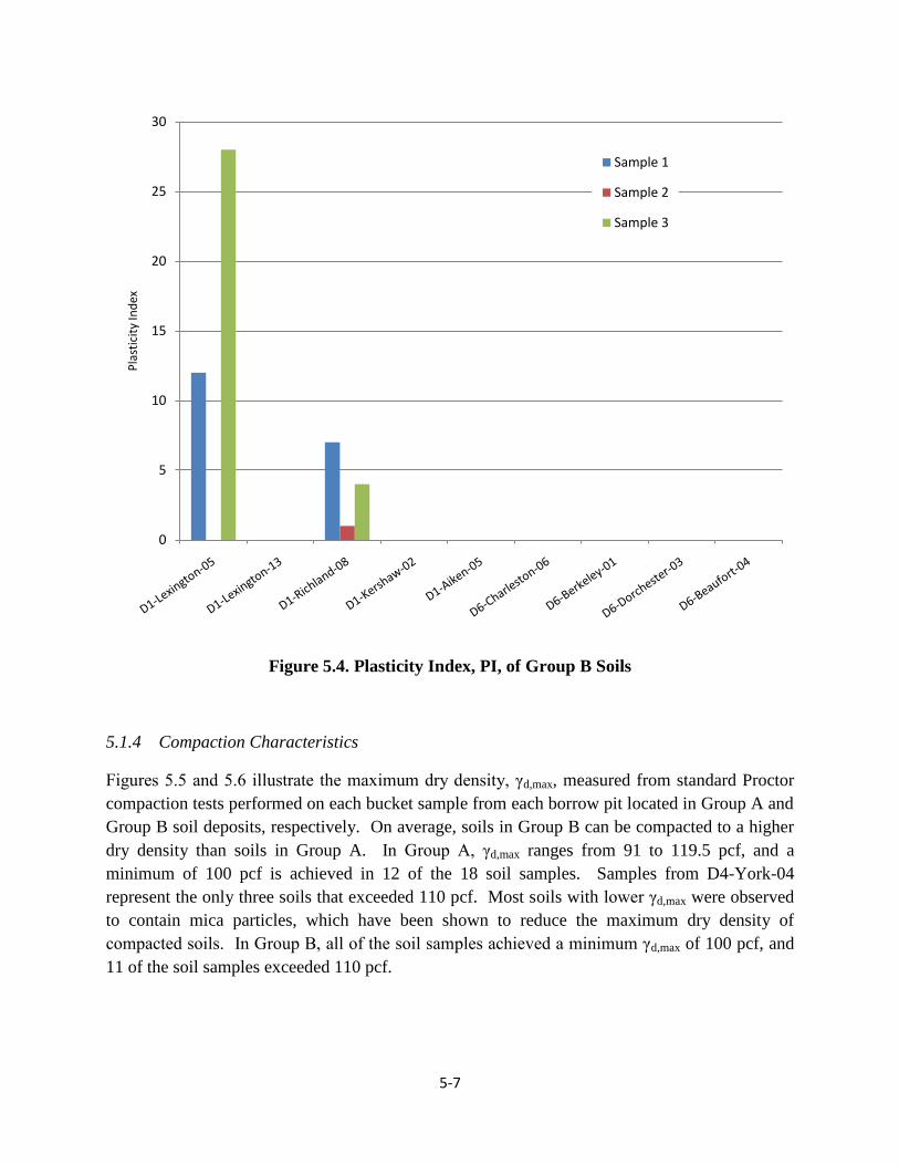
Figures 5.3 and 5.4 illustrate the plasticity index, PI, measured from each bucket sample of each
borrow pit located in Group A and Group B soil deposits, respectively. Given the geographical
and geological distinctions of each soil group, it is expected that Group A soils would have some
measurable plasticity and that Group B soils would not, except for soils within the Fall Zone
close to the division of Group A and B soils. Figure 5.3 shows that most soil samples have a PI

5-6
between 10 and 25, with a few exceptions. Soil samples collected from D4-York-04 were
determined to be non-plastic. The highest PI of 42 was measured from soil in D3-Oconee-01. It
is also observed that some borrow pits with more variable PI measurements, such as D3-Oconee-
01 and D2-Abbeville-01, also had more variable Gs measurements, as discussed in the prior
section. These correlations suggest that the differences in specific gravity and plasticity are a
function of changes in the amount and/or type of clay minerals present in the soil samples. For
Group B soils, Figure 5.4 shows that, except for two borrow pits, the fines content is limited
and/or was determined to be non-plastic. The two borrow pits containing soils with some
measureable plasticity are located in Lexington and Richland counties within the Fall Zone.
Figure 5.3. Plasticity Index, PI, of Group A Soils
0
5
10
15
20
25
30
35
40
45
D4-York-04 D2-Anderson-01 D3-Anderson-05 D2-Abbeville-01 D3-Greenville-05 D3-Oconee-01
Pla
stic
ity
Ind
ex
Sample 1
Sample 2
Sample 3
5-7
Figure 5.4. Plasticity Index, PI, of Group B Soils
5.1.4 Compaction Characteristics
Figures 5.5 and 5.6 illustrate the maximum dry density, γd,max, measured from standard Proctor
compaction tests performed on each bucket sample from each borrow pit located in Group A and
Group B soil deposits, respectively. On average, soils in Group B can be compacted to a higher
dry density than soils in Group A. In Group A, γd,max ranges from 91 to 119.5 pcf, and a
minimum of 100 pcf is achieved in 12 of the 18 soil samples. Samples from D4-York-04
represent the only three soils that exceeded 110 pcf. Most soils with lower γd,max were observed
to contain mica particles, which have been shown to reduce the maximum dry density of
compacted soils. In Group B, all of the soil samples achieved a minimum γd,max of 100 pcf, and
11 of the soil samples exceeded 110 pcf.
0
5
10
15
20
25
30P
last
icit
y In
dex
Sample 1
Sample 2
Sample 3

5-8
Figure 5.5. Maximum Dry Density of Group A Soils
Figure 5.6. Maximum Dry Density of Group B Soils
80
85
90
95
100
105
110
115
120
125
130M
axim
um
Dry
Den
sity
, pcf
Sample 1
Sample 2
Sample 3
80
85
90
95
100
105
110
115
120
125
130
Max
imu
m D
ry D
ensi
ty, p
cf
Sample 1
Sample 2
Sample 3
Composite Sample

5-9
Tables 5.4 and 5.5 compare the compaction characteristics within each AASHTO soil
classification present in Group A and Group B soil deposits, respectively.
In Group A, the A-2-4 and A-4 soils have the highest γd,max and lowest wopt required for
compaction. There is one exception in D3-Greenville-05, where mica was observed in the soil
samples. The A-7-6 soils have the next highest γd,max, with values ranging between 102 and 110
pcf. The A-5 and A-7-5 soils have the lowest γd,max and require the highest wopt for compaction.
Mica was observed to be present in some of these soil samples.
In Group B, the A-1 and A-2 soil groups tend to produce a higher γd,max at lower wopt than the A-
3 and A-4 soil groups. All of the Group B soil samples with γd,max of at least 110 pcf are in the
A-1 and A-2 soil groups. There are also noticeable differences in the wopt required for
compaction. All of the A-1 and A-2 soils, except one, have wopt ≤ 14%. Conversely, all of the
A-3 and A-4 soils, except one, have wopt ≥ 14%. It should be noted that all of the Group B soils
have wopt < 20%; whereas, 11 of the 18 Group A soils have wopt ≥ 20%.
Table 5.4 Compaction Characteristics of Group A Soils
AASHTO Soil
Classification
Borrow Pit and Bucket
Sample
Nos.
Gs Standard Proctor Compaction
γd max (pcf) wopt (%)
A-2-4 D4-York-04-B1 2.59 119.5 11
D2-Abbeville-01-B3 2.64 110 14
A-4
D4-York-04-B2 2.63 114 15.4
D4-York-04-B3 2.61 116 13.5
D3-Greenville-05-B3 2.75 93 20
A-5 D3-Anderson-05-B3 2.80 99.5 23
D3-Greenville-05-B1 2.76 98 23
A-7-5
D2-Anderson-01-B1 2.74 96.8 24.1
D2-Anderson-01-B2 2.69 103.9 22
D3-Anderson-05-B1 2.79 99 23
D2-Abbeville-01-B2 2.83 91 28
D3-Greenville-05-B2 2.74 100 23
D3-Oconee-01-B2 2.63 102.5 22.5
A-7-6
D2-Anderson-01-B3 2.71 103.5 19
D3-Anderson-05-B2 2.80 106.5 20
D2-Abbeville-01-B1 2.67 109.6 15
D3-Oconee-01-B1 2.75 102.5 23.5
D3-Oconee-01-B3 2.62 106 19

5-10
Table 5.5 Compaction Characteristics of Group B Soils
AASHTO Soil
Classification
Borrow Pit and Bucket
Sample
Nos.
Gs Standard Proctor Compaction
γd max (pcf) wopt (%)
A-1-b
D1-Lexington-13-B1 2.69 122 10.5
D1-Lexington-13-B2 2.71 122 10.5
D1-Lexington-13-B3 2.73 122 10.5
A-2-4
D1-Lexington-05-B2 2.67 122 11
D1-Kershaw-02-B2 2.74 101 14
D1-Kershaw-02-B3 2.75 111 14
D1-Aiken-05-B3 2.67 111.4 12
D6-Charleston-06-B1 2.53 106 16.5
D6-Berkeley-01-B1 2.57 105.2 12.5
D6-Berkeley-01-B2 2.54 113.4 12.3
D6-Dorchester-03-B1 2.71 107 12
A-2-6 D1-Lexington-05-B1 2.76 122 13
A-2-7 D1-Lexington-05-B3 2.74 116 12.5
A-3
D1-Aiken-05-B1 2.71 99.9 18.2
D1-Aiken-05-B2 2.66 102.3 16
D6-Charleston-06-B2 2.61 102 16
D6-Charleston-06-B3 2.64 108.4 12.6
D6-Berkeley-01-B3 2.67 103.8 17.5
A-4
D1-Richland-08-B1 2.86 106 17
D1-Richland-08-B2 2.89 109.5 14.7
D1-Richland-08-B3 2.83 109.5 14.7
5.2 Chemical Properties
5.2.1 Soil pH
Figures 5.7 and 5.8 illustrate the soil pH measured from each bucket sample of each borrow pit
located in Group A and Group B soil deposits, respectively. Table 5.6 provides a summary of
pH values for all measurements.
Soil pH is a function of soil deposition and geographic location, which in turns impacts the
presence and thickness of soil horizons within soil deposits. In general, soil pH can range from
2.8 to 10.0. However, most soils in the southeastern U.S. tend to be acidic. With the exception
of four samples, soils from borrow pits across South Carolina range from very strongly acid to

5-11
slightly acid, as shown in Table 5.6. The four samples with pH of neutral to moderately alkaline
are from borrow pits in Kershaw (Group B) and York (Group A) counties. Even though these
pits represent two different soil groups, the pits are relatively close to each other and are just
separated by Lancaster County. None of the soil samples have pH on the most extreme ends of
the acid-alkaline scale.
pH of soils within a borrow pit can be quite consistent, as shown in Figure 5.7 for D3-
Greenville-05 and D3-Oconee-01. However in most cases shown in Figures 5.7 and 5.8, the
measured pH values are variable, which is expected given the natural soil variation expected at a
given site. For each borrow pit sampled, the difference in maximum and minimum pH was ≤ 1
except for D4-York-04 (2.1 difference), D2-Anderson-01 (1.1 difference), and D6-Berkeley-01
(1.3 difference).
Figure 5.7. Soil pH for Group A Soils
7.9
55.1
4.7
6.1
6.4
6.8
4.9
5.5
5.1
5.9
6.5
5.8
5
5.4 5.4
5.9
5.4
3
4
5
6
7
8
9
D4-York-04 D3-Greenville-05 D3-Anderson-05 D2-Abbeville-01 D3-Oconee-01 D2-Anderson-01
Sample 1
Sample 2
Sample 3
Soil
pH

5-12
Figure 5.8. Soil pH for Group B Soils
Table 5.6. Description of pH measurements for Group A and B Soils
Description (Soil
Survey Division 1993) pH Range
No. of Borrow Pit Samples
Group A Group B
Ultra acid < 3.5 --- ---
Extremely acid 3.5 - 4.4 --- ---
Very strongly acid 4.5 - 5.0 4 4
Strongly acid 5.1 - 5.5 6 3
Moderately acid 5.6 - 6.0 3 5
Slightly acid 6.1 - 6.5 3 3
Neutral 6.6 - 7.3 1 1
Slightly alkaline 7.4 - 7.8 --- 1
Moderately alkaline 7.9 - 8.4 1 ---
Strongly alkaline 8.5 - 9.0 --- ---
Very strongly alkaline > 9.0 --- ---
6.54
5.3
6.3
4.9
5.3
5.7
5.2
6.7
5
5.9
4.7
5.8
7.4
5.6
6.1
5
5.7
3
4
5
6
7
8
9
Sample 1
Sample 2
Sample 3
Composite
Soil
pH

5-13
5.2.2 Soil Resistivity
Figures 5.9 and 5.10 illustrate the minimum soil resistivity measured from each bucket sample of
each borrow pit located in Group A and Group B soil deposits, respectively. Table 5.7
summarizes corrosivity ratings of these soils based on minimum soil resistivity values according
to Roberge (2006).
Figure 5.9. Soil Resistivity for Group A Soils
Soil resistivity is a function of its moisture content, salt content, and temperature. When a given
soil contains a higher moisture content, electrical conductivity increases and resistivity decreases
because the soil matrix provides an improved conduit for transmission. Because of the
dependence on moisture content, grain size distribution is also an important factor that
determines the minimum soil resistivity. In general, soil resistivity is expected to range from 102
to 103 Ω-cm for clays, 10
3 to 10
5 Ω-cm for sands, and 10
4 to 10
6 Ω-cm for gravels. None of the
0
20000
40000
60000
80000
100000
120000
140000
160000
180000
D4-York-04 D3-Greenville-05 D3-Anderson-05 D2-Abbeville-01 D3-Oconee-01 D2-Anderson-01
Sample 1
Sample 2
Sample 3
Min
imu
m R
esit
ivit
y, Ω
-cm

5-14
soil samples collected from borrow pits in South Carolina contain significant gravel content;
rather, most soils are sands with variable fines content, although several samples contain more
fines than sand. Thus, the expected range of soil resistivity in this investigation is on the order of
103 to 10
5 Ω-cm, which is confirmed by the results shown in Figures 5.9 and 5.10. Salinity also
increases electrical conductivity and decreases resistivity. In South Carolina, soils located along
or near the coast (Group B) might contain elevated salt content.
Figure 5.10. Soil Resistivity for Group B Soils
0
50000
100000
150000
200000
250000
300000
Sample 1
Sample 2
Sample 3
Composite
Min
imu
m R
esit
ivit
y, Ω
-cm

5-15
Table 5.7 shows that almost 70% of the soil samples (25 of 36) are classified as non-corrosive
and another 20% (8 of 36) are classified as mildly corrosive. The remaining three samples are
considered to be moderately corrosive to corrosive and are located in D3-Oconee-01 (8,000 Ω-
cm), D6-Charleston-06 (7,300 Ω-cm), and D4-York-04 (4,160 Ω-cm). The soil samples in D3-
Oconee-01 (Bucket Sample 3) and D4-York-04 (Bucket Sample 2) are classified as CH and SM
with fines contents of 57% and 40%, respectively. The finer grain size distribution of these two
soil samples contributes to a lower soil resistivity. The lower soil resistivity of the sample from
Charleston, which is classified as SP-SM, is a function of higher salt content; Figure 5.12 shows
this particular sample (Bucket Sample 1) contained the highest chloride content of all soil
samples tested for chlorides. In general, soils from Group A soil deposits tend to have lower soil
resistivity than soils from Group B soil deposits.
Table 5.7. Corrosivity Rating for Group A and B Soils
Corrosivity Rating
(Roberge 2006)
Resistivity Range
(Ω-cm)
No. of Borrow Pit Samples
Group A Group B
Essentially non-corrosive > 20,000 10 15
Mildly corrosive 10,000 – 20,000 6 2
Moderately corrosive 5,000 – 10,000 1 1
Corrosive 3,000 – 5,000 1 ---
Highly corrosive 1,000 – 3,000 --- ---
Extremely corrosive < 1,000 --- ---
5.2.3 Soil Chloride Content
Figures 5.11 and 5.12 illustrate the chloride content measured from each bucket sample of each
borrow pit located in Group A and Group B soil deposits, respectively. None of the
measurements exceed 1,000 ppm (0.1%) of chloride, and all but four measurements show
chloride contents ≤ 500 ppm (0.05%). The highest chloride content of 960 ppm occurred in a
soil sample from Charleston.

5-16
Figure 5.11. Chloride Content for Group A Soils
0
200
400
600
800
1000
1200
D4-York-04 D3-Greenville-05 D3-Anderson-05 D2-Abbeville-01 D3-Oconee-01 D2-Anderson-01
Sample 1
Sample 2
Sample 3
Ch
lori
de
Co
nte
nt,
pp
m

5-17
Figure 5.12. Chloride Content for Group B Soils
Table 5.8 compares the chloride concentrations of soil samples in this investigation to those
prepared by Maslehuddin et al. (2007) for corrosion tests of steel reinforcement in concrete
specimens prepared using Type I Portland cement, Type V Portland cement, and silica fume
cement. In their studies, soils were prepared with chloride concentrations of 0.05, 0.1, 0.2, 0.5,
1.0, 2.0 and 3.0%. None of the reinforced concrete specimens exposed to a soil chloride
concentration of 500 ppm showed signs of steel corrosion. Concrete containing Type I Portland
cement did not shows signs of corrosion at chloride concentrations as high as 2,000 ppm. All of
the soils sampled from borrow pits in South Carolina have chloride concentrations well below
this limit.
0
200
400
600
800
1000
1200
Sample 1
Sample 2
Sample 3
Ch
lori
de
Co
nte
nt,
pp
m

5-18
Table 5.8. Corrosion Rating for Group A and B Soils
Corrosion Rating
(Maslehuddin et al. 2007)
Chloride
Concentration
(ppm)
No. of Borrow Pit Samples
Group A Group B
No corrosion
[all cements] 500 16 ≤ 500 ppm 18 ≤ 500 ppm
No corrosion
[Type I and silica fume cements]
Minor corrosion
[Type V cement]
1,000 and 2,000 None
(2 > 500 ppm)
None
(2 > 500 ppm)
No corrosion
[Silica fume cements]
Minor to moderate corrosion
[Type I and V cements]
5,000 --- ---
5.2.4 Soil Sulfate Content
Figures 5.13 and 5.14 illustrate the sulfate content measured from each bucket sample of each
borrow pit located in Group A and Group B soil deposits, respectively. Sulfate contents of
Group A soils are, on average, quite low and do not exceed 35 mg/L. All but one sample have
sulfate contents ≤ 20 mg/L, and some samples were below detection limits. Sulfate contents of
Group B soils are, on average, higher than Group A soils. However, it is clear that there are two
distinct groupings of soil sulfate contents. Soils from borrow pits within the Fall Zone, which
include Aiken, Kershaw, Lexington and Richland counties, have sulfate contents greater than
those measured from Group A soils. Most of these soils have sulfate contents of at least 100
mg/L, and the soil samples from D1-Aiken-05 range from just below 250 mg/L to just above 300
mg/L. However, soil samples from the Coastal Plain, which include Berkeley, Charleston and
Dorchester counties, had sulfate contents below detection limits except for one measurement of
13 mg/L.

5-19
Figure 5.13. Sulfate Content for Group A Soils
0
5
10
15
20
25
30
35
D4-York-04 D3-Greenville-05 D3-Anderson-05 D2-Abbeville-01 D3-Oconee-01 D2-Anderson-01
Sample 1
Sample 2
Sample 3
Sulf
ate
Co
nte
nt,
mg/
L

5-20
Figure 5.14. Sulfate Content for Group B Soils
0
50
100
150
200
250
300
350
Sample 1
Sample 2
Sample 3
Composite
Sulf
ate
Co
nte
nt,
mg/
L

6-1
Chapter 6 – Results: Strength Parameters
This chapter presents the strength parameters (effective friction angle, ’, and effective cohesion,
c’) of Group A and B soil deposits obtained through 1) a synthesis of data provided by the
SCDOT for existing embankment projects and 2) a series of consolidated undrained static
triaxial compression tests and direct shear tests performed in the USC Geotechnical Laboratory
on soils obtained from borrow pits located in Group A and B soil deposits.
6.1 Synthesis of Triaxial Test Data from Existing SCDOT Embankments
Isotropically consolidated undrained triaxial data for soils used in SCDOT projects with
embankments were provided to the investigators by the SCDOT. The data were sorted by county
as shown in Table 6.1 for Group A soils and in Table 6.2 for Group B soils. For each SCDOT
project file number, boring logs and triaxial data sheets were provided. From this information,
the sample type, sample depth, material description and effective strength parameters were
tabulated.
The locations of the embankments from which the soils were tested were inferred from the
SCDOT Project File numbers and boring logs and are shown in Figure 6.1. While the location of
the borrow pit from which each embankment soil was obtained and tested is unknown, it can be
assumed to be within the vicinity of the embankment for most cases, thus embankments to the
west of the Fall Line are assumed to be constructed from Group A soils and embankments to the
east of the Fall Line are assumed to be constructed from Group B soils.
Figure 6.1. Locations of Triaxial Tests Provided by SCDOT

6-2
Table 6.1. SCDOT Project CIU Triaxial Results for Group A Soils
phi'
(ft) (kPa) (psf) (deg)
Cherokee 11.136B.1 B-5 Bag-1 0-5Brown-Gray SILT with Sand
(ML)0 0 38
Cherokee 11.137B.1 B-1 Bag-1 0-5Silty Medium to Fine SAND
(SM)0 0 38
Cherokee/York 1146.101B.1 B-7 Bulk 1 0-5Black-Brown Silty Medium to
Fine SAND0 0 39
Edgefield/
McCormick1933.100B 405+00 Bulk-1 0-5
Red-Tan-Orange Lean CLAY
with Sand (CL)10 200 34
Fairfield 20.131B.1Station
543+00BS-1/Bulk 0-3
Brown & Yellowish Brown
Sandy Lean Clay5 100 37
Greenville 23.178B B-2 Bulk 0-3
Reddish Brown, Brown, and
White Silty Fine to Medium
Sand with Partially
Weathered Rock
0 0 43
Greenville 23.178B B-24 Bulk 0-5Light Brownish Red Silty Fine
to Medium Sand0 0 37
Greenville 23.188B B-2 Bulk 0-5Reddish Brown Clayey Fine
to Medium Sand5 100 36
Greenville 23.188B B-8 Bulk 0-5Brownish Red Sandy Lean
Clay0 0 39
Greenwood 24.131B B-2 Bulk 0-5Brown Clayey Fine to Coarse
Sand0 0 35
Greenwood 24.131B B-14 Bulk 0-5Light Brownish Yellow
Clayey Fine to Medium Sand0 0 38
Lancaster 29.132B B-2 S-1 0-1.5Tan-Brown Silty Sandy CLAY
(CL)4 73 29.4
Lancaster 29.132B B-12 S-2 1.5-3.0Tan & Gray Silty Sandy CLAY
(CL)3 62 28.5
Lancaster 29.133B.01 B-3 Bulk 0-6 Orange Silt 2 40 32
Lancaster 29.133B.01 B-11 Bulk 0-6 Red Silt with Rock 11 220 32.3
Lancaster/
Chesterfield 1329.100B.01 B-3 Bulk S-1 0-7
Tan-Olive Silty Sandy CLAY
with Gravel (CL)7 144 30.4
Lancaster/
Chesterfield1329.100B.01 B-16 Bulk S-2 0-7
Tan-Brown Silty Clayey SAND
(SC)8 161 27.8
Laurens 30.148B St 71+50 Bulk 0-2Brownish Red
Sandy Silt5 100 36
Oconee 37.139B B-6 Bulk 0-3Brown Silty Fine to
Medium Sand0 0 40
Pickens 39.116B B-1 (96+00) Bulk 0-2Brownish Red Silty, Clayey
Fine to Medium Sand0 0 39
Pickens 39.116BSt 76+00; 20'
Left of CLBulk
Brownish Red Silty, Clayey
Fine to Medium Sand0 0 39
Pickens 2339.100B.1 St 15+50 Bulk 0-5 Dark Brown Silty Sand 0 0 35.1
York 46.168B BS-1 Bulk 0-5Reddish Brown and Brown
Sandy Lean Clay5 100 36
York 46.169B BS-1 (64+00) Bulk 0-5Dark Brown Clayey Fine to
Medium Sand5 100 38
Sample Depthc'
Triaxial Test Results
CountySCDOT Project
File #Boring No.
Sample No.
/TypeSoil Description

6-3
Table 6.2. SCDOT Project CIU Triaxial Results for Group B Soils
phi'
(ft) (kPa) (psf) (deg)
Allendale 3.133B.1 116+00 Bulk 1 0-5
Brown Fine to
Medium Sand 0 0 35.2
Allendale 3.134B.1 169+50 Bulk 1 0-5Red tan silty fine
to coarse sand0 0 35.7
Barnwell 6.119B.1392+00
B-7Bulk S-1 4-15
Red Silty Clayey
Sand (SC)13 274 30.8
Charleston 10.129B B-6 Bulk 0-5 Tan Silty Sand 29 600 20
Charleston 10.224B B-2A SCI B-2A, 24'/ST 23-25 CH (gray, fat clay) 25 518 22.5
Charleston 10.224B B-2A SCI B-2A, 36'/ST 35-37 CH 25 518 22.5
Charleston 10.224B B-33AGTX B-33A,
21'/SS20-22
gray, elastic silt
(MH)7 144 16
Charleston 10.224B B-33AGTX B-33A,
31'/SS30-32 CH 5 101 17.5
Charleston 10.224B B-33AGTX B-33A,
51'/SS50-52
Olive-gray, elastic
SILT with sand (MH)36 749 27
Charleston 10.224BB-23 Alt-
1
SCI B-23 Alt-1,
51'/SS51
Yellow brown, silty
SAND (SM)40 835 38
Charleston 10.224B B-39AGTX B-39A,
16'/ST15-17 Gray, fat CLAY (CH) 11 230 18.5
Charleston 10.224B B-55BGTX B-55B,
36'/SS35-37 Gray, fat CLAY (CH) 35 734 12
Charleston 10.224B B-74AS&ME B-74A,
66'/ST64-66
Yellow-brown,
sandy elastic SILT
(MH)
4 86 41
Colleton 15.132B.1 B-10 Bulk 0-5Olive-Gray Silty
Clayey SAND (SM)0 0 35.8
Florence 21.037269 B-1 Bulk 2 0-10
Brown with Tan
Clayey Sand (SC-SM,
A-2-4)
7 150 30.5
Florence 21.037269 B-1 UD/ST 12-14Clayey Sand-Gray
(SC, A-2-6)5 110 31.8
Florence 21.037269 B-1 UD/ST 33-35
Fat Clay with Sand-
Dark
(CH, A-7-6)
49 1030 17.9
Florence 21.037269 B-7 UD/ST 15-17Clayey Sand -Gray
(SC, A-6)0 0 31.2
Notes: ST: Shelby Tube; UD: Undisturbed; SS: Split Spoon
Sample
Depth
Triaxial Test Results
c'County
SCDOT
Project File
#
Boring
No.
Sample No.
/TypeSoil Description

6-4
Table 6.2. (cont.) SCDOT Project CIU Triaxial Results for Group B Soils
phi'
(ft) (kPa) (psf) (deg)
Florence 21.037269 B-7 UD/ST 33.5-35.5Sandy Lean Clay-
Gray (CL, A-7-6)11 220 27.3
Florence 21.216BAB-1
(95+00)Bulk 1 0-5
Brown Silty Clayey
SAND (SC)15 305 30
Horry6211-03-
042B-1 UD/ST 13.5-15
Grey Clayey Sand
with Shell Pieces3 60 27.1
Horry6211-03-
042RB-26 UD/ST 8-10 Light Grey Silty Clay 9 170 2.6
Lancaster 29.132B B-2 Bulk S-1 0-1.5Tan-Brown Silty
Sandy CLAY (CL)4 73 29.4
Lancaster 29.132B B-12 Bulk S-2 1.5-3.0Tan & Gray Silty
Sandy CLAY (CL)3 62 28.5
Lexington 32.144B B-3 Bulk 0-5
Brown gray silty
medium to fine
sand (A-2-4)
2 43 34.5
Lexington 32.144B B-21 Bulk 0-5
Gray tan silty fine
to medium sand (A-
1-b)
1 14 35.9
Orangeburg 38.146B B-2 UD 19-21.5 n/a 17 360 32.2
Orangeburg 38.146BG11962/
B4UD 19-21.5 n/a 12 259 28.1
Orangeburg 38.146BG11961/
B2UD 19-21.5 n/a 17 360 32.2
Notes: ST: Shelby Tube; UD: Undisturbed
c'
Sample
Depth
Triaxial Test Results
County
SCDOT
Project File
#
Boring
No.
Sample No.
/TypeSoil Description
The data sheets indicate that both bulk samples and Shelby tube samples were obtained. The
bulk samples are from existing embankment soils and presumably represent local borrow
sources. There were also soils taken at depths below the natural ground (Shelby tube/ UD
samples) and are included in the tables for reference. According to the data sheets, bulk samples
were remolded to 95% MDD at optimum moisture content in most cases. Data sheets for
Laurens, Greenville and Greenwood reported remolding at 2% wet of optimum.
Note that the CH soils in Table 6.2 are from borings at depth and these are not soils that are
anticipated for use in embankment construction.
The range of effective strength parameters for each reported USCS soil type and associated
county are summarized in Table 6.3. The table represents tests performed on bulk samples and
does not include data from tests performed on samples taken at depths below the natural ground.
Note that on average Group A soils have higher effective friction angles than Group B soils.
For Group A embankment soils, the effective friction angles, ’, for CL, ML, SC and SM soils
range from 29 to 39°, 32 to 38°, 28 to 39° and 35 to 43°, respectively. Comparing these results
to the maximum allowable effective friction angles for compacted soils (26°, 28°, 28° and 34°
for CL, ML, SC and SM soils, respectively) per Table 7-17 in the SCDOT GDM (see Figure

6-5
2.3), it is observed that all of the effective friction angles determined from the CIU triaxial tests
are above the maximum allowed friction angles, indicating that the maximum angles in the table
are conservative based on the CIU data to date. The effective cohesion, c’, reported in Table 6.3
ranges from 0 to 220 psf and indicates that in some cases, the effective cohesion of the Group A
soils can exceed the maximum allowed effective cohesion (50 psf per Table 7-17).
Furthermore, these results for Group A soils are in agreement with the published laboratory shear
strength testing results for Piedmont residual soils (Sabatini 2002) that indicate an average
effective friction angle of 35.2° with a ±1 standard deviation range of 29.9°< φ’ < 40.5° and a
conservative lower bound of 27.3° and more specifically define the range of expected effective
friction angles for each of the CL, ML, SC and SM soils found in the state of South Carolina.
For Group B embankment soils summarized in Table 6.3, the effective friction angles for CL,
SC, SC-SM and SM soils range from 28.5 to 29.4°, 30 to 30.8°, 30.5° and 20 to 35.9°,
respectively. Note that the minimum friction angle of 20° for the SM soils is for one
embankment and is inconsistent with the other 5 SM samples that have friction angles in a more
narrow range of 34 to 35.9°. Comparing these results to the maximum allowable effective
friction angles for compacted soils (26°, 28° and 34° for CL, SC, and SM soils, respectively (no
data is provided for SC-SM soils)) per Table 7-17 in the SCDOT GDM (see Figure 2.3), it is
observed that all of the effective friction angles are above the maximum allowed friction angles
as they were for the Group A soils. Also, the effective cohesion, c’, of the Group B soils (e.g. up
to 305 psf for SC soils) can exceed the maximum allowed effective cohesion (50 psf per Table 7-
17).
Furthermore, for the CL, SC and SC-SM soils found in Lancaster, Barnwell and Florence
counties, these results are in agreement with SCDOT experience that borrow materials typically
found in Group B have effective friction angles ranging from 28° < φ’ < 32°. However, effective
friction angles for SM soils found in Allendale, Colleton, Charleston and Lexington counties
have friction angles in the range of 34 to 35.9° which exceed the typically expected range. Also
note that the CL soils from Lancaster have low friction angles (28.5 to 29.4°) and little to no
cohesion.

6-6
Table 6.3. Summary of Effective Strength Parameters for Soils Used in Embankments on
SCDOT Projects
phi'
(kPa) (psf) (deg)
Chesterfield Lancaster
Edgefield McCormick
Fairfield York
Greenville
Cherokee
Lancaster
Lancaster
Chesterfield Lancaster
Greenville Pickens
Greenwood York
Greenwood
Cherokee Oconee
Greenville Pickens
Greenville Pickens
Laurens York
CL Lancaster 3 to 4 62 to 73 28.5 to 29.4
Barnwell
Florence
SC-SM Florence 7 150 30.5
Allendale Colleton
Charleston Lexington
c'Soil Type Counties
SM
SC 13 to 15 274 to 305
SM 0 to 5 0 to 100
SC 0 to 8 0 to 161
ML 0 to 11 0 to 220
CL 0 to 10
0 to 29 0 to 600 20 to 35.9
Group B
Group A
28 to 39
30 to 30.8
35 to 43
32 to 38
0 to 200 29 to 39

6-7
6.2 Strength Tests Performed at USC
6.2.1 Consolidated Undrained Triaxial Tests
Consolidated undrained (CIU) triaxial tests with pore pressure measurements were performed at
USC on samples of the soils obtained from the borrow pits listed in Table 6.4. Tests were
performed on samples from York and Anderson counties to study SM and MH soils from Group
A; tests were performed on samples from Lexington and Richland counties to study SC and ML
soils in Group B near the Fall Line; and, tests were performed on samples from Berkeley and
Dorchester Counties to study SM and SP-SM soils in Group B near the coastal area. Selection of
samples in these counties further expands the database of CIU triaxial test results synthesized in
Section 6.1.
Specimens were prepared in accordance with the procedures in Section 4.2.3 and the properties
of the specimens are summarized in Table 6.4 along with the pre-shearing parameters. The
moisture content, wi, of each specimen was within 1 to 2% of wopt in all cases and the dry unit
weight, γd, exceeded 95% maximum standard Proctor density in all cases. A B-value greater
than 0.95 was achieved in all cases, indicating saturated conditions.
Table 6.4. Specimen Properties and Pre-Shearing Parameters for Triaxial Tests
Performed at USC
Sample Properties
w i γd
(% ) (lb/ft3) (kPa) (ksf)
1 14.2 110.0 48 1 1.00
2 15.4 110.1 98 2 1.00
1 25.3 92.7 96 2 0.99
2 25.0 94.8 48 1 0.98
1 14.9 102.2 96 2 0.98
2 14.6 102.9 48 1 0.97
1 12.1 114.4 96 2 0.97
2 10.9 114.9 48 1 0.96
1 17.4 103.3 48 1 0.96
2 16.1 101.3 96 2 1.00
1 12.2 112.6 48 1 0.95
2 12.3 116.8 96 2 0.97
1 11.3 104.0 96 2 0.96
2 13.2 104.2 48 1 0.95
3 12.8 103.6 144 3 0.96
1 9.8 113.8 48 1 0.96
2 10.9 111.3 96 2 0.98
D6-Berkeley-01; B-2 SM
D6-Dorchester-03; B-1 SP-SM
Charleston; B-1 SP
Group B (Fall Line)
D1-Lexington-05; B-1 SC
D1-Richland-08; B-1 ML
Group B (Coastal)
Group A (Upstate Area)
D4-York-04; B-2 SM
D2-Anderson-01; B-1 MH
D2-Abbeville-01; B-1 SM
Pit & Bucket No. Classification Specimen No.
Pre-Shearing Parameters
σ'3cB Value

6-8
The triaxial test results for each of the borrow pit soils in Table 6.4 are shown in Figures 6.2 to
6.7. Each figure includes a plot of the principal stress difference versus axial strain, excess pore
pressure versus axial strain, and the effective and total stress paths in q-p space. The effective
friction angle, ’, and effective cohesion, c’, obtained from these tests are summarized in Table
6.5. The effective friction angle, ’, for Group A soils ranges from 26 to 34°. For Group B soils,
it ranges from 27 to 33° near the Fall Line and from 30 to 37° near the coast.
Table 6.5. Strength Parameters from Triaxial Tests Performed at USC
(in./min) (mm/min) (deg) (kPa) (psf)
1 0.003 0.076 34 6 125
2 0.003 0.076 34° 18 376
1 0.003 0.076 26° 28 585
2 0.003 0.076 26° 28 585
1 0.010 0.254 31° 0 0
2 0.010 0.254 34° 5 104
1 0.005 0.127 33° 14 292
2 0.075 1.905 33° 18 376
1 0.005 0.127 28° 12 251
2 0.005 0.127 27° 20 418
1 0.003 0.076 30° 21 439
2 0.003 0.076 34° 0 0
1 0.010 0.254 37° 25 522
2 0.010 0.254 35° 0 0
3 0.010 0.254 37° 25 522
1 0.009 0.229 37° 0 0
2 0.009 0.229 34° 0 0
Specimen No. Strain Rate, dδ ' c'
D6-Berkeley-01; B-2 SM
Classification
Group A (Upstate Area)
D4-York-04; B-2
D6-Dorchester-03; B-1 SP-SM
Group B (Fall Line)
D1-Lexington-05; B-1 SC
D1-Richland-08; B-1 ML
Group B (Coastal)
SM
D2-Abbeville-01; B-1 SM
D2-Anderson-01; B-1
Pit & Bucket No.
MH
Charleston; B-1 SP

6-9
Figure 6.2. Static Triaxial Test Results for D4-York-04; B-2: a) Principal Stress Difference
versus Axial Strain, b) Excess Pore Pressure versus Axial Strain, and c) Effective and Total
Stress Paths.
0 4 8 12 16 20Axial Strain, (%)
0
100
200
300
400
Prin
cipa
l Stre
ss D
iffer
ence
,
(kPa)
0 4 8 12 16 20Axial Strain, (%)
-40
0
40
Exc
ess
Por
e P
ress
ure,
ue
(kP
a)
0 50 100 150 200 250 300
p=( p'=(''(kPa)
0
50
100
150
200
250
300
q=(
(
kPa)
c'=48 kPa
c'=48 kPa
c'=98 kPa
c'=98 kPa
c'=48 kPa
c'=98 kPa
(a)
(b)
(c)

6-10
Figure 6.3. Static Triaxial Test Results for D2-Anderson-01; B-1: a) Principal Stress
Difference versus Axial Strain, b) Excess Pore Pressure versus Axial Strain, and c)
Effective and Total Stress Paths.
0 4 8 12 16 20Axial Strain, (%)
0
100
200
300
400
Prin
cipa
l Stre
ss D
iffer
ence
,
(kPa)
0 4 8 12 16 20Axial Strain, (%)
-100
0
100
Exc
ess
Por
e P
ress
ure,
ue
(kP
a)
0 50 100 150 200 250
p=( p'=(''(kPa)
0
50
100
150
200
250
q=(
(
kPa)
c'=48 kPa
c'=48 kPa
c'=98 kPa
c'=98 kPa
c'=48 kPa
c'=98 kPa
(a)
(b)
(c)

6-11
Figure 6.4. Static Triaxial Test Results for D1-Lexington-05; B-1: a) Principal Stress
Difference versus Axial Strain, b) Excess Pore Pressure versus Axial Strain, and c)
Effective and Total Stress Paths.
0 4 8 12 16 20Axial Strain, (%)
0
200
400
600
Prin
cipa
l Stre
ss D
iffer
ence
,
(kPa)
0 4 8 12 16 20Axial Strain, (%)
-100
0
100
Exc
ess
Por
e P
ress
ure,
ue
(kP
a)
0 50 100 150 200 250 300
p=( p'=(''(kPa)
0
50
100
150
200
250
300
q=(
(
kPa)
c'=48 kPa
c'=48 kPa
c'=98 kPa
c'=98 kPa
c'=48 kPa
c'=98 kPa
(a)
(b)
(c)

6-12
Figure 6.5. Static Triaxial Test Results for D1-Richland-08; B-1: a) Principal Stress
Difference versus Axial Strain, b) Excess Pore Pressure versus Axial Strain, and c)
Effective and Total Stress Paths.
0 4 8 12 16 20Axial Strain, (%)
0
100
200
300
400
Prin
cipa
l Stre
ss D
iffer
ence
,
(kPa)
0 4 8 12 16 20Axial Strain, (%)
-80
-40
0
40
80
Exc
ess
Por
e P
ress
ure,
ue
(kP
a)
0 50 100 150 200 250 300
p=( p'=(''(kPa)
0
50
100
150
200
250
300
q=(
(
kPa)
c'=48 kPa
c'=48 kPa
c'=98 kPa
c'=98 kPa
c'=48 kPa
c'=98 kPa
(a)
(b)
(c)

6-13
Figure 6.6. Static Triaxial Test Results for D6-Berkely-01; B-2: a) Principal Stress
Difference versus Axial Strain, b) Excess Pore Pressure versus Axial Strain, and c)
Effective and Total Stress Paths.
0 4 8 12 16 20Axial Strain, (%)
0
200
400
600
Prin
cipa
l Stre
ss D
iffer
ence
,
(kPa)
0 4 8 12 16 20Axial Strain, (%)
-100
0
100
Exc
ess
Por
e P
ress
ure,
ue
(kP
a)
0 50 100 150 200 250 300 350 400
p=( p'=(''(kPa)
0
50
100
150
200
250
300
350
400
q=(
(
kPa)
c'=48 kPa
c'=48 kPa
c'=98 kPa
c'=98 kPa
c'=48 kPa
c'=98 kPa
(a)
(b)
(c)

6-14
Figure 6.7. Static Triaxial Test Results for D6-Dorchester-03; B-1: a) Principal Stress
Difference versus Axial Strain, b) Excess Pore Pressure versus Axial Strain, and c)
Effective and Total Stress Paths.
0 2 4 6 8Axial Strain, (%)
0
1000
2000
3000
Prin
cipa
l Stre
ss D
iffer
ence
,
(kPa)
0 2 4 6 8Axial Strain, (%)
-800
-400
0
400
800
Exc
ess
Por
e P
ress
ure,
ue
(kP
a)
0 50 100150200250300350400450500550600
p=( p'=(''(kPa)
0
50
100
150
200
250
300
350
400
450
500
550
600
q=(
(
kPa)c'=48 kPa
c'=48 kPa
c'=144 kPa
c'=98 kPa
c'=48 kPa
c'=98 kPa
c'=144 kPa
c'=98 kPa
c'=144 kPa
(a)
(b)
(c)

6-15
Figure 6.8. Static Triaxial Test Results for D2-Abbeville-01; B-1: a) Principal Stress
Difference versus Axial Strain, b) Excess Pore Pressure versus Axial Strain, and c)
Effective and Total Stress Paths.
0 4 8 12Axial Strain, (%)
0
40
80
120
160
Prin
cipa
l Stre
ss D
iffer
ence
,
(kPa)
0 4 8 12Axial Strain, (%)
-80
-40
0
40
80
Exc
ess
Por
e P
ress
ure,
ue
(kP
a)
0 50 100 150 200
p=( p'=(''(kPa)
0
50
100
150
200
q=(
(
kPa)
c'=48 kPa
c'=48 kPa
c'=98 kPa
c'=98 kPa
c'=48 kPac'=98 kPa
(a)
(b)
(c)

6-16
Figure 6.9. Static Triaxial Test Results for Charleston; B-1: a) Principal Stress Difference
versus Axial Strain, b) Excess Pore Pressure versus Axial Strain, and c) Effective and Total
Stress Paths.
0 4 8 12Axial Strain, (%)
0
400
800
1200
1600
2000
Prin
cipa
l Stre
ss D
iffer
ence
,
(kPa)
0 4 8 12Axial Strain, (%)
-800
-400
0
400
800
Exc
ess
Por
e P
ress
ure,
ue
(kP
a)
0 50 100 150 200 250 300
p=( p'=(''(kPa)
0
50
100
150
200
250
300
q=(
(
kPa)
c'=48 kPa
c'=48 kPa
c'=98 kPa
c'=98 kPa
c'=48 kPa
c'=98 kPa
(a)
(b)
(c)

6-17
6.2.2 Direct Shear Test Results
Direct shear tests were performed at USC on samples of the soils obtained from the borrow pits
listed in Table 6.6. Tests were performed on samples from York, Anderson, Abbeville and
Oconee counties to study SM, MH and CH soils from Group A; tests were performed on samples
from Lexington, Richland, Kershaw and Aiken counties to study SC, SP-SM, ML, SW-SM and
SP-SM soils in Group B near the Fall Line; and, tests were performed on samples from
Charleston, Berkeley and Dorchester Counties to study SM and SP-SM soils in Group B near the
coastal area. The index properties of each of the soils tested is summarized in Table 6.6.
Table 6.6. Index Properties for Soils Tested in Direct Shear
Fines
ContentLL PI wopt γd,max 95% γd,max
% % % % (pcf) (pcf)
D4-York-04, B-2 SM 2.63 Subangular 60 4.4 40 NP NP 15.4 114 108
D2-Anderson-01, B-1 MH 2.74 Subrounded 141.7 0.007 53 54 18 24.1 97 92
D3-Anderson-05, B-1 MH 2.79 Subrounded 160 0.03 53 55 13 23 99 94
D2-Abbeville-01, B-1 SM 2.67 Subangular 72.1 1.8 36 45 17 15 110 105
D2-Abbeville-01, B-3 SM 2.64 Subrounded 17.9 1.6 35 38 1 14 110 105
D3-Oconee-01, B-1 CH 2.75
Subrounded to
Rounded 100 0.04 58 52 27 23.5 103 98
D1-Lexington-05, B-1 SC 2.76
Subangular to
Subrounded 35.4 4.8 18 31 12 13 122 116
D1-Lexington-13, B-1 SP-SM 2.69 Subangular 5.1 1.3 6 NP NP 10.5 122 116
D1-Richland-08, B-1 ML 2.86 Subrounded 8.8 1.8 75 31 7 17 106 101
D1-Richland-08, B-2 ML 2.89 Subrounded 5.5 1.2 88 35 1 14.7 110 105
D1-Kershaw-02, B-2 SW-SM 2.74
Subangular to
Rounded 6.1 1.6 12 NP NP 14 101 96
D1-Aiken-05, B-2 SP-SM 2.66 Angular 2.2 1.0 6 NP NP 16 102 97
D6-Charleston-06, B-1 SM 2.53
Subangular to
Subrounded 11 5.1 20 NP NP 16.5 106 101
D6-Berkeley-01, B-2 SM 2.54
Subrounded to
Rounded 51.4 10.2 32 NP NP 12.3 113 107
D6-Dorchester-03, B-1 SP-SM 2.71 Subrounded 4.8 3.0 12 NP NP 12 107 102
Cu Cc
Group A (Upstate Area)
Group B (Fall Line)
Group B (Coastal)
Pit & Bucket No. USCSSpecific
Gravity
Grain Shape of
Coarse
Fraction
Specimens were prepared in accordance with the procedures in Section 4.2.2 and the properties
of the specimens are summarized in Table 6.7. The moisture content, wi, of each specimen was
within 1 to 2% of wopt in all cases and the dry unit weight, γd, exceeded 95% maximum standard
Proctor density in all cases.
The effective friction angle, ’, and effective cohesion, c’, obtained from the direct shear tests is
summarized in Table 6.7. The effective friction angles, ’, for Group A soils range from 31.7 to
39.8°. For Group B soils, they range from 32.5 to 46.2° near the Fall Line and from 30.6 to 37.9°
near the coast. In general, effective friction angles from direct shear tests are higher than those
obtained from triaxial testing because the direct shear test is performed under plane strain
conditions.

6-18
Table 6.7. Direct Shear Test Results: Specimen Properties and Strength Parameters
wi γd φ′
(%) (pcf) deg (kPa) (psf)
1 14.4 110
2 14.4 110
3 14.9 110
1 25 92
2 26 91
3 27.1 90
1 22.5 95
2 22.6 95
3 21.7 96
1 15.7 104
2 16.5 103
3 15.9 104
1 14.3 105
2 14.6 104
3 14.3 105
1 24.1 97
2 24.2 97
3 22.7 98
1 12.7 117
2 12.3 117
3 12.3 117
1 10 117
2 9.9 117
3 10.7 116
1 17.3 101
2 17.3 101
3 16.9 101
1 15.7 104
2 15.6 104
3 15.3 104
1 13.2 97
2 13 97
3 13.1 97
1 16.7 97
2 16.5 97
3 16.8 97
1 17.4 100
2 17.8 100
3 17.3 101
1 12.7 108
2 12.8 108
3 12.5 108
1 13.9 101
2 13.8 101
3 13.8 101
D6-Berkeley-01; B-2 SM
D6-Dorchester-03; B-1 SP-SM
D1-Aiken-05; B-2 SP-SM
D6-Charleston-06; B-1 SM
36.9
37
Group B (Coastal)
D1-Richland-08; B-2 ML
D1-Kershaw-02; B-2 SW-SM 46.3
D1-Lexington-13; B-1 SP-SM
D1-Richland-08; B-1 ML
D1-Lexington-05; B-1 SC 40.2
46.2
32.5
33.5
Group B (Fall Line)
D2-Abbeville-01; B-3
D3-Anderson-05; B-1 MH
c′
30.6
37.9
25
23
46
56
6
25
52
60
14
518
476
962
1160
123
517
1090
1262
300
Pit & Bucket No. USCSSpecimen
No.
Group A (Upstate)
SM 32.2 67 1401
D3-Oconee-01; B-1 CH 31.7 29 613
30.1 59 1225
D2-Abbeville-01; B-1 SM 37.2 47 978
D4-York-04; B-2 SM 34.2 61 1273
D2-Anderson-01; B-1 MH 39.8 44 924

7-1
Chapter 7 – Conclusions and Recommendations
7.1 Project Summary
This project was focused on the assimilation of engineering properties of borrow soils across the
state of South Carolina. Extensive data on soils used for embankment construction were
evaluated and compared within Group A (Piedmont) and Group B (Coastal Plain) soil deposits.
A geotechnical materials database was constructed using three main sources of information: 1)
review and synthesis of available soils information from 197 borrow pits gathered from the
SCDOT Engineering Districts; 2) experimental testing of representative field samples of soils
from 17 known borrow sources to determine the physical, mechanical, and chemical properties
of these soils; and 3) triaxial compression test results from soil samples of existing
embankments, based on a thorough review and synthesis of multiple project reports supplied by
SCDOT.
In this investigation, tests for physical properties included visual manual identification, moisture
content, specific gravity (Gs), particle size distribution, liquid limit (LL), plastic limit (PL), and
AASHTO and USCS soil classifications. Tests for mechanical properties included standard
Proctor compaction, direct shear, and triaxial compression. Standard Proctor compaction tests
provided the maximum dry density (γd,max) and optimum moisture content (wopt) needed for the
preparation of direct shear and triaxial compression tests, which were performed to determine the
effective friction angle, ', and effective cohesion, c'. Tests for chemical properties included soil
pH, soil resistivity, chloride content and sulfate contents. Test methods were performed
according to AASHTO standard specifications unless otherwise indicated.
7.2 Conclusions
Based on the contents of this project report, the following major conclusions are put forth:
1. The physical properties of soils sampled from borrow pits across South Carolina are
reasonable and do not suggest that unusual specimens or unique mineralogical
compositions were acquired. For example, values of Gs for most soil samples fall within
a common range of 2.50 to 2.80. No sample falls below a Gs of 2.50 and just four
samples (three from the same pit) exceed 2.80. In several of the residual soils acquired
from borrow pits in Group A, mica was observed in variable quantities and over a range
of particle sizes from coarse to fine. Some samples appeared to have trace amounts of
mica, while others clearly had higher contents.
2. The predominant USCS and AASHTO soil classifications differ between Group A and
Group B soil deposits. In general, the soils in Group B have lower fines content than
those in Group A. SP-SM and SW-SM soils are common in Group B but are not found in
Group A. The fines content of SM and SC soils in Group B does not exceed 32%;

7-2
whereas, all but one of the SM soils in Group A has at least 35% fines. In terms of
AASHTO classifications, Group B soils range from A-1 to A-4 and there are no soils
with A-5 or higher classifications. In Group A, the preponderance of soil samples are
classified as A-5 or higher.
3. Compaction characteristics are a function of soil classification. In Group A, the A-2-4
and A-4 soils have the highest γd,max (> 115 pcf in some cases) and lowest wopt required
for compaction. The A-5 and A-7-5 soils have the lowest γd,max (< 100 pcf in some cases)
and require the highest wopt for compaction. Mica was observed to be present in some of
these soil samples. In Group B, the A-1 and A-2 soil groups tend to produce a higher
γd,max at lower wopt than the A-3 and A-4 soil groups. All of the Group B soil samples
with γd,max of at least 110 pcf are in the A-1 and A-2 soil groups. There are also
noticeable differences in the wopt required for compaction. All of the A-1 and A-2 soils,
except one, have wopt ≤ 14%. Conversely, all of the A-3 and A-4 soils, except one, have
wopt ≥ 14%. It should be noted that all of the Group B soils have wopt < 20%; whereas,
more than half of the Group A soils have wopt ≥ 20%.
4. On average, Group A soils have higher effective friction angles than Group B soils. The
results for Group A soils (CL, ML, SC, and SM) are in agreement with the published
shear strength testing results for Piedmont residual soils (Sabatini 2002) that indicate an
average effective friction angle of 35.2° with a ± 1 standard deviation range of 29.9° < φ’
< 40.5°. None of these test results fell below 29° and thus did not approach the
conservative lower bound of 27.3°. However, there was one MH soil sample tested
(Anderson), and it had an effective friction angle of 26°; there were no strength test
results for other MH soils and, thus, no means for comparison. It is recognized that MH
soils can be difficult to compact and might not be suitable for embankment construction.
5. In Group B soils, the effective friction angles of SC, SC-SM, CL and ML soils found in
Barnwell, Florence, Lancaster and Richland counties are consistent with SCDOT
experience of soils with effective friction angles ranging from 28° < φ’ < 32°. The
effective friction angle of SC soil in Lexington was just above this range with φ’ = 33°.
Most of the SM soils have higher effective friction angles in a narrow range of 34° to
36°. One of the soil samples tested in this project, SP-SM soil from Dorchester, had
effective friction angles ranging from 35° to 37°. The SP soil from Charleston also had
an effective friction angle ranging from 34° to 37°.
6. For all soils in both Group A and Group B deposits, the triaxial compression test results
provide effective friction angles that meet or exceed the maximum allowable friction
angles (26°, 28°, 28° and 34° for CL, ML, SC and SM soils, respectively) per Table 7-17
in the SCDOT Geotechnical Design Manual. In some cases, the effective cohesion, c’, is

7-3
also found to exceed the maximum allowable effective cohesion of 50 psf. These
observations confirm that the values provided in Table 7-17 offer conservative guidance
for design when soil information is not available.
7. The corrosion potential of most soils from borrow sources is low. Based on minimum
soil resistivity, almost 70% of the soil samples are classified as non-corrosive and another
20% are classified as mildly corrosive. Soil pH tends to range from very strongly acid to
slightly acid, with a few exceptions. The chloride and sulfate contents are also low, with
a few exceptions in specific locations.
7.3 Recommendations
Based on the findings presented in this project report, the following recommendations are put
forth for implementation in SCDOT practices or for consideration of further studies that could
benefit SCDOT. These recommendations are not prioritized or presented in a particular order.
1. Update relevant sections of the SCDOT Geotechnical Design Manual to reflect the
expected soil properties, in particular the shear strength parameters, for borrow soils in
Group A and Group B soil deposits. Post the Microsoft® Excel geotechnical materials
database on the SCDOT website (www.scdot.org) for public access. If desired, monitor
the number of views or downloads of the database and/or provide a forum for comments
that can be used for continuous improvement (see Recommendation 5).
2. Consider expanding the borrow material specifications from two to three soil groups to
distinguish the engineering properties of some soils in the transitional Fall Zone to those
in the remaining Coastal Plain region. For example, Group C might include all or some
of the following counties: Aiken, Chesterfield, Kershaw, Lexington, and Richland
(however, there was limited information gathered in this report on soils in Chesterfield
county). More soils data from these particular counties might be desired to warrant such
a change (see Recommendation 5).
Alternatively, appropriate notes could be added to the discussion of Group B soils (see
Recommendation 1) to indicate the differences between those soils located within or near
the Fall Zone, particularly in Lexington and Richland counties, and those soils located
along or near the coast.
3. Incorporate information regarding chemical properties of soils into appropriate sections
of the SCDOT Geotechnical Design Manual, such as those sections regarding compacted
soil for bridge abutments, MSE walls, buried pipe, and others where compacted soil is in
contact with reinforced concrete or metallic elements.

7-4
If desired, conduct more targeted field and lab studies on chemical properties of soils to
further evaluate corrosion potential in geographical areas of concern (e.g. soils in Coastal
Plain with higher chloride contents and/or soils in Fall Zone with higher sulfate contents).
4. Conduct a research project to evaluate the effects of mica content on engineering
properties of micaceous, residual soils in the Piedmont region, and determine what, if
any, impacts mica content has on long-term embankment performance. As part of this
investigation, existing embankments known to contain micaceous soils could be sampled
and tested. Mica content is known to have an effect on soil characteristics such as
plasticity, compaction density, void ratio, permeability, compressibility and shear
strength. The presence of mica can also contribute to an increase in erosion potential.
5. Develop a protocol for growth and continuous maintenance of the geotechnical materials
database, such that the number of borrow pits or embankments can be expanded,
especially in those counties or engineering districts where there is limited soils
information. As more soils and engineering properties are added, the correlations
between soil classifications and expected shear strength parameters in Group A and
Group B soils can be further refined.
As part of the protocol, plans for converting the current Microsoft® Excel database into a
GIS format could be considered.

8-1
Chapter 8 – References
Maslehuddin M., Al-Zahrani, M.M., Ibrahim, M., Al-Mehthel, M.H. and Al-Idi, S.H. (2007).
“Effect of Chloride Concentration in Soil on Reinforcement Corrosion,” Construction and
Building Materials, Elsevier, vol. 21, No. 8, pp. 1825-1832.
Mayne, P.W. and Dumas, C. (1997). “Enhanced In-Situ Geotechnical Testing for Bridge
Foundation Analysis,” Design and Analysis of Foundations and Sand Liquefaction,
Transportation Research Record, No. 1569, National Academy Press, Washington, DC, pp. 26-
35.
Roberge, P.R. (2006). Corrosion Basics: An Introduction, NACE International Press Book, 364
pp.
Sabatini, P.J. (2002). “Evaluation of Soil and Rock Properties,” Geotechnical Engineering
Circular, No. 5, Federal Highway Administration, U.S. Department of Transportation, No.
FHWA-IF-02-034, Washington, DC.
SCDOT (2004a). Construction Manual, South Carolina Department of Transportation,
Columbia, SC, http://www.scdot.org/doing/constructionmanual.shtml.
SCDOT (2004b). Instructional Bulletin, South Carolina Department of Transportation, No.
2004-10, Columbia, SC, http://www.scdot.org/doing/pdfs/instbulletins/ib04-10.pdf.
SCDOT (2010). Geotechnical Design Manual, South Carolina Department of Transportation,
v1.1, Columbia, SC, http://www.scdot.org/doing/bridge/geodesignmanual.shtml.
Soil Survey Division Staff (1993). Soil Survey Manual, Soil Conservation Service, U.S.
Department of Agriculture, Handbook 18.
Sowers, G.F. (1954). “Soil Problems in the Southern Piedmont Region,” Proceedings, Annual
Convention, American Society of Civil Engineers, vol. 80, separate No. 416, pp. 1-18.
Sowers, G.F. (1994). “Residual Soil Settlement Related to the Weathering Profile,” Vertical and
Horizontal Deformations of Foundations and Embankments, Geotechnical Special Publication,
American Society of Civil Engineers, GSP No. 40, pp. 1689-1702.
Waisnor, B.M., Ducote-Prince, A., Jarosz, B., Duncan, J.D. and Smith, C.J. (2001). Geotechnical
Engineering within the Piedmont Physiographic Province, Center for Geotechnical Practice and
Research, CGPR No. 23, Blacksburg, VA.
White, R.M. and Richardson, T.L. (1987). “Foundations and Excavations in Decomposed Rock
of the Piedmont Province,” Geotechnical Special Publication, American Society of Civil
Engineers, ed. Ronald E. Smith, GSP No. 9, pp. 15-36.

8-2
Wilson, C. and Martin, R. (1996). “Embankment Dams in the Piedmont/Blue Ridge Province,”
Design with Residual Materials: Geotechnical and Construction Considerations, Geotechnical
Special Publication, American Society of Civil Engineers, GSP No. 63, pp. 27-36.