Geostatistical three-dimensional modeling of the ...

Geostatistical three-dimensional modeling of the

subsurface unconsolidated materials in the

Göttingen area:

The transitional-probability Markov chain versus traditional

indicator methods for modeling the geotechnical categories in a test

site

Dissertation

Submitted as a partial fulfilment for obtaining the “Philosophy doctorate (Ph.D.)" degree

in graduate program of the Applied Geology department, Faculty of Geosciences and

Geography, Georg-August-University School of Science (GAUSS), Göttingen

Submitted by (author):

Ranjineh Khojasteh, Enayatollah

Born in Tehran, Iran

Göttingen , Spring 2013

Geostatistical three-dimensional modeling of the

subsurface unconsolidated materials in the

Göttingen area:

The transitional-probability Markov chain versus traditional

indicator methods for modeling the geotechnical categories in a test

site

Dissertation

zur Erlangung des mathematisch-naturwissenschaftlichen Doktorgrades

" Philosophy doctorate (Ph.D.)"

der Georg-August-Universität Göttingen

im Promotionsprogramm Angewandte Geoliogie, Geowissenschaften / Geographie

der Georg-August University School of Science (GAUSS)

vorgelegt von


aus (geboren): Tehran, Iran

Göttingen , Frühling 2013

Betreuungsausschuss: Prof. Dr. Ing. Thomas Ptak-Fix, Prof. Dr. Martin Sauter,

Angewandte Geologie, Geowissenschaftliches Zentrum der Universität Göttingen

Mitglieder der Prüfungskommission: Prof. Dr. Ing. Thomas Ptak-Fix, Prof. Dr. Martin

Sauter, Angewandte Geologie, Geowissenschaftliches Zentrum der Universität Göttingen

Referent: Prof. Dr. Ing. Thomas Ptak-Fix

Korreferent: Prof. Dr. Martin Sauter

ggf. 2. Korreferent:

weitere Mitglieder der Prüfungskommission:

1- - PD. Dr. Eckehard Holzbecher;

2- - Dr. Raimon Tolosana Delgado;

3- - Dr. Pavel Propastin;

4- - J/Prof. Dr. Sonja Philipp.

Tag der mündlichen Prüfung: 27.Juni. 2013

Dedicated to

My beloved parents and brothers

…and all who devoted their best belongings and loves to

my movement, success, and prosperity

who all greatly share all my achievements

, and to my beautiful land

I

Abstract:

Having a plenty of geotechnical records and measurements in Göttingen area, a

subsurface three-dimensional model of the unconsolidated sediment classes was required.

To avoid the repetition of the long expressions, from this point on, these unconsolidated

materials which vary from the loose sediments to the hard rocks has been termed as

“soil”, “category”, “soil class” or “soil category”. These sediments which are intermediate

between the hard bed-rock and loose sediments (soils) were categorized based on the

geotechnical norms of the DIN 18196.

In this study, the aim was to evaluate the capabilities of the application of geostatistical

estimation and simulation methods in modeling the subsurface heterogeneities, especially

about the geotechnical soil classes. Such a heterogeneity modeling is a crucial step in a

variety of applications such as geotechnics, mining, petroleum engineering,

hydrogeology, and so on. For an accurate modeling of the essential continuous

parameters, such as the ore grades, porosity, permeability, and hydraulic conductivity of a

porous medium, the precise delineation of the facies or soil category boundaries prior to

any modeling step is necessary. The focus of this study is on a three-dimensional

modeling and delineation of the unconsolidated materials of the subsurface using the

geostatistical methods. The applied geostatistical methods here consisted of the pixel-

based conventional and transition-probability Markov chain-based geostatistical methods.

After a general statistical evaluation of different parameters, the presence and absence of

each category along the sampling boreholes was coded by new parameters called

indicators. The indicator of a category in a sampling point is one (1) when the category

exists and zero (0) when it is absent. Some intermediate states can also be found. For

instance, the indicator of a two categories can be assigned to 0.5 when both the categories

probably exist at that location but it is unsure which one exactly presents at that location.

Moreover, to increase the stationarity characteristic of the indicator variables, the initial

coordinates were transformed into a new system proportional to the top and bottom of the

modeled layer as a first modeling step. In the new space, to conduct the conventional

geostatistical modeling, the indicator variograms were calculated and modeled for each

category in a variety of directions. In this text, for easier reference to the semi-

variograms, the term variogram has been applied instead.

II

Using the indicator kriging, the probability of the occurrence of each category at each

modeling node was estimated. Based on the estimated probabilities of the existence of

each soil category from the previous stage, the most probable category was assigned to

each modeling point then. Moreover, the employed indicator variogram models and

indicator kriging estimation parameters were validated and improved. The application of

a less number of samples were also tested and suggested for similar cases with a

comparable precision in the results. To better reflect the fine variations of the categories,

the geostatistical simulation methods were applied, evaluated, and compared together.

The employed simulation methods consisted of the sequential indicator simulation

(SISIM) and the transition probability Markov chain (TP/MC). The conducted study here

suggested that the TP/MC method could generate satisfactory results especially compared

to those of the SISIM method. Some reasons were also brought and discussed for the

inefficiency of the other facies modeling alternatives for this application (and similar

cases).

Some attempts for improving the TP/MC method were also conducted and a number of

results and suggestions for further researches were summarized here. Based on the

achieved results, the application of the TP/MC methods was advised for the similar

problems. Besides, some simulation selection, tests, and assessment frameworks were

proposed for analogous applications. In addition, some instructions for future studies were

made.

The proposed framework and possibly the improved version of it could be further

completed by creating a guided computer code that would contain all of the proposed

steps.

The results of this study and probably its follow-up surveys could be of an essential

importance in a variety of important applications such as geotechnics, hydrogeology,

mining, and hydrocarbon reservoirs.

III

Zusammenfassung:

Das Ziel der vorliegenden Arbeit war die Erstellung eines dreidimensionalen

Untergrundmodells der Region Göttingen basierend auf einer geotechnischen

Klassifikation der unkosolidierten Sedimente. Die untersuchten Materialen reichen von

Lockersedimenten bis hin zu Festgesteinen, werden jedoch in der vorliegenden Arbeit als

Boden, Bodenklassen bzw. Bodenkategorien bezeichnet.

Diese Studie evaluiert verschiedene Möglichkeiten durch geostatistische Methoden und

Simulationen heterogene Untergründe zu erfassen. Derartige Modellierungen stellen ein

fundamentales Hilfswerkzeug u.a. in der Geotechnik, im Bergbau, der Ölprospektion

sowie in der Hydrogeologie dar.

Eine detaillierte Modellierung der benötigten kontinuierlichen Parameter wie z. B. der

Porosität, der Permeabilität oder hydraulischen Leitfähigkeit des Untergrundes setzt eine

exakte Bestimmung der Grenzen von Fazies- und Bodenkategorien voraus. Der Fokus

dieser Arbeit liegt auf der dreidimensionalen Modellierung von Lockergesteinen und

deren Klassifikation basierend auf entsprechend geostatistisch ermittelten Kennwerten.

Als Methoden wurden konventionelle, pixelbasierende sowie übergangswahrscheinlichkei

tsbasierende Markov-Ketten Modelle verwendet.

Nach einer generellen statistischen Auswertung der Parameter wird das Vorhandensein

bzw. Fehlen einer Bodenkategorie entlang der Bohrlöcher durch Indikatorparameter

beschrieben. Der Indikator einer Kategorie eines Probepunkts ist eins wenn die Kategorie

vorhanden ist bzw. null wenn sie nicht vorhanden ist. Zwischenstadien können ebenfalls

definiert werden. Beispielsweise wird ein Wert von 0.5 definiert falls zwei Kategorien

vorhanden sind, der genauen Anteil jedoch nicht näher bekannt ist. Um die stationären

Eigenschaften der Indikatorvariablen zu verbessern, werden die initialen Koordinaten in

ein neues System, proportional zur Ober- bzw. Unterseite der entsprechenden

Modellschicht, transformiert. Im neuen Koordinatenraum werden die entsprechenden

Indikatorvariogramme für jede Kategorie für verschiedene Raumrichtungen berechnet.

Semi-Variogramme werden in dieser Arbeit, zur besseren Übersicht, ebenfalls als

Variogramme bezeichnet.

IV

Durch ein Indikatorkriging wird die Wahrscheinlichkeit jeder Kategorie an einem

Modellknoten berechnet. Basierend auf den berechneten Wahrscheinlichkeiten für die

Existenz einer Modellkategorie im vorherigen Schritt wird die wahrscheinlichste

Kategorie dem Knoten zugeordnet. Die verwendeten Indikator-Variogramm Modelle und

Indikatorkriging Parameter wurden validiert und optimiert. Die Reduktion der

Modellknoten und die Auswirkung auf die Präzision des Modells wurden ebenfalls

untersucht. Um kleinskalige Variationen der Kategorien auflösen zu können, wurden die

entwickelten Methoden angewendet und verglichen. Als Simulationsmethoden wurden

"Sequential Indicator Simulation" (SISIM) und der "Transition Probability Markov

Chain" (TP/MC) verwendet. Die durchgeführten Studien zeigen, dass die TP/MC

Methode generell gute Ergebnisse liefert, insbesondere im Vergleich zur SISIM Methode.

Vergleichend werden alternative Methoden für ähnlichen Fragestellungen evaluiert und

deren Ineffizienz aufgezeigt.

Eine Verbesserung der TP/MC Methoden wird ebenfalls beschrieben und mit Ergebnissen

belegt, sowie weitere Vorschläge zur Modifikation der Methoden gegeben. Basierend auf

den Ergebnissen wird zur Anwendung der Methode für ähnliche Fragestellungen geraten.

Hierfür werden Simulationsauswahl, Tests und Bewertungsysteme vorgeschlagen sowie

weitere Studienschwerpunkte beleuchtet.

Eine computergestützte Nutzung des Verfahrens, die alle Simulationsschritte umfasst,

könnte zukünftig entwickelt werden um die Effizienz zu erhöhen.

Die Ergebnisse dieser Studie und nachfolgende Untersuchungen könnten für eine

Vielzahl von Fragestellungen im Bergbau, der Erdölindustrie, Geotechnik und

Hydrogeologie von Bedeutung sein.

V

Table of contents

Abstract: ................................................................................................................................ I

Zusammenfassung: ............................................................................................................ III

1. Introduction ................................................................................................................... 1

1.1. The scene and statement of the problem ................................................................... 1

1.2. An introduction to modeling and its applications in earth science problems ............ 2

1.2.1. Definition and the categorization of the models .................................................. 2

1.2.2. The importance and necessity of the three-dimensional modeling for

engineering applications ................................................................................................ 3

1.3. An overview to the three-dimensional subsurface modeling project in Göttingen

area 7

1.3.1. The study area ...................................................................................................... 8

1.3.2. Göttingen project and its aims ............................................................................. 8

1.3.3. Geology of the study area .................................................................................. 10

1.3.4. Sampling and samples evaluations .................................................................... 12

1.3.5. Parameterization ................................................................................................ 14

1.4. An introduction to the geostatistical modeling methods (a comparison of different

methods) .............................................................................................................................. 17

1.4.1. An overview to geostatistics .............................................................................. 17

1.4.1.1. A bit of history: ........................................................................................ 17

1.4.1.2. The estimation problem and geostatistics:................................................ 17

1.4.2. Some basic concepts in geostatistics ................................................................. 19

1.4.3. Kriging and geostatistical simulation basics ..................................................... 31

1.4.4. A comparison of some geostatistical modeling (estimation/simulation)

methods, considering their applications: ..................................................................... 35

1.4.5. Summary and highlights of the compared methods .......................................... 36

2. The general workflow of the geostatistical subsurface modeling in Göttingen test

site 45

2.1. The investigation site and data ................................................................................ 47

2.1.1. Choosing the layer unit 5 ................................................................................... 48

VI

2.1.2. Grid transformation ........................................................................................... 49

2.1.3. Considered soil classes ...................................................................................... 54

2.1.4. Separating the slope sides of the basin .............................................................. 54

2.1.5. Choosing the eastern basin ................................................................................ 55

2.1.6. Summary statistics of the data-sets in Göttingen test site ................................. 56

3. Indicator kriging (IK) analysis in the Göttingen test site ........................................ 62

3.1. Overview ................................................................................................................. 62

3.2. Variograms and spatial variability modeling .......................................................... 62

3.2.1. Introduction ....................................................................................................... 62

3.2.2. The place of interpretations in variogram modeling ......................................... 66

3.2.3. The validation of the indicator variogram models............................................. 68

3.3. The indicator kriging (IK) analyses for the Göttingen test site ............................... 73

3.3.1. The general procedure ....................................................................................... 73

3.3.2. The effect of using a less number of samples on the estimations...................... 78

3.3.3. Different search radiuses ................................................................................... 81

3.4. Models of the soil categories from the indicator kriging ........................................ 81

4. Sequential indicator simulation (SISIM) of the geotechnical soil classes in

Göttingen test site .............................................................................................................. 85

4.1. Overview ................................................................................................................. 85

4.2. SISIM for the geotechnical soil classes of the Göttingen project ........................... 86

4.3. Checking the realizations of the sequential indicator simulation (SISIM) method

and selecting the best ones................................................................................................... 86

4.3.1. Criteria for checking the goodness of the simulation results............................. 87

(1) Overview: .......................................................................................................... 87

(2) Honoring the input data and histogram reproduction for the realizations of the

SISIM method: ............................................................................................................ 88

(3) Variogram-reproduction for SISM: ................................................................... 88

4.3.2. The transition-probabilities- reproduction of the SISIM realizations: .............. 95

4.4. Three-dimensional sections of the selected SISIM realization: .............................. 97

5. Transition-probability Markov chain (TP/MC) method for modeling subsurface

heterogeneities in Göttingen pilot area, layer 5 ............................................................ 103

5.1. Introduction ........................................................................................................... 103

VII

5.1.1. Background ...................................................................................................... 105

5.1.2. Transition probability-based indicator geostatistics ........................................ 106

5.1.3. The modeling stages in the TP/MC technique................................................. 113

5.1.4. Markov chain models of transition-probabilities............................................. 115

5.1.5. TP/MC simulation technique ........................................................................... 121

5.2. Transition-probability Markov chain (TP/MC) geostatistical modeling of

geotechnical data-set in Göttingen test site ....................................................................... 123

5.2.1. Overview: ........................................................................................................ 123

5.2.2. Some points about using post-quenching phase in TSIM program of the T-

PROGS software: ...................................................................................................... 128

5.3. Evaluating the TP/MC simulation results and their underlying models ................ 128

5.3.1. Overview: ........................................................................................................ 128

5.3.2. Honoring the input (conditioning) data values at their locations or data

reproduction: .............................................................................................................. 129

5.3.3. Histogram- (or proportions-) reproduction: ..................................................... 133

5.3.4. Transition-probabilities-reproduction:............................................................. 154

5.3.5. Variograms-reproduction of the transition-probability Markov chain

simulations ................................................................................................................. 168

5.3.6. Geological soundness: ..................................................................................... 176

5.4. Choosing the best realizations ............................................................................... 189

5.4.1. Overview: ........................................................................................................ 189

5.5. Some attempts to improve the TSIM algorithm .................................................... 191

5.6. Closing remarks for chapter 5: .............................................................................. 195

6. Comparison of different geostatistical simulation methods based on their results196

6.1. Overview ............................................................................................................... 196

6.2. Evaluations of the geostatistical simulation methods ............................................ 196

6.2.1. Based on the (geo-) statistical factors .............................................................. 196

6.2.2. Evaluations based on geological acceptability: ............................................... 201

6.2.3. Evaluations based on the speed of the algorithms and the ease of their

applications: ............................................................................................................... 201

6.3. A number of practical points on modeling steps in this research .......................... 202

7. Summary and conclusions ........................................................................................ 207

VIII

7.1. Synopsis ................................................................................................................. 207

7.2. Evaluations of the geostatistical realizations and simulation methods.................. 211

7.3. Some suggestions, comparisons, and conclusions inferred from this study .......... 214

7.4. Suggestions for further research ............................................................................ 217

List of figures

Figure 1.1 Location map of the study area (translated from Wagner et al. 2007). ............... 8

Figure 1.2 Schematic geological section through the Leine-Valley, Göttingen (Wagner et

al. 2007, p. 4, modified from Meischner 2002). .................................................................. 11

Figure 1.3 Geological section of the study zone, with WE length of 6900 and 20 times

vertical exaggeration (Nix et al. 2009, p. 1). ....................................................................... 12

Figure 1.4 Exploded view of the central section of the 3D subsoil model (view from

southeast, tilted, extension E/W: 6900 m, extension N/S: 1700 m, vertical exaggeration

15x (Nix et al. 2009, p. 1). For Description of the model units, see section 1.3.4. ............. 13

Figure 1.5 The stationarity of means for a regionalized variable, (A): referring to a

stationary mean, (B): to a non-stationary mean with a trend, and (C): non-stationary case

(Hattermann 2011, p. 17). .................................................................................................... 21

Figure 1.6 An example of the case of the presence of areal trends has been depicted here.

In such cases, each well does not capture the full range of variability. In this example,

well A faces mostly high values while the low values are observed in well B (from

Gringarten and Deutsch 2001, p. 514). ................................................................................ 25

Figure 1.7 Vertical semivariogram with a zonal anisotropy in which the variogram does

not reach its expected sill (Deutsch 2002, p. 121). .............................................................. 25

Figure 1.8 A typical variogram that can be applied in spatial visibilities modeling. The

dots show the sample variogram and the solid curve represents the model variogram. The

straight thin solid lines project the important variogram parameters of range (a) and sill

(c). ........................................................................................................................................ 27

IX

Figure 1.9 Anisotropic variograms; (A) variogram with the same sill and (B) linear

variogram with different slopes (Sarma 2009, p. 83). ......................................................... 30

Figure 1.10 Samples of elliptical anisotropy; (A) main axes follow the direction of the

co-ordinate axes and (B) main axes do not follow the direction of the co-ordinate axes

(Sarma, 2009 p. 84). ............................................................................................................ 30

Figure 1.11 An illustration of the subsurface estimation problem in environmental

applications. W1 to W5 represent the drilling locations for getting subsurface samples or

measurements. ..................................................................................................................... 31

Figure 1.12 The definition of the simulation grid and cell indexes for coupled Markov

chain methods in equation (1-26) (Figure adapted from Elfeki and Dekking 2001, p. 574).43

Figure 2.1 General workflow of geostatistical modeling stages of Göttingen test site. ..... 46

Figure 2.2 Southeast thee-dimensional view of the study area and the drilled boreholes

locations applied in this modeling, with 20 times exaggeration in the vertical direction

(Wagner et al. 2007). ........................................................................................................... 48

Figure 2.3 Horizontal sample variograms of the four geotechnical soil categories without

vertical (Z) co-ordinate transformation (i.e. in original Z system), plotted in three

directions; red representing the NS direction, blue representing the EW direction, and

black representing the Omni-directional variogram. The horizontal solid black line

represents the expected sills of each sample variogram. ..................................................... 51

Figure 2.4 Location map representing the mode clusters (soil classes) of the Pleistocene

layer in pilot zone in eastern and western basin of Göttingen soils project area (488

boreholes) excluding too deep samples (from the deep holes). Colors show the mode

cluster (most observed) soil class in each borehole. ............................................................ 51

Figure 2.5 Location map representing the mode clusters (classes) of the Pleistocene layer

in pilot zone in Eastern basin of Göttingen soils project area (188 boreholes) excluding

too deep samples (from the deep holes). Colors show the mode cluster in each borehole. 52

X

Figure 2.6 Various gridding systems for geostatistical modeling in different geological

scenarios (Falivene et al. 2007, p. 203). .............................................................................. 53

Figure 2.7 A schematic illustration of solifluction materials, their location, and formation

(Solifluction [Solifluction or Frost Creep (example)]. Copyright 2000-2001. Photograph

(Image). Index of Teacher, Geology 12, Photos, Belmont Secondary School. Web.). ....... 55

Figure 2.8 The weighted histogram of the soil classes derived from the input data after

de-clustering ........................................................................................................................ 57

Figure 2.9 Scatter-plot representing the occurrence of soil clusters along the X-

coordinate. ........................................................................................................................... 59

Figure 2.10 Scatter-plot representing the occurrence of soil clusters along the Y-

coordinate. ........................................................................................................................... 60

Figure 2.11 Scatter-plot representing the occurrence of soil clusters along the Zrelative-

coordinate. ........................................................................................................................... 60

Figure 2.12 Scatter-plot of the top versus bottom elevation surfaces elevations of the

study layer. .......................................................................................................................... 60

Figure 2.13 Scatter-plot of the top elevation versus Pleistocene layer thickness (the study

layer). ................................................................................................................................... 61

Figure 2.14 -plot of the bottom elevation versus Pleistocene layer thickness (the study

layer). ................................................................................................................................... 61

Figure 3.1 Experimental and model indicator variograms of geotechnical soil classes 1 to

4, in horizontal and vertical directions (left-side and right-side graphs, respectively). Red,

purple, green, gray, and blue solid lines in horizontal variograms represent N-S, NE-SW,

E-W, SE-NW, and Omni-directional variograms, respectively. In the vertical variograms,

red lines represent the sample vertical variograms. The black dashed lines show the model

variograms for both vertical and horizontal variograms. .................................................... 64

Figure 3.2 Experimental and model indicator variograms of geotechnical soil classes 1 to

4, in horizontal and vertical directions (left-side and right-side graphs, respectively). Blue

XI

solid lines in horizontal variograms represent Omni-directional variograms. In the vertical

variograms, red lines represent the sample vertical variograms. The black solid lines show

the model variograms for both vertical and horizontal variograms. ................................... 65

Figure 3.3 Histogram of the indicator kriging (IK) results for the soil class estimations in

terms of the proportions of each soil category in estimated model. The class which held

the highest probability was assigned to the estimation grid of the model in each estimation

point. .................................................................................................................................... 75

Figure 3.4 Indicator variograms of the indicator kriging (IK) results for the soil class

estimations created by assigning the most probable soil classes to each estimation point.

The graphs on the left and right side represent the horizontal and vertical indicator

variograms, respectively. Black lines represent the model variograms while the red and

blue lines demonstrate the indicator variograms of the estimated model. The red and blue

lines on the left side show the indicator variograms of the horizontal estimation model

along the NS and EW directions respectively. The red lines on the left graphs represent

the vertical variograms of the estimated IK model.............................................................. 78

Figure 3.5 Sample and model indicator variograms of the soil categories in horizontal

(left side graphs) and vertical directions (right side graphs). Sample variograms were

calculated by the half of the existing boreholes. Red lines represent the sample

variograms and the black lines represent the corresponding model. ................................... 79

Figure 3.6 A perspective top view of the IK model including the lowermost surface

(floor). The model represents a 2180m distance in EW and a 1580m distance in NS

direction with 15x exaggeration in the vertical direction. ................................................... 82

Figure 3.7 A perspective tilted top view of the IK model with fence diagram sections.

The model represents a 2180m distance in EW and a 1580m distance in NS direction with

15x exaggeration in the vertical direction. .......................................................................... 82

Figure 3.8 A perspective top view of the IK model with fence diagram sections along the

basin. The model represents a 2180m distance in EW and a 1580m distance in NS


XII

Figure 3.9 A perspective top-view of the IK model with fence diagram sections along the

basin. The model represents a 2180m distance in EW and a 1580m distance in NS


Figure 3.10 A top view of the IK model showing the lowermost surface (floor) of the

basin model. The model represents a 2180m distance in EW and a 1580m distance in NS


Figure 4.1 Checking the variogram-reproduction of realization 37 for SISIM method.

Red and blue lines represent the simulation and black lines show the model variograms.

In the left side graphs which represent the horizontal variograms, the red lines illustrate

the variograms of the simulation in the NS, and the blue lines represent the simulation

variogram in EW direction. The right-side graphs show the vertical variograms in which

the red lines show the simulation variogram. ...................................................................... 92

Figure 4.2 Checking the sequential indicator simulation variogram reproduction for

realization numbers 37 and 61. Colored lines represent the simulation and black lines

show the model variograms. The left side graphs represent the horizontal variograms

whereas the right side graphs are the vertical variograms. The red and purple lines in the

horizontal variograms show the NS, and the dark and light blue lines in the horizontal

variograms represent the EW directions, respectively. Red and purple lines in the vertical

variograms show the vertical sample variograms of the realizations 37 and 61,

respectively. ......................................................................................................................... 93

Figure 4.3 Sequential indicator simulation (SISIM) variograms for 100 realizations (red

and blue lines) in horizontal (left graph; red for EW, and blue for NS) and vertical

directions (right graphs) versus model variograms (black lines). ....................................... 94

Figure 4.4 The transition-probabilities of the SISIM realizations number 37 (points) and

61 (crosses), versus their corresponding Markov chain models for the horizontal direction

of the existing soil classes in the study zone. The calculations have been conducted in .... 96

Figure 4.5 The transition-probabilities of the SISIM realizations number 37 (points) and

61 (crosses), versus their corresponding Markov chain models for the horizontal direction

of the existing soil classes. .................................................................................................. 97

XIII

Figure 4.6 A perspective top view of the realization 37, generated by the SISIM

simulation method. The model represents a 2180m distance in EW and a 1580m distance

in NS direction with 15x exaggeration in the vertical direction. ......................................... 98

Figure 4.7 A perspective bottom view of the realization 37, generated by the SISIM



Figure 4.8 A perspective top side view of the realization 37, generated by the SISIM



Figure 4.9 A perspective bottom side view of the realization 37, generated by the SISIM


in NS direction with 15x exaggeration in the vertical direction. ....................................... 100

Figure 4.10 A top view of the realization 37, generated by the SISIM simulation method.

The model represents a 2180m distance in EW and a 1580m distance in NS direction with

15x exaggeration in the vertical direction. ........................................................................ 100

Figure 4.11 A top view of the realization 37, generated by the SISIM simulation method

showing the lowermost surface (floor) of the basin. The model represents a 2180m

distance in EW and a 1580m distance in NS direction with 15x exaggeration in the

vertical direction. ............................................................................................................... 101

Figure 4.12 A perspective top side fence-section view of the realization 37, generated by

the SISIM simulation method. The model represents a 2180m distance in EW and a

1580m distance in NS direction with 15x exaggeration in the vertical direction.............. 101

Figure 4.13 A perspective top side fence-section view of the realization 37 along the SN

direction, generated by the SISIM simulation method. The model represents a 2180m



Figure 4.14 A perspective top side fence-section view of the realization 37 along the EW

direction, generated by the SISIM simulation method. The model represents a 2180m

XIV



Figure 5.1 Transition-probabilities: tjk(h)=Pr{ k occurs at x+h| j occurs at x} as a function

of separation vector and not the position in a stationary condition. The blue table

summarizes the numbers of transition (#T) from each facies type to another one in matrix

format, for the example of the facies column in the logs seen at the left side of the figure,

for a specific separation vector of zh . The way of counting the transition for different

lag-spacing (red and green arrows here) has been illustrated in the left-side log column

(left graph are modified from Carle 1999, p. 8). ............................................................... 104

Figure 5.2 an example of (auto- and cross-) transition-probabilities, and relevant Markov

chain models for a two-category facies model of Channel and Not-Channel. Points

represent the observed values, solid curves represent the Markov chain models, dashed-

lines stand for the proportions, and slopes show the estimated slopes from the mean

lengths. The graph is taken from Carle and Fogg (1996, p. 459). ..................................... 113

Figure 5.3 Transition-probabilities of the four geotechnical soil categories in vertical

direction calculated from input data (dots) and their corresponding Markov chain model

(solid lines) from transition rates method as a final fine-tuned model. ............................. 126

Figure 5.4 Transition-probabilities of the four geotechnical soil categories in horizontal

direction calculated from input data (dots) and their corresponding Markov chain model

(solid lines) from transition rates method as a final fine-tuned model. ............................. 127

Figure 5.5 a schematic illustration of how the input data may not be assigned to the

simulation grid node: A, the sample exists but it is located outside the simulation grid; B,

the existing sample is inside the simulation grid but the value is trimmed; and C, samples

exist and are inside the simulation grid but there are more than one samples inside the

grid block but only the closest sample is assigned (the graph is taken from Leuangthong

(2004, p. 133). ................................................................................................................... 130

Figure 5.6 input data conditioning errors histogram of SISIM simulation method for

realization number 20. ....................................................................................................... 131

XV

Figure 5.7 Horizontal transition-probabilities among the soil classes for realization 16

generated by TSIM without any quenching step method (dots) and corresponding Markov

chain models (solid lines). ................................................................................................. 158

Figure 5.8 Vertical transition-probabilities among the soil classes for realization 16

generated by TSIM without any quenching step method (dots) and corresponding Markov

chain models (solid lines). ................................................................................................. 159


generated by TSIM method with a one-step post-quenching phase (dots) and

corresponding Markov chain models (solid lines). ........................................................... 160


generated by TSIM method with a one-step post-quenching phase (dots) and



generated by TSIM method with a two-step post-quenching phase (dots) and



generated by TSIM method with a two-step post-quenching phase (dots) and



generated by TSIM method with a four-step post-quenching phase (dots) and



generated by TSIM method with a four-step post-quenching phase (dots) and



generated by TSIM method with a four-step post-quenching phase (dots), corresponding

Markov chain models (solid lines), and realization 37 generated by SISIM method (cross

symbols). ........................................................................................................................... 166

XVI


generated by TSIM method with a four-step post-quenching phase (dots), corresponding

Markov chain models (solid lines), and realization 37 generated by SISIM method (cross

symbols). ........................................................................................................................... 167

Figure 5.17 Indicator variograms of all 20 realizations generated by the TSIM simulation

method without any quenching steps (colored lines), and their corresponding model

variograms (black lines). The graphs on the left side represent the horizontal variograms

(red for North-South, and dark blue for East-West directions), and the graphs on the right

side represent the vertical variograms. .............................................................................. 171


method with one post-quenching step (colored lines), and their corresponding model





method with two post-quenching steps (colored lines), and their corresponding model




Figure 5.20 A perspective top view of the realization 12, generated by the TSIM with

two post-quenching steps simulation method. The model represents a 2180m distance in

EW and a 1580m distance in NS direction with 15x exaggeration in the vertical direction.180

Figure 5.21 A perspective side view of the realization 12, generated by the TSIM with


EW and a 1580m distance in NS directions with 15x exaggeration in the vertical

direction. ............................................................................................................................ 181

Figure 5.22 A perspective side view of the realization 12, generated by the TSIM with

two post-quenching steps method. The model represents a 2180m distance in EW and a

1580m distance in NS directions with 15x exaggeration in the vertical direction. ........... 181

XVII

Figure 5.23 A perspective bottom view of the realization 12, generated by the TSIM with



direction. ............................................................................................................................ 182




direction. ............................................................................................................................ 182


two post-quenching steps simulation method. The vertical slice 21 has been depicted. The

model represents a 2180m distance in EW and a 1580m distance in NS directions with














Figure 5.29 A perspective fence-model bottom side view of the realization 12, generated

by the TSIM with two post-quenching steps simulation method. The vertical slice 2 has

been depicted. The model represents a 2180m distance in EW and a 1580m distance in

NS directions with 15x exaggeration in the vertical direction. ......................................... 185

XVIII

Figure 5.30 a perspective fence-model bottom view of the realization 12, generated by the

TSIM with two post-quenching steps simulation method. The vertical slice 2 has been

depicted. The model represents a 2180m distance in EW and a 1580m distance in NS

directions with 15x exaggeration in the vertical direction. ............................................... 185

Figure 5.31 a perspective fence-model top view of the realization 12, generated by the

TSIM with two post-quenching steps simulation method. The vertical slice 2 has been

depicted. The model represents a 2180m distance in EW and a 1580m distance in NS

directions with 15x exaggeration in the vertical direction. ............................................... 186

Figure 5.32 A perspective fence section bottom side view along the NS direction of the

realization 12, generated by the TSIM with two post-quenching steps simulation method.

The vertical slice 2 has been depicted. The model represents a 2180m distance in EW and

a 1580m distance in NS directions with 15x exaggeration in the vertical direction. ........ 186

Figure 5.33 Another perspective fence section bottom view along the NS direction of the

realization 12, generated by the TSIM with two post-quenching steps simulation method.

The vertical slice 2 has been depicted. The model represents a 2180m distance in EW and

a 1580m distance in NS directions with 15x exaggeration in the vertical direction. ........ 187

Figure 5.34 A top view of the realization 16, generated by the TSIM without any

quenching step simulation method. The model represents a 2180m distance in EW and a

1580m distance in NS directions with 15x exaggeration in the vertical direction. ........... 187

Figure 5.35 A top view of the realization 19, generated by the TSIM with a quenching

step simulation method. The model represents a 2180m distance in EW and a 1580m

distance in NS directions with 15x exaggeration in the vertical direction. ....................... 188

Figure 5.36 A top view of the realization 12, generated by the TSIM with two quenching

step simulation method. The model represents a 2180m distance in EW and a 1580m

distance in NS directions with 15x exaggeration in the vertical direction. ....................... 188

Figure 6.1 Vertical indicator variograms of the generated realizations by the SISIM

method of the 20-realization run (left-side red lines) and 100-realization run (right side

red lines) and their corresponding models (black lines). ................................................... 203

XIX

Figure 6.2 Horizontal indicator variograms of the generated realizations by the SISIM

method of the 20-realization run (left-side red lines) and 100-realization run (right side

red lines) and their corresponding models (black lines). ................................................... 204

List of tables

Table 1.1 Geotechnical unconsolidated sediments classification scheme for sedimants

without organic components (Wagner, 2009). .................................................................... 15

Table 1.2 Geotechnical unconsolidated sediments classification scheme for sedimants

with organic components (Wagner, 2009). ......................................................................... 16

Table 1.3 Practical summary and comparison of some geostatistical methods based on

main framework and the reasons of using them. ................................................................. 39

Table 1.4 Practical summary and comparison of some geostatistical methods based on

the advantages of their applications pros and cons, researchers, where they have been

applied and software. ........................................................................................................... 41

Table 2.1 Summary statistics of the main two-dimensional parameters. ........................... 56

Table 2.2 Representative frequencies and proportions of the soil classes based on the

observations in the boreholes with modifications using declustering and considering the

representing volumes of each sample after grid transformation .......................................... 58

Table 3.1 Summary of the cross-validation of the indicator variograms, point–by-point

and well-by-well indicator kriging (IK). ............................................................................. 72

Table 3.2 Summary of the jackknifing of the estimation models. ...................................... 73

Table 3.3 Frequencies, proportions, and percentages of the estimated soil classes by the

IK method and assigning the most probable class to each estimation grid of the IK

estimation model. ................................................................................................................ 76

XX

Table 5.1 The table represents a summary of honoring (conditioning on input data) for

various geostatistical simulation methods. ........................................................................ 133

Table 5.2 Comparison of selected realizations produced with different simulation methods

for proportions reproduction using two different suggested histogram reproduction test

methods .............................................................................................................................. 147

Table 5.3 Summary of chi-square statistics for different simulation methods applied in

this study. ........................................................................................................................... 151

Table 5.4 Illustration of the calculations frameworks of the chi-square test of the

homogeneity of proportions, and deviation-rate, for the realization number 37 of the

SISIM geostatistical simulation method. ........................................................................... 154

1

1.1. The scene and statement of the problem

When a project engineer or technical manager is planning and assessing the future of a

geotechnical site, mineral deposit, a hydrocarbon reservoir, or an aquifer, it is

tremendously essential for him/her to identify the subsurface conditions thoroughly and as

precisely as possible prior to any technical and practical decision. Though, only a minor

portion of the total volume from the study zone is usually known having the limited

available samples, while the rest parts are totally undetermined. However, the expert

should assess and estimate the characteristics of the major unknown points of the model

as well.

Suppose that the planning for a huge structure like a dam or a power plant is required.

The geotechnical and hydro-geological characteristics of the underlying layers and

materials of the foundation should be fully characterized for a proper engineering

arrangement for these surveys. In the prediction of the fluid flows in rocks or sediments,

either in the petroleum engineering, hydrogeology problems, geotechnical applications, or

mining activities, a precise characterization of the porous media and their heterogeneities

is undoubtedly a central issue. Another example could be the plan for the exploitation of

an ore deposit for a mining project. The ore veins or layers, the gangues, the hydraulic

characteristics of the porous media, the weakness surfaces, etc., are key parameters to be

determined before deciding about the future and the plan of the mining activities. In all of

the mentioned examples, the required characteristics are bounded in some geological

limits and borders such as the boundaries of the layers or other geological bodies. Most of

the required continuous parameters are rather consistent and similar inside the mentioned

borders. Therefore, a precise characterization of the geological boundaries is the first and

most important step in every geosciences modeling practice. However, due to the

technical and economical limitations, compounded with the geological complexity and

difficult access to the subsurface, this practice is considerably challenging.

In most of the cases, it is only feasible to get samples from the subsurface by means of

drilling or other sorts of diggings. At times, some surveys can be performed to achieve

indirect information from the subsurface. For instance, geophysical measurements can be

made to map the underground physical characteristics and relate them to the geological

1. Introduction

2

features. Though, these measurements are not capable of representing the requested

geological characteristics directly while they may contain a considerable amount of

uncertainty. These were just a few examples of the difficulties to survey and model the

subsurface. Hence, the central question here is how to estimate the required parameters

and evaluate the probable underlying uncertainties having a limited set of data and

information. Geostatistical methods make possible and simplify the integration of

different sources of information, estimation of unknowns, and assessment of the

uncertainties contained in the generated model(s) (Caers 2005).

1.2. An introduction to modeling and its applications in earth science problems

1.2.1. Definition and the categorization of the models

According to the online Schlumberger Oilfield Glossary1, a model can be defined as

following:

“A representation of a physical property or entity that can be used to make predictions or

compare observations with assumptions” is called a model.

Despite its great importance, the subsurface modeling is tremendously a challenging task

because of a limited and sometimes indirect access to such a complex heterogeneous

space as subsurface. In addition, the heterogeneity and complexity of different

characteristics in the subsurface is often too high to be estimated by simplistic estimation

methods such as linear interpolation, constant values within polygons, or even by

standard well-behaved mathematical functions that easily (Chilès 1999). For instance, the

properties of sedimentary bodies vary naturally over the space due to the processes

responsible for their generation and evolution. Most of the geological phenomena

responsible for the forming subsurface features are so sophisticated that their modeling by

most simplistic methods is not sensible.

The most important benefit of making models for subsurface is that the models can act as

gateways to integrate expert knowledge from different fields and aggregate data from

different sources.

1 Schlumberger Oilfield Glossary, Definition of “Model”. Web

<http://www.glossary.oilfield.slb.com/en/Terms/m/model.aspx>. accessed online 2010.

3

Most of the variations of the continuous attributes in the study zone are confined in

discrete boundaries of the lithofacies, different soil types, etc. Therefore, there is an

imperative demand to model the limits and borders of geo-bodies (e.g. lithofacies, soil-

type bodies, and so on) prior to modeling and prediction of the other continuous

characteristics and parameters. Another challenge could be that, these models should be

constructed having the restricted information sources. Geostatistical methods provide

various tools for consistent and precise modeling the complex subsurface heterogeneity as

well as to evaluate the modeling uncertainty (Ranjineh Khojasteh 2002; Hengel 2007, pp.

13-14; Noppe 1994).

Models can be categorized into different groups based on different criteria, for example;

deterministic versus stochastic, structure-imitating versus process imitating, forward

versus inverse models, and object-based versus grid-based models (Farmer 2005;

Falivene et al. 2007).

Deterministic models yield unique results for a given input because of the lack of

randomness in the model whereas the stochastic models generate a set of probable results

for the same input due to having random deviations (Falivene et al. 2007, p. 204;

"Deterministic Model." BusinessDictionary.com accessed 2012).

Structure-imitating models simulate the patterns without paying attention to the processes

responsible to their creation whereas the process-imitating models focus on the processes

that create these patterns.

Forward models determine the output given the input while in the inverse models, the

unknown input is determined having outputs (Falivene et al. 2007; Farmer 2005).

In object-based (Boolean) models, objects (with predefined geometries) are replaced in

an extensive common background whereas in the grid-based models, the attributes are

assigned to the grids or pixels (or voxels when the pixels have volume) (Falivene et al.

2007, p. 206).

1.2.2. The importance and necessity of the three-dimensional modeling for engineering applications

The conventional mapping methods were mainly based on manually drawing the facies

and parameter boundaries (by interpretations or simple interpolations) in two-dimensional

slices and connecting the boundaries to each other among different slices to get the final

three-dimensional images (Deutsch 2002, p. 154).Such manually drawn modeling

4

methods do not closely and analytically take the existing three-dimensional data structure

into account. In addition, the conventional modeling approaches lack a clear and

consistent modeling criterion (Falivene 2006, p. 49).

Nowadays, more advanced three-dimensional data acquisition tools, fast and powerful

computers, computational techniques and software, and more powerful modeling

techniques became available. Hence, the three-dimensional modeling with interactive

powerful and criteria-based modeling tools adapted with the available problems can be

applied. Such methods can better support the integration of all available data, expert

knowledge, and known mathematical tools and rules to produce a more precise and

realistic representations of subsurface (Deutsch 2002, p. 154; Falivene 2006, p. 49).

With the existence of more three-dimensional data sources such as well-bore data and

three-dimensional seismic measurements as well as more improved modeling methods,

the use of three-dimensional models are expanding. Such models provide better data

integration and accuracy.

Some highlights of the importance of the three-dimensional models in the geotechnical

and other applications can be summarized in the following points:

a. Geotechnical modeling and foundations:

The foundation of a structure such as a dam, a bridge, a building, railroad, etc., transmits

the loads from the structures to the earth. After estimating the location and the amount of

these loads, the geotechnical engineer should devise a plan to explore the subsurface soil

types and bedrock characteristics as well as the geological features for evaluating the

capacity of bearing the mentioned loads and the involved hazards and risks "Geotechnical

Engineering." Wikipedia., 2012). Therefore, locating and determining the weak and

bearing layers and their extent, geometry, and characteristics are the first critical steps in

locating and designing the structures. It should again be emphasized that the mechanical,

geotechnical, and hydrogeological characteristics of the underlying materials of the

structures are considerably consistent and similar within the same geological and

geotechnical categories. For example, a layer mainly consisting of coarse sediments can

represent higher permeability that can fall in a specific geotechnical or geological

category. Obviously, layers with similar conditions that fall in the same geotechnical

category will show similar properties. Therefore, the delineation of these geo-bodies and

the classifications of their geotechnical or geological categories are the most important

steps before modeling their continuous characteristics.

5

b. Hydrogeology and groundwater aspects in geo-engineering problems:

The layers located beneath a structure or their foundations which contain high hydraulic-

conductivity zones with enough thicknesses, can let higher water flows below and around

the foundation and endanger the foundations. On the other hand, the layers with fairly low

hydraulic conductivity zones can act as barriers that may prevent the foundation failures.

Furthermore, the underground flows are highly dependent on the hydrogeological

characteristics of the mentioned layers as well as their extent, thickness, geometry, and

distributions (Marinoni 2003, p. 45). Probable swelling and shirking, or liquefaction

phenomena of the layers beneath the structures or the seepage zones under the dams are

among the other examples for the risks related to the hydrogeological and geological

characteristics of the structure sites. Moreover, for the hydrogeological applications, the

characteristics of the layers should also be determined. Therefore, to characterize the

layer types and their texture is the first crucial step in hydrogeological/hydrological and

their relevant geotechnical surveys. These examples highlight the importance of the three-

dimensional determination of the hydrogeological, geological, and geotechnical

characteristics of engineering sites thoroughly and with enough details (Hamilton 2005;

Lam et al. 1987).

Geostatistical methods offer a set of clear-cut quantitative tools for three-dimensionally

delineation of the geotechnical category zones and estimate the required parameters and

evaluate the risks and uncertainties involved in these problems.

c. Plasticity and deformable materials and layers:

Some materials which can represent a plastic deformation or those are too loose

especially when they are thick-enough can be hazardous for the foundations. Evaporative

or organic sediments are among the materials that can have such potential problems (Das

2011, pp. 14-14 to 14-22).

d. Hazardous soils and quaternary sediments:

Regarding the foundations, some characteristics of hazardous soils should be taken

seriously. For example soil liquefaction that can cause serious hazards such as landslides

or the problems during the earthquakes. The soil grain-size distribution, its composition

and geological origin and condition, hydrogeological condition, and its density are among

the key factors that can affect the susceptibility of a soil to liquefaction (Johansson, Web.

6

14 Nov. 2011; "Liquefaction Potential of Cohesionless Soils Geotechnical Design

Procedure.", 2007; Lade, 1998:242). Loose to moderately saturated granular soils with

weak drainages are more prone to liquefaction. Silty sands or sands and gravels capped or

containing seams of impermeable sediments are examples of such soils. In the existence

of a loading, especially cyclic undrained loading like earthquake, the volume of the loose

sands tend to shrink, which causes a raise in their porewater pressure and hence a

decrease in shear strength, i.e. reduction in effective stress that can lead to a liquefaction.

The most vulnerable deposits to liquefaction are young sands and silts with particles sized

similarly (Holocene-age, well-sorted deposited sediments within the last 10000 years), in

beds with thickness of some meters which are saturated with water. Such deposits usually

occur along riverbeds, beaches, dunes, and accumulation zones of windblown silt (loess)

and sand have been mounted up. Glacial sediments may contain substantial amount of the

sediments like quick clay (in Pleistocene epoch) which can cause serious damages such as

landslides. The mentioned points highlight the significance of the investigations and

explorations of the texture, structure, combination, and the geometry of young (e.g.

Holocene and Pleistocene) granular soils such as silty sands, sand and gravels, and clay

bodies ("Soil Liquefaction." Wikipedia, 16 May 2012. Web. 21 May 2012).

The Leine river valley and its underlying sediments which contain riverbed and young

sediments, especially considering its sediments composition, therefore deserve closer and

more careful attention and investigations for the potential engineering risks. Regarding

the fact that the Pleistocene structural layers of the Leine valley sediments represent a

high variation in the types of the geotechnical and geological soil classes, the main focus

of this study was on the Pleistocene sedimentary zone.

Some sediments in the layers beneath the project sites that probably contain special

minerals with the deformation characteristics like swelling or shrinking in contact with

water, such as sorts of clay minerals, can cause deformations in the underlying layers of

the foundations and lead to serious hazards. All of the cited characteristics, which are

reflected in the geotechnical and geological categorization of the sediments, and the

interactions with the surrounding environment, should be taken into account in the

engineering applications.

Considering the points mentioned above and various undiscussed reasons, a precise

capable of uncertainty assessments three-dimensional subsurface model is a tremendously

valuable and even indispensable tool for decision-making about locating, designing, and

building the structures.

7

e. Urban development plans:

A precise three-dimensional model of subsurface about the geology, geotechnical

characteristics, and hydrogeology of an area, can act as a precious decision-making tool

for urban development planning (e.g. Stoter, Jantien E., and Peter Van. Oosterom 2006;

De-fu 2009).

f. The distribution and geometry of the weak and bearing layers:

In addition to the weak and hazardous zones, one also should identify the distribution and

the geometry of the bearing layers and their bearing capacity when planning for the

feasibility and the required provisions of making structures according to the expected

loads and the importance of the structure (Gedeon 1992).

Bearing capacity of a layer is the capacity of a soil to support the loads applied to the

ground. In other words, the bearing capacity is the maximum average contact pressure

between the foundation and the soil which should not produce shear failure in the soil

("Bearing Capacity." Wikipedia, 05 Apr. 2012. Web. Apr. 2012).

g. Further foreseen applications:

Several further uses can be considered for the mentioned three-dimensional subsurface

model with the defined categorization scheme. Among these possible applications that

such a model can have, groundwater, agriculture, geothermics, and so on could be

mentioned.

There are still lots of definitions and discussions regarding the mentioned geotechnical

concepts that have not been referred here. Essentially, the attempt in the above section

was only to highlight the importance of the three-dimensional modeling in geotechnical

and hydrogeological investigations.

However, the main focus of this study is to make a three-dimensional geotechnical model

of the subsurface by means of the geostatistical estimation and simulation methods.

1.3. An overview to the three-dimensional subsurface modeling project in Göttingen area

8

1.3.1. The study area

The study area is located near the city of Göttingen in Lower Saxony province

(Niedersachsen), Germany. The center of the Göttingen project study area is located in

the Göttingen Leine valley with the elevation of 140 to 150m above the sea level and is

divided into two nearly similar halves in the middle of the valley. Some individual

districts and connected localities in the study area are extending up to 300m above the sea

level. The study area includes the most of the city of Göttingen (Wagner et al., 2007).

Figure 1.1 Location map of the study area (translated from Wagner et al. 2007).

For geostatistical analysis and modeling purposes which is the focus of this research, a

part of the study area was selected as a test site to evaluate the capability and efficiency of

the three-dimensional geostatistical modeling of geotechnical types and the comparison

among different geostatistical modeling approaches with the emphasis on the transition-

probability Markov chain simulation and optimization methods.

1.3.2. Göttingen project and its aims

9

A high-quality geoscientific subsoil model is in the heart of the geotechnical surveys.

Sustainable subsurface development and utilization, necessitates providing

comprehensive information about cost-/benefit-/risk-analysis at the planning stage of

infrastructure projects or similar (Nix et al. 2009, p.1).

Wagner el al. 2007 (p. 1) has mentioned some aims, challenges, details, and worth of the

geotechnical investigations in such areas as following:

“At first view, urban areas do no offer favorable conditions for spacious geoscientific

investigations and the three-dimensional visualization of the underground. A multiplicity

of anthropogenic and quasi-natural replenishments buries geological outcrops. However,

particularly in urban areas geological, hydro-geological and engineering-geological

point and areal data are continually collected. This information is usually recorded

independently and stored decentrally in variable archiving systems. Just by transferring

the variable point and areal data into a 3D model of the urban underground, an overall

evaluation becomes possible. Such a 3D model may serve as a database for point and

areal data (drillings, profile sections etc.) and provides comprehensive geoscientific

planning documents for several topics ranging from site investigation, groundwater

exploration, rain water infiltration and flood protection to the estimated use of

geothermal energy. In a cooperation project between the Department of Applied Geology

of the University of Goettingen (GZG1) and the State Authority of Mining, Energy and

Geology (LBEG2), new methods for the design of 3D geological and engineering-

geological models are developed. The application area covers the medium-deep

underground of the city of Goettingen within the Leinetal-Graben. This complex

geological structure is a result of Mesozoic extensional and compressive movements as

well as complex salt tectonics. Quaternary sediments cover large parts of the

investigation area with thicknesses varying from 5 m up to 60 m in subrosion depressions.

Mesozoic rocks crop out at the graben margins. The concepts developed so far, cover the

standardization and harmonization of point and areal data as well as the definition of

geologically and engineering-geologically relevant modeling units. Within a pilot area,

all basic data and 2D-sections of the modeling units were merged by Gocad to create a

geological 3D model with technically describable basal planes of the modeling units.”

Possibilities for data and parameters storage as well as their display are aimed to be

presented in the example of the three-dimensional subsurface geotechnical Quaternary

model of the city of Göttingen. The basis of three-dimensional model is more than 3,000

wells and geological, geomorphological and pedological maps. The developed 3D

building models have illustrated the complex geological structure of the quaternary

1 „Geowissenschaftliche Zentrum der Universität Göttingen“= ”The geosciences center of the

University of Göttingen“. 2 „Landesamt für Bergbau, Energie, und Geologie“ = “The state office for mines, energy, and

geology“.

10

substrate, characterized by Quaternary depositional conditions, salt tectonics and sub-

erosion processes (Nix et al. 2009, p. 1).

1.3.3. Geology of the study area

The nearly mirror-constructed geological map (Figure 1.1) clearly shows the distinctive

structure of the Leine-valley channel. The valley floor is covered by Quaternary

unconsolidated rocks, rising only along the central axes that are hard rock beds. These

"central bulges" containing clay, silt, and sand of the Keuper and lower Jurassic rocks are

open (Wagner et al. 2007, p. 2). The valley sides are from the carbonate successions of

the shell limestone and occasionally recorded from Keuper sandstone-built. Particularly,

relevant for the recent development of the Göttingen area is the change of resistant rocks

multi evaporative sequences (red, middle-Triasic (Muschelkalk (shell-bearing limestone),

Middle Keuper) and lightly orderable rocks in the Mesozoic hard bed rocks (Figure 1.2)).

At the first glance, simply structured Leine valley rifts (Figure 1.1) have proven a

complex structure, which was formed by several processes (Figure 1.2)).

The three-dimensional model of the subsoil has been designed to represent the complex

geological structure of the quaternary underground, shaped by the quaternary deposition

circumstances, salt tectonics and subrosion processes (Nix et al. 2009, p. 1).

In Wagner et al. (2007), about the geology of the study area it has been mentioned that the

trenches according to Arp et al. (2004) were originated through the extension movements

in the upper Jurassic and particularly in the Cretaceous period. In the late Cretaceous

period, there was a short compressional phase. The inverted trench structure was greatly

disturbed by halo-tectonical movements and a distinct stockwerk tectonics. As it has been

mentioned there, this is seen according to Grüger et al. (1994) and Meischner (2002)

especially in allochthonous particles in steplike arrangement special ditches and till into

the modern era active subrosion sinking (Wagner et al. 2007).

Quaternary unconsolidated sediments cover large areas of the valley floor and go up the

slopes. The thickness of the Pleistocene and Holocene sediments range from 60 meters in

the subrosion depressions to a few tens of centimeters in the valley sides. Subrosion

depressions are underground erosions caused by water inflow leaching, e.g. by

11

groundwater flow of the underlying rocks such as salts that can create voids leading to the

overburden sinking (Wagner et al. 2007; Stefan et al. 1999-2012. Web. 21 May 2012).

The Pleistocene sequence is made of the glacial river deposits, structured loess, basin

sediments and solifluction interglacial muds, spring limestones, and the peat and

fossiliferous sediment basin deposits. These sediments are extensively found in the

working area of often superficial parts overprinted by soil formation processes (Wagner

et al. 2007, p. 3).

In the Holocene, minor river sediments, alluvial, and floodplain of stream loams were

formed (Wagner et al. 2007, p. 3).

Figure 1.2 Schematic geological section through the Leine-Valley, Göttingen (Wagner et al. 2007, p.

4, modified from Meischner 2002).

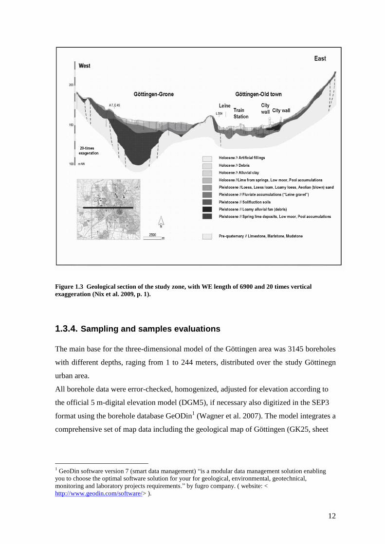
12

Figure 1.3 Geological section of the study zone, with WE length of 6900 and 20 times vertical

exaggeration (Nix et al. 2009, p. 1).

1.3.4. Sampling and samples evaluations

The main base for the three-dimensional model of the Göttingen area was 3145 boreholes

with different depths, raging from 1 to 244 meters, distributed over the study Göttinegn

urban area.

All borehole data were error-checked, homogenized, adjusted for elevation according to

the official 5 m-digital elevation model (DGM5), if necessary also digitized in the SEP3

format using the borehole database GeODin1 (Wagner et al. 2007). The model integrates a

comprehensive set of map data including the geological map of Göttingen (GK25, sheet

1 GeoDin software version 7 (smart data management) “is a modular data management solution enabling

you to choose the optimal software solution for your for geological, environmental, geotechnical,

monitoring and laboratory projects requirements.” by fugro company. ( website: <

http://www.geodin.com/software/> ).

http://www.geodin.com/software/

13

4425), 25 geo-engineering maps from diploma1 mapping projects, as well as geological,

soil type and geomorphological small-scale maps (e.g. Schlie, 1989 and Wunderlich,

1959). In addition more than 30 EW as well as more than 30 NS cross sections was

constructed to use the defined layer boundaries as pre-interpreted support during the 3D

modeling.

Figure 1.4 Exploded view of the central section of the 3D subsoil model (view from southeast, tilted,

extension E/W: 6900 m, extension N/S: 1700 m, vertical exaggeration 15x (Nix et al. 2009, p. 1). For

Description of the model units, see section 1.3.4.

Due to the complex spatial pattern of the Quaternary sediments the information had to be

translated into a reduced set of structures that would preserve the main and relevant

features and guarantee to keep the limited time frame for the modeling within the project.

As a result the following model units were defined:

(1) Anthropogenic fillings,

(2a) floodplain sediments and stream loams of younger Holocene,

(2b) younger Holocene debris flows,

(3) Soft Holocene layers (lime from springs, peat, mud),

(4) Pleistocene loess, loamy loes, and flood loess,

(5a) Pleistocene solifluction soils,

(5b) Pleistocene debris,

(5c) Pleistocene river gravels,

1 German diploma academic system is equivalent to M.Sc. in American academic system.

14

(6) Pleistocene soft layers in subrosion basins,

(7) Pre-quaternary bed rock surface.

Figure 1.4 illustrates the location and distribution of the mentioned layers

(Nix et al. 2009).

In this study, the layer 5 was targeted for modeling, because of its geotechnical

importance and higher complexity. In addition, the anthropogenic fillings and the

superficial sediments were not considered for the geostatistical modeling because they are

rather being homogeneous.

1.3.5. Parameterization

Because of the uneven and sporadic distribution of measured soil physical or mechanical

characteristics, a process was developed to geotechnically describe and estimate the

properties of petrographic layers (Fritz et al. 2007). Basis of the classification was six

major soil classes out of which four observed classes in the study zone of this dissertation

were modeled here (see the summary of classification in Table 1.1 and Table 1.2).

This classification was formed in accordance with the DIN 18196 standard1 based on the

information from petrography, genesis, and soil layer group descriptions in the equidistant

spacing of 0.5 m above this level are assigned to soil classes (Table 1.1 and Table 1.2).

The distribution of soil classes within the three-dimensional sedimentary bodies was

determined using a geostatistical indicator kriging (IK), sequential indicator simulation

(SISIM), and transition-probability Markov chain simulation approaches using the

software WinGslib version 1.5, and TPROGS version 2.1. Here, the probability of the

existence of a soil class is estimated in each cell of the estimation model and the

uncertainty of the estimation was quantified. Then in each estimation point of the model,

the soil class which held the highest probability of occurrence was assigned to the

estimation point. Geostatistical estimation was conducted for the distribution of soil

classes 1-4 in the model units (5a, b, and c).

1 German standard for geotechnical soil classifications based on grain size range, grain size distribution,

plasticity characteristics, organic constituent characteristics, and genesis. For more details refer to Deutsche

Institute Für Normung. "Erd Und Grundbau, Bodenklassifikation Für Bauteschniche Zwecke, DIN 18196."

Erkundung Und Untersuchung Des Baugrunds: Normen. Vol. 13. Berlin [u.a.: Beuth, 1991. 363-66. Print.

15

Table 1.1 Geotechnical unconsolidated sediments classification scheme for sedimants without organic

components (Wagner, 2009).

group geotech-

nical classes petrology main components

(minor components)

facies

A fine-grained sediments

3 clay and silt T, U, (S) clayey-silty limnic sediment

pure clay T, (U, S) clayey limnic sediment

pure silt U, (T, S) silty limnic sediments, loess

B mixed grain-size sediments (clay and/or silt and/or sand)

3 clay, silt and sand

T, U, S clayey to silty floodplain deposits, weathered loess

2, 3 clay and sand T, S, (U) weathered loess

3 silt and sand U, S, (T) loess

2, 3 sand and silt S, U, (T) aeolian sand, sandy loess

C mixed grain-size sediments (clay and/or silt and/or sand, minor gravel)

2 to 3 3

clay, silt and sand, minor gravel

T, U, S, (G) displaced loess and sandy loess, sandy floodplain deposits

3 clay and/ or silt, minor sand and gravel

T, U, (S, G) T-U, (S, G)

displaced loess, marginal fine-grained limnic sediment, crumbled clay

D mixed grain-size sediments (clay and/or silt and/or sand and/or gravel, minor blocks)

2, 3 2 to 3

clay, silt, sand and gravel

T, U, S, G, X solifluction material, weathered hardrock

2, 3 clay, sand and gravel

T, S, G, (U) solifluction material

2 to 3 3

clay, silt and gravel

T, U, G, (S) solifluction material, clayey-silty fan deposit, displaced loess

2, 3 2 to 3

clay and gravel T, G, (U, S) solifluction material

E mixed grain-size sediments (silt and/or sand and/or gravel and/or blocks)

2 to 3 2, 3

clay and gravel, minor blocks

U, G, (X) silty fan deposit, silty fluvial gravel

2 silt, sand, gravel and blocks

U, S, G, X clayey and blocky fan deposit

2, 3 2 to 3

silt, sand and gravel

U, S, G, (T) silty-sandy fan deposit, silty-sandy fluvial gravel

F coarse-grained sediments (sand and/or gravel and/or blocks)

1, 1 to2 sand and gravel S, G, X, (T, U) sandy fluvial gravel, sandy fan deposit

1, (2) pure sand S, (T, U) fluvial sand

1 gravel and blocks G, X, (T, U, S) coarse fluvial gravel

1 pure gravel G, (T, U, S) fluvial gravel

Abbreviations: T: clay; U: silt; S: sand; G: gravel; X: blocks

16

Table 1.2 Geotechnical unconsolidated sediments classification scheme for sedimants with organic

components (Wagner, 2009).

group geote

ch-nical classes

Petrology facies

G organogenetic sediments or sediments with organic constituents

4 slightly organic fine-grained sediments (h1, h2, org, pf or fau)

holocene soil, flood plain deposits, limnic sediment, displaced loess

slightly organic coarse-grained sediments (h1, h2, org, pf or fau)

holocene soil, flood plain deposits

slightly organic mixed grain-size sediments (h1, h2, org, pf or fau)


4 organic fine-grained sediments (h) holocene soil, flood plain deposits, limnic sediment, displaced loess

organic coarse-grained sediments (h)

holocene soil, flood plain deposits

organic mixed grain-size sediments (h)


4 fine-grained sediments with high organic content (h4)

holocene soil, flood plain and swamp deposits

coarse-grained sediments with high organic content (h4)


mixed grain-size sediments with high organic content (h4)


organic clay flood plain and swamp depoits

H freshwater limestone

4 freshwater limestone sinter terraces

Abbreviations: h1: very slightly organic; h2: slightly organic; h or h3: organic; h4: strongly organic

The spatial structures and continuities are usually stronger in the startigraphic directions

such as the layering surfaces.

The classes 5, 6, and 7 refer to the organic sediments, artificial fillings, and hard rock

respectively which have not been explained in Table 1.1 and Table 1.2.

To take the general stratigraphic continuity directions into account and improve the

spatial continuity structure model, a common technique is to model the facies and

reservoir attributes in the modeling grids proportional between the top ad bottom

correlation surfaces (Deutsch 2002, p. 88).

For that reason, the coordinate transformation was applied in this study. More details

about the grids transformation will be discussed in the next sections.

17

1.4. An introduction to the geostatistical modeling methods (a comparison of different methods)

1.4.1. An overview to geostatistics

1.4.1.1. A bit of history:

In the older conception, geostatistics had the meaning of the application of statistics in the

geology or perhaps more generally in the earth sciences. In this sense, statistics was

applied in the earth sciences since long time ago (Myers, 2002). Bertil Matern (born

1917) a forestry scientist and statistician introduced the meaning of the spatial variation

and the importance of the spatial dependence application especially in the forestry

science. In the mid 60th and especially in the mid 70th, the new meaning of the

geostatistics was introduced with relation to the works of Georges Matheron (1930-2000).

Matheron was influenced by Daniel J. Krige, a mining engineer in South Africa, and the

former attempts of the Lev Gandin (1921-1927) a Russian Mathematician in the

Leningrad Hydrogeological Institute. Krige was working on the assessments of the new

gold mines using a limited number of boreholes. Matheron had theorized the important

geostatistical concepts such as the regionalized variables. He was closely applying the

developed methods in mining and petroleum applications. Matheron named the optimal

estimation method of the unknown points using the available observations as “kriging” in

the honor of Krige as a pioneer in geostatistics. Matheron not only explained the basics of

Geostatistics for estimation especially for mining applications but he also paid attention to

the quality of estimations and such concepts as estimation variance (Myers 2002; Myers

2008; Isaaks et al. 1989; and "Danie G. Krige." Wikipedia, Mar. 2012. Web. Apr. 2012).

1.4.1.2. The estimation problem and geostatistics:

A major problem in subsurface modeling is to estimate the attributes in the unknown

points having a limited set of sample data, which can be employed for different cases

such as geotechnical and geological applications. This estimation goal was primarily

addressed by hand-contouring (in two-dimensional slices), providing an insight into the

trends and uncertainty in data (Deutsch 2002, p. 154).

18

Conventional estimation algorithms of the interpolation family, consider several

simplifying assumptions such as constant values considered inside polygons, triangulation

and linear interpolation inside the triangles (representing continuous changes), inverse

distance weighted interpolation methods, etc.

These methods, for example the inverse-distance interpolation, are usually based on the

estimation of the target variables in the unknown positions by means of a linear

combination of neighboring known values. For such estimations, each of the known

values of the surrounding points receives specific weights. For instance in the inverse-

distance method, the weights of the values inside a search radius for the known points

applied for this estimation, are inversely proportional to their distance to the estimation

point:

) z(u d

1 (u)*Z

n

1i

i

i

(1-1)

Where Z*(u) is the estimating function for the location u, z(ui) is one of the neighboring

samples used for estimation, and di is the distance of the data from the estimation point.

To decide which method is the best among the others, some criteria can be defined and

applied such as comparison of the univariate statistics of the estimates and true values,

univariate distribution of errors, and evaluating the bivariate distribution of estimated and

true values. Isaaks and Srivastava (1989) have compared polygonal estimation,

triangulation, local mean, and inverse distance in some case studies (Isaaks et al., 1989)

and represented some features about the efficiencies of these methods such as the

existence of a global bias and smoothing effect (i.e. less variation in estimations in

comparison to those of the true values)in all these methods. These two effects were less

evident in polygonal estimates. The more samples were used in the estimation, the more

smoothing were observed. On the other hand, since the triangulation method showed a

more symmetric errors distribution, the lowest standard deviation, and the lowest inter-

quartile range of the estimations, it was suggested as the best estimation method among

the mentioned techniques to infer a sensible guess for the unknown points (Isaaks et al.

1989, pp. 249-277).

Some attempts were then conducted to perform optimal estimations in some objective

sense. For instance, Daniel Krige was interested in, two criterions of the unbiasedness

(correct overall average) as well as minimizing error variance in the estimations

(Khojasteh 2002). For this purpose, kriging as an estimation method was developed by

Georges Matheron (1961/62) which uses a linear combination of the known neighboring

19

samples consistent with the two mentioned criteria. The kriging is usually abbreviated as

the BLUE (the Best Linear Unbiased Estimator).

A regionalized variable is a variable (such as litofacies, porosity, or permeability) that

may take different values at different spatial locations (Deutsch 2002, p. 345).

The two different terms of estimation and simulation have been often addressed in this

context.

An estimation technique like kriging makes a single best guess of the unknown using the

assumed spatial relationship between the data and the unknown and is locally accurate

since it minimizes the local errors independent of what the global map of estimates may

look like. The estimated maps usually represent much smoother outputs (Caers 2000, pp.

815-816).

The geostatistical simulation methods on the other hand, offer mapping methods which

create non-unique and non-smooth results (Caers 2000, pp. 815-816). These methods are

globally accurate rather than locally accurate. The conditional geostatistical simulation

methods generate a set of possible equi-probable realizations which are conditioned to the

available observations while having very close global statistical behaviors (e.g.

variograms) to those of the reality. Having multiple simulated realizations, one is also

able to evaluate the global uncertainties and risks.

1.4.2. Some basic concepts in geostatistics

There are some basic terms and concepts in geostatistics which should be introduced prior

to any geostatistical discussion. Some of them such as; random function, random variable,

discrete and continuous random variables, regionalized variable, and stationarity

assumptions were described very briefly here:

(a) Random function (RF):

Geostatistics is basically founded on the concept of Random Functions (RF), by which

the set of unknown attribute values z(u) at each location of u, is regarded as a set of

spatially dependent random variables (RV) (Goovaerts 1997, p. 63) . With the concept of

20

the random function, one can recognize and model structures in the spatial variation of the

attribute (Goovaerts 1997, p. 63).

A group of spatially distributed samples can be considered as a realization of a random

function (Matheron 1963).

(b) Random variable (RV):

According to Goovaerts (1997, p. 63), a random variable can be defined as following:

“A variable, that can take a series of outcome values according to some probability

distribution”.

A random variable can be either a discrete or a continuous random variable.

(c) Regionalized variable (ReV):

A variable distributed in space (or time) that can take different values in different spatial

locations is termed as a regionalized variable (Deutsch 2002, p. 345). Geologic facies

types or geotechnical soil types in different points are examples of categorical

regionalized variables.

According to the regionalized variable theory (RVT), a set of regionalized variables

includes three different relationships; structural part or trend, correlated variation, and

uncorrelated variation or noise. In the geostatistics the main focus is on modeling the

correlated variation element of the regionalized variable (Hattermann 2011).

21

Figure 1.5 The stationarity of means for a regionalized variable, (A): referring to a stationary mean,

(B): to a non-stationary mean with a trend, and (C): non-stationary case (Hattermann 2011, p. 17).

(d) Stationarity assumptions:

Stationarity is one of the most essential assumptions and decisions that should be

considered for a random function in the geostatistical techniques. Stationarity implies that

the statistics (such as mean, variance, covariance, and so on) is independent of the

location of its calculation in the study area. For instance, a variogram can often be

assumed stationary because it can be applied over the entire area which has been

computed. The variogram in the circumstance of the stationarity, can be regarded a

function of the separation vector (lag) between the pairs of points and independent of the

location. It is the measure of spatial variability for separation vectors (Deutsch 2002, p.

346).

The stationarity is defined in terms of the first- and second-order moments of the samples

random function, and stationarity degrees related to the special moments that stay

unchanged in the study area (Hohn 1991, p. 23)

The expectation of the distribution function of a random variable )(uZ at location u is:

)()}({ umuZE (1-2)

This expectation which is a first-order moment of the )(uZ distribution can be dependent

on u.

22

The four essential degrees of stationarity in geostatistics are; strict stationarity, second-

order stationarity, the intrinsic hypothesis, and quasi-stationarity. To define the

stationarity assumptions easier, the concept of the spatial law of a random function can be

introduced here. The spatial law of a random function can be termed as all observed

distribution functions in all prospective locations of the study area. The referred

stationarity assumptions have been explained briefly here as following:

1. Strict stationarity:

The spatial law between any pair of random variables { )( 1uZ , )( 2uZ … )( muZ } and

{ )( 1 huZ , )( 2 huZ … )( huZ m } is invariant in the strict stationarity condition. In

other words, the distribution function (of a random function) does not change in terms

of the separation vector of h.

The strict stationarity assumption is not necessary in most of the geostatistical

purposes since these applications often need only the first two moments (Hohn 1991,

pp. 24-25).

2. Second-order stationarity:

The second-order stationarity requires:

(a) Invariant expectation:

fixumuZE )()}({ (1-3)

(b) The covariance dependent only on the separation vector:

2)()()( mhuZuZShC for each u (1-4)

The stationarity of covariance C(h) is equal to the stationarity of the variance

and semivariogram:

)()()()0(2

uZVarumuZEC (1-5)

)()0(2/})()({)( hCCuZhuZEhg (1-6)

Under the second-order stationarity conditions, the semivariogram or covariance can

be chosen to measure the spatial auto- or cross-correlations (Hohn 1991, pp. 24-25).

3. The intrinsic hypothesis:

In the intrinsic hypothesis conditions, the expected first-moment and semivariogram

values are invariant. Therefore, the intrinsic hypothesis is a reduced form of the

second-order stationarity since it does not require the stationarity of the covariance

23

but just the existence of a finite variance C(0). For most of the geostatistical

applications, the intrinsic hypothesis is sufficient.

If the random variables and their functions do not conform to the conditions

described above and therefore represent a kind of dependence of the functions on the

location, they bear a kind of characteristics called ‘trend’ (Hohn 1991, pp. 24-25).

4. Quasi-stationarity:

The studied variables may in reality have a trend (or show a ‘drift’) over the study

area. Although such a variable is not stationary in the insight of definitions mentioned

above, a sort of local stationarity can be accepted in practice. This means that when

the maximum applied distance in semivariogram or covariance calculation is much

smaller relative to the trend range, the quasi-stationarity circumstance can be accepted

(Hohn 1991, pp. 24-25).

(e) Detecting the existence of a trend:

Obviously, to identify the existence of a trend in regionalized variables, the most

straightforward approach could be to plot the target variable against the distance in

different directions and evaluate its general changes. To make a general trend clearer, the

moving average or similar method can also be applied. In the case of the existence of a

trend, a systematic change should be distinguished in the general variation of the values

along the distance axes (similar to time-series analyses, e.g. Fahmy and Elsayed 2006;

Smith 1989). As an example, suppose that there is a coal layer with variations in its

thickness and the aim is to model and estimate the thickness of this layer. Generally,

three types of variations in the thickness of the example layer could be identified; erratic,

periodic, and systematic. Assume that, in general, the mentioned layer is getting thicker

and thicker in a specific direction, let say from west to the east. However, in the local

scale, the layer thickness shows some erratic changes while these changes have an

algebraic sum of zero. The first part of the variations (i.e. the general systematic changes),

are the trends of the investigated parameter. Therefore, plotting the thickness of the

mentioned layer against the distance will represent how the thickness is increasing in the

East-West direction in general, which can be modeled using a regression model.

Subsequently, the thickness of the layer will be equal to the amount of the mentioned

trend plus a local erratic variation:

24

eumuZ )()( * (1-7)

where Z(u) stands for the amount of the required attribute (like thickness) in the location

u, m*(u) is the estimated local average of that attribute, and e is the erratic term of the

variation of the cited attribute or the error representing the difference between the

estimation of general trend and the real values.

In the geostatistical methods like kriging, the local erratic variation term of the

regionalized variable (i.e. e equation (1-7)) can also be modeled.

All geological processes convey a sort of trend in distribution of petrophysical

properties, such as fining or coarsening upward. Hence, the large-scale negative

correlations indicative of a geologic trend is appeared as the variogram increase over the

sill variance of C(0)= 2 (Deutsch 2002, p. 117). From the above discussion, an

important practical conclusion can be inferred that one of the best and most practical

indicatives of the existence of a trend within the study zone is to plot the sample

variogram and the theoretical sill, and evaluate the general behavior of the variogram plot

relative to the theoretical sill. If the sample variogram increasingly exceeds the expected

(theoretical) sill, the prevalence of a trend can be concluded. The expected sill can be

considered as the variance of a data-set, i.e. C(0)= 2 , for the continuous variables, and

p(1-p) for categorical variables where 2 is the continuous data variance and p is the

proportion of a category in the categorical data. Another concept related to the trend is the

areal trend that may cause a zonal anisotropy between the horizontal and vertical

variograms. The concept of the zonal anisotropy has been discussed in the next sections.

The areal trend can cause the vertical variograms to be unable to meet the full variability

of the attributes. Therefore, the vertical variogram stay below the theoretical sill of the

variogram.

25

Figure 1.6 An example of the case of the presence of areal trends has been depicted here. In such

cases, each well does not capture the full range of variability. In this example, well A faces mostly

high values while the low values are observed in well B (from Gringarten and Deutsch 2001, p. 514).

Figure 1.7 Vertical semivariogram with a zonal anisotropy in which the variogram does not reach its

expected sill (Deutsch 2002, p. 121).

Figure 1.6 illiterates the effect of areal variability on the coverage of the variability of the

attributes in the vertical direction (Deutsch 2002, pp. 121-122).

As discussed before, the first crucial stage in all geostatistical modeling procedures is to

set the right model variables, to ensure, with an acceptable tolerance, that these

characteristics can be modeled as a stationary variable along the study zone. In the case of

the presence of a significant trend, the trend should be modeled and removed prior to any

geostatistical modeling step. Finally, the trend can be added back to the estimations or

26

simulation values over again. The action of removing the existing trends is called

detrending. If a negligible trend is detected, the stationarity can be accepted and the

regular geostatistical procedures can be followed (Deutsch 2002, p. 122).

The above discussions are more applicable to the continuous variables. Nevertheless, the

same principles can be applied to the categorical variables modeling. As it will be

explained in the next sections, the indicator geostatistical methods are usually applied in

modeling the categorical variables. For such indicator geostatistical analyses, to check

whether or not any trend exists, the proportions of the categories (e.g. facies or soil types)

are considered instead of the variable means of the continuous variables. In other words,

the proportions or existence probabilities of the categories are evaluated, their variations

are modeled, and the unknown probabilities are estimated (or simulated). The trends in

facies proportions usually exists and is likely in either areal or vertical directions and the

trend models construction follows the same approach as for that of the continuous

variables (Deutsch 2002, p. 186-187). Then the significant trends in proportions can be

removed prior to the indicator geostatistical analyses. To have a rough evaluation of the

probable existing trends in different parameters during this study, three approaches have

been applied:

(a) Drawing the scatter-plots of each parameter against the distance.

(b) Plotting the location map of the boreholes which include the investigated

parameters.

(c) Inspect the behavior of the indicator variograms for each soil category.

To achieve the best stationarity conditions, the zones and layers have been separated into

the a few more similar and homogeneous sub-zones. For example, the deep holes were

put aside and the slope sides of the basin were also considered separately.

(f) Variograms and models:

Modeling the regionalization is more beyond a simple smooth interpolation among the

points. In order to do geostatistical modeling, it is necessary to explore the spatial

variability in the existing data-set (Gringarten 2001).

27

Figure 1.8 A typical variogram that can be applied in spatial visibilities modeling. The dots show the

sample variogram and the solid curve represents the model variogram. The straight thin solid lines

project the important variogram parameters of range (a) and sill (c).

Recalling the concept of the regionalized variable, the correlated stochastic component

can be modeled in the next estimation or simulation stages. Obviously, any existing trends

can be modeled and removed beforehand. Modeling the spatial variability structure of a

regionalized variable can be conducted using various measures and methods such as two-

point statistics; including the covariograms or correlograms to measure the similarities,

variograms or madograms as the measures of dissimilarities, and the multiple-point

statistical methods that go beyond the two-point statistics in spatial variability modeling.

These concepts have been elaborated in different sources and will not be addressed here

except very briefly for variogram and its analytical models. A variogram which represents

the degree of spatial dissimilarities for a regionalized variable can be expressed in

mathematical terms as a mean variance of the pairs of the values separated with the

separation vector of h, plotted for different separation vectors (Gringarten 2001).

Similarly, this spatial correlation can be expressed among more than one variable using

spatial cross-covariance functions (covariance of the variables with other variables) which

are called covariograms. A typical variogram increases with the increase of the separation

vector to a certain distance called range where the variogram will reach to a plateau

called sill. The sill expectedly should be, in its full distance, nearly equal to the data

28

variance for the continuous variable (i.e. 2)0()0( C ) and p(1-p) for the indicator

variograms. In this expression, p represents the proportion of the corresponding category.

A sample variogram of a regionalized variable therefore, can be defined as following:

2)(

1

* )()()(2

1)(

hN

hxZxZhN

h (1-8)

where N(h) is the pairs number of the data locations which are separated by the vector h

(Isaaks 1989, p. 82). It should be considered that in most of the scientific sources, the

term of “semivariogram” was applied for the above definition. However, for

simplification reasons (as it has been used also in some other literature), it will usually be

referred as “variogram” in this context.

Equally, if the indicator values (I), are replaced with regionalized variables of Z in the

definition of the variogram, the sample indicator variogram will be expressed as

following:

2)(

1

*)()(

)(2

1)(

hN

I hxIxIhN

h (1-9)

Such an indicator variogram is a valuable tool for modeling the spatial variability of

indicator values in modeling categorical variables and estimating the local probability

distribution functions. The act of fitting analytical models to the variograms is termed

variography.

The above formulas provide a set of experimental values that reflect the spatial

variability structure but neither in all distances nor in all directions. Hence, analytical

models should be fitted to the experimental (or sample) variograms to; deduce the

variogram values in all points, smooth out the effects of fluctuations, and ensure the

positive definiteness property of variograms (Goovaerts 1997, p. 87; Deutsch 2002).

Positive-definiteness is an indispensable perquisite for solving the estimation equations of

kriging to ensure that the kriging variance is positive and the estimation equations are

solvable. Using specific standard mathematical variogram models to be fitted to the

experimental variograms can ensure the positive-definiteness characteristic of the

estimation models (Goovaerts 1997, p. 87; Deutsch 2002, p. 131).

29

Pure nugget effect, spherical, exponential, Gaussian, and power models are the most

frequently used basic variogram models. The mathematical definitions of the most

important basic theoretical isotropic variogram models have been brought in different

geostatistical resources. Yet, as an instance and one of the most important permissible

mathematical variogram models, the equation for standardized isotropic spherical model

has been brought here:

Spherical model with a range of a:

otherwise

ahifa

h

a

h

a

hSphhg

1

.5.0.5.1)(

3

(1-10)

To model the spatial variability of a regionalized variable, a composition of the

mentioned models may offer a better fit. The first four models are bounded because they

reach actually or practically to their sill (which was 1 in the above formula as their

standardized sill). The real sill values can be considered in the models by multiplication

of the sill values by the standardized models (Goovaerts 1997, p. 88).

The variograms may show different behaviors in different directions. This characteristic

is recognized with the phenomenon of anisotropy (Sarma 2009; Goovaerts 1997). On the

other hand, the structure of the data variations (e.g. variograms), does not change in

different directions in an isotropic model. The variogram anisotropy can be of two major

types; the geometric (also called elliptic), and zonal (also called stratified). In the

geometric anisotropy, the variogram sills remain unchanged whereas their range changes

in various directions. This sort of anisotropy can be illustrated with an anisotropy ellipse

or ellipsoid and expressed by anisotropy ratio, for instance, in the case of two-

dimensional studies:

)/( 21 aab (1-11)

in which the a1 stands for the variogram range in one principal anisotropic direction and

a2 is the variogram range in another principal anisotropic direction for a bounded

variogram or:

)/( 21 slopeslopeb (1-12)

for an unbounded variogram (Sarma 2009).

30

With the anisotropy ratio, by a simple transformation, all the geostatistical equations can

be reformulated based on the equations of the isotropic case.

Figure 1.9 illustrates the case of the geometric anisotropy in two variograms.

Figure 1.9 Anisotropic variograms; (A) variogram with the same sill and (B) linear variogram with

different slopes (Sarma 2009, p. 83).

Figure 1.10 Samples of elliptical anisotropy; (A) main axes follow the direction of the co-ordinate

axes and (B) main axes do not follow the direction of the co-ordinate axes (Sarma, 2009 p. 84).

In the case of zonal anisotropy, the sills are not equal in different directions, and in

general, the variograms in various directions represent a complex behavior. Usually, in

such cases, the variogram is split into two components; an isotropic variogram plus a

variogram depending only on the vertical direction (Hohn 1999).

In this study, the zonal anisotropy between the horizontal and vertical variograms was

obvious in indicator variograms. However, the problem was seen that the vertical

indicator variograms could not meet all the variability because of the much shorter

investigation distance. The component of the vertical indicator variograms played the role

of the nugget effect for the horizontal indicator variograms. Therefore, the three-

dimensional variograms were the sum of the two mentioned components.

31

1.4.3. Kriging and geostatistical simulation basics

Let’s start with an example to address the importance and advantage of using the kriging

estimator in practical problems, especially in the case of subsurface studies where the

access and information are more limited.

Figure 1.11 An illustration of the subsurface estimation problem in environmental applications. W1

to W5 represent the drilling locations for getting subsurface samples or measurements.

Suppose that in an environmental survey, the monitoring of the extent and immigration of

contaminants and proper remediation planning is aimed. Yet, due to the technical and

economical limitations, it is almost impossible to have a full measurement of the required

parameters and characteristics throughout the subsurface. In this example, assume that, all

the available and reliable information and data could be achieved through a limited

number of samples taken from some boreholes (W1 to W5).

Therefore, the required characteristics are known in a few points but they are unknown

elsewhere which is the majority of the investigation zone and the prediction of the facies

types within which the mentioned characteristics are targeted would be the first step in

modeling.

As it has already been discussed, there are different approaches to estimate the required

characteristics in the unknown points which fall in two main categories of structure

imitating and process-imitating. In the structure-imitating methods, the observed patterns

and structures are modeled without directly considering the processes responsible of their

creations. The process-imitating techniques are not the issue of this study (Falivene et al.

2007, p. 200; Koltermann and Gorelick 1996).

The kriging aim is to achieve the “Best Linear Unbiased Estimation” (B.L.U.E.) by

assigning weights to surrounding samples to an estimation point (Clark 1979, p. 100). In

32

comparison to the conventional estimation techniques, kriging takes also the spatial

variability structure, the samples distribution patterns, and the probable anisotropies into

account.

Although kriging is basically developed with the linear underlying presumptions, the

non-linear estimation frameworks can also be defined in the kriging approach. These non-

linear estimations are termed non-linear kriging which fit better to the most practical

applications since most data sets do not obey the multivariate Gaussian assumptions

(Hohn 1999, pp. 134-135).

Kriging estimator contains two essential properties (Armstrong 1998, p. 92; Deutsch

2002, p. 154):

(a) Unbiasedness, which means that the average of the estimation errors (the difference

of real and estimated values) are zero :

v vE[z z ] 0 (1-13)

in which *z is estimated and z is the true value.

(b) Minimum estimation error, which means that the average squared difference between

the true and estimated values (square error) should be minimum:

2 2

E v vE[(z z ) ]minimum (1-14)

These equations obey stationarity assumptions.

Based on the type of the mean of a regionalized variable in kriging equations, kriging is

categorized into different types such as; simple kriging (SK) in which the mean is

constant and known, ordinary kriging (OK) in which the mean is constant but unknown,

and universal kriging (UK) where the mean is unknown and inconstant.

When a stationarity or quasi-stationarity conditions is met, using the OK (ordinary

kriging) or SK (simple kriging) would be suitable. However, in the case of significant

trends, detrending should be performed first. In this case, using the ordinary or simple

kriging was identified to be adequate due to the stationarity or quasi-stationarity

conditions in the existing data-set of the soil types.

The final equations of the kriging with the ordinary kriging conditions (i.e. constant and

unknown mean of the variable) only are brought here.

33

Rewriting the kriging equations for ordinary kriging, the estimation equation can be

summarized as:

i

n

v i vi 1

z Z (1-15)

where *

vz is the estimate value based on the linear combination of ivZ known

neighboring values and i are kriging weights and n is the number of neighboring points.

The result of equation (1-15) will be:

n

ii 1

1 (1-16)

and a set of equations for ordinary kriging can be written as:

n

j i j ij 1

n

jj 1

C(v , v ) C(v , v) i 1,2,..., n

1

(1-17)

i jC(V ,V ) in the above equations, is the average covariance between pairs of points and

can be calculated using auxiliary functions. Therefore, having covariance or variogram

functions (i.e. variogram models), a set of n+1 equation exist with n+1 unknown

parameters including n, i kriging weights and a Lagrange parameter.

In the indicator geostatistical approaches, a value so-called indicator is assigned to each

sample point so that the indicator is set to one (1) when the category exists at that point

and zero (0) otherwise, i.e. :

kuclif

kuclif

uI k

)(0

)(1

)( k=1, 2, … n (1-17)

where )(ucl is the true class that exists in the location u , k is a category of soils between

1 and n , and n is the number of existing categories.

The same variography and estimation methods are used for the indicators to achieve the

estimations and simulation. The outcome of the indicator kriging, therefore, is the

probabilities of the occurrence of each class at each location. In this study, the assigned

category to each estimation point from the indicator kriging was the soil class that held

the highest probability of occurrence estimated from indicator kriging.

34

Although, the indicator kriging method is suitable in estimation of the probability of the

occurrence of the facies, it faces some critical problems in modeling and estimating such

as; the estimated values out of (0,1) range (nonsense probabilities) and vague

experimental variograms (because of insufficient data ) that are difficult and uncertain to

model.

As referred before, kriging includes a problem so called smoothing effect. As a result,

the global statistics of the estimations (including the univariate statistics, e.g. mean and

histogram, and bivariate statistics e.g. variogram and covariogram) are different from

those of the real statistics. In some practical problems such as flow simulating inside a

hydrocarbon reservoir or detecting points with high vulnerability to contamination, the

smoothing effect becomes a major drawback for kriging methods since the subtle

variations are very important in such cases (Yamamoto, 2005).

Geostatistical simulation is an alternative to overcome the smoothing effect problem by

producing a set of equi-probable results which resemble the reality in terms of the global

behaviors and reproducing the fine variations. This set of realizations can be evaluated

later as different possible scenarios for the reality (Caers 2005, p. 13).

Geostatistical simulation methods can be categorized into two broad groups of sequential

and non-sequential as well as two main groups of conditional and unconditional methods.

In the sequential simulation methods, the simulation is started from a simulation grid

node and goes forward. Each time, the input data and the previously simulated values are

considered for the simulation of the next grid node. The sequential indicator simulation

method is an example of sequential simulation methods in geostatistics. In the non-

sequential methods on the other hand, the simulation is performed all at once, such as the

LU decomposition and p-filed simulation methods (Caers 2005).

In conditional simulation, the local conditional cumulative density function (CCDF) is

approximated in each simulation node of the simulation grid and a random variable is

drawn out of it, then using the existing data and already simulated points, the simulation

is followed in a random path which visits all the simulation nodes. More details about the

conditional geostatistical simulation are brought in relevant literature.

Sequential Gaussian (SGSIM) and Sequential indicator simulation (SISIM) methods are

among conditional geostatistical simulation methods which are broadly used in various

applications. However, SGS and SIS have some shortcomings. In SGSIM, the Gaussian

assumption is not always reliable or readily verifiable. On the other hand, SISIM faces the

35

same difficulties as indicator kriging in modeling and statistics faces; i.e. tedious and

from time to time vague variogram models, order-relation violations and sometimes

nonrealistic probabilities inferred from indicator kriging. For example, the estimated

probability may become greater than one or less than zero. Another problem of the SISIM

method is the difficulty of considering the inter-class relations among the categories.

Considering the inter-class correlation can certainly improve the estimation quality

especially for in the case of limited number of samples. Although one also may employ

the methods like cokriging that take the inter-class correlations into account. However,

cokriging method requires some constraints and special conditions in building the

covariogram models that make its application more complicated.

Some geostatistical simulation methods based on Markov chains, which have been

applied in the coming sections, have paved the way to improve the modeling of variability

and to overcome the problems included in the traditional geostatistical methods.

In general, according to the author’s opinion and knowledge, some remarkable problems

in the traditional geostatistical methods should be taken into consideration, such as

variogram modeling in the lack of sufficient data, insufficiency of two-point statistics in

capturing complexities, severely mathematical view in traditional methods, linearity of

estimators, and etc.

In the coming section, some geostatistical methods have been compared together based on

the literature review.

1.4.4. A comparison of some geostatistical modeling (estimation/simulation) methods, considering their applications:

During the literature review according to the advisors’ recommendations, plenty of

different papers and books were reviewed aiming at finding the strength and weaknesses

of different geostatistical modeling methods and selecting their best in terms of the

applicability of the method in such cases, availability of the software, and the efficiency

of the method.

Among a big variety of reviewed geostatistical modeling and simulation techniques, only

the most important of them have been pointed out here.

36

Table 1.3 summarizes the basics, applications, advantages, disadvantages, and software

of some geostatistical methods which were reviewed in the initial stage of this research to

compare and choose the most suitable of them for applying in this study.

The reviewed methods can be put into the following groups:

(1) Markov-chain based methods: for example: transition probability-based Markov

chain (TP/MC), coupled Markov chain (CMC), triple Markov chains (TPC),

Markov chain geostatistics (MCG), hierarchical architecture modeling of

continuous characteristics using Markov chains (Ritzi 2007).

(2) Multiple-point statistics (MPS).

(3) Bayesian maximum entropy (BME).

Because, bringing the complete summary of all the corresponding discussions here would

be too tedious and lengthy to and to make it easier and quicker to compare and access all

of the reviewed methods together with their most important features, the required

information about them have been summarized in Table 1.3.

1.4.5. Summary and highlights of the compared methods

The most important points about the mentioned comparison of the various geostatistical

modeling methods can be summarized as following:

(a) Modeling the boundaries of categories prior to modeling their containing

continuous variables would lead to significant improvements in the resulting

models.

(b) Most of the mentioned Markov chains-based models facilitate the integration of

subjective and interpretive information (such as geology and expert’s

interpretations) into the models and result in considerable improvement in

modeling spatial continuity.

(c) Stochastic simulations based on Markov chains can lessen some shortcomings of

conventional geostatistical methods theoretically because of:

o Being non-linear.

o Being neither completely stochastic nor completely deterministic (intermediate

stochastic).

37

o Facilitating consideration of the inter-class correlations.

o Reducing the order-relation problem of IK1.

(d) Two-point statistics such as variograms can not completely capture the spatial

variability complications, especially when heterogeneity has a rather complex

geometry. MPS1 is a solution to overcome this problem.

(e) Considering a general primary knowledge and updating the posterior distribution

function like in BME1 method seem very effective ways of improving stochastic

modeling.

(f) Traditional geostatistical approaches such as IK, suffer from several problems

such as order-relation violations and the weakness in complex subsurface

heterogeneities reconstruction specially about modeling spatial connectivity

among them and particularly when samples are sparse (Bierkens and Weerts 1994,

p. 283; Li and Zhang 2008, p. 158).This might be due to difficulty in making

inter-class correlations and being linear (Li and Zhang 2008, p. 158).

(g) Although the proposed methods based on the direct use of Markov chains (MCs)

have significant advantages over other methods especially over traditional

geostatistical methods, they still may have some shortcomings such as these:

o Because they are among unilateral processes, they may generate inclined

patterns (i.e. diagonal trends) due to the asymmetric neighborhoods used in

multidimensional simulations. To reduce or avoid this problem, symmetric or

quasi-symmetric path may be defined (Davis 2002, p. 575). However, the

transition-probability Markov chain (TP/MC) approach applied in the present

study does not implement asymmetric paths and expectedly should not

produce such problems.

o Pattern inclinations and artifacts are possible to occur. This is especially about

CMC2 method when asymmetric or quasi-asymmetric paths are not used. They

may also occur in MCG. In addition, using an asymmetric or quasi-

asymmetric path may reduce the positive feature of considering asymmetry as

an advantage of these methods (Park et al. 2007, p. 910).

o In TPC2 and MCG

2 methods, the main formulation is suited for two-

dimensional problems. The direct and easy formulations of these methods for

1 IK stands for indicator kriging, MPS multiple-point statistics, and BME for Bayesian maximum entropy.

2 CMC stands for coupled Markov chain, TPC for triple Markov chains, MCG for Markov chain

geostatistics, and TPs for transition-probabilities.

38

three-dimensional problems and with considering three-dimensional modeling

scheme are hardly mentioned except for CMC that suffers other problems.

o In CMC, underestimation of small classes and overestimation of big classes

especially when samples are few and sparse may cause unrealistic patterns.

o Some other problems in CMC, TPC and MCG include; difficulties with

accounting for anisotropies and large-scale features (e.g. in MCG because of

the use of small, systematic neighborhood system), practical problems with

calculating TPs particularly from sparse data, the problem of inferring multi-

step TPs form one-step TPs and some theoretical simplification problems such

as conditional independence assumptions (Li and Chuanrong 2008, pp. 159-

163).

(h) BME and MPS seem to be too dependent on external information sources

rather than available data-set, such as training images, interpretations, and so

on.

(i) Most of the mentioned methods have been applied in specific practical

problems while they can be applied in the other fields as well. It seems that

the main difference is due to abundance and the sort of available data in

different applications, e.g. in mining problems, various and abundant data

usually exists whereas there is little data in environmental problems.

However, in special cases, the problems may become more similar. For

instance, in the primary exploration stages of hydrocarbon reservoirs, little

information may exist.

Some other geostatistical methods such as truncated Gaussian and truncated

plurigaussian methods as well as cleaning cell-based methods for modeling the soil

lithofacies can also be applied for modeling the geotechnical soil classes. The first two

methods are based on generating the realizations of one or more Gaussian continuous

random variable and truncating them in specific thresholds to achieve the required

categorical variables. More details and their comparison with the techniques applied in

this study have been brought in Chapter 7.

In general, due to the practical and theoretical situation of this project, the best proposed method

among the mentioned methods according to the literature should be TP/MC method.

39

Table 1.3 Practical summary and comparison of some geostatistical methods based on main framework and the reasons of using them.

Method group The reason for using this

method group

Method

subgroup

Why this method, where, and

the philosophy of its

application?

Main basics and assumptions

of the method

Main framework of the

method

Markov Chains

(MC)

1. Intermediate between

completely stochastic and

deterministic processes, i.e. the

processes is expected to be only

partially stochastic.1

2. Non-linear.

3. Probable dependency

between variables in time and

space and the Walter’s law of

facies succession about

geological or similar sequences.

4. Easier integration of

geological data into models.2

5. Easier cross-correlations.3

Transition probability-based

indicator geostatistics (TP/MC)

1. Improving spatial continuity

modeling, taking some geological

information into account.

2. To overcome vague indicator

variography.

3. Avoid some IK problems like order

relation violations.

4. Incorporating geological/physical

information in modeling.

5. Suitable for categorical data.

6. Asymmetry can be considered.

1. Existence of Markov property.

2. All IK equation can be rewritten in

terms of transition probabilities.4.

3. Using conceptual information like

mean length or proportion of a facies

can help us to make better spatial

continuity models.

1. Get, estimate or calculate the mean

length and proportion of each different

lithofacies.

2. Calculate the 3D transition

probabilities in different distances and

between each 2 categories.

3. The model parameters of transition

probabilities or (co)variograms can be

modeled using the proportions and the

mean lengths of each category.5

5. Perform IK using TP equations.

6. Perform SISIM using TP equations.

Simulated annealing also can be

used to improve the simulations.6

Coupled Markov chain (CMC)

1. Straight-forward modeling and

easier conditioning to available data.

2. Taking geological information into

account.

1. Existence of Markov property.

2. Conditional independence of

samples.7

3. Two single MCs (in 2D or 3 single

chains are forced to move to equal

states.7

1. Calculating the Markovian vertical

TPs using borehole data and inferring

the horizontal TPs using Walther’s law

(transiograms and modeling them).

2. Making grids and Inserting well data

in their location as conditioning data.

3. Calculating the probability of

occurring each states, using the relevant

equation; (e.g. for 2D problem with

Equation. (1-26)) row-wise and from

top to bottom and determining the

succeeding state (which would be

drawn from the CDF of all states at that

point, randomly).

4. Filling out the remaining cells one by

one with similar procedure.8

Triplex Markov chain

geostatistics (TMC)

1. In soil problems with no sparse

samples and soil line measurements.

2. Avoiding trends in produced patterns

despite CMC method.

1. The same assumptions of CMC

2. The simulation path is modified to

avoid directional effects and trended

patterns.

3. Divide area to windows inside

survey lines and walk in two opposite

directions.

4. Uses 2 CMSs from 3 independent 1-

D MCs.3

1. Is according to the same basics of

CMC.

2. Two CMCs from three independent

CMCs are used, i.e. from right to

left, from left to right and from top

to bottom.

3. Applying the simulation inside

windows that are partitioned inside

survey lines, row-wise in opposite

directions.

Markov chain geostatistics

(MCG)

1. Direct application of MC in

simulation (esp. soil problems)

2. To overcome small-class

underestimation problem of CMC.

1. Only one single MC exists in space

which has its CPD in each location

entirely dependent on its nearest

known neighbours in different

directions.9

2. The conditional independence is

theoretically correct in Pickard (1980)

1. Applies a similar framework as the

CMC but it uses only the nearest

known points of estimation points

and a single MC rather than coupling

MCs.10

2. Transition probabilities among each

pairs of classes are calculated, based

40

random field for sparse samples, when

the nearest known neighbours in

cardinal directions are considered.9

on the distances and modeled.

3. The CPD (conditional probability

distribution) is calculated using the

equation (**).

4. Drawing a random class, based on

the above CPD and continuing the

procedure.

Hierarchical architecture

modelling (by: R. Ritzi)

1. Incorporating analogue data

(outcrops…)

2. Improving semivariogram

modelling of continuous variables (e.g.

permeability) and its estimation by

univariate statistics, transition

probabilities and proportions.

3. When Sediments show hierarchical

structure.

4. As usually more categorical data than

continuous is available.

1. Sediments usually represent

hierarchical structure.

2. The permeability variogram is a

linear summation of the auto

variograms and cross variograms for

defined unit types, weighted by

proportions and transition probabilities

of unit types.11

3. The sample variogram can be

approximated using only cross-

transition probabilities and the

univariate statistics (mean and variance)

for permeability within unit types.12

1. Determine and classify the different

levels of hierarchies of sedimentary

facies.

2. Calculate the auto- and cross-

transitions and proportions of each

category.

3. Calculating the univariate statistics

(variance and mean) of continuous

parameter (e.g. permeability) in

different hierarchical levels.

4. Having the calculated parameters,

one can approximate the variogram

model for continuous variable.

Multiple-point statistics

(MPS)

Two-point statistics such as

variograms can not capture the

complex heterogeneities

MPS ( continuous)

1. Bivariate statistic (e.g. variograms)

can not capture complex

heterogeneities (e.g. meanders,

channel (sand) bodies…).

2. Solve the problems of object-based

methods e.g. too much time-consuming,

limitations when sampling is dense

relative to average object size.13

1. Analogue data can help us to make

complicated heterogeneity models.

2. Proper training images can help us to

fill information gaps.

Stationarity and ergodicity assumptions

should be considered (for training

images, etc.).

1. Finding the most general prior

distribution (no specific).

2. Considering specific knowledge,

including hard and soft data.

3. Information from stages 1 and 2 is

processed by means of logical data.14

MPS (categorical)

Bayesian maximum entropy

(BME)

Easier integration of different

sources of information and

physical or expert’s knowledge

or interpretation.

Suitable for little data

condition.

BME (continuous)

1. Offers a nonlinear model.

2. Taking different sources of

information (hard and soft) into

account.15

1. Available hard & soft data and

expert’s knowledge can be applied.

2. Maximizing the entropy maximizes

the information.

3. Posterior probabilities can be

analyzed to get favourite

assessments.

3. Finding the most general prior

distribution (no specific).

4. Considering specific knowledge,

including hard and soft data.

3. Information from stages 1 and 2 is

processed by means of logical data.14

BME (categorical)

41

Table 1.4 Practical summary and comparison of some geostatistical methods based on the advantages of their applications pros and cons, researchers, where they have been applied and software.

Method group Method

subgroup

Advantages (pros) of

using this method

Disadvantages

(cons) of using this

method

Requirements of this

method

Pioneer

researchers

The fields where

the method has

been applied in

real cases

Proposed

applications Software

Markov Chains

(MC)

Transition

probability-Markov

chain indicator

geostatistics

(TP/MC)

1. Making it easier to

integrate indirect, subjective,

or conceptual information.

2. Improving the

understanding of spatial

continuality measures and

facilitating the modeling of

geologically acceptable

spatial continuity measures

(e.g. variograms).

3. Facilitating the full use of

inter-class correlations.16

4. Reducing the order-

relation problem of IK.17

1. Due to the similar

framework to

traditional IK, order-

relation violations

may still be

encountered.

2. Long simulation time

and sometimes

demanding model

fitting procedure.

1. Having

information/interpretations

about the mean length,

juxtapositioning patterns

and proportion of facies.

2. Verification of having

Markov property.

3. Possibility of

calculating, estimating and

making 3D transition

probability models.

Steven F. Carle,

Graham E. Fogg,

Weissmann, Gary

Hydrogeology and

hydrology18

,

environmental

problems19

,

sedimentary structures

analysis19

, transports

in porous materials19

,

solute and tracer

transport in fractured

media20

, limited use in

soil classifications21

,

very limited use in

hydrocarbon

problems.22

Hydrocarbon

reservoirs and

petroleum problems,

sedimentary mineral

deposits and

potentials modeling,

more geotechnical and

soil engineering

problems, etc.

T-PROGS (freeware),

GMS (T-PROGS

interface)

Coupled Markov

chain (CMC)

1. Considering asymmetry in

heterogeneity modeling.

2. The ability of taking hard

and soft information into

account.

3. Simpler and faster

procedure than

conventional methods.

4. Straightforward and easy

conditioning to

measurements.

5. The ease of

implementation of

geological observations

and principles.23

6. Incorporating interclass

relations.

7. Being nonlinear.24

1. Small class

underestimation.

2. Pattern inclination.25


Markov property.

2. Possibility of



probability models.

Amro Elfeki, Michel

Dekking, Park E.

Soil engineering26

,

hydrology27

and

hydrogeology28

,

environmental

problems29

, some

suggestion on

petroleum problems

applications (but not a

real case30

).

Petroleum and

reservoir problems,

mining industry and

mineral deposits

(especially in

sedimentary deposits

or sedimentary host

rocks), geothermal

reservoirs and fields,

etc.

SALMA, CMC 2D, CMC

3D ( MATLAB script and

FORTRAN free codes)

Triplex Markov

chain geostatistics

(TMC)

1. Similar advantages of

CMC.

2. Overcoming the inclined

patterns problem of CMC.

a. Small class

underestimation.

b. Mainly applied in 2D

problems.

c. Losing the essence of

asymmetry and


Markov property.

2. Possibility of



probability models, having

survey measurement lines.

Weidong Li, Zhang C. Soil engineering.32

Other disciplines such

as petroleum

reservoirs, mineral

deposits and mining

problems (especially

in sedimentary

deposits or

sedimentary host

?

42

directional

dependency of MC.31

rocks) and

geothermic…

Markov chain

geostatistics (MCG)

1. Similar advantages of

CMC.

2. To a much extent,

overcoming the inclined

patterns problem of CMC.

3. Overcoming the small-

class underestimation

problem of CMC.

1. For categorical

variables.

2. Difficulties in taking

a secondary variable

into account.33

3. So far, developed for

two-dimensional

applications.34

4. Probable inclined

patterns.


Markov property.

2. Possibility of calculating,

estimating and making 3D

transition probability

models.

Weidong Li, Zhang C.

Soil engineering35

,

and limited

applications in water

problems.36


as petroleum

reservoirs, mineral

deposits and mining


in sedimentary

deposits or

sedimentary host

rocks) and

geothermic…

?

Hierarchical

architecture

modeling (by: R.

Ritzi)

1. Suitable for continuous

parameters.

2. Taking analog information

and hierarchical structure

into account.

3. Suitable when more

categorical data than

continuous is available.

4. Improving variogram

modeling.

5. No need to curve-

fitting procedure.37

Due to following the

conventional framework

of first making

variograms the

performing kriging…,

faces similar problems

of traditional methods.

2. Having hierarchical

structures.


Markov property.

3. Possibility of



probability models.

4. Having

information/interpretation

about univariate statics

such as mean length and

proportion of categories

and variance of

continuous variable.

Ritzi, R. W.; Dai, ZX;

Dominic, DF

Hydrogeology38

,

solute transport and

environmental

problems.39


as petroleum

reservoirs, mineral

deposits and mining


in sedimentary

deposits or

sedimentary host

rocks) and

geothermics, etc.

Free FORTRAN codes and

parameter files are

available by Robert Ritzi’s

group. The file have

GSLIB format.

Multiple-point

statistics

(MPS)

MPS ( continuous)

1. Ability of complex

heterogeneity

reproduction.

2. Ability of incorporating

different sources of

information such as

analogs and interpretations

into account.

1. Necessity of having

training images.

2. Computationally

costly.

The high effect of

training image rather

than available

information.

Having a suitable training

image from analogs or

interpretations.

Considering the

stationarity, ergodicity and

scale and direction

parameters properly.

Strebelle, S.; Caers,

J.; Journel, A.

Hydrocarbon

reservoirs and

petroleum

problems40

, hydrogeological

problems.41


as hydrogeology,

mineral deposits and

mining problems and

geothermics, etc.

snesim is an algorithm

available in S-GEMS v. 3

(freeware under MS

Windows system),

developed in C++

MPS (categorical)

Bayesian maximum

entropy (BME)

BME (continuous)

1. Avoiding unwanted values

in estimation such as

negative estimation where

they are impossible.

2. Nonlinear estimator.

3. Ease of taking primary

knowledge and different

sources of information into

account.

4. No presumptions about

data distribution nature.

5. Producing a set of

realizations and post-

processing.

Misleading estimates are

possible when soft data

is of interval form.42

1. Having some idea

about primary knowledge

of parameters.

2. Gathering different

sources of information

including hard and soft

data e.g. in interval forms

or distribution functions…

Christakos, George ,

Bogart Patrik, Serre

Mac, D’Or Dimitri

Physical and medical

geography, human

exposure, earth and

atmospheric sciences,

environmental

engineering,

epidemiology, health

sciences, risk

assessment, and

decision analysis.43

.


as petroleum

reservoirs, mineral

deposits and mining

problems …

BMELib and its

graphical user interface:

SEKS-GUI

BMELib is a free code

developed in MATLAB

BME (categorical)

43

The abbreviations of the table:

MC : Markov chains

TP : Transition probability.

MPS: Multiple point (geo)statistics.

BME: Bayesian Maximum Entropy.

IK : Indicator kriging.

TP/MC : Transition probability Markov chain-based indicator geostatistics.

CMC: Coupled Markov chain.

TMC: Triplex Markov chain geostatistics.

Figure 1.12 The definition of the simulation grid and cell indexes for coupled Markov chain methods in equation (1-26) (Figure adapted from Elfeki and Dekking 2001, p. 574).

Equation (1-26): qklmp |, = Pr ( qNmjiljikji SZSZSZSZjx ,

,,| 1,,1, ) =

f

v

mf

iNh

fq

h

lf

v

mk

iNh

kq

h

lk

ppp

ppp

x

x

..

..)(

)(

In this equation, qklmp |, stands for the probability of transition from class l in point (i-1, j) in row, and class m in point (i, j-1) in column, to the class k in point (i, j) given that the class (i.e. state) in the

rightmost side (on the borehole) is q, baZ , shows the state (i.e. class) in point (a, b), cS represents the state c of a point, h

dep shows the probability of transition from state d to state e in horizontal direction,

andv

opp for the probability of transition from state o to state p in vertical direction.

1 Davis 2002, p.172.

2 Carle and Fogg 1996.

3 Li et al. 2004, p. 1480.

4 Carle and Fogg 1996, p. 472.

5 Carle and Fogg 1996, pp. 457, 460; Davis 2002, p. 8.

6 Carle 1999, p. 46.

7 Elfeki and Dekking 2001, p. 573.

8 Park et al. 2005, pp. 194-196; Elfeki and Dekking 2001, pp. 578-579.

9 Li et al. 2007, p. 325.

44

10

Li 2007, pp. 326-329. 11

Dai et al. 2005, p. 1. 12

Dai et al. 2005, p. 5; Ritzi et al. 2004, pp. 9-10. 13

Strebelle 2003, p. 1. 14

Christakos 2000, p. 90; D’Or 2003, p. 20. 15

Christakos 2000, p. 250. 16

Carle 2008, pp. 3-4. 17

Carle and Fogg 1996, p. 472. 18

Lee et al. 2007 and Fleckenstein et al. are examples. 19

Rubin et al. 1996 as an example. 20

Park et al. 2004 as an example. 21

D'Or 2004, and Bennett 2006 as examples. 22

For example in Bohling and Dubois 2005. 23

Park et al. 2005, p. 1. 24

Li 2007, pp. 573-577. 25

Li 2007, p. 576. 26

Park et al. 2007 as an example. 27

Elfeki 2006-a as an example. 28

Dekking et al. 2001 as an example. 29

Elfeki 2006-b as an example. 30

Elfeki et al., 2002 as an example. 31

Park et al. 2007, p. 910. 32

Li et al. 2004 as an example. 33

Li and Zhang 2007, p. 578. 34

Li and Zhang 2011; Li and Zhang 2007 as examples. 35

Öli and Zhang 2008 as an example. 36

Li et al. 2001 as en example. 37

Dai et al. 2005, p. 11. 38

Sun et al. 2008 as an example. 39

Ramanathan et al. 2008 as an example. 40

Caers et al. 2000 and Hoffman et al. 2005 as examples. 41

Feyen and Caers 2006, Huysmans and Dassargues 2009 as examples. 42

Orton and Lark 2007, p. 68. 43

Christakos 2000.

45

Considering the mentioned advantages of using geostatistical methods, the traditional

geostatistical analyses as well as the transition-probability Markov chain (TP/MC)

method were examined in this study.

The main objective of the study was to evaluate the capability of using geostatistical

methods in modeling the subsurface categorical parameters.

It should be emphasized here again that the investigated sediments below the surface and

above the hard rock was referred as “soil” in this context.

The first step was to classify the soil samples on the basis of the DIN 18196 German

standard for geotechnical soil classifications. For each soil class, a code was given

between 1 and 5 (though, only classes 1 to 4 exists in limits of present study zone)

representing its geotechnical class according to Table 1.1 and Table 1.2.

Then, the study zones were chosen and separated. The separation of the zones was done

to achieve a better stationarity as well as to take some geological information into

consideration.

Along each borehole, the data of the observed soil types was then re-sampled in every

0.5m and stored in a file. Then, to each re-sampled point, the indicator values (Ik) were

assigned for every soil class. The estimation and sample coordinates were moreover

transformed proportional to the top and bottom surfaces of the investigated layer.

Afterward, the experimental indicator variograms of each soil class in different directions

were calculated and modeled. As expected, an important zonal anisotropy between the

horizontal and vertical directions of the variograms of each soil category was obvious.

Subsequent to fitting models to sample variograms in various directions, three-

dimensional variogram models of each soil class were inferred considering the mentioned

anisotropy. The probability of the occurrence of each soil class then was calculated using

the indicator kriging (IK) method. In each estimation point, the class that held the highest

estimated probability (from the IK method) was assigned as the estimated soil class to

that location. Finally, the estimation grid (i.e. the relative stratigraphic coordinate) was

back- transformed to the original one. The estimation models were also validated an

improved when necessary. These (variogram) models were applied to generate

geostatistical simulations using the sequential indicator simulation method (SISIM). The

realizations of the SISIM method were then assessed for their quality of statistics

2. The general workflow of the geostatistical

subsurface modeling in Göttingen test site

46

reproductions and geological soundness. The best produced realizations were also chosen

based on the statistical and geological criterions. Similarly, the transition probability

Markov chain method was performed by calculating and modeling the transition-

probabilities among all soil classes.

The Markov chain models were fitted, after that, to the sample transition-probabilities of

the soil categories. Then some steps of simulation optimizations (simulated annealing or

quenching) were also performed. Figure 2.1 summarizes the mentioned stages for the

present analyses.

Figure 2.1 General workflow of geostatistical modeling stages of Göttingen test site.

47

2.1. The investigation site and data

As explained before, the study area is located near the city of Göttingen in Lower Saxony

province (Niedersachsen) of Germany (see Figure 1.1).

A part of the whole area was selected as a test site to evaluate the capabilities of the

geostatistical modeling methods in similar modeling projects. The study site was then

separated into some sub-zones to achieve better modeling results.

Modeling of all parts of the test site, at once, might ignore some points about

geostatistical modeling perquisites such as:

(a) Geological reliability: assigning the characteristics of geologically too different

zones in one geostatistical modeling round, might lead to inaccurate models in

geological point of view.

(b) Stationarity: the first basic assumption in all geostatistical analysis is stationarity.

Therefore, the modeling zones must be as homogenous as possible and the

average frequency of each soil class must be as constant as possible over the

modeling zone.

For those reasons, it is geostatistically more appropriate to differentiate stationary sub-

volumes prior to the modeling practice. Since the separation of the reasonable geo-

engineering sub-volumes had already been accomplished by a comprehensive

interpretative manual preprocessing of the available borehole data, as well as the

derivation of a structural model, the application of the pre-defined layers was not an

unusual practice. In addition, these layers were defined according to their geological-

genetical relations, which ensure a fine linkage between the geological and geotechnical

characteristics.

Initially, a pilot area with the X-coordinate ranging from 355800 to 3567000 meters and

Y- coordinate ranging from 5710925 to 5712500 meters is selected to examine the

efficiency of the proposed methods. In addition, to certify the geostatistical stationary

conditions in the models, the study zone was limited to the Pleistocene layer 5.

Figure 2.2 represents the locations of the boreholes in three-dimensional view. Figure 2.4

and 2.5 also demonstrate the location map of the boreholes and the mode class of the soil

categories (cluster numbers) in each borehole inside the mentioned layer. In other words,

in this two-dimensional map, the classes of the soils with the highest frequency in every

48

borehole, is illustrated. Therefore, it can reflect how the major prevailing soil classes are

distributed across the study zone in a two-dimensional view.

Then it was decided to limit the study part to the eastern basin of the mentioned site and

the slope sides of the basin were cut and the study zone was limited to the X-coordinate

ranged from 3560022 to 3566746 and the Y-coordinate ranged from 5710925 to

5712500 meters (Figure 2.5).

Figure 2.2 Southeast thee-dimensional view of the study area and the drilled boreholes locations

applied in this modeling, with 20 times exaggeration in the vertical direction (Wagner et al. 2007).

Following, the procedure and the reasons of choosing the mentioned zone and layer have

been elaborated:

2.1.1. Choosing the layer unit 5

Layer 5 (Pleistocene solifluction soils, river gravels and sand as well as fan deposits) was

chosen to be the first layer to parameterize as it is besides local exceptions the base layer

49

of the Göttingen model. The exceptions are local subrosion structures where also

interstadial sediments with geotechnically critical characteristics were preserved. Because

these structures are penetrated by only few boreholes, geostatistical modeling is not easy

there (Wagner et al. 2007).

However, among the Layers 1 to 5, the Layer 5 is the most complex with respect to the

grain size distribution which is one of the key parameters for geotechnical

characterization and classification. Grain size bandwidth in the other layers is much

narrower which is likely to result in geotechnically more homogeneous soil types. To

evaluate the distribution of geotechnically relevant parameters in Layer 5 and to extract to

some extent geological information at the same time, the German geotechnical soil

classification standard of DIN 18196 was selected in a first approach for geotechnical

parameterization. Since the Layer 5 was additionally separated into several subunits

according to the local major sedimentation regimes, the Leine sub-basin in and around the

inner city was selected as a training area, leaving areas with solifluction soils and low

thickness on the hill slopes unconsidered (Wagner et al. 2007). Additionally, it is rather

impossible to establish a proper correlation between those soils and the central basin part.

For the same reason, too deep and narrow structures were excluded to increase the degree

of lateral correlation (time/genesis), because they may have served as trapping structures

for sediments of older ages.

Naturally the expectation was that the correlation among the points of the selected volume

must be higher considering the genesis of the sediments. The improvements in the

variograms observed after limiting to the mentioned layer, verified this expectation. The

reason why focus of the study was drawn to the lowermost layer was that the upper layers

were more homogenate where the fine materials were dominant. The other reason for

focusing on the lowermost layer was the existence of the anthropogenic materials in the

upper layers that make them too complicated to model and consider /find spatial

variability structure to use geostatistical analysis.

2.1.2. Grid transformation

It is essential to consider that, most of the geostatistical methods require the re-definition

of the coordinate space if the modification of the thickness and dipping of the

sedimentary layers is significant within the extent of the model (Deutsch 2002, pp. 85-

50

88). This considerable dipping or changes in the strikes of the geological structures may

considerably decrease correlation in horizontal direction.

On the contrary, the transformation into a new coordinate system may not meet all the

internal structure variations of a sedimentary body and may therefore lead locally to non-

optimal estimations. In fact this makes the appropriate selection of a coordinate

transformation on the one hand a crucial step in the geostatistical modeling and on the

other hand should be seen as the best compromise to deal with the whole sedimentary

body (Deutsch 2002, pp. 85-88). The bigger volumes obviously, contain more data and

are statistically more reliable. In crucial cases one would have to subdivide a volume

again.

Figure 2.6 represents the Z-coordinate transformation with four different scenarios. In this

study, the selected scenario for Z-coordinate system was according to case B of

Figure 2.6 which has been suggested to be the best approximation for the lateral

correlation of the sedimentary layers in such cases. According to this scenario in this

study, to make a better stratigraphic continuity model among the relevant points

(considering the genesis of the geological structures), the estimation grids were

transformed into a new grid system proportional to the top and bottom surfaces of the

Pleistocene layer. Such a grid is more appropriate for making a detailed three-

dimensional facies model (Deutsch 2002, p. 89). The reason is that the sedimentation,

compaction, and consequent deformation of the sediments can cause a sort of proportional

layering between the top and bottom surfaces. It has been considered that no significant

erosion stage has been occurred and this inference makes sense due to the young age of

the sediments. Therefore, it is anticipated that the stationarity assumption should become

stronger after such transformation. A test on the variograms without transformation

represented non-stationary-like and more vague variograms (see Figure 2.3).

51

Figure 2.3 Horizontal sample variograms of the four geotechnical soil categories without vertical (Z)

co-ordinate transformation (i.e. in original Z system), plotted in three directions; red representing the

NS direction, blue representing the EW direction, and black representing the Omni-directional

variogram. The horizontal solid black line represents the expected sills of each sample variogram.

Figure 2.4 Location map representing the mode clusters (soil classes) of the Pleistocene layer in pilot

zone in eastern and western basin of Göttingen soils project area (488 boreholes) excluding too deep

samples (from the deep holes). Colors show the mode cluster (most observed) soil class in each

borehole.

52

Figure 2.5 Location map representing the mode clusters (classes) of the Pleistocene layer in pilot zone

in Eastern basin of Göttingen soils project area (188 boreholes) excluding too deep samples (from the

deep holes). Colors show the mode cluster in each borehole.

As it is evident in Figure 2.3, they either show a constant increasing or straight trend of

the variograms that exceed or fall more above or below the global estimated variogram

sill based on the soil-class proportions ( )1( ppsill ) and in general much vaguer

structure than those with the transformed grids (Figure 3.1). This phenomenon could also

affect the results in the estimation and simulation stages in which the non-relevant or less

relevant points could be accounted for estimating/simulating the unknown points in the

IK, SISIM, or TP/MC methods, when no transformation is performed.

The grid transformation was performed on the borehole elevation (Z) coordinate using the

following equation (Deutsch 2002, p. 88):

)(

)(

bottomtop

bottomp

averagerelativeZZ

ZZTZ (2-1)

where relativeZ is the transformed Z (elevation) value for an initial point on the borehole

(i.e. pZ ), topZ and bottomZ are the corresponding images of the mentioned point on the

upper and lower surfaces of the bounding layer, respectively, and averageT is the mean

thickness of the Pleistocene layer in the study area.

53

Figure 2.6 Various gridding systems for geostatistical modeling in different geological scenarios

(Falivene et al. 2007, p. 203).

In order to make a grids transformation proportional to the top and bottom of the layer 5,

the first step was to estimate the mean thickness of the layer over the investigation zone.

Therefore, in the single boreholes, the thickness of the layer in each borehole was

calculated as:

Thickness= (Top elevation of the layer)-(Bottom elevation the layer) (2-2)

For the 188 boreholes, the arithmetic mean of the observed thickness of the study layer in

each borehole was calculated and considered as an estimation of the mean thickness of

the investigated layer, i.e. averageT =6.7397 m (approximately).

54

For any existing point then the grids transformation was performed according to equation

(2-1).

2.1.3. Considered soil classes

According to the classification scheme applied here, the soil classes 6 and 7 belong

respectively to the artificial fillings and hard rock groups, and did not exist in the

modeling zone. In addition, the soil class 5 that belongs to the group of organic materials,

were absent in the selected zone (i.e. the eastern basin and layer 5). The observations of

the soil class 4, which represents the freshwater limestone or sediments with some

organic constituents, were very limited and isolated. In addition, their samples are more

prone to the uncertainties due to some reasons that are explained briefly here. It is

probable that some sediment was brought from the upper layers to the lower layers during

the drilling process because the materials were unconsolidated. In addition, the log-

recorder staffs might have made some mistakes in the interpretations of the samples, for

example magnesium oxides that have black appearance might have been mistaken with

the organic materials.

Because the boundaries of the layers were drawn based on; available samples, geological

evidences, and interpretations, it is also possible that the interpretation of the boundaries

were not completely exact or they maybe not absolutely sharp. Therefore, some sediment,

especially near the boundaries of the layers that might belong to another layer, might be

wrongly considered in the other layer.

2.1.4. Separating the slope sides of the basin

According to the geological interpretations, the solifluction soils can be found just in the

upper basin sides where the sediments were entered into the basin. The soilfluction soils

are the soils or materials found in “the slow downhill movement of soil or other material

in areas typically underlain by frozen ground” ("Solifluction." The Free Dictionary.

Farlex, 20091). Therefore, these sediments do not belong to the channel sediments. Figure

2.7 illustrates the solifluction phenomenon in a schematic section.

1 The Free Dictionary. Farlex, 2009. Web. Winter 2011.

<http://www.thefreedictionary.com/solifluction>. Originally has been taken from: The

55

Figure 2.7 A schematic illustration of solifluction materials, their location, and formation

(Solifluction [Solifluction or Frost Creep (example)]. Copyright 2000-2001. Photograph (Image). Index

of Teacher, Geology 12, Photos, Belmont Secondary School. Web.).

On the other hand, due to choosing a relative grid system in the vertical direction, the

density of the grids would become too high in the slope sides, which does not seem so

reasonable. Therefore, due to the lower sampling rates in the basin sides and to prevent

mixing the geologically different pieces of the model with on another, it was decided to

eliminate the basin sides from this model and do the modeling for them, separately.

2.1.5. Choosing the eastern basin

As mentioned before, the test site was limited to the eastern basin or in other words to the

eastern part of the primarily selected rectangular zone (

Figure 2.5).

There were mainly two reasons for doing so; first, getting a better stationarity with

considering a more relevant and similar points in a modeling run because the conditions

of the eastern and western basins are certainly different, and second, dealing with a higher

heterogeneity in the eastern basin (with a higher basin energy during the sedimentation)

created the sedimentary patterns during the deposition. Therefore, the eastern basin with

a much higher heterogeneity needed a more precise modeling and evaluation.

American Heritage® Dictionary of the English Language, Fourth Edition copyright

©2000 by Houghton Mifflin Company. Updated in 2009. Published by Houghton Mifflin

Company

56

2.1.6. Summary statistics of the data-sets in Göttingen test site

The aim of this section is to evaluate the main features and behaviors of the existing data-

sets. The general statistical evaluations can be discussed in two main sections; univariate,

and bivariate statistics.

Table 2.1 Summary statistics of the main two-dimensional parameters.

Parameter

Statistics

X Y Top Bottom Thickness

Min.* 3563590 5710945 140.2 127.2 0.2585

1st Qu.** 3564095 5711369 142.9 134.6 3.8632

Median 3564455 5711818 144.0 137.6 6.6319

Mean 3564510 5711754 145.2 138.4 6.7397

3rd Qu.*** 3564864 5712137 145.9 141.3 9.3086

Max.**** 3565550 5712472 161.3 160.4 17.8204

* Minimum., ** First quartile, *** Third quartile. *** Maximum.

(1) Univariate statistics of the data-sets in Göttingen test site:

In this section, first of all, there is a general glance at the statistics of the main two-

dimensional parameters of the borehole data in the study zone, including X, Y, Top

(elevation of the top of the layer 5 observed in the boreholes), Bottom (elevation of the

bottom of the layer 5 observed in the boreholes), and Thickness (of the study layer). Table

2.1 summarizes these statistics.

One of the parameters that can be inferred from this table is the average thickness of the

layer which is used in the grid transformation stage. Another important univariate statistic

for the three-dimensional modeling of the soil classes in this study, especially for the

geostatistical simulations, is a representative histogram of the soil classes or the

proportions of each soil class.

57

Figure 2.8 The weighted histogram of the soil classes derived from the input data after de-clustering

This histogram should be a true representative of the volumetric proportions of the soil

classes in the study zone. Actually, the simple histogram of the soil-class data from the

boreholes does not reflect a proper estimation of the real volumetric proportions of the

soil classes and needs some corrections.

In addition to the fact that the sampling is not exhaustive, two other factors can mainly

affect the histogram of the borehole data to become non-representative; first, a clustered

distribution of the boreholes over the study zone, and second, the grid-transformation

before the modeling course. In spite of the fact that the clustering of the boreholes in this

case was not too high, the effect of the change in the support of the samples in the vertical

direction (the representing volumes of the samples) after grid transformation was

significant and could also be considered with declustering algorithms like cell-

declustering method. More details about the declustering are explained in Deutsch 2002,

pages 50 to 63. The only problem with the cell-declustering method is that, it depends

considerably on declustering parameters defined in the algorithm and can produce various

results with various declustering parameters. Once with an optimum selection of the cell-

declustering parameters, and once with only modifications related to the vertical

transformation of the modeling grid (for correcting the representing volumes of the

sample cells), the proportions of the soil classes were calculated and compared together.

The results were very similar. As mentioned before, because of the lack of a considerable

58

clustering of the boreholes, the estimation of the proportions by only vertical grid-

transformation corrections, should have given a proper estimation of the soil-classes

proportions. This inference was verified by matching the results produced by cell-

declustering and calculating the proportions only with corrections for vertical

transformations.

Figure 2.8 illustrates the borehole samples histogram after declustering. Table 2.2

summarizes the frequencies and proportions of the soil classes achieved from

compromising the results from the two mentioned methods.

Table 2.2 Representative frequencies and proportions of the soil classes based on the observations in

the boreholes with modifications using declustering and considering the representing volumes of each

sample after grid transformation

Soil classes Frequencies Proportions (p)

Cl1 627.790 0.372

Cl2 714.020 0.423

Cl3 339.29 0.201

Cl4 6.750 0.004

(2) Bivariate statistics of the data-sets in Göttingen test site:

In this section, the aim was to assess the dependence between the pairs of the parameters

and their changes when another one is changing. In cases, these studies can be applied to

get a feeling of a probably existing trend in the data-set over the study area as well.

Scatter-plots of the soil classes (clusters) versus the X, Y, and Zrelative coordinates, show

the distribution of different soil classes in various parts of the study site.

Scatter-plot of the soil clusters along the X-coordinate represents that in general there

were no considerable preferential distribution of the clusters across different X-coordinate

zones (Figure 2.9). Soil classes 1 and 3, tend to occur more in the middle of the basin.

Soil class 2, was distributed nearly all-over the site and soil class 4 was observed around

few points in the middle. The distribution of the soil classes across the Y-coordinate was

even more homogeneous and covered nearly the full range of Y changes (Figure 2.10).

Class 4, was again observed around few points slightly tending to be less isolated to the

North. The distribution of the soil classes was even more monotonous relative to the

59

Zrelative coordinate. Only the few observations of the class 4 had a slight tendency to occur

in the more superficial parts (Figure 2.11). These scatter-plots verified, in general, the

lack of a considerable trend across the coordinates of the study zone. Though, the

indicator variograms also can reflect the existence of an important trends when exist. As

discussed in the next sections, the indicator variograms also did not reflect a significant

trend in transformed grid in this survey.

It should be considered that the evaluated behavior of the categorical variables in the

scatter-plots can not be assessed by the common methods applied for the continuous

variables. Yet, some similarities could be suggested in the evaluations of these two data

types.

About the other factors (continuous parameters), as expected, the top and bottom surface

elevations of the layer were strongly (i.e. R>0.8) correlated (Figure 2.12). Naturally, it

means that the top surface goes higher when the bottom surface does so and vice versa.

The bottom elevation is also strongly but negatively correlated (R< -0.8) with the

thickness of the layer (Figure 2.14). These strong correlation was significant even with a

very low significance level such as ( =0.0001) due to the rather large number of

observations. It means that, the layer is thicker where the layer is deeper.

Although the top elevation also had a negative correlation with the thickness of the layer,

this negative correlation was weak while significant even with very low significance

levels like ( =0.0001). Hence, the layer is thicker wherever the (top) surface of the layer

goes higher and vice versa.

Figure 2.9 Scatter-plot representing the occurrence of soil clusters along the X-coordinate.

60

Figure 2.10 Scatter-plot representing the occurrence of soil clusters along the Y-coordinate.

Figure 2.11 Scatter-plot representing the occurrence of soil clusters along the Zrelative-coordinate.

Figure 2.12 Scatter-plot of the top versus bottom elevation surfaces elevations of the study layer.

61

Figure 2.13 Scatter-plot of the top elevation versus Pleistocene layer thickness (the study layer).

Figure 2.14 -plot of the bottom elevation versus Pleistocene layer thickness (the study layer).

The determination of the significance level of a Pearson correlation coefficient has been

explained in many statistical resources and textbooks (e.g. McKillup and Darby Dyar

2010; Davis 2002).

62

3.1. Overview

As explained before, the indicator kriging (IK) can be applied to estimate the existence

probability of every available soil or facies category in an unknown point of the model.

To do so, the indicator variables were assigned at the sample points for each soil class.

Hence, the indicator value of a soil class which exists at a sample point, were equal to one

(i.e. I=1) when that category existed at the sample point and zero (i.e. I=0) otherwise.

These indicator values in the transformed grid system (see Section 2.1.2) were applied to

calculate the sample indicator variograms of each category and fit the proper analytical

models to them. The variogram models were then evaluated and improved using cross-

validation and jackknife criteria. The fine-tuned models were then employed to do IK

estimations for each soil class. The outcomes of these estimations were the probabilities

of the existence of each soil category at each estimation point. To achieve the final IK

model, the soil category with the highest estimated probability of existence (obtained by

IK estimation) was assigned to each estimation point. A simple MATLAB code written

by the author of this thesis was applied for this purpose. The final soil-classes model was

evaluated statistically/geostatistically for histogram- and indicator variograms-

reproduction and geologically for its matching to the geological interpretations. Finally,

the estimation results were brought back into the original gird system and represented by

gocad software.

3.2. Variograms and spatial variability modeling

3.2.1. Introduction

As stated previously, after assigning the indicator values (Ik) to all sampling points for

each geotechnical soil class k, the first step in geostatistical analysis was to calculate the

indicator variograms of each soil class and in different directions. Figure 3.1 represents

the sample indicator variograms of the soil categories in various directions and their fitted

models. The main directions considered for calculating the variograms were North-South

3. Indicator kriging (IK) analysis in the Göttingen

test site

63

(N-S), Northeast-Southwest (NE-SW), East-West (E-W), Southeast-Northeast (SE-NW),

and Omni-directional, for horizontal directions (0, 45, 90, 135, and all-directions azimuth

and tolerance), as well as the vertical direction. The sample horizontal variograms do not

prove any obvious horizontal anisotropy. This phenomenon can be due to the lack of

sufficient data in the horizontal direction to infer any probably existing horizontal

anisotropy. Therefore, the existence or lack of any anisotropy in the horizontal direction

could not completely be verified or rejected in this case. Due to the slight differences

among the sample variograms in horizontal directions and lack of clear significant

detectable horizontal anisotropies in them, together with the lack of a certain and clear

evidence for such anisotropy direction based on the geological interpretations, they were

modeled by isotropic models in horizontal direction.

Obviously, in the variograms according to the horizontal and vertical variogram graphs, a

significant zonal anisotropy is evident. The horizontal variograms have a nugget effect

while the vertical ones either do not, or have only very little ones, and the sills and ranges

are also different between the horizontal and vertical directions. For modeling such a

zonal anisotropy in the indicator variogram of a soil class, an appropriate solution, could

be trying to reflect the nugget effect of the corresponding horizontal variograms on the

sill of each vertical variogram. The reason for doing so is that, the vertical variograms

reflect the spatial variability in short distances whereas the horizontal ones reflect the

long-distance spatial variations. The prospect is that the indicator variograms should not

reach their expected sills fully in vertical directions (due to the incomplete coverage of

the data variations in their plotting ranges) while they should reach their expected sill in

the horizontal directions that have a much bigger coverage of the data variations. The

evaluation of the characteristics of the horizontal and vertical indicator variograms

confirms these expectations. Therefore, as an initial check, the expected sills for the

indicator variogram of each soil category were calculated having their global proportions.

The expected sills for the mentioned indicator variograms of each soil category were

calculated by:

)1( ppc

in which c stands for the expected sill, and p is the proportion of the corresponding soil

category.

64

Figure 3.1 Experimental and model indicator variograms of geotechnical soil classes 1 to 4, in

horizontal and vertical directions (left-side and right-side graphs, respectively). Red, purple, green,

gray, and blue solid lines in horizontal variograms represent N-S, NE-SW, E-W, SE-NW, and Omni-

directional variograms, respectively. In the vertical variograms, red lines represent the sample

vertical variograms. The black dashed lines show the model variograms for both vertical and

horizontal variograms.

The model variograms which have been obtained from the combination of the horizontal

and vertical model variograms sometimes go beyond the theoretical sill. However, in their

effective ranges, they are very well in accordance with the experimental variograms and

expected sills. For making the variography clearer, the Omni-directional variograms also

65

have been represented in Figure 3.2, which has been used as the basis for building the

three-dimensional models since the horizontal variograms were modeled isotropically.

Figure 3.2 Experimental and model indicator variograms of geotechnical soil classes 1 to 4, in

horizontal and vertical directions (left-side and right-side graphs, respectively). Blue solid lines in

horizontal variograms represent Omni-directional variograms. In the vertical variograms, red lines

represent the sample vertical variograms. The black solid lines show the model variograms for both

vertical and horizontal variograms.

66

3.2.2. The place of interpretations in variogram modeling

Variogram (or more specifically indicator variogram in this case) is one of the most

essential bases in geostatistical modeling practice. This crucial importance is not only for

the reason that variogram serves as a spatial variability analysis and quantification means

but also its analytical model is an important perquisite for the majority of the

geostatistical estimation and simulation methods (Gringarten and Deutsch 2001,p. 507).

When talking about the variogram modeling, the aim is to find an optimal analytical

variogram model which is a permissible model that at the same time conforms to the

observations and any ancillary information about the phenomenon (Goovaerts 1997, p.

97).

The requirement of the application of analytical variogram models as well as the meaning

and necessity of the permissibility of the variogram models have already been explained

from page 26 (part ((f)) from section 1.4.2).

By choosing the known permissible variogram models or their combinations, the

permissibility condition of the variogram model is guaranteed. For the second

prerequisite, i.e. their matching with the observations and other types of available

information, there are two sources; available data-sets, and interpretations (or the experts’

knowledge and opinions).

To ensure that the variograms conform to the attribute data, one can try to fit a variogram

model with the least deviation of the model from sample variogram values. In this regard,

more stress should be given to the sample variogram values calculated with a more

numbers of point-pairs. The sample variogram points near the origin which reflect the

main shape and slope near the origin as well as the nugget-effect of the variogram are also

very essential (Chilès and Delfiner 1999, p. 104 , Armstrong 1998, p. 53, and Morgan

2011, p. 61). However, there is still a big uncertainty in variogram modeling. For

instance, a single sample variogram can be modeled with a range of analytical models and

with different parameters in each.

Another approach to evaluate the quality of the variogram models and possibly improve

and optimize them is to implement the cross-validation technique. The variogram

modeling is rarely a final goal in geostatistical analyses. The ultimate objective is usually

to do optimal and precise estimations and simulations of the attributes such as the existing

soil type in a point or the porosity of a layer. More details about the cross-validation

67

method will be discussed later. In fact, in cross-validation, the attempt is to optimize the

variogram and estimation models to obtain more precise estimations (Goovaerts 1997, p.

105). However, the data from samples can rarely reflect sufficiently the existing

geological, structural, and other facts about the phenomenon under study. For the models

of this study to become more consistent with the existing and plausible three-dimensional

geological continuities, the geological interpretations also were deemed. In other words,

the linkage between the geology and the variogram behavior should be understood very

well before and during the variogram modeling. For example, about choosing a suitable

variogram model that conforms to the reality, the following points can considered:

(a) The nugget effect: is related either to the short-scale variations or the uncertainty

and measurement errors. The quantity of the nugget effect should be decided

according to the nature of measurements and the expected short-scale variations.

The higher the short-range variations or measurement errors, the bigger a nugget

effect should be considered in the variogram model (Gringarten et al. 2001).

(b) The hole-effect model and periodicity: undulations in a sample variogram can be

a sign of cyclic structures and periodicity. A question may be raised in this case:

according to the existing evidences from the reality or according to what the

expert believes, is the periodic structures really expected about the variable which

is being modeled? The existence of a periodicity should be confirmed by

interpretations prior to decision of fitting a hole-effect model to such variograms

(Gringarten et al. 2001).

(c) Anisotropies: a geometric anisotropy is reflected in the medium-scale variances

with different variogram ranges in diverse directions. When non-isotropic

features, for example elongations in specific directions are expected, the

geometric anisotropy can be verified. Specially, in the case of insufficient

observations that reflect a clear anisotropy in the sample variogram, a priori

knowledge about the phenomenon and its geology can be helpful for deciding

about the geometric anisotropies. In large-scale variances, when a variogram does

not reach its full theoretical sill, a zonal anisotropy is speculated. A full variability

range observation of the attribute is not expected in the corresponding direction of

the mentioned variogram in such cases. The geological interpretations should

verify the zonal anisotropy when fitting such anisotropic models (Gringarten et al.

2001).

68

More discussions and details about the guidelines of the three-dimensional sample

variogram interpretation and modeling are elaborated in Gringarten et al. 2001.

In the case of this study, the structures of the sample variograms and their

interpretations were discussed in the project team to verify the geological soundness

and agreement with the expected patterns prior to and after modeling the sample

variograms. Hence, the variogram models were confirmed for their accordance to the

geological interpretations (Gringarten et al. 2001, p. 526).

3.2.3. The validation of the indicator variogram models

Before any estimation and simulation stage, the variogram models should be evaluated,

validated, and in the necessity case, should be improved.

To ensure that the variogram models being applied in the estimation and simulation stages

are reliable and appropriate, the variogram models have to be validated first. The

validation of the variogram models was done in this study using the two validation

methods of; cross-validation, and jackknifing to evaluate the impact of using different

variogram models or variogram parameters on the estimation models.

When using the cross-validation and jackknifing methods, it should be considered that,

the cross-validation method is not necessarily sufficient to decide whether or not a

variogram model and estimation parameters are optimal in modeling or estimation

problems (Goovaerts 1997, pp. 105-106). For example, the re-scaling of variogram

models does not affect the kriging weights and hence cross-validation of variogram sills is

not possible by this method. More details about such shortcomings of the cross-validation

method have been discussed in Goovaerts 1997 (pp. 105-106).

(a) cross-validation:

In cross-validation which is a “leave-one-out” technique, each sample (with the known

variable) is omitted once and its value is estimated using the rest of the observations with

different variogram models or various model parameters. This procedure is conducted for

all the available samples. Cross-validation can be applied to assess the goodness of the

variogram models for the subsequent estimation stages (Goovaerts 1997, pp. 105-106).

Cross-validation was also applied here to verify the quality of the variogram models

69

employed in geostatistical simulations. After conducting cross-validation using the

GSLIB software, the estimated and true (known) values in the entire sample locations

were compared together using a number of different tools. For example, in the continuous

variables, creating the scatter-plot of the true versus estimated values is a common way to

evaluate the results of a cross-validation. In the case of using the true versus estimated

cross-validation scatter-plot, the points of the plot should ideally fall on the 45-degree line

crossing from the origin of the coordinates, ideally the correlation-coefficient should be

one and the averages of the estimated and true values should be the same. In practice, the

ideal conditions are almost never met. However, the closer the scatter-plot, correlation

coefficient, and the variable means to the ideal case, the better the quality of the models.

This test were done for different models, different model parameters, and even for

different estimation parameters such as the search radius and so on, to achieve the best

estimation models and estimation parameters.

Another approach to evaluate the cross-validation results of the variograms/estimation

models is to plot the histogram of the errors. The error is defined here, as the difference

between the true and estimation values:

Error= true-estimate (3-1)

This histogram should ideally represent a very narrow, symmetric, and zero-centered

shape (i.e. the mean of the errors equals to zero), that reflect the lack of a significant and

systematic error in the estimations.

In the categorical data-sets such as the facies or soil types, the cross-validation method is

somehow different. An alternative to cross-validation of the indicator variogram models

for the indicator kriging method could be the cross-validation of the sample indicators (Ik)

of any soil class (k) versus the estimated probabilities from the indicator kriging

estimations. In this case, the estimated probabilities of the soil classes form the indicator

kriging method is compared to those of the original data which are 1 where a soil class

exists, 0.5 where it was suspicious to belong either to the mentioned soil class or to

another one (unsure case), and 0 when that class did not exist at that location. This

criterion can be evaluated using a scatter-plot of the predicted (using the indicator kriging

technique) versus the actual probabilities (from data). Then, the distribution of the scatter-

plot points around the 45-degree line could be assessed using a similar framework to that

explained for the continuous variables (Deutsch 2002, pp. 304-308). However, this

approach contains an essential drawback in the estimation of the categorical variables

because the final goal in the indicator kriging of the categorical variables is not to

70

estimate the probabilities of the soil classes precisely. In fact, the real objective in such

problems is to estimate the soil types at unknown locations correctly. In other words, the

rank of the estimated probably of each soil category at each location as a representative of

the category which is going to be assigned to each location, are more critical than the

probability values themselves. For instance if the probability of the existence of a soil

class, let say k , in an estimation position is the highest compared to those of the other soil

classes, then the conclusion will be that the existing soil category at that point is the soil

class k .

In this study, to perform this form of the cross-validation for the categorical variables, the

estimated soil class (i.e. the most probable soil class) was compared to the true existing

soil class in all sample locations. Then, the ratio of the correctly estimating the true soil

class in sample locations was calculated for the model. Another criterion considered for

the evaluation of the quality of the estimations was the average probabilities of the true

classes (Deutsch 2002, pp. 304-308). Hence, this average will be high when the

probabilities of the true class are also high:

N

i

i ktruekupN

C1

|);(1

(3-2)

In this equation (Deutsch 2002, p. 308), C denotes the closeness measure that quantifies

how accurate the probabilities are for the true classes, );( kup i is the probability of the

true class achieved from the indicator kriging during the cross-validation process at the

estimation location of iu , and k is the true class exists at that location.

An important point in the cross-validation of a three-dimensional well-bore data-set is

that if the “leave-one-out” approach is applied in a sample-by-sample way, the goodness

of the estimations will normally be evaluated as being quite higher because the samples

are much denser in the vertical direction and the estimation will be affected most by the

samples with very near distances to the estimation point. Therefore, the probability of

correctly estimating the classes will be evaluated as noticeably high as well. To solve the

problem of overrating the rightfulness of the soil categories estimations, an alternative

method is to use the cross-validation method well-by-well instead of point-by-point. In

other words, in every estimation step during the cross-validation, all the points of a well is

omitted and estimated using the neighboring points from other boreholes and so forth for

71

the other wells to the end of procedure. Table 3.1 summarizes the cross-validation of

indicator variograms and estimation models. These results were applied to evaluate the

goodness of estimation models which were employed in the indicator kriging of the soil

categories in present study.

Because the soil categories were represented by the consequent numbers (i.e. 1, 2, 3, 4)

and in the case of being unsure between two consequent categories in samples, by the

index of the lower category plus 0.5, i.e. 1.5 and 2.5, the estimated soil categories in these

points also entail uncertainty. For instance, if the estimated soil category is 2 and the

sample index is 1.5, the estimation is probably either correct or wrong. If a sample

actually belongs to the category 1, the estimation is wrong. However, if the real category

of the sample is 2, the estimation is correct.

There could be three decisions in such cases; accepting all the estimation cases where the

absolute difference between the sample category index and estimation is 0.5 or 0 as being

correctly estimated (optimistic view), rejecting all the cases with the difference of 0.5 as

well as any greater difference (pessimistic view), or accepting the half of the cases with

the soil index difference of 0.5 and rejecting the half of them. In addition, because the

decision about the estimated category that occurs in a point is based on the selection of

the category with the highest estimated probability, it was suggested that, the mean of the

highest probability (among the four estimated probabilities for the four categories) at

cross-validation points also could be a representative of the quality of the estimations.

This is because, the higher the probability of a selected category, the more reliable the

decision of the selecting this category would be. In other words, if the probability of the

selected category which is assigned to this point is more clearly higher than those of the

other categories, the indicator kriging will suggest more strongly the presence of that

category in the mentioned location. Therefore, another criterion could be suggested to

evaluate the estimation qualities for categorical variables using cross-validation

technique.

(b) Jackknifing:

Another scheme for validating the variogram and estimation models is to use the “keep-

some-back” jackknifing technique in which the available data-set is split into two sub-

sets. One of these subsets of the original data-set can be re-estimated from the other non-

overlapping data-sets (Deutsch 2002, pp. 115-125; and Deutsch and Journel 1998, p. 94).

72

Then, the true and estimated values can be compared to assess the quality of the

estimation models. Suppose that the analyzer puts the 50% of the available samples aside

and transfers them to another data-file. Therefore, one of the separated subsets from the

original data-set is assumed as unknown and the other subset as known. Then its values

are estimated using the “known” samples. Subsequently, the real and estimated values can

be compared together similarly to the methods described before for the cross-validation.

To perform a Jackknife analysis for the indicator kriging models, the boreholes were

divided into two sub-groups; wells with evenly-numbered borehole-indexes, and wells

with oddly-numbered indexes. These indexes were given according to the x-ascending

values for the locations of these boreholes.

Then, one of the subsets of the original data was considered as known to estimate the

other set which was regarded as unknown, and once with reverse assumption about which

one as known and another as unknown. To assess the accuracy of the models, similar to

the cross-validation studies, two measures were considered in this study; the percentages

of correctly estimating the prediction points (i.e. the percentage of points where the

estimated soil classes were equal to the true known classes), and the average probability

of the true class. The outcome was more or less similar to that of the well-by-well cross-

validation of the indicator kriging models. The mentioned percentages (probabilities)

have been summarized in Table 3.2.

Table 3.1 Summary of the cross-validation of the indicator variograms, point–by-point and well-by-

well indicator kriging (IK).

Measure

Estimation method

Arithmetic mean of the highest

probabilities in each cross-

validation point

Probability of correctly

estimating the existing

categories without accepting 0.5 difference in category codes

Probability of correctly

estimating the existing

categories with accepting 0.5 difference in

category codes

average probability of the

true class in cross-validation

points

IK done point-by -point cross-validation

0.78069

0.70972

0.80213

0.65754

IK done well-by-well cross-validation

0.56771

0.51483

0.60261

0.42461

73

It can be inferable from Table 3.2 that the accuracy of the employed models has been

relatively good and similar to the accuracy measure which has been inferred from the

Jackknife method. The probability of correctly estimating a class, that seems a better

criterion for estimating the accuracy in the estimation of the categorical attributes

(because the final aim was to predict the soil class which exited in each position), shows

higher values.

Actually, the probability of correctly estimating (inferred from well-by-well cross-

validation) in this case demonstrates that, well under 60-percent of the points have been

estimated correctly.

Table 3.2 Summary of the jackknifing of the estimation models.

Methods

Measure

Jackknifing of data-subset 1 by data-subset 2

Jackknifing of data-subset 2 by data-subset 1

Probability (or the proportion) of correctly

estimating the true class

0.57751

0.54804

True class probabilities

average

0.45685

0.44857

The expectation of the author is that, the real accuracy of the estimations should be

higher than the values reflected in Table 3.2. The reason is that, in the real estimation case

on or near a borehole, the other samples along this borehole are also used in estimation

and it is not necessary to omit a borehole totally during the estimation procedure.

3.3. The indicator kriging (IK) analyses for the Göttingen test site

3.3.1. The general procedure

To perform the IK analyses, as mentioned before, after assigning the indicator values to

sample points, performing the grid-transformation, calculating the sample indicator

74

variograms and modeling them, the variogram models were checked and improved. As

the next step, the indicator kriging was performed and the probability of the occurrence of

each soil class at each estimation point was estimated. At each estimation point, the soil

classes with the maximum estimated probability were assigned as the estimated soil class

which exists at that model location. Once the global statistics/geostatistics of the produced

model were evaluated and the grid space was back-transformed into the original one, the

three-dimensional models and sections were created and illustrated in the gocad software.

To evaluate the performance of indicator kriging, two methods were tried in this study:

1. Using the kt3d program of the GSLIB software: the indicator values of each category

were kriged separately, after achieving all the estimations (as the raw probability values),

the indicator kriging estimations were normalized to sum-up to one, and the order-relation

violations were corrected. Finally, the most probable soil class was drawn in each point,

considering the estimated probabilities of the occurrence of each soil class from indicator

kriging, and assigned to the corresponding location.

2. Using the ik3d program of the GSLIB software; the kriging was performed. In this

program, the normalizations and order-relation problems corrections are done internally

and automatically (embedded in the program), after estimating all the probabilities of the

soil categories at once. Then using a separate computer program written by the author (a

simple MATLAB code1) the most probable soil class was assigned to each estimation

point.

The potential advantage of using the first procedure could be:

(1) The estimation variances of the indicators of each soil category would be

available to have an evaluation of the uncertainties.

(2) The search parameters could be adjusted separately for each category whereas in

ik3d all these parameters should be the same for all the categories.

However, for the practical ease, the second procedure has been preferred for final

analyses and report here.

1 This simple MATLAB code has been created by the author of this dissertation, Enayatollah Ranjineh

Khojasteh.

75

To check the accuracy and the quality of the estimation models (i.e. indicator variogram

models and estimation parameters such as search radius and the number of points

considered in estimations) and improve them, the cross-validation and Jackknife analyses

were performed.

Finally, the back-transformation of the coordinates to the original coordinate system was

performed. The three-dimensional models and sections were created and represented

using gocad1 software.

Figure 3.3 Histogram of the indicator kriging (IK) results for the soil class estimations in terms of the

proportions of each soil category in estimated model. The class which held the highest probability was

assigned to the estimation grid of the model in each estimation point.

As it was expected, the global statistics/geostatistics (i.e. the histogram of soil categories

as well as their indicator variograms) of the estimated soil classes by IK method have not

been reproduced the expected statistics/geostatistics adequately (see Figure 3.3, Figure

3.4, and Table 3.3 ).

It should be considered that, the output for indicator kriging is a set of probabilities for

each category in every estimation point while the final goal is to predict the type of

existing soil classes at each location. Therefore, the soil classes with the highest

probability at each model point were assigned to the estimation points.

1 Paradigm GOCAD 2009.2 (64-bits).

76

Due to the huge number of the IK output file lines, after assigning the most probable soil

class at each estimation location, achieving the frequencies and proportions of the

estimated soil classes were noticeably difficult.

As a solution, the Textpad program and its sort function (to sort the file lines according to

the soil class column) were applied, the lines of IK file for each soil class were separated

in different Textpad pages, and finally the numbers of lines including these soil classes

were extracted and written in a table (Table 3.3).

Table 3.3 Frequencies, proportions, and percentages of the estimated soil classes by the IK method

and assigning the most probable class to each estimation grid of the IK estimation model.

Soil class

Soil classes Frequencies

in the IK model

Soil classes proportions in the IK model

(%)

Expected

proportions

(%)

Deviation rates (%)

cl1 168172 27.68% 37.20% 25.60%

cl2 337906 55.61% 42.30% 31.47%

cl3 101427 16.69% 20.10% 16.95%

cl4 95 0.02% 0.40% 96.09%

Sum 607600 100% 100% 170.11%

Average 151900 25% 25% 42.53%

Figure 3.3 shows the histogram of the estimated soil clusters after assigning the most

probable class to each estimation point specified by the indicator kriging method. It is

clear from the histogram that the distribution of the estimated classes does not conform to

that of the input data (see Figure 3.3 and Figure 2.8); the class 2 has been overestimated

whereas the other classes have been underestimated. For analytical histogram-

reproduction checking of the IK estimated model, the deviation rates were considered.

The term deviation rate has been explained more in part (2)a, section 5.3.3 from Chapter

5. The deviations of the proportions from the expected values were at minimum about

17% and in average almost 43% which are considerable deviations. Because of

inadequate number of samples for the class 4, the high deviation of its proportion from

the expected value can be taken less seriously because even its estimated expected

frequency should also be less reliable. For the two main classes; class 2, and class 1, the

77

deviation rates were still considerable and above 25%. In other words, the frequency of

the biggest soil class (class 2) has been overestimated while those of the other classes

have been underestimated. This feature is not similar to what is usually observed about

the IK method for continuous attributes in which usually the frequency of the biggest

class is reduced and the frequencies of the smaller classes are increased.

In Figure 3.4, the indicator variograms of the estimated model for soil classes generated

by IK method and assigning the most probable soil class at each estimation grid-node

have been illustrated. It is again clear from this figure that the variograms-reproduction

for this estimation model was not so good (for example considering the range, nugget

effect, and in some way sill) though the vertical variograms were considerably better

except about the soil class 4. For soil class 3, the variograms (and similarly corresponding

soil-class proportions) were closer to those of the model. The variogram sills and ranges

in the horizontal variograms were not in addition so different from those of the model

while the nugget effects were very different in comparison to those of the model

variograms. Since the soil class 4 had very few observations in the available samples, the

expected or estimated statistics/geostatistics of it also should not be so reliable and the

greater differences of them with those of the model can be due to such unreliability in

these statistics.

In general, the sufficient reproduction of the global statistics is not expected in the IK

estimation methods while the IK methods attempt to make a locally accurate estimation

rather than globally accurate one. Therefore, the observed deviations in the global

statistics are not so strange. However, as the Figure 3.6 to Figure 3.10, Figure 4.6 to

Figure 4.14, and Figure 5.20 to Figure 5.36 represent, the general occurrence trends of the

soil facies are similar to those of the SISIM and TSIM while the patterns produced by IK

are much less scattered, and in this sense, the patterns are much smoother. Comparing

these results to those of the similar cases such as He et al. 2009 demonstrates similar

characteristics in these estimations and their statistical and geostatistical characteristics.

78

Figure 3.4 Indicator variograms of the indicator kriging (IK) results for the soil class estimations

created by assigning the most probable soil classes to each estimation point. The graphs on the left

and right side represent the horizontal and vertical indicator variograms, respectively. Black lines

represent the model variograms while the red and blue lines demonstrate the indicator variograms of

the estimated model. The red and blue lines on the left side show the indicator variograms of the

horizontal estimation model along the NS and EW directions respectively. The red lines on the left

graphs represent the vertical variograms of the estimated IK model.

3.3.2. The effect of using a less number of samples on the estimations

Using a less number of samples could affect the estimations in two ways by:

79

(a) Reducing the clearness of the spatial variation structures of the sample data (i.e. the

sample variograms).

(b) Reducing the numbers of samples contribute in the estimation stage. In this case,

removing a group of the samples leads also to increasing of the samples spacing.

To check the effects of decreasing the number of employed samples on the clearness of

the spatial variability structure and estimations goodness, four different subgroups of the

whole data including; two-third, one-half (two subgroups), and one-third of the all

boreholes were extracted. Though, only the results of 1/2 samples have been brought

here.

Figure 3.5 Sample and model indicator variograms of the soil categories in horizontal (left side

graphs) and vertical directions (right side graphs). Sample variograms were calculated by the half of

the existing boreholes. Red lines represent the sample variograms and the black lines represent the

corresponding model.

80

Then, theses data subgroups were examined once for their sample variograms clearness

and once for estimation goodness using the jackknifing measures. These measures have

already been explained in the previous section.

As stated above, the subgroup data-sets were used to calculate and plot new sample

variograms.

Figure 3.5 represent the mentioned experimental indicator variograms of the subgroup

data-sets as an example. It is clear that the general behavior of the indicator variograms

have not been altered dramatically.

The effect of using a less number of samples on the quality of estimations was evaluated

using the jackknifing and cross-validation methods which were explained in the previous

section (see Table 3.1, Table 3.2, and Table 3.3).

In general, according to the, for the half of the boreholes (using the same variogram

models as those of the complete data-set Table 3.3), the qualities of estimations, i.e. the

percentage of estimating correctly, did not drop noticeably compared to that of the full

data-set. Therefore, it can be suggested that a less number of samples even with about the

half number of the existing boreholes in this study, can yield the estimation results with

nearly similar estimation accuracy. The reason to suggest this, is that the rate of the

correctly estimating soil class of the samples and the average of the true class

probabilities from the well- by-well cross-validation are nearly the same as these rates in

jackknifing in which the half of the boreholes were omitted in the estimation of the values

of the other boreholes. In other words, when only one borehole was eliminated at each

estimation stage (during the cross-validation procedure), the accuracy of the estimations

was nearly the same as the time when the half of the boreholes were eliminated. The

previous paragraph shows why considering the same variogram models for testing the

effect of using fewer samples on the estimations can be a good approximation of the

variogram models that could be employed in such cases.

The effect of using a less number of samples would be evaluated more reliably by

comparison of two estimations/simulations generated by different number of input data

point -by-point in which the less-dense data-set could be a selected part of initial data .

Due to the huge volume of data-analyses tasks and the limited research time, this practice

has not been made here.

81

3.3.3. Different search radiuses

In the indicator kriging (IK) estimations, the considered search radiuses are among the

most effective factors on the quality of the estimations. Decision for the most optimum

search radius could be particularly essential. As a rule of thumb, one can multiply the

variogram range by a coefficient greater than one (for example, 1.25, 1.5, 2, etc.) to

suggest a search radius, since it is better to consider a large-enough search radius that

leads to a consistent estimation (Deutsch and Journel 1998, p.106). Using a larger search

radius usually will increase the smoothing effect of the kriging whereas a smaller value

will decrease this effect and highlight the local variations more (Sinclair and Garston

2002, pp. 236-237). On the other hand, in practice, a smaller search radius may cause

limiting the estimable area. The computational time also, will obviously be longer when a

bigger search radius is applied. Therefore, there should be a compromise between the

larger and smaller search radiuses considering the modeling goals and expert’s knowledge

or opinion.

The effect of using different search radiuses on the quality of estimations was also

evaluated here by means of the cross-validation method. The optimum search radius and

other estimation parameters were selected to achieve the best cross-validation results by

trial-and-error method.

3.4. Models of the soil categories from the indicator kriging

The three-dimensional model of the soil categories achieved by the indicator kriging

according to the explained framework in Section 3.3.1 is brought here in several three-

dimensional (3D) sections. Figure 3.6 to Figure 3.10 illustrate these 3D sections. The

models represent 2180m distance in EW and 1580m distance in NS direction with 15x

exaggeration in the vertical direction. The results show clearly very smooth patterns and

probably are not so realistic.

The interpretations and more discussions about this model have been brought in Section

5.3.6.

82

Figure 3.6 A perspective top view of the IK model including the lowermost surface (floor). The model

represents a 2180m distance in EW and a 1580m distance in NS direction with 15x exaggeration in

the vertical direction.

Figure 3.7 A perspective tilted top view of the IK model with fence diagram sections. The model



83

Figure 3.8 A perspective top view of the IK model with fence diagram sections along the basin. The

model represents a 2180m distance in EW and a 1580m distance in NS direction with 15x

exaggeration in the vertical direction.

Figure 3.9 A perspective top-view of the IK model with fence diagram sections along the basin. The

model represents a 2180m distance in EW and a 1580m distance in NS direction with 15x


84

Figure 3.10 A top view of the IK model showing the lowermost surface (floor) of the basin model.

The model represents a 2180m distance in EW and a 1580m distance in NS direction with 15x


85

4.1. Overview

As discussed before, the soil-types model (or similarly for facies types model) produced

by indicator kriging is too smooth and unrealistic in geological point of view. To

overcome this problem, the conditional geostatistical simulation was applied. The

sequential indicator simulation (SISIM) was one of the geostatistical simulation methods

employed in this study to obtain more sensible images of the subsurface (with more subtle

and fine-scale changes). Then, the results out of different methods were compared.

Geostatistical simulation or stochastic simulation is a series of techniques to produce a set

of plausible scenarios for a known spatial structure that imitate the geological realities

that are globally much more accurate (Caers 2005, pp. 11-13). The spatial uncertainty is a

factor that can be evaluated in geostatistical simulation methods. For the facies modeling

of diagenetically controlled systems, the SISIM method is broadly applied. The reason is

that, the results of the SISIM method represent high variability, and at the same time,

reflect the anisotropy and variograms corresponding to those of their underlying models

(Deutsch 2002, p. 196).

The general procedure of a geostatistical simulation had been explained in Deutsch

(2002, p. 196) as:

“Sequential indicator simulation consists of visiting all grid nodes of a simulation

network in a random order.”

A facies code is assigned at each simulation grid node during the SISIM method with the

steps that can be summarized as following (Deutsch 2002, p. 196):

a. Find the neighboring data as well as the simulated grid nodes from the former

steps.

b. Establish (estimate) the conditional distribution function by indicator kriging,

that is, the calculation of the probability of the presence of each soil types at

the current location, p*k, k=1,…, K

4. Sequential indicator simulation (SISIM) of the

geotechnical soil classes in Göttingen test site

86

c. Draw a simulated soil class from the mentioned conditional cumulative

distribution function (ccdf).

All of the process explained above is repeated with different random number seeds to

produce multiple realizations. A random path is considered to avoid producing artifacts.

Such artifacts can stem from a regular path combined with a limited search. This

restricted search is obviously required to limit the kriging matrix size (Deutsch 2002, p.

196).

Ideally the simulations should reproduce the initial data spatial structure and histogram.

Clearly, the input conditioning data also should be honored.

4.2. SISIM for the geotechnical soil classes of the Göttingen project

For sequential indicator simulation of the geotechnical soil classes in Göttingen project,

the sisim program of the GSLIB software was applied. The same variogram models that

were used for indicator kriging (IK) were also employed in the simulations because these

models have already been validated and admitted.

Similar to the IK results, some of the realizations have been depicted in three-

dimensional models and slices afterwards. The selection of the represented realizations

was based on some geostatistical criterions, which guaranteed the reproduction of the

expected statistics, as well as a number of geological considerations.

The number of 100 realizations was produced using the SISIM method. The simulation

grid and search parameters were exactly like those of the IK model.

4.3. Checking the realizations of the sequential indicator simulation (SISIM) method and selecting the best ones

As discussed before, although the advantage of the kriging algorithms is accounting for

the spatial variability structure, the smoothing-effect of them contradicts with the nature

of the geological realities which are actually more variant and changeable.

87

Nowadays, the geostatistical simulation techniques are getting more popular due to their

capability to improve the heterogeneity characterization and joint uncertainty assessment

(Leuangthong 2004, p. 131).

Geostatistical simulations create multiple likely scenarios called realizations. However, it

is an important step to evaluate and check the produced realizations before they can be

employed by practitioners in their real problems. In other words, some realizations which

fit better to the reality of the statistical and geological heterogeneities should first be

chosen.

Leuanthong et al. 2004 have discussed the minimum criterions for checking, accepting,

and choosing the geostatistical realizations. These criterions include honoring the

available data in their locations, the data statistical distribution, and the correlation

structure.

4.3.1. Criteria for checking the goodness of the simulation results

(1) Overview:

To check the goodness of the produced simulations, four major criterions were

considered in this study; the proportions- (histogram-) reproduction of the soil classes, the

variograms-reproduction, transition-probabilities-reproduction, and the geological

soundness of the simulation results. Clearly, the conditioning data also should be

reproduced. It will be discussed later why the conditioning to the input data may not be

met at times. The transition-probabilities measure was also assessed here as a

complementary spatial variation index. Ideally, the simulations should meet all the

mentioned conditions perfectly. In practice, some variations and fluctuations from the

ideal case will be observed. The best realizations can be and were selected here in terms

of the mentioned criteria.

Theses parameters can be evaluated either for single simulations or for all the simulations

at once. The realizations were checked here for all realization one-by-one and the quality

of them were assessed.

The input data and histogram reproductions have been explained very briefly in the

coming section, because they have been elaborated in the next sections related to the

evaluations of the transition-probability Markov chain simulations.

88

Each criterion has been explained separately in the following sections.

(2) Honoring the input data and histogram reproduction for the realizations of the

SISIM method:

As mentioned above, the input data should be honored in their locations. Although the

indicator kriging, as the base of the SISIM method to estimate the local probability

distribution functions, is an exact estimator and expectedly all the SISIM results should

honor the input data but sometimes it does not so.

It has been explained in Section 5.3.2 why sometimes the input data is not wholly

honored.

The details of the method for checking this criterion and its results also have been

explained there (Section 5.3.2 ). The only result deserves mentioning at this point is that;

in general, the input data was honored very well in all the SISIM realizations and even

better than that of the TSIM (transition probability-based Markov chain simulation)

method. Therefore, all the realizations from the SISIM method were considered

acceptable in terms of honoring the input data.

In addition, the histogram- (i.e. proportions-) reproductions of the SISIM realizations

were also checked for all the realizations. In other words, it was tested whether or not

each realization has reproduced the expected proportions of each soil class in an

acceptable statistical tolerance.

According to these criterions (see Sections 4.3 and 5.3) the realizations which reproduced

the expected proportions sufficiently were suggested for evaluation in the next steps. The

more detailed explanations and results about this test for the SISIM method also has been

brought in the next sections, related to the transition-probability Markov chain method.

(3) Variogram-reproduction for SISM:

Figure 4.1, Figure 4.2, and Figure 4.3 represent the horizontal and vertical simulation

variograms for realization number 37, 61, and all realizations produced by SISIM

(sequential indicator simulation) method, together with their corresponding variogram

models. The realization 37 was considered to be the best suggested realization among the

all generated 100 realizations of the SISIM method in terms of the histogram- (i.e.

proportions-) reproduction. Therefore, it was anticipated that the variograms of realization

89

37 generated by SISIM can reproduce the expected model variogram sills (or even the

whole model variogram) better. This feature is because the expected indicator variogram

sill is a function of the proportion of a category:

)1( iii ppc (4-1)

where ic is the expected sill for the indicator variogram of the category i, and ip is the

proportion of the category i.

In contrary, the realization number 61 with the greatest 2 value among all the

realizations of SISIM method was expected to demonstrate the weakest reproduction of

the model variogram sills.

To evaluate the quality of variograms-reproduction using the existing graphs, four key

parameters of the variograms were considered; nugget effect, sill, range, and variogram

shape.

The evaluation was started with realization number 37 (Figure 4.1). It was observed that

the nugget-effects which normally should reflect the short-scale variations, in the

horizontal variograms were less than those of the model in most of the variograms, except

for that of the class 4, in which it is even higher. This means that, the simulation (number

37) has more continuous structure than expected except for the class 4. About the class 4,

shorter horizontal structures have been distinguished in the geostatistical simulation too.

Moreover, it might be speculated that the existing differences between the nugget effects

of the models and the simulation horizontal variograms could also be due to the lack of

the adequate information from the data samples in short. This is a usual case because the

samples from the boreholes could not so densely be taken in the horizontal direction. In

contrary, a dense sampling is available in the vertical direction and the short-scale

structures can be reflected better in the vertical variograms. The variogram shapes were

more or less similar to those of the model except that the simulation variograms had more

fluctuations or sometimes a little more complex structures. The sills also were often very

close to those of the models except for the variograms of the class 4, especially in vertical

direction. There are some differences in the variogram sills between the models and the

simulation, especially for the horizontal variograms of the class 4 and somehow about

class 1. For the sills of the vertical variograms, the difference is clearer for class 2 and

especially class 4. For the vertical direction of the same realization, the nugget effects are

quite similar to those of the variogram models. In general, the conclusion in the SISIM

method could be that the variogram of the realization number 37 reproduced the model

90

variograms reasonably well and the variogram reproduction can be accepted. Bearing in

mind the Figure 4.2, it can be inferred that the variogram-reproduction of the realization

61 (with the weakest proportions-reproduction), in general was clearly much weaker

compared to that of the realization 37. The red and dark blue lines in the left graphs show

the horizontal variograms of the realization 61 in north-south, and east-west directions,

respectively, whereas the purple and light blue lines represent the variograms of the

similar directions for the simulation number 37. The vertical variograms are plotted in the

right-side graphs, in which red represent the variograms for the realization number 61 and

purple for the realization number 37. It can be inferred from Figure 4.2 that, all of the

horizontal variograms of the realization number 37 have reproduced the model variogram

better than those of the realization number 61. However, in the vertical direction, the

variograms-reproduction has shown a different performance. The variograms-

reproduction for the realization number 37 was just slightly weaker than that of the

realization number 61 for the classes 1 and 2, nevertheless nearly the same, and still better

than those of the realization number 61 for classes 3 and especially class 4. As mentioned

before, the general conclusion could be that the variograms-reproduction is much better

for the realization number 37 than that of number 61. This result could suggest that the

variograms-reproduction of the realizations with a better proportions-reproduction can

also be better, though this conclusion can not be generalized so strongly. In addition to the

relation between the variograms-sill-reproduction and proportions-reproduction (Equation

(4-1)), one could also tentatively refer to the relation between the slope near the origin of

a variogram, the proportion and mean length of a category and on the other hand the

probable relation between the proportion and the mean length of a category (Equation (5-

15 )). If the slope near the origin of the variograms as well as the variogram sills can be

reproduced acceptably, the variograms-reproduction could also become very near to

fulfillment. In other words, such result and inference can suggest the proportion-

reproduction as a key criterion to find the best realizations which most probably would

reproduce the spatial variability of the simulation models as well. Figure 4.3 represents

the spectrum of the variograms of the simulations for the realizations number 1 to 100 as

well the corresponding variogram models. The variograms cover a broad area in the

graph. This phenomenon obviously refers to the high degree of variations (in terms of the

spatial variability structure) among the different realizations. The degree of variations

among the different realizations, for example in terms of the diversity of the simulation

variograms of each soil class, also can be considered as a guide to evaluate the robustness

91

and consistency of the simulation method. This is because, the simulation methods that

produce more similar simulation variograms (the variograms of the simulation results),

should obviously have closer similar simulation results in different realizations.

Therefore, a less dispersions of the variogram plots can be interpreted as a less degree of

uncertainty in the simulation method and vice versa. An interesting point is that; in spite

of using isotropic variogram models for the simulations, in the horizontal direction the

simulation variograms represent a clear anisotropy in the two horizontal directions of

north-south (y-coordinate) and east-west (x-coordinate). The applied variogram models

can be considered as the average variograms of the different directions that could not be

detected from the original data due to the lack of sufficient samples in this direction. The

directional variograms of the simulations in the north-east and east-west directions were

represented by the red and blue or purple and light blue lines respectively.

The solid black lines always represent the model variograms in these graphs.

92

Figure 4.1 Checking the variogram-reproduction of realization 37 for SISIM method. Red and blue

lines represent the simulation and black lines show the model variograms. In the left side graphs

which represent the horizontal variograms, the red lines illustrate the variograms of the simulation in

the NS, and the blue lines represent the simulation variogram in EW direction. The right-side graphs

show the vertical variograms in which the red lines show the simulation variogram.

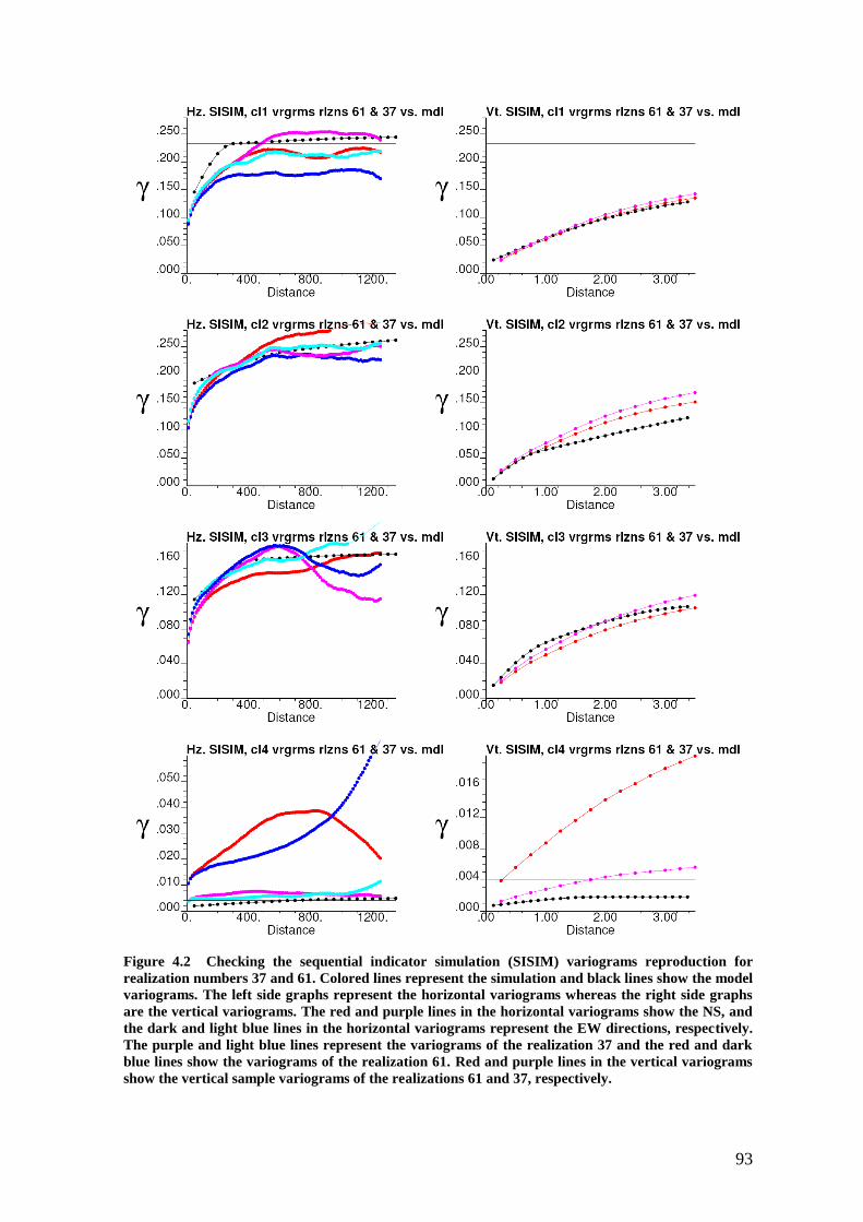
93

Figure 4.2 Checking the sequential indicator simulation (SISIM) variograms reproduction for

realization numbers 37 and 61. Colored lines represent the simulation and black lines show the model

variograms. The left side graphs represent the horizontal variograms whereas the right side graphs

are the vertical variograms. The red and purple lines in the horizontal variograms show the NS, and

the dark and light blue lines in the horizontal variograms represent the EW directions, respectively.

The purple and light blue lines represent the variograms of the realization 37 and the red and dark

blue lines show the variograms of the realization 61. Red and purple lines in the vertical variograms

show the vertical sample variograms of the realizations 61 and 37, respectively.

94

Figure 4.3 Sequential indicator simulation (SISIM) variograms for 100 realizations (red and blue

lines) in horizontal (left graph; red for EW, and blue for NS) and vertical directions (right graphs)

versus model variograms (black lines).

95

4.3.2. The transition-probabilities- reproduction of the SISIM realizations:

The variograms do not have the capability of fully reflecting the interclass spatial

variability dependence structures among pairs of the (soil) classes. Therefore, the quality

of reproducing spatial variability structure could not be evaluated sufficiently for the

simulation results by merely using their indicator variograms. Therefore, it was

considered to plot and evaluate the transition-probabilities (TPs) among the pairs of the

soil classes in principal directions as well to accomplish the spatial variability-

reproduction evaluations.

In this study the TPs of the realizations were compared to their corresponding Markov

chain models. The models of TPs were taken from the TPs and Markov chain model

analyses results which have been addressed in the next chapter.

As the extreme cases, the realizations with the best and worst proportions-reproductions,

i.e. realizations 37 and 61, for the SISIM method were evaluated for their TPs-

reproduction. In other words, it was checked whether or not the TPs of these realizations

correspond to their related Markov chain models?

Similarly, this test was conducted for the realizations produced by the transition-

probability Markov chain (TP/MC) simulation method as well.

Figure 4.4 and Figure 4.5 depict the TPs of the chosen realizations 37 and 61 generated

by the SISIM method. It is clear from these figures that the TPs-reproduction of the

realization 37, in average, was better than that of the realization 61. In general for the

SISIM method, the TPs-reproduction of the realization 37 could be considered rather

reasonable, especially when the emphasis is put on the starting lags of the TPs model. In

the larger lags, the TPs-reproduction becomes weaker.

More details about the spatial variability structure-reproduction have been addressed in

the next chapter.

96

Figure 4.4 The transition-probabilities of the SISIM realizations number 37 (points) and 61 (crosses),

versus their corresponding Markov chain models for the horizontal direction of the existing soil

classes in the study zone. The calculations have been conducted in

97

Figure 4.5 The transition-probabilities of the SISIM realizations number 37 (points) and 61 (crosses),

versus their corresponding Markov chain models for the horizontal direction of the existing soil

classes.

4.4. Three-dimensional sections of the selected SISIM realization:

98

As mentioned above, the realization 37 which represented the best statistical fulfillment

of the minimum criteria was selected as the best realization in terms of the mentioned

criterions.

Moreover, the geological soundness of this realization also had to be evaluated. Hence, a

set of sections were produced in the GOCAD software and were brought here. The

discussions about the geological soundness of this realization, considering the generated

sections have been brought in the next chapter to make it easier to compare the results

from various methods.

Some of these sections have been represented in Figure 4.6 to Figure 4.14.

Figure 4.6 A perspective top view of the realization 37, generated by the SISIM simulation method.

The model represents a 2180m distance in EW and a 1580m distance in NS direction with 15x


99

Figure 4.7 A perspective bottom view of the realization 37, generated by the SISIM simulation

method. The model represents a 2180m distance in EW and a 1580m distance in NS direction with

15x exaggeration in the vertical direction.

Figure 4.8 A perspective top side view of the realization 37, generated by the SISIM simulation



100

Figure 4.9 A perspective bottom side view of the realization 37, generated by the SISIM simulation



Figure 4.10 A top view of the realization 37, generated by the SISIM simulation method. The model



101

Figure 4.11 A top view of the realization 37, generated by the SISIM simulation method showing the

lowermost surface (floor) of the basin. The model represents a 2180m distance in EW and a 1580m

distance in NS direction with 15x exaggeration in the vertical direction.

Figure 4.12 A perspective top side fence-section view of the realization 37, generated by the SISIM

simulation method. The model represents a 2180m distance in EW and a 1580m distance in NS

direction with 15x exaggeration in the vertical direction.

102

Figure 4.13 A perspective top side fence-section view of the realization 37 along the SN direction,

generated by the SISIM simulation method. The model represents a 2180m distance in EW and a

1580m distance in NS direction with 15x exaggeration in the vertical direction.

Figure 4.14 A perspective top side fence-section view of the realization 37 along the EW direction,

generated by the SISIM simulation method. The model represents a 2180m distance in EW and a

1580m distance in NS direction with 15x exaggeration in the vertical direction.

103

5.1. Introduction

The focus of Markov chain models of the transition-probabilities for geostatistical

simulations is the probabilistic quantifying, evaluating, and modeling the changes from

one state to another one in the time or space. Varieties of the states can be considered in

this sense, such as having a rainy day, or a sunny day (in temporal view), or having a silt,

clay, or sandstone along a traverse (in spatial view). Therefore, in the latter example, the

existence of the clay in a point is one state (let say state 1), the existence of the sand is

another state (let say state 2) and so on.

Markov chain (named after the Russian statistician, Andrei Markov) is a sequence of

random variables, X1, X2, X3 … with the Markov property, i.e. the future depends solely

on the present and not on the past. In other words, Markov chain is a sequence in which

the state at one point depends partially, in a probabilistic sense, only on the previous state.

Such a sequence with Markov property has an intermediate behavior between the totally

random and absolutely deterministic sequence (Davis 2002, p. 172). In spatial Markov

chains, the probability of going from one state (e.g. having clay in a point) to another state

(e.g. having sand in the next point) depends solely on the nearest point(s). This Markov

chain is stationary when the mentioned probability, is a function of a separation vector

and not the location of the points (Carle 1999).

In the transition- probability Markov chain (TP/MC) method, the spatial variability

structure is calculated and modeled using the transition- probabilities among various

possible states instead of the variograms (Markovian view to the spatial variation

structure). These transition- probabilities can be molded using a number of models for

Markov chains.

5. Transition-probability Markov chain (TP/MC)

method for modeling subsurface

heterogeneities in Göttingen pilot area, layer 5

104

Figure 5.1 Transition-probabilities: tjk(h)=Pr{ k occurs at x+h| j occurs at x} as a function of

separation vector and not the position in a stationary condition. The blue table summarizes the

numbers of transition (#T) from each facies type to another one in matrix format, for the example of

the facies column in the logs seen at the left side of the figure, for a specific separation vector of zh .

The way of counting the transition for different lag-spacing (red and green arrows here) has been

illustrated in the left-side log column (left graph are modified from Carle 1999, p. 8).

There are good reasons to adopt using the TP/MC approach in estimation stages,

especially when the indicator variogram models demonstrate a considerably vague

variability due to the insufficient sampling rates. In such cases, it would be necessary to

inject more subjective or interpretive information into the model, for instance the mean

length of the geological bodies or the possible sequence or neighboring of the layers.

The advantages of using transition-probability Markov chain approach over the

traditional indicator geostatistical method can be summarized as following:

(a) An easier and improved integration of the geological subjective information of the

facies architecture in modeling spatial variability especially when indicator

variograms give too vague results (e.g. in too sparse or insufficient data-sets).

(b) Producing more consistent patterns with the plausible geology in the outcomes.

(c) Taking all the class inter-relations into account easily. This is especially correct

when it is compared to the alternative methods such as covariograms and

cokriging that demand special requirements in spatial variability modeling,

including some constraints.

(d) Reducing the order-relation violations, in statistical sense of the modeling.

(e) Taking asymmetries into account.

It can be proven that the indicator kriging framework can be reformulated using the

transition-probabilities. It is also possible to prove that the stationary transition-

105

probabilities (in terms of the separation vector) can be fully modeled by an exponential

model and a transition rates matrix like this (Carle 1999):

)exp()( hRhT (5-1)

in which )(hT is he transition-probability matrix of the separation vector h in direction

and R is the transition rate matrix in the same direction.

More details about modeling the transition-probabilities will be explained in the next

sections.

Having the transition-probabilities modeled, one can perform simulations based on them.

More comprehensive descriptions will be represented in the coming sections.

5.1.1. Background

If one counts the number of transition of some states (e.g. a lithology) to the others in an

equidistance traverse and put them in a matrix, it will be called a transition frequency

matrix.

Dividing the row totals of the transition frequency matrix by the total number of

transitions (the complete sum of transition numbers), the relative proportions of the states

will be obtained. The corresponding matrix is called marginal (or fixed) probability

vector (Davis 2002, p. 170).

In many geological investigations, data sequences may be seen that consist of the ordered

successions of mutually exclusive states. For instance, measured stratigraphic sections

have the form of series of lithologies, where the type of lithology or in a drill-hole

through an ore body, the ore and gangue can be considered as states. Observations along a

traverse may be taken at equally spaced intervals or they may be taken wherever a change

in state occurs (embedded Markov chains). Sometimes the nature of the transitions from

one state to another is of main interest rather than the relative locations of the states in a

sequence Davis 2002, p. 168).

According to the conditional probability equations (Davis 2002, p. 170), if the probability

of the occurrence of the states A and B are independent, the probability of occurring state

B at a point given the state A, equals to the probability of the occurrence of the state B:

Pr (B|A) = )Pr(

),Pr(

A

AB =

)Pr(

)Pr(

A

AB =

)Pr(

)Pr().Pr(

A

AB=Pr (B) (5-2)

106

This allows the prediction of, for example, what the transition probability matrix should

look like if the occurrence of a lithologic state at one point in the stratigraphic interval

were completely independent of the lithology at the immediately underlying point. The

expected transition probability matrix would consist of rows that were all identical to the

fixed probability vector.

For comparing this expected transition probability matrix with the actually observed one

to test the hypothesis that all lithologic states are independent of immediately preceding

states, one can use 2 test. For this purpose, first the probabilities should be converted to

expected numbers of occurrences by multiplying each row by their corresponding total

number of occurrences and the expected and observed should be compared values by 2

criterion.

5.1.2. Transition probability-based indicator geostatistics

(1) Objectives and background

As mentioned earlier, because a big part of the geological data is categorical (for

example, lithofacies, soil classes, mineralization phases and so on), indicator kriging

becomes increasingly popular for modeling them. Moreover, some continuous parameters

may represent non-Gaussian behavior which necessitates the use of non-parametric

approaches. However, modeling the spatial continuity which can be considered the most

crucial and difficult practical step in applying the indicator kriging method, may face

serious problems when sufficiently abundant data does not exist. Due to the lack of

enough data in such cases, subjective and interpretative information can fill this gap to

make reliable models. In transition-probability indicator geostatisticsal methods,

proportions, mean lengths (e.g. mean thicknesses), and juxtapositioning patterns (i.e. how

a category locates in space with respect to another category) are used as subjective

information to improve modeling spatial continuity (Carle and Fogg 1996, pp. 453-454).

(a) Some definitions and relations:

The cross-variogram mk (h) of the indicator variables is defined as:

2 mk (h) = E{[ I m (x) - I m (x + h)] [I k (x) - I k (x + h)]} (5-3)

107

where mk (h) denotes the indicator cross-variogram between the categories m and k, I m

(x) and I k (x) are the indicators of the category m and k in location x, respectively., and h

is the lag separation vector (Carle and Fogg 1996, pp. 455). The equation is defined using

the mathematical expectation function.

The cross-covariance C mk (h) is defined as (Carle and Fogg 1996, pp. 455):

C mk (h) = E{ I m (X) I k (x + h)} - E{ I m (x)}E{ I k (x + h)} (5-4)

where C mk (h) is the cross-covariogram between the categories m and k. As applied to

measuring spatial continuity, the transition probability t mk (h) from category m to category

k , is defined in the form f a conditional probability function as (Carle and Fogg 1996, pp.

455):

t mk (h) = Pr{category k occurs at x + h | category m occurs at x} (5-5)

Transition-probabilities are geologically easier to interpret than variograms and

covariograms (Elfeki and Dekking 2001, pp. 569).

The indicator (cross-) variogram, indicator (cross-) covariance, and transition probability

are related to each other as different combinations of one-location marginal probabilities

p k (x) defined as (Carle and Fogg 1996, pp. 455):

p k (x) = Pr{I k (x) = 1} = E{ I k (x)} (5-6)

and two-location joint probabilities p mk (x, h) defined as (Carle and Fogg 1996, pp. 455):

p mk (x, h) = Pr{ I m (x) = 1 and I k (x + h) = 1} = E{ I m (x) I k (x + h)} (5-7)

or (Carle and Fogg 1996, pp. 455):

t mk (h) = Pr{ I k (x + h) = l | I m (x) = 1} = Pr{ I k (x + h) = 1 and I m (x) =l}/Pr{ I m (x) = 1}

(5-8)

Typically in practice, the assumption of a stationary model removes the dependence on

the location x so that:

E {p k (x)} = p k x D (5-9)

In which p k denotes a constant (Carle and Fogg 1996, pp. 455) and

E {p mk (x, h)} = p k (h) x D (5-10)

where p mk (x, h) denotes a joint probability depending only on lag h.

108

Passing the detailed theories, it can be summarized that the cross-variograms and cross-

covariograms can be expressed in terms of the transition-probabilities and proportion, as

following (Carle and Fogg 1996, pp. 456):

mk (h) = p m {t mk (0)- [t mk (h)- t mk (-h)]/2} (5-11)

C mk (h) = p m [ t mk (h) - p k ] (5-12)

In general, it can be demonstrated that the indicator kriging method can be reformulated

using the transition-probabilities.

(b) Methodology

First, two key points regarding the transition probability-based indicator geostatistical

technique deserve mentioning:

(a) Geological and subjective information can be taken into account to improve the

modeling of the spatial continuity of the indicator geostatistical simulation in the

framework of the transition-probabilities indicator geostatistics.

(b) All kriging equations can be reformulated in terms of the transition-probabilities

among the existing soil categories.

Therefore, the method can be performed through the following steps:

1. Estimating and inferring various pieces of subjective information such as proportions,

mean length and juxtapositioning relations.

2. Calculating all the transitions probabilities of the samples between pairs of the classes

(auto- and cross-transitions).

3. Modeling the transitions probabilities using Markov chain models.

4. Solving the related equations and performing the geostatistical simulation.

Carle and Fogg (1996) have discussed this reformulation by detail and represented that

the normal indicator cokriging equation are equivalent to:

109

0...

)(...)(

....

....

....

)(...)(

1

111

mlml

mlNNmlNml

mlNmlml

II

Ixxtxxt

Ixxtxxt

lk

Nlk

lk

,

1,

.

.

.

=

mk

Nmk

mk

I

xxt

xxt

)(

.

.

.

)( 1

(5-13)

(Carle and Fogg 1996, p. 468) and the unbiasedness condition can be expressed as :

klk

N K

l

l pp ,

1 1

(5-14)

in which )( jiml xxt is the transition probability of transition from class m to class l for

the separation vector of )( ji xx , mlI is the identity matrix, 1,lk … Nlk , are cokriging

weights pertaining to the transition of the soil categories from l to k considering the N

nearby estimation points, lp and kp are the proportion of the classes l and k, and

finally lk denotes the KK matrix of the Lagrange parameters (Carle and Fogg 1996, p.

468).

(2) Taking the subjective and geological information into account:

Subjective information such as the proportions, mean lengths, and juxtapositioning

relations can be integrated into the simulation models to improve the modeling of the

spatial continuity. Following, there are some practical points to integrating the mentioned

information in the spatial variability modeling which have been explained briefly here:

(a) Proportions:

Proportions can be deduced directly from the indicator data and conceptual models.

Proportions can be helpful in fitting the sill of a spatial continuity model, whether

expressed in terms of covariogram (C mk (h)), cross-variogram ( mk (h)), or transition-

probabilities (t mk (h)). Equally, the sill of a spatial continuity model entails the guessed

and estimated proportions. Thus, the relationship between proportions and the sill is

connected to subjective development and abstract understanding of the spatial continuity

model.

110

One might be interested in verifying whether or not the sill of a spatial variability model

is acceptable? The frequency of the observations might not be so sufficient to provide an

adequate to make a proper decision about the sill of the spatial variability model so easily.

Conversely, proportions can also be inferred from the sills.

The sill of )(htmk comes near p k , the proportion of category k , whether km or m k.

On the contrary, the sills of kk (h) and C kk (0) come close to )1( kk pp , which requires

solving for "'p'" in a quadratic equation of sill = )1( pp . Then the question would be

about kp whether kp equals kp or 1 - p? The sill of mk (h) and C mk (0) for m k

approaches km pp , an even more ambiguous situation.

The stress on the relationship between proportions and model sills is not to determine

proportions from bivariate statistics (e.g. transition-probabilities), instead to check for

consistency of the spatial continuity model with proportions established by univariate data

and conceptual information. In subjective model fitting of the sill, prior information on

proportions (usually exist) can be applied as a guide for either C mk (h), mk (h), or t mk .

Obviously, among the mentioned measures, t mk (h) provides the straightest relationship

between the model sill and proportions.

(b) Mean Length:

The slope at origin of the graphs of: t kk (h ), kk ( h ) and C kk (h ) is directly related to

mean length (mean thickness) of the soil category k in the direction .

Supposing stationarity for proportions, the mean length of the category k in a direction ,

represented by l ,k , relates to the slope at the origin of kk (h ), C kk (h ) and t kk (h )

by:

h

hkk )0(=

,k

k

l

p (5-15)

h

hCkk )0(=

,k

k

l

p (5-16)

h

htkk )0(=

,

1

kl (5-17)

111

Obviously, mean lengths can be computed directly from continuous data, but not from

discontinuous data.

(c) Juxtapositioning patterns:

As mentioned before, “juxtapositioning” patterns refer to how one category in the space

is located preferentially or non-preferentially in relation to the other one, including

nonrandom and directional-specific (asymmetric patterns) like cycles of fining upwards.

Considering the fact that transition-probabilities are asymmetric, i.e. t mk (h) t km (h),

these patterns also will be reflected in the estimation stage.

An important point in the indictor geostatistics is to ensure that the models conform to

the basic rules of the probability. For example, the estimated probabilities should not be

negative or greater than one, or the estimated probabilities from the indicator (co)kriging

should sum up to one.

(3) Advantages and disadvantages of TP/MC method

Before summarizing the advantages and disadvantages of the TP/MC method, it deserves

mentioning that the literature review for different Markov chain methods revealed an

interesting point. Each author usually had emphasized on the pros of own method without

clarifying its cons. However, a next person who proposed a new method usually criticized

the disadvantages of the previous methods and emphasized again on the advantages of his

own method without mentioning the shortcomings of own technique. Therefore, the

drawbacks of the previous methods could be found in different papers mentioned by the

next authors.

The advantages of transition probability-based indicator geostatistics (TP/MC) over

traditional indicator geostatistical estimation and simulation can be summarized as:

(a) Easier full consideration of the auto- and cross-correlations structure between

pairs of the categories.

(b) Easier integrations of geological subjective information of facies architecture in

modeling spatial continuity (Carle 1999).

(c) More consistency with order relation rules.

(d) Taking the asymmetry in the spatial variability structure of the transition-

probabilities into account to construct more geologically plausible models.

112

While the indicator cross-variograms can not disclose the asymmetry (Carle and

Fogg 1996, p. 463).

(e) In general, in the methods based on Markov chains, the intrinsic non-stationarity

of heterogeneities in larger scales is represented much well (Park 2010, p. 1).

On the other hand, because the TP/MC method follows the same framework as the

indicator geostatistics, it still faces some similar shortcomings as the indicator

geostatistics, for instance:

(a) As represented before, the first stage of the TP/MC method is based on the

reformulation of conventional indicator (co)kriging equations. Therefore, the

order-relation violations can still exist.

(b) Laborious model fitting and a rather long simulation course, because this method

does not apply the Markov approach directly. Specially, the quenching or

optimization stage of the TP/MC simulation to lessen the difference between the

transition probability structures to their corresponding models can be considerably

time-consuming.

(4) Why the TP/MC method was chosen:

In spite of the mentioned disadvantages of the TP/MC method, among the Markov chain-

based techniques reviewed in literature review stage of the present study, i.e. coupled

Markov chain (CMC) and Transition-probability geostatistics (TPG), the later techniques

still had several theoretical and practical drawbacks. For instance, they were not suited

sufficiently for three-dimensional problems and they still did not have available computer

codes or software to use. They were also prone to producing artifacts.

Hence, it was decided to apply the TP/MC scheme while some attempts were made to

improve this technique.

(5) Software:

T-PROGS developed by Steven F. Carle (1999) is a package which enables the user to

apply the transition-probability/Markov approach to geostatistical simulation of

categorical variables. This free package is developed in FORTRAN programming

framework and can be requested from the author.

113

Figure 5.2 an example of (auto- and cross-) transition-probabilities, and relevant Markov chain

models for a two-category facies model of Channel and Not-Channel. Points represent the observed

values, solid curves represent the Markov chain models, dashed-lines stand for the proportions, and

slopes show the estimated slopes from the mean lengths. The graph is taken from Carle and Fogg

(1996, p. 459).

Moreover, a software called GMS, distributed by EMS-I, is a package for modeling

purposes especially for groundwater problems which provides a MS Windows, interface

to T-PRGOS.

5.1.3. The modeling stages in the TP/MC technique

The modeling stages using the TP/MC method has already been explained in the previous

sections.

In this part, some more details are brought about the modeling steps.

Practically, the following were steps taken in this study for simulation of the soil

categories:

(a) Calculating sample transitional-probabilities (i.e. transitions against separation

distance) between pairs of the existing classes in various directions.

(b) Modeling the mentioned transition-probabilities using Markov chain models. Length

statistics can also be considered in this stage to improve the models by integrating more

subjective information or to verify the inferred Markov chain models. Modeling the

transition-probabilities by Markov chain models can be conducted through different

methods. It can be proven that, all the Markov chain models of the transition-

114

probabilities can be constructed using an exponential matrix form like Equation (5-1).

During the modeling of the transition-probabilities using the Markov chain models,

some constraints and conditions should be checked. For example, the auto-transition

rates should be always negative while the cross-transition rates should be positive. The

row-sums and column-sums of the transition rate matrix should obey the Equations (5-

33) and (5-34). The models can be checked for their conformity to the length statistics

(Equations (5-17) and (5-26)), and the general tendencies of the categories to occur

beside or above each other (juxtapositioning patterns and the fining or coarsening

upward or downwards). More detailed discussions about various modeling methods of

the transition-probabilities by Markov chain models are mentioned in the coming

sections.

(c) The Figure 5.3 and

(d) Figure 5.4 represent the calculated and model transition-probabilities among

geotechnical soil classes for horizontal and vertical directions. In this study, although

the observations were considerable and there were no vital need to integrate the

subjective information, the conformity of the Markov chain models of the transition-

probabilities with subjective and interpretive information were also considered. In the

cases where the subjective information were considerably different from their inferred

values from the Markov chain models, the models were adjusted to achieve models

which were more consistent with geological information.

(e) Conducting the simulations using the mentioned Markov chain models and simulation

framework. The simulations here were based on the reformulated indicator (co)kriging

equations using transition-probabilities and Markov chain models.

(f) Further optimization stages (simulated annealing or quenching stages) could be done

using some objective functions. The objective function for performing the simulated

annealing in TP/MC method is defined based on the closeness of the calculated

transition-probabilities of the simulation results to the target Markov chain models of

them. Therefore, in the quenching step of this simulation method, the deviation of the

initial simulation and the target (Markov chain) model is minimized in terms of the

transition-probabilities of the categories, under specific convergence conditions, to

achieve a new improved simulation result. This result should represent a more

acceptable spatial structure in terms of the transition-probabilities reproduction. The

quenching usually improves the geological soundness of the simulated models. In this

115

study, as it will be shown later, quenching improved the geostatistical /statistical and

geological soundness of the simulation results.

5.1.4. Markov chain models of transition-probabilities

Spatial Markov chains, as explained before, stand for a change model in states (e.g. a

sequence of lithofacies in a specific direction) so that the state in a point is dependent

solely on the nearest points but not the others. This spatial Markov chain can be described

based on the spatial probability of changing each state, e.g. a soil type, to the others so-

called transition-probabilities that are dependent only on the separation vector of points

and not the location in the stationary case.

A one-dimensional spatial Markov chain model supposes that the result at the specific

location depends fully on the closest datum. A three-dimensional spatial Markov chain

model conveys that the spatial variability in any one direction can be described by a one-

dimensional Markov chain model (Carle 1999, p. 25).

Even though the Markov chain, in theoretical and mathematical view, is identified very

simply, it has demonstrated considerable applicability in spatial variability

characterization of facies or hydrostratigraphic units in alluvial and fluvial depositional

systems (Carle 1999, p. 28).

Mathematically, it can be shown that the Markov chain consists of linear combinations of

exponential structures, although non-exponential-looking ‘‘Gaussian’’ and ‘‘hole-effect’’

structures can also be generated.

The Markov chain model in the direction can be fully formulated using an exponential

matrix equation like this:

)exp()( hRhT (5-18)

and therefore the Markov chain models can be fully defined having the transition rates.

The transition rates are the change of a transition probability from one state to another in

unit length.

In this equation, h denotes a lag in the direction , and R denotes a transition rate

matrix:

116

,,2,1

,2,21,21

,1,12,11

...

...

...

KKKK

K

K

rrr

rrr

rrr

R

(5-19)

where ,jkr stands for changing rate from category j to category k for each unit length in

direction .

Attention should be paid that the Equation (5-18) do not reflect a plain mathematical

exponential equation but it conveys an eigenvalue analysis procedure since the matrix

exponential is not calculated solely by computing the exponential of matrix elements, that

is, )exp()( ,, hrht jkjk .

Symbolizing R and h by R and h, respectively, for notational simplification, (Rh) can

either be approximated by an infinite series or even preferably with an exact form of:

i

K

i

i ZhRh )exp()exp(1

(5-20)

where i and iZ represent the eigenvalues and spectral component matrixes of R for K

categories, respectively.

To define the term of “eigenvalue” and to keep the mathematical accuracy, the sentences

have been exactly quoted here from Weisstein, E. W. "Eigenvalue." -- from Wolfram

MathWorld, A Wolfram Web Resource (accessed in fall 2011):

“Eigenvalues are a special set of scalars associated with a linear system of equations (i.e., a matrix equation) known also as characteristic roots, characteristics values (Hoffman and Kunze 1971), proper values, or latent roots (Marcus and Minc 1988, p. 144)”. “The determination of eigenvalues and eigenvectors of a system is extremely important issues in physics and engineering. Each eigenvalue is paired with a corresponding so-called eigenvector. If A is a linear transformation represented by a matrix A , is called the

eigenvalue of A with a corresponding vector 0nRX , if there is such a vector X so that:

XAX ” (5-21)

The mathematical details are discussed in the relevant literature (e.g. Agterberg (1974)

and Carle and Fogg (1997) and Carle and others (1998)).

117

An eigenvalue, like i , is inherently zero and is related to a spectral component matrix

having the proportions along each column. Thus, for a four-category system, the

continuous lag Markov chain model written out completely consists of

4,444,434,424,41

4,344,334,324,31

4,244,234,224,21

4,144,134,124,11

4

3,443,433,423,41

3,343,333,323,31

3,243,233,223,21

3,143,133,123,11

3

2,442,432,422,41

2,342,332,322,31

2,242,232,222,21

2,142,132,122,11

2

3321

3321

3321

3321

)exp()exp(

)exp()0.1()exp(

zzzz

zzzz

zzzz

zzzz

h

zzzz

zzzz

zzzz

zzzz

h

zzzz

zzzz

zzzz

zzzz

h

pppp

pppp

pppp

pppp

Rh

(5-22)

In which, the ijkz , are the coefficients of the spectral components matrices iZ calculated by

the eigensystem analysis (Carle 1999, p. 30).

Hence, the Markov chain model for every element of )(htij in )(hT equals to a linear

combination of the K-1 exponential categories plus the column category proportion. For a

four-category case, this can be expressed as following (Carle 1999, p. 30):

)exp()exp()exp()( 44,33,22, hzhzhzpht ijijijjij (5-23)

The Markov chain model for in TP/MC method can be established using different

methods such as; discrete lag Markov chain method, maximum entropy, transition

frequencies, embedded transition frequencies, and embedded transition-probabilities.

“The lateral extent of the 3-DMarkov chain model output by MCMOD1 must be finite,

with limits that consider statistical closeness. Kriging-based algorithms, which do not

consider cross-correlations, easily rank statistical closeness by the magnitude of the

variogram (or covariance) model or a prescribed search radius with anisotropy ratios.

However, the ranking of a full cross-correlation matrix for multiple categories is not so

straightforwa”(Carle 1999, p. 30).

The determinant as a closeness measure is used not only in the MCMOD program of the

T-PROGS software to rank the statistical closeness in MCMOD program but it is also

1 A program in T-PROGS software to find a proper Markov chain model for transition-probabilities.

118

used in the search and simulated quenching algorithms of the TSIM program (in the T-

PROGS software).

It can be shown that the determinant of the transition-probability matrix )(hT would be

the product of its eigenvalues )(hk (Carle 1999, p. 30):

K

k

k hhT1

)()(det (5-24)

More details about the eignsystem analysis can be found in relevant literature (e.g. Carle

1999, pp. 27-28).

Two- or three-dimensional Markov chain models can be achieved by accepting the

assumption that the spatial variability in every direction can be characterized using a 1-D

Markov chain model. The 1-D Markov chain models in each direction can be achieved by

interpolating the 1-D Markov chain models in principal direction models. Similar

conclusion can be made about the transition rates based on the assumption that the

transition probability matrix can be fully determined by the use of the transition rates

matrix (Carle 1999, p 30).

A brief description of each Markov chain transition probability modeling method is

explained following:

(a) Transition rates:

When the transition rates, which equal to the slopes of the transition-probabilities at the

origin, can be inferred directly (for example from the transition probability graphs of the

input data) or from subjective information such as mean lengths and interpretations of the

facies successions, this technique could become a suitable choice.

In addition, in the case that the rough initial transition rates are inferable from another

Markov chain modeling (e.g. discrete-lag method) and analysis method, the transition

rates can be adjusted and fine-tuned to achieve better fits in the next stages.

(b) Discrete-lag Markov chain model:

If a transition probability matrix )( hT is multiplied successively by itself at lag h , the

Markov chain model can be formulated using the discrete-lag method.

It can be shown that, the transition-rates matrix can be formulated as following, in this

technique (Carle 1999, p. 27):

119

h

hTR

)(ln (5-25)

which contains the eigensystem analysis. More details about the eigensystem analysis can

be found in the relevant literature.

Therefore, one can use this method to produce the Markov chain models that honor the

calculated transition-probabilities from input data in specific unit lags, for example, in

one-, two-, three-, or n-unit lags.

This method is usually applied in the initial steps of Markov-chain modeling to obtain a

rough estimation of the models and transition rates.

In this case, the Markov-chain models of transition-probabilities were initially made

based on discrete-lag method. Different lags were to tested to find the model that fits the

best to all of the observed transition rates while fulfills the statistical requirements of the

model such as negative auto-transition rates and positive cross-transition rates. Checking

the debugging file, it could be evaluated whether or not the models had statistical

problems and in the necessary cases, there were modified.

In this study, in most cases, a 3-lag (discrete-lag) Markov chain model was considered as

the initial transition rates Matrix approximation step.

(c) Transition-probabilities of embedded Markov chain analysis:

Embedded transition-probabilities are defined based on the probabilities of the transitions

among the categories where the states are changed. Therefore, there are no auto-

transitions, in embedded Markov chain analysis.

Embedded Markov chain analysis provides the most interpretive framework in Markov

chain modeling. Therefore, it can be applied in the case of sparse data or even no data

(Carle 1999, pp. 35-36).

For example, the relation of the embedded transition-probabilities, mean length and

transition rates can be expressed as following:

zi

zij

zijL

r,

,

, (5-26)

where zijr , stands for the transition rate from category i to category j, zij , is the embedded

transition probability from category i to category j, and ziL , indicates the mean length of

the category i, all in vertical direction.

In addition, the following condition also should be met:

120

11

,

K

j

zij (5-27)

in which, K is the total number of categories.

In addition, interpretations and subjective information, inferred from embedded

transition-probabilities, can be used to check and verify the chosen Markov chain models.

The embedded transition-probabilities, stored in the debugging file of the MCMOD

program of T-PROGS software, can be interpreted for some subjective information such

as the tendency of categories to occur above or beside each other and the mean length of

each category in specific directions for example in vertical direction that would be the

mean thickness of each category.

In general, a category with the highest frequency is considered in T-PROGS software as

the background category. Besides, since in the embedded transition-probabilities analysis

there are no auto-transitions, the inference of embedded transition-probabilities is not too

difficult by integrating subjective information in Markov chain modeling of the transition-

probabilities.

(d) Transition frequencies of embedded Markov chain analysis:

In an embedded Markov chain transition-probabilities analysis, the numbers of transitions

are indicated at the first step. For example, the count of transitions from soil class 1 to the

soil class 2 and to all other classes are determined to calculate the transition-probabilities

from class 1 to all other classes. Here, again, there are no auto-transitions. With

normalizing the matrix of the number of counts by the sum of the whole matrix, the

transition frequencies are calculated. If these counts are normalized by the row totals, the

transition-probabilities will be achieved. The application of transition frequencies rather

than transition-probabilities is suitable in the evaluations of statistical independence.

(e) “Independent” or “maximum entropy” (disorder) Markov chain analysis:

If there are no tendencies in the occurrence of any category over or beside the others, the

conditions of the “independence” or maximum entropy should be met.

“The disorder of the juxtapositional tendencies in a particular direction, say , can be

quantified by the entropy S of bed-to-bed transition frequencies ,jkf , the probabilities

that one bed occurs next to another, by”:

121

j k

jkjk ffS )ln( ,, (5-28)

It can be proved that in the Maximum-entropy conditions, the transition rates can be

obtained by:

jk

zjkzj

MaxS

zjkMaxS

zjk

fL

fr

,,

)(

,)(

, (5-29)

5.1.5. TP/MC simulation technique

TP/MC simulation is performed in two stages:

(a) The initialization stage:

In this step, a method similar to the sequential indicator simulation (SISIM) algorithm

(explained by Deutsch and Journel 1998, pp. 125-127, p. 149-150) is applied, except that

this technique uses a transition probability-based indicator cokriging to approximate the

local conditional probabilities:

Pr{k occurs at 0x | )(xi j ; KjN ..2,1,...2,1 }K

j

jkj

N

wxi1

,

1

)( (5-30)

In above equation (Equation (5-30)), the parameters definitions of the equation can be as

summarized following:

N: data number in the neighborhood, i: indicator for category j, ,jkw : estimation weights

for transition from the state j to the state k, and is the index of the points applied in the

estimation of the conditional local probabilities (Carle 1999, p. 47).

Estimation weights ( ,jkw ) can be calculated from solving Equations (5-13) and (5-14).

The only point is that, in the mentioned equations, estimation weights have been denoted

as instead of w .

Implementation of transition probability-based cokriging, improves the consideration of

spatial interclass cross-correlations.

122

(b) Simulated annealing:

Simulated annealing or quenching is an optimization stage. A more detailed description

of simulated annealing method for geostatistical analyses can be found in Deutsch 2002

(pp. 275-294) as well as in Deustch and Cockerham 1994. In this stage, initially generated

configurations using a transition probability-based SISIM technique, are improved and

optimized to enhance the agreement between measured and modeled transition-

probabilities. In other words, the difference between the Markov chain models of

transition-probabilities and the calculated transition-probabilities of the simulations are

decreased.

Thus the attempt in quenching step is to solve the optimization problem of

})()(min{1 1 1

2K

l

K

j

K

k

MODljkSIMljk hthtO (5-31)

where O denotes the objective function, lh represents the l=1,…, M indicated lag-

vectors, j and k show the K existing categories, and finally “SIM” and “MOD”

distinguish the simulated (measured from the realization) and model transition-

probabilities, respectively (Carle 1999, p. 53).

In each simulated point, the neighbouring states are cycled and the transition-probabilities

are calculated. An objective function is defined as following:

O = E {(Transition probability of simulation- Transition probability of model) 2 } (5-32)

If the perturbation minimizes the objective function (O), it is accepted and otherwise it is

rejected.

In this case, considering the mentioned soil classification scheme, due to rather enough

amounts of data-points, considering the length statistics has no significant effect on

improving the Markov chain models, although in fewer data, it would be more effective

and useful for sure. The discrete-lag method and inferred proportions were first used to

make the MC models, they were checked for statistical accordance, and then the models

were further examined using the length statistics.

123

5.2. Transition-probability Markov chain (TP/MC) geostatistical modeling of geotechnical data-set in Göttingen test site

5.2.1. Overview:

To perform a transition-probability Markov chain geostatistical simulation and analyses

of geotechnical soil-classes model in Göttingen test zone, the first step, as argued before,

was to calculate the transition-probabilities among different classes in various directions

from input data. Similar to the sequential indicator simulation (SISIM) and indicator

kriging (IK) modeling methods, the transformed coordinates system was applied in

transition probability Markov chain-based analyses. These transition-probabilities (auto-

and cross-transitions) were calculated and plotted for horizontal (Omni-directional

horizontal) and vertical directions.

The next step was to find a suitable Markov chain model that not only fit the transition-

probabilities of the input data but also it could fulfill some basic criterions. These

criterions have been summarized following:

(1) The auto-transition rates should be minus.

(2) The off-diagonal transition rates should not be negative.

(3) The row sums for transition rates matrix should be zero (Carle 1999, p.

29):

01

,

K

k

jkr (5-33)

(4) The column sums, considering the proportions of the categories, must

conform the following equation (Carle 1999, p. 29):

01

,

K

j

jkjrp (5-34)

(5) The transition rate values should individually be reasonable values.

All the mentioned criterions are checked internally in the MCMOD program of T-

PROGS software and reflected in a debugging file.

The first step in finding the proper Markov chain model which could fulfill the

mentioned criterions and fit the sample transition-probabilities acceptably started with

discrete-lag Markov chain modeling. In discrete-lag Markov chain method, the model

124

honors the transition-probability data in a specific (discrete) lag. In other words, the

model passes through a transition probability point in a specific lag, e.g. second-lag of

transition probability plot, which has been calculated from the sample data.

One can choose the first-, second-, third- or a bigger number-unit lag transition

probability point depending on the spatial structure of data which produces the best fit

while no errors in MCMOD debugging file.

As Carle and Fogg (1997) have suggested, the Walther’s law of facies succession

(Leeder 1982, p. 122) can be applied as a practical means to infer the horizontal

transition-probabilities structure of a sedimentary succession from its vertical-direction

structure and vice versa. Walther’s law of facies succession (in the absence of non-

conformities) implies that the vertical succession of sedimentary environments reflects

their lateral structure (Leeder 1982, p. 122).

Hence, an observed fining upward asymmetry in the vertical transition-probabilities

might be incorporated to construct the fining outward model in the dip-direction transition

rates (Carle and Fogg 1997, p. 908).

The next step usually is to improve the Markov chain model using embedded Markov

chain method. In the embedded Markov chain modeling where the embedded transitions

are considered, the length statistics and other interpretive information can also be taken

into account. Embedded transition probability Markov chain modeling method is in

general more flexible and interpretive. In the case of this study, the Markov chain

modeling of transition-probabilities started with discrete-lag modeling (3-lag), followed

by embedded Markov chain method and finally using the transition rates to improve the

models using the adjustment of transition rates.

The produced models in MCMOD program were checked by plotting the data transition-

probabilities and Markov chain models in the same graph. Figure 5.3 and

Figure 5.4 represent the data transition-probabilities and the chosen calculated models for

vertical and horizontal directions.

In the MCMOD program the operator defines the Markov chain model type, categories

proportions and the relevant model parameters as well as input data file. Then the

program produces five output files as the elements of Markov chain model. Three files are

the transition-probabilities of Markov chain models in x, y, and z directions respectively.

These files are used in plotting and checking the produced Markov chain models

compared to the transition probability of the input data. These three files have the ASCII

file format. Therefore, the strategy for checking the models is to plot the transition-

125

probabilities of model(s) and those of data in a same plot and comparing them together as

mentioned above. Then, the debugging files were checked for their conformity to the

required conditions. The graphs always do not change significantly but the debugging file

may show better conditions with required fine-tuning of the Markov chain models to

fulfill the necessary conditions.

The two other files which include the three-dimensional Markov chain model are in

binary format. One of the two mentioned files is the three-dimensional model file and the

second file is determinant file which contains the statistical closeness data (see Section

5.1.4 for more details about the method).

After choosing, adjusting and improving the three-dimensional Markov chain transition

probability models, regarding the debugging file of MCMOD program and transition

probability graphs, one can also perform some length statistics checks to improve or

verify the existing model, especially in the case of insufficient data. In the case of lack of

enough information, the length statistics can play an important role to fill the information

gap in order to approximate the proper Markov chain models or improve them.

In this study, due to the existence of sufficient samples and data, the application of length

statistics did not seem to be necessary.

126

Figure 5.3 Transition-probabilities of the four geotechnical soil categories in vertical direction

calculated from input data (dots) and their corresponding Markov chain model (solid lines) from

transition rates method as a final fine-tuned model.

127

Figure 5.4 Transition-probabilities of the four geotechnical soil categories in horizontal direction

calculated from input data (dots) and their corresponding Markov chain model (solid lines) from

transition rates method as a final fine-tuned model.

128

5.2.2. Some points about using post-quenching phase in TSIM program of the T-PROGS software:

To perform the TP/MC simulations, termed here as TSIM simulation, the TSIM program

of the T-PROGS software was applied. There were some practical points and

considerations in the applications of this program in the present study which has not been

explained here to avoid too much discussions and details. In this section, a summary of

the most essential points of these points have been addressed.

For the reasoned explained before, the TSIM simulations started with generating

simulations without quenching steps. Then, every further quenching step was performed

on the available simulations of the previous stage. However, the TSIM program conducts

these quenching steps on the same output file of the available simulations from previous

stage(s) by assigning a negative number for the quenching steps. Therefore, the existing

simulation as well as output files (which give a summary of each simulation round) had to

be copied first and renamed for the next stage. Copying the simulation files was for

preserving the existing simulation results and renaming was for applying the last

simulation results for the next quenching step with different names to avoid replacing the

existing files. Since, the simulations were recorded in different files but there was only

one generic “tsim.out” file for each round, the proper renaming had to be done on the

output files in each step. To make it also easier to calculate the variograms of all the

TSIM, simulation, the realizations of each TSIM simulation were merged into one file

with compatible format of the GSLIB software. Scripting was applied during this study to

make several handlings and calculations easier or even feasible.

5.3. Evaluating the TP/MC simulation results and their underlying models

5.3.1. Overview:

To evaluate the simulations produced by transition probability-based Markov chain

method, some interpretive and statistical criterions were employed and suggested in this

study.

The purpose and meaning of the produced simulations evaluations and their underlying

models was to assess the goodness of applied models for TP/MC simulations, improve

129

them if necessary, and suggest the best produced realizations in terms of mentioned

criteria. In addition, the proper criterions were sought to compare the results out of

different geostatistical simulation methods and evaluate how reliable in general these

criterions were.

Oy Leuangthong et al (2004, p. 72) have summarized the minimum acceptance criteria

for geostatistical realizations. Based on their suggestions, the following criteria to

evaluate the qualities of produced simulations and choosing the best ones have been

considered in this study:

(a) Honoring the input (i.e. conditioning) data at their locations.

(b) Histogram (or proportions) reproduction.

(c) Transition probability Markov chain models reproduction (as a measure for

spatial variability structure).

(d) Variogram reproduction (as another spatial structure measure).

(e) Geological soundness of the produced model.

Actually, the criterion of TPs-reproduction has not been suggested by Oy Leuangthong et

al (2004). However in this study, the application of TPs-reproduction as another spatial

variability measure has been suggested to improve the evaluation of the spatial variability

structure, especially to evaluate the interclass transition structures. In particular, TPs-

reproduction criterion could match better to the TP/MC method which essentially relies

on modeling the TPs as spatial variability structure measure and using Markov chain

models.

More details about and the results of each mentioned criterion have been explained

further, in the coming sections.

5.3.2. Honoring the input (conditioning) data values at their locations or data reproduction:

It is a known fact that (co-)kriging is an exact estimator, so that the estimate at a data

location equals exactly to the input data value. In other words, if kriging estimation is

performed at the location of a data point, the result would exactly be the same as input

data value at that location and the estimation variance will be zero:

),(* uzzk ,uu n,...,1 (5-35)

130

where *

kz represents the kriging estimation value of the random variable, Z, at location u

and )(uz stands for the data value at location u .

Considering that initial stage of the applied simulation methods was based on

reformulated (co-)kriged estimations and their corresponding estimation variances to

define the local conditional cumulative distribution functions (CCDF), the applied

simulation methods also had to reproduce the data exactly at their locations. However, in

practice, for some reasons, few data points were not reproduced. For example, in some

simulation algorithms that assign data points to the simulation grid nodes, in order to

speed up distance calculations, some input data may not be reproduced. For that reason,

the total number of assigned data may become less than the total number of available

conditioning data. This phenomenon can happen probably because of one of the following

reasons:

1. The sample coordinate may be situated outside of the limits of three-

dimensional model (simulation) grid (Figure 5.5, A).

2. The data point may be inside the limits of 3D simulation grid, but it is trimmed

or there is no variable available (Figure 5.5B).

3. If there are more than one data points available inside the 3D simulation grid

limits near to a simulation grid block and one of samples is closer to the block

center, the closer sample will be kept and the other sample will be ignored

(Figure 5.5, C).

Figure 5.5 a schematic illustration of how the input data may not be assigned to the simulation grid

node: A, the sample exists but it is located outside the simulation grid; B, the existing sample is inside

the simulation grid but the value is trimmed; and C, samples exist and are inside the simulation grid

but there are more than one samples inside the grid block but only the closest sample is assigned (the

graph is taken from Leuangthong (2004, p. 133).

131

In WinGslib software, the user can decide to let or not let the SISIM program to assign

the data to the model nodes. The assigning of the data to the simulation model nodes can

be chosen to reduce the simulation run-time. In this case, the decision was to let the

SISIM program of WinGslib software to assign the data to the simulation nodes to speed

up the simulation procedure. In addition, some data points could also be trimmed in the

SISIM program. Therefore, it was expected that a number of input data points would not

be reproduced (Leuangthong 2004, p. 133).

Figure 5.6 input data conditioning errors histogram of SISIM simulation method for realization

number 20.

Input data reproduction can be checked in different ways. Oy Leuangthong et al (2004,

pp. 133-134) have suggested the use of cross-plots in order to assess the goodness of

input data reproduction. However, since this approach is not well-suited for categorical

attributes, another solution was adopted here to facilitate the evaluation of conditioning

data reproduction for each realization. A MATLAB code was developed to compare the

observed and simulated soil categories and assess the conditioning-data reproduction ratio

in all sample points in the simulation models. This check was performed for all

realizations generated by various simulation methods. For this purpose, in each step the

mentioned MATLAB code reads the soil category of a data point from borehole data file

and finds the soil category in its nearest simulation point of a realization from its

corresponding simulation file. Then, the code compares the observed and simulated

categories from these two points with calculating their differences. Finally, the ratio of the

correctly conditioned simulation points in each realization (with the difference values of

132

zero), was calculated for all realizations. The MATLAB output was copied and stored in a

text file separately for each simulation method. The conditioning data reproduction can be

evaluated afterwards. This difference also could be represented in a conditioning-errors

histogram. The error then is the difference of the observed category values of wellbore

data and their corresponding simulated category in their nearest points. Ideally, this

histogram should only contain zero values (100% of the frequency) that would mean the

exact reproduction of all input (conditioning) data points. In practice, however, some

errors are expected. Figure 5.6 represents an input data conditioning error histogram of

the realization number 20 for the SISIM simulation method. The histogram is quite

symmetric with a governing frequency on no errors, meaning that the input data

reproduction was almost perfect except for a minor portion of data points. Some errors in

this method also could occur due to the imperfect match of the simulation and data points.

For instance, if a data point is located between two simulation points with exactly similar

distances from data point, the computer code will consider the first point in the simulation

file.

In simulation number 20 of the SISIM method, the 99.64 % of input data was exactly

reproduced.

The results show that the input data reproduction of the SISIM realizations were in the

range of 99.47% and 99.88% that is nearly perfect for all realizations. The same checks

were performed on the realizations of different TSIM methods.

The conditioning on input data for the TSIM method is also about 89.47% to 95.22%

which seems also fairly acceptable but weaker compared to the SISIM method.

Since it was not possible to represent all the conditioning-errors histograms of all the

realizations of different simulation methods, the qualities of input data reproduction was

evaluated solely with the ratio of exactly conditioned simulation points in which the

conditioning-errors were exactly zero.

Table 5.1 summarizes the simulations conditioning on the input data for different

simulation methods.

The clear conclusion from this table could be that, the conditioning-data (input data)

reproduction can be accepted for the realizations of all utilized simulation methods in this

study. However, the conditioning on the input data has clearly been reduced by adding the

number of quenching steps. Since the reduction of the input data honoring with further

quenching steps is unfavorable whereas the extra quenching steps increase the other

statistical and geological qualities of the simulations, a compromising decision could be

133

made to keep a good input data reproduction as well as an acceptable simulation at the

same time. Therefore, it can be suggested that the number of quenching steps should not

be too much but at the same time it should not also be too few.

Table 5.1 The table represents a summary of honoring (conditioning on input data) for various

geostatistical simulation methods.

Simulation method Ratios of correctly conditioned input data

Statistic SISIM TSIM without

any quenching steps

TSIM with two quenching

steps

Based on the all input data points

Minimum 0.9947 0.923 0.8863

Maximum 0.9988 0.9431 0.9277

Arithmetic mean

0.9979 0.9329 0.9103

Satadard deviation

0.0011 0.0064 0.0120

Based on the accepted input data points in the

simulation program

Minimum 0.9947 0.9318 0.8947

Maximum 0.9988 0.9522 0.9366

Arithmetic mean

0.9979 0.9418 0.9190

Satadard deviation

0.0011 0.0064 0.0121

5.3.3. Histogram- (or proportions-) reproduction:

(1) Introduction:

One of the least requirements for a realization of a geostatistical simulation to become

acceptable, in statistical sense, is its ability to reproduce its expected representative

134

histogram of the attributes under study. The target attribute in this study was the soil

categories. Hence, a realization that, its histogram of the studied attributes, deviates too

much (beyond an acceptable tolerance) from the target distribution, is rejected for

histogram reproduction. In such cases, either another realization that fulfills this criterion

better can be selected for further evaluations or the underlying models of the simulation

should be adjusted to achieve a more suitable set of results which reproduce the target

histogram better. Even, it could also be necessary to choose a different simulation method

to achieve more proper simulation results that better reproduces the expected histogram. It

should be reminded here that, the primary geostatistical models in this study were initially

improved, prior to the geostatistical simulations. For the kriging-based method of SISIM,

the cross-validation, and for the transition-probability-based method of TSIM, the

Markov chain model parameters control was applied to improve the initial models which

were implemented later for geostatistical simulations. About the transition-probability-

based methods, the debugging files were checked for the accordance of the simulation

models statistics to the necessary statistical conditions such as non-negative cross-

transition and negative auto-transition rates in the transition-rates matrix. More details

about the necessary conditions of the TP/MC simulation models have already been

discussed in the relevant section.

Two essential points should be kept in view when evaluating the quality of histogram

reproduction for a realization of a geostatistical simulation:

(a) A number of proper criterions should be chosen to verify the closeness of the

histograms of the soil categories in realizations to that of the reality as well as

to assess how close these distributions are and which realization reproduces

the real distribution better.

(b) The practical limitations and suitability as well as available software should be

considered

The application of the Q-Q plots could be considered as one of the most common

techniques in histogram reproduction evaluations of geostatistical realizations of a

simulation method. A Q-Q plot, in fact, compares the distributions of the two sample

groups. For instance, in the case of histogram reproduction tests of the geostatistical

simulations, the realizations versus the expected (target) distributions can be compared

with each other. This method is especially suitable to be implemented when evaluating all

the realizations at once. In such cases, the Q-Q plot of all realizations versus the input

135

data is plotted to compare the distributions of these two sets. If the Q-Q plot (roughly)

follow the 45-degree line of the y=x, it means that the two distributions, i.e. the

simulations and the expected one in this case, are almost identical. Still, this technique is

better suited for the continuous data-sets rather than the categorical ones and especially in

assessing all the realizations at once. Besides, the calculation and plotting of such huge

point-sets, due to a high computational demand, is rarely feasible. For example, in this

application, the GSLIB and R programs exceeded their (memory and run-time) limits.

Thus, the application of Q-Q plots was not preferred for the proportions-reproduction test

in this project. Consequently, an analytical alternative was preferred for testing the

histogram reproduction of such a categorical attribute, particularly because of offering a

clearer index to evaluate and compare the results by such an analytical measure.

To approximate the target distribution, in this study, the application of the volumetric

proportions of the categories inferred from the borehole data considering the vertical

grids-transformation corrections could be applied. This suggestion was supported by

similar cases in the literature such as Ritzi et al. (2007) as well as in Deutsch and Journel

(1998), and the discussion in Section 2.1.6. To achieve a modified representative

histogram of the soil categories, the effect of the grids transformation in vertical direction

had to be considered. In addition, due to the existence of some clustering in boreholes

locations, corrections such as cell- or polygonal-declustering seemed necessary. The

declus program in GSLIB software can be used for a cell-declustering of the input data.

Both the mentioned methods including the declustering and direct proportions

calculations from boreholes data with corrections for vertical grids-transformation were

applied separately here to estimate the representative global proportions. Then, the results

of these two methods were compared with each other. Nevertheless, there are still three

important points about these corrections:

(a) The applied declustering algorithm depends very much on declustering

parameters that affect the global histogram approximation.

(b) When these two methods to estimate the global histogram were applied

separately, the results out of them were almost equal. As stated before, the first

method was cell-declustering technique and the second approach was the

volumetric proportion calculation from the borehole data just with considering the

correcting weights proportional to the effective-range of samples in vertical

directions in the transformed space. Therefore, in the second technique, the weight

of each sample in the calculation of the proportions in global distribution was

136

higher in the thinner parts of the layer where there were less number of samples,

and lower where the layer was thicker and the number of samples was more.

According to the conducted cell-declustering of input data, the global proportions

of the soil categories from two methods were more or less similar.

(c) When performing the ordinary kriging algorithms, the declustering is not

necessary because the ordinary kriging algorithm, automatically and effectively

corrects the clustering effect (Deutsch 2002, p. 50). However, for the geostatistical

simulations, a representative histogram in which the clustering problem has been

modified is greatly necessary.

In this study, as mentioned above, the estimated global distribution of soil categories

calculated by declustering method and from input data with vertical grid-transformation

corrections were not considerably different. In addition, the declustering parameters were

also affecting the estimated histogram. Therefore, the application of the second method

which was easier and more consistent has been suggested for similar cases. Yet, the

locally varying proportions and the proportions estimation uncertainties as well as the

conceptual or deterministic process-based models or the secondary information such as

seismic measurements could also be taken into account for a better proportion estimation

of soil categories. The reason of the suitability of the second method, i.e. inferred from

boreholes data with corrections related to the grid-transformation, for the proportions (of

categories) estimation, was due to the plenty of available samples as well as the lack of

significant trend in the proportions variations over the study area in the transformed-grid

space.

Hence, in this study, a realization was not rejected for the histogram reproduction when

its proportions of the categories were close-enough to those of the expected ones

(considering the acceptable tolerances). This evaluation had to be clearly supported by

statistical concepts. Moreover, another insight to the proportions reproduction evaluation

could be that both boreholes data and simulations should reflect the same populations

which closely imitate the distribution of existing categories in the reality, all in the

transformed space. Taking such an insight into consideration for this problem, the chi-

square statistical homogeneity of populations test was also suggested to assess the

proportions reproduction in this case.

137

(2) The proportions-reproduction criteria:

Considering the above discussion, two decisive factors were suggested in this study to

evaluate the proportions-reproductions of the realizations of each simulation method;

first, a chi-square test for homogeneity of populations, and second, the deviation rate of

the observed from expected proportions together with a chi-square-like statistic that will

be explained more in the coming sections which has been named here as sum of the rates

of squared deviations. This measure has been defined according to the squared deviation

of the observed from expected proportion relative to the expected proportion which is

defined similar to the definition of the normalized mean square deviation statistic. In

addition, the chi-square ( 2 ) statistic for homogeneity of proportions test was also

applied to assess the proportions-reproduction in the realizations and rank them in terms

of its goodness. The ranking of the realizations in terms of the chi-square statistic for the

quality of proportions reproduction, was based on the fact that, the lower the 2 value,

the closer the distribution of that realization should be to the expectation, because

the 2 statistic reflects the departure of the observed frequencies from the expected ones.

There are also further statistical measures for the evaluation of the accordance of the

realizations and target (real) distributions in a simulation method, such as Kolmogrov-

Smirnov goodness of fit test for the continuous parameters or the RMS (root mean

square) statistic for the categorical data (e.g. Clausen (1982, p. 55) for RMS).

a. Proportions-reproduction check using a deviation rate framework:

To evaluate the quality of the proportions-reproduction, a criterion has been suggested

here which has been referred as the proportions “deviation rate” (D.R. or DR). This rate

seems comparable to the framework of the mean absolute percentage error (MAPE) or

mean absolute percentage deviation (MADE). However, the difference between these two

methods is that, the DR is evaluated for each category separately and the greatest

emphasize is considered on the most dominant classes. MADE is applied in evaluation of

the model fitting in time series. The deviation rate of the proportion of category i in a

realization, has been defined in terms of the ratio of the deviation of the proportion of a

category (i.e. category i, in this case) from the expected (i.e. global) proportion:

iE

iEiO

iP

PPRD

)(

)()(.. (5-36)

138

where iRD .. , for a realization of a geostatistical simulation, is the deviation rate of the

observed proportion of the class i from its expected proportion, iOP )( is the observed soil

category proportion of the class i in the mentioned realization , and iEP )( is the expected

proportion of the same (global proportions).

It should be emphasized again that the proportions of the soil categories inferred from the

boreholes, taking the grid transformation corrections into account, were regarded as the

target distribution in the “deviation rate” calculation here.

In the proposed framework, the deviation rate of the proportions of soil categories

( ..RD ) for each realization of a simulation method was evaluated, starting the evaluation

from the proportion of the soil category with the highest observed frequency in the

boreholes (after necessary modifications related to the grid-transformations) and ending

to the least frequent soil category from input data. Hence, a more emphasize was put on a

class with the highest expected frequency and then, the second highest expectedly

frequent class, and so forth. The practical steps of this method were as following:

(a) First of all, the proportions of soil categories in the realizations were extracted

from simulation output files and put in a table that besides, included the expected

proportions of the categories.

(b) Next, the deviation rates for each category were calculated using the above

formula (5-36).

(c) In the third step, the deviation rates which were not greater than the maximum

acceptance limit, e.g. 0.1 (=10%) or 0.05 (=5%), were determined and indicated.

The key classes for evaluation of the deviation rates of the proportions were the two

most, and three most expectedly dominant classes in the SISIM (classes 2 and 1),

and TSIM (classes 2, 1, and 3) methods, respectively. The maximum accepted

deviation rates were 0.1 (10%) for the SISIM method and 0.0025 (0.25%), or at

times, 005 (5%), for the TSIM methods. The reason for considering a much lower

acceptable deviation rate limit for the TSIM methods were because of much closer

proportions to those of the target in the realizations of the TSIM methods. The

signification of the acceptable deviation rates were by assigning a “1” when it was

acceptable and a “0” otherwise.

(d) Then, the realizations representing the acceptable deviation rates for the first

two, or in some cases, first three expectedly most dominant soil classes were also

indicated.

139

(e) The indicated realizations pointed out in step (4) were selected as realizations

with acceptable proportions reproduction.

(f) These selected realizations were sorted then, in terms of a statistic which looks

like a chi-square statistic but has been defined somewhat differently and has been

named in this study as the sum of the rates of squared deviations (SRSD). As

mentioned before, this measure has been defined according to the squared deviation

of the observed from expected proportions relative to the expected proportion.

Actually, this measure has been defined similar to the coefficient of the variation of

the mean square deviation statistic or the chi-square statistic. The difference of this

measure with the coefficient of the variation of the mean square deviation is that

there is no averaging in SRSD and the normalization is done against the expected

values for each squared deviation but not the total mean of the observed

(proportion) values. In this sense, SRSD is more similar to the chi-square statistic.

However, the observed and expected values should be in terms of counts in the chi-

square statistic while the observed and expected proportions are employed in SRSD.

Therefore, the SRSD was defined (proposed) in this study in somewhere between

the chi-square and the coefficient of the variation of the mean square deviation. The

aim of defining such a measure was to bring a complementary measure to highlight

the absolute differences (by squaring the deviation) relative to the expected value

(by dividing by its expected value) and summing these normalized deviations.

However, there is no standard table for this statistic and it can only be used to

compare among the different simulations to rank them for their quality of

proportions-reproduction. The analytical definition of the SRSD has been brought in

the next lines. The selected realizations were sorted in terms of their SRSD rates

statistic of the proportions in an ascending order. The best realizations in terms of

the proportions-reproduction should represent the least sum of the SRSD value as an

indicator for the closeness of the simulation proportions to those from corrected (for

the grid transformations in the vertical direction) observations in the boreholes.

Hence, wherever these deviation rates in a realization, for the two or three first

expectedly most dominant classes, were in an acceptable range, let’s say, 0.1 or 0.05, the

related realization was accepted and otherwise declined.

For instance, if the two classes that expected to be most predominant soil categories were

considered as a basis to evaluate the quality of proportions-reproduction, let’s say, class j

and class k (which were respectively classes 2 and 1 in this research) and the maximum

140

acceptable deviation rate is aRD .. , then the acceptance criterion could be expressed as

following:

{( jRD .. < aRD .. ) and ( kRD .. < aRD .. )} the realization is acceptable in terms of the

quality of proportions reproduction.

The reasons for suggesting such a framework were:

(a) Methods that could not be implemented or were not adequate: The Q-Q plot was

not applicable in such cases not only due to software limitations but also for its

incompatibility to the purpose of the categorical attributes evaluations. Moreover,

the chi-square test of homogeneity does not always seem capable of identifying a

satisfactory proportions-reproduction adequately. As an example, regarding the

expected proportions of the categories (i.e. the target distribution), the 2X statistic

(as a calculated estimation of the 2 statistic) for the homogeneity of proportions test

suggested the realization number 20 as the best proportions-reproducing realization

for the TSIM-without-quenching-step simulation method, whereas the calculated

proportions of the realizations 161 and 12

2, putting more emphasize on the most

dominantly observed classes in the input data, have obviously closer distributions to

that of the target. In part (b), it will be explained why the belief here was that

putting more stress on the most anticipated classes was a sensible decision. It has

already been explained why the proportions of the soil categories inferred from the

input borehole data were regarded a proper estimation of the real ones in this case.

In addition, the chi-square method is not straightforward in terms of the departures

from the expected proportions. Actually, a better decision could be made with a

criterion that expresses these deviations more directly, for example in terms of a

deviation rate. Moreover, the chi-square statistic for test of homogeneity, usually,

gives a single overall value for all proportions-reproduction elements (proportions-

reproduction of cl1 to cl4). Nevertheless, one can also evaluate each single chi-

square element for each soil category separately, to compare the expected and

realization proportions.

1 The proportions of the soil classes 1 to 4 for the realization 16 in TSIM method without any quenching

step were 0.3672, 0.4255, 0.2015, and 0.0059 while the expected proportions were 0.372, 0.423, 0.201, and

0.004, respectively. 2 The mentioned proportions for realization 12 for the same method were 0.3730, 0.4185, 0.2024, and

0.0060 while they were 0.3618297, 0.4317658, 0.2028174, and 0.003587139, respectively for realization

20. Clearly, both the realizations 16, and 12 represent closer proportions to those of the target ones for soil

classes 1, 2 and even 3.

141

(b) More reliable statistics in bigger classes: It is expected that the soil classes with

the highest observed proportions, deduced from the borehole samples (considering

necessary corrections for to the grid-transformation), would have the most reliable

estimation of their proportions compared to the smaller classes. This is because of

two reasons. First, the more dominant classes (based on the borehole data) have

larger sample numbers and hence more reliabilities in their statistical inferences.

The second basis could be that they also cover expectedly larger geometric sizes

compared to the average spacing of the borehole samples, especially in the

horizontal direction. Since the less observed proportions and hence the less

coincidence of the boreholes with the smaller classes is due to their smaller

geometric sizes compared to the average sample spacing, and vice versa. Therefore,

the proportions of the small classes are prone to be approximated more inaccurately

while the approximated proportions would be more reliable for the bigger classes.

Hence, putting more emphasize on the reproduction of the proportions of the bigger

soil classes is a sensible decision. In addition, in a volumetric view, if the

proportions of the largest classes could be reproduced better, the volumes of the

other classes also would not depart too much from their expected total volumes.

This is because the total volume of the all categories is a fix amount for each of the

realizations. However, if the volumetric deviations of the smaller classes are

evaluated with a ratio rather than their volumes (similar to what is done in a chi-

square test or by deviation rates), the deviations may seem very considerable. For

example, because the expected volume of the soil category 4, is 0.004 according to

the categories proportions inferred from the borehole data considering the grid-

transformation corrections, while the simulated volumetric proportion of the

category 4 is 0.006 in a realization, there will be about 50% deviation of the

proportion of this soil category from the expected value whereas the absolute

volumetric difference is not so high. Besides, it is more probable that the

approximated proportion of the category 4 (from the input data) is not that accurate

and reliable due to the very low number of available samples from this class. The

horizontal geometric sizes of this category should also obviously be much less than

the boreholes spacing. However, for more frequent classes (in the boreholes

samples), less variations should be acceptable, since their inferred proportions from

the input data should expectedly be more precise. As a result, the suggested

stepwise proportions deviation rate framework, that combines two insights of the

142

overall and fractional volumetric deviations from the expectations and puts more

merit on the most anticipated classes, seems a more proper solution for the

proportions-reproduction evaluation problem. In fact, this scheme forces the

absolute volumes of the soil classes to be reproduced much closer to those of target

and therefore to the real ones. In addition, the deviation rate is more straightforward

in representing the extent of the deviation from the expected proportions.

In this insight, as cited above, the most important and reliable soil-classes for the

evaluation of the proportions reproduction are the classes 2, and 1 for the SISIM method,

and classes 2, 1, and finally 3 for the TSIM method(s). The reason is that, these classes

have the highest expected proportions and frequencies. Hence, the realizations that their

proportions deviation rates of classes 2, and 1 (as well as class 3 in the TSIM method)

from their expected proportions were less than 0.25% for the TSIM methods (except for

the TSIM with two post-quenching-step method where the acceptable rate of 0.5% was

considered), and less than 10% for SISIM method, were adopted as the acceptable

realizations of these methods, in terms of the proportion- reproduction. As pointed out

above, for the TSIM method with two post-quenching steps, the maximum acceptable

deviation rate of 0.5% was considered because the deviations were, in general, higher for

the results of this method compared to those of the TSIM methods with other numbers of

quenching steps (i.e. no-, 1-, 3-, and 4-post-quenching steps). The maximum acceptable

deviation rates for each simulation method were chosen so that the two or three best

proportions-reproducing realizations could be differentiated. The reason for considering a

lower acceptable value for maximum deviation rates in the TSIM with two-post-

quenching-step method is that, none of the realizations in this method have the deviation

rate of the 0.25%.

Table 5.2 summarizes and compares the results of the selected realizations produced by

different simulation methods. The selection and comparison of the realizations in terms of

proportions-reproduction was based on the two different mentioned methods of deviation

rates (defined and proposed by the author of this dissertation) and chi-square test of

homogeneity.

It should be clarified here that the proposed statistic which has been called the “sum of

the rates of squared deviations” (SRSD) of the proportions here, was defined as

following:

)(/)()(1

2

i

k

i

ii EPEPOPSRSD (5-37)

143

in which )( iOP is the observed proportion of the category i, and )( iEP is the expected

proportion of the category i. Squaring the term )()( ii EPOP , makes the observed and

expected proportions value positive and intensifies this difference while dividing the

squared difference generates a rational value that compares this intensified positive

difference to the expected proportions. SRSD resembles a chi-square statistic in some

ways. Hence, SRSD facilitates the differentiation of better proportions-reproduction more

clearly with a simpler calculation scheme compared to that of the chi-square test of

homogeneity.

b. Proportions-reproduction check using the chi-square test of homogeneity:

Since, the real proportions of the soil categories are not exactly known and their inferred

proportions form the boreholes are not necessarily accurate approximations of the real

proportions, the consideration of the proportions inferred from the input data may not

necessarily be accurate-enough in proportions-reproduction evaluations. Thus, the

application of the chi-square test of homogeneity was suggested here as an alternative

solution.

The chi-square statistic, in general, is defined as following:

ii

k

i

i EEO /)( 2

1

2 (5-38)

where the2 is the chi-square (or chi-squared) goodness of fit statistic, iO is the observed

frequency (counts) for the bin (category) i, iE is the expected frequency for the bin i (i.e.

the reference frequency for the bin i or let say the expected count for category i), and k is

the existing number of categories (McKillup and Darby Dyar 2010, pp. 234-236).

The problem of chi-square goodness of fit test here was that the sample sizes of input and

simulation data were dramatically different. For that reason, another method had to be

opted with the capability of comparing the proportions of the categories rather than their

frequencies (counts).

It is a common question in earth sciences that the proportions of the considered categories

in two or more groups of samples come from the same population or not? In contrary to

the chi-square goodness of fit test, there are no expected frequencies or proportions of the

categories in such problems. However, the chi-square test of homogeneity examines if the

proportions of the categories in the two sample groups, i.e. the proportions observed in

the boreholes versus the proportions calculated in the simulations, are heterogeneous that

144

means they come from two different populations or they are homogenous and come the

same population. The observed frequencies (counts) can be calculated simply by

multiplying the observed proportions by the total number of their corresponding sample

numbers (number of simulation nodes). The expected frequencies also can be calculated

by a similar method, i.e. multiplication of the expected proportions by total number of

data samples. It should be reminded again that, in the calculation of the proportions and

the frequencies of the categories in simulations, corrections should be implemented due to

the application of a transformed space.

The chi-square statistic for the test of homogeneity can be defined as following (Online

source: “Chi-Square Test of Homogeneity.” Chi-Square Test of Homogeneity, AP

Statistics Tutorial. StatTrek.com1; McKillup and Darby Dyar 2010, pp. 234-236):

c rN

c

crcr

N

r

cr EEOX1

,

2

,

1

,

2 /)( (5-39)

where 2X is the calculated chi-square statistic2, rN is the number of data rows that

indicates the number of sample groups (here rN =2, i.e. two sample groups of ; the

boreholes data, and simulation result), cN =k=4 is the number of categories, crO , is the

observed frequency of data in row r, and column c (in the contingency table), which is the

data frequency of sample group r (e.g. in borehole data; r=1, and in a simulation result;

r=2) for category c (i.e. soil classes 1, 2, 3, and 4; c=1, 2, 3, 4), the crE , is the expected

frequency of data in row r, and column c, or the data frequency of sample group r for

category c. The row and column here, respectively, stand for the row and column of a

contingency table (McKillup and Darby Dyar 2010, pp. 234-236). Using the 2X symbol

instead of 2 is because 2X is a calculated or estimated value for chi-square statistic.

The expected frequency counts are computed separately for each population at each level

of the categorical variable, according to the following formula:

n

nnE cr

cr, (5-40)

1 "Chi-Square Test of Homogeneity." Chi-Square Test of Homogeneity, AP Statistics Tutorial.

StatTrek.com, Stat Trek Website. Web. Summer 2011. <http://stattrek.com/ap-statistics-

4/homogeneity.aspx>.

145

where crE , is the expected frequency count for the population r at level c of the

categorical variable, rn is the total number of observations from the population r, cn is the

total number of observations at sample group c, and finally n is the total sample size

(Online source: “Chi-Square Test of Homogeneity.” Chi-Square Test of Homogeneity, AP

Statistics Tutorial. StatTrek.com1).

Therefore, the null hypothesis (H0) states that the proportions of all of the categories in a

realization and those of the boreholes have come from the same population with the

significance level of whereas the alternative hypothesis (HA) says the contrary at least

for one of the categories.

The null hypotheses will be rejected if the calculated chi-square ( 2X ) is greater than the

critical chi-square values function (2

),( DF ) or the calculated p-value is less than the

significance level of , for at least one of the categories:

2X >2

),( DF (5-41)

valuep < (5-42)

where 2

),( DF stands for the chi-square critical value function with the DF, degrees of

freedom and a significance level of (Online source: “Chi-Square Test of

Homogeneity.” Chi-Square Test of Homogeneity, AP Statistics Tutorial. StatTrek.com2).

This critical value can be derived from the standard chi-square distribution tables or chi-

square calculators having the significance level ( ) and the degrees-of-freedom (DF).

The degrees of freedom for homogeneity of proportions test is calculated as following:

1)-1)(N-(NDF cr (5-43)

where rN , and cN are the numbers of columns, and rows in the contingency table,

respectively. In other words, as an example in this study, rN =2 is the number of sample

groups that should be evaluated for being homogenous with one another (i.e. derived from

1 "Chi-Square Test of Homogeneity." Chi-Square Test of Homogeneity, AP Statistics Tutorial.


4/homogeneity.aspx>. 2 "Chi-Square Test of Homogeneity." Chi-Square Test of Homogeneity, AP Statistics Tutorial.


4/homogeneity.aspx>.

146

the same population), and cN =4 is the number of columns in this table which is the

number of existing categories. Therefore, the degrees-of-freedom for the present study is:

3311)-1)(4-(21)-1)(N-(NDF cr (5-44)

In this case, k is the number of soil classes. It is clear from the definition of 2 that the

smaller the 2X (estimated 2 ), the closer the evaluated simulation proportions to those of

the reference will be (“Chi-Square Test of Homogeneity.” Chi-Square Test of

Homogeneity, AP Statistics Tutorial. StatTrek.com).

(3) The proportions-reproduction checks in the test site:

The distributions were calculated and checked for the different realizations of the SISIM,

and TSIM (transition-probability Markov chain simulation) methods including the TSIM

simulation without quenching steps, as well as the TSIM simulations with one-, two-,

three-, and four-step post-quenching phases. The proportions of the categories in each

realization of the various simulation method were obtained from their corresponding

debugging (*.dbg), and the generic “tsim.out” files. To avoid missing the produced results

in the “tsim.out” files, in the TSIM method(s), the “tsim.out” files of the TSIM program

from T-PROGS software were renamed, prior to running any new simulation. For

example, here, they were renamed to the files with the prefixes names, the same as the

output realizations file names, and the suffixes of “_out.out”.

In the” post-quenching” steps, the simulated annealing is conducted on the previously

generated realizations of various simulation methods. The post-quenching steps were

conducted to reduce the differences between the transition-probabilities of a simulation

and the target Markov chain models of them. Thus, the “post-quenching step” term was

applied here for the further quenching steps performed on the available realizations from

the previous stages. The mentioned available realizations could be the product of the

realizations with or without further quenching steps from the previous stages (mainly

about the TSIM method). In fact, in each stage, only one quenching step was added to the

previous realizations. Therefore, the TSIM simulations were started by conducting the

TSIM simulation without any quenching steps, then a quenching step was performed on

the realizations of the previous stage (i.e. on the TSIM method without any quenching

step) to result the TSIM realizations with one quenching step, then another quenching

147

step was performed on the result of the previous stage (i.e. on the TSIM with one “post-

quenching step”) to achieve the TSIM realizations with two post-quenching steps, and so

on.

Table 5.2 Comparison of selected realizations produced with different simulation methods for

proportions reproduction using two different suggested histogram reproduction test methods

Realizations with acceptable proportions-reproduction

Simulation method

Based on deviation rates

(maximum acceptable deviation rate)

Based on chi-square test of homogeneity

SISIM (Sequential Indicator Simulation method)

12, 38, 37 (0.1)

37, 12, 65

TSIM without quenching (Markov chain simulated annealing optimization) steps.

16, 12, 1, 20 (0.025)

20, 16, 12, 1

TSIM with 1-post-quenching (Markov chain simulated annealing optimization) steps.

19, 12, 18, 4 (0.025)

7, 6, 19, 12


12, 3, 16, 9 (0.025)

19, 16, 11, 17


9, 4, 12, 1 (0.025)

3, 16, 9, 11


19, 18, 16, 17 (0.025)

19, 18, 16, 15

The reason for using the “post-quenching” technique was to save the simulation time by

avoiding the repetitions of quenching stages. For example, to achieve a TSIM simulation

with a three-step post-quenching, one can simply carry out a quenching step on the

realizations of a TSIM simulation with two post-quenching steps, which was actually

produced by performing a quenching step on the realizations of the one-step post-

quenched TSIM simulation, and so forth.

Table 5.2 summarizes the proportions reproduction test results of the geostatistical

simulations. The table includes the accepted realizations for all applied simulation

techniques based on the two stated proportions-reproduction test methods.

(4) The density of the simulation grids:

148

In this study also, the effect of using coarser grids on the proportions reproduction was

tested. As it has been expected, the results were dependent on the grid sizes so that each

grid size lead to a different proportions-reproduction quality. Stepwise application of the

different grid sizes is actually a part of the multiple-grid simulation strategy embedded in

the GSLIB simulation programs to improve the simulation algorithm by taking the long-

range structures into account. This strategy however, has not been included in the TSIM

program of the TPROGS. The multiple-grid simulation concept is to perform the

simulation in two or more stages; i.e. starting from the coarser grids to the finer ones. In

other words, a coarser grid is simulated first. Then this coarse grid is used as the

conditioning data for another finer-grid simulation and so on (Deutsch and Journel 1998,

p. 190). One of the advantages of using the multiple-grid strategy is that it leads to a

better reproduction of the long-distance variogram structures. Therefore, adding this

strategy to the TSIM program of the TPROGS could also be suggested to enhance the

efficiency of the TSIM algorithm for a better spatial structures reproduction.

The number of realizations in different simulation methods:

It should be reminded here that the number of realizations for the TP/MC (transition-

probability Markov chain) method was less (i.e. twenty realizations) than those of the

SISIM method (i.e. one hundred realizations). There were two reasons for generating only

twenty realizations in each of the TSIM simulation rounds:

(1) Technical limitations: The technical limitations, because of exceeding the

capacity of the TSIM program for such a big and fine-resolution simulation grid

(nx=175, ny=124, nz=28; with unit cell size of mmm 25.05.125.12 ) from its

limits after producing twenty realizations. Even by improving some capacity

settings and parameters of the program, the TSIM program exceeded its limits.

Perhaps, this capacity could still be enhanced. Due to the limited Ph.D. time,

further enhancements were not followed up at this moment.

(2) Low variations in TSIM method results: A considerably lower variations was

observed among the realizations of a TSIM method compared to those of the

SISIM method, in terms of several statistical criterions such as proportions of the

soil categories, variograms, and transition-probabilities of the realizations (see the

proportions-reproduction tables as well as the TPs and indicator variograms-

149

reproduction in this section). Then, adding more numbers of realizations would

not add a significant merit to the analysis, even if the technical limitations would

not be encountered. (Yet, a set of 20 realization of the SISIM method was

produced and checked for their indicator variogram spectrum. As Observed in

these results, they covered nearly the same variation spectrum of the variograms.

However, due to much higher variations of SISIM compared with the TSIM

method, I preferred to keep 100 realizations for the SISIM method (see Figure 6.1

and Figure 6.2).

(5) More details about the chi-square test for homogeneity of proportions:

As it has already been explained in this context, the chi-square statistic for the

homogeneity of populations test was calculated for each of the realizations produced by

various simulation methods.

In order to formulate the proportions reproduction of the realizations for each simulation

method using the chi-square homogeneity of proportions test, the null and alternative

hypotheses and the significance level (the critical p-value) should be defined. The

significance level ( ) is the probability of improperly rejecting the null hypothesis (H0)

and in general, the null hypothesis is the hypothesis of “no difference” or “no effect”

(McKillup, Steve, and Darby Dyar 2010, p. 13). In this problem, the null hypothesis is

that the proportions of each soil category and those inferred from the borehole data (with

necessary corrections explained in Section 2.1.6) reflect samples from the same

population.

The critical p-value (or significance level of ) for selecting the four and three best

realizations, for TSIM, and SISIM methods, respectively, was considered as a criterion to

evaluate the proportions reproduction qualities among different simulation methods. For

instance, if for the simulation methods of A and B, the significance levels for selecting the

four best realizations are A and B , respectively, A can be compared with B to

analyze and decide which method have reproduced the target proportions better. In this

example, if A > B , it can be concluded that the realizations produced by method A,

could reproduce the real proportions better. In other words, the method A, worked better

in terms of proportions reproduction in this example.

150

To evaluate the simulations using the 2X values for the proportions reproduction in this

stage, the significance levels with which, in each simulation methods, the three best

realizations in SISIM method and four best realizations in TSIM method(s)1 could be

selected, were suggested. The reason for selecting a less number of realizations as the best

proportions-reproducing ones in the SISIM method was that, this method had

considerably lower proportions reproduction quality compared to that of the TSIM

method and the quality of the realization would drop dramatically if a more number of

realizations were selected. Lower critical p-values were selected for the simulation

methods with a less quality of proportions reproduction (e.g. SISIM or TSIM without

quenching step methods) and higher critical p-values were selected for the simulation

methods with a better quality of proportions reproduction (e.g. TSIM methods with one or

more numbers of quenching steps). It was concluded that, performing additional

quenching steps, in general, improved the proportions reproduction quality of simulations.

Although after the first quenching step, in the TSIM with two-post-quenching steps, the

proportions-reproduction became even slightly worse. Then, it did not change

significantly in three-step post-quenching stage. However, the proportions-reproduction

was improved considerably in the four-step post-quenching phase. Moreover, in all the

TSIM methods, the suggested critical p-values are considerably above the conventional

significance level of 0.05. Therefore, with the significance level of 0.05, none of the

selected realizations of the TSIM method could be rejected. Yet, a significance level of

0.15 (15%) could be suggested for all of the selected realizations. Even in this

significance level, all the accepted realizations (i.e. four best realizations in each TSIM

method) fall in the statistical level of not being rejected for the TSIM methods.

Sorting the realizations in terms of their 2X homogeneity statistics in an ascending order,

the realizations with the least estimated chi-square values ( 2X ) were located on the top of

the list, representing the realizations which best reproduce the target proportions.

(6) Summarizing the results of the chi-square test of homogeneity to evaluate the

goodness of proportions-reproduction:

Table 5.3 summarizes some descriptive statistics of the chi-square values for the

homogeneity of proportions of the realizations (with the boreholes data), generated by

1 When the term “TSIM methods” has been implemented in this context, the aim was to refer to the

application of the TSIM method with different post-quenching steps.

151

different simulation methods. The minimum, maximum, average, and the standard

deviations of 2X corresponding to each of the simulation methods are reflected in this

table. In addition, the related p-values for each of the 2X statistic together with the

corresponding coefficient of variation of the standard deviation of 2X have been placed

in the parentheses.

The mentioned descriptive statistics were chosen to represent the statistical location and

dispersion of the calculated chi-square ( 2X ) values.

Table 5.3 Summary of chi-square statistics for different simulation methods applied in this study.

Simulation method

Statistic

2

minX

(corresponding

2minX

P )

2

maxX

(corresponding

2maxX

P )

2

averageX

(corresponding

2averageX

P )

Standard deviation of

2X (corresponding

coefficient of variation)

TSIM without quenching (Markov chain simulated annealing optimization)

steps.

0.888135 (0.8282)

33.35429 (2.7112e-7)

8.584887566 (0.0353)

8.124094 (0.946325)

TSIM with 1-post-quenching (Markov chain simulated annealing optimization)

steps.

0.018947599 (0.9993)

0.79631175 (0.8503)

0.313639749 (0.9574)

0.245226 (0.781872)


steps.

0.189506385 (0.9792)

0.896819433 (0.8261)

0.428922857 (0.9342)

0.217569 (0.507245)


steps.

0.344708282 (0.9514)

0.693566396 (0.8747)

0.500907457 (0.9186)

0.091308 (0.182285)


steps.

0.000510806 (0.9999)

0.840421978 (0.8397)

0.20874874 (0.9761)

0.281918 (1.350514)

SISIM (sequential indicator

simulation method)

8.51003149 (0.0365)

138.6058825 (0)

48.8278298 (0)

22.84308 (0.467829)

These results can be summarized and interpreted as following:

152

(a) In general, the TSIM realizations reproduce the soil categories distribution (i.e. the

proportions) much better than those of the SISIM method. In the SISIM method,

the average of the calculated chi-squares is 2

averageX =48.82783. The 2X ranges

from 8.5100 to 138.6059 for different realizations whereas the 2X has the overall

average of 2.0074, and ranges from 0.0005 to 33.3543 for the TSIM method. The

decision that which simulation could reproduce the proportions better was based

on the fact that the lower the 2X , the better the proportions-reproduction.

(b) In all of each TSIM methods, the majority of realizations (for example, 12

realizations out of 20 in the TSIM without-quenching-step method) reproduce the

proportions adequately with the significance level of 5%. In addition, all of the

realizations of the TSIM method(s) with quenching steps reproduced the soil

proportions with the significance level of 80% or better and most of the

realizations (at least 12 out of 20 realizations) reproduced the proportions with the

significance level of at least 90%. Therefore, it can be concluded that the quality

of proportions-reproduction was notably higher in all of the TSIM methods

especially in the TSIM method with quenching steps.

(c) Only three realizations of the SISIM method fell in an acceptable range with the

significance level of 1%. The best realization of the SISIM method (i.e. the

realization number 37), reproduced the proportions at the significance level of

3.65% which is just under the usual acceptance significance level of the chi-square

tests (5%). Hence, the proportions-reproduction quality in the SISIM method was

generally poor especially compared to that of the TSIM methods.

(d) Adding the quenching (or post-quenching) steps to the TSIM method increased

the proportions-reproductions significantly. However, the quality of the

proportions-reproductions did not increase regularly with the increasing of the

numbers of quenching steps.

(e) Paying attention to the TSIM with four quenching steps, nearly all of the

generated realizations (17 out of 20 realizations) reproduced the proportions with

a 90% significance level. Thus, the proportions-reproduction was the best in TSIM

153

simulation with four quenching steps, based on the chi-square test of

homogeneity. In addition, the selected realizations from both the chi-square

homogeneity and the deviation rates test (proposed by the author of this

dissertation here) were more common for the TSIM with four-post-quenching

steps. A lot of common selected realizations between two methods of deviation

rates and chi-square test of homogeneity while with a less computational costs and

complexities for the former bedsides the best accuracy of the realizations in this

simulation method (based on the proportions-reproduction tests), suggested that

the deviation rates framework could be efficiently applied in the similar problems

for proportions-reproduction checks. More details about this method and its

analogues statistical method has been addressed in part (2)a, section 5.3.3 from

Chapter 5. Perhaps, some conditions should be taken into consideration before

applying the proportions deviation method such as the enough number of input

sample data. It seems that inferring an accurate-enough representative histogram

from the input data is the key point in the application of the deviation rates

method.

Regarding the fact that the two proposed proportions-reproduction tests, here, suggested

different but with many common and similar selected realizations, it can be concluded

that the two methods lead to the similar results. The two methods of the proportions

“deviation rate” and the chi-square test of homogeneity for evaluating the proportions-

reproduction of the realizations are suggested to be applied to the similar cases where the

categorical variables are being simulated. In addition, the proportions deviation rate

scheme with a simpler framework can be applied in the similar problems leading to more

or less similar results.

Table 5.4 illustrates the two methods of the proportions reproduction test (“proportions

deviation rates” and the chi- test of homogeneity) for the realization number 37 of the

SISIM method as an example. The “Global proportion” column is the proportions

calculated from the boreholes considering the necessary grid-transformation corrections,

the “Calculated proportions” come from the calculation of the proportions of the

realization number 37 of the SISIM method obtained from the simulation debugging file,

and the next columns show the relevant calculations.

154

Table 5.4 Illustration of the calculations frameworks of the chi-square test of the homogeneity of

proportions, and deviation-rate, for the realization number 37 of the SISIM geostatistical simulation

method.

Soil class

Global proportion

Calculated proportion

Element 2X

realizations

Element 2X

boreholes

Total 2X

Deviation rate

Was the deviation rate<=0.1

?

Cl1 0.372 0.3486 0.007193 2.5877

8.5100

0.0629 1

Cl2 0.423 0.4189 0.000165 0.0593 0.0097 1

Cl3 0.201 0.2258 0.012846 4.6211 0.1234 0

Cl4 0.004 0.0061 0.003387 1.2183 0.5250 0

5.3.4. Transition-probabilities-reproduction:

The transition-probabilities-reproduction of the generated simulations by different

simulation methods reflects how close or similar the transition-probabilities (TPs) of the

simulations to their corresponding MC models were. This test was implemented as a

spatial variability index to verify one of the minimum acceptance criteria for geostatistical

simulations. As discussed before, variograms were the other spatial variability tools

applied in this study to asses the quality of generated realizations as one of the minimum

criteria for accepting each realization. The variograms-reproduction of the realizations has

been discussed in the coming section. In this section, the focus is on the evaluation of the

transition-probabilities as another spatial variability tool to assess the spatial-variability-

reproduction of realizations. The author proposes here, to consider the transition-

probabilities reproduction as another minimum acceptance criterion of any realization in

similar problems since the transition-probabilities capture the spatial variability structure

of the categories, in terms of the change of state of each soil or facies category to any

(other or the same) state. Therefore, the transition-probabilities of the simulations should

reflect some spatial variability features better than what variograms can. It has been

proposed here to apply the both variograms and transition-probabilities to assess the

spatial-variability-reproductions of the generated realizations.

155

Regarding the fact that there were lots of realizations from different geostatistical

simulation methods and different simulation parameters (such as the number of quenching

steps in the TSIM method), it would practically be extremely tedious to compare the

transition-probabilities of all the simulation results one-by-one (e.g. by plotting them in a

graph or performing an analytical comparison) with their corresponding Markov chain

models. The technical limitations regarding the software also were required to be

considered. To overcome these problems, two strategies could be considered:

(a) To assess the acceptability of each realization separately, the realizations which

reproduced the soil proportions the best were selected at the first step. Then,

these selected realizations were suggested to be checked for their transition-

probabilities- reproduction (abbreviated here as TPs-reproduction) in the next

step. One of the good reasons to evaluate the proportions-reproduction initially

was that, a realization with closer proportions to those of the model would be

expected to show closer variogram and transition-probability sills to those of the

model. The reason for this prospect is that, the expected sill of an indicator

variogram ( )1( ppc ) or a TP is a function of the proportion of that soil

category (i.e. kp ). It is worth reminding again that, the sill of )(htmk is tangent

to the kp (proportion of category k ) line at the infinity, whether km or m

k. Therefore, an acceptable proportions-reproduction can, at least, ensure a

better sills-reproduction for variograms and TPs. It was shown before about the

SISIM method that, the realizations with poorer proportions-reproduction

demonstrated, in general, a weaker variograms-reproduction while the

realizations with a better proportions-reproduction, represented commonly, a

better variograms-reproduction as well. Hence, it can be expected that, the

realizations which reproduced the target proportions better, should also be

capable of better reproducing the spatial variability including the TPs. Figure 5.7

to Figure 5.16 represent the TPs of the best selected realizations (in terms of

their proportions-reproductions)from TSIM method versus their corresponding

TP Markov chain models. Therefore, a better TPs-reproduction was also

expected in addition to a better variograms-reproduction, of the selected

realizations. The TPs-reproduction of the selected realizations seems acceptable

and better for the simulations with some quenching steps. Obviously, it should

be considered that the effect of a better proportions-reproduction on the better

156

TPs-reproduction should be in a specific extent. Because, if the general image of

the patterns become similar, the proportions also would be similar. However, in

general, a better proportions-reproduction can not completely guarantee a better

variograms- or TPs-reproduction. Ideally, a sequential geostatistical simulation

should reproduce the spatial variability structure (variograms and TPs) of the

simulation model. Yet, in practice, the outcome of the sequential geostatistical

simulations can not really reproduce the variograms or TPs because of the

limitations embedded in the algorithms. The most important factor which affects

the variograms/TPs reproduction is the long-range variations (Zanon and

Leuangthong 2005). According to Zanon and Leuangthong (2005), having a

more abundant data-set and using the multiple-grid search strategy can improve

the long-range-variation-reproduction of the sequential simulations.

Nevertheless, in general, choosing the best proportions-reproducing realizations

can narrow the range of realizations which should be evaluated for its

variograms-/TPs-reproduction efficiency by suggesting the more acceptable

realizations.

(b) To assess the overall efficiency and quality of all the realizations of a simulation

method, one could also calculate the average transition-probabilities of all

realizations of a geostatistical simulation method and plot them together with

their corresponding Markov chain models in one plot and compare them with

each other among different methods. Similarly, the average indicator variograms

of all realizations of a simulation method could also be calculated and plotted

together with their relevant indicator variogram models, to evaluate the overall

efficiency of a simulation method for its variograms-reproduction. These

evaluations were initially attempted by the author using a special trick (i.e.

constructing a big three-dimensional dummy model made by all the realizations

of each simulation method which includes the grids of all of the realizations

while the spatial continuity measures of the new model have the same value as

that of the overall average of all realizations). However, this procedure was not

accomplished further because the evaluations using the first method and plotting

of the variograms and TPs of all realizations of each method in a graph seemed

sufficient and even more efficient. Hence, only the results of first method have

been brought and discussed here.

157

As mentioned above, the transition-probabilities of the best realizations, chosen in terms

of their proportions-reproduction, and their corresponding Markov chain models were

plotted at the same graphs and compared with each other to evaluate the transition-

probabilities reproduction. The selection of the best realizations, in terms of the

proportions-reproduction was a compromising decision between the results of two

different proportions-reproduction-test methods of the chi-square test of homogeneity,

and the deviation rates frameworks.

As Figure 5.7 to Figure 5.16 represent, the TPs of the selected realizations match their

relevant Markov chain models, in general, more or less well. This match was better for

the TSIM methods, especially for the TSIM simulations with some quenching steps.

However, the match between the TPs of the realizations and those of the models were

weaker in vertical direction, especially for the class 4 which had the least observations

frequency. These interpretations had been obtained by a graphical comparison of the

transition-probabilities of the realizations and models. It has been explained in the coming

section that, there are some analytical frameworks suggested in a number of literature to

evaluate the variograms and other statistics-reproduction for simulation evaluations by

analytical methods. However, it has been shown there, why the application of these

measures was not suitable in this case so that the graphical method was preferred. Further

attempts can be suggested to develop and suit similar analytical criterions to evaluate the

generated realizations.

158

Figure 5.7 Horizontal transition-probabilities among the soil classes for realization 16 generated by

TSIM without any quenching step method (dots) and corresponding Markov chain models (solid

lines).

159

Figure 5.8 Vertical transition-probabilities among the soil classes for realization 16 generated by

TSIM without any quenching step method (dots) and corresponding Markov chain models (solid

lines).

160


TSIM method with a one-step post-quenching phase (dots) and corresponding Markov chain models

(solid lines).

161


TSIM method with a one-step post-quenching phase (dots) and corresponding Markov chain models

(solid lines).

162


TSIM method with a two-step post-quenching phase (dots) and corresponding Markov chain models

(solid lines).

163


TSIM method with a two-step post-quenching phase (dots) and corresponding Markov chain models

(solid lines).

164


TSIM method with a four-step post-quenching phase (dots) and corresponding Markov chain models

(solid lines).

165


TSIM method with a four-step post-quenching phase (dots) and corresponding Markov chain models

(solid lines).

166


TSIM method with a four-step post-quenching phase (dots), corresponding Markov chain models

(solid lines), and realization 37 generated by SISIM method (cross symbols).

167


TSIM method with a four-step post-quenching phase (dots), corresponding Markov chain models

(solid lines), and realization 37 generated by SISIM method (cross symbols).

For the TSIM method without any further quenching steps, the realization number 4 was

selected because of its best proportions-reproduction. For this realization, the TPs usually

168

reach a plateau, quicker than the model (Figure 5.7and Figure 5.8). The TP sills are also often

different with the model. In this case, the number of near the origin points falling on or very

close to the model line, is not so many, especially for the vertical direction. According to the

Figure 5.9 and Figure 5.10, with a further quenching step in the TSIM method, the number of

mentioned points (falling on or near the model line) and their corresponding closeness, in

general, were improved in selected realization (i.e. realization number 19). The only

exception was for the vertical TPs of the class 4 to any other classes that seem to become

worse after quenching step though the difference were not too much. The mentioned general

improvement trend by adding the quenching steps was continued for the TSIM simulations

with two and four further steps, as well. In the TSIM with four post-quenching stages, the

TPs-reproduction became worse in some cases and the improvements were not considerable.

A logical conclusion could be that the number of quenching steps that improves the

simulation TPs-reproduction should be optimize. The reason is that the TPs-reproductions is

not improved considerably after some quenching steps but it can slightly affect the vertical

TPs-reproduction of the class 4 with a considerably longer computational time.

The Figure 5.15 and Figure 5.16 compare the TPs-reproduction of the selected realizations of

a four-step quenching TSIM method, and SISIM, with their corresponding Markov chain

models. In general, it is clear that the TPs-reproduction of the TSIM method was

considerably better except for some of the vertical TPs of the class 4.

From Figure 5.15 and Figure 5.16, it can be inferred that except about the vertical transition-

probabilities of the soil class 4, the transition-probabilities of the selected realization

(realization 37) of the SISIM method, was weaker than that of the TSIM methods.

5.3.5. Variograms-reproduction of the transition-probability Markov chain simulations

As one of the minimum indexes to assess the acceptance and goodness of the spatial

variability structure-reproduction of the simulations evaluation, variograms can be

applied besides the transition-probabilities.

To evaluate the model variograms-reproduction of the simulations, the following six key

elements, were examined and evaluated; one for evaluating the set of realizations, and the

five rest to assess the reasonability of each realization, separately. These elements

included; (a) the extent of the scattering of the variogram lines in graph plane to evaluate

169

the sets of realizations, and; (b) the general shape, (c) range, (d) sill, (e) nugget effect, and

finally, (f) general behavior and slope of the variograms near the origin to evaluate each

realization, separately.

Due to the higher probability (higher frequency) of coincidence of more frequent

categories (bigger classes) with the drilling boreholes, the inferred variograms of the most

frequent classes from the samples could be considered more reliable, and hence, their

variograms and proportions-reproduction as a more emphasized acceptance condition.

This fact is considered during the interpretations of the variograms and transition-

probabilities reproduction as well as histogram-reproduction of the simulations.

Figure 5.17 to Figure 5.19 summarize the horizontal and vertical variograms of different

realizations for TP/MC method (TSIM simulations) and their corresponding model

variograms for all twenty produced realizations of each method.

The variograms were calculated for the simulation methods of TSIM without any further

quenching step, then with only one additional quenching step, and finally with two post-

quenching steps. These calculated simulation variograms were compared to their models.

The general conclusions about the variograms-reproduction of the realizations of the

TSIM simulation methods which can be drawn from these graphs as well Figure 4.3 (for

the SISIM method) are summarized as following:

(a) TSIM had more similar variograms than those of SISIM especially after

additional quenching steps. Adding the further quenching steps to the TSIM

simulations for the vertical variograms of the all classes, the scattering of the

variogram plots in the plotting area reduced. Likewise, for the variograms in

main directions for class 4, the dispersion of the variogram graphs of different

realizations reduced after adding quenching steps. However, the horizontal

variograms of the classes 1 to 3 represented slightly more dispersion after

adding some further quenching steps. In general, it can be concluded that the

dispersion extent of the variogram graphs of different realizations in the plot

area was less than that of the SISIM method. This means that the TSIM

simulation method, especially with added quenching steps has produced more

similar variograms than what the SISIM method could.

(b) The overall variogram shapes and range considering the number of

distinguishable structures and how quickly they reach their sills (not

necessarily the expected sill), was quite similar to the model for vertical

variograms especially after adding some quenching steps. For the horizontal

170

simulation variograms on the other hand, they were somehow different.

Although, considering the slopes of the second rise in the horizontal

variograms, the simulation variograms with some quenching steps were

slightly nearer to the model. The reason for considering the second rise is that

the first part was speculated to reflect the short-range changes or the nugget

effect parameter of the variograms.

The Interpretation of the realization variograms of various TSIM simulation

methods (with different quenching step numbers) :

The general approach to interpret the simulation variograms, in this study, was based on

the graphical assessments and comparisons of the simulation and model variograms of

different soil classes in a range of directions for the spectrum of all realizations produced

by different simulation methods. The variograms of all realizations produced by a specific

geostatistical simulation method were plotted in a single graph to assess the dispersion of

the variograms for all realizations of this method. In addition, in this graph, they could be

compared with their corresponding variogram models to evaluate how good the

realizations could reproduce the underlying variogram models. Figure 5.17 to Figure 5.19

represent the mentioned simulation and model variograms, each figure relevant to a TSIM

geostatistical simulation method with no-, one-, and two-steps of post-quenching phases,

respectively.

In general, the horizontal simulation variograms of the soil classes 1 to 3, from their

second rise, represent a kind of fluctuation resembling a hole-effect model. These

fluctuations (for soil classes 1 to 3) were somewhat intensified after adding quenching

steps.

This phenomenon could be interpreted as the occurrence of a kind of periodicity in such a

simulation method. It should be considered that, the sample variograms and their

corresponding fitted models reflect only an overall trend in the spatial variability structure

especially due to the limited number of observations.

Therefore, the speculation could be that the available fluctuations did not necessarily

signify an improper reproduction of the variability structure model.

171

Figure 5.17 Indicator variograms of all 20 realizations generated by the TSIM simulation method

without any quenching steps (colored lines), and their corresponding model variograms (black lines).

The graphs on the left side represent the horizontal variograms (red for North-South, and dark blue

for East-West directions), and the graphs on the right side represent the vertical variograms.

172


with one post-quenching step (colored lines), and their corresponding model variograms (black lines).

The graphs on the left side represent the horizontal variograms (red for North-South, and dark blue

for East-West directions), and the graphs on the right side represent the vertical variograms.

173


with two post-quenching steps (colored lines), and their corresponding model variograms (black

lines). The graphs on the left side represent the horizontal variograms (red for North-South, and dark

blue for East-West directions), and the graphs on the right side represent the vertical variograms.

174

In addition, the divergence between the variograms of the simulations in horizontal

North-South and East-West directions somewhat increased in the TSIM simulations after

conducting some quenching steps, except for the variograms of the soil class 4. For the

TSIM simulations without any quenching step, the variograms reached their sills in a

shorter range than those with quenching steps (especially for the horizontal variograms of

the soil classes 2 and 3) and, as mentioned before, the fluctuations were less, except for

the simulation variograms of class 4. Closing the eyes to these fluctuations, the overall

tendency of these horizontal variograms with further quenching steps, except about class

4, was to reach their sills (but not exactly their expected sills), more or less at the same

distances as those of the model variograms. In addition, in the second rise of the

simulation variograms of the simulations with or without quenching steps, the beginning

part of the graphs (nearer to the origin) represented a quicker rise than those of the model.

The figures represent that the realization variograms are clearly closer to each other in

shorter distances and they diverge more when the distance is increased. Therefore, their

shorter-scale structures should expectedly be more similar than their long-distance

structures.

Figure 4.1 to Figure 4.3 and Figure 5.17 to Figure 5.19 represent the SISIM and TSIM

realization variograms, respectively. Considering these figures, the behavior of their

realization variograms with each other and with their relevant variogram models can be

compared. It seems that, the TSIM realizations represent closer overall shapes to the

model than those of the SISIM method, in terms of their variograms.

In regard to variogram interpretations, two additional comments deserve pointing out

here:

(1) The interpretation of the variogram nugget-effects in simulation variograms

was not that straightforward. Considering the intercepts of the variogram lines

and the vertical axis of the variogram graphs as the nugget effect, the nugget

effects of the simulations would apparently be much lower than those of the

model. These nugget-effect differences between the simulations and model

variograms of soil classes 1 to 3 might be due to either the low variations in very

short-scale of the simulations (i.e. a higher continuity) or the shortage of enough

observations for approximating the sample variograms from input data.

However, bearing in mind that the nugget-effect of a variogram is defined as the

175

representative of a variogram value in very short-distances, it could be concluded

that the first part of these variograms, which show the first quick rises and are

corresponding to very short distances, could be considered as a representative for

the nugget-effect value. A distance equivalent to the two first lag-distances of the

model variogram was suggested as this short-range distance here. Hence, it was

suggested in this study to consider a range of just less than 100 meters for the

horizontal, and less than 0.4 meters for the vertical variograms as the nugget

effect range. This distance is in the range of the observed first section of every

variogram which represent very quick rises. With such an insight to the nugget-

effect issue, variogram nugget effects of the TSIM simulations without

quenching steps were jus a bit more than those of the model. The nugget-effect

became closer to that of the model after conducting some quenching steps on the

TSIM simulations. About class 4, the nugget effects are considerably more than

the model. This phenomenon could be due to the reason that, the short-scale

variations of the simulation variables in horizontal direction were so high that it

produced a much bigger nugget effect than that of the model. In fact, the

simulation variograms for class 4 is very much like a pure nugget effect model

that means the kriging estimation would act very much like a typical

interpolation. Compared to the SISIM variograms, the difference of the

simulation variogram nugget-effects among different realizations was much less

in the TSIM method.

(2) The sills in average seem to be fairly close the expected (or model) sills in

horizontal variograms of the TSIM method either with or without quenching

steps, though about the class 4, the difference were more. About the TSIM

simulations without quenching steps, the vertical variograms of all soil classes

and horizontal variograms of the soil class 4, the sills were more different from

those of the model. These sills got closer to the model and their variations

decreased after performing quenching steps on the initial TSIM simulations

without any quenching step. Compared to the SISIM variograms, their variations

were less and, in general, the sill reproductions were better in the TSIM method.

176

The general conclusion about the variogram reproduction of the TSIM method could be

that the variogram reproduction of TSIM method especially with quenching steps was

noticeably enhanced compared to that of the SISIM method.

5.3.6. Geological soundness:

All the models here were constructed, on the one hand, based on the specific

conditioning data from drillings and identified geostatistical characteristics that are

capable of reflecting underlying geological characteristics. But on the other hand, the

non-exhaustive sampling can cause the missing of a wide range of information about data

and variability inside the model. Therefore, all the facts and details about the geology of

the model for unsampled locations within the study zone could not be captured by

existing boreholes. Although the geostatistical estimation and simulation methods rely

basically on the geostatistical assumptions and schemes, some geological facts still should

be taken into account within their framework in different ways. For instance, the

separation of the stationary zones, decisions about variogram model parameters (such as

nugget effect, anisotropy directions, etc), and estimation parameters (such as search

radius, etc) are among the factors that take the geological information and interpretation

of the experts into the consideration which can be included in the geostatistical models by

geological considerations. Some methods such as transition-probability Markov chain

simulation method (TP/MC) facilitate the integration of geological and physical

information into the geostatistical models. In the TP/MC method, some geological

information such as mean length, and juxtapositioning patterns of lithofacies can also be

included in modeling. However, the geostatistically generated models still need

verification for their geological soundness in addition to checking their geostatistical and

statistical consistency to ensure their consistency with the geological interpretations and

expectations. Thus, one of the most important minimum criterions of the acceptance of

geostatistical simulations is their geological soundness.

However, to the extent of author’s knowledge and investigation, straightforward

quantitative criterions to evaluate the geological acceptability of the geostatistical

simulations have not been represented in the literature relevant to the geostatistical or

comparable techniques. Most of the available geological evaluation criterions are simply

subjective and interpretive. In addition, since the modeled classes are geotechnical-based,

177

it is not straightforward to make a close link between the generated geotechnical

simulations and geological interpretations. Though fortunately, the available geotechnical

classes in these models convey an extent of geological meaning since the average

composition of their particle size is getting finer from the geotechnical soil class 1 to soil

class 3 while the mineralogical composition of the soil classes is also considered. In other

words, soil class 1 contains the coarsest particles (including gravel, sand and their

mixtures) whereas the class 3 (including clay and silt) has the finest particles. The soil

class 4 falls in the organic materials category while it is a very minor constituent of the

gathered samples. Subsequently, the expected frequency of the occurrence of class 4 in

the model would also be very low.

The quaternary sediments construct this sedimentary set and can be investigated as a

fluvial system. The river has flown and slowed down along the valley bed and deposited

the existing sediments. These deposits could reflect various patterns of the fluvial systems

such as probable river-bed changes, braided river forms, and meanderings during their

sedimentation course which could be combined with other sedimentation features. The

changes in the river-bed location and its elevation were expected and could be identified

in the model.

The sedimentation paths, directions, and locations may change continually to form a

more complex sedimentary structure, due to the variations in the river-bed.

Some observed patterns in the simulation models resemble a meandering or braided river

system.

A meandering system is formed when the flowing water in a stream erodes the banks of

the river and widens its valley. Formation of such a structure happens on an almost level

landscape and where the banks of the stream can easily be eroded.1

In a meandering system, the coarser sediments are deposited where the flow slows down

inside the river path curves and the finer sediments are deposited in the opposite side.

Therefore, the expected geometry of the coarse sediments accumulations could be a set of

channel-like features.

According to the simulation results (Figure 5.20 to Figure 5.34), the coarse sediments

occur mainly in the middle parts of the valley.

1 Some example references defining the meandering are listed here; "Meander (river System Component)."

Encyclopedia Britannica Online. Encyclopedia Britannica. Web. Jan. 2012; "Meander." Wikipedia.

Wikimedia Foundation, Winter 2011. Web. Jan. 2012. http://en.wikipedia.org/wiki/Meander; “Meander” in

“Geological terms beginning with ‘M’,” from Dictionary (Geology and earth science terms and definitions),

Website of geology.com, [On-line]. Available: http://geology.com/dictionary/glossary-m.shtml.

http://en.wikipedia.org/wiki/Meander

http://geology.com/dictionary/glossary-m.shtml

178

Some attempts to evaluate the geological soundness of the selected realizations were

conducted here considering the statistical measures including the transition-probabilities

and variograms which can consider valuable extent of geological information in the

model.

The essential points about the geological assessments of simulation models can be

summarized as following:

(1) In the selected simulations, the predominant soil category observed in the

middle of the basin is class 1 which is the representative of a less well-

sorted sedimentary group and contains the coarsest particles and comprises

the coarsest average grain size. The geometry and location of class 1 masses

in the model give the impression of different probable sedimentary features

such as the paths of riverbed and their changes, meandering, braided rivers

system, and so on, with changing and accumulating sediments processes.

(2) An extent of connectivity and layering is obvious in masses of different

categories in the simulation model which can resemble sedimentary system

characteristics. This feature is better generated in the TSIM simulations. The

Walther’s law of facies succession suggests that the vertical sequence of

facies reflects the lateral changes of the facies in the lack of non-

conformities (Leeder 1982, p. 122). Hence, the TPs1 (and their

corresponding models) can be used to recognize the neighboring categories,

especially for the more reliable vertical directions (Figure 5.3 and

(3) Figure 5.4). According to these graphs, the class 2 is the most likely class to

occur beside the class 1 while the class 3 is a little less likely to be adjacent

to the class 1 although its probability is still not that low. The geological

occurrence of the class 3 (the finest material) beside the class 1 (the coarsest

composition), as it was also very probable according to the transition-

probabilities, could be due to different reasons such as the rush of the finer

sediments from the basin sides to the middle of the basin during the erosion

and sedimentation. Another probable reason could be that the river side is

usually adjacent to the fine materials where the river current border is

finished (see the rightmost side of the Figure 5.26 and Figure 5.27). In

1 TPs in this document, stands for the transition probabilities

179

addition, a meandering stream can leave the coarse and fine sediments in

two opposite side. Naturally, the intermediate sized compositions could

usually be accommodated somewhere in between. These fine materials

(class 3) near the slope sides sometimes occur above the coarse

compositions (class 1) which can geologically be a plausible feature. This

phenomenon is observed more in the eastern side of the basin.

(4) Very limited samples of organic materials (class 4 in this model) have

been observed in samples and hence they have occupied a very minor

volume of the model. The source of organic materials in the zone of model

could be due to various reasons. For example, they might have been brought

from the upper layers to the lower levels during the drilling and sampling

course. Obviously, the upper layers are closer to the zones of warmer

sedimentation periods of deposition and are more likely to contain organic

materials. They also can belong to the transition zones to the upper layers

with more probability of containing the organic sediments. Even they might

have been recorded due to the misinterpretation of some samples especially

since they only constitute a limited number of samples and they can be

resembled and mistaken with similar sediments of the same appearance1.

The general conclusion that might be drawn from the above discussion could be summed

up as following:

(1) No considerable objection against the geological soundness of generated

simulation models could be identified here.

(2) The geological reasonability of the TSIM simulation was even better than that of

the SISIM simulations due to the weaker layering structure and more elongations

of the material bodies in the vertical direction.

Hence, the models can be initially accepted and considered for further evaluations. The

attention could be paid that such a model with a connected zones of coarse alluvial

sediments (like what there is here for class 1), can act as a better flow medium for the

fluid flows that might be underestimated in the disseminated patterns of the SISIM

simulations. This point could become very important in subsurface flow simulations or

geotechnical evaluations. Such a less-disseminated pattern also seems closer to the

1 As mentioned before, the characterization and classification of the samples were mainly based on

interpretive methods.

180

geological realities of the comparable fluvial systems. Figure 5.34 to Figure 5.36

represent how adding the quenching steps in TSIM method can increase the geological

continuity.

Figure 5.20 A perspective top view of the realization 12, generated by the TSIM with two post-

quenching steps simulation method. The model represents a 2180m distance in EW and a 1580m

distance in NS direction.

181

Figure 5.21 A perspective side view of the realization 12, generated by the TSIM with two post-


distance in NS directions with 15x exaggeration in the vertical direction.

Figure 5.22 A perspective side view of the realization 12, generated by the TSIM with two post-

quenching steps method. The model represents a 2180m distance in EW and a 1580m distance in NS

directions with 15x exaggeration in the vertical direction.

182

Figure 5.23 A perspective bottom view of the realization 12, generated by the TSIM with two post-






183


quenching steps simulation method. The vertical slice 21 has been depicted. The model represents a

2180m distance in EW and a 1580m distance in NS directions with 15x exaggeration in the vertical

direction.




direction.

184




direction.




direction.

185

Figure 5.29 A perspective fence-model bottom side view of the realization 12, generated by the TSIM

with two post-quenching steps simulation method. The vertical slice 2 has been depicted. The model

represents a 2180m distance in EW and a 1580m distance in NS directions with 15x exaggeration in


Figure 5.30 a perspective fence-model bottom view of the realization 12, generated by the TSIM with

two post-quenching steps simulation method. The vertical slice 2 has been depicted. The model

represents a 2180m distance in EW and a 1580m distance in NS directions with 15x exaggeration in


186

Figure 5.31 a perspective fence-model top view of the realization 12, generated by the TSIM with two

post-quenching steps simulation method. The vertical slice 2 has been depicted. The model represents

a 2180m distance in EW and a 1580m distance in NS directions with 15x exaggeration in the vertical

direction.

Figure 5.32 A perspective fence section bottom side view along the NS direction of the realization 12,

generated by the TSIM with two post-quenching steps simulation method. The vertical slice 2 has

been depicted. The model represents a 2180m distance in EW and a 1580m distance in NS directions

with 15x exaggeration in the vertical direction.

187

Figure 5.33 Another perspective fence section bottom view along the NS direction of the realization

12, generated by the TSIM with two post-quenching steps simulation method. The vertical slice 2 has

been depicted. The model represents a 2180m distance in EW and a 1580m distance in NS directions

with 15x exaggeration in the vertical direction.

Figure 5.34 A top view of the realization 16, generated by the TSIM without any quenching step


directions.

188

Figure 5.35 A top view of the realization 19, generated by the TSIM with a quenching step simulation

method. The model represents a 2180m distance in EW and a 1580m distance in NS directions.

Figure 5.36 A top view of the realization 12, generated by the TSIM with two quenching step


directions.

189

5.4. Choosing the best realizations

5.4.1. Overview:

One of the most essential steps in analyzing the produced geostatistical analyses is to

select a set of produced realizations which conforms the best to the expected

characteristics. To choose the best realizations of a simulation method, a stepwise

approach has been suggested here. The reasons behind adopting such a stepwise method

can be summarized as following:

(1) Reducing the computational difficulties: The computation and verification of all

statistics and objective criteria (such as geology, etc.) for all of the realizations

would be remarkably demanding. Therefore, it seems more reasonable and

practical to limit the number of investigated realizations as much as possible, to

make the evaluations more feasible.

(2) Enhancing the fulfillment chance of the other necessary criteria: It seems that if

some of the criterions such as proportions-reproduction are met, it can enhance the

chance of the fulfillment of the other criterions as well. For example, in a

simulation that the proportions of the categories are reproduced better, the chance

of a better variograms-reproduction also would expectedly be improved. This

suggested idea was evaluated here with the variograms-reproduction test of the

best and worst proportions-reproducing realizations of the SISIM geostatistical

simulation method (Figure 4.2). A similar comparison was also made about the

TPs-reproduction test of the best and worst proportions-reproducing realizations

of the SISIM method and as it is obvious from Figure 4.4 and Figure 4.5, the

general result is alike; the best proportions-reproducing realization produces the

TPs much better. Fortunately, these results confirmed that a realization of the

SISIM method with a better proportions-reproduction gives also in average a

better variograms- and TPs-reproduction. One of the reasons for a better

variograms-reproduction in a better proportions-reproducing simulation is that, in

the indicator variograms, the simulation variogram sill is a function of the

proportion of the corresponding category, i.e., )1( ppc (Jones and Yuan

2001). It is also known that, the sill of )(htmk approaches tokp , the proportion of

190

category k , whether km or km (Carle and Fogg 1996, p. 457). Moreover, it

seems that, there could be a relation between the proportion of a category and its

mean length suggesting that the (absolute value of the) slope near the origin of the

auto-transition-probability of a soil class and its proportion should probably have

an inverse relation. This inference was made based on the Equation (5-17) and the

implication of the existence of a relation between the proportion and mean length

of a soil category. The later claim infers that the larger the mean length of a soil

category in various directions, the larger the proportion of this category: It could

be suggested that the bigger proportion of a category also would lead to a larger

mean length. Since the slopes near the origin of the auto-transition-probabilities

are inversely related to mean lengths of the categories (according to the Equation

(5-17)), this slope should also, more or less is, inversely linked to the relevant

proportions. Therefore, it could be suggested that the near origin slopes should be

roughly larger in auto-transition-probabilities of the soil classes with smaller

proportions, and vice versa. For instance, the soil class 4 with the lowest

proportion should represent the largest auto-transition-probably slope near the

origin. In other words, near-origin auto-transition-probability of the soil class 4

should roughly demonstrate the largest while the auto-transition-probability of the

soil class 2 should have approximately the least slopes among those of all the soil

classes. According to Figure 5.3 and

(3) Figure 5.4, the existence of this behavior in the transition-probability models is

more or less confirmed for the soil classes in horizontal and vertical directions.

Although for soil classes 1 and 2 which had rather similar proportions, these

slopes near the origin (and their corresponding transition rates, i.e. -0.0074 vs. -

0.0086 in horizontal directions, and -0.17087 vs. -0.17087 in vertical direction)

were rather equal or even slightly larger for soil class 2. Nevertheless, they were

not dramatically unlike. This slight deviation form the mentioned expectation

could be due to the adjustment of the Markov chain models to fit the necessary

statistical constraints during their modeling. In addition, other spatial variability

factors might affect the transition-probabilities and their corresponding models.

As a result, it can be suggested that the evaluations of the realizations could start from the

proportions-reproduction test as a key initial step and followed by testing the other criteria

191

in the next phases. Because, it was suggested that with a better proportions-reproduction

of a realization, the sills of the transition-probabilities and variograms as well as the rough

near the origin slopes of the auto-transition-probabilities could also be reproduced better.

Hence, the selection of better proportions-reproducing realizations would be an important

progress in screening realizations with better fulfillment of spatial variability structure

reproduction and the other minimum required acceptance criteria.

5.5. Some attempts to improve the TSIM algorithm

The results of modeling categorical parameters in the present study suggest a noticeably

better performance of the TSIM methods in regenerating the complex geological features

in geostatistical simulations especially over the SISIM method. As discussed before, the

qualities of the mentioned simulations were assessed based on a number of statistical and

geological criterions. Although the efficiency of the TSIM methods was satisfactory, they

demanded a considerable computational cost including a long computational time and

more complicated models. On the one hand, performing the post-quenching steps on the

realizations of the SISIM method, as another alternative, was much quicker than

conducting post-quenching steps on the TSIM simulations without quenching steps. Yet,

the qualities of final results produced from the SISIM method were not comparable to

those of the TSIM methods which produced much better results.

Therefore, an idea was to keep the mentioned advantages of the TSIM method(s) while

reducing the algorithm running-time and computational demand of the TSIM algorithm in

addition to increasing the capability of integrating more information in the model. To

reach this goal of time and computational efficiency as well as a better data integration

capability, several attempts were made in the framework of this thesis. Unfortunately, the

mentioned attempts have not totally been accomplished and completely succeeded yet.

Although they did not reach a deadlock and represented some promising signs, further

attempts and several ideas could still be conducted and tested to improve the TSIM

algorithm to enhance the qualities and performance of the algorithm.

In all of the proposed corrections for the geostatistical simulation algorithms, the key

idea was to modify and update the conditional density function of the local probabilities

during the simulation stages.

192

Among the examined methods for improving the results were the Bayesian updating to

integrate the expert’s knowledge or secondary data. As an example, the variations of the

likelihood of the categories occurrence in different zones were considered as

complementary information to improve the estimation models. However, no significant

improvement was detected in the results of this case. Perhaps, this outcome was due to

the nature of the data while performing further tests on other data-sets could show clearer

distinctions in the performance of the different algorithms.

Another idea was to imitate the simulated annealing procedure (to make the simulated

results and the target closer to each other) in terms of the transition-probabilities, just in

the newer approach, during the simulation algorithm rather than after that. The expected

advantages were:

(1) Reducing the computational time.

(2) Further improvements in the final models because of forcing the algorithm to

produce sensible patterns from the beginning rather than modifying the produced

patterns after their generations.

In this framework, the local CCDFs for the geostatistical simulations had to be updated

during the simulation course. Some attempts have been reported in the literature for

updating the CCDFs during or after the simulation course based on the proportions of the

facies to avoid a notable departure from the expected ones for instance about the SISIM

method (Scares 1998; Journel and Xu 1994; Goovaerts 1996. The simulation methods like

indicator simulation methods that do not rely on the transformation and back-

transformation of the distribution of data and results do not also reproduce the priori

cumulative distribution function. Hence, the categories distribution function (proportions)

of the realizations generated by these methods usually deviate considerably from the

expected distributions. Several methods have been proposed to force the realizations of

these methods to reproduce the expected proportions (Scares 1998; Journel and Xu 1994;

Goovaerts 1996. Although, the only concern was not to reproduce the expected

proportions, a similar idea could be applied to improve the TSIM method based on the

deviations of the produced proportions from their expected values so that the transition-

probabilities also could be reproduced acceptably. Nevertheless, for new proposed

framework this correction would be conducted considering the deviations of the local

CCDFs in the framework of the transition-probabilities conditioned to the nearest points

193

to the simulation grid node and the deviation of the observed transition-probabilities in

the simulation from those of the (Markov chain) models.

To conduct these corrections in the TSIM algorithm, some modifications were made in

the TSIM Fortran program to estimate the global transition-probabilities of each

realization at each simulation step and update the local conditional density functions

during the simulation run. However, several simplifications were considered in this idea

to make the changes more practical. Some of the mentioned simplifications included;

(a) The transition-probabilities were computed for a simple specific neighborhood

of the simulation point with averaging the distance and transition-probabilities

inside the neighborhood. The neighborhood was defined by some vectors from the

simulation point. For instance, a set of vectors like (0,0,+1), (0,+1,0), (0,0,-1), (0,-

1,0), etc. were defined. In this case, for example, the vector (0,+1,0) shows a

simulation node in the neighborhood which is located in only one node distance of

y direction from the simulation point. The program was using these vectors to

identify the neighborhood in which it was searching for simulated or data points to

calculate the transition-probabilities.

(b) The model transition-probabilities were estimated using the corresponding

Markov chain model of the transition-probabilities for a single short lag.

(c) A simple corrector for updating the local CCDFs were considered during the

simulation proportional to the extent of the deviation of the calculated overall TPs

till that stage of the simulation from the model TPs. Therefore, this corrector was

adding a value to the local proportion of a category when it became less than the

expected proportion calculated to the previous simulation stages and subtracting a

value in the contrary case. An important point is that, the local CCDFs were

conditioned to the neighboring data or simulated points. This corrector in general

was defined as a vector that were added to or subtracted from the proportions

vector calculated as the local CCDF in a simulation stage. For example, if there

are three points in the neighborhood, with the categories 2 in two of them and

category 1 in the other one then it should be calculated that what are the

probabilities of transition from classes 2 and 1 to each of the other possible

categories in average? This calculation were conducted based on the existing

simulated and sample points till that stage of the simulation and what the

difference of them to the expected probabilities was.

194

In spite of some achieved improvements in the results, artifacts also were seen and in

general, the achieved advantages were not that sufficient so far to present the proposed

method as a sufficient enhancement in the TSIM method while it needs further

development and adjustments. The reason could be the existence of several

simplifications.

The mentioned improvements were evaluated from two points of view; how quicker the

program in a specific condition (i.e. specific data-set and parameters) did work, and how

better the produced simulation patterns were. Therefore, if the new algorithm could

produce at least a comparable simulation patterns to those produced by the TSIM method

with some quenching steps in a shorter time, it would be concluded that the proposed

method have functioned well. However, in spite of quicker run-time, the produced

patterns from this algorithm were not satisfactory-enough yet. Although the logic of the

corrections seems reasonable, the applied simplifications and some other points in the

algorithm could affect the overall results and reduce their qualities.

Another proposed approach was to imitate the multiple-grid simulation strategy in which

the quenching was started from a coarser simulation-grid before going to the finer ones

that could probably reduce the quenching time and increase its efficiency due to a less

need to the pixels-swapping during the quenching steps. Still, a considerable

improvement was not seen yet, especially in terms of the computational time though the

proportion reproduction became better. The simplified test here was by performing the

simulations stage-by-stage from the coarser grids and feeding the results as conditioning

data to the next finer-grid stage. However, it is expected that by employing more proper

programming techniques, the algorithm could become quicker and more efficient.

In addition, there were also some unanswered questions such as “should any selection be

done in each simulation stage to feed the selected realization into the next simulation

stage or not?” Some cases have been tested to answer this question but additional

assessments are required to be accomplished yet to reach a reasonable answer.

Because the desirable goal was not fully achieved so far in this investigation and more

attempts are necessary to reach the expected point, the more details were not explained

here.

195

5.6. Closing remarks for chapter 5:

The suggested steps to assess of the minimum acceptance statistical criteria for the

geostatistical simulations in the present study can be summarized as following:

1. Evaluation of the input data reproduction as the initial condition which

should be fulfilled for all the realizations, with some fluctuations.

2. The proportions-reproduction should be checked in the next step, from

which a less number of realizations will be suggested for the evaluations in

the next stages. The selected realizations from this step are expected to

represent a better variograms-reproduction according to the discussions in

the previous sections.

3. The spatial variability reproductions including the variograms- and

transition-probabilities-reproductions should be assessed next. The

examples and logical reasoning suggested that each of the variograms and

transition-probabilities convey a side of the spatial variability structure.

Therefore, their simultaneous application can improve the understanding

and verification level of the spatial variability reproduction for the

realizations which is suggested for similar cases.

The mentioned steps include solely the statistical checks of the realizations. However, the

geological confirmation of the realizations should be considered as another important

criterion. However, as explained before, due to the difficulty of the one-by-one geological

check of all the realizations, the assessments for geological soundness were conducted on

the selected statistically sound realizations.

At the end of this study, since the selected realizations in terms of proportions-

reproduction fulfilled the other criteria as well, they were selected as the best realizations.

It was also suggested that this stepwise criterion could be applied for other similar

problems too.

196

6.1. Overview

In addition to the selection of the best realizations and checking their acceptability and

quality, a question may arise that which simulation method (algorithm) in general worked

better and what were the pros and cons of each one?

To answer this question appropriately, the following three factors were considered in this

study:

(1) Geostatistical and statistical factors.

(2) Geological considerations.

(3) Computational considerations.

Following, more details about each factor have been discussed.

6.2. Evaluations of the geostatistical simulation methods

6.2.1. Based on the (geo-) statistical factors

These assessments included evaluating how good the realizations of each simulation

method (algorithm), in general, met the statistical and geostatistical requirements. In other

words, the aim was to evaluate how close the statistics and geostatistics of the results for

each simulation algorithm to the expected quantities or qualities were, considering a

number of statistical measures. A simulation method or algorithm which either can

generate a more number of realizations with acceptable statistical and geostatistical

factors or closer statistics and geostatistics to the target would be regarded as a better

simulation approach. To conduct such evaluations, one might consider the proposed

criterions by Oy Leuangthong et al. 2004 like minimum conditions to regard a realization

as an acceptable one but this time to compare the efficiencies of different simulation

methods. Yet, in the initial proposed scheme, the attention was drawn to the minimum

conditions to validate the realizations of a simulation algorithm rather than evaluating the

simulation algorithm itself. It seems that, evaluating and comparing the same criterions

6. Comparison of different geostatistical

simulation methods based on their results

197

among a set of the results from different simulation methods could provide a framework

to compare different simulation methods. However, these criterions were expressed more

qualitatively than quantitatively in the initial framework. Ortiz and Leuangthong (2007)

have introduced a quantitative statistical scheme to validate the variogram-reproduction

of Gaussian simulations using some statistics like T2-Hotelling’s test (an extension of

Student’s T-test). However, the verification of the multivariate Gaussian behavior of the

SISIM and TSIM methods was tremendously demanding due to their extremely complex

natures for such indicator data (I=1 or 0) or their finally inferred categories (i.e. soil

categories here). Actually, Emery’s method is more suited for continuous data with a

Gaussian behavior. Emery (2008) also suggested an analytical method to validate the

geostatistical simulation algorithms based on some statistical tests to evaluate the

agreement between the experimental statistics (such as means, variograms, and indicator

variograms, calculated for several realizations) of the simulated random field and

corresponding model statistics with a statistical acceptance tolerance. Obviously, the

existing fluctuations in the experimental statistics of the geostatistical simulations should

be considered. He discussed the basic assumptions, relevant statistical relations, his

proposed statistical tests, and how to apply the mentioned statistical measures and checks.

Relevant computer codes have also been provided by him. However, in this study, the

variograms-reproduction checks were conducted qualitatively and considering the

relevant plots. Yet, a brief description about the Xavier Emery’s quantitative method, its

basic assumptions, and why it has not been applied here has been discussed very briefly

in the coming parts.

Given that the statistics of the finite simulated fields and the model have been calculated,

some fluctuations among the statistics of the realizations as well as some departures from

the model should naturally be observed. Emery’s approach basically determines whether

or not the agreement between the simulations and model statistics considering the

observed fluctuations among them can be rejected in an acceptance tolerance? This

tolerance can be expressed in terms of some statistical concepts such as the significance

or confidence levels. However, in the case that the accordance of these two sets of

statistics (from model and from simulation results) is not rejectable, the suitability of a

simulation algorithm can not necessarily be admitted. In Emery’s method (Emery 2008),

the mean and dispersion variance of the simulated random variable in the generated

realizations are tested using the T-student test. In this study, however, the application of

the chi-square together with the deviation rates framework (the latter suggested by the

198

author) is proposed to validate and compare the categorical parameters histogram-

reproduction of different simulation methods. Another statistical test that Emery

suggested to compare the algorithms was the variogram-reproduction in single or multiple

lags. The T- and T2- tests are applied in his scheme (Emery 2008) to check the existence

of a bias in the model variogram reproduction and compare the simulation algorithms so

that one can determine the confidence-interval with a pre-specified probability of (1 ).

However, this could not provide a clear criterion to compare the algorithms. In addition,

this confidence-interval will be a function of the standard deviation of the simulation

variograms and the number of realizations. Having a glance at the calculated variograms

of the SISIM simulations for the number of 20 and 100 realizations, respectively (Figure

6.1 and Figure 6.2 ), it can be suggested (qualitatively) that the standard deviation of the

variograms of the 20 and 100 realizations should approximately be similar because the

dispersions of the two mentioned series are very similar according to the related

variogram graphs. On the other hand, the numbers of the realizations are considerably

different and the term 1N in the corresponding formula, i.e.

,)()()0(2

1)(

2

dxxYhxYK

h

hDDh

D (6-1)

1)()(

)(

NS

hh

h

D

D

~ 1NT (6-2)

will notably be different among 20 and 100 realizations( 11N =4.358 with N1=20 is

well under the half of the 12N =9.949 with N2=100).

In the above equations (6-1 and 6-2), the regional variogram of the random field Y over

domain D with the average of )(DY for a given lag vector h is )(hD , hD stands for

the domain D shifted by the vector h , hK is the geometric covariogram of hh DD

and specifically )0(hK is the measure of hh DD , and finally )(hDS is the standard

deviation of the regional variogram of the random field (Emery 2008, pp. 1611-1612).

Because the expected variogram values at lag h , i.e. )(h are the same for both cases and

the critical t-values,TN-1 , for both sets of realizations are also almost equal (2.093 vs.

1.984), the calculated interval for the variogram average D will be much wider for the

100-realizations set than that of 20-realizations set. Therefore, in this case, the Emery’s

method does not help so much in comparing the simulation methods (algorithms).

Clearly, it would not provide so much information about the acceptability interval of the

199

simulation variograms of each simulation method since it gives two different evaluations

of the acceptability for two spectrums of realization variograms. Based on the same

framework that Julian Ortiz et al (2007) have discussed, when the calculated values of t

(for a single-lag test) or t2 (for a multiple-lag test) exceed their critical values from T (for

single- lag tests) or F (for multiple-lag tests) distributions with the corresponding degrees

of freedom (DF) and significance level ( ) , the hypothesis that the mean vector of

realization-variograms (including the mean variogram values in a number of lag

distances) is the representative of the input model variogram would be rejected (Emery

2008, pp. 1611-1612). It could be suggested that if the variograms-reproduction of a

method is rejected while it can not be rejected for another method, the second method

functions better in terms of variogram reproduction. The reason for this deduction is

because there is no strong evidence that the variograms-reproduction of the latter method

to be rejected with the specified significance level.

The reasons which based on them it was decided not to apply Emery’s method here for

the comparison of the simulation techniques and adopted another methodology have been

summarized as following:

(b) The multi-Gaussian assumption as a perquisite for the Emery’s suggested

framework could not readily be proved and verified for such a discrete-value

simulation scheme. Basically, the Emery’s suggested method was suited for

continuous attributes and not for the categorical ones.

(c) The method could potentially be applied for variograms or transition-

probabilities reproduction evaluation because the values of variograms or

transition probabilities could be seen as random fields. However, it can impose

considerable complications and more extra calculations whereas the proposed

qualitative comparisons in the present study could be conducted much easier.

Emery’s suggested framework does not provide a straightforward platform to

compare the variograms-reproduction among different simulation methods.

Actually, it can solely test whether or not in a simulation method, the average

variogram falls out of an acceptable interval form the model with a specific

statistical significance-level? If it falls out of the mentioned acceptance interval,

one can reject the variogram reproduction. However, if it does not fall out of the

mentioned interval, the variogram reproduction can not be rejected in the

relevant simulation method. Therefore, Emery’s method does not add so much

200

value to the variogram reproduction evaluations. Especially this is because; the

mentioned interval depends very much on the standard deviation of the

simulation variograms (experimental variograms calculated from the simulation

results) and the number of realizations in this method. Therefore, it does not

facilitate the comparison of different simulation methods noticeably. For

example, in general, the standard deviation of the simulation variograms is

considerably higher in SISIM method compared to that of the TSIM method.

Therefore, the acceptance interval of the average variogram should be much

wider for the SISM than that of the TSIM method considering the same

significance-level. However, the higher standard deviation means a higher

deviation of the spectrum of simulation variograms from the model. In other

words, the acceptable departures of the average and the model variograms are

higher in SISIM compared to those of the TSIM method. Nevertheless, the

Emery’s method indicates that the latter has higher chance to be rejected.

Considering the mentioned drawbacks of the method suggested by Emery

(2008) and Ortiz et al. (2007) for variogram and other statistics reproduction

test, a qualitative scheme was applied in this study to compare the efficiencies of

different simulation methods. Though the proposed scheme in the present study

has been devised more qualitatively, a development of quantitative criterions

could also be suggested.

(d) The general proposed framework here for the comparison of the simulation

methods was to follow a stepwise workflow, starting from testing the

conditioning to input data, histogram-/proportions-reproductions of the

simulations, the variogram and transition-probabilities reproduction, and finally

the geological soundness. For variograms and TPs-reproduction test, a

qualitative verification and comparison scheme like in the previous section (for

selecting the best realizations) was suggested, just this time considering the

extent of difference from the model and their goodness among different

methods. In this case, the dispersion of variograms among different realizations

was considered as a disadvantage because the more simulation variograms

dispersion the more realization variograms will depart from the model

variograms. With such an insight, the variograms-reproduction for SISIM

method was in general weaker compared to TSIM methods, especially for TSIM

methods with post-quenching steps. Although, in the vertical variograms of the

201

TSIM method without quenching, the difference of the variogram values from

the model are more but closer to each other. In other words, in the TSIM method

without quenching steps, the simulations have much closer spatial structures

together but they are more different from the model in vertical structure

comparing to the SISIM method. Nevertheless, adding the quenching steps,

improves this difference to the model significantly but the results are even closer

to each other. Therefore, considering the proposed criterions, a general judgment

could be that the TSIM has been more efficient than SISIM in terms of statistical

parameters reproduction, especially when further quenching steps are

considered.

As discussed before and according to the mentioned criterions, one can conclude that, in

general, the TSIM methods especially with some quenching steps produced much better

realizations in terms of geostatistical criterions fulfillment and even in the geological

soundness insight. The application of too many quenching steps, although, did not

improve the results considerably and can be avoided.

6.2.2. Evaluations based on geological acceptability:

As discussed before in Section 5.3.6, the patterns produced by the TSIM method were

geologically much sounder than those of the SISIM method.

In addition, there are more possibility of integrating the subjective information and

geological interpretations in the TSIM framework.

The details of how this conclusion was made, has been addressed in that Section 5.3.6.

6.2.3. Evaluations based on the speed of the algorithms and the ease of their applications:

About the speed of the running any algorithm, the SISIM method was considerably

quicker. The ease of applying each method does not seem greatly different. Only in the

TSIM method, more care should be drawn to the perquisites of the Markov chain models

during the modeling of the transition-probabilities. However, this difficulty does not seem

to be a great challenge. In addition, in the case of the absence of abundant observations,

202

the TSIM method that can integrate more subjective information and geological

interpretations could be applied easier.

The worst drawback of the TSIM algorithm is its considerably longer run-time. For

example in the PC system1 which has been applied for this research, producing a TSIM

realization with two quenching steps for a simulation grid of 175 124 28 took about 1

hour, 6 minutes, and 7 seconds while as a SISIM realization was produced in about 1

minute, and 20 seconds. Even a TSIM simulation without any quenching steps took about

27 minutes which is still considerably much more than the SISIM simulation time.

Although, the computational cost is much higher in the TSIM method, it can be

considered an acceptable shortcoming because with the advent of high-speed computers

and computational techniques, this cost would become affordable for the benefit of

producing better realizations in terms of statistical and geological soundness.

Still, some additional improvements can be proposed to overcome the problem of TSIM

being too much time-consuming. A more detailed discussion about the efficiency of

TSIM and its comparison to the other geostatistical simulation methods as well as some

attempts and suggestions for improving the TSIM method and its efficiency will be given

in the coming Sections 5.57.4.

6.3. A number of practical points on modeling steps in this research

The application of the Wingslib software as a MS Windows interface between the user

and the GSLIB programs, not only facilitates the use of those programs but it also

provides a framework to combine or execute them and show the results for a considerably

big numbers of times and in each favorable orders by its Batch script window, run the

external programs, and store the log window to evaluate the execution details of each

program and analysis.

1 Intel(R) Pentium(R) 4 CPU, 3.2 GHz, 3.2 GHz, 2.00 GB of RAM, Microsoft Windows XP, Professional

x64 Edition Version 2003, Service Pack 2.

203

Figure 6.1 Vertical indicator variograms of the generated realizations by the SISIM method of the

20-realization run (left-side red lines) and 100-realization run (right side red lines) and their

corresponding models (black lines).

204

Figure 6.2 Horizontal indicator variograms of the generated realizations by the SISIM method of the

20-realization run (left-side red lines) and 100-realization run (right side red lines) and their

corresponding models (black lines).

205

As it is clear in this dissertation, there were some steps in which the calculation of a

parameter such as indicator variogram of the realizations has been performed for a big

number of times. To be able to do so, the Batch script window of the Wingslib software

was applied. For this purpose, first, the required parameter files including parameters

which had to be changed (e.g. the realization number) had to be created and stored with

different names. In this research, the MS Excel pages with some functions and macros

were employed to create a big file including the parameter files parameter units. The

Replace pioneer 2.63 software was applied to split the units of parameters so that each

unit as a representative of a parameter file contained the required parameters for that

round of calculation. Each file was saved with a different name in which there was a base

name ending with a different number, for example; “GR-vt_tsim…1.par”, “GR-

vt_tsim…2.par”, GR-vt_tsim…N.par”. All the produced parameter files were imported

into the Wingslib atmosphere (added to the program trees) by the Import all parameter

files option in File menu of the main Wingslib toolbar. To call the created programs for

running or viewing, the best way would be to create a Batch script file (with *.wgb

extension) including the name of the mentioned parameter files which can be created

again in a MS Excel sheet where the name of the parameter files can be changed by

adding a number to the base name of the parameter file. The general format of Batch

script file line stars with Run or View according to the aim of user either to run a program

or show its results. The following line is an example of such a line in a Batch script line:

Run, C:\gslib\parfiles\GR-vt_tsim…1.par

Run, C:\gslib\parfiles\GR-vt_tsim…2.par

….

…

..

Run, C:\gslib\parfiles\GR-vt_tsim…N.par

For managing the big ASCII files, the Textpad software was applied. For instance, since

the calculation of the frequency of the soil categories in the produced realizations is very

time-consuming for the Wingslib, the output ASCII file lines including the category codes

(e.g. 1, 2, 3, 4) were found, marked, selected, and copied into another empty page. The

number of lines including this category could be read in the Textpad software to find the

frequencies of the categories in a specific realization or even in all the realizations.

Another practical point is related to the postscript files produced by Wingslib as the

graphical outputs of the programs. Since the graphical and text options of the software is

206

very limited for making a suitable favorite graphical output, an applied solution in this

research was to edit the *.ps or *eps files by a normal text editor such as Textpad. The

Textpad software was especially very suitable because of its capabilities to work with big

ASCII files and other capabilities such as producing macros.

207

7.1. Synopsis

A high-resolution and accurate subsurface model which integrates a wide range of

information from various sources such as samples and observations, expert’s and priori

knowledge, prediction or simulation results, etc., is an essential tool in evaluations of

numerous practical problems such as mining and mineral resources, hydrocarbon or

geothermal reservoirs, hydrogeology, and so on. More specifically, having a precise

subsoil and subsurface stratification, existing material types, and underlying geological

characteristics is of vital importance for the geotechnical engineering applications (e.g.

Farshbaf Aghajani and Soltani-Jigheh 2009, p. 347). However, the limited and at times

indirect accesses to the subsurface as well as the high heterogeneities and complexities in

subsurface, make the modeling practice even more challenging.

In such applications, the aim would be to construct the complex subsurface model(s)

thoroughly and precisely, having a limited number of samples usually distributed

irregularly over the study area. This model(s) should reflect and imitate the underlying

real characteristics. With such a limited data sources, geostatistical methods offer

appropriate alternatives to establish an accurate model while increasing the capability of

combining more information as well as providing the uncertainty measures of the

modeling.

In the conducted project, the aim was to construct a three-dimensional model of the

subsurface in a test site of the Göttingen area to evaluate the capabilities of geostatistical

methods to model, estimate, and simulate the facies, or more specifically here,

unconsolidated sediment types, using geostatistical and stochastic methods. The modeled

parameters were geotechnical categories of the subsurface unconsolidated materials form

the Quaternary here. In general, modeling such categorical parameters, like the facies

types, is usually the initial step to construct the continuous variable models such as the

models of permeability, hydraulic conductivity, and so on (Deutsch 2002, pp. 21-25). Due

to the improved and proper results obtained in this study, the explained steps for making

such a model can be suggested in constructing the similar models for similar conditions.

In the Göttingen project, a wide range of data which had been collected from previous

studies and ongoing measurements (at the time of the start of this research) such as

several drillings were used as the basis for constructing the expected model. The

7. Summary and conclusions

208

classification of the taken samples had been conducted according to a framework based

on German geothechnical standard of DIN 18196 to obtain the necessary data for

subsurface modeling in the department of Applied Geology of the University of

Göttingen (Dr. Bianca Wagner, Dr. Torsten Lange, and other project coworkers).

To achieve the sample data in vertical direction, the data were taken vertically in

equidistance spacing along the sampling drillings of the test site. In pixel-based modeling

of facies, the first step after collecting the available data is to assign the indicator values

and create an indicator field for each soil or facies category. This indicator value equals to

1 at the locations where the relevant category exists and 0 otherwise. These indicator

values are applied as the basis to the geostatistical estimation and simulation of the

existing soil categories.

Similar to what has been conducted in the present study, the estimation/simulation grid

space should be transformed into a new one which better includes the stationarity of

estimation/simulation space according to the stratigraphic structure and genesis of the

layers. The transformed grid system chosen in this study was proportional to the top and

bottom surfaces of the target layer due to the deformation of the layers during the

sedimentation and the lack of significant erosion. It should be reminded that the quite

homogeneous and sometimes containing artificial fillings uppermost layer was excluded

in this model and has been modeled separately in order to improve the stationarity

conditions inside the study zone and take the geological knowledge into account by

delineating the geologically more similar units in separate modeling zones. Hence, the hill

sides (which include the solifluction materials) as well as the deep holes in the modeling

area were not included in this model and have been modeled separately.

In the original space, as it was expected for the target layer, strong correlations were

detected between the elevations of top and bottom surfaces and a strong negative

correlation between the bottom surface elevation and the thickness. This has represented

that, the top and bottom surfaces of the target layer are correspondent to each other while

the layer is thicker wherever the bottom surface is in a lower elevation.

In the transformed-grid space, the stationarity assumption was adopted since the soil

categories were distributed almost homogenously over different parts of the model. The

scatter-plots of the soil categories against the distance-coordinates and indicator

variograms of soil categories in the transformed space were employed to evaluate and

confirm the existence of stationarity conditions. In these scatter-plots and indicator

variograms, there were no evidences of significant detectable trends. The evaluation of

209

the variograms to assess the existence of probable trends is a common solution to detect

notable available trends.

Then the spatial structures of the data variability were calculated and modeled for the

directional indicator variograms of each soil category. The variogram models validation

and then the indicator kriging were the next steps.

Indicator variogram models and estimation models were validated and some trial-and-

error adjustments in the models as well as the estimation parameters were applied based

on the two methods of cross-validation and jackknifing. The cross-validation and doing

jackknife of the models of categorical attributes requires special techniques which have

been discussed in section 3.2.3 .

The cross-validation and jackknifing of the models and re-plotting the variograms with a

less number of boreholes here (e.g.

Figure 3.5) suggested that the selected models were not only acceptable-enough but still a

less number of drillings (even one-half of drillings for a similar area) could be applied in

comparable cases to achieve more or less similar accuracies.

The indicator kriging (IK) can be performed for the indicator variables to produce the

probability of the existence of each soil category in each estimation point. However, the

favorite outcome would be a three-dimensional map of the predicted soil facies. To do so,

the soil classes with the highest estimated probability of occurrence (from indicator

kriging) could be assigned to each estimation point of the model. The ik3d or kt3d

programs of the GSLIB (or Wingslib) software can be employed to calculate the

probability of the occurrence of each soil class at each estimation location. The first

program (ik3d) calculates these probabilities, and performs the order-relation violation

corrections all at one run and hence is much simpler in application. However, it does not

let the user to consider different anisotropy or estimation parameters for various soil

classes. The application of the second program (kt3d) makes this possible but with extra

steps to conduct the order-relation violation corrections and perform the IK separately for

each soil category which would be dramatically time-consuming and challenging. In

addition, the estimation variances as a measure of estimation uncertainty can be obtained

in the second method. In this study, however, in spite of testing both methods, the

ultimate decision was to choose the first method and use its results for producing the final

outcomes of the IK estimations. In the next step, a MATLAB code, written by the author

of this dissertation, was employed to assign the most probable soil class (according to the

210

IK probability estimations) to each estimation point. The final three-dimensional model

was then created after back-transforming the estimation grid into the original system.

The indicator kriging method is not capable of reproducing the expected features and

geology so effectively since it contains the smoothing problem. In other words, the subtle

variations and global features could not be reflected in the generated models. Actually,

kriging produces patterns in the model that do not imitate the geological realities so

adequately. In other words, kriging is globally inaccurate, e.g. generally it does not

reproduce the expected global histogram. In other words, kriging can produce maps with

minimum estimation error while its produced maps could not reproduce the extremes and

global features. These subtle variations can become particularly essential in some

applications such as modeling the fluid flows in the porous media. The only point here is

that this discussion is about the indicator fields of the estimations using IK. Nevertheless,

the behavior of final estimated categories by the mentioned scheme of the most probable

soil class at each estimation point could be more different and complicated to easily be

predicted. Still, the global-statistics-reproduction would not necessarily be fulfilled in IK

final estimations of the soil classes or any categorical attribute (such as lithofacies and so

on). Figure 3.3 and Figure 3.4 represent this fact that the IK estimation of soil classes

does not reproduce the expected global histogram and indicator variograms so adequately.

However the results of the cross-validation analyses confirms its being locally accurate

(see parts (a) and (b) from Section 3.2.3).

Geostatistical simulation methods provide a set of solutions to overcome the

aforementioned problem of the kriging. Therefore, they can produce the patterns which

better resemble the reality of the subsurface by putting the minimum squared error

condition aside to make them capable of reproducing the fine variations and global

statistics more adequately (Hohn 1999, p. 180).

The sequential indicator simulation (SISIM) and the transition probability Markov chain

(TP/MC) methods as solutions for reproducing the local fine variations and global

geological features were applied, assessed, and compared to each other, in this study.

The final geostatistical simulation outcomes and assessments of their methods have

suggested the application of TP/MC method as a more suitable solution in simulating the

subsurface categorical parameters over a number of other methods in sedimentary

environments.

The quality of simulations was then assessed, the best realizations were suggested for

further evaluations, and the simulation methods were compared.

211

7.2. Evaluations of the geostatistical realizations and simulation methods

To evaluate the quality of generated geostatistical realizations and decide on their

acceptability, several statistical and geostatistical as well as geological criterions were

assessed. Evaluated statistical/geostatistical criterions included conditioning of the

simulations to the input data, along with the histogram-, indicator variograms-, and

transition-probabilities-reproduction of the simulations. Though, the assessment of

geological soundness was a more challenging question due to its more interpretive and

subjective than quantitative nature, or at least the lack of a general quantitative framework

for such evaluations. In addition, since the geotechnical classes considered in this study

did not directly correspond to the geological categories, although these categories (that

were present in this test site) conveyed some geological meanings such as their grain-size

composition or the sediment types, the evaluation of the geological soundness for these

simulations was not so an easy and straightforward task. Although in the TP/MC

framework, one can integrate an extent of geological information such as the length

statistics of the layers and juxtapositioning tendencies as well. Some additional concepts

were also applied in this study to evaluate the soundness of the generated geological

simulations. Among these complementary concepts for geological evaluations of the

quality of simulations, the coarsening upward or downward patterns, and the connectivity

and layering of the soil categories were also considered in this study. Moreover, the

Walther’s law of facies succession was deemed to infer the soil classes which probably

can occur beside each other bearing in mind the vertical successions observed in the

boreholes (see Section 5.3.6). The preference of applying the vertical successions

observed in the boreholes was because of the abundant and more reliable information

with much higher density of the samples along the boreholes (in the vertical direction).

From these geological acceptability evaluations it could not be a big contradiction to the

expectations found. The employed framework to evaluate the geological soundness of

models for this study can be applied for the similar cases while the development of a

more general quantitative scheme could be proposed.

The test of conditioning to the input data was simply done using a MATLAB code,

written by the author of this thesis for such purposes. This program finds the nearest

212

simulation or estimation grid nodes to the sample points, compares there quantities with

the observation, and finally calculates the ratio (or percentage) of simulation points in

sample locations which have correctly been conditioned to the input data. As mentioned

before, the conditioning-test results were quite sound except that they were weaker for the

TSIM methods especially with more quenching steps (almost 89.5% to 95.22% for the

TSIM methods and above 99% for SISIM method).

In order to check the histogram-reproduction of the simulations, two methods of

deviation rates framework and the chi-square test of the homogeneity of populations were

proposed and applied here. Some variants of these two methods have already been

employed in several other applications and statistical methodologies with differences in

formulation details and applications. For instance, the first framework contains a very

similar criterion to the absolute percent error (APE) known also as absolute percent

deviation (APD) and its other variant, mean absolute percent error/deviation

(MAPE/MAPD) criterion ("Mean Absolute Percentage Error." Wikipedia. Web.

Accessed: Feb. 2012). Such criteria have been widely applied in time-series analyses (e.g.

Yaffee and McGee 2000, p.17 and "Time-series Forecasting Error Statistics." Time-series

Forecasting Error Statistics Web. Accessed: Feb. 2012) due to their simplicity and

straightforward relation to the target values. However, in the first framework proposed in

this study by the author termed here as the deviation rates framework, some special steps

and conditions, as well as some extra criteria, beside the APE or MAPE criterion, have

been considered with specific steps to target the goals of proportions-reproduction check

of subsurface geostatistical simulations more adequately. In this method, the proportions

of soil categories inferred from the borehole data (with necessary corrections to make

them representative) constructed the reference distribution. Then, the rate of deviation for

the proportions of each soil category from its reference value for each realization was

calculated. The soil classes with the highest proportions in the reference distribution (i.e.

the biggest classes) were regarded as the key categories. Any realization that its deviation

rates for these key categories (from their reference values) were greater than an

acceptable deviation rate was rejected. The advantage of using this routine is not only for

having a straighter link to the proportion values but also for its practical simplicity. In

addition and more importantly, this method puts more emphasize on the bigger classes

which are statistically more reliable and at the same time, it forces the proportions of the

smaller classes to become volumetrically closer (relative to the whole volume of the

model) to those of the reality. The deviation rates framework proposed here contains a

213

similar criterion to the absolute percentage error (APE) applied in some geostatistical

literature (e.g. He et al. 2009, p. 627) but with additional considerations and

improvements which has been explained in part (2)a (Section 5.3.3, Chapter 5). To the

knowledge of the author, this proposed framework has not yet been used in geostatistical

simulation problems or at least the author is not aware of the existence of such a

framework.

The second proportions-reproduction test which has been applied here (i.e. the chi-square

test of homogeneity of populations) is being used to evaluate the homogeneity of

population tests which indicate whether or not two samples come from the same

populations. However, to the extent of the author’s knowledge and search, this criterion

has not been employed in geostatistical applications yet. Therefore, the author suggests

the insight of homogeneity test for evaluating the acceptability of proportions-

reproduction of a simulation in geostatistical simulations of the categorical variables

especially that it does not consider any of the available distributions as the reference

distribution.

The next step was to assess the variograms-reproduction of the geostatistical realizations

selected from the previous stages. To test the general variograms-reproduction of all

realizations of a geostatistical simulation method, a graphical routine was applied. In this

method, for each soil category in vertical and horizontal directions, the model indicator

variograms as well as experimental indicator variograms of all the realizations of a

simulation method were plotted in the same graph. Then, the general behavior of

experimental indicator variograms and their corresponding model was compared to each

other. A similar approach was applied for the TPs-reproduction test. In addition, the

Julian Ortiz’s proposed analytical method (Ortiz 2007) for variograms-reproduction test

together with the reasons believed here for its inappropriateness for such applications has

been discussed. Yet, some more suitable analytical methods as well as necessary

computer codes could be suggested to be developed for similar problems.

The geological soundness evaluations were also conducted in this study to evaluate how

reliable the generated simulations are. Still, no considerable contradictions to the expected

geologies have been found in this case though this evaluation was considerably

qualitative than quantitative.

Besides the evaluation of the realizations generated by these simulation methods, the

simulation methods themselves could also be compared to each other to imply and

suggest the best simulation algorithm(s). This comparison of different simulation

214

algorithms was also conducted in this study. Again, based on the criteria similar to those

used in selecting the best realizations of simulation methods as well as some other ones,

the TP/MC (TSIM simulation method) was decided to be much better than the SISIM

method while the biggest disadvantage of the TP/MC algorithm (i.e. its rather big run-

time demand) was still there. The algorithms with more number of realizations which

represented statistical/geostatistical and geological acceptability or closer

statistics/geostatistics and geology to that of the expectation were suggested to be more

efficient. The details of these criteria and evaluation of the efficiencies of these simulation

methods have been explained in Chapter 6.

7.3. Some suggestions, comparisons, and conclusions inferred from this study

Investigations conducted in this study for the proportions-reproduction, suggested that the

simulations produced by the TP/MC (TSIM) method had considerably more acceptable

quality than those of the SISIM method. This judgment were based on the (geo)statistical

and geological criterions mentioned in the previous section. Hence, the two explained

frameworks for proportions-reproduction evaluations could be recommended as key tests

for evaluating the geostatistical simulations and selecting the best ones. For the TPs- and

variograms-reproduction evaluations, more appropriate criteria and computer codes could

be developed. In addition, it can be suggested that the mentioned framework can be

applied in the similar cases of modeling the facies or other categorical attributes in

subsurface and for the similar cases of the geotechnical models.

The TPs- and variograms- reproduction analyses in the present study have confirmed the

acceptability of the reproduction of the spatial variability structures of all selected

realizations from the previous stages. In other words, the TP/MC realizations which were

evaluated to be acceptable in terms of conditioning to the input data as well as

proportions-reproduction represented also acceptable TPs- and variograms-reproduction.

Although the other available algorithms for simulation of categorical variables such as

multiple-point statistics (MPS), truncated pluri-Gaussian simulation (TPGS) method,

object-based simulation method, and so on, have not been applied in this study, however,

the results from other literature as well as logical reasoning which has been discussed in

the previous section, have suggested the TP/MC method as one of the best solutions for

215

the applications similar to this study. This comparison should especially be defensible,

since, no training images or a speculation of the transition patterns among soil categories

or any special information about how the geological objects may look like, were available

in this study to make it suitable to use the other simulation methods. It seems that the

application of TP/MC method, with the suggested framework here, in similar cases

should noticeably be suitable so that its application could be suggested for similar cases

too.

There were several (while still not so many) literature about the application of TP/MC

(i.e. TSIM or T-PROGS) method in three-dimensional modeling of subsurface categorical

attributes discussing the suitability of TP/MC and SISIM methods and their comparison

to each other or to the other geostatistical simulation methods (e.g. Weissman et al. 2002,

Maji et al. 2006, Weissman et al. 1999, and Schornberg et al. 2010, dell’Arciprete et al.

2012).

In fact, the results of the present dissertation as well as those of some others from the

literature (e.g. Weissman et al. 2002, Maji et al. 2006, Weissman et al. 1999, and

Schornberg et al. 2010) have demonstrated a sizeable efficiency of the TP/MC method in

producing sound geostatistical simulations (apart from its rather long running time)

especially over the SISIM technique. For that reason, some attempts also were made here

to improve the TSIM algorithm by reducing the computational time, enhancing the

simulation quality, and/or adding more data integration capacity to the method. Still,

further researches are required to accomplish the improvements of this algorithm while a

notable improvement was not achieved in this study yet especially due to the limited time

of this research. However, these attempts did not reach a deadlock but the research time

limits, hindered further efforts.

Moreover, some suggestions could be made to evaluate the effect of combining TSIM

with other geostatistical simulation techniques such as multiple-point geostatistical

simulation methods.

However, because in the TP/MC method, the modeling of the transitions from any

category to another one in each distance has direction, it can be expected that this method

would work more efficiently than the other two-point geostatistical techniques as this

research and the similar literature (e.g. Weissman et al. 2002, Maji et al. 2006, Weissman

et al. 1999, and Schornberg et al. 2010) also suggest. Yet, as another suggestion, the

efficiency of the multiple-point geostatistical (MPS) methods for similar problems can be

tested and compared to that of the TP/MC method (e.g. like dell’Arciprete 2012), or at

216

least the produced results out of the TP/MC method could be evaluated using the MPS

methods (e.g. Boisvert, J B et al. 2010). A clearer suggestion in combination of the

TP/MC with MPS method could be the application of MPS metrics (e.g. Boisvert, J B et

al. 2010) either in the simulated annealing stage of the TP/MC method in simulation

optimization or the selection of the best realizations produced by the TP/MC method.

These checks can be especially more interesting for modeling the curvilinear, long-range,

and complex geological patterns. However, the MPS methods entail some shortcomings

and difficulties that could make hinders for easily using them in similar applications. For

instance, the necessity of having the training images (TIs) besides their probable big

influence on the simulation results rather than considering the effect of real underlying

structures (e.g. Ortiz 2004) could be pointed out from these shortcomings. The growing

use of the MPS methods in the petroleum applications due to their usually limited

available data for estimation and simulation is of the reasons for using training images

and the MPS methods suitability. However, there are typically more available data in the

mining applications or comparable cases like the geotechnical subsurface modeling where

plenty of local data could be present.

Another alternative to the SISIM and TP/MC algorithms for the facies and categorical

data simulation is Truncated Gaussian simulation (TGS) method which has frequently

been applied in facies modeling of reservoirs especially for hydrocarbon modeling. In the

truncated Gaussian simulation method, the realizations of a continuous Gaussian variable

is generated and truncated in series of thresholds to produce the categorical variables in

simulations. This method can work sensibly when a clear ordering in the facies sequence

is expected (Deutsch 2002, p. 204). Then the categorical variable can be seen as a

continuous Gaussian variable that is truncated in specific thresholds (Deutsch 2002, p.

204). The produced patterns form this method would represent much better connectivity

than those produced by the methods based on Gaussian fields such as SISIM, while the

ordering in the facies occurrence would be kept. In addition, the spatial structure for the

variability of the facies reflected by their indicator variograms would also be reproduced

adequately. However, the TGS method has some restrictions such as its inapplicability for

the cases where a clear ordering in the occurrences of categories is not expected. For

instance, in this study, there were many (horizontally or vertically) adjacent soil class 3

samples found next to the soil class 1 which means that there were no ordering in the

transitions of the categories in this data-set. In addition, in the TGS method, modeling

different anisotropies for different categories (i.e. each soil class here) is not possible. The

217

truncated pluri-Gaussian (TPGS) simulation is an extension of the TGS method which

makes the reproduction of the geologically more complex transitions feasible among the

various classes. It makes use of more than one Gaussian random variable. Then, it

truncates these Gaussian random variables in specific thresholds to obtain the simulation

categories. The TPGS method enjoys some advantages such as resolving short-scale-

variations problem, a good reproduction of proportions and indicator variograms or cross-

variograms (Galli et al. 1994, p. 217; Cáceres et al. 2010, p. 2; Loc’h and Galli 1997;

Deutsch 2002, pp. 204-205), and the capability of including some geological

interpretations for example about the possible transitions among different categories or

locally varying proportions (Loc’h and Galli 1997). However, this method still suffers

from some drawbacks. For instance, it is not easy to define the simulation model

parameters, such as thresholds or transition rules, etc., to obtain the expected geological

features. Another option could be the application of cleaning cell-based facies

realizations. This method not only reduces the effect of short-scale variations of the

classes pattern produced by the traditional simulation methods, it can also maintain the

proportions-reproduction of soil classes in the simulations (Deutsch 2002, p. 210).One of

the solutions to perform cleaning cell-based facies of realizations is based on the dilation

and erosion scheme. This solution is suited for cleaning images including only two facies

although a nested approach can be implemented to produce a more complicated

simulation (Deutsch 2002, p. 210). Some other Markov chain simulation methods such as

the coupled Markov chain (CMC) simulation method (e.g. Elfeki and Dekking (2007); the

Markov chain geostatistics (MCG) by Li and Zhang (2010), or Li et al. (2005)) have been

proposed to simulate the facies in the models. However, they are not still sufficiently

developed and suited for three-dimensional modeling, while they sometimes can produce

artefacts in the simulations. Some more details especially about the practical side of these

methods have been summarized in Table 1.3.

Further investigations can still be made to improve and test the available categorical-

variable simulation methods and compare them to each other.

7.4. Suggestions for further research

Based on the suggested evaluation criteria, the results of the TP/MC simulations of the

soil facies, in the case of Göttingen test site, have presented sizably more sound results

218

compared to those of the SISIM method. Hence, the application of the TP/MC method

about the other similar cases is suggested and speculated to offer considerably enhanced

quality of simulations compared to those of the SISIM and traditional methods and

sensible simulated patterns in general. This claim can be supported by theoretical

discussions and practical findings mentioned in literature (e.g. Carle and Fogg 1996;

Carle and Fogg 1997; Si-Yong Lee et al. 2007, Carle et al. 1998, Schornberg et al. 2010;

Weissman et al. 1999; Ritzi 2007).

As discussed before, the transition-probability Markov chain simulation method

improved the histogram reproduction, spatial variability structure reproduction (evaluated

here by indicator variograms and transition-probabilities), the connectivity and structure

of the sedimentary geo-bodies and hence the geological soundness (mostly qualitatively).

These TSIM methods are also more capable of integrating information in the model such

as the length statistics of the geological bodies. Therefore, the application of the TSIM

methods could be suggested for similar problems. However, they still face some

important drawbacks such as the long computational time and more practical and

theoretical complexity. Pursuing the attempts pointed out in Chapter 5 (Section 5.5) is

suggested also here to improve the TSIM algorithm to achieve a more high-quality

simulations as well as a faster algorithm with a capability of more data integration. In

general, some goals, such as the following points, could be defined for further researches

and improvements of the transition-probability Markov chain technique:

(a) Reducing the computational time and practical complexity of the algorithms.

(b) Adding the capacity of integrating more information in the simulation models.

(c) Making automations on the most of the simulation and models-validation steps

in the framework of a software wizard and guided steps; e.g. finding the best

parameters for estimations and simulations, testing the conditioning on the input

data, histogram-reproduction assessments, checking the transition-probabilities-

and variograms-reproduction of the realizations, integrating the length statistics

in the simulation models more directly, integrating more geological information

in the simulation models, suggesting the best realizations and assessing the

quality of the realizations in terms of the necessary geostatistical, statistical and

geological factors, and so on.

(d) Evaluating the capability of combing the transition-probability Markov chain

simulation models with the other geostatistical techniques such as multiple-point

219

geostatistics, artificial neural networks, and so on. For instance Boisvert et al.

201 suggested multiple point metrics as other minimum criteria to be to accept a

geostatistical realization. (Bohling and Dubios 2003; Ortiz and Deutsch 2004).

In other words, a clearer suggestion in combination of the TP/MC with MPS

method could be the application of MPS metrics (e.g. Boisvert, J B et al. 2010)

either in the simulated annealing stage of the TP/MC method in simulation

optimization or the selection of the best realizations produced by the TP/MC

method. These checks can be especially more interesting for modeling the

curvilinear, long-range, and complex geological patterns. However, the MPS

methods entail some shortcomings and difficulties that could make hinders for

easily using them in similar applications (e.g. Boisvert, J B et al. 2010). The

reason behind suggesting the combination of the multiple-point (MPS)

geostatistics with the TP/MC method is that the TSIM algorithm still relies on a

two-point statistic (TP) that might be incapable of wholly capturing the spatial

structure of the geological complexities, especially for modeling too

sophisticated patterns.

(e) In the cases of the existence of analogues, complementary and auxiliary

information could be taken into account to improve the models such as Markov

chain models of transition-probabilities.

(f) The application of a more general analytical method similar to what have been

applied to evaluate the proportions-reproduction of the simulations (e.g. like the

homogeneity tests or deviation-rates framework (proposed here by the author))

could be suggested for the variograms- or TPs-reproduction checks in similar

applications.

Yet, as another suggestion, the efficiency of using some other geostatistical facies

simulation methods such as multiple-point geostatistics (MPS) for similar problems can

be tested and compared to that of the TP/MC method.

Moreover, some suggestions could be made to assess the effect of combining TSIM with

other geostatistical simulation algorithms such as multiple-point geostatistical simulation

methods.

Another suggestion could be the evaluation of the effects of using such simulations in

different applications such as flow simulations, temperature or geotechnical parameters to

220

evaluate the outcomes of these methods using the results of such simulations and assess

which one could be appropriate with which application.

Due to the normal limitations during a PhD period, the cited suggestions could not be

followed at the moment and can be pursued later.

221

Acknowledgment

This PhD research, either accomplished particularly well or fair, could not be achieved

excepting the presence of the chain of several positive factors in spite of numerous

hinders, confusions, tough and even disappointing moments. A PhD period, in nature, is a

challenging but sweet procedure of practicing the reaching and crossing the boarders of

the existing knowledge. A PhD is not only a scientific procedure, but it is also a life going

on beside our personal lives or even a big piece of it. When I am looking back, I see

countless kindnesses and favors and guidance, scientific and emotional supports from

many generous people around me. So, I am heartily and sincerely thankful from all of

them for all of their favors and kindnesses towards me. Undoubtedly, after the mighty

god, I should thank first of all, my homeland where I was born, grown up, and breathed,

for giving me the opportunity to play a role, even so small, in its future. It would be

almost impossible for me to start a PhD except with a financial support and fortunately

that was mainly provided by a full scholarship from the Ministry of Science, Research

and Technology of the Islamic Republic of Iran and I appreciate and thank it very much.

Most especially, I thank my patient and understanding supervisors, Professor Dr.

Ingenieur Thomas Ptak and Professor Dr. Martin Sauter for their various kind supports,

including the scientific advices, and the facilities, official, and some financial aids. I will

never forget their cooperation, patience, and understanding during my research. I can not

also forget the kind help and partial financial aid from “Studium International” in the last

seven months that reduced my financial concerns to concentrate more on my dissertation.

In addition, I am so grateful to my nice colleagues in the Applied Geology department of

the Georg-August Unviersity of Göttingen especially to the Göttingen modeling project

colleagues; Dr. Torsten Lange, and Dr. Bianca Wagner and the other colleagues including

Dr. Till Heinrichs, Dr. Chicgoua Noubactep, and PD Dr. Ekkehard Holzbecher.

I also appreciate the supports of my colleagues in Sahand University of Technology

(Tabriz, Iran), especially the Faculty of Mining engineering especially, Associate

Professor Dr. Hamid Aghababaei, Associate Professor Dr. Mohammad Jafar

Mohammadzadeh Fakhri, Assistant Professor Dr. Parviz Pourghahramani. Iranian

students’ scientific representatives in Schengen area Dr. Farhad Rahmati, Dr. Mohammad

Hossein Abdollahi, and. Dr. M. R. Meshkatoddini had a great share in my work by their

understanding guidance and helps.

222

Lots of friends outside our faculty also devoted their considerable and open-handed helps

and assists, above all, Dr. Iraj Gholami in the faculty of Physics of the University of

Göttingen, Dr. Raimon Tolosana Delgado from department of sedimentology of the

University of Göttingen and the applied Mathematics of the University of Girona, Spain,

and Professor Dr. Ingenieur Uwe Haberlandt from the Institute of Water Resources

Management of the University of Hannover. Moreover, I am deeply thankful from many

people who generously helped and guided me via email, above all, Associate Professor

Dr. Gary Weissman (University of New Mexico) and other people who kindly helped me

by email especially Professor Georg Christakos, Dr. Steven F. Carle, Dr. Weidong Li, Dr.

Xavier Emery, Dr. Julian Ortiz, Professor Robert Ritzi (Wright State University, USA),

Engineer Behrang Koushavand (University of Alberta), Professor Dr. Helmut Schaeben

(Technical university of Freiberg), Professor Dr. Jef Caers (Center for Reservoir

Forecasting, Stanford University).

Definitely, the friends who gave me the courage to stay determined and motivated always

especially in my gloomy and disappointing moments in my personal life and PhD time

especially Dr. Reza Khorasani, Dr. Seyed Habib Ebrahimnejhad Rahbari, Dr. Tobias

Geyer, Dr. William Alkhoury, Dr. Hassan Sayyari , Dr. Bijan Nekouei, and some others

whom I might have forgotten to name them here, share in any achievement in my PhD.

Also, I appreciate the supports and advice of my nice friends Dr. Saber Qanbari, Dr.

Alireza Moshki, Dr. Mohsen Alizadeh, Mr. Seyed Zeynalabedin Hosseini, Mr. Ammar

Rafeie Emam during my research and emotionally supporting me.

The understanding former scientific representatives of Iranian students in Europe; Dr.

Farhad Rahmati and Dr. Mohammad Hossein Abdollahi and our present scientific

representative, Dr. Mohammad Reza Meshkatoddini, and my appreciative colleague in

the Sahand University of Technology Dr. Esmaeil Najafi Aghdam who was doing his

PhD in Paris some years ago and did me a lot of favors in sorting-out the official hinders,

and kind helps of Professor Dr. Mohammad Ali Keynejhad (the founder of Sahand

University of Technology), Associate Professor Dr. Mohammad Reza Chenaghlou,

Professor Dr. Farzan Ghalichi, the presidents of Sahand University of Technology who

compassionately supported me from the beginning of the way.

Very importantly, all the kindnesses, patience, and helps of my beloved parents Tayebeh

Sanatgar Jeddi and Esmaeil Ranjineh Khojasteh, and my brothers; Khalilollah, and

Engineer Ataollah can never be forgotten. Especially, I thank my understanding brother,

223

Engineer Ata. Ranjineh Khojasteh who also, as an expert, provided me several resources

and opinions related to the geotechnical issues.

I should sincerely and specially thank Mr. Sadegh Nasiri Alqalandis, Mrs. Robabeh

Nasiri Alqalandis, and Mrs. Nasrin Soleymani Shiraz who assisted me devotedly in the

official affairs of getting my scholarship from the Ministry of science in Iran.

I heartily appreciate all of these people and whom I forgot to name them and again and

most especially, I thank again my kind advisers Professor Dr. Ingenieur Thomas Ptak, and

Professor Dr. Martin Sauter.

224

List of important acronyms, abbreviations, and

initialisms

BME ………………….… Bayesian maximum entropy method for geostatistical

simulation

CCDF…………………………… conditional cumulative density (= distribution)

function

CMC ………………………….……coupled Markov chain geostatistical simulation

method

DR or D.R. ……………………………………………………deviation rate of a

proportion

IK………………………………………indicator kriging geostatistical estimation

technique

MCMOD…………………………… an algorithm and program of the TPROGS

software for transition probabilities modeling using Markov chain models

MC…………………………………………………………………………… Markov

chain

MPS ……………………………multiple-point statistics method for geostatistical

simulation

SGS…………………………………………………….……. sequential Gaussian

simulation

SISIM………….….……………..…sequential indicator (geostatistical) simulation

method

SRSD………………………………………………… sum of the rates of squared

deviations

TGS…………………………………………………………Truncated Gaussian

simulation.

TSIM………….the geostatistical simulation algorithm and program of the TP/MC

method

TP…………………………………….…….Transition probability between two

categories

TP/MC…...………… transition-probability Markov chain geostatistical simulation

method

225

TPC ……………………………………triple-Markov chain geostatistical simulation

method

T-PROGS or TPROGS…………...……………………The computer software package

of TP/MC method in the FORTRAN programming language.

Q-Q plot …………………………………quantile-quantile plot to compare two

distributions

S ……………………………..…………… the entropy of bed-to-bed transition

frequencies

ij ……………………….……embedded transition probability from category i to

category j

iL …………………………………………mean length of the category I in a specific

direction

ijr …………………………transition rate from category i to category j in a specific

direction

)(htij ………………..…… transition probability from category i to category j along a

separation vector of h in a specific direction

kp ……………………………………………………………..……proportion of category

k 2 ………………………………………………………chi-square (or chi-squared)

statistic

)(* h …………………………..…sample (=experimental) variogram of regionalized

variable along a separation vector of h

)(h ………………………………model variogram of regionalized variable along a

separation vector of h

226

Bibliography

"Advanced Mapping of Environmental Data: Geostatistics, Machine Learning and

Bayesian Maximum Entropy." - Wiley Online Library. N.p., n.d. Web. 23 May

2012. <http://onlinelibrary.wiley.com/book/10.1002/9780470611463>.

Aghajani, H . Farshbaf, and H . Soltani Jigheh. "Reduction of Landslide Risk in

Substituting Road of Germi-Chay Dam." Geotechnical Risk and Safety:

Proceedings of the 2nd International Symposium on Geotechnical Safety and Risk,

Gifu, Japan, 11-12 June 2009. Ed. Yusuke Honjo, Takashi Hara, Makoto Suzuki,

and Feng Zhang. Boca Raton: CRC, 2009. N. pag. Print. Print ISBN: 978-0-415-

49874-6, eBook ISBN: 978-0-203-86731-0, DOI: 10.1201/9780203867310.ch45.

Armstrong, M. ,. Basic Linear Geostatistics. Berlin: Springer, 1998. Print.

Arp, G., Hoffmann, V.-E. S. Seppelt, and W. Riegel. "Exkursion 6: Trias Und Jura Von

Göttingen Und Umgebung." Proc. of 74. Jahrestagung Der Paläontologischen

Gesellschaft, Göttingen. N.p.: n.p., Oktober 2004. 147-92. Print. Originally cited

in Wagner et al. (2007).

"Bearing Capacity." Wikipedia. Wikimedia Foundation, 05 Apr. 2012. Web. Apr. 2012.

<http://en.wikipedia.org/wiki/Bearing_capacity>.

Bennett V, George L., Gary S. Weissmann, Gregory S. Baker, and David W. Hyndman.

"Regional-scale Assessment of a Sequence-bounding Paleosol on Fluvial Fans

Using Ground-penetrating Radar, Eastern San Joaquin Valley, California."

Geological Society of America Bulletin 118.5 (2006): 724-32. Print.

Bierkens, Marc F.P., and Henk J.T. Weerts. "Application of Indicator Simulation to

Modelling the Lithological Properties of a Complex Confining Layer." Geoderma

62.1-3 (1994): 265-84. Print. Online 10.1016/0016-7061(94)90040-X

227

Bierkens, Marc F.P., and Henk J.T. Weerts. "Application of Indicator Simulation to

Modelling the Lithological Properties of a Complex Confining Layer." Geoderma

62.1-3 (1994): 265-84. Print. Online DOI: 10.1016/0016-7061(94)90040-X

Bohling, G. C., and M. K. Dubois. An Integrated Application of Neural Network and

Markov Chain Techniques to Prediction of Lithofacies from Well Logs. Rep. no.

2003-50. KGS (Kansas Geological Survey) -- Energy Resources -- Open-file

Reports, June 2005. Web. 2008-2009.

<http://www.kgs.ku.edu/PRS/publication/2003/ofr2003-50.pdf>.

Boisvert, Jeff B., Michael J. Pyrcz, and Clayton V. Deutsch. "Multiple Point Metrics to

Assess Categorical Variable Models." Natural Resources Research 19.3 (2010):

165-75. Print.

Caers, J. "Adding Local Accuracy to Direct Sequential Simulation." Math. Geosciences

32.7 (2000): 815-50. Web. DOI: 10.1023/A:1007596423578

Caers, J., and T. Zhang. "Multiple-point Geostatistics: A Quantitative Vehicle for

Integrating Geologic Analogs into Multiple Reservoir Models." Integration of

Outcrop and Modern Analog Data in Reservoir Models. By G. M. Grammar. Ed.

P. M. Harris and G. P. Eberli. Vol. 80. N.p.: AAPG, 2004. 383-94. Print.

Caers, Jef. Petroleum Geostatistics. Richardson, TX: Society of Petroleum Engineers,

2005. Print.

Caers, J.k., S. Srinivasan, and A.g. Journel. "Geostatistical Quantification of Geological

Information for a Fluvial-Type North Sea Reservoir." SPE Reservoir Evaluation

& Engineering 3.5 (2000): 457-67. Print.

Carle, S. F., and G. E. Fogg. "Modeling Spatial Variability with One- and Multi-

dimensional Continuous Markov Chains." Math. Geosciences 29.7 (1997): 891-

917. Print. online DOI: 10.1007/BF02083656

228

Carle, S. F., E. M. Labolle, G. S. Weissmann, and D. V. Brocklin. "Conditional

Simulation of Hydrofacies Architecture: A Transition Probability/Markov

Approach, in Hydrogeologic Models of Sedimentary Aquifers." Hydrogeologic

Models of Sedimentary Aquifers. By Gordon S. Fraser and J. Matthew Davis. Vol.

1. Tulsa, OK: SEPM (Society for Sedimetary Geology), 1998. 147-70. Print. Ser.

1.

Carle, S. F. "Use of a Transition Probability/Markov Approach Geostatistical Simulation

of Facies Architecture." Applied Reservoir Characterization Using Geostatistics.

Proc. of American Association of Petroleum Geologists (AAPG) Hedberg

Symposium, The Woodlands, TX, USA. Geosciences and Environmental

Technologies Division, Lawrence Livermore National Laboratory, Livermore,

California 94551, 16 Aug. 2008. Web. 2009.

<ftp://geologyftp.gg.uwyo.edu/YeZhang/Geosta_Readings/Enviromental/Transitio

nProbability.pdf>.

Carle, Steven F., and Graham E. Fogg. "Transition Probability-based Indicator

Geostatistics." Mathematical Geosciences 28.4 (1996): 453-76. Print.

Carle, Steven F. Carle, Steven F. "T-PROGS: Transition probability geostatistical

software." University of California, Davis, CA (1999). Web. 2007.

<http://gmsdocs.aquaveo.com/t-progs.pdf>. Carle, Steven F. "T-PROGS:

Transition probability geostatistical software." University of California, Davis,

CA (1999).

Chessa, Antonio G. "A Markov Chain Model for Subsurface Characterization: Theory

and Applications." Mathematical Geology 38.4 (2006): 503-05. Print.

Chiles, Jean-Paul, and Pierre Delfiner. Geostatistics: Modeling Spatial Uncertainty. New

York: Wiley, 1999. Print.

229

"Chi-Square Test of Homogeneity." Chi-Square Test of Homogeneity, AP Statistics

Tutorial. StatTrek.com, Stat Trek Website, n.d. Web. Summer 2011.

<http://stattrek.com/ap-statistics-4/homogeneity.aspx>.

Christakos, George. Modern Spatiotemporal Geostatistics. Oxford: Oxford UP, 2000.

Print.

Clausen, Flemming Lund. A Geostatistical Study

, South Greenland. Roskilde, Denmark: Risøo National

Laboratory, 1982. Print. Online Available:

www.risoe.dk/rispubl/reports_INIS/RISOR468.pdf , Web accessed: Web. Aug.-

Sept. 2012.

<http://www.mineweb.com/mineweb/view/mineweb/en/page674?oid=123488>

Dai, Z., R. Ritzi Jr., and D. F. Dominic. "Improving Permeability Semivariograms with

Transition Probability Models of Hierarchical Sedimentary Architecture Derived

from Outcrop Analog." Water Resources Research 41.W07032 (2005): 1-13.

Web. Online doi:10.1029/2004WR003515.

"Danie G. Krige." Wikipedia. Wikimedia Foundation, Mar. 2012. Web. Apr. 2012.

<http://en.wikipedia.org/wiki/Danie_G._Krige>.

Das, Braja M. Geotechnical Engineering Handbook. Ft. Lauderdale, FL: J. Ross Pub.,

2011. Print.

Davis, Bruce M. "Uses and Abuses of Cross-validation in Geostatistics." Mathematical

Geology 19.3 (1987): 241-48. Print.

Davis, John Clements. Statistics and Data Analysis in Geology. New York: Wiley, 2002.

Print.

De-fu, Che, Wu Li-xin, and Yin Zuo-ru. "3D Spatial Modeling for Urban Surface and

Subsurface Seamless Integration." Geoscience and Remote Sensing Symposium.

230

Proc. of Geoscience and Remote Sensing Symposium, 2009 IEEE International,

IGARSS 2009, Cape Town. Vol. 3. N.p.: n.p., 12-17 July 2009. III-392-II-395.

Web. 2012.

<http://ieeexplore.ieee.org/stamp/stamp.jsp?tp=&arnumber=5417787&isnumber=

5417750>. IEEE Xplore digital library, doi: 10.1109/IGARSS.2009.5417787.

Dekking,, M., A. Elfeki, C. Kraaikamp, and J. Bruining. "Multi-Scale and Multi-

Resolution Stochastic Modeling of Subsurface Heterogeneity by Tree-Indexed

Markov Chains." Computational Geosciences 5.1 (2001): 47-60. SpringerLink.

Springer Science Business Media (Springer Netherlands)/ Kulwer Academic

Publishers, Printed in Netherlands, 01 Mar. 2001. Web. 2008-2010.

<http://dx.doi.org/10.1023/A:1011610003277,

http://www.springerlink.com/content/kkt76458r427530h/>. Online doi:

10.1023/A:1011610003277. ISSN: 1420-0597.

dell’Arciprete, Diana, et al. "Comparison of three geostatistical methods for hydrofacies

simulation: a test on alluvial sediments." Hydrogeology Journal 20.2 (2012): 299-

311.

"Deterministic Model." What Is ? Definition and Meaning. BusinessDictionary.com.

WebFinance, Inc., n.d. Web. Sept. 2012.

<http://www.businessdictionary.com/definition/deterministic-model.html>.

Deutsch, Clayton V., and A. G. Journel. GSLIB: Geostatistical Software Library and

User's Guide. New York: Oxford UP, 1998. Print.

Deutsch, Clayton V. Geostatistical Reservoir Modeling. Oxford: Oxford UP, 2002. Print.

D'Or, D., and P. Bogaert. "Spatial Prediction of Categorical Variables with the Bayesian

Maximum Entropy Approach: The Ooypolder Case Study." European Journal of

Soil Science 55.4 (2004): 763-75. Print.

231

D’Or, D. "Spatial Prediction of Soil Properties: The Bayesian Maximum Entropy

Approach." Diss. Université Catholique De Louvain, AGRO/MILA - Département

Des Sciences Du Milieu Et De L’aménagement Du Territoire, 2003. DIAL :

Spatial Prediction of Soil Properties the Bayesian Maximum Entropy Approach.

2003. Web. 2009-2010. <http://hdl.handle.net/2078/4592>.

Ecker, M. D. "Geostatistics : Past, Present and Future." Encyclopedia of Life Support

Systems (EOLSS). Developed under the Auspices of the UNESCO, Eolss

Publishers, Oxford ,UK. [http://www.eolss.net] , Accessed from : Mark D. Ecker's

Homepage in the Website of the Department of Mathematics, University of

Northern Iowa, Cedar Falls, IA, 50614-0506, 15 Oct. 2005 (originally in 2003).

Web. Winter 2011. <www.math.uni.edu/~ecker/geostatppf3.doc>.

Elfeki, A. M. M., F. M. Dekking, J. Bruining, and C. Kraaikamp. "Influence of Fine-scale

Heterogeneity Patterns on the Large-scale Behaviour of Miscible Transport in

Porous Media." Petroleum Geoscience 8.2 (2002): 159-65. Print.

Elfeki, Amro M. M., and F. M. Dekking. "Reducing Geological Uncertainty by

Conditioning on Boreholes: The Coupled Markov Chain Approach."

Hydrogeology Journal 15.8 (2007): 1439-455. Print.

Elfeki, Amro M.M. "Reducing Concentration Uncertainty Using the Coupled Markov

Chain Approach." Journal of Hydrology 317.1-2 (2006): 1-16. Print.

Elfeki, Amro. "Prediction of Contaminant Plumes (shapes, Spatial Moments and

Macrodispersion) in Aquifers with Insufficient Geological Information." Journal

of Hydraulic Research 44.6 (2006): 841-56. Print.

Emery, Xavier. "Statistical Tests for Validating Geostatistical Simulation Algorithms☆."

Computers & Geosciences 34.11 (2008): 1610-620. Print.

232

Fahmy, H. M., and E. A. Elsayed. "Detection of Linear Trends in Process Mean."

International Journal of Production Research 44.3 (2006): 487-504. Print.

Falivene, O. A. "Statistical Grid-based Facies Reconstruction and Modeling for

Sedimentary Bodies: Alluvial-palustrine and Turbiditic Examples." Geologica

Acta 5.3 (2007): 199-230. Print.

Falivene, O. A. Testing Three-dimensional Facies Reconstruction and Modeling

Techniques Applied to Cored and Outcropping Analogues. Examples from Swamp

Coal Zones to Alluvial Fans and Marine Turbidite Sequences. Diss. University of

Barcelona, Spain, 2006. N.p.: n.p., n.d. Print.

Falivene, O., L. Cabrera, and A. Sáez. "Large to Intermediate-scale Aquifer

Heterogeneity in Fine-grain Dominated Alluvial Fans (Cenozoic As Pontes Basin,

Northwestern Spain): Insight Based on Three-dimensional Geostatistical

Reconstruction." Hydrogeology Journal 15.5 (2007): 861-76. Print. Online DOI:

10.1007/s10040-007-0187-8

FALIVENE, O., L. CABRERA, J. A. MUÑOZ, P. ARBUÉS, O. FERNÁNDEZ, and A.

SÁEZ. "Statistical Grid-based Facies Reconstruction and Modelling for

Sedimentary Bodies. Alluvial-palustrine and Turbiditic Examples." Geologica

Acta 5.3 (2007): 199-230. Geologica Acta. Library of Geology (UB-CSIC) |

Faculty of Geology, Martí I Franquès S/n 08028 Barcelona | Spain, 2007. Web.

2008. <http://www.geologica-acta.com/pdf/vol0503a01.pdf>.

Farmer, Chris L. "Geological Modeling and Reservoir Simulation." Mathematical

Methods and Modelling in Hydrocarbon Exploration and Production. Ed. Armin

Iske and Trygve Randen. Berlin: Springer, 2005. 119-202. Print.

233

Feyen, L., and J. Caers. "Quantifying Geological Uncertainty for Flow and Transport

Modeling in Multi-modal Heterogeneous Formations." Advances in Water

Resources 29.6 (2006): 912-29. Print.

Fleckenstein, Jan H., Richard G. Niswonger, and Graham E. Fogg. "River-Aquifer

Interactions, Geologic Heterogeneity, and Low-Flow Management." Ground

Water 44.6 Understanding (2006): 837-52. Print.

"Geotechnical Engineering." Wikipedia. Wikimedia Foundation, 05 Aug. 2012. Web. 09

May 2012. <http://en.wikipedia.org/wiki/Geotechnical_engineering>.

Goovaerts, P. "Stochastic Simulation of Categorical Variables Using a Classification

Algorithm and Simulated Annealing." Mathematical Geology 28.7 (1996): 909-

21. Print.

Goovaerts, Pierre. Geostatistics for Natural Resources Evaluation. New York: Oxford

UP, 1997. Print.

Grüger, E., H. Jordan, D. Meischner, and P. Schlie. "Mittelpleistozäne Warmzeiten in

Göttingen, Bohrungen Ottostraße Und Akazienweg." Geologisches Jahrbuch

Reihe A.134 (1994): 167-210. Print. originally cited in Wagner et al. 2007.

Gringarten, E., and C. V. Deutsch. "Teacher’s Aide Variogram Interpretation and

Modeling 1." Mathematical Geology 33.4 (2001): 507-34. Print. ISSN: 08828121

Hamilton, J. J. "Foundations on Swelling or Shrinking Subsoils." Canadian Building

Digests CBD-84 (1966): n. pag. CBD-84. Foundations on Swelling or Shrinking

Subsoils. National Research Council Canada, 29 July 2005. Web. Dec. 2011.

<http://www.nrc-cnrc.gc.ca/eng/ibp/irc/cbd/building-digest-184.html>.

Hattermann, F. F. "Einführung in Die Geostatistik (4)." Lecture. Home Page of Dr. F.

Fred Hattermann (Teaching). Potsdam-Institute Für Klimafolgenforschung

(Potsdam Inst. For Climate Reseearch), 29 June 2011. Web. Sept.-Oct. 2011.

234

<http://www.pik-

potsdam.de/~fred/geostatistik/einf%FChrung%20in%20die%20geostatistik%204.

pdf>.

Hengel, Tomislav. A Practical Guide to Geostatistical Mapping of Environmental

Variables. Rep. JRC European Commission Publication/European Soil Portal,

2007. Web. Sept. 2012.

<http://eusoils.jrc.ec.europa.eu/esdb_archive/eusoils_docs/other/eur22904en.pdf>.

143 pages, ISN 27261.

Hoffmann, Arp G., V.-E. Seppelt, S., and W. Riegel. Trias Und Jura Von Göttingen Und

Umgebung. Rep. no. Exkursion 6. N.p.: n.p., Oktober 2004. Print. 74.

Jahrestagung der Paläontologischen Gesell-schaft, Göttinge, pp. 147- 192.

Hohn, Michael Edward. Geostatistics and Petroleum Geology. 2nd ed. Dordrecht:

Kluwer, 1999. Print. ISBN 978-0-412-75780-8, Nov 30, 1998, 248 pages.

Isaaks, Edward H., and R. Mohan. Srivastava. An Introduction to Applied Geostatistics.

New York: Oxford UP, 1989. Print.

Johansson J. "Which Soils Are Liquefaction Susceptible?" Soil Liquefaction Website.

Department of Civil Engineering, University of Washington, n.d. Web. 14 Nov.

2011. <http://www.ce.washington.edu/~liquefaction/html/how/susceptible.html>.

Jones, Thomas A., and Yuan, Z. Ma. "Teacher’s Aide Geologic Characteristics of Hole-

Effect Variograms Calculated from Lithology-Indicator Variables." Mathematical

Geology 33.5 (2001): 615-29. Web.

Journel, André G., and Wenlong Xu. "Posterior Identification of Histograms Conditional

to Local Data." Mathematical Geology 26.3 (1994): 323-59. Print.

235

Koltermann, Christine E., and Steven M. Gorelick. "Heterogeneity in Sedimentary

Deposits: A Review of Structure-imitating, Process-imitating, and Descriptive

Approaches." Water Resources Research 32.9 (1996): 2617-658. Print.

Lade, P., and Jerry A. Yamamuro. Physics and Mechanics of Soil Liquefaction:

Proceedings of the International Workshop on the Physics and Mechanics of Soil

Liquefaction : Baltimore, Maryland, USA, 10-11 September, 1998. Proceedings of

the International Workshop, Baltimore, Maryland, USA. Rotterdam: A.A.

Balkema, 1999. Print.

Lade, P. V., and , Yamamuro, J. A. "Physics and Mechanics of Soil Liquefaction." Proc.

of Proc. of the Int. Workshop, Baltimore, Maryland, USA, Baltimore. N.p.: n.p.,

n.d. N. pag. Print.

Lam, L., D.G. Fredlund, and S.L. Barbour. "Transient Seepage Model for Saturated-

unsaturated Soil Systems: A Geotechnical Engineering Approach." Canadian

Geotechnical Journal 24.4 (1987): 565-80. Print.

Lee, S.-Y., S. F. Carle, and G. E. Fogg. "Geologic Heterogeneity and a Comparison of

Two Geostatistical Models: Sequential Gaussian and Transition Probability-based

Geostatistical Simulation." Advances in Water Resources 30.9 (2007): 1914-932.

Print.

Leeder, M. R. Sedimentology: Process and Product. London [etc.: George Allen &

Unwin, 1982. Print.

Leuangthong, Oy, Jason A. McLennan, and Clayton V. Deutsch. "Minimum Acceptance

Criteria for Geostatistical Realizations." Natural Resources Research 13.3 (2004):

131-41. Print.

Li., W., B. Li., Y. Shi, D. Jacques, and J. Feyen. "Effect of Spatial Variation of Textural

Layers on Regional Field Water Balance." Water Resources Research 37.5

236

(2001): 1209-219. Effect of Spatial Variation of Textural Layers on Regional

Field Water Balance. American Geophysical Union (AGU), May 2001. Web.

2008-2009. <http://www.agu.org/pubs/crossref/2001/2000WR900304.shtml>.

Li, W. "The Nonlinear Markov Chain Geostatistics." Ed. C. Zhang. Geomathematics and

GIS Analysis of Resources, Environment and Hazards, Beijing, China, August 26-

31, 2007 the 12th Conference of the International Association for Mathematical

Geology : Proceedings of IAMG 2007. By International Association for

Mathematical Geology. Conference, P. Cheng, P. Zhao, and F. Agterberg.

Kingston, Ont.: International Association for Mathematical Geology, 2007. 573-

78. CiteSeerX. 2007. Web. 2009-2010.

<http://citeseerx.ist.psu.edu/viewdoc/download;jsessionid=AFEF1610C3AA75E3

98591BE7B2E6D092?doi=10.1.1.94.5095&rep=rep1&type=pdf>. Accessed from

website: http://citeseerx.ist.psu.edu/viewdoc/summary?doi=10.1.1.94.5095

Li, Weidong, and Chuanrong Zhang. "Linear Interpolation and Joint Model Fitting of

Experimental Transiograms for Markov Chain Simulation of Categorical Spatial

Variables." International Journal of Geographical Information Science 24.6

(2010): 821-39. Print. Online DOI: 10.1080/13658810903127991

Li, Weidong, and Chuanrong Zhang. "A Single-chain-based Multidimensional Markov

Chain Model for Subsurface Characterization." Environmental and Ecological

Statistics 15.2 (2008): 157-74. Print.

Li, Weidong, and Chuanrong Zhang. "A Single-chain-based Multidimensional Markov

Chain Model for Subsurface Characterization." Environmental and Ecological

Statistics 15.2 (2008): 157-74. Print.

237

Li, Weidong, Chuanrong Zhang, James E. Burt, A.-Xing Zhu, and Jan Feyen. "Two-

dimensional Markov Chain Simulation of Soil Type Spatial Distribution." Soil

Science Society of America Journal 68.5 (2004): 1479-490. Print.

Li, Weidong. "A Fixed-Path Markov Chain Algorithm for Conditional Simulation of

Discrete Spatial Variables." Mathematical Geology 39.2 (2007): 159-76. Print.

Li, Weidong. "Markov Chain Random Fields for Estimation Of Categorical Variables."

Mathematical Geology 39.3 (2007): 321-35. Print.

"Linking Hierarchical Stratal Architecture to Plume Spreading in a Lagrangian-based

Transport Model: 2. Evaluation Using New Data from the Borden Site." Linking

Hierarchical Stratal Architecture to Plume Spreading in a Lagrangian-based

Transport Model: 2. Evaluation Using New Data from the Borden Site. N.p., n.d.

Web. 24 May 2012.

<http://www.agu.org/pubs/crossref/2010/2009WR007810.shtml>.

"Liquefaction Potential of Cohesionless Soils Geotechnical Design Procedure." N. Y.

State Dep. of Transportation. Ed. Robert A. Burnett. Geotechnical Engineering

Bureau, N. Y. State Dep. of Transportation. Engineering Division -Office of

Technical Services, Geotechnical Engineering Bureau, Apr. 2007. Web. Oct.-Nov.

2011. <https://www.dot.ny.gov/divisions/engineering/technical-services/technical-

services-repository/GDP-9b.pdf>.

Liquefaction Potential of Cohesionless Soils Geotechnical Design Procedure. Rep. Vol.

GDP-9. N. Y. State: Geotechnical Engineering Bureau, N. Y. State Dep. of

Transportation. Engineering Division -Office of Technical Services, Geotechnical

Engineering Bureau, Apr. 2007. Geotechnical Engineering Bureau , Manuals.

Web. Fall 2011. <https://www.dot.ny.gov/divisions/engineering/technical-

services/technical-services-repository/GDP-9b.pdf>.

238

Marinoni, O. "Improving Geological Models Using a Combined Ordinary–indicator

Kriging Approach." Engineering Geology 69.1-2 (2003): 37-45. Print.

Matheron, G. "Principles of Geostatistics." Economic Geology 58.8 (1963): 1246-266.

Print.

McKillup, Steve, and M. Darby Dyar. Geostatistics Explained: An Introductory Guide for

Earth Scientists. Cambridge, UK: Cambridge UP, 2010. Print.

"Meander (river System Component)." Encyclopedia Britannica Online. Encyclopedia

Britannica, n.d. Web. Jan. 2012.

<http://www.britannica.com/EBchecked/topic/371575/meander>.

"Meander." Wikipedia. Wikimedia Foundation, Winter 2011. Web. Jan. 2012.

<http://en.wikipedia.org/wiki/Meander>.

Meischner, Dieter. Der Leinetal-Graben, Eine Geologische Legende.

Populärwissenschaftlicher Vortrag,Öff. Vortrag Am Wissentschafliche Zentrum

Der Georg-August-Universität Göttingen, Transcript. Göttingen: n.p., 28.01.2002.

Print. Unpubl. Diplomkartierung, Univ. Göttingen, Göttingen, Originally cited in

Wagner et al. 2007.

"Model." : Schlumberger Oilfield Glossary. Schlumberger, n.d. Web. 09 Nov. 2011.

<http://www.glossary.oilfield.slb.com/Display.cfm?Term=model>.

Myers, D. E. "Redirect Notice." Speech. International Association for Mathematical

Geology (IAMG) Dsitinguisched Lecturer. 2008. Redirect Notice. University of

Arizona, 2008. Web. Fall 2011.

<http://www.google.com/url?q=http://pangea.stanford.edu/ERE/research/scrf/IA

MG-StudentChapter/docs/History-of-Geostatistics.ppt>.

239

Myers, D. E. "WHAT IS GEOSTATISTICS?" WHAT IS GEOSTATISTICS? Dep. of

Mathematics, University of Arizona, Apr. 2002. Web. Winter 2011.

<http://math.arizona.edu/~myers/homepage/whatis.html>.

Myers, D. "Geostatistics Glossary." Geostatistics Glossary. Donald Myers’s Home Page,

Dept. of Math., University of Arizona, n.d. Web. Sept.-Oct. 2011.

<http://math.arizona.edu/~myers/homepage/glossary.html>.

"The Nonlinear Markov Chain Geostatistics." CiteSeerX The Nonlinear Markov Chain

Geostatistics. N.p., n.d. Web. 24 May 2012.

<http://citeseerx.ist.psu.edu/viewdoc/summary?doi=10.1.1.94.5095>.

Noppé, M. A. "PRACTICAL GEOSTATISTICS FOR ON-SITE ANALYSIS – A COAL

EXAMPLE." Proceedings of the Mining Geostatistics Conference. Mining

Geostatistics Conference, Kruger National Park, South Africa. Geostatistical

Association of South Africa, 1994. Web. 2011.

<http://www.snowdengroup.com/Files/GeoStats-4.pdf>.

Ortiz, J., and C. V. Deutsch. "Calculation of Uncertainty in the Variogram." Math.

Geosciences 34.2 (Feb. 2002): 169-83. Web. Online DOI: 10.1023/A:

1014412218427

Ortiz, Julián M., and Clayton V. Deutsch. "Indicator Simulation Accounting for Multiple-

Point Statistics." Mathematical Geosciences 36.5 (2004): 545-65. Print.

Orton, T. G., and R. M. Lark. "Estimating the Local Mean for Bayesian Maximum

Entropy by Generalized Least Squares and Maximum Likelihood, and an

Application to the Spatial Analysis of a Censored Soil Variable." European

Journal of Soil Science 58.1 (2007): 60-73. Print.

Orton, T. G., and R. M. Lark. "Estimating the Local Mean for Bayesian Maximum

Entropy by Generalized Least Squares and Maximum Likelihood, and an

240

Application to the Spatial Analysis of a Censored Soil Variable." European

Journal of Soil Science 58.1 (2007): 60-73. Print.

Park, Eungyu, A. Elfeki, and M. Dekking. "Characterization of Subsurface Heterogeneity:

Integration of Soft and Hard Information Using Multi-dimensional Coupled

Markov Chain Approach." UIST Conference October 22-25, 2003. Proc. of

Underground Injection Science and Technology Symposium, Lawrence Berkeley

National Lab., Berkeley, California. U.S. Environmental Protection Agency

(OGWDW) and U.S. Department of Energy (FE-NETL and EM/OST), 2005.

Web. Accessed: Winter 2011.

<http://www.lbl.gov/Conferences/UIST/index.html>.

Park, Eungyu, Amro M. M. Elfeki, Yungoo Song, and Kangjoo Kim. "Generalized

Coupled Markov Chain Model for Characterizing Categorical Variables in Soil

Mapping." Soil Science Society of America Journal 71.3 (2007): 909-17. Print.

Park, Y.-J., E. A. Sudicky, R. G. McLaren, and J. F. Sykes. "Analysis of Hydraulic and

Tracer Response Tests within Moderately Fractured Rock Based on a Transition

Probability Geostatistical Approach." Water Resources Research 40.W12404

(2004): 1+. Analysis of Hydraulic and Tracer Response Tests within Moderately

Fractured Rock Based on a Transition Probability Geostatistical Approach.

American Geophysical Union (AGU), 9 Dec. 2004. Web. 2008-2010.

<http://www.agu.org/pubs/crossref/2004/2004WR003188.shtml>. Online

doi:10.1029/2004WR003188, 14 PP.

P.E., Gilbert Gedeon. "Bearing Capacity of Soils." Continuing Education and

Development, Inc. CED Engineering, Greyridge Farm Court, Stony Point, NY

10980, Oct. 1992. Web. Fall 2011.

241

<http://www.cedengineering.com/upload/Bearing%20Capacity%20of%20Soils.pd

f>.

Pickard, David K. "Unilateral Markov Fields." Advances in Applied Probability 12.3

(1980): 655-71. Applied Probability Trust. Web. 2011.

<http://www.jstor.org/stable/1426425>. JSTOR.

A Practical Guide to Geostatistical Mapping of Environmental Variables. Rep. N.p., n.d.

Web.

R. Khojasteh, E. Geostatistical Investigations of Petrophysical Reservoir Parameters in

Nar Gas Field, Booshehr, Iran. Diss. Sahand University of Technology, Tabriz,

Iran, Advisor: H. Agheababaei, Summer 2002. Print.

Rubin, Y., I. A. Lunt, and J. S. Bridge. "Spatial Variability in River Sediments and Its

Link with River Channel Geometry." Water Resources Research 32.W06D16

(1996): n. pag. Web. 12 PP, Online doi:10.1029/2005WR004853

Sarma, D. D. Geostatistics with Applications in Earth Sciences. 2nd ed. Dordrecht:

Springer, 2009. Print. Originally published by Capital Publishing Company, 2002,

2nd ed., 2009, 206 pages

Schlie, P. Hydrogeologie Des Grundwasserwerkes Stegemühle in Göttingen. Selbstverlag

Der Geologischen Institute Der Georg-August-Universität Göttingen (internal

Publication of the Faculty of Geology, Georg-August-University of Göttingen),

Göttingen Department of Paleontology of the Geological Faculty. Vol. 43.

Göttingen: n.p., 1989. Print. 143 pages, Figure 32 and Table 28. Internal

publication of the Faculty of Geology, Georg-August-University of Göttingen.

Originally cited in Wagner et al. 2007.

Schornberg, C., C. Schmidt, E. Kalbus, and J. H. Fleckenstein. "Simulating the Effects of

Geologic Heterogeneity and Transient Boundary Conditions on Streambed

242

Temperatures — Implications for Temperature-based Water Flux Calculations."

Advances in Water Resources 33.11 (2010): 1309-319. Print.

Sinclair, Alastair J., and Garston H. Blackwell. Applied Mineral Inventory Estimation.

Cambridge: Cambridge UP, 2002. Print.

Smith, Richard L. "Extreme Value Analysis of Environmental Time Series: An

Application to Trend Detection in Ground-Level Ozone." Statistical Science 4.4

(1989): 367-77. Print.

"Soil Liquefaction." Wikipedia. Wikimedia Foundation, 16 May 2012. Web. 21 May

2012. <http://en.wikipedia.org/wiki/Soil_liquefaction>.

"Solifluction." The Free Dictionary. Farlex, 2009. Web. Winter 2011.

<http://www.thefreedictionary.com/solifluction>. Originally has been taken from:

The American Heritage® Dictionary of the English Language, Fourth Edition

copyright ©2000 by Houghton Mifflin Company. Updated in 2009. Published by

Houghton Mifflin Company

Stefan, Schorn, and Et. Al. "Mineralienatlas Lexikon - Subrosion." Mineralienatlas

Lexikon - Subrosion. Mineralienatlas, 1999-2012. Web. 21 May 2012.

<http://www.mineralienatlas.de/lexikon/index.php/Subrosion>.

Stoter, Jantien E., and Peter Van. Oosterom. 3D Cadastre in an International Context:

Legal, Organizational, and Technological Aspects. Boca Raton, FL: CRC/Taylor

& Francis, 2006. Print.

Strebelle, S. "New Multiple-point Statistics Simulation Implementation to Reduce

Memory and CPU-time Demand." Proceedings to International Association for

Mathematical Geology. IAMG 2003, Portsmouth,UK. N.p.: n.p., 2003. N. pag.

Print.

243

Sun, A. Y., R. W. Ritzi, and D. W. Sims. "Characterization and Modeling of Spatial

Variability in a Complex Alluvial Aquifer: Implications on Solute Transport."

Water Resources Research Article Number: W04402 44.4 (2008): 1-16.

Characterization and Modeling of Spatial Variability in a Complex Alluvial

Aquifer: Implications on Solute Transport. American Geophysical Union (AGU),

4 Apr. 2008. Web. 2009.

<http://www.agu.org/pubs/crossref/2008/2007WR006119.shtml>.

T., Nix, Wagner B., Lange T., Fritz J., and Sauter M. 3D-Baugrundmodell Der Quartären

Sedimente Des Leinetals Bei Göttingen: 3D-subsoil-model of the Quaternary

Leinetal Sediments near Göttingen. Proc. of 17. Tagung Für Ingenieurgeologie

Und Forum „Junge Ingenieurgeologen“, Zittau, Germany. N.p.: n.p., 2009. Print.

Wagner, B., J. Fritz, J. Nix, and M. Sauter. Ingenieurgeologische Modellierung Im

Stadtgebiet Göttingen: 3D Modelling in Engineering Geology within the City of

Goettingen. Proc. of 16. Tagung Für Ingenieurgeologie Und Forum,“Junge

Ingenieurgeologen, Bochum, Germany. N.p.: n.p., 2007. 267-76. Print.

Wagner, Bianca. Geotechnical Unconsolidated Sediments Classification Scheme Tables

for Sedimants with and without Organic Components. Table for the Scheme of the

Geotechnical Soils Classification Scheme. N.p.: n.p., November 2009. Print.

Weisstein, E. W. "Eigenvalue." -- from Wolfram MathWorld. A Wolfram Web Resource,

n.d. Web. Fall 2011. <http://mathworld.wolfram.com/Eigenvalue.html>.

Wikipedia Contributors. "Mean Absolute Percentage Error." Wikipedia. Wikimedia

Foundation, 2012. Web. Mar. 2012.

<http://en.wikipedia.org/wiki/Mean_absolute_percentage_error>.

244

Wunderlich, H. G. Zur Abfolge Und Altersstellung Quartärer Bildungen Im Stadtgebiet

Von Göttingen Eiszeitalter Und Gegenw. 10. Vol. 10. N.p.: n.p., 1959. Print. pp.

41-55. Figure 5, Table 1; Öhringen. Originally cited in Wagner et al. 2007.

Yamamoto, Jorge Kazuo. "Correcting the Smoothing Effect of Ordinary Kriging

Estimates." Mathematical Geology 37.1 (2005): 69-94. Print. online version DOI:

10.1007/s11004-005-8748-7

Zanon, Stefan, and Oy Leuangthong. "Implementation aspects of sequential simulation."

Geostatistics Banff 2004. Springer Netherlands, 2005. 543-548.

245

Curriculum Vitae


Email : [email protected]

[email protected]

Personal information

First Name Enayatollah (Enayat)

Last Name Ranjineh Khojasteh

Birth date September 19th, 1977

Place of Birth Tehran, Iran

Parents Retired teachers.

Marital status Divorced

Hometown Tabriz

Ethnicity Azeri (Azerbayjani of Iran not Azerbayjan Republic).

Educations

Since October 2006 Ph.D student in Applied Geosciences department of Goettingen

University (Research topic: Stochastic/geostatistical three-dimensional modeling of subsurface

categorical variables (unconsolidated subsurface zone) and the application of Markov chains for

geotechnical/geological characteristics in Goettingen area).

October 2000- September 2002 M.Sc. studies, Mining Engineering-Mineral Exploration,

Sahand University of Technology, Tabriz, E. Azarbayjan Province, Iran.

M.Sc. Dissertation topic: Geostatistical estimation and simulation of Geological Parameters in Nar

gas field, southern Iran

October 1995/96- July 2000 B.Sc., Mining engineering-exploration, Sahand University of

Technology, Tabriz, E. Azarbayjan Province, Iran. B.Sc. Dissertation topic: Geochemical copper

exploratory data indexes analysis in Anjerd ,Ahar, East Azarbayjan Province, Iran.

1995 High school (secondary school) diploma, Math-Physics in Meshkat high school

mailto:[email protected]

mailto:[email protected]

246

Honors and prizes

2004/2005 Won the full-scholarship of the Ministry of Science, Research, and

Technology of Iran (I.R. of) for doing a PhD abroad through a highly competitive overall

scientific exam.

2003-2005 Very successful teaching rank while giving lectures and managing some

Laboratories in Sahand University of Technology.

2002 M.Sc. graduation with first rank in Sahand University of Technology, Faculty of

Mining Engineering.

2000 Second rank of country prize in the overall entrance exams in M.Sc.-level of

Mining Engineering universities of the entire Iran.

Before 1999 Awarded prizes in several national scientific and cultural competitions such as

student mathematics and physics competitions and calligraphy in East Azrabayjan province.

Professional experiences

Software and computer skills gslib(WinGslib) for geostatistical modeling,T-PROGS for

transition-probability-based geostatistical modeling, gOcad for three dimensional modeling and

representations, Excel and visual basic macros, Programming (FORTRAN, MATLAB, Pascal, R,

Scilab), Surfer, Word , some familiarity with ArcGIS, SAGA GIS, SPSS, etc.

Experiences highlight Geostatistical data analysis for three-dimensional subsurface modeling

(especially indicator kriging, indicator simulations, transition-probability-based Markov chain

modeling), computer programming, optical and descriptive minerals characterizations…

Since 2001 Three-dimensional stochastic and geostatistical modeling of subsurface.

One case in M.Sc for Nar gas field in southern Iran. During the Ph.D research, for geotechnical and

geological facies of Goettingen area.

2000-2004 Consultant engineer in a gemstone exploration and feasibility study, Tabriz,

Iran.

Winter 2003 Reserve assessment and estimation workshop for technical supervisors of

mines in Orumieh Industries and Mines Office, West Azarbayjan Province, Iran.

Fall 2002- Summer 2005 Lecturer, Sahand University of Technology, Tabriz, Iran.

(Courses taught: exploration drilling , mineralogy, optical mineralogy, petrology)

1998 Geochemical exploration data analysis for copper indices around Anjerd,

Ahar, Tabriz, Iran.

247

1997-1998 Research in some non-metallic raw materials explorations (Feldspars,

Chrysocolla-Chalcedony as an ornamental material, Prospecting Kaolinite)

and marketing, Tabriz, Iran.

Conference presentations

1. M. Mohammadi, E. R.anjineh Khojasteh (2005), “Zanjan cement mines geostatistical

investigations,” in Mining engineering student conference, Tehran, Iran, (oral presentation).

2. E. R. Khojasteh, H. Aghababaee(2006), “Geostatistical Simulation of Geological Parameters of

Nar gas Field, Southern Iran,” in DGMK-Frühjahrstagung 2006, Fachbereich Aufsuchung und

Gewinnung, Celle, Germany, (oral presentation).

2. E. R. Khojasteh (2008), “A review of stochastic modeling methods based on Markov chains,” in

IAMG MatGeoS 2008, Freiberg, Germany, (oral presentation).

3. Enayat. R. Khojasteh and Martin Sauter (2008), “Stochastic modeling of hydrogeological and

geological features in a changing environment,” in European Geosciences Union General

Assembly, Vienna, Austria, (poster presentation).

4. E. R. Khojasteh (2009), “Stochastic modeling of subsurface heterogeneities in Goettingen area

(Lower Saxony, Germany) using Markov chains,” in IAMG Annual Conference, Stanford, USA,

(oral presentation).

5. E. Ranjineh Khojasteh, T. Ptak-Fix, T. Lange, B. Wagner (2012), “The application of Markov

chains and its practical aspects in modeling the subsurface heterogeneities of Göttingen area,” in

geoENV2012, Valencia, Spain.

6. E. Ranjineh Khojasteh (October 2012), “3D modeling of reservoir lithofacies using geostatistical

methods,” in STC 2012 (Society of Petroleum Engineers, Student Technical Conference), Wietze,

Germany.

248

Research and consultation experiences

Students advising and consulting Zanjan cement project mines geostatistical evaluations,

gemstones and faceting research project, ornamental rocks characterization and exploitation

research.

Research project E. Ranjineh Khojasteh, Dr. Hamid Aqababaei, Engineer Behrang Koushavand,

and colleagues from National Iranian Oil Company (2009), Iranian oil fields three-dimensional

geostatistical seismic modeling.

Languages

English Good (IELTS grade = 6.5 : Listening = 5.5, Reading = 6.0, Writing =7.0

, Speaking = 7.0)

German Low intermediate (last preliminary level including grammar and conversation

(Grundstufe 3 and Grundstufe 4)).

Persian = Farsi Fluent (Speaking, reading, and writing)

Azeri Fluent in speaking and listening comprehension (native), intermediate in writing

and reading comprehension.

Other languages: Turkish: intermediate in speaking, reading and lower-intermediate in writing,

Arabic: above basic in reading comprehension and listening, basic in speaking. Russian: reading

the alphabets and interest to learn.

Hobbies and Interests

Sports Mount climbing, soccer, cycling, running…

Art Calligraphy, painting, music, etc.

Technical issues Minerals, gems and ores, faceting, electronic circuits and devices, optics, etc.

Other interests Travel, philosophy, history, archaeology, mathematics, languages, etc.

Geostatistical three-dimensional modeling of the ...

Documents

Transcript of Geostatistical three-dimensional modeling of the ...