Georgia Institute of Technology College of Engineering

School of Electrical and Computer Engineering

ECE 8832 Summer 2002

Floorplanning by Simulated Annealing

Adam Ringer Todd McKenzie

Date Submitted: July 25th, 2002

2

Table of Contents

TABLE OF CONTENTS 2

INTRODUCTION 3

PROBLEM FORMULATION 4

PROGRAM DEVELOPMENT 5

ALGORITHM DISCUSSION / IMPLEMENTATION ISSUES 6

EXPERIMENTAL RESULTS 11

CONCLUSIONS 14

EXTENSIONS 15

APPENDIX: SAMPLE FLOORPLAN LAYOUTS 16

3

Introduction

The overall purpose of the project is to achieve a minimum floorplanning layout given an unordered set of randomly sized blocks. This layout is to be a non-slicing floorplan. As a secondary objective, the algorithm is to run in a time efficient manner.

4

Problem Formulation There are two main types of layouts, slicing floorplan and non-slicing floorplan. While the runtime of slicing floorplan algorithms may be shorter than that of non-slicing algorithms, the use of the former restricts the solution space to a small subset of possible floorplan solutions. It is important to note that in most cases this subset will not contain the global minimum floorplan solution. There are several ways to represent non-slicing floorplan designs and many more algorithms which then operate upon these representations to derive quality floorplan solutions. Some examples of non-slicing floorplan representation techniques are sequence pair, bounded slicing grid, corner block list, transitive closure graph, O-tree, and B*-tree. The most commonly used algorithm applicable to non-slicing floorplan area minimization is simulated annealing. This project incorporates a sequence pair representation of non-slicing floorplans and utilizes a simulated annealing algorithm to minimize the floorplan layout area. Since the sequence pair floorplan representation is a p-admissible solution set, it is known that the solution space is finite and every solution is feasible. While the global minimum solution can be represented by a sequence pair floorplan representation and thus able to be found by simulated annealing, it is prudent to instead choose a high quality solution whose quality is limited only by time constraints.

5

Program Development

The floorplanning program was coded using C++ in an object orientated fashion. The use of the object oriented programming techniques allowed for efficient data structure definition and facilitated high-level data manipulation. During the course of program development, the use of abstraction was vital in maintaining a level of hierarchy within the program structure.

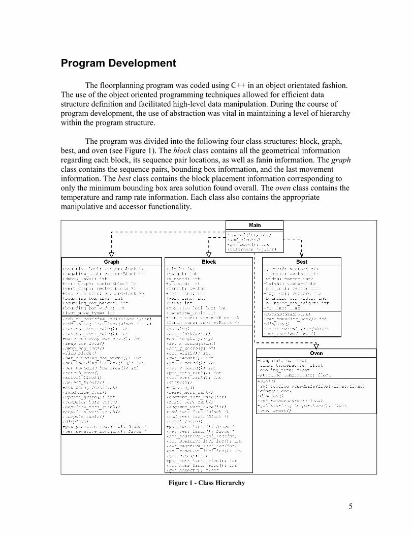
The program was divided into the following four class structures: block, graph,

best, and oven (see Figure 1). The block class contains all the geometrical information regarding each block, its sequence pair locations, as well as fanin information. The graph class contains the sequence pairs, bounding box information, and the last movement information. The best class contains the block placement information corresponding to only the minimum bounding box area solution found overall. The oven class contains the temperature and ramp rate information. Each class also contains the appropriate manipulative and accessor functionality.

Figure 1 - Class Hierarchy

6

Algorithm Discussion / Implementation Issues 1. Program Input / Output Characteristic

The input to the floorplanning program is a block description file (*.blk) which

contains the number of blocks and the dimensions of each one of the blocks. Following the layout optimization, the program is to output a layout description file (*.out). The layout description file consists of the bounding box width and height, the runtime, the sequence pairs, and the block (x,y) coordinate, width, and height information.

2. Graph Construction

2.1. Fanin Collection

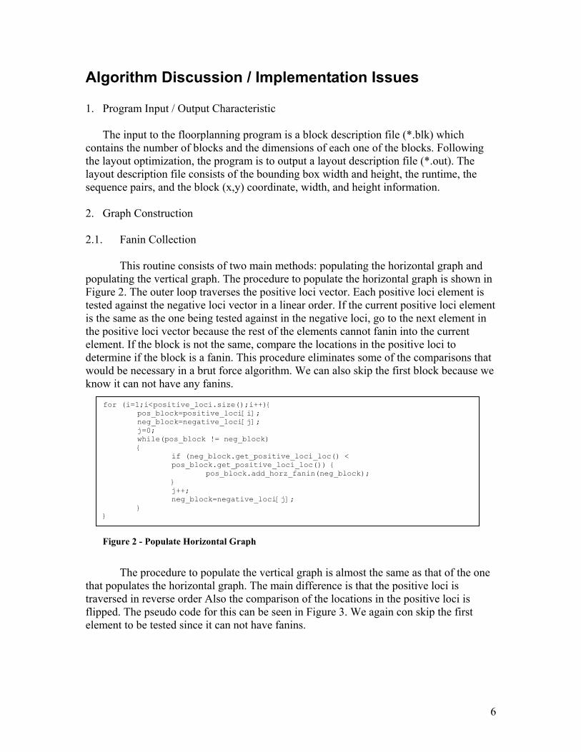
This routine consists of two main methods: populating the horizontal graph and populating the vertical graph. The procedure to populate the horizontal graph is shown in Figure 2. The outer loop traverses the positive loci vector. Each positive loci element is tested against the negative loci vector in a linear order. If the current positive loci element is the same as the one being tested against in the negative loci, go to the next element in the positive loci vector because the rest of the elements cannot fanin into the current element. If the block is not the same, compare the locations in the positive loci to determine if the block is a fanin. This procedure eliminates some of the comparisons that would be necessary in a brut force algorithm. We can also skip the first block because we know it can not have any fanins.

The procedure to populate the vertical graph is almost the same as that of the one that populates the horizontal graph. The main difference is that the positive loci is traversed in reverse order Also the comparison of the locations in the positive loci is flipped. The pseudo code for this can be seen in Figure 3. We again con skip the first element to be tested since it can not have fanins.

for (i=1;i<positive_loci.size();i++){ pos_block=positive_loci[i]; neg_block=negative_loci[j];

j=0; while(pos_block != neg_block)

{ if (neg_block.get_positive_loci_loc() < pos_block.get_positive_loci_loc()) {

pos_block.add_horz_fanin(neg_block); } j++; neg_block=negative_loci[j]; } }

Figure 2 - Populate Horizontal Graph

7

Figure 3 - Populate Vertical Graph

2.2. Topographical Sorting

The topographical sort routine implemented in the program is not really a topographical sort routine at all, at least in the classical sense. A typical topographical sort routine begins with a set of vertices and directed edges and essentially returns an ordering of vertices that has the property that the directed edges of each vertex are only directed toward vertices of higher order. Instead of doing this classical topographical sort (which is runtime expensive), the algorithm takes advantage of the fact that the sequence pair description of the graph reveals all the necessary information to compile a topographical sorted list based on the sequence pair information alone, without the extraneous compilation and sorting of corresponding edge information. The horizontal graph of blocks in topological order is found by sorting the sums of the indices of the positive and negative loci locations with respect to each block. Similarly, the vertical graph of blocks in topological order is found by sorting the differences of the indices of the positive and negative loci locations with respect to each block. This effective circumvention of traditional topographical sort methods results in significant runtime savings. 2.3. Longest Path Calculation

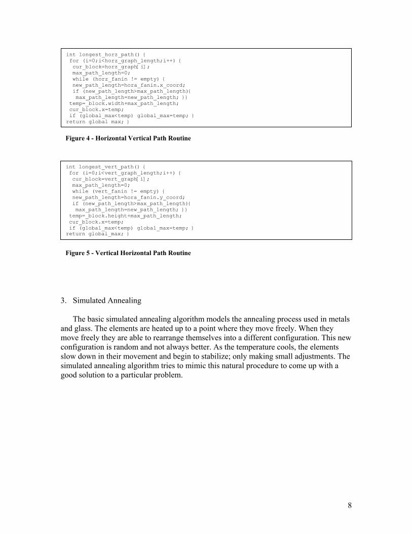
With the horizontal and vertical fanins for each block collected and the topographical ordering of the blocks known in both the horizontal and vertical directions, the longest horizontal and vertical path algorithms are very straightforward and mutually independent. In addition to calculating the longest paths, the algorithm also calculates the (x,y) coordinates of each block in the layout for the given sequence pair. The pseudo code for each of these routines is also given in Figure 4 and Figure 5.

for (i=positive_loci.size()-2;i>=0;i--){ pos_block=positive_loci[i];

neg_block=negative_loci[j]; while(pos_block.get_positive_loci_loc() != neg_block.get_positive_loci_loc() )

{ if (neg_block.get_positive_loci_loc() >

pos_block.get_positive_loci_loc()) {

pos_block.add_vert_fanin(neg_block); } j++; neg_block=negative_loci[j]; } j=0; }

8

3. Simulated Annealing

The basic simulated annealing algorithm models the annealing process used in metals and glass. The elements are heated up to a point where they move freely. When they move freely they are able to rearrange themselves into a different configuration. This new configuration is random and not always better. As the temperature cools, the elements slow down in their movement and begin to stabilize; only making small adjustments. The simulated annealing algorithm tries to mimic this natural procedure to come up with a good solution to a particular problem.

Figure 4 - Horizontal Vertical Path Routine

int longest_vert_path() { for (i=0;i<vert_graph_length;i++) { cur_block=vert_graph[i]; max_path_length=0; while (vert_fanin != empty) { new_path_length=hora_fanin.y_coord; if (new_path_length>max_path_length){ max_path_length=new_path_length; }} temp=_block.height+max_path_length; cur_block.x=temp; if (global_max<temp) global_max=temp; } return global_max; }

int longest_horz_path() { for (i=0;i<horz_graph_length;i++) { cur_block=horz_graph[i]; max_path_length=0; while (horz_fanin != empty) { new_path_length=hora_fanin.x_coord; if (new_path_length>max_path_length){ max_path_length=new_path_length; }} temp=_block.width+max_path_length; cur_block.x=temp; if (global_max<temp) global_max=temp; } return global max; }

Figure 5 - Vertical Horizontal Path Routine

9

The simulated annealing algorithm can be broken into three main areas: choosing how many moves to make at a certain temperature, when to allow a non-advancing move, and when to stop the entire annealing process. The pseudo code for this process can be found in Figure 6. The outer loop determines how long the entire annealing process runs. The annealing process ends when the ratio of the number of rejected moves to the number of total moves for the previous temperature is greater the 95%, or the annealing process has reached its final cooling temperature. The next loop determines how many moves occur at a specific temperature. The temperature will be reduced when a specified number of non-advancing moves have been completed or the total number of moves at the temperature is greater then a set value. At each temperature level all moves that provide advances are allowed, and some non-advancing moves are allowed based on the current temperature and a random factor. This allows for uphill movement to escape local minima. 3.1. Movement Selection

There are three possible moves in the program: swap positive loci, swap negative loci, and rotate – each self-explanatory. The movement selection is such that the sequence pair swaps occur more often at higher temperatures and less often at lower

Figure 7 - Annealing Routine Void anneal(int k,int tempratio) {

int scorechange,MT=1,M,N,uphill,reject=0,test=0, bestscore=0,currscore=0,backup=0; bool done=0; N=num_of_blocks*k; bestscore=current_graph_area; while ( ((reject/MT) < 0.95) && (oven != done)){ MT=0; reject=0; uphill=0; while ( (uphill < N) && (MT < 2*N) ) { M=getmove(); switch (M) { case 1 : swap_pos_loci; break; case 2 : swap_neg_loci; break; case 3 : rotate; default: break; } MT++; currscore=new_bounding_box_area; scorechange=bestscore-currscore; if ((scorechange > 0) || ( rand < exp(scorechange/tempratio*currtemp) )) { if (scorechange <0) uphill++; if (bestscore > currscore) { bestscore = currscore; if (best_best > currscore){ backup graph; best_best=currscore; } } } else { g.revert_move(); reject++; } } oven cool; } }

Figure 6 - Simulated Annealing Algorithm

10

temperatures, vice-versa for rotation. Since positive and negative loci swaps are essentially the same “size” move, given that a sequence pair type move is chosen, there is a 50% probability of choosing either a positive or negative loci swap, regardless of temperature.

11

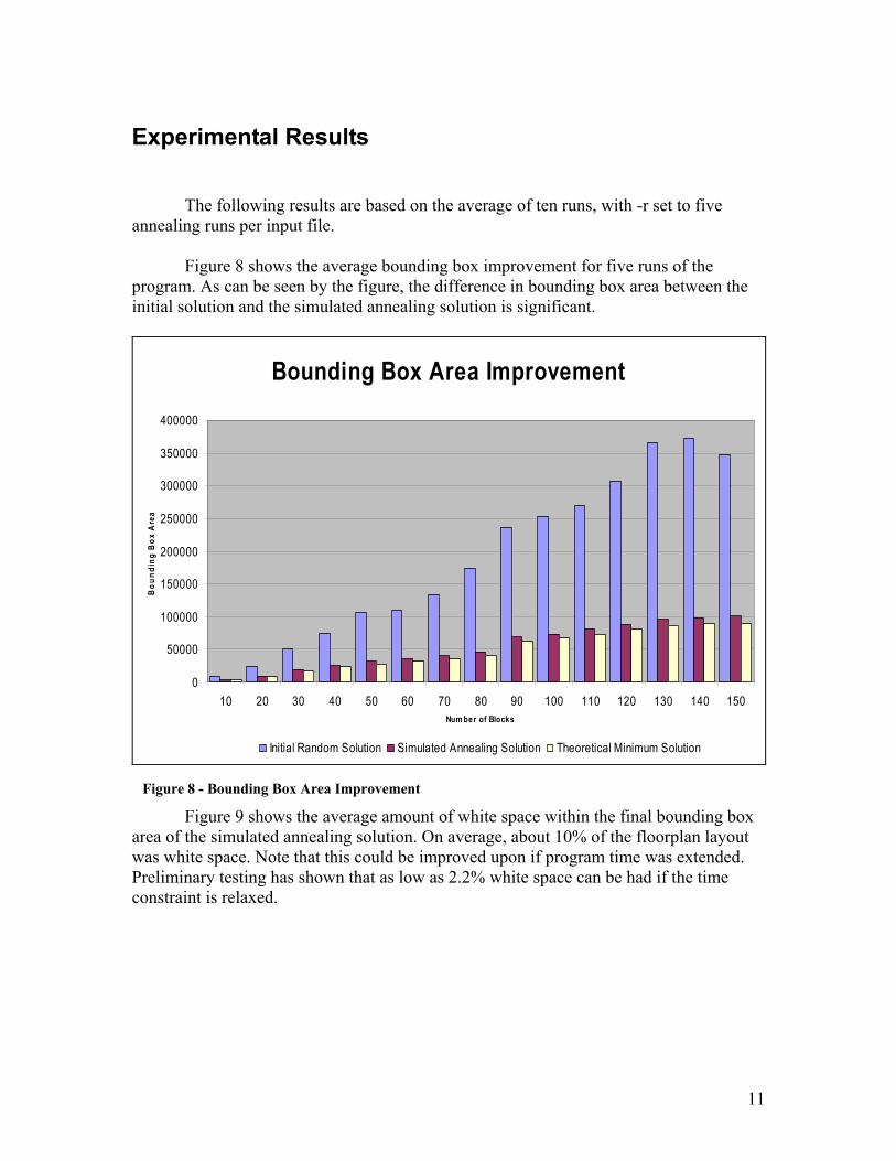
Experimental Results The following results are based on the average of ten runs, with -r set to five annealing runs per input file.

Figure 8 shows the average bounding box improvement for five runs of the program. As can be seen by the figure, the difference in bounding box area between the initial solution and the simulated annealing solution is significant.

Bounding Box Area Improvement

0

50000

100000

150000

200000

250000

300000

350000

400000

10 20 30 40 50 60 70 80 90 100 110 120 130 140 150Num ber of Blocks

Bou

ndin

g B

ox A

rea

Initial Random Solution Simulated Annealing Solution Theoretical Minimum Solution

Figure 9 shows the average amount of white space within the final bounding box area of the simulated annealing solution. On average, about 10% of the floorplan layout was white space. Note that this could be improved upon if program time was extended. Preliminary testing has shown that as low as 2.2% white space can be had if the time constraint is relaxed.

Figure 8 - Bounding Box Area Improvement

12

Percentage of White Space

0.00%

2.00%

4.00%

6.00%

8.00%

10.00%

12.00%

14.00%

10 20 30 40 50 60 70 80 90 100 110 120 130 140 150

Number of Blocks

Per

cent

Whi

te S

pace

Figure 9 - Percentage of White Space

Figure 10 shows the average amount of runtime required for program execution.

This is the average time required to produce the average percentage white space numbers in the previous figure.

Time

0

200

400

600

800

1000

1200

1400

1600

10 20 30 40 50 60 70 80 90 100 110 120 130 140 150

Number of Blocks

Tim

e

Figure 10 - Runtime Requirement

13

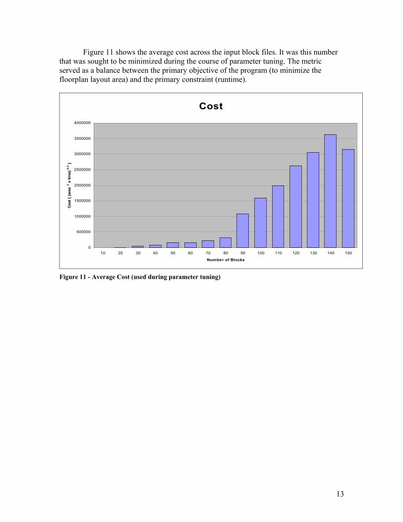
Figure 11 shows the average cost across the input block files. It was this number that was sought to be minimized during the course of parameter tuning. The metric served as a balance between the primary objective of the program (to minimize the floorplan layout area) and the primary constraint (runtime).

Cost

0

500000

1000000

1500000

2000000

2500000

3000000

3500000

4000000

10 20 30 40 50 60 70 80 90 100 110 120 130 140 150

Number of Blocks

Cost

{ (a

rea

2 x ti

me)

0.5 }

Figure 11 - Average Cost (used during parameter tuning)

14

Conclusions

Overall the project was very successful. Low floorplan layout areas were achieved in a fairly time efficient manner. For example, the runtimes for 10 and 20 block input files would take a fraction of a second, while 140 and 150 block input files would take at maximum around 20 minutes. An average 9-10% whitespace was encountered across the entire spectrum of block quantity input files. (Note: These numbers are for five runs of simulated annealing) The code itself, object orientated C++ class structures, is highly adaptable to future modifications. P.S. The longest path algorithm was updated since the data included in this report was taken. The average program runtime with the new version of this algorithm is only 95% of the original runtime.

15

Extensions To improve the runtime and thus allow the faster traversal of the solution space, several possible extensions to this work are listed as follows: Block Trip Distance: Take into account block area when swapping blocks in sequence pairs. Allow larger blocks to move less far than smaller blocks. Relate the relative distance a block with a certain area can move based on the current annealing temperature. Large Block “Sluggishness”: Allow larger blocks to be very mobile only at higher temperatures and reduce their mobility at lower temperatures. At low temperature, allow smaller blocks to move more readily than larger blocks. Low vs. High Aspect Ratio Rotations: Make the rotations of high aspect ratio block less likely and temperature dependent. Swap Near Blocks: By swapping blocks which are closely located, less fanin/fanout information is changed. In the ideal case, swapping adjacent blocks would result in do fanin/fanout recalculation. Longest Path Positive Short-Circuit: By rotating a block near the end of the topographical sorted list of blocks in either the horizontal or vertical directions, the new longest path (and thus new (x,y) coordinates) could be calculated from only that block onward. In the case where you were to swap two blocks, could start from the block earlier in the topographical sorted list of blocks in either the horizontal or vertical directions and proceed forward. This would be useful in cases where the block(s) occurred in the latter portions of the sequence pairs. Longest Path Negative Short-Circuit: By rotating a block near the beginning of the topographical sorted list of blocks in either the horizontal or vertical directions, the new longest path (and thus new (x,y) coordinates) could be calculated from only that block backward. In the case where you were to swap two blocks, could start from the block later in the topographical sorted list of blocks in either the horizontal or vertical directions. This would be useful in cases where the block(s) occurred in the earlier portions of the sequence pairs. Note that the origins would undergo a shift and have to be shifted back to the origin once at the end of the algorithm. Within Window Swaps: Implement a moving, variable-size window which would move across the floorplan layout. The move selection routine would only be allowed to select blocks from within the window to swap or rotate. The window size and movement rate would be temperature dependent. Temperature staging: Investigate the use of multiple temperature ramp stages.

16

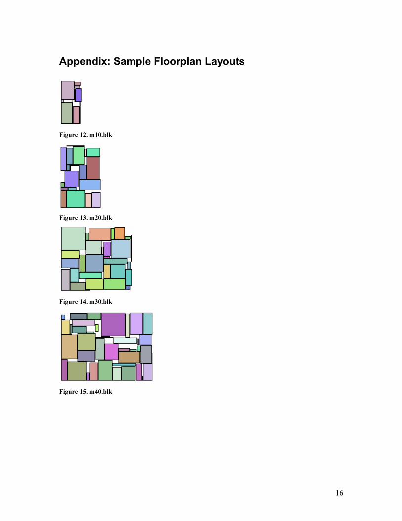
Appendix: Sample Floorplan Layouts

Figure 12. m10.blk

Figure 13. m20.blk

Figure 14. m30.blk

Figure 15. m40.blk

17

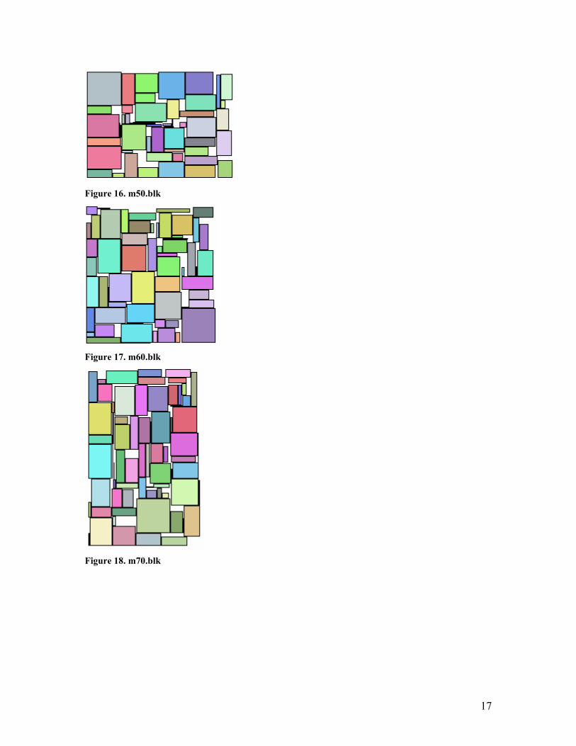
Figure 16. m50.blk

Figure 17. m60.blk

Figure 18. m70.blk

18

Figure 19. m80.blk

Figure 20. m90.blk

Figure 21. m100.blk

19

Figure 22. m110.blk

Figure 23. m120.blk

20

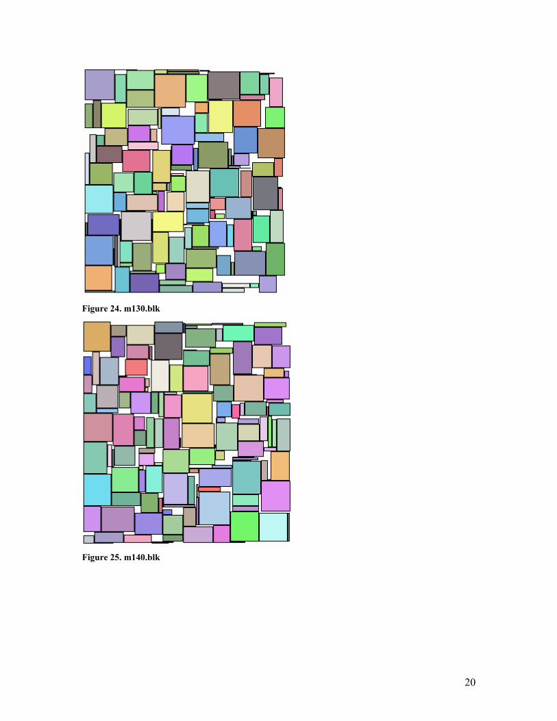
Figure 24. m130.blk

Figure 25. m140.blk

21

Figure 26. m150.blk

Figure 27. m10.blk w/ ~ 2% white space

Figure 28. m20.blk best w/ ~ 4% white space

Figure 29. m40.blk best w/ ~ 6% white space

[Disclaimer: No doglegs were abused during the compilation of this report.]