Geophysical Journal Internationaltopex.ucsd.edu/sandwell/publications/142.pdf · 2014-01-20 ·...
21
Geophysical Journal International Geophys. J. Int. (2014) doi: 10.1093/gji/ggt469 GJI Gravity, geodesy and tides Retracking CryoSat-2, Envisat and Jason-1 radar altimetry waveforms for improved gravity field recovery Emmanuel S. Garcia, 1 David T. Sandwell 1 and Walter H.F. Smith 2 1 Scripps Institution of Oceanography, University of California, San Diego, La Jolla, CA 92093-0225, USA. E-mail: [email protected] 2 National Oceanic and Atmospheric Administration, College Park, MD 20740, USA Accepted 2013 November 19. Received 2013 November 15; in original form 2013 February 13 SUMMARY Improving the accuracy of the marine gravity field requires both improved altimeter range precision and dense track coverage. After a hiatus of more than 15 yr, a wealth of suitable data is now available from the CryoSat-2, Envisat and Jason-1 satellites. The range precision of these data is significantly improved with respect to the conventional techniques used in operational oceanography by retracking the altimeter waveforms using an algorithm that is optimized for the recovery of the short-wavelength geodetic signal. We caution that this new approach, which provides optimal range precision, may introduce large-scale errors that would be unacceptable for other applications. In addition, CryoSat-2 has a new synthetic aperture radar (SAR) mode that should result in higher range precision. For this new mode we derived a simple, but approximate, analytic model for the shape of the SAR waveform that could be used in an iterative least-squares algorithm for estimating range. For the conventional waveforms, we demonstrate that a two-step retracking algorithm that was originally designed for data from prior missions (ERS-1 and Geosat) also improves precision on all three of the new satellites by about a factor of 1.5. The improved range precision and dense coverage from CryoSat-2, Envisat and Jason-1 should lead to a significant increase in the accuracy of the marine gravity field. Key words: Satellite geodesy; Gravity anomalies and Earth structure; Submarine tectonics and volcanism. INTRODUCTION The remote ocean basins remain largely unexplored by ships (Wessel & Chandler 2011) and are opaque to direct electromagnetic sounding, and so satellite radar altimeters are the tool of choice for global reconnaissance of the bathymetry and tectonics of the ocean basins (Smith 1998). Seafloor topography and crustal geology are isostatically compensated (Watts 2001) and so generate gravity anomalies primarily at wavelengths of ∼160 km and shorter (Smith & Sandwell 1994). Anomalies of horizontal wavelength λ are reduced in amplitude by an amount exp (-2π z /λ) when observed at a height z above the field’s source (Parker 1973), so the gravity signal of seafloor structure is insensible by gravity satellite missions such as GOCE (z ∼ 250 km) or GRACE (z ∼ 450 km). Radar altimeters sense the gravity field at the ocean surface so for a typical ocean depth of 4 km, the smallest spatial scale recoverable is ∼6 km. The scientific rationale for improved gravity is fairly mature and a set of papers related to this topic was published in a special issue of Oceanography (Smith 2004), entitled Bathymetry from Space. These studies show that achieving an accuracy of 1 mGal at a horizontal resolution of 6 km would enable major advances for a large number of basic science and practical applications. Radar altimeters measure the height of the ocean surface, which to a first approximation is a measure of gravitational potential. Gravity anomalies are the vertical derivative of the potential and they can be recovered from the two horizontal derivatives of the potential (i.e. sea surface gradient) through Laplace’s equation; 1 mGal of gravity anomaly roughly corresponds to 1 μrad (microradian) μrad of ocean surface slope. Therefore, achieving this 1 mGal threshold requires a radar altimeter range having a precision of 6 mm over 6-km horizontal distance. This precision could be derived from a single profile or a stack of repeated profiles. The gravity signal is most accurately recovered by working with along-track sea surface slopes rather than heights (Sandwell 1984; Olgiati et al. 1995). Many factors that affect the absolute height accuracy of altimetric sea level (Chelton et al. 2001) have correlation scales long enough that they yield negligible error in along-track slope (Sandwell & Smith 2009, table 3). The error budget for gravity recovery from altimetry is dominated by the range precision of the radar measurement. This precision can be improved by a process known as ‘retracking’ (Sandwell & Smith 2005, 2009). C The Authors 2014. Published by Oxford University Press on behalf of The Royal Astronomical Society. 1 Geophysical Journal International Advance Access published January 2, 2014 at University of California, San Diego on January 20, 2014 http://gji.oxfordjournals.org/ Downloaded from
Transcript of Geophysical Journal Internationaltopex.ucsd.edu/sandwell/publications/142.pdf · 2014-01-20 ·...

Geophysical Journal InternationalGeophys. J. Int. (2014) doi: 10.1093/gji/ggt469
GJI
Gra
vity
,ge
odes
yan
dtide
s
Retracking CryoSat-2, Envisat and Jason-1 radar altimetrywaveforms for improved gravity field recovery
Emmanuel S. Garcia,1 David T. Sandwell1 and Walter H.F. Smith2
1Scripps Institution of Oceanography, University of California, San Diego, La Jolla, CA 92093-0225, USA. E-mail: [email protected] Oceanic and Atmospheric Administration, College Park, MD 20740, USA
Accepted 2013 November 19. Received 2013 November 15; in original form 2013 February 13
S U M M A R YImproving the accuracy of the marine gravity field requires both improved altimeter rangeprecision and dense track coverage. After a hiatus of more than 15 yr, a wealth of suitabledata is now available from the CryoSat-2, Envisat and Jason-1 satellites. The range precisionof these data is significantly improved with respect to the conventional techniques used inoperational oceanography by retracking the altimeter waveforms using an algorithm that isoptimized for the recovery of the short-wavelength geodetic signal. We caution that this newapproach, which provides optimal range precision, may introduce large-scale errors that wouldbe unacceptable for other applications. In addition, CryoSat-2 has a new synthetic apertureradar (SAR) mode that should result in higher range precision. For this new mode we derived asimple, but approximate, analytic model for the shape of the SAR waveform that could be usedin an iterative least-squares algorithm for estimating range. For the conventional waveforms,we demonstrate that a two-step retracking algorithm that was originally designed for data fromprior missions (ERS-1 and Geosat) also improves precision on all three of the new satellitesby about a factor of 1.5. The improved range precision and dense coverage from CryoSat-2,Envisat and Jason-1 should lead to a significant increase in the accuracy of the marine gravityfield.
Key words: Satellite geodesy; Gravity anomalies and Earth structure; Submarine tectonicsand volcanism.
I N T RO D U C T I O N
The remote ocean basins remain largely unexplored by ships (Wessel & Chandler 2011) and are opaque to direct electromagnetic sounding,and so satellite radar altimeters are the tool of choice for global reconnaissance of the bathymetry and tectonics of the ocean basins (Smith1998). Seafloor topography and crustal geology are isostatically compensated (Watts 2001) and so generate gravity anomalies primarily atwavelengths of !160 km and shorter (Smith & Sandwell 1994). Anomalies of horizontal wavelength ! are reduced in amplitude by an amountexp ("2" z/!) when observed at a height z above the field’s source (Parker 1973), so the gravity signal of seafloor structure is insensible bygravity satellite missions such as GOCE (z ! 250 km) or GRACE (z ! 450 km). Radar altimeters sense the gravity field at the ocean surfaceso for a typical ocean depth of 4 km, the smallest spatial scale recoverable is !6 km. The scientific rationale for improved gravity is fairlymature and a set of papers related to this topic was published in a special issue of Oceanography (Smith 2004), entitled Bathymetry fromSpace. These studies show that achieving an accuracy of 1 mGal at a horizontal resolution of 6 km would enable major advances for a largenumber of basic science and practical applications.
Radar altimeters measure the height of the ocean surface, which to a first approximation is a measure of gravitational potential. Gravityanomalies are the vertical derivative of the potential and they can be recovered from the two horizontal derivatives of the potential (i.e.sea surface gradient) through Laplace’s equation; 1 mGal of gravity anomaly roughly corresponds to 1 µrad (microradian) µrad of oceansurface slope. Therefore, achieving this 1 mGal threshold requires a radar altimeter range having a precision of 6 mm over 6-km horizontaldistance. This precision could be derived from a single profile or a stack of repeated profiles. The gravity signal is most accurately recoveredby working with along-track sea surface slopes rather than heights (Sandwell 1984; Olgiati et al. 1995). Many factors that affect the absoluteheight accuracy of altimetric sea level (Chelton et al. 2001) have correlation scales long enough that they yield negligible error in along-trackslope (Sandwell & Smith 2009, table 3). The error budget for gravity recovery from altimetry is dominated by the range precision of the radarmeasurement. This precision can be improved by a process known as ‘retracking’ (Sandwell & Smith 2005, 2009).
C# The Authors 2014. Published by Oxford University Press on behalf of The Royal Astronomical Society. 1
Geophysical Journal International Advance Access published January 2, 2014
at University of California, San D
iego on January 20, 2014http://gji.oxfordjournals.org/
Dow
nloaded from
2 E.S. Garcia, D.T. Sandwell and W.H.F. Smith
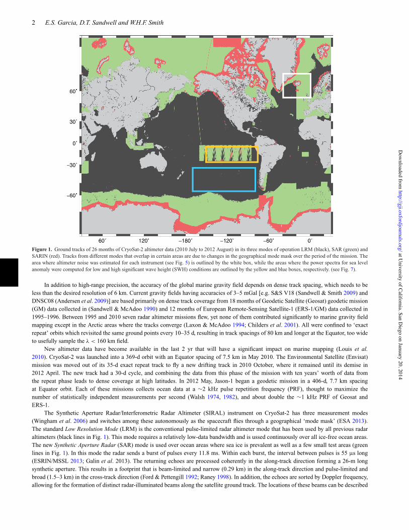
Figure 1. Ground tracks of 26 months of CryoSat-2 altimeter data (2010 July to 2012 August) in its three modes of operation LRM (black), SAR (green) andSARIN (red). Tracks from different modes that overlap in certain areas are due to changes in the geographical mode mask over the period of the mission. Thearea where altimeter noise was estimated for each instrument (see Fig. 5) is outlined by the white box, while the areas where the power spectra for sea levelanomaly were computed for low and high significant wave height (SWH) conditions are outlined by the yellow and blue boxes, respectively. (see Fig. 7).
In addition to high-range precision, the accuracy of the global marine gravity field depends on dense track spacing, which needs to beless than the desired resolution of 6 km. Current gravity fields having accuracies of 3–5 mGal [e.g. S&S V18 (Sandwell & Smith 2009) andDNSC08 (Andersen et al. 2009)] are based primarily on dense track coverage from 18 months of Geodetic Satellite (Geosat) geodetic mission(GM) data collected in (Sandwell & McAdoo 1990) and 12 months of European Remote-Sensing Satellite-1 (ERS-1/GM) data collected in1995–1996. Between 1995 and 2010 seven radar altimeter missions flew, yet none of them contributed significantly to marine gravity fieldmapping except in the Arctic areas where the tracks converge (Laxon & McAdoo 1994; Childers et al. 2001). All were confined to ‘exactrepeat’ orbits which revisited the same ground points every 10–35 d, resulting in track spacings of 80 km and longer at the Equator, too wideto usefully sample the ! < 160 km field.
New altimeter data have become available in the last 2 yr that will have a significant impact on marine mapping (Louis et al.2010). CryoSat-2 was launched into a 369-d orbit with an Equator spacing of 7.5 km in May 2010. The Environmental Satellite (Envisat)mission was moved out of its 35-d exact repeat track to fly a new drifting track in 2010 October, where it remained until its demise in2012 April. The new track had a 30-d cycle, and combining the data from this phase of the mission with ten years’ worth of data fromthe repeat phase leads to dense coverage at high latitudes. In 2012 May, Jason-1 began a geodetic mission in a 406-d, 7.7 km spacingat Equator orbit. Each of these missions collects ocean data at a !2 kHz pulse repetition frequency (PRF), thought to maximize thenumber of statistically independent measurements per second (Walsh 1974, 1982), and about double the !1 kHz PRF of Geosat andERS-1.
The Synthetic Aperture Radar/Interferometric Radar Altimeter (SIRAL) instrument on CryoSat-2 has three measurement modes(Wingham et al. 2006) and switches among these autonomously as the spacecraft flies through a geographical ‘mode mask’ (ESA 2013).The standard Low Resolution Mode (LRM) is the conventional pulse-limited radar altimeter mode that has been used by all previous radaraltimeters (black lines in Fig. 1). This mode requires a relatively low-data bandwidth and is ussed continuously over all ice-free ocean areas.The new Synthetic Aperture Radar (SAR) mode is used over ocean areas where sea ice is prevalent as well as a few small test areas (greenlines in Fig. 1). In this mode the radar sends a burst of pulses every 11.8 ms. Within each burst, the interval between pulses is 55 µs long(ESRIN/MSSL 2013; Galin et al. 2013). The returning echoes are processed coherently in the along-track direction forming a 26-m longsynthetic aperture. This results in a footprint that is beam-limited and narrow (0.29 km) in the along-track direction and pulse-limited andbroad (1.5–3 km) in the cross-track direction (Ford & Pettengill 1992; Raney 1998). In addition, the echoes are sorted by Doppler frequency,allowing for the formation of distinct radar-illuminated beams along the satellite ground track. The locations of these beams can be described
at University of California, San D
iego on January 20, 2014http://gji.oxfordjournals.org/
Dow
nloaded from
Retracking altimetry for gravity recovery 3
by a ‘look’ angle measured with respect to nadir. The return signals from multiple beams can be combined after performing range migration(Wingham et al. 2004), in a process termed ‘multilooking’, or ‘multilook averaging’. There is a third mode of operation to measure elevationand cross-track slope over land ice surfaces where there is significant topographic slope (red lines in Fig. 1). This SAR/Interferometric RadarAltimeter (SARIN) mode utilizes the two antennas on CryoSat-2 to form a cross-track interferometer. The echoes received by each antennaundergo Doppler beam processing as in SAR mode, but the number of waveforms averaged is lower due to the longer interval between burstsof 47.17 ms for SARIN mode. Both the SAR and SARIN modes require a very high bandwidth data link to the ground stations. CryoSat-2’sSAR and SARIN modes were designed for measurements of sea ice and grounded ice, respectively (Wingham et al. 2006), but some data inthese modes have been collected over ocean areas (Giles et al. 2012; Galin et al. 2013) for experiments which range from the observationof mesoscale sea surface variability (Dibarboure et al. 2011) to the recovery of the short-wavelength gravity signal (Stenseng & Andersen2012), with the latter being the main focus of the present paper. If all else were equal, SAR-mode altimetry should be about two times moreprecise than conventional altimetry (Jensen & Raney 1998). However, CryoSat-2’s implementation, in which the echoes from one burst arereceived before the next burst is transmitted, means that the instrument makes measurements only !30 per cent of the available time, whichis suboptimal (Raney 2011). Thus, the performance gain, if any, of CryoSat-2’s SAR and SARIN over its LRM, needs to be studied.
This paper addresses the following questions: (1) could the range measurements of these new altimeters be improved by the two-step retracking method Sandwell & Smith (2005) developed for ERS-1? (2) Could this method, which was developed for conventional‘pulse-limited’ altimetry, be adapted to the CryoSat-2 SAR and SARIN cases where the radar waveform is both pulse-limited and alsoDoppler-beam-limited? (3) When the method is applied to conventional waveforms acquired by averaging 2-kHz PRF echoes, how do theresults compare with previous results obtained from the 1-kHz PRF instruments Geosat and ERS-1? (4) How do the CryoSat-2 SAR andSARIN results compare with those of the CryoSat-2 LRM and other conventional altimeters? (5) How does two-step retracking affect thespectral properties of the range measurements for the newer altimeters? This analysis would determine how well our techniques recover thevarious spatial scales that are present in the range signal.
As described above, we are only concerned with recovering the along-track ocean surface slope by estimating the range from consecutiveradar altimeter waveforms. Therefore, our waveform model is less complex than is required for applications where absolute ocean surfaceheight is needed. For example, we can neglect the effects of earth curvature, slow changes in antenna mispointing, and can use a Gaussianapproximation for the point target response. We make these approximations for developing a simplified version of the analytical ‘Brown’model for a conventional altimeter (Brown 1977; Rodrıguez 1988; Amarouche et al. 2004). Then, using the same approximations, we developan analytic formula for the shape of the SAR waveforms under the ideal condition of small radar mispointing angle. Analyticity is a virtuebecause it allows one to obtain the partial derivatives of least-squares model misfit with respect to model parameters, facilitating the searchfor a best-fit model by Gauss–Newton iterative steps. We evaluate the deficiencies of the analytical model through a comparison with amore fully developed waveform model (SAMOSA Project, Salvatore Dinardo 2012, personal communication) that also includes the effectsof multilooking and radar mispointing (Wingham et al. 2004; Cotton et al. 2010). In addition, we show good agreement between our SARretracking sea surface slope results and the slope derived from an independent analysis of the same data (Labroue et al. 2012).
Next, we show the results from least squares analysis of our waveform models applied to data from the different CryoSat-2 modes. Then,in order to assess the range precision of CryoSat-2, Envisat, and Jason-1 compared to ERS-1 and Geosat, we gathered all the data available forregions containing acquisitions from each of the CryoSat-2 modes. We quantified range precision by computing statistics on the range valuesproduced by our retracking algorithms. In addition, we computed power spectral densities of the derived quantities such as sea level anomalyand significant wave height. Throughout these analyses, we compare the results obtained for data with and without two-step retracking. Thisallows us to discuss the benefits of applying this method in reducing the noise levels in range. Finally, we put our findings in context byexamining the issue of correlated model errors during waveform retracking. The insights we have gained in this study have implications forunderstanding the contributions of each altimeter data set to the modelling of the global gravity field, which will be the focus of future work.
WAV E F O R M M O D E L S
A satellite altimeter senses the range to the sea surface by emitting a series of frequency-modulated chirp signals designed to act like briefradar pulses. These then interact with the ocean surface, and the received power of the reflected signal is recorded by the satellite altimeter overa short observation window, spanning 400 ns of travel time, equivalent to 60 m of range. Averages of the power received from many echoesare referred to as altimeter waveforms, and their shape may be described mathematically using a multiparameter model that is a function ofthe time elapsed since the signal transmission. The expected round-trip time varies by order 100 µs as the satellite moves around its orbit, andso the instrument employs a target tracking scheme to keep the sea surface echoes aligned within the observation window. Fitting a parametricmodel to the waveform is crucial to improving the estimate of range beyond what was estimated by the on-board tracker, and this parametricmodelling is called ‘retracking’.
The shape of the return radar waveforms collected by the altimeter can be described as a function of the delay time # , which is thesampling time t referenced to the arrival time of the waveform t0, such that # = t " t0. The power versus delay time for the model radar returnpulse M (# ) is given by the triple convolution of the point target response P (# ), the effective area of the ocean illuminated versus time S (# ),and the ocean surface roughness function G (# ) (Brown 1977; Hayne 1980; MacArthur et al. 1987; Hayne et al. 1994; Rodriguez & Martin1994; Chelton et al. 2001; Amarouche et al. 2004).
M (# ) = P (# ) $ S (# ) $ G (# ) . (1)
at University of California, San D
iego on January 20, 2014http://gji.oxfordjournals.org/
Dow
nloaded from
4 E.S. Garcia, D.T. Sandwell and W.H.F. Smith
The source time function has the form p0[sin("#/#p)/("#/#p)]2 because the pulse is formed by deconvolution of a frequency modulatedchirp, and p0 is the peak power of the pulse. The bandwidth of the chirp is 320 MHz. This results in an effective pulse length, # p, of 3.125ns, for an effective range resolution of the radar of 0.467 m. To simplify the convolution integrals, it is customary to approximate the sourcetime function with a Gaussian function of the form
P (# ) = p0 exp
!"# 2
2$ 2p
"
, (2)
where $p is the standard deviation of the Gaussian function that models the point target response, and is related to the effective pulse lengthby $p = 0.513#p (Amarouche et al. 2004). This approximation leads to a range bias of about 1 cm and could be corrected using a lookuptable (Thibaut et al. 2010). We do not apply this correction because the slope of this correction will be much less than 1 µrad. The roughnessof the ocean surface due to ocean waves is also well approximated by a Gaussian function (Stewart 1985)
G (# ) = 2
$hc%
2"exp
#"# 2
2$ 2h
$, (3)
where $h is related to the significant wave height hswh by
$h = hswh
2c, (4)
where c is the speed of light. The order of the triple convolution given in eq. (1) is unimportant so we begin by convolving the Gaussianapproximation to the source function with the Gaussian wave height distribution resulting in
P (# ) $ G (# ) = PG (# ) = 2p0
$c%
2"exp
#"# 2
2$ 2
$, (5)
where $ 2 = $ 2h + $ 2
p .We note that for the purpose of recovering gravity from sea surface slopes the absolute scaling of eq. (5) is arbitrary, as we do not seek to
recover calibrated values of the radar backscatter. The final convolution of the Gaussian pulse with the effective area of the ocean illuminatedby the radar determines the shape of the model waveform.
The treatment that we present below to obtain the flat surface response S (# ) is meant to illustrate that the difference between thepulse-limited and SAR mode waveform models originates from the contrast in the geometries of the areas effectively illuminated by the radarpulse on the sea surface. To facilitate this, we will make the assumption that the diameter of the pulse-limited footprint is much less than thediameter of the antenna beam pattern so the variation in antenna power within the pulse-limited area is small and can be approximated as aconstant. This approximation will break down when the off-nadir pointing angle reaches a large fraction of the antenna beam angle. However,multiplying an ad hoc exponential decay function to the effective illuminated area results in the same functional form as a derivation of the flatsurface response that takes into account the finite width of the radar antenna gain pattern, up to within a multiplicative factor (Appendix A).Since we are most interested in measuring the arrival time of the return pulse, our analysis is not concerned with the amplitude of the pulseand thus our methods are sufficient for the sole purpose of measuring sea surface slopes.
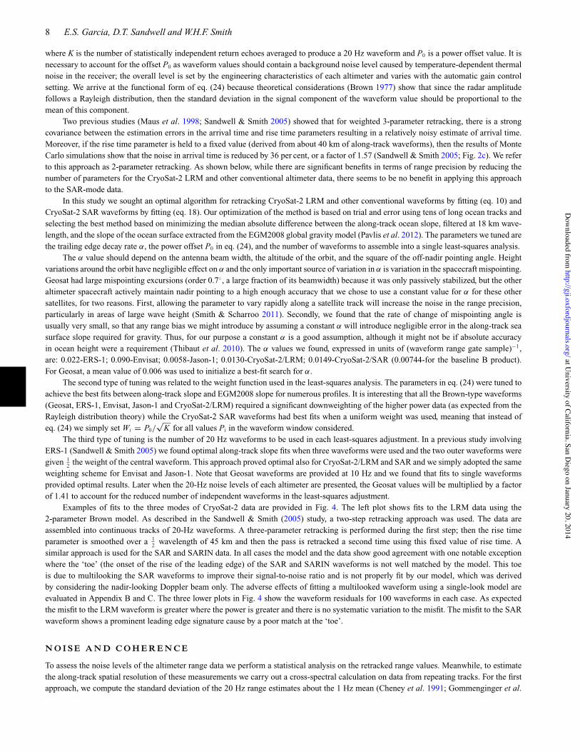
S I M P L I F I E D B ROW N M O D E L
Over the ocean the CryoSat-2 altimeter is operated in two modes (Fig. 2). The SIRAL antenna is slightly elliptical, but for LRM we considerthe pulses as having approximately spherical wave fronts. The wave front reflects from an annulus on the ocean surface having an areaA(r ) = 2"rdr, where r is the radius of the annulus and dr is the width of the annulus. The approximate radius of the annulus versus time isgiven by (Walsh et al. 1978; Hayne 1980; Stewart 1985)
r (# ) !=#
hc#%
$1/2
(6)
in which h is the altitude of the radar antenna above the surface, and c is the propagation speed of the radar pulse. The factor % = 1 + h/Raccounts for the curvature of the Earth, R (Rodrıguez 1988; Chelton et al. 1989). While the radius of the annulus increases as the square rootof time, the thickness of the annulus per unit time decreases as the square root of time. This can be seen by approximating the thickness ofthe annulus dr by the rate of growth of the radius of the encircling ring,
drd#
!=12
#hc%#
$1/2
(7)
and so therefore the area of the annulus as a function of # is uniform after the arrival of the pulse:
S (# ) = ("hc/%) H (# ) . (8)
at University of California, San D
iego on January 20, 2014http://gji.oxfordjournals.org/
Dow
nloaded from

Retracking altimetry for gravity recovery 5
Figure 2. Interaction of a radar pulse with a flat surface. Area illuminated in standard LRM mode after the arrival of the pulse (left-hand side). Area illuminatedby the synthetic aperture radar (SAR) method where w is the effective width of the focused beam in the along-track direction (right-hand side).
The final step in generating the model waveform is to convolve the effective area versus time with the Gaussian pulse function
M (# ) = P (# ) $ G (# ) $ S (# ) = hc$%
%2" p0
% &
"&exp
!" (# " # ')2
2$ 2
"
H&# '' d# '. (9)
Integrating (9) using formula 7.4.2 in Abramowitz & Stegun (1964) results in the familiar ‘Brown model’ (Brown 1977) waveformmodel
M (# ) = hc"p0
%2
%[1 + er f (&)] exp ("'# ) = A
2
(1 + er f
##%2$
$)exp ("'# ) , (10)
where A is a scaling factor similar to a peak amplitude and & = #/%
2$ . The exponential decay accounts for the antenna’s gain pattern underthe assumption that the line of maximum antenna gain makes an angle with nadir (the ‘mispointing’ angle) which is small compared to theantenna’s beam width (Rodrıguez 1988; Amarouche et al. 2004). Also assumed in (10) is that the antenna gain pattern is circular. This iscorrect for all altimeter satellites except CryoSat-2, which has a slightly elliptical antenna pattern; however, CryoSat-2 conventional modewaveforms can be adequately approximated by assuming a circular pattern having a beam width squared equal to the harmonic mean ofCryoSat-2’s actual major and minor beam widths squared (Wingham & Wallis 2010; Smith & Scharroo 2011; Smith et al. 2011).
The partial derivatives of the model with respect to t0, $ , and A are approximately
( M(t0
= "A
$%
2"e"&2
, (11)
at University of California, San D
iego on January 20, 2014http://gji.oxfordjournals.org/
Dow
nloaded from

6 E.S. Garcia, D.T. Sandwell and W.H.F. Smith
Figure 3. Brown model waveform including the exponential approximation to the trailing edge decay for a 2 m SWH (upper). Model derivatives with respectto arrival time (dashed) and rise time (dotted) are also shown. SAR model waveform for a 2 m SWH and including the exponential decay of the trailing edgeapproximating the antenna gain effect. Model derivatives are also shown (lower).
( M($
= "A$%
"&e"&2
(12)
( M( A
= MA
, (13)
respectively. Note that to simplify these expressions and the least squares analysis we have assumed that the slope of the exponential decaywith respect to time is smaller than the more important leading terms. Plots of this simplified Brown model and its partial derivatives areprovided in Fig. 3 (upper).
A P P ROX I M AT E S A R M O D E L
A similar approach is used to develop the waveform shape for the SAR model as well as its derivatives with respect to the model parameters.When CryoSat-2 operates in its SAR mode, the PRF is high enough to allow Doppler beam sharpening. Processing a group of 64 echoesyields 64 Doppler beams, fanned out in the direction of flight (Raney 1998). One of these beams looks at nadir while the others look fore andaft; each subtends a width w along the ground. By selecting data from a particular beam, one may select slices through the annulus sampledby the radar pulse (Fig. 2b). Here, we will develop a simple expression approximating the mean power expected from only the nadir-lookingbeam having an effective width w in the along-track direction (Raney 1998; Wingham et al. 2004). An assessment of the effects of using anadir-only beam model to fit a multilooked waveform with small off-nadir pointing angle is provided in Appendices B and C. In this case thearea of the illuminated ocean surface is approximately given by
S (# ) != 2wdrd#
H (# ), (14)
when w ( r (Fig. 2), implying that the illuminated beam pattern can be treated as close to rectangular. So by again invoking (eq. 7), the areaversus delay time function is given by
S (# ) = w
#hc%#
$1/2
H (# ) . (15)
at University of California, San D
iego on January 20, 2014http://gji.oxfordjournals.org/
Dow
nloaded from

Retracking altimetry for gravity recovery 7
The model return waveform is the convolution of the Gaussian pulse with this area versus time function
M (# ) = P (# ) $ G (# ) $ S (# ) = wp0
$
*2hc%"
% &
"&exp
!" (# " # ')2
2$ 2
"
# '"1/2 H&# '' d# '. (16)
This integration, including an approximation to the CryoSat-2 antenna beam pattern, is provided in Appendix A. The final result is
M (# ) = A$"1/2 exp+" #
4$ 2
,D"1/2
#"#
$
$exp ("'# ) , (17)
where D)(z) is the parabolic cylinder function of order ) and argument z.As in the case of the Brown model, we would like to compute the partial derivatives of the model with respect to t0, $ and A. The details
are provided in Appendix A, but we summarize the results here:
M = A$"1/2 exp#
"14
z2
$D"1/2 (z) exp ("'# ) , (18)
( M(t0
= "A$"3/2 exp#
"14
z2
$D1/2 (z) , (19)
( M($
= "A$"3/2 exp#
"14
z2
$ (12
D"1/2 (z) " zD1/2 (z))
, (20)
( M( A
= MA
, (21)
where z = "#/$ . As in the case of the Brown model we simplify these expressions by assuming that the slope of the exponential decay withrespect to time is smaller than the more important leading terms. Plots of this SAR model and its derivatives are provided in Fig. 3 (lower).
L E A S T S Q UA R E S A NA LY S I S
The standard approach in operational oceanography is to retrack the waveforms of conventional altimeters by fitting a mathematical model asin eq. (10). One such technique has been referred to as MLE (Amarouche et al. 2004; Thibaut et al. 2010). If the retracker fits four unknownparameters A-amplitude, t0-arrival time, $ -rise time and '-trailing edge decay it is commonly called ‘MLE4’, while if the trailing edge decayparameter ' is held fixed, then it is called ‘MLE3’. In prior work (Sandwell & Smith 2005) and in this study, we use a least-squares approach,which we call 3-parameter retracking. For our algorithm, the criteria for convergence depends on the following misfit function:
* 2 =N-
i=1
#Pi " M(ti ; t0, $, A)
Wi
$2
, (22)
where the summation is over N waveform power samples. The waveform model M is evaluated for every ti, and a starting model is calculatedfrom some initial estimates A0, $ 0 and t0
0 for the fitting parameters. The best fitting model is found through successive iteration, and at eachiteration the differences between the new parameter values A j+1, $ j+1 and t j+1
0 and the current values Aj, $ j and t j0 are found by solving the
following linear system:.
///////////0
P1 " M j1
P2 " M j2
...
...
PN " M jN
1
222222222223
=
.
/////////0
( M(t1;t j0 ,$ j ,A j )(t0
( M(t1;t j0 ,$ j ,A j )($
( M(t1;t j0 ,$ j ,A j )( A
......
...
......
...
( M(tN ;t0,$,A)(t0
( M(t1;t j0 ,$ j ,A j )($
( M(t1;t j0 ,$ j ,A j )( A
1
2222222223
.
///0
t j+10 " t j
0
$ j+1 " $ j
A j+1 " A j
1
2223. (23)
In the case of non-uniform weights, (23) should be modified by dividing both sides of the ith equation by the weights Wi. The expressions forthe partial derivatives of the model with respect to the parameters are given by eqs (11)–(13) for the conventional pulse-limited waveform,and eqs (19)–(21) for the SAR mode waveform. The partial derivatives are then evaluated for the set of parameter values at each step j andat every gate i. The weights Wi in eq. (22) represent the uncertainty in the recorded waveform power, and for the conventional pulse-limitedwaveforms we use the functional form
Wi = (Pi + P0)%K
, (24)
at University of California, San D
iego on January 20, 2014http://gji.oxfordjournals.org/
Dow
nloaded from
8 E.S. Garcia, D.T. Sandwell and W.H.F. Smith
where K is the number of statistically independent return echoes averaged to produce a 20 Hz waveform and P0 is a power offset value. It isnecessary to account for the offset P0 as waveform values should contain a background noise level caused by temperature-dependent thermalnoise in the receiver; the overall level is set by the engineering characteristics of each altimeter and varies with the automatic gain controlsetting. We arrive at the functional form of eq. (24) because theoretical considerations (Brown 1977) show that since the radar amplitudefollows a Rayleigh distribution, then the standard deviation in the signal component of the waveform value should be proportional to themean of this component.
Two previous studies (Maus et al. 1998; Sandwell & Smith 2005) showed that for weighted 3-parameter retracking, there is a strongcovariance between the estimation errors in the arrival time and rise time parameters resulting in a relatively noisy estimate of arrival time.Moreover, if the rise time parameter is held to a fixed value (derived from about 40 km of along-track waveforms), then the results of MonteCarlo simulations show that the noise in arrival time is reduced by 36 per cent, or a factor of 1.57 (Sandwell & Smith 2005; Fig. 2c). We referto this approach as 2-parameter retracking. As shown below, while there are significant benefits in terms of range precision by reducing thenumber of parameters for the CryoSat-2 LRM and other conventional altimeter data, there seems to be no benefit in applying this approachto the SAR-mode data.
In this study we sought an optimal algorithm for retracking CryoSat-2 LRM and other conventional waveforms by fitting (eq. 10) andCryoSat-2 SAR waveforms by fitting (eq. 18). Our optimization of the method is based on trial and error using tens of long ocean tracks andselecting the best method based on minimizing the median absolute difference between the along-track ocean slope, filtered at 18 km wave-length, and the slope of the ocean surface extracted from the EGM2008 global gravity model (Pavlis et al. 2012). The parameters we tuned arethe trailing edge decay rate ', the power offset P0 in eq. (24), and the number of waveforms to assemble into a single least-squares analysis.
The ' value should depend on the antenna beam width, the altitude of the orbit, and the square of the off-nadir pointing angle. Heightvariations around the orbit have negligible effect on ' and the only important source of variation in ' is variation in the spacecraft mispointing.Geosat had large mispointing excursions (order 0.7), a large fraction of its beamwidth) because it was only passively stabilized, but the otheraltimeter spacecraft actively maintain nadir pointing to a high enough accuracy that we chose to use a constant value for ' for these othersatellites, for two reasons. First, allowing the parameter to vary rapidly along a satellite track will increase the noise in the range precision,particularly in areas of large wave height (Smith & Scharroo 2011). Secondly, we found that the rate of change of mispointing angle isusually very small, so that any range bias we might introduce by assuming a constant ' will introduce negligible error in the along-track seasurface slope required for gravity. Thus, for our purpose a constant ' is a good assumption, although it might not be if absolute accuracyin ocean height were a requirement (Thibaut et al. 2010). The ' values we found, expressed in units of (waveform range gate sample)"1,are: 0.022-ERS-1; 0.090-Envisat; 0.0058-Jason-1; 0.0130-CryoSat-2/LRM; 0.0149-CryoSat-2/SAR (0.00744-for the baseline B product).For Geosat, a mean value of 0.006 was used to initialize a best-fit search for '.
The second type of tuning was related to the weight function used in the least-squares analysis. The parameters in eq. (24) were tuned toachieve the best fits between along-track slope and EGM2008 slope for numerous profiles. It is interesting that all the Brown-type waveforms(Geosat, ERS-1, Envisat, Jason-1 and CryoSat-2/LRM) required a significant downweighting of the higher power data (as expected from theRayleigh distribution theory) while the CryoSat-2 SAR waveforms had best fits when a uniform weight was used, meaning that instead ofeq. (24) we simply set Wi = P0/
%K for all values Pi in the waveform window considered.
The third type of tuning is the number of 20 Hz waveforms to be used in each least-squares adjustment. In a previous study involvingERS-1 (Sandwell & Smith 2005) we found optimal along-track slope fits when three waveforms were used and the two outer waveforms weregiven 1
2 the weight of the central waveform. This approach proved optimal also for CryoSat-2/LRM and SAR and we simply adopted the sameweighting scheme for Envisat and Jason-1. Note that Geosat waveforms are provided at 10 Hz and we found that fits to single waveformsprovided optimal results. Later when the 20-Hz noise levels of each altimeter are presented, the Geosat values will be multiplied by a factorof 1.41 to account for the reduced number of independent waveforms in the least-squares adjustment.
Examples of fits to the three modes of CryoSat-2 data are provided in Fig. 4. The left plot shows fits to the LRM data using the2-parameter Brown model. As described in the Sandwell & Smith (2005) study, a two-step retracking approach was used. The data areassembled into continuous tracks of 20-Hz waveforms. A three-parameter retracking is performed during the first step; then the rise timeparameter is smoothed over a 1
2 wavelength of 45 km and then the pass is retracked a second time using this fixed value of rise time. Asimilar approach is used for the SAR and SARIN data. In all cases the model and the data show good agreement with one notable exceptionwhere the ‘toe’ (the onset of the rise of the leading edge) of the SAR and SARIN waveforms is not well matched by the model. This toeis due to multilooking the SAR waveforms to improve their signal-to-noise ratio and is not properly fit by our model, which was derivedby considering the nadir-looking Doppler beam only. The adverse effects of fitting a multilooked waveform using a single-look model areevaluated in Appendix B and C. The three lower plots in Fig. 4 show the waveform residuals for 100 waveforms in each case. As expectedthe misfit to the LRM waveform is greater where the power is greater and there is no systematic variation to the misfit. The misfit to the SARwaveform shows a prominent leading edge signature cause by a poor match at the ‘toe’.
N O I S E A N D C O H E R E N C E
To assess the noise levels of the altimeter range data we perform a statistical analysis on the retracked range values. Meanwhile, to estimatethe along-track spatial resolution of these measurements we carry out a cross-spectral calculation on data from repeating tracks. For the firstapproach, we compute the standard deviation of the 20 Hz range estimates about the 1 Hz mean (Cheney et al. 1991; Gommenginger et al.
at University of California, San D
iego on January 20, 2014http://gji.oxfordjournals.org/
Dow
nloaded from

Retracking altimetry for gravity recovery 9
Figure 4. Least-squares fit of model waveforms to LRM, SAR and SARIN data. Residuals shown below are misfits from 1000 waveforms to reveal scatteras well as systematic variations (red). The SAR model single-look waveform does not match the ‘toe’ in the waveform data resulting in a systematic misfit(vertical grey line).
2011). Rather than simply using the mean, we first removed a reference geoid model (EGM2008) because high geoid gradients within the1-s time frame can increase the standard deviation. We selected a rectangular region in the North Atlantic such that the CryoSat-2 passescollected in the western half were mostly in LRM mode, while the eastern half contained SAR-mode data. We plotted this 20 Hz estimateversus SWH (white box in Fig. 1). We did the same analysis for Geosat, ERS-1, Envisat and Jason-1, as shown in Fig. 5. This was done for3-parameter (green dots) and 2-parameter (blue dots) retracking. The solid smoothed curves are median averages of these estimates in 0.4 mSWH bins. Noise estimates of each altimeter at 2 m and 6 m SWH are provided in Table 1. To compare the statistics from our 3-parameterretracking to the MLE4 data provided with the standard Jason-1 Geophysical Data Record (GDR; Picot et al. 2012), we plotted the 20 Hzstandard deviations provided in the GDR (red dots Fig. 5) and also computed the median of the 20 Hz noise in 0.4 m SWH bins. The GDRnoise level is slightly lower than our 3-parameter noise level for SWH less than 3 m and greater at larger SWH. We note that the altimeterrange and SWH estimated by the retracker during Jason-1 data processing chain are corrected using look up tables. These corrections aremeant to alleviate the errors in range and SWH that are introduced by approximating the point target response by a Gaussian function. Notethat the Jason-1 noise level for our 2-parameter retracked data is significantly lower than the GDR noise level showing that this two-stepretracking approach reduces range noise at the very short wavelengths.
As expected, the noise level of the SAR data is between 1.8 and 1.3 times better than the other altimeters when all retracking is doneusing three parameters. For 2 m SWH, our computed value of 49.7 mm differs by less than a 1 mm from those obtained using different SARwaveform retracking approaches (Giles et al. 2012; Gommenginger et al. 2012). This result is somewhat less than the expected factor of 2improvement in range precision based on an engineering analysis (Jensen & Raney 1998; Raney et al. 2003). There are two possible reasonswhy we have not achieved this factor of 2 improvement. First, it is possible that our fits to the SAR waveforms are suboptimal because ourmodel does not include the toe-signal caused by multilooking. Secondly, the estimated factor of 2 improvement was based on an open-burstSAR design where the pulsing of the radar was continuous, rather than in discrete bursts (Raney 2011). In the case of CryoSat-2 the radaroperates in a closed-burst mode where 64 pulses are emitted and then pulsing stops until the echoes of these 64 have been recorded; thiscauses the radar to operate only about 1/3 of the time, and is a suboptimal design (Raney 2011). The more interesting result is that in thecase of 2-parameter retracking, the reduction in noise level of the SAR waveforms is small while for the non-SAR data the noise reduction islarge and very close to the expected noise reduction of 1.57 based on a Monte Carlo simulation (Sandwell & Smith 2005; Fig. 2c). Indeed,for 2 m SWH the noise of the CryoSat-2 LRM is lowest (42.7 mm), followed by Jason-1 (46.7 mm) and then CryoSat-2 SAR (49.7 mm). At6 m SWH Jason-1 has the lowest noise level of 64.2 mm followed by LRM (71.7 mm), Envisat (88.6 mm) and then SAR (110.9 mm). Therelatively poor performance of the SAR-mode data at the larger wave heights could reflect the increase in arrival time error with increasingSWH shown in Fig. B2.
at University of California, San D
iego on January 20, 2014http://gji.oxfordjournals.org/
Dow
nloaded from

10 E.S. Garcia, D.T. Sandwell and W.H.F. Smith
Figure 5. Standard deviation of retracked 20-Hz height estimates with respect to EGM2008 for all altimeter data considered in this study (Geosat, ERS-1,Envisat, Jason-1 and CryoSat-2 LRM, SAR and SARIN). The data are from a region of the North Atlantic with relatively high sea state, white box in Fig. 1except the SARIN data are from the South Atlantic. Green dots are from 3-parameter retracking while blue dots are from 2-parameter retracking (every 10thpoint plotted). The red dots on the Jason-1 plot are the 1-Hz noise estimates provided with the GDR (Picot et al. 2012). They show good agreement with the3-parameter noise estimates from our retracking code. The thick lines are the median of thousands of estimates over a 0.4 m range of SWH. Note the 2- and3-parameter results are nearly identical for the CryoSat-2 SAR data. The 10-Hz Geosat estimates were scaled by 1.41 to approximate the errors in at a highersampling rate of 20 Hz.
at University of California, San D
iego on January 20, 2014http://gji.oxfordjournals.org/
Dow
nloaded from
Retracking altimetry for gravity recovery 11
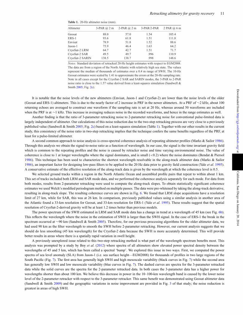
Table 1. 20-Hz altimeter noise (mm).
Altimeter 3-PAR @ 2 m 2-PAR @ 2 m 3-PAR/2-PAR 2 PAR @ 6 m
Geosat 88.0 57.0 1.54 105.4ERS-1 93.6 61.8 1.51 111.8Envisat 78.9 51.8 1.52 88.6Jason-1 75.9 46.4 1.63 64.2CryoSat-2 LRM 64.7 42.7 1.51 71.7CryoSat-2 SAR 49.5 49.7 .996 110.9CryoSat-2 SARIN 138.5 138.7 .998 148.6
Notes: Standard deviation of retracked 20-Hz height estimates with respect to EGM2008.The data are from a region of the North Atlantic with relatively high sea state. The valuesrepresent the median of thousands of estimates over a 0.4 m range of SWH. The 10-HzGeosat estimates were scaled by 1.41 to approximate the errors at the 20-Hz sampling rate.Note in all cases except for the CryoSat-2 SAR and SARIN modes, the 3-PAR to 2-PARnoise ratio is close to the 1.57 value derived from a least-squares simulation (Sandwell &Smith 2005; Fig. 2c).
It is notable that the noise levels of the new altimeters (Envisat, Jason-1 and CryoSat-2) are lower than the noise levels of the older(Geosat and ERS-1) altimeters. This is due to the nearly factor of 2 increase in PRF in the newer altimeters. At a PRF of !2 kHz, about 100returning echoes are averaged to construct one waveform if the sampling rate is set at 20 Hz, whereas around 50 waveforms are includedwhen the PRF is at !1 kHz. This increase in averaging reduces noise in the recorded waveforms, and hence in the range estimates as well.
Another finding is that the ratio of 3-parameter retracking noise to 2-parameter retracking noise for conventional pulse-limited data islargely independent of altimeter. Our calculations of this noise reduction due to the two-step retracking process are very close to a previouslypublished value (Sandwell & Smith 2005; Fig. 2c) based on a least-squares simulation (Table 1). Together with our other results in the currentstudy, this consistency of the noise ratio in two-step retracking implies that the technique confers the same benefits regardless of the PRF, atleast for a pulse-limited altimeter.
A second common approach to noise analysis is cross-spectral coherence analysis of repeating altimeter profiles (Marks & Sailor 1986).Through this analysis we obtain the signal-to-noise ratio as a function of wavelength. In our case, the signal is the time invariant gravity fieldwhich is common to the repeating profiles and the noise is caused by retracker noise and time varying environmental noise. The value ofcoherence is close to 1 at longer wavelengths where the signal dominates, and is small (<0.2) where the noise dominates (Bendat & Piersol1986). This technique has been used to characterize the shortest wavelength resolvable in the along-track altimeter data (Marks & Sailor1986), an important factor for designing low-pass filters to be applied to the 20 Hz data prior to gravity field construction (Yale et al. 1995).A conservative estimate of the effective resolution of the along-track data is given by the wavelength at which the coherence level is 0.5.
We selected ground tracks within a region in the North Atlantic Ocean and assembled profile pairs that repeat to within about 1 km.This set of tracks included both LRM and SAR mode data, and we performed the coherence analysis separately for each mode. For data fromboth modes, results from 2-parameter retracking were used to compute the along-track slopes. To obtain statistically significant coherenceestimates we used Welch’s modified periodogram method on multiple passes. The data were pre-whitened by taking the along-track derivative,resulting in along-track slope. The resulting coherence curves are shown in Fig. 6. We found that LRM slope acquisitions have a resolutionlimit of 27 km, while for SAR, this was at 26 km. In comparison, previously published values using a similar analysis in another area ofthe Atlantic found a 33-km resolution for Geosat, and 33-km resolution for ERS-1 (Yale et al. 1995). These results suggest that the spatialresolution of CryoSat-2-derived gravity will be at least 1.2 times better than previous models.
The power spectrum of the SWH estimated in LRM and SAR mode data has a change in trend at a wavelength of 45 km (see Fig. 6b).This reflects the wavelength where the noise in the estimation of SWH is larger than the SWH signal. In the case of ERS-1 the break in thespectrum occurred at !90 km (Sandwell & Smith 2005). Therefore, for our previous processing algorithms for the older altimeter data, wehad used 90 km as the filter wavelength to smooth the SWH before 2-parameter retracking. However, our current analysis suggests that weshould do less smoothing (45 km wavelength) for the CryoSat-2 data because the SWH is more accurately determined. This will providebetter results in areas where there is a spatially rapid variation in swell height.
A previously unexplored issue related to this two-step retracking method is what part of the wavelength spectrum benefits most. Thisanalysis was prompted by a study by Boy et al. (2012) where spectra of all altimeters show elevated power spectral density between thewavelengths of 45 and 5 km, which has been called a spectral ‘bump’. We explored this issue in two ways. First, we computed the powerspectra of sea level anomaly (SLA) from Jason-1 (i.e. sea surface height—EGM2008) for thousands of profiles in two large regions of theSouth Pacific (Fig. 7). The first area has generally high SWH and high mesoscale variability (black curves in Fig. 7) while the second areahas generally low SWH and low mesoscale variability (blue curves in Fig. 7). The dashed curves are spectra for the 3-parameter retrackeddata while the solid curves are the spectra for the 2-parameter retracked data. In both cases the 3-parameter data has a higher power forwavelengths shorter than about 100 km. We believe this decrease in power in the 10–100-km wavelength band is caused by the lower noiselevel of the 2-parameter retracker with respect to the 3-parameter retracker. This same benefit was demonstrated using Geosat altimeter data(Sandwell & Smith 2009) and the geographic variations in noise improvement are provided in Fig. 3 of that study; the noise reduction isgreatest in areas of high SWH.
at University of California, San D
iego on January 20, 2014http://gji.oxfordjournals.org/
Dow
nloaded from

12 E.S. Garcia, D.T. Sandwell and W.H.F. Smith
Figure 6. (a) Coherence versus spatial wavenumber (wavelength) for repeat along-track slope profiles in the North Atlantic (white box in Fig. 1). TheLRM/SAR coherence falls to a value of 0.5 at a wavelength of 27/26 km and a value of 0.2 at a wavelength of 22/20 km. (b) Power in SWH versus wavenumber(wavelength) for 3-parameter retracking of LRM (solid) and SAR (dashed).
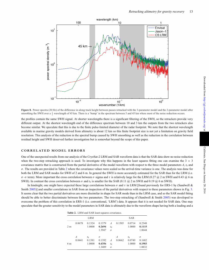
To further demonstrate the noise reduction for the 2-parameter retracker relative to the 3-parameter retracker for all the newer altimeters,we constructed power spectra of differences between the output from the two retrackers. These results are shown in Fig. 8. All the altimetersshow elevated power spectral density between the wavelengths of 45 and 5 km, which corresponds to the spectral ‘bump’ (Boy et al. 2012).The fall-off in the difference spectra for wavelengths greater than 45 km simply reflects the wavelength over which the SWH was smoothedbetween the 3-parameter and 2-parameter retracking. At longer wavelengths, both retrackers provide the same height measurement because
Figure 7. Power spectra for sea level anomaly (sea surface height minus EGM2008) as computed from Jason-1 data for two regions in the South Pacific.Dashed curves are 3-parameter retracking and solid curves are 2-parameter retracking. Black curves are from a region of generally high sea state and highmesoscale variability (longitude 190–280, latitude –55 to –35, 5500 passes of length 2048). Blue curves are from a region of generally low sea state and lowmesoscale variability (longitude 210–285, latitude –25 to –4, 4200 passes of length 2048). Inset histograms show differences in sea state characteristics. Therapid spectral roll-off at 10 km wavelength is caused by a low-pass filter applied to the 20 Hz data prior to resampling at 5 Hz. The spectral ‘bump’ is moreapparent for the 3-parameter retracked data than the 2-parameter retracked data. The spectra are smooth because they each represent about 10 million, 5 Hzobservations.
at University of California, San D
iego on January 20, 2014http://gji.oxfordjournals.org/
Dow
nloaded from
Retracking altimetry for gravity recovery 13
Figure 8. Power spectra (20 Hz) of the difference in along track height between passes retracked with the 3-parameter model and the 2-parameter model aftersmoothing the SWH over a 1
2 wavelength of 45 km. There is a ‘bump’ in the spectrum between 5 and 45 km where most of the noise reduction occurs.
the profiles contain the same SWH signal. At shorter wavelengths there is a significant filtering of the SWH, so the retrackers provide verydifferent output. At the shortest wavelength end of the difference spectrum between 10 and 3 km the outputs from the two retrackers alsobecome similar. We speculate that this is due to the finite pulse-limited diameter of the radar footprint. We note that the shortest wavelengthavailable in marine gravity models derived from altimetry is about 12 km so this finite footprint size is not yet a limitation on gravity fieldresolution. This analysis of the reduction in the spectral bump caused by SWH smoothing as well as the reduction in the correlation betweenresidual height and SWH deserved further investigation but is somewhat beyond the scope of this paper.
C O R R E L AT E D M O D E L E R RO R S
One of the unexpected results from our analysis of the CryoSat-2 LRM and SAR waveform data is that the SAR data show no noise reductionwhen the two-step retracking approach is used. To investigate why this happens in the least squares fitting one can examine the 3 * 3covariance matrix that is constructed from the partial derivative of the model waveform with respect to the three model parameters A, t0 and$ . The results are provided in Table 2 where the covariance values were scaled so the arrival-time variance is one. The analysis was done forboth the LRM and SAR modes for SWH of 2 and 6 m. In general the SWH is more accurately estimated for the SAR than for the LRM (i.e.$–$ term). More important the cross correlation between $ sigma and # is relatively large for the LRM (0.27 @ 2 m SWH and 0.43 @ 6 mSWH). In contrast the cross correlation between $ and t0 is smaller for the SAR (0.11 @ 2 m SWH and 0.19 @ 6 m SWH).
In hindsight, one might have expected these large correlations between $ and # in LRM [found previously for ERS-1 by (Sandwell &Smith 2005)] and smaller correlations in SAR from an inspection of the partial derivatives with respect to these parameters shown in Fig. 3.It seems clear that the two partial derivatives are more dissimilar in shape for SAR mode than in the LRM case, and so the SAR model fittingshould be able to better discriminate between the two parameters. The two-step retracking of (Sandwell & Smith 2005) was developed toovercome the problem of this correlation in ERS-1 (i.e. conventional, ‘LRM’) data. It appears that it is not needed for SAR data. One mayspeculate that the greater sensitivity to the model parameters in SAR data is ultimately due to the waveform shape having both a leading and a
Table 2. LRM and SAR least-squares covariance.
LRM SAR
0.0678 0.1324 0.1379 A 0.1505 0.0714 0.23482 m 1.0000 0.2694 t0 1.0000 0.1115
1.3947 $ 1.0644
A t0 $ A t0 $
0.0441 0.1381 0.1392 A 0.0662 0.0749 0.16826 m 1.0000 0.4356 t0 1.0000 0.1903
1.3489 $ 1.0832
at University of California, San D
iego on January 20, 2014http://gji.oxfordjournals.org/
Dow
nloaded from

14 E.S. Garcia, D.T. Sandwell and W.H.F. Smith
trailing edge that changes with $ , whereas in our formulation the slope of the trailing edge of the conventional LRM waveform is unaffectedby this parameter.
C O N C LU S I O N S
To measure marine gravity anomalies at an accuracy under 1 mGal, the error in the along-track slopes from the altimeter profiles must beabout 1 µrad, or there must be enough repeated tracks to achieve the 1 µrad accuracy. This study compiles several contributions towards thisgoal.
We have shown that a simple analytic function, which we derived to model CryoSat-2 SAR-mode waveforms, may be used to estimatealong-track sea surface slope. This is in spite of the fact that the model does not account for the multilook averaging applied in assemblingthe SAR waveforms. We then calculated the range precision at 20 Hz for a large set of altimeter profiles collected in SAR mode and foundthat it was almost two times better than earlier noise levels for ERS-1 and Geosat.
Two-step retracking was originally developed specifically for ERS-1 data (Sandwell & Smith 2005), but we have established that thismethod also results in a factor of 1.5 improvment in range precision for pulse-limited altimetry waveforms for other missions. Yet we foundno noise reduction from the second pass of retracking in the CryoSat-2 SAR- and SARIN-mode data. The range precision gained throughthe two-step retracking algorithm occurs over the 5–45-km wavelength band, which reduces the observed ‘bump’ in the sea level anomalypower spectrum. The 1.5 times improvement in range precision from the 2-step retracking, combined with the 1.4 times improvement in rangeprecision due to the increased PRF of the newer altimeters, results in an overall factor of 2 improvement in range precision.
Taken together, advancements from SAR altimetry, as well as the application of two-step retracking to conventional altimetry, yieldenhanced recovery of sea surface slopes from CryoSat-2, Envisat, and Jason-1 data when compared to previous measurements from thegeodetic missions of the Geosat and ERS-1 altimeters.
A C K N OW L E D G E M E N T S
We thank Salvatore Dinardo of ESA ESRIN for providing simulation results for the CryoSat-2 SAR waveforms from the SAMOSA project. Wethank the reviewers for their constructive criticism. Pierre Thibaut provided guidance in the finer points of processing Jason-1 and CryoSat-2waveforms. We thank Robert Cullen for providing early access to the oversampled SAR waveform data. We thank Jerome Benvenistefor encouraging us to use CryoSat-2 altimetry for gravity field improvement. Walter H.F. Smith contributed to the derivation provided inAppendix A and helped to refine the other sections of the paper. The retracked CryoSat-2 SAR data were kindly provided by Nicolas Picotthrough the AVISO server. The CryoSat-2 and Envisat data were provided by the European Space agency, and NASA/CNES provided datafrom the Jason-1 altimeter. This research was supported by ConocoPhillips, the National Science Foundation (OCE-1128801), and the Officeof Naval Research (N00014-12-1-0111). The manuscript contents are solely the opinions of the authors and do not constitute a statement ofpolicy, decision, or position on behalf of NOAA or the U. S. Government.
R E F E R E N C E S
Abramowitz, M & Stegun, I.A., 1964. Handbook of Mathematical Func-tions With Formulas, Graphs, and Mathematical Tables. U.S. GovernmentPrinting Office, Washington, D.C., 1045 pp.
Amarouche, L., Thibaut, P., Zanife, O.Z., Dumont, J.-P., Vincent, P. & Steu-nou, N., 2004. Improving the Jason-1 ground retracking to better accountfor attitude effects, Mar. Geod., 27(1–2), 171–197.
Andersen, O.B., Knudsen, P. & Berry, P.A.M., 2009. The DNSC08GRAglobal marine gravity field from double retracked satellite altimetry,J. Geod., 84(3), 191–199.
Bendat, J.S. & Piersol, A.G., 1986. Random Data—Analysis and Measure-ment Procedures, 2nd edn, Wiley and Sons, 566 pp.
Boy, F., Desjonqueres, J.-D., Picot, N., Moreau, T., Labroue, S., Poisson,J.-C. & Thibaut, P., 2012. CryoSat processing prototype: LRM and SARprocessing on CNES side, In Proceedings of the Ocean Surface Topogra-phy Science Team Meeting, Venice-Lido.
Brown, G., 1977. The average impulse response of a rough surfaceand its applications, IEEE Transact. Antenn. Propag., 25(1), 67–74.
Chang, S. & Jin, J.-M., 1996. Computation of Special Functions, Wiley.Chelton, D.B., Edward, J.W. & MacArthur, J.L., 1989. Pulse Compression
and Sea Level Tracking in Satellite Altimetry. J. Atmos. Oceanic Technol.,6, 407–438.
Chelton, D.B., Ries, J.C., Haines, B.J., Fu, L.-L. & Callahan, P.S., 2001.Satellite altimetry, in Satellite Altimetry and Earth Sciences, pp. 1–131,eds Fu, L.-L. & Cazenave, A., Academic Press
Cheney, R.E., Doyle, N.S., Douglas, B.C., Agreen, R.W., Miller, L., Tim-
merman, E.L. & McAdoo, D.C., 1991. The Complete Geosat AltimeterGDR Handbook, National Geodetic Survey, NOAA.
Childers, V.A., McAdoo, D.C., Brozena, J.M. & Laxon, S.W., 2001. Newgravity data in the Arctic Ocean: comparison of airborne and ERS gravity,J. geophys. Res., 106(B5), 8871–8886.
Cotton, P.D. et al., 2010. The SAMOSA Project: assessing the potential im-provements offered by SAR altimetry over the open ocean, coastal waters,rivers and lakes, in Proceedings of the ESA Living Planet Symposium.
Dibarboure, G., Renaudie, C., Pujol, M.-I., Labroue, S. & Picot, N., 2011.A demonstration of the potential of Cryosat-2 to contribute to mesoscaleobservation, Adv. Space Res., 50, 1046–1061.
European Space Agency, 2013. CryoSat Mission online resources.Available at: https://earth.esa.int/web/guest/missions/esa-operational-eo-missions/cryosat10.1093/gji/ggt469.html (last accessed 7 June 2013).
European Space Research Institute (ESRIN) – European Space Agency andMullard Space Science Laboratory – University College London, 2013.CryoSat Product Handbook. Available at: https://earth.esa.int/web/guest/missions/esa-operational-eo-missions/cryosat10.1093/gji/ggt469.html(last accessed 7 June 2013).
Ford, P.G. & Pettengill, G.H., 1992. Venus topography and kilometer-scaleslopes, J. geophys. Res., 97(E8), 13103–13114.
Galin, N., Wingham, D.J., Cullen, R., Fornari, M., Smith, W.H.F. & Abdalla,S., 2013. Calibration of the CryoSat-2 Interferometer and Measurementof Across-Track Ocean Slope, IEEE Transact. Geosci. and Remote Sens.,51(1), 57–72.
Giles, K., Wingham, D., Cullen, R., Galin, N. & Smith, W.H.F., 2012. PreciseEstimates of Ocean Surface Parameters from CryoSat-2, in Proceedingsof the Ocean Surface Topography Science Team Meeting, Venice-Lido.
at University of California, San D
iego on January 20, 2014http://gji.oxfordjournals.org/
Dow
nloaded from

Retracking altimetry for gravity recovery 15
Gommenginger, C., Martin-Puig, C., Dinardo, S., Cotton, P.D., Srokosz, M.& Benveniste, J., 2011. Improved altimetric accuracy of SAR altimetersover ocean, in Proceedings of Ocean Surface Topography Science TeamMeeting, San Diego.
Gommenginger, C., Cipollini, P., Cotton, P.D., Dinardo, S. & Benveniste, J.,2012. Finer, better, closer: advanced capabilities of SAR altimetry in theopen ocean and the coastal zone, in Proceedings the of Ocean SurfaceTopography Science Team Meeting, Venice-Lido.
Gradshteyn, I.S. & Ryzhik, I.M., 1980. Table of Integrals, Series, and Prod-ucts, Corr. & enl. ed., Academic Press.
Hayne, G., 1980. Radar altimeter mean return waveforms from near-normal-incidence ocean surface scattering, IEEE Transact. Antenn. Propag.,28(5), 687–692.
Jensen, J.R. & Raney, R.K., 1998. Delay/Doppler radar altimeter: bettermeasurement precision, in Proceedings of the Geoscience and RemoteSensing Symposium, IGARSS 1998, IEEE International, pp. 2011–2013.
Labroue, S., Boy, F., Picot, N., Urvoy, M. & Ablai, M., 2012. First qualityassessment of the Cryosat-2 altimetric system over ocean, Adv. SpaceRes., 50, 1030–1045.
Laxon, S. & McAdoo, D.C., 1994. Arctic ocean gravity field derived fromERS-1 satellite altimetry, Science, 265(5172), 621–624.
Louis, G., Lequentrec-Lalancette, M.-F., Royer, J.-Y., Rouxel, D., Geli, L.,Maia, M. & Failot, M., 2010. Ocean gravity models from future satellitemissions, EOS, Trans. Am. geophys. Un., 91(3), 21–28.
MacArthur, J.L., Marth, J., P. C. & Wall, J.G., 1987. The Geosat radaraltimeter. Johns Hopkins APL Technical Digest, 8(2), 176–181.
Marks, K.M. & Sailor, R.V., 1986. Comparison of GEOS-3 and SEASATaltimeter resolution capabilities, Geophys. Res. Lett., 13(7), 697–700.
Maus, S., Green, C.M. & Fairhead, J.D., 1998. Improved ocean-geoid res-olution from retracked ERS-1 satellite altimeter waveforms, J. geophys.Int., 134(1), 243–253.
Olgiati, A., Balmino, G., Sarrailh, M. & Green, C.M., 1995. Gravity anoma-lies from satellite altimetry: comparison between computation via geoidheights and via deflections of the vertical, Bull. Geod., 69, 252–260.
Parker, R.L., 1973. The rapid calculation of potential anomalies, Geophys.J. R. astr. Soc., 31, 445–455.
Pavlis, N.K., Holmes, S.A., Kenyon, S.C. & Factor, J.K., 2012. The develop-ment and evaluation of the Earth Gravitational Model 2008 (EGM2008),J. geophys. Res., 117, B04406, doi:10.1029/2011JB008916.
Phalippou, L. & Enjolras, V., 2007. Re-tracking of SAR altimeter oceanpower-waveforms and related accuracies of the retrieved sea surfaceheight, significant wave height and wind speed, in Proceedings of theGeoscience and Remote Sensing Symposium, IGARSS 2007, IEEE Inter-national, pp. 3533–3536.
Picot, N., Case, K., Desai, S., Vincent, P. & Bronner, E., 2012. AVISO andPODAAC User Handbook. IGDR and GDR Jason Products, SALP-MU-M5-OP-13184-CN (AVISO), JPL D-21352 (PODAAC).
Raney, R.K., 1998. The delay/Doppler radar altimeter, IEEE Transact.Geosci. Remote Sens., 36(5), 1578–1588.
Raney, R.K., 2011. CryoSat-2 SAR mode looks revisited, IEEE Geosci.Remote Sens. Lett., 9(3), 393–397.
Raney, R.K., Smith, W.H.F. & Sandwell, D.T., 2003. Abyss-Lite: improvedbathymetry from a dedicated small satellite delay-Doppler radar altimeter,in Proceedings of Geoscience and Remote Sensing Symposium Proceed-ings, IGARSS, pp. 1083–1085.
Rodrıguez, E., 1988. Altimetry for non-Gaussian oceans: height biases andestimation of parameters, J. geophys. Res., 93, 14107–14120.
Rodriguez, E. & Martin, J.M., 1994. Assessment of the TOPEX altime-ter performance using waveform retracking. J. geophys. Res., 99(C12),24957–24969.
Sandwell, D.T., 1984. A detailed view of the South Pacific from satellitealtimetry, J. geophys. Res., 89, 1089–1104.
Sandwell, D.T. & McAdoo, D.C., 1990. High-accuracy, high-resolution grav-ity profiles from 2 years of the geosat exact repeat mission, J. geophys.Res., 95(C3), 3049–3060.
Sandwell, D.T. & Smith, W.H.F., 2005. Retracking ERS-1 altimeter wave-forms for optimal gravity field recovery, J. geophys. Int., 163(1),79–89.
Sandwell, D.T. & Smith, W.H.F., 2009. Global marine gravity from retrackedGeosat and ERS-1 altimetry: ridge segmentation versus spreading rate,J. geophys. Res., 114, 1–18.
Smith, W.H.F., 1998. Seafloor tectonic fabric from satellite altimetry, Ann.Rev. Earth Planet. Sci., 26, 697–747.
Smith, W.H.F., 2004. Introduction to this special issue on bathymetry fromspace, Oceanography, 17(1), 6–7.
Smith, W.H.F. & Sandwell, D.T., 1994. Bathymetric prediction from densesatellite altimetry and sparse shipboard bathymetry, J. geophys. Res., 99,21 803–21 824.
Smith, W.H.F. & Scharroo, R., 2011. Retracking range, SWH, sigma-naught,and attitude in CryoSat-2 conventional ocean data, in Proceedings of theOcean Surface Topography Science Team Meeting, San Diego.
Smith, W.H.F., Scharroo, R., Lillibridge, J.L. & Leuliette, E.W., RetrackingCryoSat-2 waveforms for near-real-time ocean forecast products, plat-form attitude, and other applications, in American Geophysical Union,Fall Meeting 2011, San Francisco, abstract # C53F-06.
Stenseng, L. & Andersen, O.B., 2012. Preliminary gravity recovery fromCryoSat-2 data in the Baffin Bay, Adv. Space Res., 50, 1158–1163.
Stewart, R.H., 1985. Methods of Satellite Oceanography, University ofCalifornia Press.
Temme, N.M., 2012. Section 12.8. Digital Library of Mathematical Func-tions. Release date: 2012–03–23. National Institute of Standards andTechnology. Available at: http://dlmf.nist.gov/ (last accessed 7 June2013).
Thibaut, P., Poisson, J.C., Bronner, E. & Picot, N., 2010. Relative perfor-mance of the MLE3 and MLE4 retracking algorithms on Jason-2 altimeterwaveforms, Mar. Geod., 33, 317–335.
Walsh, E.J., 1974. Analysis of experimental NRL radar altimeter data, RadioScience, 9, 711–722.
Walsh, E.J., 1982. Pulse-to-pulse correlation in satellite radar altimeters,Radio Science, 17, 786–800.
Walsh, E.J., Uliana, E.A. & Yaplee, B.S., 1978. Ocean wave heights mea-sured by a high resolution pulse-limited radar altimeter, Boundary-LayerMeteorology, 13(1–4), 263–276.
Watts, A.B., 2001. Isostasy and Flexure of the Lithosphere, Cambridge Univ.Press, 460 pp.
Wessel, P. & Chandler, M.T., 2011. The spatial and temporal distribution ofmarine geophysical surveys, Acta Geophys., 59(1), 55–71.
Wingham, D. et al., 2006. CryoSat-2: a mission to determine the fluctua-tions in Earth’s land and marine ice fields, Adv. Space Res., 37(4), 841–871.
Wingham, D.J. & Wallis, D.W., 2010. The rough surface impulse response ofa pulse-limited altimeter with an elliptical antenna pattern, IEEE Antenn.Wireless Propag. Lett., 9, 232–235.
Wingham, D.J., Phalippou, L., Mavrocordatos, C. & Wallis, D., 2004. Themean echo and echo cross product from a beamforming interferometricaltimeter and their application to elevation measurement, IEEE Transact.Geosci. Remote Sens., 42(10), 2305–2323.
Yale, M.M., Sandwell, D.T. & Smith, W.H.F., 1995. Comparison of along-track resolution of stacked Geosat, ERS 1, and TOPEX satellite altimeters,J. geophys. Res., 100(B8), 15117–15127.
A P P E N D I X A : D E R I VAT I O N O F S A R WAV E F O R M M O D E L
The model return waveform is the convolution of the combined point target response and wave height distribution PG (# ) with the area versustime function that is also called the flat surface response function S (# ).
M (# ) = PG (# ) $ S (# ) . (A1)
at University of California, San D
iego on January 20, 2014http://gji.oxfordjournals.org/
Dow
nloaded from

16 E.S. Garcia, D.T. Sandwell and W.H.F. Smith
Here, we develop an approximation to the flat surface response function and recover two dominant terms—the inverse square root of timedependence, and the exponential decay factor. This approach is similar to earlier efforts in modelling the CryoSat-2 SAR waveforms (Galinet al. 2012; Wingham & Wallis 2010). The flat surface response is proportional to the integral of the product of the beam gain pattern B (r, + )and the square of the one-way antenna gain pattern G (r, + ) over an infinitesimal ring of equivalent range:
S(# ) = H (# )C$ 0% 2"
0B (,, +) G2 (,, +) d+ (A2)
Here, , is the radial coordinate, and + is the azimuthal coordinate in a standard 2-D polar coordinate system. We have incorporated variousconstant values associated with the radar instrument design in the factor C, and $ 0 is the surface backscattering coefficient. For CryoSat-2,the antenna gain pattern can be written explicitly as
G (,, +) = G0 exp
4
"5!
(, cos + " µ)2
- 21
"
+!
(, sin + " *)2
- 22
"67
, (A3)
where G0 is the boresight antenna gain. The along-track width of the antenna pattern is -1 while the across-track width is -2. The mispointingangles are denoted by µ for pitch and * for roll. We have not included the terms related to the surface gradient because they are very smallover the ocean.
We take a somewhat different approach than that taken in (Galin et al. 2012) for specifying the beam pattern. Their formulationincorporates a Hamming weighting function that is employed by the official ESA processing routine to form the synthetic Doppler beams.Meanwhile, in an earlier section of this study, we used a simplified model where the beam pattern was approximated using rectangular regionsthat decrease in area as the inverse square root of time (eq. 16). However, in forming the synthetic beam located in the nadir direction, anarrow frequency band about the zero Doppler point is selected as a result of the SAR processing. Thus, a more realistic beam pattern wouldbe one that is represented by a sinc() function. To facilitate the evaluation of the ensuing integrals in the convolution, we approximate thisusing a Gaussian function, with -b taken to be the beam width:
B (r, + ) = B0 exp
5
"(, cos + )2
- 2b
6
(A4)
and where B0 accounts for the beam gain.Upon making the assumption that the mispointing angles are small with respect to the angular extent of the antenna gain pattern, it may
be shown that (A2) can then be approximated by
S(# ) != H (# )C0
% 2"
0exp
5
"(, cos + )2
- 2b
6
exp
4
"2
5!(, cos + )2
- 21
"
+!
(, sin + )2
- 22
"67
d+ (A5)
where the factor C0 has encapsulated several constants. This can be further manipulated using trigonometric identities,
S(# ) != C0 H (# ) exp8"r 2
2
(1- 2
b
+#
1- 2
1
+ 1- 2
2
$)9 % 2"
0exp
8"r 2
2cos 2+
(1- 2
b
+ 2#
1- 2
1
" 1- 2
2
$)9d+ (A6)
and after performing a suitable change of variables, the following integral representation of the modified Bessel function of order zero can beinvoked% 2"
0exp ("x cos .) d. = 2" I0 (x) (A7)
such that (A6) can be evaluated:
S(# ) != 4" H (# )C0 exp8",2
2
(1- 2
b
+#
1- 2
1
+ 1- 2
2
$)9I0
8,2
2
(1- 2
b
+ 2#
1- 2
1
" 1- 2
2
$)9. (A8)
A further simplification may be made if we assume that the beam width -b is narrow enough that the instrument’s travel time resolutionis insensitive to the along-track position of surface area elements within the beam, allowing for the use of the asymptotic form
I0 (x) + (2"x)"1/2 exp(x). (A9)
Applying (A8) leads to
S(# ) + C1 H (# )1,
exp#
",2
- 22
$, (A10)
where again we have collapsed the preceding constants into a single factor C1. Rewriting this in terms of # by recalling (eq. 6), we get
S(# ) + C2 H (# )#"1/2 exp#
" hc
- 22
#
$. (A11)
As before, outlying constants have been gathered into C2. From this expression we see that we recover the inverse square root of timedependence, as well as get an exponential decay factor. The decay rate is dependent on the across-track width of the antenna gain pattern.
at University of California, San D
iego on January 20, 2014http://gji.oxfordjournals.org/
Dow
nloaded from
Retracking altimetry for gravity recovery 17
If we assume a Gaussian functional form for both the point target response and the surface roughness distribution, then the convolutionleading to the waveform model can be approximately written as the following integral, which is similar in form to (eq. 17):
M (# ) = PG (# ) $ S (# ) + C3
% &
"&H
&# '' # '"1/2 exp
#" hc
- 22
# '$
exp
!" (# " # ')2
2$ 2
"
d# ', (A12)
where C3 is the product of several constants. After a bit of algebra one arrives at
M (# ) = C3 exp#"# 2
2$ 2
$% &
0# '"1/2 exp
("
#1
2$ 2
$# '2 "
#hc
- 22
" #
$ 2
$# '
)d# ' (A13)
Note that this integral can be performed analytically using the following formula (Gradshteyn & Ryzhik 1980)% &
0# '"1/2 exp
&"p# '2 " q# '' d# ' = (2p)"1/4 /
#12
$exp
#q2
8p
$D"1/2
#q%2p
$, (A14)
where D"1/2 (x) is the parabolic cylinder function and / (x) is the gamma function for some argument x. Note that / (1/2) = " 1/2. We makethe substitutions p = 1/(2$ 2) and q = (hc/- 2
2 ) " (#/$ 2) so the integral becomes
% &
0# '"1/2 exp
("
#1
2$ 2
$# '2 "
#hc
- 22
" #
$ 2
$# '
)d# ' = C4$
1/2 exp
514
#hc
%- 22
$
$26
* exp#
"12
hc
%- 22
#
$exp
#" # 2
4$ 2
$D"1/2
#hc
%- 22
$ " #
$
$exp
## 2
4$ 2
$D"1/2
#hc
%- 22
$ " #
$
$(A15)
Skipping some details, the final result is
M (# ) + C4$1/2 exp
#"1
2hc
- 22
$
$exp
#"1
2hc
- 22
#
$exp
#" # 2
4$ 2
$D"1/2
#hc
- 22
$ " #
$
$. (A16)
We take the term hc$/- 22 to be small, and thus the term exp
&"hc$/2- 2
2
'can be treated as being close to a constant, and the only
remaining term for the argument of the parabolic cylinder function would then be –# / $ . Upon combining constants, we arrive at
M (# ) + A$ 1/2 exp#
" # 2
4$ 2
$D"1/2
+" #
$
,exp ("'# ) , (A17)
where ' = hc/2- 22 . This is the model provided in eq. (18) of the paper. The parameter A is related to the maximum amplitude of the recorded
waveform.As in the case of the Brown model, we would like to compute the partial derivatives of the model with respect to t0, $ and A. The
derivative of the model with respect to the amplitude parameter A is simply
( M( A
= MA
. (A18)
To compute the other derivatives we make use of the identity (Temme 2012)
(
(z
(exp
#" z2
4
$D"1/2 (z)
)= " exp
#" z2
4
$D1/2 (z) . (A19)
Now, we let z = "#/$ . Using the chain rule, the derivative with respect to t0 becomes
( M(t0
= ( M(z
(z(t0
, (A20)
where (z(t0
= 1$
upon recalling that # = t " t0.Using the expression above, the derivative of the model with respect to z is
( M(z
= "A$"1/2 exp#
" z2
4
$D1/2 (z) . (A21)
Combining terms one gets
( M(t0
= A$"3/2 exp#
" z2
4
$D1/2 (z) . (A22)
A similar approach can be used to calculate the derivative with respect to $ .
( M($
= ( M(z
(z($
. (A23)
at University of California, San D
iego on January 20, 2014http://gji.oxfordjournals.org/
Dow
nloaded from

18 E.S. Garcia, D.T. Sandwell and W.H.F. Smith
By rewriting the waveform model as M = A$"1/2 exp+" z2
4
,D"1/2 (z), we can then form the derivative from the sum of two terms. The first
term is#
( M($
$
1
= "12
A$"3/2 exp#
" z2
4
$D"1/2 (z) . (A24)
The second term is#
( M($
$
2
= "A#$"5/2 exp#
" z2
4
$D1/2 (z) . (A25)
Recalling that (z($
= #$ 2 , and then by combining terms we find that
( M($
=#
( M($
$
1
+#
( M($
$
2
= "A$"3/2 exp#
"14
z2
$ (12
D"1/2 (z) + #
$D1/2 (z)
). (A26)
The results are summarized in eqs (19)–(22) of the paper.To obtain numerical values of the parabolic cylinder functions, we use Fortran subroutines that are based on a library for the computation
of special functions (Chang & Jin 1996). The algorithms, in turn, are derived from polynomial approximations for certain ranges of theargument values as specified in (Abramowitz & Stegun 1964). The subroutines were modified slightly to evaluate the entire expressionexp("z2/4)D"1/2(z) instead of just D"1/2(z).
A P P E N D I X B : A S S E S S M E N T O F A P P ROX I M AT E S A R M O D E L
Our approximation of the SAR waveform model shape is derived under the assumptions that: (1) only the nadir-looking Doppler beamcontributes significantly to the multilooked waveform; (2) mispointing of the antenna is small compared to the antenna beamwidth; (3) thehalf-width of the nadir-looking Doppler beam is very narrow compared to the radius of the pulse-limited circle. It is clear from Fig. 4 thatour model is not correctly fitting the ‘toe’ of the waveform at the onset of the rise of the leading edge, and from Fig. 5 that our model is notestimating very low values of SWH. In this appendix we compare our model to synthetic waveforms generated from a complete simulationof all of the important complications in both single-looked (at nadir) and multilooked SAR waveforms (Cotton et al. 2010).
The SAMOSA waveform model (Gommenginger et al. 2012) was developed from physical principles, leading to a simple analyticalformulation to generate 2-D delay Doppler arrays of return power. Doppler beamforming and multilook averaging are then applied, resultingin a model that is a function of delay time and dependent on the parameters of SWH, backscatter and the roll and pitch mispointing angles.
Mispointing and multilooking can have important effects on the shape of the model waveform (Wingham et al. 2004; Cotton et al.2010). To date there is no completely analytical expression for the shape of the multilooked SAR model waveform and its partial derivativeswith respect to arrival time, SWH and off-nadir pointing angle. Computation of a fully accurate model (Phalippou & Enjolras 2007) involvesmultiple numerical integrations and thus the only practical retracking approach will involve pre-computing models and partial derivativesfor a suite of model parameters and building a retracking code that rapidly retrieves template models. This purely numerical approach willrequire extensive development and testing. Our aim is to avoid this heavy computation burden by making simplifications adequate for seasurface slope recovery. We stress that we are not trying to recover fully calibrated sea surface height, SWH or backscatter. This is in contrastto other efforts, such as the CNES Cryosat Processing Prototype (Labroue et al. 2012), that enlist numerical methods to estimate all theseparameters.
We show next that under certain conditions of moderate SWH and small off-nadir pointing angle, our analytic model (eq. 18) is adequatefor estimating along-track slope to better than 1 µrad. Moreover because the formulation has analytic derivatives with respect to the modelparameters, we can retrack 12 months of CryoSat-2 SAR waveforms in about a day on a desktop computer. This rapid analysis enables usto explore and refine least-squares approaches and waveform weighting functions as well as parameter reduction approaches (e.g. Sandwell& Smith 2005). We have found that whether for LRM or SAR-mode data, subtle factors such as the number of 20 Hz waveforms thatare assembled in a single least-squares fit or the amount of along-track smoothing of the SWH between the 3-parameter and 2-parameterretracking can have a significant effect on the along-track slope precision.
To assess the accuracy of the simple analytical model for estimating waveforms, we used our approach to retrack waveforms generatedfrom the full-multilooked theoretical model including variations in SWH (0.5–8 m), and off-nadir roll angle (0.0)–0.30); Salvatore Dinardo2012, personal communication, SAMOSA Project). The simulated waveform data was provided at a sampling of 1.5625 ns (or half theoriginal tracking gate interval) to match the new L1b SAR format being provided by ESA in ground processor version ‘B’. The first testinvolved retracking a single-looked (nadir Doppler beam only) SAMOSA waveform over the range of SWH and off-nadir roll angle shownin Fig. B1(a). When the off-nadir roll is 0), the analytic model and SAMOSA model waveforms agree in shape to better than 1 part in 1000at all gates for the full range of SWH. An exponential trailing edge decay function of the form exp ("#/') was used to improve the fit wherethe best-fit ' was 0.0149 gate"1. The arrival time estimated from the fit of the analytical model to the nadir-pointing SAMOSA data agreedto better than 1 mm in absolute range. The $ parameter from the least-squares model fit shows a good linear relationship with the SWH forthe SAMOSA data with a misfit at smaller SWH due to the detailed shape of the point target response function not being fully characterizedby our Gaussian analytic formulation. This comparison confirms that our model is a good description of the single-look, nadir-pointing case.
at University of California, San D
iego on January 20, 2014http://gji.oxfordjournals.org/
Dow
nloaded from
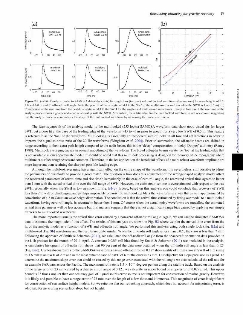
Retracking altimetry for gravity recovery 19
Figure B1. (a) Fit of analytic model to SAMOSA data (black dots) for single look (top row) and multilooked waveforms (bottom row) for wave heights of 0.5,2.0 and 6.0 m and 0) off-nadir roll angle. Note the poor fit of the analytic model to the ‘toe’ of the multilooked waveform when the SWH is low (0.5 m). (b)Comparison of the rise time from the best-fit analytic model to the SWH for the single- and multilooked waveforms. Except at low SWH, the rise time of theanalytic model shows a good one-to-one relationship with the SWH. Meanwhile, the relationship for the multilooked waveform is not one-to-one suggestingthat the analytic model accommodates the shape of the multilooked waveform by increasing the model rise time $ .
The least-squares fit of the analytic model to the multilooked (253 looks) SAMOSA waveform data show good visual fits for largerSWH but a poor fit at the base of the leading edge of the waveform (–15 to –5 ns prior to epoch) for a very low SWH of 0.5 m. This featureis referred to as the ‘toe’ of the waveform. Multilooking is essentially an incoherent sum of looks in all fore and aft directions in order toimprove the signal-to-noise ratio of the 20 Hz waveforms (Wingham et al. 2004). Prior to summation, the off-nadir beams are shifted inrange according to their extra path length compared to the nadir beam; this is the ‘delay’ compensation in ‘delay-Dopper’ altimetry (Raney1988). Multilook averaging causes an overall smoothing of the waveform. The broad off-nadir beams create the ‘toe’ at the leading edge thatis not available in our approximate model. It should be noted that this multilook processing is designed for recovery of ice topography wheremultimeter surface roughnesses are common. Therefore, in the ice application the beneficial effects of a more robust waveform amplitude aremore important than retaining the sharpest possible leading edge.
Although the multilook averaging has a significant effect on the entire shape of the waveform, it is nevertheless, still possible to adjustthe parameters of our model to provide a good match. The question is how does this adjustment of the wrong-shaped analytic model affectthe recovered parameters of arrival time and rise time? Remarkably, in the case of zero roll angle, the recovered arrival time agrees to betterthan 1 mm with the actual arrival time over the full range of SWH. However, the estimated rise time is overestimated with respect to the trueSWH, especially when the SWH is low as shown in Fig. B1(b). Indeed, based on this analysis one could conclude that recovery of SWHless than 2 m will be challenging and perhaps impossible because the multilooking blurs the waveform in a way that is well approximated byconvolution of a 2-m Gaussian wave height distribution. The conclusion is that the arrival time estimated by fitting our model to a multilookedwaveform, having zero roll angle, is accurate to better then 1 mm. Of course when the actual noisy waveforms are modelled, the estimatedarrival time parameter will be less accurate but this analysis suggests that there is not a significant range bias caused by applying our simpleretracker to multilooked waveforms.
The more important issue is the arrival time error caused by a non-zero off-nadir roll angle. Again, we can use the simulated SAMOSAdata to estimate the magnitude of this effect. The results of this analysis are shown in Fig. B2 where we plot the arrival time error from thefit of the analytic model as a function of SWH and off-nadir roll angle. We performed this analysis using both single look (Fig. B2a) andmultilooked (Fig. 9b) waveforms and the results are quite similar. When the off-nadir roll angle is less than 0.02), the error is less than 7 mm.Following the approach of Smith & Scharroo (2011), we calculated the off-nadir roll angle from the spacecraft orientation data provided inthe L1b product for the month of 2011 April. A constant 0.085) roll bias found by Smith & Scharroo (2011) was included in the analysis.A cumulative histogram of off-nadir roll shows that 90 per cent of the data were acquired when the off-nadir roll angle is less than 0.12)
(Fig. B2c). Our least-squares fits to the SAMOSA waveforms having off-nadir roll of 0.12) show misfits of 1 mm error at SWH of 1 m risingto 3.6 mm at an SWH of 2 m and in the most extreme case of SWH of 6 m, the error is 23 mm. Our objective for slope precision is 1 µrad. Todetermine the maximum slope error that could be caused by this range error associated with the roll angle we also calculated the roll rate foran example SAR pass across the Pacific. The maximum roll rate is 1.5 * 10"4 degrees per km along the satellite track. Based on the analysisof the range error of 23 mm caused by a change in roll angle of 0.12), we calculate an upper bound on slope error of 0.029 µrad. This upperbound is 35 times smaller than our accuracy goal of 1 µrad so this error source is not important for construction of marine gravity. However,it is likely and possible to have a range error of 23 mm over the length of a few thousand kilometres. This magnitude of error is significantfor construction of sea surface height models. So, we reiterate that our retracking approach, which does not account for mispointing error, isadequate for measuring sea surface slope but not height.
at University of California, San D
iego on January 20, 2014http://gji.oxfordjournals.org/
Dow
nloaded from
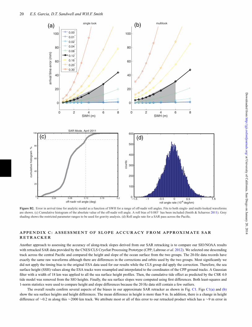
20 E.S. Garcia, D.T. Sandwell and W.H.F. Smith
Figure B2. Error in arrival time for analytic model as a function of SWH for a range of off-nadir roll angles. Fits to both single- and multi-looked waveformsare shown. (c) Cumulative histogram of the absolute value of the off-nadir roll angle. A roll bias of 0.085) has been included (Smith & Scharroo 2011). Greyshading shows the restricted parameter ranges to be used for gravity analysis. (d) Roll angle rate for a SAR pass across the Pacific.
A P P E N D I X C : A S S E S S M E N T O F S L O P E A C C U R A C Y F RO M A P P ROX I M AT E S A RR E T R A C K E R
Another approach to assessing the accuracy of along-track slopes derived from our SAR retracking is to compare our SIO/NOAA resultswith retracked SAR data provided by the CNES/CLS CryoSat Processing Prototype (CPP; Labroue et al. 2012). We selected one descendingtrack across the central Pacific and compared the height and slope of the ocean surface from the two groups. The 20-Hz data records haveexactly the same raw waveforms although there are differences in the corrections and orbits used by the two groups. Most significantly wedid not apply the timing bias to the original ESA data used for our results while the CLS group did apply the correction. Therefore, the seasurface height (SSH) values along the ESA tracks were resampled and interpolated to the coordinates of the CPP ground tracks. A Gaussianfilter with a width of 18 km was applied to all the sea surface height profiles. Then, the cumulative tide effect as predicted by the CSR 4.0tide model was removed from the SIO heights. Finally, the sea surface slopes were computed using first differences. Both least-squares and1-norm statistics were used to compare height and slope differences because the 20 Hz data still contain a few outliers.
The overall results confirm several aspects of the biases in our approximate SAR retracker as shown in Fig. C1. Figs C1(a) and (b)show the sea surface heights and height differences. The mean difference in height is more than 9 m. In addition, there is a change in heightdifference of !0.2 m along this !2000 km track. We attribute most or all of this error to our retracked product which has a !9 m error in
at University of California, San D
iego on January 20, 2014http://gji.oxfordjournals.org/
Dow
nloaded from

Retracking altimetry for gravity recovery 21
Figure C1. (a) Sea surface height in metres from the CNES/CLS (red) and SIO/NOAA (blue) retracking estimates, with the tide effect removed then filteredat 18 km. (b) Height differences have a !9 m bias and a !0.2 m height change along the 2000-km long pass. (c) Sea surface slope in microradian from theCNES/CLS (red) and SIO (blue) retracking estimates filtered at 18 km. (d) Slope differences have very small biases and trends. Histograms and statistics fordifferences between CNES and SIO (e), SIO and MSS (f) and CNES and MSS (g).
absolute height and a significant change in along-track height error, perhaps due to the differences in tide models, other corrections, or timingbias. Such errors would be unacceptable for any application using sea surface height or sea level anomaly. However note that the "0.2 merror distributed over 2000 km amounts to a slope error of only "0.1 µrad, which is well below a significant error for gravity applications.
The magnitude of the slope error due to differences in data processing are shown in Figs C1(c)–(e). The median difference in slope is"0.115 µrad (Fig. C1e) in accordance with the overall slope seen in the height difference plot (Fig. C1b). The standard deviation and medianabsolute deviation are around 2 µrad and 1.66 µrad, respectively. Figs C1(c) and (d) show that the slopes are in good agreement at lengthscales greater than about 50 km but have differences at smaller length scales due to differences in the retrackers. In addition to comparingthe along track slope from the two groups, we also compared the along-track slope from each group with the corresponding slope from theCNES/CLS 2010 mean sea surface (MSS) height model. The median absolute deviations for the CNES and SIO groups are 2.30 µrad and2.64 µrad, respectively. The main conclusion is that the differences in slope between the CNES and SIO products are smaller than theirindividual differences from the best available MSS so these independent products have excellent agreement for along-track slope.
at University of California, San D
iego on January 20, 2014http://gji.oxfordjournals.org/
Dow
nloaded from