Geophysical Investigations II - Magnetotelluric measurements

CHAPTER 6

6.1

Geophysical Investigations II - Magnetotelluric measurements for determining the subsurface

salinity and porosity structure of Amchitka Island, Alaska1

SUMMARY

The hydrogeology of small islands such as Amchitka is characterized by a layer of freshwater overlying a saltwater layer. The freshwater is derived from rainfall and discharges offshore. The salt water is typically stagnant and a dynamic balance determines the depth of the fresh to saltwater interface. Often the change from fresh to saltwater takes place over a broad transition zone, with gradually increasing salinity deeper beneath the surface.

Hydrogeological modeling of the groundwater system has provided estimates of the timing and quantities of radionuclides that could be released from the underground nuclear explosions on Amchitka Island. A key variable in this modeling is the depth of the fresh to salt water transition. However, there is very little data available to constrain hydrogeological models of Amchitka Island. Deep salinity measurements were made in a few boreholes prior to the underground explosions. Remote sensing of subsurface electrical resistivity using electromagnetic exploration methods is a complementary technique for mapping the salinity and porosity of the subsurface. The magnetotellurics (MT) method uses naturally occurring radio waves with frequencies 1000-0.001 Hz to determine the resistivity of the Earth.

During the 2004 CRESP Amchitka Island Expedition, magnetotelluric data were collected on profiles that passed across each of the three test sites. The specific questions to be addressed were:

1. What is the depth of the fresh-salt water interface at each test shot?

2. Can subsurface features associated with the underground nuclear testing

be imaged with MT?

3. Can faults be detected through their effects on groundwater flow? After processing the MT data, two-dimensional models of subsurface

electrical resistivity were derived. These showed that a pattern of increasing, decreasing and increasing resistivity was observed at each test site on Amchitka Island. The depth at which resistivity begins to decrease approximates the top of the transition zone as the salinity increases. The deeper increase in resistivity corresponds to the base of the transition zone (TZ), as salinity remains constant and the decreasing porosity causes a rise in resistivity. The following depths 1 This chapter is a condensation of Appendix 6.A authored by Martyn Unsworth, Wolfgang Soyer and Volkan Tuncer, Department of Physics and Institute for Geophysical Research, University of Alberta, Edmonton, Alberta, T6G 0B9, CANADA

Magnetotelluric Measurements For Determining The Subsurface Salinity And Porosity Structure Of Amchitka Island, Alaska

6.2

were derived from the resistivity models, and uncertainties were estimated in some parameters: Shot

depth (m)

Salinity at shot (g/liter)1

Top of TZ(m)

Top of TZ Possible range(m)

Base of TZ(m)

Base of TZ Possible range(m)

Milrow 1200 20 900 800-1100 1700 1500-2100 Long Shot 700 10 600 500-1000 1700 1500-2000 Cannikin 1700 5 900 800-1000 2500 2000-2700

1. Saliniity is measured by chloride concentration which is usually < 700 g/liter (parts per thousand) in fresh water (and 19.3 mg/liter in pure salt water or by total solute (35 g/liter or ppt) in saltwater.

The MT data processing was repeated with a range of control parameters, and several independent software packages were used. In each case, the same basic results were obtained. Subject to the limits of the data analysis, it appears that each of the underground nuclear explosions was located in the transition zone from fresh to saltwater. This implies shorter transit times to the marine environment than if the shots were located in the saltwater layer, and longer than if in the freshwater layer. Inferred effective porosities are around 30% at the surface, decreasing to 2-3% at 3000 m. This is higher than values assumed in several hydrogeological models, thus giving longer transit times for radionuclides. 1. INTRODUCTION 1.1 Objectives

As part of the CRESP Amchitka Island environmental evaluation in 2004, geophysical data were collected on the island to provide improved understanding of on subsurface structure and to provide the constraints or boundary conditions for modeling. Prior to the 2004 survey, the depth at which the transition from fresh to salt water occurred was not well known, and is a key parameter in determining transit times for contaminant migration from the test shots to the marine environment. The on-island geophysical work in 2004 focused on electromagnetic (magnetotelluric) imaging that mapped subsurface electrical resistivity. This approach gives direct constraints on the subsurface porosity and salinity of the groundwater as a function of depth and provides constraints for hydrogeological modeling. The 2004 fieldwork was designed to address the following questions:

1. What is the depth of the fresh-salt water interface at each test shot?

The hydrogeological modeling (Hassan et al, 2002) of subsurface flow on Amchitka uses assumptions of subsurface salinity and porosity as inputs. However, prior to 2004 the available hydrogeological data was quite limited, since just a few boreholes were drilled on the island. Possible transit times for

CHAPTER 6

6.3

radionuclides from the shot cavities to the marine environment are very sensitive to subsurface salinity and porosity, and geophysics can provide estimates of these parameters.

Based on hydrogeological data available from drilling conducted prior to the underground tests, and other studies of coastal hydrogeology, it was anticipated that a fresh water layer would be present at the surface, with an underlying layer of salt water. Limited data are available to determine the depth of this salt water layer and the transition zone from fresh to salt on Amchitka Island. The primary goal of the MT survey was to determine the depth of this interface at each test site and map depth variations across the island.

2. Can subsurface features associated with nuclear testing be imaged with MT?

Zones of fracturing, such as the cavity and collapse chimney, would be

expected to have a lower resistivity, owing to the enhanced porosity. It was expected that such features might be observed, especially for the Cannikin test. Also, a plume of contaminated groundwater might be discernable in the resistivity model as a region of low resistivity.

3. Can faults be detected through their effects on groundwater flow? Hydrogeological models have been used to determine the likely flow patterns and leakage times on Amchitka Island (Hassan et al, 2002). The predictions made by these models are very sensitive to the presence of faults in the near surface geological section. Faults can act as both, seals or conduits with enhanced porosity and hydraulic conductivity (Caine et al, 1997). The effect of these faults has been detected in a number of MT studies. This includes characterization at the Sellafield site in the United Kingdom (Unsworth et al, 2000) and studies of the San Andreas Fault in California (Unsworth et al., 1997. Thus it was anticipated that the Amchitka MT survey might reveal if the hydrogeology is influenced by faults that are adjacent to the underground test sites. 1.2 Electrical resistivity and coastal hydrogeology The electrical resistivity of the upper few kilometers of the Earth’s upper crust is largely controlled by the presence of interconnected aqueous fluids. The resistivity of a rock formation is a function of four parameters:

(1) The salinity of the groundwater (2) The porosity (i.e. the fraction or percent) of the rock that is occupied by a

fluid) (3) The degree of interconnection of the fluid (i.e. does the fluid form a

connected network through the medium, or is it in isolated pockets)


6.4

(4) The resistivity of the host rock This is illustrated by a set of theoretical calculations in Figure 6.1. This study represents a typical coastal location, and represents the subsurface hydrologic structure found on Amchitka Island. A freshwater layer is separated by a transition zone of increasing salinity with depth from an underlying saltwater zone. For Amchitka, a relatively high degree of interconnection is assumed, as is typical of fractured near surface rocks. Fluid resistivity (ρw) decreases through the transition zone as the salinity increases and results in a fluid resistivity profile that decreases uniformly through the transition zone and is then constant at depth in the salt water zone (Figure 6.1b). Porosity typically decreases with depth (Giles et al, 1998; Rubey and Huppert, 1959). This results in an increase in resistivity with depth that opposes the effect of increasing salinity with depth. The transition zone from fresh to salt water is expressed as a decrease in resistivity with depth (Figure 1f). The top of the salt water corresponds to the depth at which the bulk resistivity (fluid and rock) begins to increase again with depth. This is because within the transition zone, the resistivity decreases as the groundwater becomes more saline. However, within the saltwater zone, the salinity is constant at the seawater value and the decreasing porosity causes a rise in resistivity. 2. MAGNETOTELLURIC DATA COLLECTION ON AMCHITKA ISLAND IN 2004 A number of remote sensing techniques can be used to image subsurface resistivity in the upper few kilometers (McNeill, 1990). Several methods have been used in previous studies of coastal hydrogeology. For imaging at greater depths such as required for Amchitka Island, the magnetotelluric (MT) technique is the most effective. This uses naturally occurring electromagnetic signals in the frequency range (1000-0.001 Hz). MT images subsurface resistivity structure through the skin depth effect, since the depth of signal penetration is inversely related to signal frequency. Conventional broadband MT, using induction coils as magnetic field sensors and collecting data from 300 – 0.001 Hz, was used.

The magnetotelluric (MT) team consisted of the following six dedicated team members. They were assisted by the project manager for the first 5 days of data collection and as needed over the course of the operation. Personnel2 were divided into two teams for placement of MT stations. Team 1 was headed by Professor Unsworth and included Volkan Tuncer, William Shulba and Dr. Dan Volz. Team 2, headed by Dr. Soyer, included Anna Forsstrom and Chrystal Rae. Magnetotelluric (MT) data were collected on Amchitka Island in June 2004 to determine sub-surface resistivity and porosity structure. Standard techniques 2 Martyn Unsworth, Professor, University of Alberta, (U.K. / U.S.A.) Wolfgang Soyer, Post-doc, University of Alberta, (Germany) Volkan Tuncer, Doctoral student, University of Alberta, (Turkey) William Shulba ,Undergraduate, University of Alberta,(Canada) Chrystal Rae, Undergraduate, University of British Columbia, (U.K.) Anna Forsstrom, Doctoral student, University of Alaska, (Sweden)

CHAPTER 6

6.5

were used for both MT data collection and data processing. The instrumentation used was the V5-2000, a commercial system produced by Phoenix Geophysics in Toronto. MT exploration utilizes recording of both electric and magnetic fields, and thus two distinct types of MT instrumentation were used in the Amchitka Island survey. At a 3H-2E station, both magnetic and electric fields were recorded. At a 2E station, only electric fields were measured. The 3H-2E stations were moved once a day to allow for overnight recording of MT data. The 2E stations were moved several times a day to maximize productivity. The measurement of magnetic fields required digging trenches approximately 1.75 meters long by 0.3 meters wide by 0.3 meters deep for deployment of the induction coils. A post hole-digger was used to dig a vertical hole 1-1.5 meters in depth by 0.3 meters in diameter for the vertical induction coil. When the trench or hole was completed, the induction coil, weighing 20 kg, was inserted, connected and buried. The measurement of electric fields required that four lead-lead chloride electrodes be buried to a depth 0.3 meters. Electrode positions were determined by establishing the MT station center on the transect using a handheld GPS unit and then using a compass with viewfinder to lay out 50 meter lines to magnetic north, south, east and west. Electrodes positioned north to south and east to west, 100 meters apart, formed dipoles for electric field measurement. At the conclusion of field measurements at each station the electrodes and induction coils were uncovered and cleaned and each hole or trench was refilled and vegetative cover was replaced. The MT equipment was carried, as much as possible, in the flatbeds of two Polaris Rangers, on established roads. The CRESP Island Permit issued by the U.S. Fish and Wildlife Service (USFWS) did not permit off road motorized equipment, and at this time of year, early June, off road use of vehicles was impossible because of snow melt and heavy rain. Even some established roads had to be scouted thoroughly before vehicle use was permitted. The 3H-2E stations were located on MT transects less than 500 meters from roads. The 2E stations were used at locations over 500 meters from established island roads. This was to minimize the distance that heavy MT equipment for 3H-2E stations had to be carried, since these measurements required the use of heavy induction coils. All stations required carrying heavy equipment including car batteries, electrical wire, lead-lead chloride electrodes, shovels, posthole diggers and MT data recording units. The 2004 Amchitka Island survey used the two 5-channel MT systems owned by the University of Alberta, two 5-channel systems rented from Phoenix Geophysics and two 2E systems also rented from Phoenix Geophysics. Magnetic fields were recorded with MTC-30 induction coils and electric fields measured with 100 m dipoles using lead-lead chloride electrodes at each end. Prior to the survey on Amchitka Island, all six MT instruments were tested on Adak Island in a disused quarry south of the town site. This testing allowed for calibration of the MT instruments, ensured that all units were working correctly, and allowed new field crew members to be trained prior to the arrival of the expedition on Amchitka Island. It also indicated that wind noise would be an


6.6

issue in subsequent MT data collection. Broadband magnetotelluric (MT) data were collected on Amchitka Island at the 29 stations shown in Figures 6.2 and 6.3 using the Phoenix V5-2000 system. Magnetotelluric time series were generally recorded for at least 18 hours at each station, and MT data were recorded for several days at a number of locations. This field procedure allowed for multiple estimates of the magnetotelluric impedance at each frequency, and permitted the robust processing to separate signal and noise. The MT instrumentation performed well in the rugged field conditions encountered on Amchitka Island, and no units malfunctioned during the survey. Measurements of the magnetic fields were difficult owing to the strong winds that caused significant ground surface vibration. This caused the induction coils to move, and the changing component of the Earth’s static magnetic field along the axis of the coil results in magnetic noise. This type of noise can be removed through use of the remote reference technique (Gamble et al, 1979, Egbert and Booker, 1986), which requires that MT data is simultaneously recorded at two locations. On Amchitka Island the strongest noise was in the magnetic fields and due to ground motion caused by wind and ocean waves. A station separation of a few hundred meters is adequate for effective remote reference processing in this situation. On most days of the survey, all six MT units were recording simultaneously giving an array of MT data. This geometry allows for multi-station data processing, as described by Egbert (1997), and at some stations gave a modest improvement over the single remote reference results. 3. RESULTS Extensive data processing was required to resolve the subsurface salinity and porosity at each test shot based on the MT data. Several alternative mathematical models and parameter ranges were evaluated to insure that the results obtained were robust with respect to the data. Details of this methodology are provided in Appendix 6.A. 3.1 Magnetotelluric data dimensionality The geoelectric strike direction was computed using the method of Caldwell et al (2004). At frequencies below 10 Hz, a well defined strike of N55°W or N35°E was observed. Since the geometry of the low resistivity seawater dominates the resistivity structure, it is clear that an island parallel strike of N55°W is appropriate. Based on detailed analysis, the MT data from Amchitka can be considered two-dimensional (2-D), with a strike (invariant) direction approximately parallel to the axis of the island. The MT data were rotated mathematically to this co-ordinate system for all subsequent analysis.

CHAPTER 6

6.7

3.2 Magnetotelluric data modeling and inversion To interpret the MT results, the data that are a function of frequency are converted into a model of subsurface resistivity as a function of true depth. In this study, extensive 2-D inversions were used and a set of 3-D forward calculations were performed to validate this approach (Appendix 6.A). The 2-D NLCG6 inversion algorithm of Rodi and Mackie (2001) was used in this study. The NLCG6 algorithm uses non-linear conjugate gradients and is a stable algorithm that is widely used by academic and industrial geophysicists. It has been used in a number of previous studies at the University of Alberta, and the use of the algorithm is well understood. The inversion of MT data requires that additional constraints are applied to the resistivity model to give a unique solution. This process of constraining the solution is termed regularization (Tikhonov and Arsenin 1977) and generally requires that the model is spatially smooth, and/or close to a starting model. A first stage in MT data analysis was to generate a 2-D bathymetry model for each profile, provided by Mark Johnson at the University of Alaska, Fairbanks. A standard salinity was assumed for both the Bering Sea and Pacific Ocean, which yields a seawater resistivity of 0.3 mega Ohms (Ωm). A starting resistivity model was developed with a 100 Ohm-meters (Ohn-m) seafloor and the simplified bathymetry. LONG SHOT PROFILE INVERSIONS A representative inversion model for the Long Shot line is shown in the center panel of Figure 4. Figure 5 shows the measured MT data, and the apparent resistivity and phase predicted by the inversion model. Note that these two quantities are very similar, indicating that the measured MT data are well fit. The statistical fit of the data can be measured by the root-mean-square (r.m.s.) misfit. A statistically ideal fit would be unity, but a value in the range 1-1.5 is generally considered acceptable. The Long Shot model in Figure 4 has an r.m.s. misfit of 0.818 and was obtained after 195 iterations of the NLCG6 inversion algorithm. The fit of the MT data can also be displayed as residuals, which are defined as the misfit normalized by the standard error. The misfit pseudosections show that the measured MT data are generally fit to within plus or minus one standard error and that there are no systematic variations with frequency or horizontal position. This same approach was repeated for the MT data from the Milrow and Cannikin profiles. A profile of resistivity as a function of depth at the Long Shot Ground Zero is shown in Figure 6.6b (red curve). Additional curves are shown to illustrate the sensitivity of the inversion model to the most important inversion control parameters, α and τ. The following features can be identified in the resistivity model and interpreted:


6.8

Layer 1 0- 700 m Increasing resistivity Fresh water, decreasing porosity Layer 2 700-1500 m Decreasing resistivity Transition zone, Increasing salinity Layer 3 >1500 m Increasing resistivity Salt water, Constant salinity Decreasing porosity Note that the transition zone (TZ) is approximately defined as the zone where resistivity decreases with depth as salinity increases. This region is sketched on Figure 6.4 and also indicated in Figure 6.6. The top of the salt water layer is located at the depth where resistivity begins to increase again, also indicated in both Figures 6.4 and 6.6. Milrow profile inversions The inversion model for Milrow is shown in Figure 6.4 (lower panel), using the same parameters as for the Long Shot line. The inversions were repeated for a range of α and τ values (Figure 6.6a) and strike directions (Figure 6.7a). Cannikin profile inversions The inversion model for the Cannikin profile is shown in Figure 6.4 (upper panel), using the same parameters as for the Long Shot line. The inversions were repeated for a range of α and τ values (Figure 6.6c) and strike directions (Figure 6.7c). 3.3 Comparison of resistivity models with resistivity logs An important step in verifying the resistivity models derived from the MT data is to compare them with resistivity measurements made in boreholes. A number of well logs were available in the vicinity of the Milrow, Long Shot and Cannikin Ground Zeros (US Army Corp of Engineers, 1965). To make an objective comparison between the resistivity model and the well log requires that the method of measurement is understood. MT exploration images subsurface resistivity from surface measurements and detects relatively large scale features. In contrast, the well log measurement is made by an instrument within the borehole, much closer to the target. As a consequence smaller scale variations in electrical resistivity can be detected. The logs shown in Figure 6.8 have been spatially smoothed by taking a running mean of resistivity as a function of depth and three separate log measurements were made in each well.

CHAPTER 6

6.9

Figure 6.8a shows the well log comparison at the Milrow ground zero. Good agreement is observed between the normal well logs and the MT derived resistivity models, with a steady increase from 20 ohm-m to 40 ohm-m. Figure 6.8b shows well EH-3 that was located close to the Long Shot ground zero. The resistivity log shows (a) decrease in resistivity from the surface to a value of approximately 10-20 Ωm at a depth of 200-300 m and (b) a steady increase in resistivity from 200-800 m depth. This basic pattern is also observed in the resistivity-depth profile derived from the MT measurements (dashed profile). However, the agreement is not as close as observed on the other Amchitka Island profiles. This poor agreement is due in part to the spatial variability in near surface resistivity structure (determined from logs in a number of wells in this area). Figure 6.8c shows a comparison of MT derived resistivity and well log information for Cannikin. The well log profiles have been spatially smoothed to allow for a more objective comparison with the MT resistivity model. Good agreement is observed between the two independent measurements of subsurface resistivity. In the upper 400 m, the resistivity is around 20 ohm-m, and this increases to 100-200 ohm-m below 600 m. In summary, this comparison verifies that subsurface resistivity values are being correctly imaged with the MT data. No major shifts in resistivity have resulted from the proximity to the low resistivity ocean. 3.4 Porosity and salinity at Long Shot and Milrow Ground zeros The resistivity models for Long Shot and Milrow clearly show a multi-layer resistivity structure. This model can be qualitatively interpreted as follows: Layer 1 0- 700 m Increasing resistivity Fresh water, decreasing porosity Layer 2 700-1500 m Decreasing resistivity Transition zone, Increasing salinity Layer 3 >1500 m Increasing resistivity Salt water, Constant salinity Decreasing porosity These results are in agreement with the salinity data measured close to the Milrow Ground Zero in well UAE-2, which reported values of salinity close to that of seawater (35 g/ litre) at a depth of 1500m. This comparison can be made quantitative at the Long Shot Ground Zero, as summarized in Figure 6.9. Figure 6.9a shows the reported salinity in terms of total dissolved solids in grams/liter (TDS) values from UAE-2 and values in between are interpolated. These data were used because deep salinity data were not available at Long Shot, owing to the shallow (700 m) wells at this


6.10

location. Below 1500 m the TDS value for seawater is used, as there is no reason to expect hypersaline brines are present in this area. The resistivity of the groundwater (ρw) was then computed using the empirical relationship of Block (2001) and is plotted in Figure 6.9b. This assumes that the resistivity of the water (in ohm-m) is given by:

ρw = 4.5 (TDS)-0.85

Note that as the salinity rises, the resistivity decreases (Figure 6.9b). The next stage of the analysis is to determine the porosity that is required to give agreement between the resistivity imaged with the MT data, and that predicted by the salinity variation in Figure 6.9a. This requires that a relationship between bulk resistivity and the rock properties (porosity, fluid resistivity and the distribution of the pore fluid) is determined. In this study Archies Law was used, which is a standard empirical relationship used in reservoir characterization. Archie (1942) discovered that an empirical relationship for the resistivity of a completely saturated rock (ρo) is given by

m

w

o F −== φρρ

where F is termed the formation factor, Φ is the porosity and ρw is the resistivity of the pore fluid. A key control parameter in Archie’s Law is the cementation factor m. Empirical studies show that this lies between 1 and 2. Typical values reported include m = 1.8-2.0 for consolidated sandstones and m=1.3 for unconsolidated sands. It can be shown that the case with m=1 corresponds to fluid distributed in cracks, while m=2 corresponds to fluid distributed in spherical, poorly connected, pores. A value of m=1.5 represents an intermediate case and is used in this study as the preferred value. Figure 9c shows the porosity variation required for agreement between the predicted and observed electrical resistivity for m=1, m =1.5 and m=2. The porosity inferred with a cementation factor of m = 1.5 is around 30% at the surface and decreasing to 2% at a depth of 3000 m. These porosity values can be evaluated by comparison with compilations of porosity-depth variations derived from well log data. Giles et al (1998) list upper and lower bounds of porosity for a range of lithologies and these are shown in Figure 10b. While the porosity values obtained for Long Shot are lower than many studies, they are certainly within the expected range of values. Most of these studies report an exponential decrease in porosity with depth, as suggested by Rubey and Hubbert (1959). It should also be noted that these porosities are in agreement with the study of core recovered from pre-test drilling on Amchitka Island (see Figure 2.3 in Hassan et al, 2002). The above calculations were repeated with other equations relating salinity to groundwater resistivity. For example, Meju, (2000) studied a location where the water resistivity (ρw) in ohm-m and TDS can be related by:

ρw = 6.12 (TDS)-1.015

CHAPTER 6

6.11

This equation was applied to the Long Shot resistivity model and the final porosities were very similar to those in Figure 6.9. The porosity was also computed using the modified brick layer model of Schilling et al (1997). This gave porosity values close to that determined for Archie’s Law with m = 1. Note that these calculations will give the lowest porosities, since they assume the highest degree of interconnection (i.e. the smallest possible amount of fluid is needed to lower the resistivity). The top of the transition zone is approximated by the depth at which resistivity begins to decrease due to increasing salinity. For Long Shot this occurs at 600 m. The base of the transition zone occurs at the depth at which the resistivity increases at depth. This occurs because the salinity has reached the seawater value and cannot increase any more. Decreasing porosity below this depth causes a rise in resistivity. Thus the MT data show that the top of the saltwater layer (the bottom of the transition zone) occurs at a depth of 1700 m below the Long Shot Ground Zero surface (Figure 6.9). Figures 6.6 and 6.7 shows the results of different inversions using varying control parameters, and indicates that this depth could be in the depth range 1500-2000 m. A similar analysis was undertaken for the Milrow ground zero, as shown in Figure 6.11. A similar porosity-depth variation was inferred. The top of the transition zone is located at 900 m. The increase in resistivity, and by inference the bottom of the transition zone (or top of the salt water layer), occurs at 1700 m at Milrow (Figure 6.11). Figure 6.6 and 6.7 suggest that this depth is in the range 1500-2100 m. In summary, the salinity data from boreholes close to the Milrow and Long Shot Ground Zero locations are consistent with the MT data. Realistic porosity values are required to give agreement with the predicted and observed subsurface resistivities. Thus the MT study confirms the hydrogeological evidence that both Long Shot and Milrow were detonated in the upper part of the transition from fresh to saltwater. One potential limitation of these calculations is that borehole salinity measurements were made prior to the underground explosions, and the geophysical measurements were made afterwards. If the explosions caused significant changes in subsurface porosity and salinity, then this may influence the calculations. 3.5 Porosity and salinity at Cannikin Ground Zero The resistivity models for Cannikin show a layered structure in the upper 4000 m of the subsurface. While the relative depth variations are similar to those observed in the Long Shot and Milrow area, the absolute resistivity values are higher, especially in the low resistivity layer between 1500 and 3000 m (Figure 6.4). This change in absolute resistivity values is real, since it is observed in both the MT models and resistivity logs (Figure 6.8). It should also be noted that salinities are significantly lower than in the Long Shot and Milrow area. At a depth


6.12

of 1500 m in the Milrow shaft a salinity of 30 g/l was observed (UAE-2). In contrast, at the base of the Cannikin shaft (about 1700 m below surface), the reported salinity is 5 g/l (UAE-1). Given the higher elevation above sea level of Amchitka Island on the Cannikin profile, it would be expected that the fresh-salt water interface would be at a greater depth than in the Long Shot and Milrow area. The analytic formula of Ghyben-Herzberg (Todd and Mays, 2005) assumes a static groundwater regime and buoyancy calculations predict the interface depth to be 40 times the surface elevation above sea level. This predicts depths of 1800-2200 m and 2800-3200 m in the Long Shot and Milrow and Cannikin areas respectively. These values are consistent with the depths previously determined from the MT data. As with the Long Shot and Milrow profiles, it is important to understand what combinations of salinity and porosity are consistent with the measured MT data. At Cannikin, the porosity can be computed in the same way as for the other profiles. However, there are uncertainties about the salinity data measured at Cannikin and an assumed porosity was used to determine the possible range of salinity values. COMPUTE POROSITY ASSUMING THE SALINITY (TDS) DATA IS KNOWN The first stage of analysis for Cannikin was to assume that the salinity (TDS) values measured in well UAE-1 for Cannikin are reliable. These TDS values are low, and it has been speculated that they reflect mixing of drilling fluids with the groundwater (Fenske, 1972). The MT data collected in this project provide a way of evaluating these TDS data. A porosity calculation was undertaken, and the results are shown in Figure 6.12. The surface value of resistivity was taken from near surface salinity measurements and below the bottom of the shaft, a linear increase to seawater values was assumed. The computed porosity is quite similar to that at Long Shot and Milrow and decreases with depth from surface values of 30% to around 3% at 3000 m depth. The porosity depth variations for the three ground zeros are shown together in Figure 6.10a. Note that the values at Cannikin are slightly higher than at Milrow and Long Shot but show a similar trend. Note the zone of essentially constant porosity between 1000 and 2000 m. Given the fact that the TDS values for Cannikin and Milrow-Long Shot were quite different, this result suggests that the computational approach is valid, as similar geological structures are expected in these two parts of the island (and hence similar porosities). It should also be noted that the porosities computed in this analysis are effective porosities. Subsurface structures often contain dual porosity systems with fluids in both networks of cracks and isolated pores. The MT exploration method uses natural electric currents to image subsurface resistivity, which is dominated by the porosity and interconnection of fluids. This effectively measures the amount of interconnected pore space. An additional perspective on the porosity values can be obtained by comparison with other studies of porosity depth variations. Giles et al (1998)

CHAPTER 6

6.13

compiled a number of datasets for varying lithologies and some of these are shown in Figure 6.10b. Maximum and minimum porosities are shown for carbonate, shale and sandstone lithologies. No adequate datasets were found for the breccia and volcanic rocks encountered on Amchitka Island, but porosities are likely to be similar, perhaps lower. Note that the porosities inferred for Amchitka Island (with a cementation factor, m = 1.5 in Archie’s Law) are low compared to the data of Giles et al (1998), but within the range of observed values. The porosity data in Figure 10b show an exponential decrease with depth, as do the other Amchitka Island models. On the basis of this analysis, the top of the transition zone at Cannikin is at a depth of approximately 900 m. The increase in resistivity that is associated with the base of the transition zone (top of salt water layer) occurs at a depth of 2500 m below the Cannikin Ground Zero. The uncertainty analysis in Figures 6 .6 and 6.7 shows that this depth could be between depths of 2000 and 2700 m. COMPUTE THE SALINITY (TDS) ASSUMING THE POROSITY DATA IS KNOWN As mentioned in the previous section, it is possible that the Cannikin salinity data are unreliable. The values at the base of the shaft are significantly below those expected for seawater and there is no evidence of the distributed rise that characterized the Milrow salinity data. To test this hypothesis, a second calculation using an alternative approach was performed. This assumed that the porosity-depth profile for Milrow was also valid for Cannikin (Figure 6.13). The computations used a cementation factor of m=1.5 in Archie’s Law and the results showed that a significant increase in salinity below 2000 m is required, likely indicating the presence of the saltwater layer. Another calculation used a simple exponential decay of porosity with depth (Rubey and Hubbert, 1959) and gave a similar result (Figure 6.14). This shows that the increase in salinity at Cannikin is not the result of the non-uniform decrease in porosity used in Figure 6.13. Thus the analysis presented above strongly suggest that at the Cannikin Ground Zero the reported salinity data in well UAe-1 are consistent with the MT for a similar porosity depth variation to that inferred in the Milrow-Long Shot area. This indicates that the Cannikin test took place in the transition zone, perhaps implying a shorter transit time to the marine environment ocean than a location in the saltwater layer, but longer than if it were completely in the fresh-water zone. It should also be noted that the transition from fresh to salt water layer is indicated by the decrease in resistivity at depth in each model in Figure 6.4. In the Cannikin model, this occurs at greater depth than for Milrow and Long Shot. At the greater depth of the Cannikin explosion, the porosity is lower and thus the relative decrease in resistivity is smaller.


6.14

3.6 Evidence for faults influencing the hydrogeology? In the study at the Sellafield site described by Unsworth et al (2000), shallow faults exhibited a strong influence on the near surface resistivity, since they acted as barriers to shallow groundwater flow. This effect is not observed on any of the resistivity models presented for Amchitka Island, which are generally spatially smooth. Rougher models can be generated from the MT data, but are not required by the MT data. Another reason for the apparent absence of fault induced resistivity variations in the resistivity models shown in Figure 6.4 is that most of the faults mapped on Amchitka Island are essentially parallel to the MT profiles. The original plan for the 2004 MT survey included profiles that were located away from the underground test sites. This would have given constraints on hydrogeology that was not influenced by the explosions, and would have also determined if cross island faults were influencing the hydrogeology. However, the short survey time on Amchitka Island did not permit these MT data to be collected.

3.7 Evidence for structures associated with the underground explosions Therefore questions regarding features produced by the underground nuclear explosions are not addressed here, and indicate the need for additional study. A fundamental limitation in answering these questions is that MT profiles were not collected in regions unaffected by the underground nuclear tests. While each MT profile shows a predominantly layered structure, there are lateral variations. These are likely due to heterogeneity with the layer, but the non-uniform station spacing can also reduce resolution. However, several features can be seen that may be related to the alteration of the subsurface, especially for the Cannikin test. These include low resistivity values in the upper 500 m of the eastern part of the Cannikin transect. In this area the profile crosses the collapse area and the surface is highly fractured, a situation that would lower the electrical resistivity. There is also a hint in Figure 6.4 that in the high resistivity layer at 1000-2000 m depth at Cannikin, there is a reduced resistivity that is spatially coincident with the chimney location. However, the station spacing does not allow this feature to be resolved with confidence. 4. Conclusions On the basis of the MT data collection, analysis and interpretation listed above, the following conclusions can be derived. It should be noted that there is inherent non-uniqueness associated with the analysis of geophysical data. Notwithstanding, the following conclusions appear to be robust in this respect:

1. At the Long Shot Ground Zero, the transition from fresh to salt water occurs in the depth range 600 to 1700 m. This implies that the Long Shot

CHAPTER 6

6.15

explosion (700m) was detonated at the top of the transition zone. 2. At the Milrow Ground Zero, the transition from fresh to salt water occurs in

the depth range 900 to 1700 m. Thus it appears that the Milrow explosion (1200m) was detonated in the middle of the transition zone.

3. At Cannikin the transition from fresh to saltwater occurs in the depth

range 900 to 2500 m. The greater depth of the saltwater layer at this location is consistent with the higher topography in this part of the island. On the basis of these values, the Cannikin shot cavity (1700m) was located in the transition zone.

4. The relatively low salinity data measured in UAe-1 prior to the Cannikin

test are consistent with the MT data. However, it should be remembered that salinity measurements in UAE-1 were made prior to the detonation and geophysical measurements were made 33 years afterwards.

5. Inferred effective porosities are around 30-40% at the surface, decreasing

to 2-3% at 3000 m. This is higher than values assumed in several hydrogeological models, thus giving longer transit times for radionuclides.

6. There is some evidence in the resistivity model for enhanced porosity that

could have been caused by enhanced fracturing in the Cannikin chimney.

7. No evidence was found for shallow faults influencing the groundwater flow. Additional MT data are needed to reliably address this question, since most faults are oriented parallel to the MT profiles. Coverage was limited owing to the short time available for MT data collection in June 2004.

Additional questions involve comparable study of reference sites unimpacted by the blasts, and closer estimation of the cementation factor M which influences porosity estimate in Archies equation. Appendix for Chapter 6 (See attached CD-ROM) 6.A. Magnetotelluric measurements for determining the subsurface salinity and porosity structure of Amchitka Island, Alaska


6.16

Figure 6.1: Theoretical study of the effect of subsurface porosity and salinity on the overall resistivity of a rock (a) Variation of salinity as a function of depth (TDS = total dissolved solids, [Seawater = 35 g/l ppt]) (b) resistivity of the ground water assuming the empirical relationship of Block (2001). (c)+(d) The porosity is constant with depth, resulting in a uniformly decreasing bulk resistivity with increasing depth. (e)+(f) Porosity decreases with depth, resulting in a more complex variation of bulk resistivity with depth. TZ = transition zone from fresh to salt water. Note that in (f) the resistivity decreases through the transition zone, and increases in the saltwater layer.

CHAPTER 6

6.17

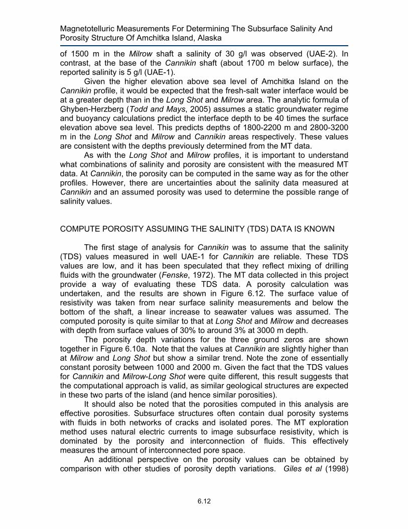
Figure 6.2: Map of Amchitka Island showing the magnetotelluric (MT) transects and bathymetry. The red triangles denote the locations of the three underground nuclear explosions.

Figure 6.3: Details of the MT survey area on Amchitka Island showing the three profiles. Ground zeros are represented by yellow triangles, 2E stations by red dots and 5-channel sites represented by blue dots. Color shading denotes elevation.


6.18

Figure 6.4: Inversion models for Long Shot, Milrow and Cannikin profiles. Long Shot model is amc_lgs_tetm_1_6_mju_a1_t3_stat_TETM; the Milrow profile model is amc_mil_tetm_1_3_mju_a1_t3_stat_TETM and the Cannikin profile model is amc_can_tetm_1_6_mju_a1_t9_stat_TETM. Asterisks show the locations of explosion cavities. The dashed lines denote the inferred location of the transition zone (TZ), defined by the downward decrease in resistivity.

CHAPTER 6

6.19

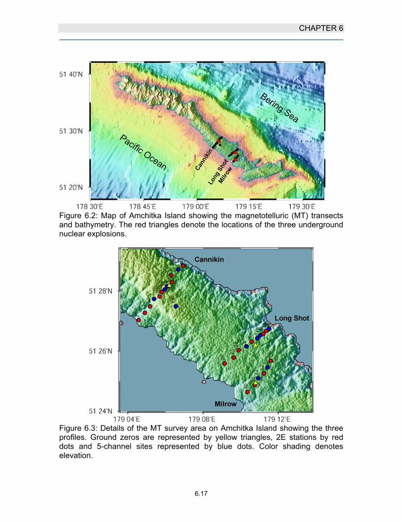
Figure 6.5: Data fit for the Long Shot profile. Data were fit with a root-mean-square (r.m.s.) misfit of 0.818 after 195 iterations.


6.20

Figure 6.6: Variation of resistivity with depth for a set of nine inversion models with different combinations of inversion control parameters. The models are shown at the ground zero for each profile and use α = [0.3, 1, 3] and τ = [1, 3, 10]. The red profile denotes the reference inversion model for α = 1 and τ = 3. Asterisks denote the depths of the explosions. TZ = transition zone.

Figure 6.7: Variation of resistivity with depth as the strike angle is varied. All inversion used α = 1 and τ = 3. The red curve is for the preferred value of N55°W. Other rotation angles are N50°W, N40°W N60°W. Note that the choice of rotation angle has little effect on the variation of resistivity with depth. Asterisks denote the depths of the explosions. TZ = transition zone.

CHAPTER 6

6.21

Figure 6.8: Comparison of resistivity model (dashed line) with well log data. The well log data has been spatially smoothed and the three curves in each well were obtained with different logging tools. Black = short normal log, blue = long normal log; red = lateral log. (a) Milrow MT profile and well UAE-2, (b) Long Shot MT profile and well EH-3, (c) Cannikin MT profile and well UAE-1. Note the good agreement between the MT model and well-log data at Cannikin and Milrow. Poorer agreement is observed at Long Shot, likely due to the variable near surface structure that is discussed in Appendix 6A.


6.22

Figure 6.9: Hydrogeology for Long Shot Ground Zero. (a) Shows the salinity (TDS) at the nearby UAe-2 well (red circles) and the blue line denotes a simplified form. The maximum value permitted is 35 g/l equivalent to seawater. (b) resistivity of the pore fluid derived from (a) using the equation of Block (2001). (c) Effective porosity required to give agreement between bulk resistivity and that determined by the MT data. Computation uses Archies’ Law with exponents m=1, 1.5 and 2 (d) Resistivity from MT data (red circles) compared to that predicted by data (blue line) in panels (a)-(c). The asterisk (*) denotes the depth of the shot cavity.

CHAPTER 6

6.23

Figure 6.10: (a) Comparison of effective porosity at the three ground zeros. Note that despite differing values of TDS, the porosities for m = 1.5 are quite similar. (b) Comparison of the m = 1.5 porosities with database values from Giles et al (1998) for carbonates, sandstone and shale. Dashed green line (carbonates), dashed blue line (sandstone) and dashed black line (shale). The porosities determined with m = 1.5 in Archie’s Law are at the lower end of the spectrum observed in other locations.


6.24

Figure 6.11: As figure 6.9, but using the MT derived resistivity for the Milrow Ground Zero. Note the similar porosities at Milrow and Long Shot. The asterisk (*) denotes the depth of the shot cavity.

CHAPTER 6

6.25

Figure 6.12: Hydrogeology for Cannikin, showing the same quantities as previous figure. Note that salinities in well UAE-1 (a) are significantly lower than observed at a similar depth for Milrow. Below the base of the emplacement shaft the salinity is assumed to rise rapidly to the seawater value of 35 g/l. The asterisk (*) denotes the depth of the shot cavity.


6.26

Figure 6.13: Hydrogeology at the Cannikin Ground Zero. The porosity depth variation from Milrow with m=1.5 was assumed and the salinity required to reproduce the variation of resistivity with depth was computed. Note that a significant increase in salinity is predicted just below the depth of the base of the Cannikin shaft. The asterisk (*) denotes the depth of the shot cavity.

CHAPTER 6

6.27

Figure 14: Hydrogeology at the Cannikin Ground Zero. An exponential porosity depth variation was assumed and the salinity required to reproduce the variation of resistivity with depth was computed. Note again that a significant increase in salinity is predicted below the depth of the shot cavity. The asterisk (*) denotes the depth of the shot cavity.


6.28

This page is intentionally left blank.

Geophysical Investigations II - Magnetotelluric measurements

Documents

Transcript of Geophysical Investigations II - Magnetotelluric measurements