Western Michigan University Western Michigan University

ScholarWorks at WMU ScholarWorks at WMU

Master's Theses Graduate College

6-1997

Geophysical Investigation of Anomalous Conductivity Associated Geophysical Investigation of Anomalous Conductivity Associated

with a Hydrocarbon Contamination Site with a Hydrocarbon Contamination Site

Mike S. Nash

Follow this and additional works at: https://scholarworks.wmich.edu/masters_theses

Part of the Geology Commons

Recommended Citation Recommended Citation Nash, Mike S., "Geophysical Investigation of Anomalous Conductivity Associated with a Hydrocarbon Contamination Site" (1997). Master's Theses. 4352. https://scholarworks.wmich.edu/masters_theses/4352

This Masters Thesis-Open Access is brought to you for free and open access by the Graduate College at ScholarWorks at WMU. It has been accepted for inclusion in Master's Theses by an authorized administrator of ScholarWorks at WMU. For more information, please contact wmu-scholarworks@wmich.edu.

I

GEOPHYSICAL INVESTIGATION OF ANOMALOUS CONDUCTIVITY

ASSOCIATED WITH A HYDROCARBON CONTAMINATION SITE

by

Mike S. Nash

A Thesis

Submitted to the

Faculty of The Graduate College in partial fulfillment of the

requirements for the

Degree of Master of Science Department of Geology

Western Michigan University

Kalamazoo, Michigan

June 1997

Copyright by

Mike S. Nash

1997

ACKNOWLEDGMENTS

It is difficult to list all of the people and institutions that have assisted me in

this research project. First off, thanks to my committee, Dr. William Sauck, Dr.

Estella Atekwana, and Dr. Alan Kehew, who provided their total support to my work.

I am also indebted to the Society of Exploration Geophysicists ,Western Michigan

University, the Graduate College, and the Department of Geology, all of which

provided funds or equipment to assist me with the research.

Secondly, I thank my able and willing assistants Mr. Darin Meyer and Ms.

Beth Pelland, who helped with much of the field work. Also, a special thanks to Mr.

D. Dale Werkema, who assisted with the field studies and critiqued much of the

analysis. Additional thanks are due to Dr. Anthony Endres and Dr. John Greenhouse,

both formerly of the University of Waterloo who provided a needed critique of the

work in progress. Special thanks are due to SERDP and NCIBRD, especially Mark

Henry and Dr. Michael Barcelona for all of the generously provided information.

Finally, I thank my brother Matty, for demonstrating to me the value of

questioning everything and for telling me to do it: "my way".

Mike S. Nash

11

..

GEOPHYSICAL INVESTIGATION OF ANOMALOUS CONDUCTIVITY

ASSOCIATED WITH A HYDROCARBON CONTAMINATION SITE

Mike S. Nash, M.S.

Western Michigan University, 1997

The high electrical conductivity measured from chemical analyses from

ground water below a hydrocarbon contaminated site was the focus of this study.

Most theoretical studies have indicated that the electrical conductivity of hydrocarbon

contamination is lower than that of the surrounding medium. Geochemical studies at

other sites have shown that areas of dissolved fuel oil plume have a higher electrical

conductivity. Six methods: Self Potential, Mise-a-la-Masse, Vertical Electrical

Sounding, Dipole-Dipole Resistivity Profiling, Electromagnetic Induction, and

Ground Penetrating Radar were all used in an attempt to see which method( s) could

identify regions of high conductivity.

The findings of this study show that the Ground Penetrating Radar, Dipole­

Dipole Resistivity Profiling and Self Potential identified conductive zones coincident

with the location of the dissolved plume. Vertical Electrical Soundings showed some

broad changes in anomalous areas, but not to high degree of resolution. The Mise-a­

la-Masse and Electromagnetic Induction techniques, as applied to this site, did not

show a conductive anomaly in areas identified by geochemical studies.

TABLE OF CONTENTS

ACKNOWLEDGEMENTS.................................................................................... 11

LIST OF TABLES ........................................................ :......................................... Vl

LIST OF FIGURES ................................................................................................ vu

CHAPTER

I. INTRODUCTION ... .......................................................................... ....... .. 1

Statement of Problem......................................................................... 1

Purpose of Study................................................................................ 2

Site History . . . .. . . . . . . . .. . . . .. . . . . . . . . . . .. . . . .. . . . .. . . . .. .. . .. .. . . . .. . . . .. . . . . . . . .. . . . . . . . . . . .. . . . . 2

Site Geology . . . .. . . . . . .. . . . .. .. . . . .. . . . .. . . . . . . . . . . .. . . . .. . . . . . . . . .. .. . . . .. . . . . . .. . . . . . .. . . . . . .. . . 3

Site Geochemistry.............................................................................. 5

II. REVIEW OF RELEVANT LITERATURE ............................................... 11

Theoretical Models . . .. .. . .. .. . . . . . .. . .. .. . .. .. . . . .. . . . . . . . . . . .. . . . .. .. . . . .. .. . . . .. . . . . . .. . . . . . 11

Controlled Spill Studies..................................................................... 13

Field Studies ...................................................................................... 15

Geochemical Studies.......................................................................... 17

III. METHODOLOGY ..................................................................................... 20

Self Potential...................................................................................... 20

Mise-a-la-masse ................................................................................. 21

Electrical Resistivity.......................................................................... 24

lll

CHAPTER

Table of Contents -- Continued

Vertical Electrical Soundings . . . . . . . . . . . . . . . . . . . . . . . . . . . . . . . . . . . . . . . . . . . . . . . .. . . 24

Dipole-Dipole Resistivity Profiling.......................................... 26

Electromagnetic Induction................................................................. 28

Ground Penetrating Radar . . .. . .. . . . .. . . . .. . . . .. . .. .. . .. .. . .. .. . .. .. . .. .. . . . .. .. . . . .. . . . .. . 30

IV. RESULTS................................................................................................... 32

Self Potential...................................................................................... 32

Mise-a-la-masse ................................................................................. 32

Electrical Resistivity.......................................................................... 35

Vertical Electrical Soundings . . . . . . . . . . . . . . . . . . . . . . . . . . . . . . . . . . . . . . . . . . . . . . . . . . . 3 5

Dipole-Dipole Resistivity Profiling.......................................... 39

Electromagnetic Induction................................................................. 45

Ground Penetrating Radar . . .. . . . .. . .. .. . .. .. . .. . . . .. . . . . . . .. . . . .. . . . . . . . . . . .. . . . .. . . . . ... . 45

V. INTERPRETATIONS ................................................................................ 50

Geophysical Results........................................................................... 50

Self Potential............................................................................. 50

Mise-a-la-masse ........................................................................ 51

Vertical Electrical Soundings .. .. ... . . ... .. ... . . .... .. .. .. ... .. ... . . .. .. . . . ... . . 52

Dipole-Dipole Resistivity Profiling.......................................... 55

Electromagnetic Induction........................................................ 59

IV

CHAPTER

Table of Contents -- Continued

Ground Penetrating Radar . . . . . . . . . . . . . . . . . . . . . . . . . . . . . . . . . . . . . . . . . . . . . . . . . . . . . . . . 62

Performance of the Methods.............................................................. 62

Conclusions and Recommendations ...... .. ...... .. .. .. .... .. .. .. .... .. .. .. .. .. .... .. 65

APPENDICES

A. Organic Chemicals Detected in July 1996.... .... .. .. .. .... .. .. .. .... .. .. .. .. .... .. .. .. .. .. 67

B. Coincident EM-31 and EM-34 Profiles...................................................... 69

C. Permission to Use NCIBRD Files .............................................................. 73

BIBLIOGRAPHY................................................................................................... 75

V

LIST OF TABLES

1. Results ofNCIBRD Chemical Analyses of FT-02 Site From April 1996.. 8

2. Inverse Models for VES # 1 ............................ :........................................... 35

3. Inverse Models for VES # 2........................................................................ 37

4. Inverse and Forward Models for VES # 3 .................................................. 39

5. Inverse Models for Each VES..................................................................... 52

6. Forward Models for Electromagnetic Induction......................................... 60

7. Results ofElectomagnetic Induction Forward Models............................... 61

Vl

LIST OF FIGURES

1. FT-02 Site Map.............................................................................................. 4

2. Topographic Map ofFT-02 Site ........................ ."........................................... 6

3. FT-02 Site Plume With Well Locations......................................................... 7

4. Electrode Configurations for Mise-a-la-masse, Vertical ElectricalSoundings, and Dipole-Dipole Profiling........................................................ 22

5. Self Potential Contour Plot............................................................................ 3 3

6. Mise-a-la-masse Contour Plots...................................................................... 34

7. Field and Inverse Model Plot for VES # 1..................................................... 36

8. Field and Inverse Model Plot for VES # 2..................................................... 38

9. Field and Inverse Model Plot for VES # 3..... .. . . . .. . . . . . .. . . . . . .. . . . . . . . .. . . . . . . . . . . . . . . . . . . 40

10. Dipole-Dipole Resistivity Profile Along Line 305 m North,10 m Dipoles... 41

11. Dipole-Dipole Resistivity Profile Along Line 305 m North, 20 m Dipoles.. 4 3

12. Dipole-Dipole Resistivity Profile Along Line 275 m North, 15 m Dipoles.. 44

1 3. EM-31 and EM-34 Profiles Along Line 305 m North................................... 46

14. GPR Profile Along Line 305 m North........................................................... 47

15. GPR Spectral Analysis for 4 Traces Along Line 305 m North...................... 49

16. Dipole-Dipole Resistivity Forward Model Without Plume........................... 57

17. Dipole-Dipole Resistivity Forward Model With Plume................................ 58

vu ..

CHAPTER I

INTRODUCTION

Statement of Problem

Contamination of shallow aquifers by fuel oils is an increasing problem in the

United States. This contamination is commonly associated with leaks from petroleum

product storage tanks or spills that occur during the handling of the petroleum. This

contamination of the shallow aquifer can ruin a water supply and, in extreme cases,

endanger regions down gradient from the contamination site. It is in the best interest

of the public to develop techniques for determining the location of contamination and,

in some cases, the specific nature of the contamination.

The intuitive electrical model for fuel oil contamination treats the fuel oil as a

electrically resistive body in a more conductive host of groundwater (Monier­

Williams, 1995). Laboratory experiments by Mazac and others (1990), DeRyck and

others (1993) and Gajdos and Kral (1995) have attempted to analyze the effect of fuel

oil contamination in the subsurface by measuring the physical properties of electrical

conductivity, electrical permittivity, and magnetic permeability. The conclusions of

most of the laboratory studies have corroborated the theoretical model. However,

field studies conducted by Western Michigan University have found instances where

1

the fuel oil contamination has appeared as an electrically conductive body (McNeil,

1994). Therefore, an analysis of the field results in comparison with the laboratory

studies must be conducted to determine the reasons for this serious discrepancy.

Gajdos and Kral, (1995) and others have also noticed conductive behavior.

Purpose of Study

Geophysical field surveys were deployed over an area of known fuel oil

contamination. Geochemical and geological background information exists for this

site, and the geophysical results can be compared to models based on the subsurface

conditions. The first objective was to determine if the dissolved fuel oil plume

contamination was electrically conductive or resistive. The second objective was to

evaluate the specific methods used in the surveys to see which are best suited for

determining contamination. This study is intended to provide a framework for

subsequent surveys to improve and supplement the various methods to a higher

degree of accuracy and precision with respect to the measurement of the physical

properties.

Site History

The site is located on the decommissioned Wurtsmith Air Force Base

(WAFB), in Oscoda, Michigan. The site itself was a former fire training facility, Fire

Training Area 02 (FT-02), used for weekly training exercises for a duration of almost

2

40 years (Barcelona, oral commun., 1996). The training exercises typically consisted

of the ignition of approximately 2000 gallons of JP-4 aviation fuel. Some but not all

of the JP-4 was consumed during the exercise, leaving the rest to either evaporate into

the air or seep into the ground below. Until the early 1980's the ground cover in the

site consisted only of grass. At that point a concrete fire pad was installed with a

drain. This drain was connected to a oil-water separator in an attempt to capture the

fuel before it seeped into the ground. Personal communications with engineers

working on the site have revealed that the drain often overflowed, leaving the JP-4

and fire fighting chemicals to seep into the ground (Barcelona, oral commun, 1996).

The FT-02 site is currently being studied under the auspices of the National Center for

Bioremediation Research and Development (NCIBRD), which is a partnership of the

Department of Defense, the Department of Energy, and the Environmental Protection

Agency. The FT-02 site is used to monitor natural changes in the JP-4 contamination

over time, and provides an opportunity to analyze a field site that has not been

impacted by various remediation technologies.

Site Geology

Wurtsmith Air Force Base is bordered by the Au Sable River to the south, and

by Van Etten Lake to the East. Both bodies of water discharge into Lake Huron,

which is located less than 2 miles from the southeastern boundary of WAFB. The

FT-02 site is located in the southwestern portion of the base (Figure 1 ), and is

3

Figure 1.

Source:

VAFB

0 0 0 0 0

.

0 0 0 0

. 0 0 0

. 0 0 0

�00

Meters

-e- V(s locat;on

61 0 0

0 0

0 0

0 0

0 0

0 0

0 0

0 0

0 0

0 .

0 .

0 0

l?i;0 0

0

.

0�

0 0

0 0

• 0

0 0 0

0 0 0

GPR Survey l;nes and DDR Lnes where Marked=:::::::::: Grove,( Roads

o Survey Gr;d Node,sSP

FT-02 Site Map.

. . I . .

Modified from NCIBRD files. Used With permission ofM. Henry.

488

L . L ' L ' J J d';;\ 0 0 0 427

0

-A.

. . .

• • • . . . . . • . . . 0 . . . . . .

. . 0

. .

0DDR 0

DDR

. '•

. . . 0 0

0 0 0 0 0

0 0 0 0 0

Sur vey

MALM Survey

--

183

122 3

adjacent to a series of wetlands that are connected to the Au Sable River. A survey

grid of concrete benchmarks has been installed over the site, and all surveys were

located relative to a benchmark in the southwest comer of the site. For the purposes

of this study, all directions were set to align with their magnetic ordinal counterparts.

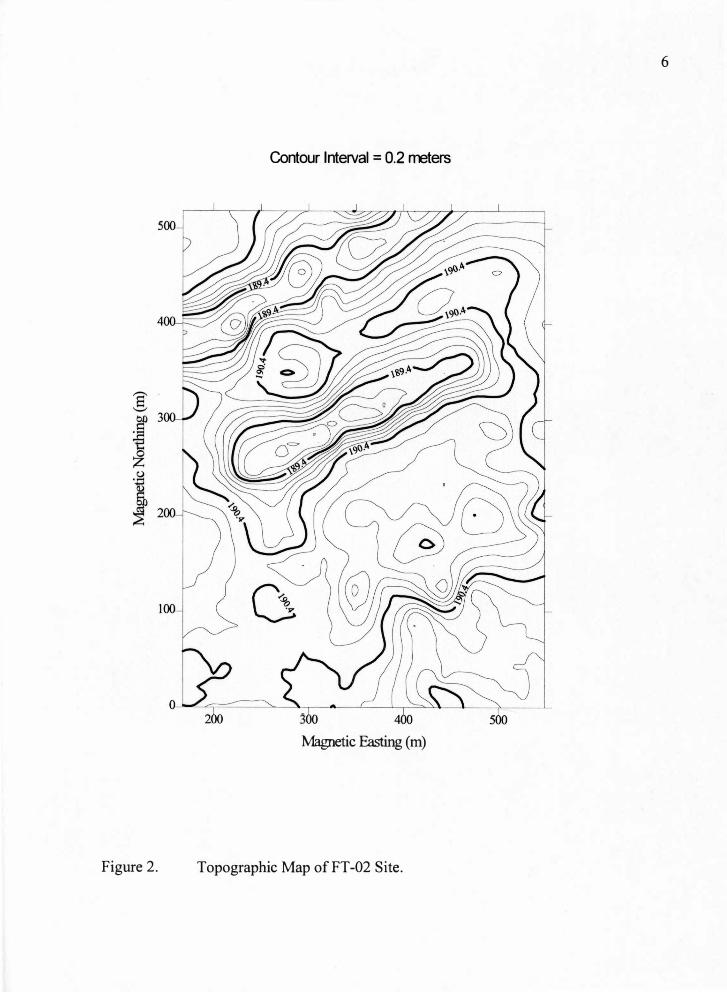
Changes in topography over the FT-02 site are very subdued, with elevations ranging

from 188 m to 192 m above mean sea level. Most of the topographic relief occurs in

two linear depressions that cross the middle of the site to the north and south of the

concrete fire pad and trend towards the east (Figure 2). The subsurface of the FT-02

site is comprised of glacial materials lying unconformably above the bedrock. The

glacial materials are composed of a flat lying glaciofluvial sand approximately 20 m

to 24 m thick and underlain by a 40 m to 76 m lacustrine silty clay. Depth to water

table in the unconfined aquifer of glaciofluvial sand ranges from 5 m to 7 m. The

direction of flow in the unconfined aquifer is from the northwest to the southeast, and

much of the flow discharges at the surface into the wetland complex located to the

south of the FT-02 site.

Site Geochemistry

Geochemical analyses of water samples have been run by NCIBRD on

samples from over 50 wells at the FT-02 site. The plume is comprised of several

distinct components (Figure 3). The JP-4 is comprised of aliphatic and aromatic

hydrocarbons, which exist either as a separate liquid phase above the ground water

5

6

Contour Interval = 0.2 meters

5

Magnetic Easting (m)

Figure 2. Topographic Map ofFT-02 Site.

�o 1'1E>ters

======= Grave/ Road

VArB

Q • �I.

0 0

0 0

0 0 0

0 0

0 0 0

0 0 0

FT-J◄ Mon;tor;ng w'el/ Loco t;on

Fig_ure 3.

0 1.2�

0 0

0 ••

.1�3.

0 0

0 0 0

. 3�6. 0 . 4?7•\\· 0

0 0 0 0 0 �\ 0

0 488

0 4 27

0 366

·305

0183

•0 122

PLUME0

0 0 0 0

0 0 0

Source:

FT-02 Site Plume With Well Locations.Modified fron, NCIBRD files. Used With permission ofM. Henry_

--

'-J

0

·o

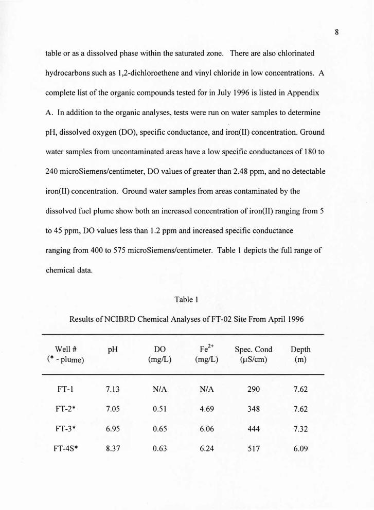
table or as a dissolved phase within the saturated zone. There are also chlorinated

hydrocarbons such as 1,2-dichloroethene and vinyl chloride in low concentrations. A

complete list of the organic compounds tested for in July 1996 is listed in Appendix

A. In addition to the organic analyses, tests were run on water samples to determine

pH, dissolved oxygen (DO), specific conductance, and iron(II) concentration. Ground

water samples from uncontaminated areas have a low specific conductances of 180 to

240 microSiemenslcentimeter, DO values of greater than 2.48 ppm, and no detectable

iron(II) concentration. Ground water samples from areas contaminated by the

dissolved fuel plume show both an increased concentration of iron(II) ranging from 5

to 45 ppm, DO values less than 1.2 ppm and increased specific conductance

ranging from 400 to 575 microSiemenslcentimeter. Table 1 depicts the full range of

chemical data.

Table 1

Results ofNCIBRD Chemical Analyses ofFT-02 Site From April 1996

Well# (* - plume)

FT-1

FT-2*

FT-3*

FT-4S*

pH

7.13

7.05

6.95

8.37

DO (mg/L)

NIA

0.51

0.65

0.63

Fe2+

(mg/L)

NIA

4.69

6.06

6.24

Spec. Cond (µSiem)

290

348

444

517

Depth (m)

7.62

7.62

7.32

6.09

8

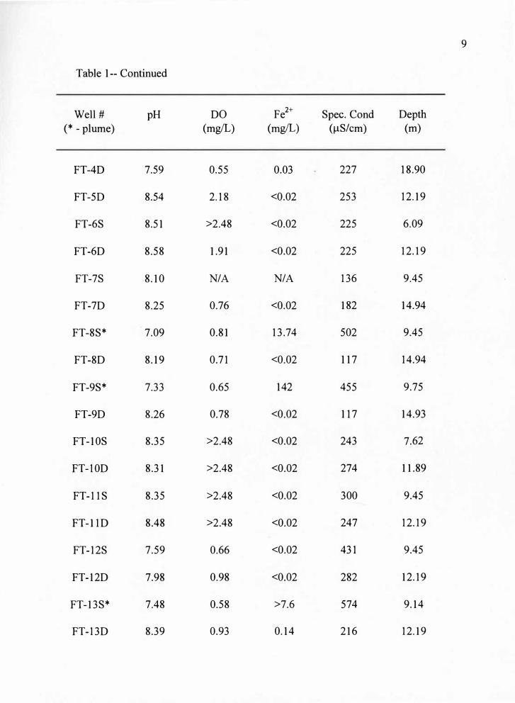
Table 1--Continued

Well# (* - plume)

FT-4D

FT-5D

FT-6S

FT-6D

FT-7S

FT-7D

FT-8S*

FT-8D

FT-9S*

FT-9D

FT-10S

FT-l0D

FT-11S

FT-1 lD

FT-12S

FT-12D

FT-13S*

FT-13D

pH

7.59

8.54

8.51

8.58

8.10

8.25

7.09

8.19

7.33

8.26

8.35

8.31

8.35

8.48

7.59

7.98

7.48

8.39

DO (mg/L)

0.55

2.18

>2.48

1.91

NIA

0.76

0.81

0.71

0.65

0.78

>2.48

>2.48

>2.48

>2.48

0.66

0.98

0.58

0.93

Fe2+

(mg/L)

0.03

<0.02

<0.02

<0.02

NIA

<0.02

13.74

<0.02

142

<0.02

<0.02

<0.02

<0.02

<0.02

<0.02

<0.02

>7.6

0.14

Spec.Cond (µSiem)

227

253

225

225

136

182

502

117

455

117

243

274

300

247

431

282

574

216

Depth (m)

18.90

12.19

6.09

12.19

9.45

14.94

9.45

14.94

9.75

14.93

7.62

11.89

9.45

12.19

9.45

12.19

9.14

12.19

9

Table 1 -- Continued

Well#

(* - plume)

FT-14S

FT-14D

pH

7.95

8.38

DO

(mg/L)

1.54

2.47

Fe2+

(mg/L)

<0.02

<0.02

Spec. Cond

(µSiem)

301

232

Depth (m)

9.45

12.50

Overall, the chemical data show that there is a decrease in specific

conductance with depth, as the deeper wells (denoted with a D) have lower values

than their shallow counterparts ( denoted with a S). All but one of the pH values is

above 7.0, indicating that neutral to slightly alkaline conditions are present throughout

the site. There appears to be a good correlation between increased conductivity and

iron(II) concentration in areas affected by the dissolved plume. Other ions species

concentration were unavailable.

10

CHAPTER II

REVIEW OF RELEVANT LITERATURE

Theoretical Models

Several models have been developed to describe fuel oil contamination with

respect to the hydrogeologic parameters and the electrical parameters. The

hydro geologic parameters help describe the shape and concentration of the plume

after the contaminant has entered the subsurface (Fetter, 1994). At this particular site,

FT-02, the contaminant is a light non-aqueous phase liquid (LNAPL) which mixes

with the ground water to a limited extent. Some of the JP-4 will reside directly above

the capillary fringe in a pool that is called "free product". This free product can

diffuse into the vadose zone, but will not diffuse into the saturated zone. A smaller

portion of the JP-4 can dissolve into the ground water in the saturated zone, where it

can be advected (carried along with the flowing ground water) and diffused

(spreading due to variability in flow paths in a porous matrix) further into the

saturated zone.

The 3-dimensional electrical properties of resistivity and electric permittivity

are highly variable between the vadose zone, the saturated zone and the contaminated

areas. Resistivity is defined as the inverse of the ability to transmit current; materials

11

with a high resistivity require more potential to transmit a given amount of current

than materials with a low resistivity (Telford and others, 1990). The bulk resistivity

of a granular rock or unconsolidated sediment can be modeled by the parameters of

porosity, fluid resistivity, degree of saturation and a cementation factor by using

Archie's Law (Archie, 1942). Archie's law is an empirical relationship that links the

various parameters to the bulk resistivity. Soil and glacial material can be modeled

by

where Pb is the bulk resistivity; a, m, and n are empirically derived constants; S is the

fraction of the pores containing the fluid, and Pf is the fluid resistivity. The bulk

resistivity of a soil is highly dependent on the resistivity and degree of saturation of

the fluids in the pore spaces. The resistivity of the matrix materials ranges from

4E+10 Ohm-meters for pure quartz to 20 Ohm-meters for an unconsolidated wet clay

(Telford and others, 1990). Theoretical models by Endres and Redman (1993)

demonstrate that as hydrocarbon saturation in porous media increases, the bulk

resistivity increases as well. Endres and Redman (1993) also demonstrated that the

relative electrical permittivity can change from 20 for a mixture of uncontaminated

ground water and sand, to 4 for a mixture of petroleum hydrocarbons and sand.

A survey of the properties ofLNAPLs by Monier-Williams (1995)

summarizes some possible mechanisms for an increase in resistivity and some

12

,1,.•ms•n Pb== a'!' Pf

possible mechanisms for a decrease in resistivity of a LNAPL plume. The

mechanisms for an increase in resistivity involve the dynamic displacement of the

water by the LNAPL resulting in depletion of the aqueous phase, a loss of the

capillary fringe and depression of the water table, reduction in connectivity of the

aqueous phase, and a change in the wetting phase of the aquifer solids (Monier­

Williams, 1995). The mechanisms for a decrease in resistivity involve alternate

changes in the wetting phase of the aquifer solids, the formation of emulsions

increasing the water/LNAPL surface contact area, enhanced aqueous phase

connectivity due to changes in the gas phase, and additives in the original LNAPL that

would enhance current flow (Monier-Williams, 1995)

Controlled Spill Studies

Several experiments have been undertaken in the laboratory in order to test the

hypotheses developed from the theoretical models. These experiments were run in a

tank or column constructed to model a glacial aquifer. Typically, a model was

injected with a known amount of hydrocarbons, and monitored with geophysical and

geochemical analyses over time to see what the effect of injection would be. A tank

model developed by DeRyck and others (1993) showed a strong increase in resistivity

in the capillary fringe as the hydrocarbon (kerosene) displaced the water in a portion

of the capillary fringe.

A column experiment by Gajdos and Kral (1995) indicated that at low

concentrations of hydrocarbons (less than 5% by liquid phase volume), a decrease in

13

resistivity in the saturated zone can be measured of up to 20% of the original bulk

resistivity. This decrease was attributed to a non-equilibrium state in the wetting

phase that preferentially channelled current through the pores. The authors noted an

increase in resistivity as concentrations increased past ten percent of the starting

volume.

A tank experiment by Grumman and Daniels (1995) simulated a kerosene spill

in a sand matrix in order to test the electrical behavior by adding the kerosene into

ports that connected with the aquifer. The electrical properties were measured

indirectly with a ground penetrating radar (GPR) unit, and demonstrated that a GPR

signal can be attenuated slightly by the presence of kerosene in the vadose zone and

the capillary fringe. This is attributed to either a redistribution of soil moisture or

contaminant vapor effects (Grumman and Daniels, 1995).

The results of the controlled spill studies show that the apparent resistivity

increases as the kerosene or other light hydrocarbon displaces the water in the

capillary fringe and in the water table below. Occasionally, a decrease in resistivity is

measured, which has been attributed to current channeling due to a change in the

wetting phase of the grains. This change involves replacement of water by LNAPL as

the wetting fluid on the grain surface. This will restrict the water to the middle of the

pore space, and the effective cross section of the water in the pore space is reduced as

well. This reduction in cross section will allow current to pass easily through a layer

that appears to be mostly hydrocarbon. As the hydrocarbon concentration increases in

14

the pores, this decrease in resistivity declines and then switches back to an increase in

resisitivity.

Field Studies

Several field studies have been conducted over known hydrocarbon

contamination plumes to test whether the phenomena observed in the laboratory

studies can be duplicated by actual spills. The field studies range in age from less

than 1 week, to some more than 10 years.

Daniels and Vendl (1992) found a decrease in GPR amplitude which they

interpreted as being due to the contaminant vapor phase in the capillary fringe. The

study found a correlation between the decrease of the GPR signal amplitude in the

vicinity of the gasoline concentration and the presence of gasoline. The decrease in

amplitude was determined to be located in the vadose zone, and is attributed to the

contaminant vapor phase.

Mazac and others (1990) found that a very young (less than 1 week) spill had

a high electrical resistivity in contaminated areas. The survey was conducted in

Quaternary sands and gravels, with a free product plume 0.2 m thick. Vertical

electrical soundings (VES) and a modified mise-a-la-masse (MALM) survey were

used to measure the electrical resistivity over the contamination. The high electrical

resistivity was attributed to the insulating properties of the fuel oil contaminant.

A case history by Maxwell and Schmok (1995) shows an anomalous region of

decreased GPR amplitude over a hydrocarbon plume, but based their depth estimate

15

of the plume on fully saturated conditions. This is contradictory to their assertion that

the decreased GPR amplitude is due to the contaminant vapor phase, which would be

located in the vadose zone. Also, the anomalous GPR amplitude has a signature that

is more indicative of conductive surficial fill in a trench.

A case history by Monier-Williams ( 1995) found low electrical resistivity in

areas with significant free product thickness around a landfill. The low electrical

resistivity was measured with a frequency domain electromagnetic induction

instrument. The reason for the low electrical resistivity was attributed to either an

emulsion or enhanced surface conductance at the fuel oil-aqueous contact. A good

statistical correlation between maximum free product thickness and low electrical

resistivity was seen, however, no chemical basis for the theorized emulsion was

shown.

A similar case history by Gajdos and Kral (1995) also measured a low

electrical resistivity over areas associated with fuel oil pollution. The low electrical

resistivity was measured with a frequency domain electromagnetic induction

instrument. The low resistivity was attributed to the increase of free ion density due

to a change in the wetting phase.

A study of a gas station tank leak by Grumman and Daniels (1995) found GPR

signal attenuation in areas of hydrocarbon contamination above the interpreted water

table. The site cover is glacio-lacustrine soil, with strong contaminant vapors present

in the vadose zone. The GPR signal attenuation is attributed to the contaminant vapor

phase in the vadose zone causing loss of signal.

16

There are three classes of results from the field studies. First, electrical

resistivity highs are measured over very young spills in the capillary fringe. Second, a

decrease in GPR amplitude can be measured over contaminated areas in either the

capillary fringe or in the saturated zone. Third, low electrical resistivity is measured

in contaminated areas that are of an older age.

Geochemical Studies

There are several papers dealing with the geochemistry of a hydrocarbon

contamination plume. A series of papers was based on analyses of a pipeline spill

near Bemidji, Minnesota. The spill was monitored over time to see how the plume

evolved chemically. The first paper, by Bennett and others (1993), discussed how the

dissolved portion of the hydrocarbon plume was degraded naturally by microbes

present in the soil. This degradation, also known as natural bioattenuation, showed

that several distinct chemical zones developed in the regions down gradient and

within the dissolved plume. These zones were dependent on the specific

electrochemical makeup of the ground water, and followed a regular pattern (Bennett

and others, 1993).

The second paper, by Eganhouse and others (1993), discussed the amount and

type of hydrocarbons present in each zone. In addition, the authors established the

particular type of hydrocarbon that was most likely to degrade in each zone. All types

of hydrocarbons were found to degrade in oxic zones, but the rates varied

17

significantly (Eganhouse and others, 1993). Overall, the results of the second paper

supported the degradation zones established by the authors of the first paper.

The third paper, by Baedecker and others (1993), dealt with the specific

reactions that occur in each zone that lead to the degradation of the hydrocarbon. The

products of the bioremediation include: soluble iron(II) and manganese(II),

production of organic acids in anoxic zones, CO2 and CH4 (Baedecker and others,

1993 ). The presence of CO2 and organic acids can lower the pH of the ground water,

and bring more ions into solution (Bennett and others 1993). In addition to the

chemical studies, physical measurements on the fluid resistivities of uncontaminated

and contaminated regions of the dissolved plume at Bemidji have shown a 3 to 5 fold

decrease in resistivity when comparing ground waters from contaminated regions to

uncontaminated regions.

The fourth and final paper, by Cozzarelli and others (1994), discussed the

evolution of organic acids from the degradation of the hydrocarbon. The authors

concluded that location of the production of organic acids varied over time, as the

chemical zones shifted location. Organic acids were found to accumulate in anoxic

groundwater, and when oxygen is present, the acids are degraded as well.

The conclusion of the geochemical literature is that hydrocarbons will degrade

over time, if the terminal electron acceptors ( oxygen, nitrate, ferric iron and others)

are present. These degradation reactions will evolve CO2 and will increase the

acidity of the ground water. This increase in acidity can aid in the dissolution of

aquifer solids, which will increase the ionic content of the ground water. The end

18

result of these reactions can bring about a decrease in apparent resistivity. This is in

disagreement with the earlier intuitive geophysical models, which theorize that

electrical resistivity increases over hydrocarbon contamination, but does provide a

plausible explanation for why many field studies have shown decreased electrical

resistivity over hydrocarbon contaminated sites around the dissolved plume.

19

CHAPTER III

METHODOLOGY

Self Potential

The self potential (SP) method was developed in mining exploration, and also

applied to well logging for petroleum exploration (Telford and others, 1990). There

have been several attempts at applying the SP method to water resource evaluation,

with varying degrees of success (Corwin, 1990). The self potential is a natural

potential present beneath the Earth's surface that is generated by several physical and

chemical mechanisms. The mechanisms that can cause the self potential are: the

streaming potential, the diffusion potential, the Nemst potential, and the electrolytic

contact potential (Telford and others, 1990). An in-depth analysis of the various

mechanisms that comprise the self potential can be found in Telford and others (1990)

or Corwin (1990). Although it is nearly impossible to determine the amount each self

potential mechanism adds to the self potential, qualitative estimates of the

contribution by each mechanism can be evaluated based on the geologic conditions at

a particular site.

The data were acquired using non-polarizing electrodes and a high input

impedance voltmeter. The non-polarizing electrodes consisted of a PVC housing and

a porous plug (a wooden dowel) in contact with a saturated solution of copper sulfate.

20

This solution was placed in contact with a copper wire to act as an electrode, with the

copper sulfate solution making the connection between the subsurface and the

voltmeter. The use of the non-polarizing electrodes allowed for the exclusion of

electrolytic contact potentials at the metallic electrodes. The high input impedance

voltmeter was used so that the measurement of potentials between two electrodes

would not be interfered with by current leakage through the voltmeter.

The survey was conducted over the southern portion of the site utilizing a

fixed reference electrode at 305 m North and 472 m East. Potentials were measured

at 15.24 m intervals along east-west lines, and the mobile electrode was returned to

the reference electrode position to measure drift after 4 east-west lines had been

surveyed. The data were plotted in SURFER, using the kriging option for generating

the contour plot.

Mise-a-la-masse

The mise-a-la-masse (MALM) method was developed in the mining industry

in order to roughly determine the boundaries of an ore body after one borehole had

been drilled into a conductive sulfide mineral deposit. The method makes use of a 4

electrode system, 2 current electrodes and 2 potential electrodes. One current

electrode is placed down the borehole into the ore body, and the other current

electrode is placed very far away from the borehole on the ground surface (Figure 4).

One of the potential electrodes is placed on the ground surface very far away from

21

B@ CO·�'------,L

Figure 4.

A M N B

t J l t-�tlW I�

�---A�---

Dif

,o\t - D,pole. R.es 1s+;0i+y Pro911, tlj A ·e M N

+ i l t.I I <'-- (l - ->!.---(\a_---:,;<:--<.\.-') : I

Electrode Configurations for Mise-a-la-masse, Vertical Electrical

Soudings, and Dipole-Dipole Resistivity Profiling.

22

either the downhole or surface current electrodes. The other potential electrode is

used to measure the potential difference on the surface around the borehole electrode.

It can be demonstrated from electrical theory that the potential around the downhole

electrode will appear as a radially concentric pattern, with the largest potential

difference located near the downhole electrode (Telford and others, 1990). This

radially concentric pattern will only appear in a homogenous subsurface with no

variations in the electrical resistivity. In the presence of a conductive ore body, or

conductive contaminant plume, the radially concentric pattern will distort to roughly

follow the boundaries of the conductive body (Telford and others, 1990). This is due

to the increased density of current in the conductive region, which leads to a higher

potential difference relative to the distant potential electrode. The conductive

subsurface body acts as an extended electrode of constant potential.

In this study, for lack of a better access point to the plume, the "downhole"

current electrode was attached to the steel casing of the cable tool drilled well FT-4D

located at 311 m North, 309 m East. The surface return current electrode was placed

at 335 m North, 76 m East and the surface potential reference electrode was placed at

274 m North, 503 m East. The potential drop was measured using the BISON 2390

resistivity meter, which used a constant current source of 100 mA, allowing all

potentials to be plotted without normalization. The potential differences were

corrected for the minor influences of the distant surface current and potential the

electrodes not being located at infinity, and were contoured using the kriging option

23

on SURFER.

Electrical Resistivity

Vertical Electrical Soundin� (VES)

Vertical electrical sounding is a resistivity measurement using a four electrode

system similar to the one described in the mise-a-la-masse section. In this case, all

four electrodes are located in a line on the surface. The two current electrodes are

placed outside of the two potential electrodes. In Figure 4, the current electrodes are

labeled A and B, with AB equal to the distance between the current electrodes. The

potential electrodes are labeled M and N, with MN equal to the distance between the

potential electrodes. An expression can be used to calculate the apparent resistivity of

the earth based on the input current, measured potential difference, and the surface

geometry of the electrodes by the equation:

Pa = (1t/4) * [ ((AB)2 - (MN)2)/(MN)] * (VII)

where V = potential difference in Volts, I = input current in Amperes and Pa =

apparent resistivity in Ohm-meters.

Apparent resistivity is a field measured quantity that gives relative information

about the resistance to current flow in a particular volume of the subsurface (Telford

�d others, 1990). In the case of a homogeneous isotropic earth, the apparent

resistivity will remain constant for all electrode configurations, and over any range of

24

input currents. By measuring the changes in terms of apparent resistivity, it is

possible to infer vertical and lateral changes in electrical resistivity over a particular

area. The VES method determines the change in apparent resistivity with depth, by

expanding the current electrode spacing AB and keeping the potential electrode

spacing MN constant around a fixed center. The data are plotted on a log-log graph

with apparent resistivity on the vertical axis and AB/2 on the horizontal axis. The

apparent resistivity curve was inverted in an iterative I-dimensional computer

program which finds the best statistical fit to a measured field curve starting with an

operator-supplied resistivity versus depth model. There is a great deal of uncertainty

in the results, due to the Principle of Equivalence, as a layer of a given thickness and

resistivity can be modeled as a thicker and less resistive layer to give the same effect

on a maximum portion of a VES curve and the expression of thickness divided by

resistivity is constant for the minima of the VES curve (Telford and others, 1990).

However, by matching the resistivity layer thicknesses to known geological controls

such as topsoil, vadose zone, and saturated zone thickness at a control well, a good

estimate of the true resistivity of layers and thicknesses elsewhere can be determined.

For this study, several model resistivity values were calculated to estimate the effect

of the Principle of Equivalence and the Principle of Suppression.

Three soundings were measured over the FT-02 site, each using six steps per

decade of AB/2, and stopping at AB/2 = 100 meters. VES # 1 was measured 259 m

North, 351 m East; VES # 2 was measured at152 m North, 396 m East; and VES # 3

25

was measured at 107 m North, 448 m East. VES # 1 located within the dissolved

plume, used the BISON 2390 resistivity meter. VES # 2 located on the border of the

dissolved plume, used the SYSCAL R-2 resistivity meter. VES # 3 located outside of

the boundaries of the dissolved plume, used the SYSCAL R-2 resistivity meter.

Dipole-Dipole Resistivity Profilin2

Dipole-Dipole resistivity profiling (DDR) is another in-line resistivity

measurement like the VES method. The DDR method combines elements of

profiling, the measurement of lateral changes in apparent resistivity, and sounding, the

measurement of vertical changes in apparent resistivity. In the field array the

potential electrodes are closely spaced and remote from the current electrodes, which

are also closely spaced (Telford and others, 1990). The close spacing between the

pairs of the current and the potential electrodes is held constant, and the separation

between these dipoles is an integer multiple of the constant spacing. A general

schematic of the field layout is shown in Figure 4, with the equation for the apparent

resistivity given by:

Pa= 7t *a* n * (n+l) * (n+2) * (VII)

where a = electrode dipole spacing in meters , n = integer spacing in meters, V =

potential difference in Volts, I = input current in Amperes, and Pa = apparent

resistivity in Ohm-meters. The data were collected at regularly spaced intervals by

26

holding the centerpoint between the groups fixed and expanding the distance between

the groups out to n=4. The centerpoint was then shifted along the line by the "a"

spacing and the dipole separation was again expanded from n= l to 4. After all the

data have been collected and all the apparent resistivities calculated, the data are

presented in a pseudosection format as described in Telford and others (1990).

Three dipole-dipole surveys were measured over the FT-02 site. The first

survey was collected along line 305 m North with 10 meter dipole spacings using the

SYSCAL R-2 resistivity meter. The second survey was collected along line 274 m

North with 15 meter dipole spacings using the SYSCAL R-2 resistivity meter. The

third survey was collected along line 305 m North with 20 meter dipole spacings

using the SYSCAL R-2 resistivity meter.

This pseudosection apparent resistivity data are then inverted using an

iterative 2-dimensional computer program which generates theoretical earth models

that would give the measured pseudosection values. The particular program used in

this study was RES2DINV, a quasi-Newton solving method designed to invert

measured DDR profile data into a theoretical earth model (Loke and Barker, 1995).

As in the VES computer inversions, there is a great deal of uncertainty in the results,

again due to the Principle of Equivalence. This uncertainty is present both in the

vertical and lateral positions of the apparent resistivity structures, as they are

determined from the apparent resistivity parameter. The apparent resistivity

parameter is simply a ratio that reflects the effect of potential drop, current, and the

27

/

geometry of an array (Telford and others, 1990), and is not simply related to the true

resistivity structures which lie beneath the surface. For this site, the inverse model

resistivity depths from this program for the various "n" values were divided by two in

order to better fit known depth to a principal resistivity boundary, the vadose zone -

saturated zone interface. In addition to the inverse models, 2 forward models were

developed in order to estimate the effects of the water saturated zone and the clay

layer have on the measured resistivity pseudosection.

Electromagnetic Induction

The electromagnetic induction method was originally developed for the

detection of conductive ore bodies in the mining industry. There are two major types

of electromagnetic induction equipment, frequency domain and time domain. The

two instruments used in this study are frequency domain units. The theory of

electromagnetic induction can be found in many texts, such as Telford and others

(1990) or Dobrin and Savit (1990). The underlying principle of frequency domain

electromagnetic induction is as follows. A primary electromagnetic (EM) signal of

constant frequency and power is sent out from a transmitter coil. This primary EM

signal travels into the subsurface and interacts with conductors that are present. The

interaction of the primary EM signal and the subsurface conductors induce a circular

current flow in the subsurface conductor. This "eddy" current flow, in turn, creates a

secondary EM signal. The secondary EM signal, along with the primary EM signal

28

that travels through the air, is measured at a receiver coil. The secondary signal

properties are dependent on the electrical resistivity, relative electrical permittivity,

and the magnetic permeability of the subsurface. Since the operating frequency of the

measurements is low with respect to the electromagnetic spectrum, the relative

permittivity has an insignificant effect on the secondary signal (McNeill, 1980). The

relationship between the primary and secondary signal is expressed as the amount of

secondary in-phase with the primary, and the amount of signal 90 degrees out-of­

phase from the primary is measured as well. The out-of-phase ratio can then be

converted into an apparent conductivity, using the assumptions developed by McNeill

(1980). This apparent conductivity shares the same characteristics as the apparent

resistivity parameter discussed previously, as the apparent conductivity is the inverse

of the apparent resistivity.

The two units used in this study were the Geonics EM-31 and EM-34. Both

were employed in the horizontal loop configuration, which provided the maximum

depth penetration of which the unit is capable of (McN eill, 1980). The EM-31 data

were collected along numerous EW and NS trending lines, while the EM-34 data

were collected along several EW trending lines only using the 20 meter coil spacing.

In addition, forward models were run on a generalized resistivity structure to estimate

the expected values of ground conductivity off and on the plume.

29

.

Ground Penetrating Radar

The principles and theory of GPR are based on the wave equation which is

derived from Maxwell's equations, a succinct summary of which can be found in

Daniels (1989). The parameters that affect GPR are co�ductivity (cr), magnetic

permeability(µ), and electric permittivity (t). The paramter of magnetic permeability

was not considered in this study because the concentration very low in common earth

materials. The two properties that affect attenuation and propagation of

electromagnetic waves are cr and t (Daniels, 1989). The velocity of the GPR signal is

approximated by:

where V m = velocity in the medium in meters per second, V c

= velocity of light in a

vacuum (3 E+08 mis), tr= relative electrical permittivity, which is unitless. The

attenuation of the GPR signal is governed both by tr and cr, with the cr term

dominating the attenuation factor at cr = 5.6 mS/m or greater for a 100 MHz radar

signal in a saturated aquifer (tr= 20) (Daniels, 1989).

GPR data were collected along north-south and east-west lines, with 30.5

meters between lines. The gain function of the amplifier was set in an area known to

be free of contamination and set such that later signals had approximately the same

amplitude as the early signals. Bistatic 100 MHz antennae were used with the GSSI

30

SIR-10 GPR system. The scan length of all records was 400 nanoseconds, with a

sample digitization rate of 512 samples/scan. Scans were generated at 40

scans/second. Acquisition filters used were 3-stage Instantaneous Impulse Response

(IIR) with low-pass set at 80 cycles/scan and high-pass at 10 cycles/scan. Horizontal

smoothing was accomplished with a 5-scan running average filter. Field data were

down loaded to a personal computer for data processing.

Data processing consisted of rectifying the horizontal scale to approximately

15 scans/meter to account for variances in the towing speed of the antennae. GPR

lines were also corrected for changes in topography by applying static shifts based on

ground elevation. No post-processing filters were applied to this data set.

31

CHAPTER IV

RESULTS

Self Potential

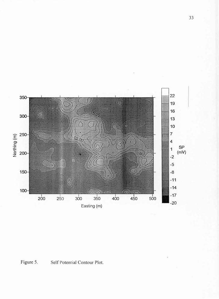
The drift corrected data from the self potential survey were plotted and

contoured in SURFER, utilizing the kriging option to interpolate values between

measured points. The data are presented in Figure 5. There is high positive trend

passing through the center of the surveyed region, oriented around N 30 W. The

positive trend has a value ranging from 10 to 20 mV, with background values in the

region ranging around -5 mV to +5 mV. There is a secondary positive trend to the

east of the major trend, with a value ranging from 10 to 16 m V.

Mise-a-la-masse

The normalized potential data from the mise-a-la-masse survey were plotted

and contoured in SURFER, utilizing the kriging option to interpolate values between

the measured points. The map results of the raw and processed data are presented in

Figure 6. There is an circular trend passing through the surveyed area, with higher

potential differences nearest to the location of the downhole current electrode, and the

lowest potential differences furthest from the downhole current electrode. There is

slight deviation from the circular trend around the point 260 m North 411 m East

32

,-... 2

0 2 z

1

1

200 250 300 350

Easting (m)

Figure 5. Self Potential Contour Plot.

400 450 500

22

19

4

1

-2

-5

-8

-11

-14

-17

-20

33

SP (mV)

E .._, O> C

€

34

MALM Field Data - Contour Interval 10 mV

fvlagnetic Easting (m)

MALM Processed Data - Contour Interval 4 mV

fvlagnetic Easting (m)

Figure 6. Mise-a-la-masse Contour Plots.

Mag

netic

Nor

thing

(m)

Mag

netic

Nor

thing

(m)

oo·o

0 8

that has a lower negative potential than the circular trend.

Electrical Resistivity

Vertical Electrical Soundin�

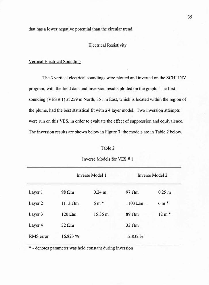
The 3 vertical electrical soundings were plotted and inverted on the SCHLINV

program, with the field data and inversion results plotted on the graph. The first

sounding (VES # 1) at 259 m North, 351 m East, which is located within the region of

the plume, had the best statistical fit with a 4 layer model. Two inversion attempts

were run on this VES, in order to evaluate the effect of suppression and equivalence.

The inversion results are shown below in Figure 7, the models are in Table 2 below.

Table 2

Inverse Models for VES # 1

Inverse Model 1 Inverse Model 2

Layer 1 98nm 0.24m 97 nm 0.25 m

Layer 2 1113 nm 6m* 1103 nm 6m*

Layer 3 120nm 15.36 m 89nm 12 m *

Layer 4 32nm 33nm

RMS error 16.823 % 12.832 %

* - denotes parameter was held constant during inversion

35

-

E

E

� ·5

c � ro

Figure 7.

1000

� � 0

100

0

□

6

1

0

0 0 � ij

�

Curve

Field Data

Inverse Model 1

Inverse Model 2

10

AB/2 (m)

Field and Inverse Model Plot for VES # 1.

36

§

D

D 0

0 6

@

100

10

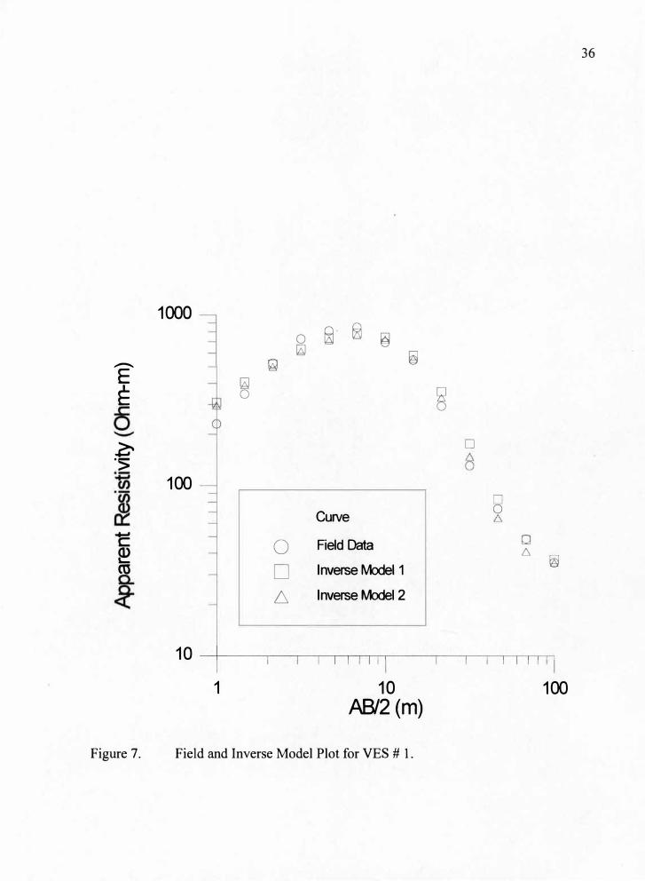
The second sounding (VES # 2) at 152 m North, 396 m East, which is located on the

border of the plume, had the best statistical fit with a 5 layer model. Due to the

extreme decrease in resistivity with depth, no forward models were attempted on this

model. The resultant inverse model is shown below, the plot of field and model

values are on Figure 8 with the inverse model shown below in Table 3.

Table 3

Inverse Model for VES #2

Inverse Model

Layer 1 3632 nm 0.14 m

Layer 2 33000 nm 0.89 m

Layer 3 5600 nm 7.27 m

Layer 4 800nm 10.0 m *

Layer 5 27nm

RMS error 11.223 %

* - denotes parameter was held constant during inversion

The third sounding (VES # 3) at 107 m North, 488 m East, which is located in an area

well outside of the plume, had the best statistical fit with a 5 layer model. In addition

to the inverse model, two forward models were run in order to evaluate the effects of

equivalence and suppression on layer 4. The models are shown below, and plots of

37

38

100000

10000 0 8 0 □ �

8 §---�

0

·5

1000

.... Curve C

8 � □ Field Dataro 100

0 Inverse Model

8

10

1 10 100

AB/2 (m)

Figure 8. Field and Inverse Model Plot for VES # 2.

-E E

• 1n B

0

the field and model resistivities are shown in Figure 9 and the inverse and forward

models are shown in Table 4.

Table 4

Inverse and Forward Models for VES # 3

Apparent Resistivity and Thickness of Layer

Inverse Model Forward Model 1 Forward Model 2

Layer 1 3631 nm 0.1 m* 3632 nm 0.14m 3632 nm 0.14m

Layer 2 33086 nm 1.14 m 33000 nm 0.89m 33000 nm 0.89m

Layer 3 6970 nm 6.84m 5600 nm 7.27 m 5600 nm 7.27m

Layer 4 4200nm 3.67m 400nm 10.0m 1600 nm 10.0m

Layer 5 42nm 27nm 27nm

RMS 6.27 % NIA NIA

error

* - denotes parameter was held constant during inversion

Dipole-Dipole Resistivity Profilin2

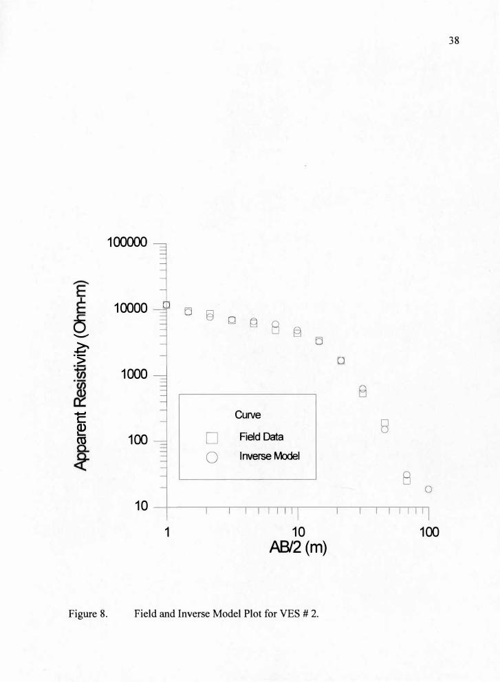
Three dipole-dipole resistivity soundings were deployed across the plume . The

first and second profiles were extended along line 305 m North . The first profile,

measured with a 10 meter dipole, is shown in Figure 10 along with the associated

inverse model, and the tabular data for the field data are in Appendix B. In Figure 10,

39

40

100000

Qi � li]

E 10000 �

8 e

� � ">

1000 6.

� Curve �

0

◊ Field Data 6.

□ Inverse l\t1odel 8co 100 0 Forward fvlodel 1 6.

� 6 Forward�2 8

10

1 10 100

AB/2 (m)

Figure 9. Field and Inverse Model Plots for VES # 3.

E

-

188

n

2

3

4

Depth 188

0.9

2.6

4.4

meters

6.4

0.5

228 268

Eosting nlong line 305 m North 308 348 388 428 468

Dipole Length= 10.0 meters

RMS error = 2.410

m.

-I

228 268 308 348 388 428 468 m.

c=J C=:J c::=J EiIJl 1-·-·-·-•.-4 mml mm mim l:liil.W 11111111 -123 ?35 451

hwerse Model nesisliuily Section

Ofifi 1661 0hm-mP.tcrs

Figure 10. Dipole-Dipole Resisitivity Profile Along Line 305 m North, 10 m Dipoles.

Field Data

there is an overall decrease in resistivity with depth with values ranging from 1600

nm to 2500 nm at the first datum level down to 100 nm and less at the fourth datum

level. Superimposed on top of this sharp decrease in resistivity with depth is a lateral

decrease in resistivity. The decrease occurs in 3 symmetrical peaks, with the center of

the middle peak around 318 m East. Overall, the 3 peaks are spread out from 288 m

East to 348 m East, and appear to be measurable at the first datum level in the field

pseudosection.

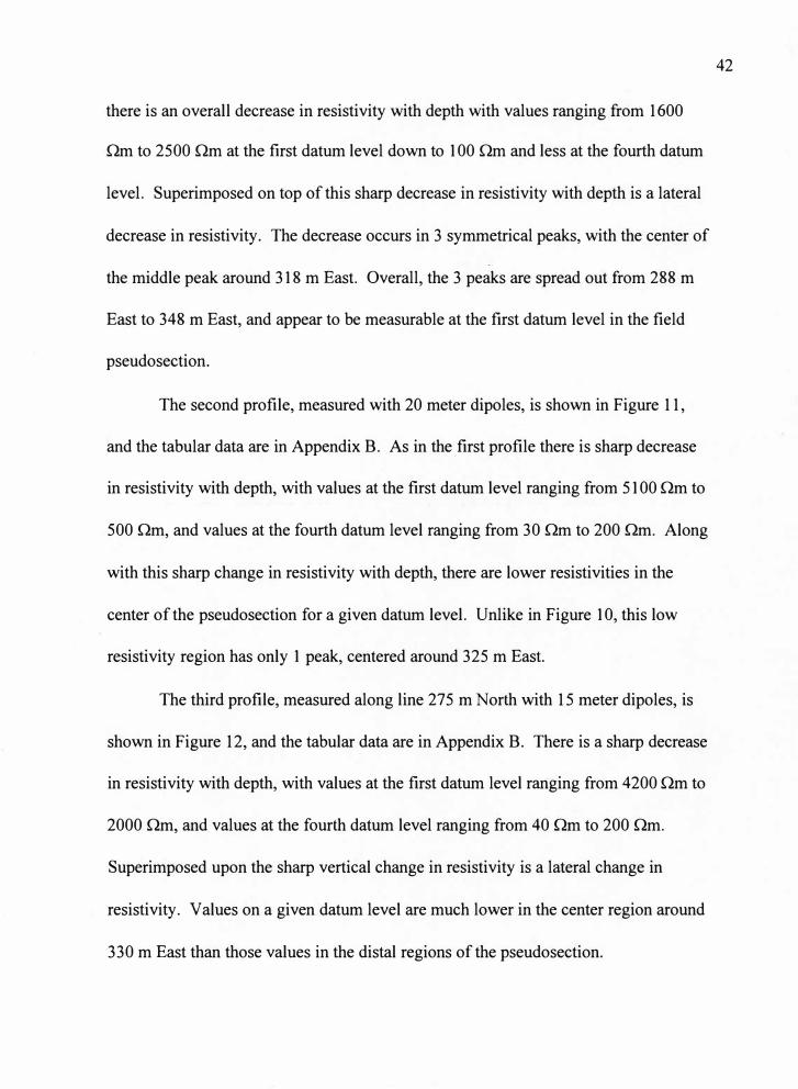
The second profile, measured with 20 meter dipoles, is shown in Figure 11,

and the tabular data are in Appendix B. As in the first profile there is sharp decrease

in resistivity with depth, with values at the first datum level ranging from 5100 nm to

500 nm, and values at the fourth datum level ranging from 30 nm to 200 nm. Along

with this sharp change in resistivity with depth, there are lower resistivities in the

center of the pseudosection for a given datum level. Unlike in Figure 10, this low

resistivity region has only 1 peak, centered around 325 m East.

The third profile, measured along line 275 m North with 15 meter dipoles, is

shown in Figure 12, and the tabular data are in Appendix B. There is a sharp decrease

in resistivity with depth, with values at the first datum level ranging from 4200 nm to

2000 nm, and values at the fourth datum level ranging from 40 nm to 200 nm.

Superimposed upon the sharp vertical change in resistivity is a lateral change in

resistivity. Values on a given datum level are much lower in the center region around

330 m East than those values in the distal regions of the pseudosection.

42

1.'l.'l

n

2

3

1

Depth 133

1.7

S.2

8.7

meters

12.7

17.0

21.'l Easling along line .'l05 m Nocth

293 .'l7.'l

. ii.I H: H: U IHI::: Ii! IJ}!.j;->>�·J5>·�sc�.[f Ii Ii Ii rf_�:.:�;�\�>-�-�,ij Hi:: iii i ifffiTfllii I ii I it, l: :,1 J.11 !,.I l.l,IJ..111(�•.l):-))):•:❖:-:•>fli' f

l I I I I I I I I I l I I I lip-(':•:•:-:-:-:-:-� .. 111111111111111 I fl 1111111

-it·�:1n�?'?�-?�\�:r�rtnff}rr{fi'"fi'"i111:.11: 1 u.1 t I � 1� 1i111 :n-� .. ;i•;=-

r���f�:�gtggff½tsr-, 1 !I !l ! lll!l In I !I (1/lili I! I! l!l !l l l!JJJlU !l!I. t :·.::::::.::::: :-,J_.q: t:J l ! :! J!: f IJ nr1�nrirrqrir

_'�� � :·� :� :� :': :� '.��JJ}J_ll)J_J.J_J)_J..i_�:� :� :�:::::: :·�:::::::::::::::::::::: . : :):':1t�� �'='}J_lJ)J)1)J)J)1) 1

. . . . . . . . . . . . . . . . . . . . . . .

·:��HHlHHfi!f=•·:::�.-

· · · · · · · ·.·.·.·.:.·.·.·.·.·.·.·.·.·: :·· Field Doto Dipole Lengt11 = 28 meters

213

RMS error = 7.8% 293 373

45.'l m .

'153 m.

c:::J c:::J G:=J [!lill) � !!!!!] - IBH8 llm!il - -17.1 152 189 1571 5017 Ohm-meters

lnuene Model Resistiuity Section

Figure 11. Dipole-Dipole Resisitivity Profile Along Line 305 m North, 20 m Dipoles. +:>, w

' / lXQ#IQ,X

\·•:•·•:•·········::::::,::i:i:i~::;:,._:,.:;:;:;:;:_·~·:: :::::::::.·:, ;,::) <,>.,:.>.:,::,::_::,:~:~:/

202

n

2

3

4

Depth 202

1.3

3.9

6.6 meters

9.5

12.0

262

262

[osllng olong line 274 m North 322

RMS Error = 14.3'1.

322

� C=:J c:=J Dill Ez:l I"""' mm! CBBB � 11Z1Z11 -

182

382

7.2 33.1 151 600 3139 Ohm-meters

lni•er\e Model Resi�tiuilu Section

442 IT'.

442 m.

Figure 12. Dipole-Dipole Resisitivity Profile Along Line 275 m North, 15 m Dipoles. .l:,. .l:,.

Field Oata Oipole Length = 15.0 metcn

Overall, each resistivity pseudosection shows a sharp decrease in resistivity

with depth. Along with this sharp vertical change, each pseudosection shows lower

resistivity values in the center region along a given datum level. The apparent

resistivity values change from survey to survey, but generally values on the first

datum level range in 1 000s of nm and values on the fourth datum level typically

range in the 1 Os of nm to the 1 00s of nm.

Electromagnetic Induction

The EM-31 and EM-34 profiles along Line 305 m North are shown in Figure

13. The coincident EM-31 and EM-34 profiles for several other lines are shown in

Appendix B. In the EM-34 profile there are two major spike anomalies near the ends

of the profile, with a minor drop in apparent conductivity around 325 m East. The

EM-31 profile shows several spike anomalies at the western edge of the profile, and a

slight high in apparent conductivity centered around 350 m East. There are no spike

anomalies at the eastern edge of the EM-31 profile. A line by line comparison of the

spike anomalies revealed several linear trends over the FT-02 site.

Ground Penetrating Radar

The GPR profile for line 305 m North is shown in Figure 14. The line for 305

m North shows a strong reflection doublet at approximately 80 nanoseconds into the

record. The amplitude of the record below the doublet around 80 nanoseconds varies

45

-. 40 E

� --

� ·5

g 0 "'O C

8 C

-�Q)� -40

-. 40 E

� --

� ·5

g 0 "'O C

8 C

-�

EM-34

EM-31

Q)� -40___._-----,---------,-----r-------.--

200 400 Easting (m)

Figure 13. EM-31 and EM-34 Profiles Along Line 305 m North.

46

w

200

300

Figure 14.

Legend:

IS

A

ISA

,� 321

Shadow Zone

GPR Profile Along Line 305 m North.

9.19m

;-------· I 13.98 m

SA denotes spectral analysis location; depth scales approximate based on tr= 8.3 in vadose zone and tr= 20

in saturated zone.

+>­--..J

138 Thne 0

(RS

100

1.99 260 382

!SA E 443 488 Ill

4. m

across the radar record. There are strong amplitudes in the distal regions of the radar

record below 80 nanoseconds, and a marked decrease in amplitude in the central

region from 259 m East to 305 m East.

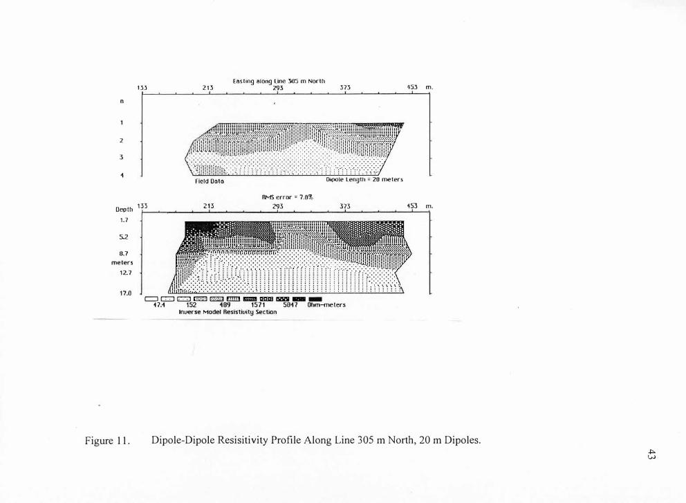
In order to evaluate the possible changes in reflection frequency along the line,

a spectral analysis was completed for 4 stacked traces located at 199 m East, 321 m

East, 352 m East, and 482 m East. The spectral analysis was computed over the entire

vertical length of the scan using RAD AN III and does not appear to have energy

normalization from scan to scan. The results of the spectral analysis of the stacked

traces are shown in Figure 15. Each spectral analysis shows similar results, with the

traces at 321 m East, 352 m East, and 428 m East showing more low frequency

content than that of the trace at 199 m East. For reference, the traces at 321 m East

and 352 m East are located within the plume region, and the traces at 199 m East and

428 m East are located outside of the plume region.

48

,

IIACNITUl)I

1.11

.. ,

II.II I-'.._,.-

IIACNITUDI 1.11

.. ,

Figure 15.

Legend:

35

33

50

y� -; bn

75 11111 CYCLES/ICIIN

,a 73 11111 CYCLES/ICIIN

GPR Sp�ctral Analysis Along Line 305 m North.

IIACNITUH 1..11

,.,

I � 8,8 r' V

IIACNITDH 1,1

1;,

35 50 75 lBB CYCLES/ICIIN

1,1f"Y !1 , ' � :p I

33 38 75 11111 CYCLES/I CAN

Clockwise from top left: 199 m East, 321 m East, 352 m East, 452 m East .i::,. '-0

.. A . - ~ 8 I

. --- ' CM -- -•

CHAPTER V

INTERPRETATIONS

Geophysical Results

Six different geophysical methods were used in an attempt to identify the

nature and location of a contaminant plume associated with hydrocarbon

contamination. Each method was first evaluated separately and then a final joint

interpretation was developed. All interpretations were based on the assumption that

there is a conductive plume associated with the dissolved hydrocarbon plume in the

ground water.

Self Potential

The self potential contour plot (Fig. 5) had a high positive anomaly running

through the center of the survey area. Based on the facts that non-polarizing

electrodes were used, and that there are no known mineral deposits underlying the

site, the SP anomaly is due to one of the hydrochemical potential mechanisms. A

likely source for this potential could be the presence of a conductive plume in ground

water. The conductive plume has a different concentration of ions and different

electrochemistry from that of the uncontaminated areas. When the two regions are

50

measured relative to one another, an anomaly can result due to the concentration

potential and the diffusion potential (Corwin, 1990). The maximum magnitude of the

potential is + 16 m V above background, which would indicate a change in ground

water conductance. This change in ground water conductance is based on the Nemst

potential, which is generated from two fluids at different concentrations, and can be

positive, unlike mineralization potentials. The cause of the secondary anomaly to the

east of the NW-SE trending anomaly is unknown. The dissolved plume boundaries

defined by the chemical surveys by the NCIBRD are located to the west of this

anomaly. A possible mechanism for this anomaly is the presence of a drain or utility

pipe. If the pipe is constructed of steel, it will oxidize in the ground and produce a SP

anomaly that is similar in magnitude to that seen in the contour plot.

Mise-a-la-masse

The mise-a-la-masse contour plot showed very little deviation from the

circular trend (Fig. 6). The presence of the circular trend indicates that the down hole

current source did not act as a point but perhaps as a long vertical cylinder, primarily

contacting the vadose zone. This concept is reinforced when viewed in light of the

fact that the electrode was clipped to the casing of the cable tool drilled well FT-4D.

Assuming that the conductive plume should give an elongate anomaly with the

MALM data, the field data do not support the hypothesis. A likely reason for the lack

of any major trend over the plume is the use of the well casing as the current source.

51

The casing has rusted a great deal over the exposed length, and may not be

transmitting current below the first threaded joint. If this is the case, then the MALM

survey has simply measured potential drop in the vadose zone, which should not give

any deviation from concentric equipotential lines as no conductive plume is known to

reside in that region. The assumption that the current source was at the dissolved

plume depth is probably incorrect.

Vertical Electrical Soundin2s

The three VES surveys conducted over the area had many of the same

characteristics. Each showed a change from resistive layers near the surface to

conductive layers at depths. The inverse model for each VES is shown in Table 5.

The first 2 layers in VES # 1 and the first 3 layers in VES # 2 and VES # 3 are

interpreted to represent the vadose zone. There is a noticeable change from the

surface layer apparent resistivity from VES # 1, which is located above the plume,

and the surface layer and vadose zone apparent resistivities from the other two VES;

which are located off the plume. The lower surface layer and vadose zone apparent

resistivities over the plume indicate that some of the conductive ground water is

present in the vadose zone, and the degradation of the hydrocarbon is not limited

solely to the saturated zone. There is a great deal of variability in the saturated zone

apparent resistivities, which are represented by layer 3 for VES # 1, and layer 4 for

VES # 2 and VES # 3. The lowest apparent resistivity is from VES # 1, which is

52

Table 5

Inverse Models for Each VES

Apparent Resistivity and Thickness of Layer

VES# 1 VES# 2 VES#3

Layer 1 98nm 0.24m 363 2 nm 0.14m 363 1 nm 0.1 m*

Layer 2 1113 nm 6 m* 33000 nm 0.89m 330 86 nm 1.14 m

Layer 3 1 20nm 15.36*m 5600 nm 7.27m 6970 nm 6.84m

Layer 4 3 2nm 800nm 10.0 m* 4200nm 3.67m

Layer 5 not used 27nm 42nm

RMS error 16.8 23 % 11.2 23 % 6.27%

* - denotes parameter was held constant during inversion

located on the surface above the plume. The apparent resistivity for the saturated

zone in VES # 2 and VES # 3 is more than 25 times that of the VES # 1. This

indicates that there is a much more conductive ground water below VES # 1 than in

the other two. The lowest layer in each model represents the clay layer, with an

apparent resistivity ranging from 27 nm to 42 nm. The depth to the clay layer is

quite variable, in the inversion of VES # 3 the depth to clay was found to be less than

1 2 meters, which is highly unlikely. This anomalously shallow depth to clay is most

likely due to a problem of equivalence, as the apparent resistivity of 4200 nm for the

saturated zone is far too high for saturated aquifer sands. In order to evaluate the

53

effects of suppression and equivalence several models were run on VES # 1 and VES

# 3. Two inverse models were run on VES # 1, the results are shown below in Table

2. The results of the two inverse models are shown in Figure 8, and show that for the

electrically equivalent layer 3, the curves have a very similar appearance. Therefore

the values for the depth and resistivity of a given layer can be modified to give very

similar results. A similar set of forward models was run for VES # 3, and are shown

below in Table 4. The results of the varying the saturated zone apparent resistivity in

the two forward models for VES # 3 are shown in Figure 9. There are considerable

changes in the apparent resistivity with depth, but the two extremes for the model.

This example shows that by varying the apparent resistivity in a given layer can

produce similar results.

There are several problems associated with the VES surveys undertaken at the

FT-02 site. The VES method works best in an area that has horizontal layers of

uniform resistivity and thickness, and that have an infinite lateral extent. This is not

the case at the FT-02 site because the dissolved plume itself is not infinite in extent.

Also, the first two layers at the site were highly resistive, which has a degrading effect

on the measured potentials. A second problem is the presence of utilities and cables

within the subsurface. These bodies can provide an alternate path for the current, and

distort the VES curve. A third problem associated with this site is the number and

spacing between the VES surveys. If a series of VES surveys had been collected

along a line separated by a fixed difference, it may have been possible to identify

54

changes from contaminated and uncontaminated areas. The three surveys at this site

had different orientations and were located very far from one another.

Dipole-Dipole Resistivity Profilin�

The DDR profiles each show a shallow, low resistivity anomaly in the central

region of each survey. These anomalies had modified model depths of 2 to 4 meters,

indicating a conductive source in the vadose zone if the modified model depths are

correct. Also, there is no abrupt change at 6 meters, which is the depth to water table.

Since the water table should have a strong electrical contrast with the vadose zone, it

should appear distinctly on the model. The lack of this abrupt change indicates that

the inverse model generated by RES2DINV may not be well suited for accurately

determining horizontal layer thickness and resistivities using the DDR method due to

the Principle of Equivalence. The appearance of a conductive region in the vadose

zone cannot be corroborated by geochemical means, as all geochemical samples for

the FT-02 site are taken from the saturated zone. Overall, the field data show a

conductive anomaly, but the inversion model cannot uniquely determine the vertical

location of the conductive anomaly.

In light of the results from the inverse models, a series of forward models

were developed using RES2DMOD, a forward modeling program using the same

computer routines as RES2DINV. The model was run with and without a plume, and

included the vadose zone, the saturated zone and the silty clay layer. The result of the

55

model without the plume is shown in Figure 16, and the results of the model with the

plume are shown in Figure 17. The model without the plume has a sharp decrease in

apparent resistivity with depth, which is interpreted to be the program's representation

of the sharp contrast in apparent resistivity at the vadose zone - saturated zone

interface and the saturated zone - silty clay interface. It is interesting to note that even

at a 10 m dipole spacing, the silty clay layer has an effect on the measured

pseudosection. This is a good indication that the depths generated by the inverse

model are highly suspect, and may not represent the true depth. It is important to note

that the dome-shaped change in apparent resistivity at depth centered around 240 m is

an artifact of the modeling program, and does not represent any geological condition.

The model with the plume showed the same decrease in resistivity with depth, but

superimposed upon the sharp vertical gradient is a three peaked low resistivity zone

located over the area where the plume was modeled. This is the exact same signature

seen in the 10 meter dipole data from Line 305 m North, and is strong evidence for a

conductive plume. The larger dipole spacings over the plume showed a lesser effect

on the apparent resistivity pseudosections. Finally, the forward models were run

using different arrays at the surface, but there was no appreciable change from array

to array.

To briefly summarize, the two sharp resistivity interfaces appear to dominate

the pseudosection, creating a single zone of continuous steep gradient. The plume

56

in 0.0 8121.0

1

2

3

4

UAFB :ll.69

lF'r-�2 site 2:46

235 280

32� 40@1\1.

398 Apparent �esistivity CDipole-�ipoie) in OHH.� Unit Electrode Sp�cifig = 1G.@ �.

28 280 1itllili!l 1000

- - -

7. 0.�0.0

3.0

6.0

9.�

:ll.2

40.0 80.0 120 169 2010 240

Figure 16. Dipole-Dipole Resistivity Forward Model Without Plume.

280 320 360 4@@

v-,

---..)

ll1l 0.�

:ll.

2

3

4

8@.gJ l

Y�FB Ff-ij2 site l!.6� 241� 32®

- - lfflia limllll 11.11a - .mm mm Mm !ffl!lll!t!l - lll!IE

252 314 376 500

4\QIIBI M.

�P��lf'!?nt Resastnvnty <»a�ol�-�npoRe) im, OH�-� �mnt Eilectlt"Ode Sp�cn�� = :ll.0.9 M.

Figure 17.

30 280 10@11,J

- - -

ll.llill00 28 :ll.Sllill -

z ®·� 0.0

"ll0 .Ii!) 80 .0 1291 1691 290

3.0

6.0

'9J .0

l!..2

249

Dipole-Dipole Resistivity Forward Model With Plume.

280 320 360 <1100

V,

00

-.t28 :l9Q 438 -~ 562 -

produces a minor change superimposed on the sharp gradient. Several different

arrays were modeled over the site, but it appears that none of the models can

overcome the effect of the sharp interfaces. The dipole-dipole results are useful in

detecting the horizontal extent of the plume, but cannot resolve the depth effectively.

Electroma�netic Induction

The EM data (Fig. 13) show spike anomalies on both the EM-31 and EM-34

lines. These spike anomalies are interpreted to be utility pipes or cables in the

subsurface based on the strong conductivity and in-phase anomalies seen in the data.

The slight high in conductivity in the EM-31 data along line 305 m North

is located directly above the plume and is probably the effect of the conductive

dissolved plume, which is approximately 6 meters deep, the effective range limit of

the EM-31 instrument. Line 305 m North is the only EM-31 profile that shows a rise

in conductivity over the dissolved plume, the rest of the profiles on other lines show

no change over the dissolved plume. Since the top of the dissolved plume is located

from 5.5 to 6 meters below the ground surface, it is very close to the effective range

limit of the EM-31 instrument.

The results of the EM-34 show similar results over the utilities identified from

the EM-31 instrument. The EM-34 instrument shows a terrain conductivity low over

the area associated with the dissolved plume, from 260 m East to 330 m East. This is

a region where a high terrain conductivity was expected, as the ground water

59

conductivities are higher in the center region of Line 305 m North than in the distal

regions. A possibility for the low terrain conductivity anomaly is a geometric

constraint on the method. The dissolved plume is only 60 meters wide at most points,

which is only 3 times the width of the coil spacing. It is possible that the EM-34 unit

will spatially alias the plume at this particular coil spacing and give an anomaly that

has a low centered around the dissolved plume.

In order to evaluate the effect of the plume at depth, a series of forward

models were developed for the EM-31 and EM-34 using PCLOOP, a forward model

designed to model EM data. Four models were run, two with a 0.5 m thick plume and

two without. The model data are shown in Table 6. Models 1 and 2 represent a plume

with a vadose zone apparent resistivity of 5000 nm and 1000 nm, respectively.

Models 3 and 4 represent clean areas with a vadose zone apparent resistivity of 5000

nm and 1000 nm, respectively. The results of terrain conductivity are shown below

for the horizontal loop configuration in Table 7. The forward model input parameters

are based on apparent resistivity values from the dipole-dipole and VES surveys, and

the resulting terrain conductivity is 3 to 4 times lower than what was measured in the

The values are assumed to be scaled to one another, and can represent the percent

change when comparing non-plume to plume areas. Overall, the change from non­

plume to plume areas appears to have a significant effect on the measured terrain

conductivity. It appears to have the biggest change when measured with the EM-31,

and the lowest change when measured with the EM-34 at the 20 meter coil separation.

60

Table 6

Forward Models for Electromagnetic Induction

Apparent Resistivity and Thickness of Layer

Model 1 Model2 Model3

Layer 1 5000 Om 1000 Om 5000 Om

5.5 m thick 5.5 m thick 5.5 m thick

Layer 2 80Om 80Om 150Om

0.5 m thick 0.5 m thick very thick

Layer 3 150Om 150Om NIA

very thick very thick

Table 7

Results of Electromagnetic Induction Forward Models

Model 1

EM -31 1.83

EM-34 (10m) 3.68

EM -34 (20m) 4.98

Terrain Conductivity in mS/m

Model 2

2.36

3.86

5.09

Model3

1.71

3.51

4.87

Model 4

1000 Om

5.5 m thick

150Om

very thick

NIA

Model 4

2.25

3.79

4.99

61

This response is expected, as the EM-34 samples a much greater volume than the

EM-31, and the conductivity changes do not change as much as the volume. It cannot

be determined whether it is possible to detect the degrading plume, as the changes are

only 2 - 7% of the measured terrain conductivity.

Ground Penetratin� Radar

The two representative GPR profiles show very similar results. An area of

attenuation, or shadow zone, is coincident with the plume along all lines. The

attenuation is a direct result of the low electrical resistivity of the dissolved plume as

it is almost entirely below the water table. The transition to attenuated signal is very

sharp, and occurs regularly at or below the 80 nanosecond level on the time records.

A measurement of the average dielectric permittivity for the vadose zone by using the

radar travel time and the known depth to water table at a nearby well gives Er= 8.3

and resulting velocity of 0.104 m/ns, which correlates well with the vadose zone

velocities given by Daniels (1989).

Performance of the Methods

The mise-a-la-masse method had no success in detecting the conductive

anomaly because of errors in the setup of the MALM survey. A proper setup would

involve the direct placement of an electrode into the conductive plume by means of a

62

push tool. Also, a resistivity meter with a higher input current should be used in order

to survey further from the downhole electrode

The vertical electrical sounding method had a limited success in detecting the

anomaly. The method could detect an anomalous region, but could not assign a

proper depth to the anomaly which, due to the Principle of Equivalence, can only be

overcome by "calibrating" against coincident borehole conductivity logs or measured

depths to interfaces in a borehole. As mentioned earlier, a linear array of soundings

could provide a better picture of the contamination. Also, by deploying a row of

soundings with a fixed interval between them, a meaningful joint interpretation could

be calculated for the layers derived in the individual inversion models.

The dipole-dipole resistivity method had some success in detecting the

anomaly. The inverse models suffered from the same lack of absolute depth control

due to the Principle of Equivalence, but the raw data pseudosections themselves

showed the general region of contamination. The inverse models did locate the

horizontal boundaries of the conductive plume to the level of resolution possible in

dipole-dipole resistivity surveys. The use of forward models to depict the plume

boundaries showed that the sharp contrast in resistivity at the vadose zone - saturated

zone interface and the saturated zone - silty clay layer combined to produce a single

steep gradient zone which dominated a large portion of the pseudosection

measurements, and almost masked the conductive plume.

63

The electromagnetic induction method as applied did not have any success in

detecting the conductive plume. The method was well suited for locating utilities and

cables, but did not show a large increase in ground conductivity over the plume itself.

It is believed that the plume is located too deep to be resolved by the EM-31 unit, and

is not conductive nor thick enough to be resolved with the 20 meter coil spacing on

the EM-34 unit. There is a 10 meter coil spacing for the EM-34, so a survey run with

that particular coil spacing may show the anomalous conductive region.

The self potential and ground penetrating radar methods both were very

successful in detecting areas of known contamination. The SP plot had some features

extending beyond the known dissolved plume in the eastern edge of the site, perhaps

due to an interfering source, but the GPR method worked well at resolving the

vertical and lateral plume boundaries. The GPR method is highly sensitive to the

input parameters of record length and gain function. If the record length had been set

to 100 nanoseconds, the amplitude anomaly probably could not have been detected.

The GPR survey acquisition parameters must be inspected closely, and several

parameters should be adjusted to gauge the effect of the parameters on the detection.

The combination of results from the VES surveys into the forward models for

the dipole-dipole and EM surveys allowed for meaningful comparisons of the various

methods. Also, by measuring the expected response of a survey over a plume, the

surveys could then be evaluated based on the expected response. By integrating the

results from the GPR, SP, Dipole-Dipole, and VES surveys, a clear and consistent

64

picture of the plume was developed, and the specific shortcomings of each survey

could be overcome.

Conclusions and Recommendations

The conductivity of a hydrocarbon plume is highly dependent on which region

of the plume is being measured and the age of the plume. At the FT-02 site, a

conductive anomaly was found to be coincident with the dissolved plume. It may be

possible that a hydrocarbon plume undergoes a change from resistive to conductive

behavior over time, but that temporal progression was not evaluated at the FT-02 site.

Further geophysical studies on the evolution of a hydrocarbon plume from the start of

contamination could shed light on how a LNAPL plume changes over time.

There are several ways to improve the performance of the methods discussed

in this project. The YES method could be applied in a regular and repeated fashion to

investigate if changes over a site can be traced from the source of a plume to regions

down gradient. The dipole-dipole resistivity method could use shorter (5 meter)

dipoles in order to evaluate the depth resolution of the method at this site. New tools

and methods such as bore hole EM tools and the vertical resistivity probe can give

information about the vertical extent of the plume, which has not been unambiguously

established by the geophysical studies at FT-02.

Finally, a more in-depth analysis of the chemical data could yield information

about the specific zones of chemical alteration and biodegradation of the residual and

65

dissolved plume. It may be possible to detect and delimit the various zones, and the

amount and rate of plume degradation taking place. Very little chemical information

was made available for this project, but a more intensive study may lead to a better

understanding of the degradation and what methods are best suited to measure it.

The interpretation of the field studies has shown that a degrading hydrocarbon

plume shows a decrease in the electrical resistivity. This electrical resistivity low is

located in the top portion of the saturated zone, and is less than half the electrical

resistivity in the uncontaminated areas. This study clearly shows that a hydrocarbon

plume in the field can exhibit electrical resistivity that is the complete opposite of

theoretical models.

66

Appendix A

Organic Chemicals Detected in July 1996

67

68

r1L

-� con�ed: 071091V6 • 07/11196 National Cen:;:

;::,.ra.: :=:..

mecr�lion

���

by Encotec: 07/23196 • 07/25196

•-• In• I ..,..... �

Bonzene -----------f-- Nl _ . _ Nl · _ 45 -'. 8� • Nl--J_ tn;:2 . __ Nl _ _j_ . Nl ___ t,!) ___ IIO

�':'��nzene ·--j-- �---- '.- � - '. · � ·i- � . -�--: ···· � · · -� J-· � -�- -�--+----1

:.roo::=::: ------L .. �-----�---�---�-J ... � '---� L=:: -�--L -� _ � � : �- I Nl N) t.n:t.n t.n: Nl WI Nl N) ��

�:'.'i'�1-�.:=� -�:� � : �� �-,--:-,�o __ l: 1�0 .:..� =L...1�o.e �-.:.J��-�-- :=:..�- ---�--- ----� .. - -+ N) . 43 : 110 • 170 ' t.n ' t.n N) •• N) to Tetrachlor�lhene. ·----·-- 1:D. __ Nl ... IP. .to .. a •. t'l ·l _!,[)_ •. l'.O. ..to_ _!{)___ .N:!. -_t __ -__ -_ -.. ·. Toluene . . . ______ ____ Nl__ -�- .1. 1_ . --�'- .N:!.. _,-o__ _ N)_ . . .I\O .. . _Nl__ •. !'O .

. 1...L ••Tricllloroethan• to Nl Nl N) N) Nl N) Nl N) N) I TrichlofO!!lbeDL --·-·····- __ _N)_ .. . _N)_ .l:Q . .to. ..lit. ..NL.. Kl. . _Nl_ .

. -�- .... --�-.. .

j ·-· __ _ ,�";!���--- ---·-· -�-- ... * -�"- ! -�- � ! �--- �-- - --�-. N) N) +-

m-Xytone&p-J(yllne ____ _ _ _ .. _l'Q ___ .• 1.I .0 ·-;- ··-�O. r�S.0-:

···10- ·-i--� _ I\O __ ±· __ 9_. ___ tp _ _ -� Nl=-�---------·--·-- - -• •--•• • --•-•- •• ;" •- --• i -

I • •---t---- • ••-- 1 -- • -

•- -•----+--•- -

cls·1,2-0ld)l_.l!!t!!t__ ____ , � • · •..• NJ. '.to · ___ ,ti;! ___ :_. __ jf,Q4•"_-_i ·---�------ _"lL__ ..

. ...N> _____

N)� ..

.. ===--.......!.--== Ell)ylbenz-..._______ __l.Q ___ IQ ...• : .. _Nl_ • "-"· ..., 2 __ .. __ Nl . Nl _ _j_ __

It!!• .. N) : N) N) N) • N) N'> N'> N) N) Io!u•ne _____________ +·- _t-p ____ t,g__�---ffi-. , __ ID _ _'.. _JQ ___ L._..W_ . _tp __ --�---�I\O�-+----t-----

i���;.ll!l� � ➔-�-: -�- - -�-+- �--+-•-�- ---: � --�--------·

V!l)YI �--- N) : re , Nl_ ··+--t3 __ i __ 11__...L._N)__ _ JP. Nl -�N)""'----,r----+----·I !t�yle,:,L_ N) ! tQ__j___l\O __ �IQ i 6 I N) �Nl,c. --+--�N)�-t-�N)C---t----t----l �x� "°-r-"° ' toia,1.anl N) N) N) "°

I ! I 1--------------t--�-+----,----t---+----+----+-----t-----,r----t----+-----l :

I -,.:---+-,---t-:---t----t-----J·----+----+----l

-� Nl I N) Nl t.n I 7 ' <7 A 4• Nl Nl Nl Nl i Chi--�----- t.n I N'> t.n 1 • I t.n t.n t.n N) N) N) N) 1 4.~...__,_!lll!l" Nl I Nl , r,o r,o I r,o r,o r,o r,o Nl Nl to .11:�.ne�

------+

-�Nl-

--+-,�IQ_j__J.Q .J____Hl I N> r,o N> Ni NJ t.n t.n

1 N) N) 1 Nl i Nl I Nl N) N) Nl Nl t.n t.n

' ,.� ·- �--.,. I -i- -- - .

� FT1.Cn I JC: rliliil. I "11:C::: .

. : n,m I �4- F ::-rl■C" c---.. DI---- "P'..l.- 1"11--1.

.l!!!:\Ur!e �

__ Nl __ , __ NL.-+--tQ. ____ . _t()__J _ _N> Nl •. .JP _ __tp_. to '° �!M � N) I N) I � . _! N)---i,c N) N) Nl • Nl ID 1•- N) r--,o . N) ' Nl I N) N) N) Kl N) '°

J.� Nl I !O W --� "° N> ...H2___-1P. to '° 1,2· � I re. N) · N) • l'D__i Nl N) N) � ID

li.1-. Nl Nl Ml . io� Nl I ;:,;-- r,o- to '-c"' Nl--

t-�c"-

-+- -

---1

l!rl�.thene Nl N) I IO_ +-� I Nl y!')1� N) to......J_t,O_ N I 1-Q

N) N'l

·o.n N) N)

N) N'l t.n N) Nl

1<>-X......_ N) N) I N'l i Nl I N'l N) N) N'l

'.NO • No Detection Concentration • ug/L

t.n t.n

1996 Quarterly Sample Rts1Atsl2 Report Printed: 1017/96

.. F "01

-· -. . - ...-~--

I I

r

I I

Vdf'ilc PtATCf-•-,----,--,----t - - Erm - : ffis : . ma-·-~ -ms -; ifiw+ EIZl - - EJ1as -~-- EilQQ EIJris- ·- ---t-----< l•~""'~.,~"'L-"_"'._~°'._~~-:_-_-:_-_-_-:_-:_-_,.w~-•~•~JO~-•:;:_-~..J:.,,':_""_-:_-_-_-:_-:_~.,,"'..':_':_-:_-:_-:_-:_~'",.Nlt":_-:_-:_,-:_-:_"':1:,~:::~_•4:1:0_•:~1:_-~:Nl:~:~;:~_,tNl'"',_':_-:_-:1':_-:_~"':.,,:_•:1:~~:.,,:~:j,..-:::_-_-_-;_· ___ -J

_fr;:=~'----------- ; ---~--~ ---t · _; L .~. ~-i i !-- i · --~ - -~ -- -- ·-· 1.

--1 - I

' -! I I

- - l I I

- - --- -1--- - - • I I I I I I I I

I I I I I

1------------ ----:--- - -------- I ~-,n- I ~~1n 1 I ~,,~

I I 1 I I -I I I -- -~ --- I

I N)

N) N) N'l N'l

_El/>~-- =t-~--:- _M)--i- --~- . ;- N)1 I N)N)-~ ~ - _ .lPN).. F _N)N) __ __!,QN)···-1,1,ach!q,:qethene _ •~ t-_Hl_J._ _ ru . .. ·1--"·- ·l ---~ -- _ ___ _ __ -- ~:c--+-~""---Tol····· N) o.n ' N) ! N) I N) , o.n M N) N)

N) N'l

N? N) N'l N'l N) N) N) N) .,, .,, N) N) N) N)

•~ -.-n:C-•---~- .. ---- ---- ----~'~--,

:- ---+-----+-- - ---l --,·-

_j__ lw,a•.1~!L-~.!!.!!!!-".!L."----J·- - tp__L_lQ-+-to- ~'-~N)"--+--NJ-=i- .,, i;il·.l.2·,.,....•-·"'-· N) I .,, I !':P. I N> !'e II .,,!':P.

N) I N)-r-t.n - i .,, N,

1,1rag)!Q!l>!=lhe= ne~-------+- ~N)0 ~ _ _,_1 -~N)- 1 IIP_. I N) I N)

--- --1:0 .,, .,,

-t-- - t.n

t.n .,., N)

Tofuolle N) I to : N> . . I N) l.1t...!,1 Ja1•:.,T-.1112~rhl!!il!!ll"~:r-•'t!!Jh~·-!!L·- -----t-"'- .!:!.!N)~__;,-..!:!N>,L_ , N _J ~ Nl=---+,-~N')L"--+--- --t--- --+-~ ~ -1-- -

1 _..ll, ..... _ __J"'-..... ---""'--+---+---- ---l-..a'-+-N) N'l .,, -------- --+---- -i-1 - t.n

I N) I Nl Nl N) t.D

t.n N) t.n N) N) N) to N) N) N)

N'l .,, .,, .,, .,., N) N) N) M) on

Appendix B

Coincident EM-31 and EM-34 Profiles

69

-40

E

�

EM-34

._.

� ·5

ts 0 :::J

'U C

8 C

-��

-40

-40

E

� EM-31

._.

� ">

ts 0 :::J

'U C

8 C

-��

-40

200 400

Easting (m)

Figure 18. Coincident EM-31 and EM-34 Profiles Along Line 290 m North

70

-40

E EM-34

� ._

� ·5

ts 0 :::J

"'C C

8 C

-��

-40

-40

E

�

EM-31

._

� ·5

ts 0 :::J

"'C C

8 C

-��

-40

200 400

Easting (m)

Figure 19. Coincident EM-31 and EM-34 Profiles Along Line 274 m North

71

-40

E

� EM-34 ._. � ">

t) 0 :::J

"'C C

8 C

-��

-40

-40

E

� EM-31 ._. � ·5

t) 0 :::J

"'C C

8 C

-��

-40

200 400

Easting (m)

Figure 20. Coincident EM-31 and EM-34 Profiles Along Line 259 m North

72

Appendix C

Permission to Use NCIBRD Files

73

ICIBRD ilifflffili � ••••···········

••••···········

•••............

•............. . . . ........

National Center for Integrated Bioremediation Research and Develop university of michigan • department of civil and environmental engineering • wurtsmith air force base • 4140 e. california street • oscoda, michigan 487'14

1 0/ 3 1/ 9 6telephone: 517-739-0185 • lax: 517-739-0186

Mike Nash

Dept. of GeologyCollege of Arts and SciencesWestern Michigan UniversityKalamazoo, MI 4 9 008

Dear Mr. Nash,

My staff and I have compiled most of the information that yourequested in your 9/4/96 letter. I have included: • well logs• water chemistry data• USGS geologic information• well information (NAD19 2 7, NAD19 83)• water levels • FTA-02/OT-16 grid node locations• volatile chemical information form NCIBRD and AF records

Some of this information is provided on disk and the rest 1s mhard copy. I have not yet compiled the sieve data that you requested, but I will send it to you at a later date. I you have anyquestions about this information, please call me at (517) 739 0185.

We would appreciate a copy of the final report that you produce from this information. Please include SERDP and NCIBRD inthe acknowledgments of any deliverables that utilize the informationthat we have provided to you.

cc. M Barcelona, NCIBRDP Laird, NCIBRD files

Sincerely, �/.-/�rk �ry

,·

BIBLIOGRAPHY

Applegate, J.K., and Rodriguez, B.D., 1988, Integrated geophysical mapping of

hazardous plumes in glacial terrain, in Symposium on the Application of

Geophysics to Engineering and Environmental Problems, 1st, Golden, Colo.,

1988, Proceedings: Golden, Colo., Engineering and Environmental Geophysics

Society, p. 722-734.

Archie, G. E., 1942, The electrical resistivity log as an aid to determining some

reservoir properties: Trans. AIME, 146, p. 54-62.

Baedecker, M.J., Cozzarelli, I.M., Eganhouse, R.P., Siegel, D.I., and Bennett, P.C.,

1993, Crude oil in a shallow sand and gravel aquifer - III. Bigeochemical

reactions and mass balance modeling in anoxic groundwater: Applied

Geochemistry, v.8, p. 569-586.

Baedecker, M.J., Cozzarelli, I.M., and Hopple, J.A., 1987, The composition and fate

of hydrocarbons in a shallow glacial-outwash aquifer: U.S. Geological Survey

Open-File Report, p. 87-109.

Barcelona, M., May 1996, Personal communication.

Barker, J.F., Patrick, G.C., and Major, D., 1987, Natural attenuation of aromatic

hydrocarbons in a shallow sand aquifer: Ground Water Monitoring and

Remediation, v. 7, no. 1, p. 64-71.

Bennett, P.C., Melcer, M.E., Siegel, D.I., and Hassett, J.P., 1988, The dissolution of

quartz in dilute aqueous solutions of organic acids at 25° C: Geochimica et

Cosmochimica Acta, v. 52, p. 1521-1530.

Bennett, P.C., Siegel, D.I., Baedecker, M.J., and Hult, M.F., 1993, Crude oil in a

shallow sand and gravel aquifer - I. Hydrogeology and inorganic geochemistry:

Applied Geochemistry, v. 8, p. 529 - 549.

Brewster, M.L., Redman, J.D., and Annan, AP., 1992, Monitoring a controlled

injection of percloroethylene in a sand aquifer with Ground Penetrating Radar

and Time Domain Reflectometry, in Symposium on the Application of

Geophysics to Engineering and Environmental Problems, 5th, Oak Brook, Ill.,

75

.,_

•

..

. .... . ...

1992, Proceedings: Oak Brook, Ill., Engineering and Environmental

Geophysical Society, p. 611-618.

Campbell, D.L., Lucius, J.E., Ellefsen, K.J., and Deszcz-Pan, M., 1996, Monitorig of

a controlled LNAPL spill using Ground Penetrating Radar, in Symposium on

the Application of Geophysics to Engineering and Environmental Problems,

9th, Keystone, CO., 1996, Proceedings: Keystone, Colo., Engineering and

Environmental Geophysical Society, p. 511-517.

Corwin, R.F., 1990, Applications of the self potential method to engineering and

environmental studies, in Symposium on the Application of Geophysics to

Engineering and Environmental Problems, 3rd, Golden, CO., 1990,

Proceedings: Keystone Colo., Engineering and Environmental Geophysical

Society, p. 107-122.

Cozzarelli, J.M., Baedecker, M.J., Eganhouse, R.P., and Goerlitz, D.F., 1994, The

geochemical evolution of low-molecular weight organic acids derived from the

degradation of petroleum contaminants in groundwater: Geochimica et

Cosmochimica Acta, v. 58, no. 2, p. 867-877.

Cozzarelli, J.M., Eganhouse, R.P., and Baedecker, M.J., 1990, Transformation of

monoaromatic hydrocarbons to organic acids in anoxic groundwater

environment: Environmental Geology Water Science, v. 16, p. 135-141.

Daniels, J.J., Roberts, R., and Vendl, M., 1992, Site studies of Ground Penetrating

Radar for monitoring petroleum product contaminants, in Symposium on the

Application of Geophysics to Engineering and Environmental Problems, 5th,

Oak Brook, Ill., 1992, Proceedings: Oak Brook, Ill., Engineering and

Environmental Geophysical Society, p. 597-609.

DeRyck, S.M., Redman, J.D., and Annan, A.P., 1993, Geophysical monitoring of a

controlled kerosene spill, in Symposium on the Application of Geophysics to

Engineering and Environmental Problems, 6th, San Diego, Ca., 1993,

Proceedings: San Diego, Ca., Engineering and Environmental Geophysical

Society, p. 5-20.

Dobrin, M.B., and Savit, C.H., 1988, Introduction to Geophysical Prospecting ( 4th

ed.): New York, N.Y., McGraw-Hill, 867 p.

Eganhouse, R.P., Baedecker, M.J., Cozzarelli, J.M., Aiken, G.R., Thom, K.A., and

Dorsey, T.F., 1993, Crude oil in a shallow sand and gravel aquifer - II. Organic

geochemistry: Applied Geochemistry, v. 8, p. 551-567.

76

.

Endres, A.L., and Greenhouse, J.P., 1996, Detection and monitoring of chlorinated solvent contamination by thermal neutron logging: Ground Water, v. 34, p. 283-292.

Endres, A.L., and Redman, J.D., 1993, Modeling the electrical properties of porous rocks and soils containing immiscible contaminants, in Symposium on the Application of Geophysics to Engineering and Environmental Problems, 6th, San Diego Ca., 1993, Proceedings: San Diego, Ca:, Engineering and Environmental Geophysical Society, p. 21-38.

Fetter, C. W., 1994, Applied Hydrogeology (3d ed.): New York, N.Y., Macmillan, 691 p.

Gajdos, V. and Kral, V., 1995, Influence of hydrocarbon pollution to soil conductivity, in Symposium on the Application of Geophysics to Engineering and Environmental Problems, 8th, Orlando, Fl., 1995, Proceedings: Orlando Fl., Engineering and Environmental Geophysical Society, p. 785-789.

Grumman, D.L., and Daniels, J.J., 1995, Experiments on the detection of organic contaminants in the vadose zone: Journal of Environmental and Engineering Geophysics, v. 0, p. 31-38.

Loke, M.H., and Barker, R.D., 1996, Rapid least-squares inversion of apparent resistivity pseudo section by a quasi-Newton method: Geophysical Prospecting, V. 44, p. 131-152.

Maxwell, M., and Schmok, J., 1995, Detection and mapping of an LNAPL plume using GPR: A case study, in Symposium on the Application of Geophysics to Engineering and Environmental Problems, 8th, Orlando Fl., 1995, Proceedings: Orlando, Fl., Engineering and Environmental Geophysical Society, p. 15-23.

Mazac, 0., Benes, L., Landa, I., and Maskova, A., 1990, Determination of the extent of oil contamination in groundwater by geoelectrical methods, in Ward S.H.,ed., Geotechnical and Environmental Geophysics Vol. II, Tulsa, Ok, Society of Exploration Geophysicists. p.107-112

McMahon, P.B., and Chapelle, F.H., 1991, Microbial production of organic acids in aquitard sediments and its role in aquifer geochemistry: Nature, v. 349, p. 233-235.

McNeil, J., 1994, Problems associated with using ground penetrating radar to locate a LNAPL plume: Kalamazoo Mich., Western Michigan University, M.S. thesis, 55 p.

77

..

McNeill, J.D., 1980, Electrical terrain conductivity measurement at low induction numbers, Technical Note 6: Mississauga, Ontario, Canada, Geonics Ltd., 15 p.

Merrick N .P ., 1977, A computer program for the inversion of Schlumberger sounding

curves in the apparent resistivity domain: Hydrogeological Report# 197715, Water Resources Commission, N.S.W. Australia, 36 p.

Monier-Williams, M., 1995, Properties oflight non-aqueous phase liquids and

detection using commonly applied shallow sensing geophysical techniques, inSymposium on the Application of Geophysics toEngineering and Environmental

Problems, 8th, Orlando, Fl., Proceedings: Orlando, Fl., 1995, Engineering and Environmental Geophysical Society, p. 1-13.

National Center for Integrated Bioremediation Research and Development, 1996, Open Files. Unpublished Computer Files.

Redman, J.D., DeRuck, S.M., and Annan, A.P., 1994, Detection ofLNAPL pools with GPR; Theoretical modeling and surveys of a controlled spill, inInternational Conference on Ground Penetrating Radar, 5th, 1994, Kitchener, Ontario, Canada, Proceedings: Kitchener, Ontario, Canada, p.1283-1294.

Robins, G.A., McAninch, B.E., Gavas, F.M., and Ellis, P.M., 1995, An evaluation of

soil-gas surveying for H2S for locating subsurface hydrocarbon contamination:

Ground Water Monitoring and Remediation, v. 15, no. 1, p. 124-132.

Sauck W.A., 1990, Modification of the SCHLINV program - Internal Report, Institute for Water Sciences, Western Michigan University, Kalamazoo, Mich.

Schneider, G.W., and Greenhouse, J.P., 1992, Geophysical detection of perchloroethylene in a sandy aquifer using resistivty and nuclear logging

techniques, in Symposium on the Application of Geophysics to Engineering and Environmental Problems, 5th, Oak Brook, Ill., 1992, Proceedings: Oak Brook,

Ill., Engineering and Environmental Geophysical Society, p. 619-628.

Telford, W.M., Geldart, L.P., and Sheriff, R.E., 1990, Applied Geophysics (2d ed.): Cambridge, U.K., Cambridge University Press, 770 p.

78