Geomorphic change detection using historic maps and DEM ...
18
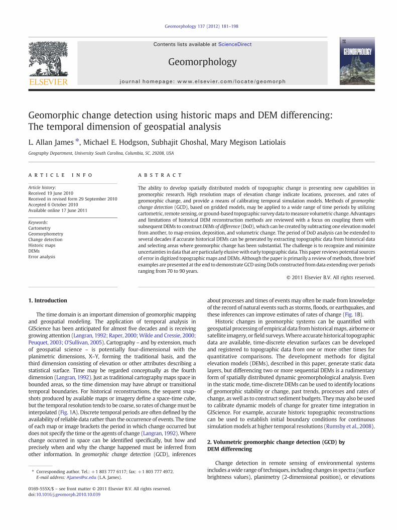
Geomorphic change detection using historic maps and DEM differencing: The temporal dimension of geospatial analysis L. Allan James ⁎, Michael E. Hodgson, Subhajit Ghoshal, Mary Megison Latiolais Geography Department, University South Carolina, Columbia, SC, 29208, USA abstract article info Article history: Received 19 June 2010 Received in revised form 29 September 2010 Accepted 6 October 2010 Available online 17 June 2011 Keywords: Cartometry Geomorphometry Change detection Historic maps DEMs Error analysis The ability to develop spatially distributed models of topographic change is presenting new capabilities in geomorphic research. High resolution maps of elevation change indicate locations, processes, and rates of geomorphic change, and provide a means of calibrating temporal simulation models. Methods of geomorphic change detection (GCD), based on gridded models, may be applied to a wide range of time periods by utilizing cartometric, remote sensing, or ground-based topographic survey data to measure volumetric change. Advantages and limitations of historical DEM reconstruction methods are reviewed with a focus on coupling them with subsequent DEMs to construct DEMs of difference (DoD), which can be created by subtracting one elevation model from another, to map erosion, deposition, and volumetric change. The period of DoD analysis can be extended to several decades if accurate historical DEMs can be generated by extracting topographic data from historical data and selecting areas where geomorphic change has been substantial. The challenge is to recognize and minimize uncertainties in data that are particularly elusive with early topographic data. This paper reviews potential sources of error in digitized topographic maps and DEMs. Although the paper is primarily a review of methods, three brief examples are presented at the end to demonstrate GCD using DoDs constructed from data extending over periods ranging from 70 to 90 years. © 2011 Elsevier B.V. All rights reserved. 1. Introduction The time domain is an important dimension of geomorphic mapping and geospatial modeling. The application of temporal analysis in GIScience has been anticipated for almost five decades and is receiving growing attention (Langran, 1992; Raper, 2000; Wikle and Cressie, 2000; Peuquet, 2003; O'Sullivan, 2005). Cartography – and by extension, much of geospatial science – is potentially four-dimensional with the planimetric dimensions, X–Y, forming the traditional basis, and the third dimension consisting of elevation or other attributes describing a statistical surface. Time may be regarded conceptually as the fourth dimension (Langran, 1992). Just as traditional cartography maps space in bounded areas, so the time dimension may have abrupt or transitional temporal boundaries. For historical reconstructions, the sequent snap- shots produced by available maps or imagery define a space-time cube, but the temporal resolution tends to be coarse, so rates of change must be interpolated (Fig. 1A). Discrete temporal periods are often defined by the availability of reliable data rather than the occurrence of events. The time of each map or image brackets the period in which change occurred but does not specify the time or the agents of change (Langran, 1992). Where change occurred in space can be identified specifically, but how and precisely when and why the change happened must be inferred from other information. In geomorphic change detection (GCD), inferences about processes and times of events may often be made from knowledge of the record of natural events such as storms, floods, or earthquakes, and these inferences can improve estimates of rates of change (Fig. 1B). Historic changes in geomorphic systems can be quantified with geospatial processing of empirical data from historical maps, airborne or satellite imagery, or field surveys. Where accurate historical topographic data are available, time-discrete elevation surfaces can be developed and registered to topographic data from one or more other times for quantitative comparisons. The development methods for digital elevation models (DEMs), described in this paper, generate static data layers, but differencing two or more sequential DEMs is a rudimentary form of spatially distributed dynamic geomorphological analysis. Even in the static mode, time-discrete DEMs can be used to identify locations of geomorphic stability or change, past trends, processes and rates of change, as well as to construct sediment budgets. They may also be used to calibrate dynamic models of change for greater time integration in GIScience. For example, accurate historic topographic reconstructions can be used to establish initial boundary conditions for continuous simulation models at higher temporal resolutions (Rumsby et al., 2008). 2. Volumetric geomorphic change detection (GCD) by DEM differencing Change detection in remote sensing of environmental systems includes a wide range of techniques, including changes in spectra (surface brightness values), planimetry (2-dimensional position), or elevations Geomorphology 137 (2012) 181–198 ⁎ Corresponding author. Tel.: + 1 803 777 6117; fax: + 1 803 777 4972. E-mail address: [email protected] (L.A. James). 0169-555X/$ – see front matter © 2011 Elsevier B.V. All rights reserved. doi:10.1016/j.geomorph.2010.10.039 Contents lists available at ScienceDirect Geomorphology journal homepage: www.elsevier.com/locate/geomorph
Transcript of Geomorphic change detection using historic maps and DEM ...
Geomorphology 137 (2012) 181–198
Contents lists available at ScienceDirect
Geomorphology
j ourna l homepage: www.e lsev ie r.com/ locate /geomorph
Geomorphic change detection using historic maps and DEM differencing:The temporal dimension of geospatial analysis
L. Allan James ⁎, Michael E. Hodgson, Subhajit Ghoshal, Mary Megison LatiolaisGeography Department, University South Carolina, Columbia, SC, 29208, USA
⁎ Corresponding author. Tel.: +1 803 777 6117; fax:E-mail address: [email protected] (L.A. James).
0169-555X/$ – see front matter © 2011 Elsevier B.V. Adoi:10.1016/j.geomorph.2010.10.039
a b s t r a c t
a r t i c l e i n f oArticle history:Received 19 June 2010Received in revised form 29 September 2010Accepted 6 October 2010Available online 17 June 2011
Keywords:CartometryGeomorphometryChange detectionHistoric mapsDEMsError analysis
The ability to develop spatially distributed models of topographic change is presenting new capabilities ingeomorphic research. High resolution maps of elevation change indicate locations, processes, and rates ofgeomorphic change, and provide a means of calibrating temporal simulation models. Methods of geomorphicchange detection (GCD), based on gridded models, may be applied to a wide range of time periods by utilizingcartometric, remote sensing, or ground-based topographic survey data tomeasure volumetric change. Advantagesand limitations of historical DEM reconstruction methods are reviewed with a focus on coupling them withsubsequent DEMs to constructDEMs of difference (DoD), which can be created by subtracting one elevationmodelfrom another, to map erosion, deposition, and volumetric change. The period of DoD analysis can be extended toseveral decades if accurate historical DEMs can be generated by extracting topographic data from historical dataand selecting areas where geomorphic change has been substantial. The challenge is to recognize and minimizeuncertainties indata that areparticularly elusivewith early topographic data. This paper reviews potential sourcesof error in digitized topographicmaps and DEMs. Although the paper is primarily a review ofmethods, three briefexamples are presented at the end to demonstrate GCD using DoDs constructed fromdata extending over periodsranging from 70 to 90 years.
+1 803 777 4972.
ll rights reserved.
© 2011 Elsevier B.V. All rights reserved.
1. Introduction
The time domain is an important dimension of geomorphic mappingand geospatial modeling. The application of temporal analysis inGIScience has been anticipated for almost five decades and is receivinggrowing attention (Langran, 1992; Raper, 2000;Wikle and Cressie, 2000;Peuquet, 2003; O'Sullivan, 2005). Cartography – and by extension, muchof geospatial science – is potentially four-dimensional with theplanimetric dimensions, X–Y, forming the traditional basis, and thethird dimension consisting of elevation or other attributes describing astatistical surface. Time may be regarded conceptually as the fourthdimension (Langran, 1992). Just as traditional cartographymaps space inbounded areas, so the time dimension may have abrupt or transitionaltemporal boundaries. For historical reconstructions, the sequent snap-shots produced by available maps or imagery define a space-time cube,but the temporal resolution tends to be coarse, so rates of changemust beinterpolated (Fig. 1A). Discrete temporal periods are often defined by theavailability of reliable data rather than the occurrence of events. The timeof each map or image brackets the period in which change occurred butdoes not specify the time or the agents of change (Langran, 1992).Wherechange occurred in space can be identified specifically, but how andprecisely when and why the change happened must be inferred fromother information. In geomorphic change detection (GCD), inferences
about processes and times of eventsmay often bemade from knowledgeof the record of natural events such as storms, floods, or earthquakes, andthese inferences can improve estimates of rates of change (Fig. 1B).
Historic changes in geomorphic systems can be quantified withgeospatial processing of empirical data fromhistoricalmaps, airborne orsatellite imagery, orfield surveys.Where accuratehistorical topographicdata are available, time-discrete elevation surfaces can be developedand registered to topographic data from one or more other times forquantitative comparisons. The development methods for digitalelevation models (DEMs), described in this paper, generate static datalayers, but differencing two or more sequential DEMs is a rudimentaryform of spatially distributed dynamic geomorphological analysis. Evenin the static mode, time-discrete DEMs can be used to identify locationsof geomorphic stability or change, past trends, processes and rates ofchange, aswell as to construct sediment budgets. Theymay also be usedto calibrate dynamic models of change for greater time integration inGIScience. For example, accurate historic topographic reconstructionscan be used to establish initial boundary conditions for continuoussimulationmodels at higher temporal resolutions (Rumsby et al., 2008).
2. Volumetric geomorphic change detection (GCD) byDEM differencing
Change detection in remote sensing of environmental systemsincludes awide range of techniques, including changes in spectra (surfacebrightness values), planimetry (2-dimensional position), or elevations

Fig. 1. Space-time cubes. (A) Geomorphic conditions at three discrete times (t1 throught3) with process rates assumed constant between each condition. With high temporalresolution reconstructions, conditionsat anypoint,Xi,Yi, Ti, in the cubecan theoretically beinferred. (B) Addition of known geomorphic events (e1, e2) and assumptions of stableconditions between events separated by step-functional changes during eventsmay allowrefinement of timing and identification of processes.(Adapted from Langran, 1992).
Table 1Methods of map comparison.(Adapted from Boots and Csillag, 2006).
1. Map accuracy assessments — comparisons with a reference map.2. Change detection — differences between maps or images collected at different
times.3. Model comparisons — comparisons of model output to observed landscapes or
to other model outputs.4. Landscape comparisons over time— similar to change detection, but focus is on
global (i.e., area wide) spatial metrics calculated from map data, and may beused to compare different geographical areas. Primarily used in landscapeecology but a growing trend in geomorphometry.
182 L.A. James et al. / Geomorphology 137 (2012) 181–198
(Jensen, 2007). Changedetectionmayprovidequantitativemeasures onacell-by-cell basis, but it can also reveal spatial patterns of change orchanges in pattern based on clusters of cells, which may be morediagnostic thanmagnitudes of change (White, 2006). Examples of recentstudies that have used DEMs for change detection in order to map ormonitor erosion, deposition, and volumetric changes, and constructsediment budgets include thework byMartínez-Casasnovas et al. (2004)andWheaton et al. (2009). Although digital terrain models (DTMs) maybe produced in a variety of data model forms, the following discussionassumes conventional two-dimensional arrays (cellular or finite-differ-ence) of orthogonally gridded elevation data. The term ‘DEM’ refers to thesquare-cell datamodel in this paper. The differencing of sequential DEMsto create a DEM of difference (DoD) or change in elevation grid isparticularly relevant to geomorphic studies because a DoDmay provide ahigh resolution, spatially distributed surface model of topographic andvolumetric change through time (Brasington et al., 2003; Rumsby et al.,2008). This formofGCD is apowerful tool thatmaybeused to identify andquantify spatial patterns of geomorphic change. Once two DEMs havebeen developed and registered to the same grid tesselation, a DoD can bemade by subtracting the earlier DEM from the later DEM:
ΔEij = Z2ij–Z1ij ð1Þ
whereΔEij is the i, j grid valueof the change in elevationmodel, Z1ij is thei, j value of the early DEM, and Z2ij is the i, j value of the later DEM. Theresulting DoD represents reductions in elevation as negative values andincreases in elevation as positive values. Determining the cause of thischange (e.g. erosion, deposition, subsidence, anthropogenic modifica-tion, precision, accuracy, or uncertainty) is more challenging.
Of particular interest to this study is the extraction of topographicdata from historical contour maps to allow construction of historical
DEMs for DoD analysis. Most DoD studies have been concerned withtemporal scales less than decadel based on field surveys or remotesensing data (Heritage et al., 2009). Historic reconstructions of greaterduration require historical imagery or the use of cartographic data.Cartographic data are especially important for reconstructions ofsurfaces prior to the availability of stereoscopic aerial photographs orin heavily vegetated areas where conventional remote sensingmethods cannot penetrate the canopy. If a high-resolution historictopographic map is available from a ground or canopy penetratingphotogrammetric survey, this map may be used to develop an earlyDEM for the area. Historical reconstructions based on analysis of aerialphotography can extend the time dimension back several decadesunder favorable conditions. The challenge of using historic remotelysensed imagery or topographic maps is first dependent on the sourcematerials and processing methods for their construction (Hodgsonand Alexander, 1990). For example, contour lines on many early (i.e.pre 1940s) topographic maps were “artistically” drawn with littleintervening field observations between field measurements. Modernmethods of topographic map construction (e.g. remote sensing based)use a comparatively dense set of observations (e.g. every few metersplanimetrically) for contour construction.
Themethods of volumetric change detection described in this paperare a subset of a broader set of comparisonmethods for spatial data. Fourtraditions in map or imagery comparison can be identified (Table 1).Comparisons may be made using cell-based or feature-based statisticsor with spatial patterns. This paper is primarily concernedwith the firsttwomethods— accuracy of historic spatial data andmethods of changedetection. It begins with the importance of extending historicalgeomorphic research and GCD back in time, followed by a briefsampling of past studies and examples of historical reconstructions andDoD analysis. Limitations and uncertainties associated with historicalreconstructions using maps, airborne imagery, DEMs, and DoDs aredescribed, emphasizing topographic maps that can be used to extendvolumetric GCD back in time. Finally, application of DoD analysis to anextended temporal scale is demonstrated with three case studies offluvial and hill-slope systems. DEMs are developed from early 20thcentury large-scale topographic maps and differenced with modernDEMs from aerial photographic stereo pairs or Light Detection andRanging (LiDAR) data to construct DoDs. These studies demonstrate theutility and limitations of the method for volumetric analyses of decadalto centennial change.
3. Importance of historical reconstructions
Historical reconstructions, GCD, andgeomorphometry are importantpotentials of geospatial analysis that will be of growing importance tostudies of global change and broad-scale anthropogenic impacts on theenvironment. The geomorphic effectiveness of anthropogenic changehas accelerated over historical time and interest in global change andclimate changehas grownaccordingly in recentdecades.Understandingthese processes requires a greater emphasis on historical knowledge ofgeomorphic systems. Time and space dimensions of geomorphicprocesses are closely linked. As the geographic extent of landforms

183L.A. James et al. / Geomorphology 137 (2012) 181–198
under consideration increases, the average rates of change decrease andthe relevant time span that needs to be considered increases (Fig. 2):
“As the size and age of a landform increases, fewer of its propertiescan be explained by present conditions and more must be inferredabout the past” (Schumm, 1991; p.52).
Given the strong scale dependency of process, accurate characteriza-tions of global geomorphic changes and calibrations of landscapeevolution models require a greater emphasis on historical studies.‘Historical’ in the context of this discussion of scale should be extendedto ‘stratigraphic’ or ‘geologic’ definitions of history, although this paper isprimarily limited to cartographic recordsnomore than150 years in age. Aperspective that links event-based processes to historical evolution isneeded for a better understanding of geomorphic responses that areglobally relevant. This article addresses GCD using geospatial technologywith historical maps and imagery to measure morphological change andidentify changes in processes over decadal and centennial time scales.Examples of these methods are reviewed and case studies are providedfor a variety of environments and geomorphic systems.
4. Previous studies of volumetric Geomorphic ChangeDetection (GCD)
Using historical spatial data to measure changes has a long history.Cartometryhas beenpracticedon relatively oldmaps topushGCDback intime (HookeandPerry, 1976). ThemainstayofGCDmethodsover the latetwentieth century has been planimetric analysis based on aerialphotogrammetric and field survey methods to generate DEMs at themeso scale (Lane, 2000; Lane et al., 2003; Hughes et al., 2006; Heritageet al., 2009). These methods have facilitated volumetric GCD not only forcomputing sediment budgets, but also to estimate sediment transportrates. For example, amorphometric method has been adopted by severalriver scientists as a means of computing bed-material transport rates ingravel-bed rivers. Measurement of bedload transport in gravel-bed riversis notoriously difficult (Gomez, 1991), so methods have been developedbased on sediment budgets from volumetric GCD. Topographic surveyscan be combined with digital terrain-modeling to quantify and monitorriver-channel changes (Lane et al., 1994). Increasingly, GCD is beingconductedwithmeasurements fromremote sensing asmethods improvefor measuring volumetric changes in shallow submerged bars (Gaeumanet al., 2003; Fonstad and Marcus, 2005; Marcus and Fonstad, 2008). Themorphologic method or inverse method uses volumes of sedimentcomputed from change detection to develop morphological sedimentbudgets to infer the rates of sediment transport in gravel-bed rivers(Ferguson and Ashworth, 1992; Lane et al., 1995; Ashmore and Church,1998; Brasington et al., 2003; Martin and Ham, 2005).
Fig. 2. Scale dependencies between magnitude and time for explaining geomorphicphenomena. Large geomorphic features and processes require a greater proportion ofhistorical understanding.(Adapted from Schumm, 1991).
5. Assessing data quality
Accurate GCD requires the reconstruction of one or more historicgeomorphic surfaces from which elevation changes can be computed.Thequality andconfidence in thehistorical topographicdata available areusually the limiting factors in the accuracy and confidence in the resultingGCD. Quantitative assessments of uncertainty range from the precision ofan instrument that was used to a full-blown uncertainty or error-budgetanalysis (Gottsegen et al., 1999;Hodgson andBresnahan, 2004;Wheatonet al., 2009). Uncertainties in source materials, processing methods,classification, resolution, completeness, image registration, interpolation,and other forms of error and error propagation should be recognizedbefore comparisons of sequential images are interpreted. A criticalevaluation of data sources, exercised early in the process, may lead to therejectionof potential cartographicorDEMdata sources formorphometricanalysis. In some cases, qualitative evaluations of features depicted
Fig. 3. Qualitative use of early maps may provide key information about geomorphicchange. (A) Excerpt of early map showing lower Yuba River, California (Von Schmidt,1859). Federal land survey corner sections (e.g. lower right corner) produced coordinatetransfer RMSE of 44 m (James et al., 2009). (B) Excerpt frommore accuratemap (Mendell,1881) shows position of 1879 channel and position of an undated earlier channel systemshownbydashed lines. Channel positionsderived from1859map are added to thismap assolid lines. (‘1879’, ‘1876’ and ‘1859’ labels added to original). These imagesweremanuallyedited to clarify linework and text from greatly enlarged originals, and to remove artifactsintroduced by map rectification.

Fig. 4. Accuracy and precision inmeasurements of a line from amap. Bold lines with soliddots represent reference layer, verticaldashed lines aremeanvaluesdefinedbyprobabilitydensity functions of measured observations. A) Precise and accurate. B) Precise butinaccurate. C) Accurate but imprecise. D) Inaccurate and imprecise.
184 L.A. James et al. / Geomorphology 137 (2012) 181–198
on maps may alter interpretations of apparent changes on maps. Forexample, rectification of an 1859 map that was not sufficiently accuratefor quantitative analysis of change was useful for qualitative referencingwith a more precise 1881map (Fig. 3). The north half of the 1859 sourcemapwas georeferenced to section corners of federal land survey resultingin a rectification accuracy of 44 m root mean square error (RMSE). Theactual uncertainties are presumably larger because of other errors notaccounted for, such as positions of survey corners on the map.Superimposition of the 1859 channel locations onto the more precise1881 map shows that the 1881 dashed lines correspond to the 1859channels, which allows dating of the 1881 features.
The feasibility of producing an accurate GCD increases as themagnitude of expected change increases; i.e., GCD quality depends onthe strength of the signal being measured relative to the data quality.This relationship may be expressed as a signal-to-noise ratio in whichthe signal is actual geomorphic change and noise is introduced byerror variability (adapted from Griffith et al., 1999):
S=N = VGC = VEP ð2Þ
where S/N is the signal-to-noise ratio, VGC is variability caused bygeomorphic change, and VEP is variability caused by errors. A high S/Nvalue is desirable. At low values approaching one, geomorphic change isno greater than the errors, and the degree to which changes are real orapparent becomes less certain. As written, Eq. (2) is difficult to apply,because total errors are difficult to compute and actual geomorphicchange is rarely known. Observed changes include errors and actualchange, so VGC must be estimated after errors are known. Nevertheless,the concept is useful as it expresses the feasibility of a successfulGCDas aninverse relationship between the degree of change and data quality. Ananalyst may be able to reduce data uncertainty, but geomorphicvariability is inherent to the system. Thus, systemswith large geomorphicchange are more conducive to GCD. Errors are difficult to determine, so aconservative estimate of S/N based on data uncertainty in thedenominator may be the appropriate measure. An important researcharea forDEManalyses going forwardwill be todevelop standardmethodsof computing S/Nvalues and, perhaps, establishing oneormore thresholdvalues for including analyses based on this criterion (cf. Wheaton et al.,2009).
Difficulties in distinguishing change from error can be seen in lateralshifts in apair of linesmeasured fromsequentialmapsor images. The linesmay represent the edge or crest of a landform, such as a stream bank ordune ridge. Evenwithnogeomorphic change, somedegree of line offset isto be expected as inherent error introduced by a variety of cartographic orphotogrammetric sources. Line offsets are commonly used as an errormetric (‘sliver’ analysis) in assessments of cartographic error (Chrisman,1989). The likely magnitude of such errors should be evaluated to assessthe confidence in the GCD. Some, but not all error may be removed orminimizedby image registration. Least squarepolynomial transformation,commonly used in map/image rectification, distribute the errors acrossthe study area and it is important to report these error statistics. Spatialerror statistics are often reported as aRMSE to estimate the potential errorcomponent in a GCD analysis. Alternatively, the Circular Map AccuracyStandard (CMAS) may be derived from the RMSE and reported for two-dimensional uncertainties (FGDC, 1998). These are not the only sources ofuncertainty, however, and other error contributions will increase theresulting error (and decrease confidence). Therefore, values of spatialaccuracy should be considered a minimum value of uncertainty in thedata.
Change detection should be performedusing historic data of sufficientquality to decrease the likelihood that much of the observed differencesare caused by errors. In this context, data quality should be defined on thebasis of uncertainty; a broader concept that includes errors, accuracy, andprecision. Errors are used to describe differences between measured orrecorded values and the actual value (i.e. the reference data), whereasuncertainties represent a broader assessment of discrepancies, imperfect
knowledge, or vagueness of the data (Gottsegen et al., 1999; Mowrer,1999). Inmost spatial databases used in geomorphic work, errors are notfully specified and uncertainty may be considerable. Uncertainties insurveys,maps, or imagerywill be propagated onto DEMs andDoDs, so anevaluation of the quality of the end product depends upon knowledgeabout the spatial data used for computations and measurement andinterpolation methods. For example, Butler (1989) found evidence ofsubstantial “apparent” elevation change of+20m (65 ft) and extent in amountain lake that was “field surveyed” for a 1904 topographic map andpropagated to a 1938 topographic map. A variety of ways can be used tocategorize geospatial error depending on the ultimate purpose (Veregin,1989). The goal of some studies may be to determine amounts of errorfrom a source, define confidence bounds for a dataset, or predictcumulative errors for new studies or scenarios. A general categorizationoftenused is to separate error into twobroad categories—errors in sourcematerials and errors produced from the processing approaches to createproducts (i.e. DEMs, contour maps, slope maps, etc.). Walsh et al. (1987and1989) refer to the former as inherent error and the latter asoperationalerror. In DEM analysis for GCD, inherent error is in topographic sourcedata such as topographic maps or LiDAR point clouds. Operational errorsmaybe introducedbyfiltering bare-earthpoints fromLiDARpoint clouds,interpolating from contour or point data, mis-registration duringcoordinate transformations, or computing topographic derivatives suchas slope, aspect, or roughness. Recent work categorizes geospatial errorinto more refined subcategories of source errors and processing errors.For example, errorbudgetmodeling (HodgsonandBresnahan, 2004)usesseparate error categories for the LiDAR system, horizontal error, slope-related error, interpolation error, and reference data error. Separatingerror sources into refined categories for which errors are known (or maybe modeled) allows for (1) computing individual contributions ofunknown error sources and (2) predicting errors (and confidence) insimilar studies with different error amounts.
Quality assessments require consideration of accuracy and precision.Accuracy is the degree to which measurements conform to reality.Accuracy metrics characterize bias or systematic error and may beestimated by comparisons with a reference map or data layer that bestindicates the true value. Precision is the degree to which measurementsconform to one another (Fig. 4). The precision of map measurements islimited by such factors as instrumental resolutions and spatial resolutionof the sourcedata. Outliers (blunders) are a third type of spatial data error.Seven elements of spatial data accuracy have been identified (Table 2).Common sources of uncertainty encountered with historical topographicdata arise from positional inaccuracies, incomplete coverage, or temporaldiscrepancies in the source data. Lineage describes the source materials,
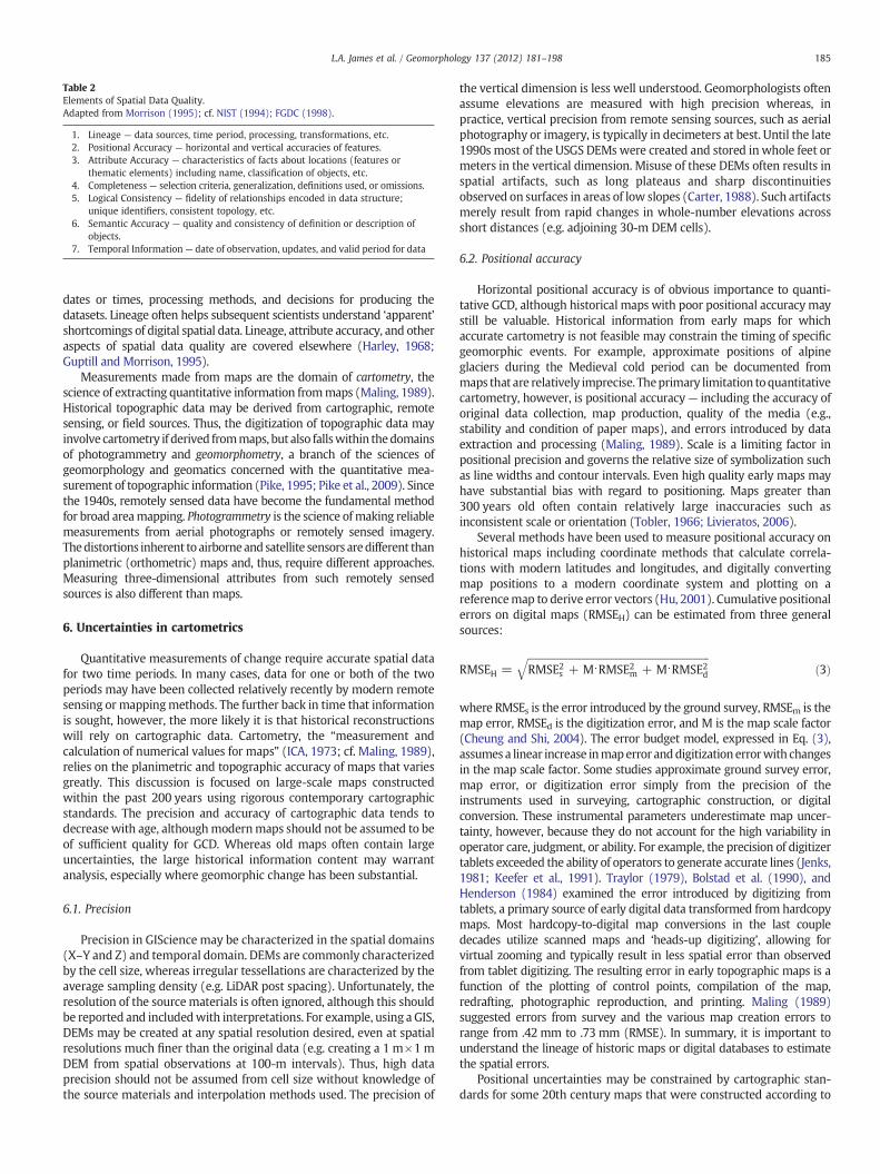
Table 2Elements of Spatial Data Quality.Adapted from Morrison (1995); cf. NIST (1994); FGDC (1998).
1. Lineage — data sources, time period, processing, transformations, etc.2. Positional Accuracy — horizontal and vertical accuracies of features.3. Attribute Accuracy — characteristics of facts about locations (features or
thematic elements) including name, classification of objects, etc.4. Completeness — selection criteria, generalization, definitions used, or omissions.5. Logical Consistency — fidelity of relationships encoded in data structure;
unique identifiers, consistent topology, etc.6. Semantic Accuracy — quality and consistency of definition or description of
objects.7. Temporal Information — date of observation, updates, and valid period for data
185L.A. James et al. / Geomorphology 137 (2012) 181–198
dates or times, processing methods, and decisions for producing thedatasets. Lineage often helps subsequent scientists understand ‘apparent’shortcomings of digital spatial data. Lineage, attribute accuracy, and otheraspects of spatial data quality are covered elsewhere (Harley, 1968;Guptill and Morrison, 1995).
Measurements made from maps are the domain of cartometry, thescience of extracting quantitative information frommaps (Maling, 1989).Historical topographic data may be derived from cartographic, remotesensing, or field sources. Thus, the digitization of topographic data mayinvolve cartometry if derived frommaps, but also fallswithin thedomainsof photogrammetry and geomorphometry, a branch of the sciences ofgeomorphology and geomatics concerned with the quantitative mea-surement of topographic information (Pike, 1995; Pike et al., 2009). Sincethe 1940s, remotely sensed data have become the fundamental methodfor broad areamapping. Photogrammetry is the science ofmaking reliablemeasurements from aerial photographs or remotely sensed imagery.Thedistortions inherent toairborneand satellite sensors aredifferent thanplanimetric (orthometric) maps and, thus, require different approaches.Measuring three-dimensional attributes from such remotely sensedsources is also different than maps.
6. Uncertainties in cartometrics
Quantitative measurements of change require accurate spatial datafor two time periods. In many cases, data for one or both of the twoperiods may have been collected relatively recently by modern remotesensing or mappingmethods. The further back in time that informationis sought, however, the more likely it is that historical reconstructionswill rely on cartographic data. Cartometry, the “measurement andcalculation of numerical values for maps” (ICA, 1973; cf. Maling, 1989),relies on the planimetric and topographic accuracy of maps that variesgreatly. This discussion is focused on large-scale maps constructedwithin the past 200 years using rigorous contemporary cartographicstandards. The precision and accuracy of cartographic data tends todecrease with age, althoughmodernmaps should not be assumed to beof sufficient quality for GCD. Whereas old maps often contain largeuncertainties, the large historical information content may warrantanalysis, especially where geomorphic change has been substantial.
6.1. Precision
Precision in GIScience may be characterized in the spatial domains(X–Y and Z) and temporal domain. DEMs are commonly characterizedby the cell size, whereas irregular tessellations are characterized by theaverage sampling density (e.g. LiDAR post spacing). Unfortunately, theresolution of the sourcematerials is often ignored, although this shouldbe reported and includedwith interpretations. For example, using a GIS,DEMs may be created at any spatial resolution desired, even at spatialresolutions much finer than the original data (e.g. creating a 1 m×1 mDEM from spatial observations at 100-m intervals). Thus, high dataprecision should not be assumed from cell size without knowledge ofthe source materials and interpolation methods used. The precision of
the vertical dimension is less well understood. Geomorphologists oftenassume elevations are measured with high precision whereas, inpractice, vertical precision from remote sensing sources, such as aerialphotography or imagery, is typically in decimeters at best. Until the late1990s most of the USGS DEMswere created and stored in whole feet ormeters in the vertical dimension. Misuse of these DEMs often results inspatial artifacts, such as long plateaus and sharp discontinuitiesobserved on surfaces in areas of low slopes (Carter, 1988). Such artifactsmerely result from rapid changes in whole-number elevations acrossshort distances (e.g. adjoining 30-m DEM cells).
6.2. Positional accuracy
Horizontal positional accuracy is of obvious importance to quanti-tative GCD, although historical maps with poor positional accuracy maystill be valuable. Historical information from early maps for whichaccurate cartometry is not feasible may constrain the timing of specificgeomorphic events. For example, approximate positions of alpineglaciers during the Medieval cold period can be documented frommaps that are relatively imprecise. Theprimary limitation toquantitativecartometry, however, is positional accuracy— including the accuracy oforiginal data collection, map production, quality of the media (e.g.,stability and condition of paper maps), and errors introduced by dataextraction and processing (Maling, 1989). Scale is a limiting factor inpositional precision and governs the relative size of symbolization suchas line widths and contour intervals. Even high quality early maps mayhave substantial bias with regard to positioning. Maps greater than300 years old often contain relatively large inaccuracies such asinconsistent scale or orientation (Tobler, 1966; Livieratos, 2006).
Several methods have been used to measure positional accuracy onhistorical maps including coordinate methods that calculate correla-tions with modern latitudes and longitudes, and digitally convertingmap positions to a modern coordinate system and plotting on areferencemap to derive error vectors (Hu, 2001). Cumulative positionalerrors on digital maps (RMSEH) can be estimated from three generalsources:
RMSEH =ffiffiffiffiffiffiffiffiffiffiffiffiffiffiffiffiffiffiffiffiffiffiffiffiffiffiffiffiffiffiffiffiffiffiffiffiffiffiffiffiffiffiffiffiffiffiffiffiffiffiffiffiffiffiffiffiffiffiffiffiffiffiffiffiffiffiffiffiffiffiffiffiffiffiRMSE2s + M⋅RMSE2m + M⋅RMSE2d
qð3Þ
where RMSEs is the error introduced by the ground survey, RMSEm is themap error, RMSEd is the digitization error, and M is the map scale factor(Cheung and Shi, 2004). The error budget model, expressed in Eq. (3),assumes a linear increase inmaperror anddigitizationerrorwith changesin the map scale factor. Some studies approximate ground survey error,map error, or digitization error simply from the precision of theinstruments used in surveying, cartographic construction, or digitalconversion. These instrumental parameters underestimate map uncer-tainty, however, because they do not account for the high variability inoperator care, judgment, or ability. For example, the precision of digitizertablets exceeded the ability of operators to generate accurate lines (Jenks,1981; Keefer et al., 1991). Traylor (1979), Bolstad et al. (1990), andHenderson (1984) examined the error introduced by digitizing fromtablets, a primary source of early digital data transformed from hardcopymaps. Most hardcopy-to-digital map conversions in the last coupledecades utilize scanned maps and ‘heads-up digitizing’, allowing forvirtual zooming and typically result in less spatial error than observedfrom tablet digitizing. The resulting error in early topographic maps is afunction of the plotting of control points, compilation of the map,redrafting, photographic reproduction, and printing. Maling (1989)suggested errors from survey and the various map creation errors torange from .42 mm to .73 mm (RMSE). In summary, it is important tounderstand the lineage of historic maps or digital databases to estimatethe spatial errors.
Positional uncertainties may be constrained by cartographic stan-dards for some 20th century maps that were constructed according to

186 L.A. James et al. / Geomorphology 137 (2012) 181–198
standards. Error analyses often employ map accuracy standards as thevalue of map error for maps conforming to standards. In the U.S.A.,national cartographic accuracy standards were established in the early1940s (Marsden, 1960) and similar standards have been adoptedinternationally. U.S. National Map Accuracy Standards (NMAS) use anobserved error threshold of 90% for all maps that bear the statement“ThisMapMeetsNationalMapAccuracy Standards.” The error tests that90% of ‘tested’ points on such maps (e.g. U.S. Geological Surveytopographic quadrangles) are within a specified distance of the trueposition (Table 3). Standards formodern geospatial data in theU.S.A. aregiven by the Federal Geographic Data Committee (FGDC 1998).Horizontal standards are stated at the 95% confidence level defined bythe radius of a circle assuming a normal distribution. Similarly, verticalstandards are defined at the 95% confidence level. Of particular interestto geomorphologists are the reference data used in the statistical tests.The ‘tested’ points for such maps meeting NMAS or used in the FGDCNSSDA statistics are “well-defined”, such as street intersections,benchmarks, etc. rather than more ill-defined features such asridgelines, riverine banks, etc. The reliance on well-defined points instatistical tests suggests that the ill-defined features typically of interestto geomorphologists are likely to be less-accurately positioned onmaps.
6.3. Rectification and co-registration
Volumetric changedetection requires that two spatial data sources areco-registered horizontally and vertically with minimal error. Theobjectives of co-registration should recognize differences betweengeodetic coordinate systems related to astronomically orientedgraticules,planimetric references that measure distances or directions betweenlocations of identifiable objects, and elevation references (Laxton, 1976;Blakemore and Harley, 1980; Lloyd and Gilmartin, 1987). Rectification ofhistorical maps and images to a base map or image with preciseplanimetry unleashes the potential for multivariate GIS analysis utilizingancillary spatial data, so referencing to a universal positioning systemhasadvantages.
Prior to the availability and utility of GIS tools, accurate rectification ofhistorical maps and aerial photographs with different scales andprojections or internal distortion often required the use of expensiveand cumbersome optical analogue equipment. Digital corrections ofhistoricmaps began in the 1970s (e.g. Ravenhill andGilg, 1974; Stone andGemmell, 1977). Modern digital rectification methods, available instandard GIS software packages, allowmuch of the systematic positionalerrors to be removed by automated coordinate transfer methods.Historical maps can often be co-registered with other spatial data toovercome scale and projection differences if a set of geographic controlpoints (GCPs) can be identified across bothmaps.Most geomorphologistsare not trained in coordinate transfer methods, however, and may
Table 3Horizontal National Map Accuracy Standards (NMAS) in the United States since 1947.(USGS, 1999).
Scale On mapa On grounda
Factor (inch) (inch) (mm) (m) (ft)
N20,000 1/50 0.0200 0.508 – –
b20,000 1/30 0.0333 0.847 – –
Examples:250,000 1/50 0.0200 0.508 127 417100,000 1/50 0.0200 0.508 50.8 16762,500 1/50 0.0200 0.508 31.8 10424,000 1/50 0.0200 0.508 12.2 40.012,000 1/30 0.0333 0.847 10.2 33.35,000 1/30 0.0333 0.847 4.23 13.9
a No more than 10% of well-defined points can be beyond these error limits. (Thesevalues may be interpreted as the 90% confidence limit with the understanding the NMASdo not assume a specific probability distribution.)
uncritically use the default values in common software packages. Forexample, common procedures require only four GCPs and employ anaffine transformation with ordinary least squares as the default method.Such transformationsmay be adequate to correct for differentmap scalesand orientations, but they are inadequate when the images are based ondifferent projections or contain distortions (Chrisman, 1999). Further-more, planar affine transformations are generally inappropriate for largescale aerial photography. A camera model and appropriate transforma-tion available in softcopy photogrammetric solutions should be used forregistering such remotely sensed data. The polynomial transformationsavailable in a common GIS cannot reproduce the radial distortions, reliefdisplacement, and camera orientation present in an aerial photographwith a central perspective.
Rectification of historical maps and aerial photographs areconventionally done using ground control points (GCPs) that can beidentified on the map and on a reference image, such as buildingcorners, road intersections, or large boulders. A well-distributed set ofGCPs is needed to produce the most accurate rectification. Whereas acamera model is most appropriate for geometric rectification of aerialphotographs derived from a film camera, this approach is foreign tomany geomorphologists. For small geographic areas that cover arelatively small portion of an aerial photograph, simple polynomialtransformations may produce reasonable results. Hughes et al. (2006)examined the sensitivity of aerial photograph rectifications to GCPselection in channel-change studies and provide guidance on thenumber and type of GCPs that are needed. Substantial difficulties maybe encountered in rectifying large-scale historical maps for geomorphicapplications where reliable point features suitable for GCPs are scarce.Cultural features such as road crossings generally stand out on imagery,whereas natural landscapes often lack distinctive point features,especially in heavily vegetated areas. Attempts to use linear featuresdo not generally constrain the rectification in both X and Y, and pointson natural boundaries may migrate through time. For example,attempts to use environmental features such as woodland boundarypatterns are associated with difficulties because of shifting positionsthrough time (Lindsay, 1980), so the stability of landscape features isan important consideration (Lloyd and Gilmartin, 1987). This issue isproblematic for geomorphic studies where cultural features, such asbuildings and roads, may be absent and particularly troublesome forGCD studies where many landscape features have changed.
6.4. Completeness and temporal accuracy of planimetric data
Incomplete coverageonmapscan lead toerrors inhistoric geomorphicreconstructions and distort temporal accuracy such as when geomorphicfeatures appear tochangeonmaps.Apparentgeomorphic changesmaybemisinterpreted from errors of cartographic commission or omissioninherent to the source data. Errors of commission represent the inclusionof anobject thatwasnot present at the timeofmapping. These errorsmayrepresent cartographic blunders such as inclusion without field verifica-tion of a feature shown on an earlier map but no longer present. Errors ofomission occur when a feature was not mapped but was present duringmap data collection. This type of incompleteness may lead to mis-interpretations in the temporal dimension, suchaswhena featureappearsor disappears, or inmeasurement errors, such as computations of erosionor deposition. A notable example in physical geography is the apparentappearance, ‘disappearance’, and reappearance of alpine lakes onsubsequent topographic maps (Butler and Schipke, 1992). Similarly, lackof change may be erroneously inferred from a map that adoptedinformation from a previous map without field verification. Thus, a laterdate on a map does not ensure geomorphic stability unless anindependent fieldmapping surveywas conducted. U.S. Geological Surveytopographic maps have used a magenta color to indicate that features onthepresentmapeditionweremapped fromremotely sensed imagery andnot field surveys. Errors of cartographic omission are commonwhere thearea was incompletely mapped by ground surveys or penetration to the
Fig. 5. Cartographic errors of omission should not be misinterpreted as geomorphic change. (A) Von Schmidt (1859) map shows a single-thread lower Yuba River channel with nosouthern channel. (B) Map showing anastomosed system with small southern channel two years later (Wescoatt, 1861). (C) Later map based on detailed field survey showsanastomosed channel system as former channel positions (Mendell, 1881). These images were manually edited to clarify linework and text from greatly enlarged originals and toremove artifacts introduced by the interpolation process that degrade the graphical quality of lines and lettering.
187L.A. James et al. / Geomorphology 137 (2012) 181–198
ground by remote sensingmethodswas incomplete. For example, studiesof changes in river planform may erroneously record a shift from singlechannel to multithread channel based on an early map that shows only asingle channelwhen additional channels simplywere not included on theearly map. Such errors of cartographic omission were common whenmaps relied entirely on ground surveys (Fig. 5). Time and resources oftenprevented comprehensive mapping of secondary geomorphic featuressuch as headwater streams and gullies (James et al., 2007).
7. Uncertainties in geomorphometry
DEMs have been used for many geomorphic and hydrologic metrics,such as mapping drainage networks (Mark, 1984), steepest slope lines(Chou, 1992), and shallow landslides (Duan and Grant, 2000). TownsendandWalsh (1998) combined DEMs with a variety of remote sensing andGIS data including synthetic aperture radar images to map areas of floodinundation and develop potential flood inundation models for theRoanoke floodplain. Simple rectangular grids (standard DEMs) are notideal for studies of surfaces with abrupt steep surfaces separated by largerelatively flat areas. These surface conditions require high spatialresolutions in the areas of slope changes that result in massive dataredundancy in theflat areas. For example, steep streambanks surroundedby relativelyflatfloodplains call foreitherhighlydensedata setsor theuseof other data models, such as a triangulated irregular network (TIN)supported with breaklines and drainlines (Lane, 2000).
Vertical geodetic positioning differs from vertical positioning relativeto a local relative datumwith an arbitrary elevation. For some cartometricpurposes and for qualitative assessments of change, a relative datummaybe adequate. For quantitative change detection and the construction ofDoDs, however, geodetic control between two data sets may specifyparameters for the vertical co-registration that can prevent systematicbias in elevation changes. Earlymaps often lack accurate geodetic control(or lack documentation), so empirical methods, such as using verticalGCPs in stable locations, may be needed for vertical registration.
Errors in topographic data are important to GCD because they areincorporated in the change-detection analysis and could be misinter-preted as geomorphic change. All DEMs have errors from sampling,measurement, and interpolation, and these will be propagated to
products derived from them such as channel networks (Walker andWillgoose, 1999; Fisher and Tate, 2006). Unfortunately, error propaga-tion is often poorly understood because error sources and the spatialvariation of errors in the source materials, processing, and resultingmaps are seldom documented. Some standard DEM products may notbe well suited for DoD analysis, especially where geomorphic change issubtle (cf. Eq. (2)). Several design specifications of DEMs should beconsidered before they are employed in quantitative GCD, including thescale and contour interval of the source map or imagery, samplinginterval, precision of the base map relative to terrain complexity, andinterpolation method used (Walsh, 1989).
Errors in spatial data are conventionally reported as Circular MapAccuracy Standard (CMAS), RMSE, or more recently as “Accuracy.” Thelatter two statistics are often reported separately for the horizontal andvertical dimensions of the map. RMSE for the entire map, which may bethe only error reported with the data, maymask systematic bias that canbe measured by the mean error or error standard deviation (Fisher andTate, 2006). Knowledge about where errors occur is also of greatimportance, yet the RMSE is devoid of spatial information (Wood andFisher, 1993). Elevation errors refer to specific measurement problemsrelated to differences with reference elevations, while uncertaintyincludes additional doubts in measurement accuracies that are difficultto assess, such as differences introduced by interpolation or rescaling(Fisher and Tate, 2006). Vertical errors are affected by accuracies of thereference data and by the number and spatial distribution of controlpoints used for geometric rectifications or interpolations (Li, 1991).Estimates of vertical accuracies in the reference data may be constrainedby vertical map accuracy standards for maps conforming to standards. Inthe U.S.A., NMAS require at least 90% of points to have elevations thatdiffer by no more than 1/2 the contour interval (USGS, 1999).
Vertical errors in DEMs can be attributable to poor verticalregistration, improper geodetic control, errors inherent to topographicdata used, or errors introduced by horizontal error. These errors arecompounded in the generation of vertical change data (e.g., DoDs).Vertical errors introduced by horizontal error are particularly importantin geomorphic studies because they are common, can be large inmagnitude, and are associated with steep slopes, so they often occur atcritical locations such as terrace or fault scarps, stream banks, or dune
188 L.A. James et al. / Geomorphology 137 (2012) 181–198
faces. The inter-dependency between vertical and horizontal error iswell known and has interesting implications regarding the effects ofDEM grid-cell size that influence variability in DEMs. Vertical errorscaused by horizontal offsets in a map can be estimated as a function oflocal slopes and the horizontal errors (Maling, 1989, p. 154; Hodgsonet al., 2005):
εZH = εH tan α ð4Þ
where εZH is the elevation error caused by horizontal offsets on a slopingsurface, εH is the horizontal error, andα is the local slope. Becausemostgeomorphic slopes are less than 45°, most vertical errors caused byhorizontal displacement, α, will be less than the horizontal displace-ment, εH (Maling, 1989). For slopes N45°, however, errors recorded bythis metric increase rapidly with slope, and go to infinity in the limit asslope approaches 90°. Thus, it may be prudent to constrain themaximum error calculated by this method to no more than the reliefof local features. A map of estimated vertical errors, attributable to aconstant worst-case horizontal offset, can be computed for DEMs bycomputing slopes between cells and utilizing the horizontal RMSEH toestimate the horizontal offset error of individual grid cells:
RMSEZij = RMSEH tan Sij ð5Þ
where RMSEZij is the vertical error in a cell of the error grid caused by thehorizontal offset and slope,RMSEH is the horizontal error for themap, andSij is the slope of a grid cell in the slope grid. The vertical error resultingfrom a horizontal error is directionally dependent — a horizontal errorparallel to a slope will have no resulting vertical error. The fundamentalEq. (5) can be extended by Monte Carlo simulation modeling toincorporate random horizontal error directions with a known (meanand standard deviation) slope distribution (Hodgson and Bresnahan,2004):
RMSEZ = a1� tan meanslope
� ��RMSEH� �
+ a2�σslope�RMSEH
� �ð6Þ
where a1 and a2 are constants for the population of slopes in a study area.
7.1. Interpolating DEMs from topographic point, contour, and TIN data
DEMs may be generated from topographic information based onfield surveys, topographic maps, stereo pairs of aerial photographs, orother remotely sensed data (Hutchinson and Gallant, 2000; Lane, 2000;Jensen, 2007; Nelson et al., 2009). An important source of uncertainty ingriddedDEMs is themethodof interpolationused togenerate a lattice ofelevation points from other topographic data structures. Topographicdata may be stored and displayed as contour lines, profiles, DEMs, TINs,or clusters of points. The structure, completeness, and planimetric andtopographic accuracyof thedata should be considered in the selectionofan appropriate interpolation method and grid-cell size. Interpolation ofcontours can be done using automated procedures available on mostcommercialGIS software packages by a varietyof interpolationmethods(Carrara et al., 1997). Many studies have documented contour-to-gridinterpolation algorithms including the addition of ancillary data (e.g.drainlines or hypsography) and the resulting quality of DEMs. Animproper method can introduce artifacts in the DEM. Guth (1999)evaluated USGS DEMs that were based on a contour-to-grid algorithmand found systematic high (and corresponding low) frequencies ofelevations (“contour line ghosts”) with values peaking at the contourline elevations. For example, micro-topographic ‘stepping’ can beintroduced in low-relief areas by interpolating between contour linesalong north–south and east–west trend lines rather than following flowlines perpendicular to contours (Pelletier, 2008). Such early directionalproblems with USGS DEM production led to the adoption of the U.S.Forest Service's Linetrace algorithm that utilized 8-directional interpo-
lation lines and later, the incorporation of hydrography in DEM Level 2production.
Interpolations of DEMs may be accomplished by several automatedmethods including kriging or inverse distance weighting (IDW). Forexample, a controlled experiment, comparing DEM interpolations bykriging, variations of IDW, and from contours, found that vertical errors(RMSEZ) in DEMs interpolated by kriging were consistently smallest(Defourny et al., 1999). Surprisingly, errors in the DEM constructed usingIDW with a short search radius were comparable to errors in the TINsurface. DEMs created with IDW using a larger search radius were notviable. Errors inDEMsgenerated fromcontour linesweregreat (Defournyet al., 1999), and suggest that DEMs generated from topographic mapswill have larger uncertainties introduced by interpolation than otherDEMs.
7.2. High-resolution DEMS
One way to reduce vertical errors caused by horizontal offsets is togenerate DEMs with a high spatial resolution and reduced horizontalerror. High-resolution topographic data from airborne laser scanning(LiDAR) have been used to generate DEMs for GCD in a variety ofapplications. The common success of these applications has resulted in acall for a new generation of topographic data collection (Stoker et al.,2008). Rapid advancements in LiDAR data quality and processingcapabilities are a boon to geomorphic studies involving large-scaleimagery, particularly in low-gradient environments, and provide anexcellent modern base for historical change studies. LiDAR-derivedDEMs are not without problems, however, and several studies havemeasured uncertainties associated with these data (Hodgson et al.,2003; 2005; Hodgson and Bresnahan, 2004; James et al., 2007; Raberet al., 2007; Aguilar andMills, 2008;Wheaton et al., 2009; Aguilar et al.,2010). Moreover, simply increasing mean point densities does notensure significantly improved vertical accuracy (García-Quijano et al.,2008). Airborne LiDAR has potential for penetrating through modest orleaf-off canopy but still does not penetrate well through thicklyvegetated (or other surface cover) environments. For example, relativelyflat floodplains with thin vegetation may have relatively small verticalerrors in airborne LiDAR bare-earth point data, but errors increase ondensely wooded slopes such as river banks (Cobby et al., 2001).
7.3. Completeness of topographic information
For cartographic measurements and feature mapping that arerestricted to certain areas; e.g., channel or dune boundaries, accuraciesof elevation data need only to be assured for those locations. Forconstruction of DEMs, however, accuracymust be assured over the entirearea to be included in themodel. Thismay be problematic with the use ofsome old topographic maps if the efforts of field surveys were non-uniformover the areaof themap.Greater attentionmayhavebeenpaid toaccessible areas, to prominent topographic features, or to areas of interest,than to heavily vegetated or inaccessible areas away from the studyobjective. For example, a historic map of fortifications around a frontiertown may be based on precise surveys around the fort but mapping of aheavily wooded river channel at the base of the hill may be approximateand incomplete. In cases of contour incompleteness, the resulting DoDsmay indicate apparent changes thatwere not real. If the early topographicmap failed to include an area where later high-resolution data measuredtopographic features, the lack of contours will be interpreted as flat orfeatureless terrain and the DoD will erroneously show changes at thelocationsof the features. For example, positive relief features suchasbeachridgesordunesmissing fromanearlymapbutmapped laterwill appear asdeposits on theDoD. The analyst interpreting the change detectionmodelshould consider the possibility that elevation differences on the DoDmayreflect differences in map completeness rather than actual change. Suchconcerns are less of an issue for modern maps using remote sensing dataand adhering to accuracy standards.

189L.A. James et al. / Geomorphology 137 (2012) 181–198
8. Uncertainties associated with DEM differencing
Uncertainties that arise from data acquisition, recording, and post-processing may be larger than actual geomorphic change, and construc-tionofDoDs compounds theseuncertainties. TheDoDmethodmaynotbeappropriate where real geomorphic changes are small and uncertaintiesare large. This question of appropriate application is especially relevant tohistorical reconstructions using data such as historical maps that mayhave large errors. Cartographic-based applications of theDoDmethod arebest reserved for cases where relatively accurate cartographic data areavailable and geomorphic changehas been considerable. An evaluation ofthe uncertainty of a DoD should consider three steps (Wheaton et al.,2009):
1) quantification of uncertainty in each individual DEM,2) propagation of these uncertainties into the DoD, and3) an assessment of the importance of the propagated uncertainty.
The first step was covered under cartometric and geomorphometricuncertainties and can also be shown by an evaluation of the accuracyand precision of the data and procedures used to generate DEMs. Someresearchers recommend that values of change be filtered by setting tozero values that are small relative to errors. Wheaton et al. (2009)suggested the use of a critical threshold, t, for screening the changemodel based on the ratio of observed elevation change to error:
tij = jZ2ij–Z1ij j = εDoD ð7Þ
where |Z2ij−Z1ij| is the absolute value of the DoD and εDoD is thecomposite error associated with the DoD propagated by the two DEMs:
εDoD =ffiffiffiffiffiffiffiffiffiffiffiffiffiffiffiffiffiffiffiffiffiε21ij + ε22ij
qð8Þ
where ε1ij and ε2ij are the vertical errors in cells of the early and lateDEMs,respectively. They recommendusing a critical threshold (e.g.α=95%) fort values to filter out changes in the DoD that are not significantly differentthan the errors. This ratio has intuitive appeal because it is similar to asignal-to-noise ratio that measures the magnitude observed changes inthe DoD (real change plus uncertainties) relative to uncertainties. Ifthe cumulative error (εDoD) is normally distributed and based on a prob-ability distribution, then Eq. (7) is similar to the equation for computing az-score, and the t-valuewould reflect the confidence that the changewasan actual change. Where topographic change is large and uncertainty issmall (εDoD), values of |Z2ij−Z1ij| and t values will be high, the likelihoodof variability being generated primarily by errorwill be small, and the cellwill not be filtered from the DoD model. The difficulty in applying thismethod is computing the actual errors for the individual DEM grid cells.
The process of filtering out all cells with small change should beundertakenwith caution, because filteringmay eliminate extensive realchanges that are cumulatively important. In some cases, small verticalchanges of the same sign may be widespread and comprise a largeproportion of the sediment budget. For example, floodplain sedimen-tation by overbank processes may be thin but constitute a large volumeof sediment. If errors can be assumed to be normally distributed, thedistribution of small changes can be tested for symmetry around themean to ensure against bias in the filtration process.
9. Examples of change detection in fluvial processes
Three case studies are presented to demonstrate the use of historicalmaps in conjunction with LiDAR or photogrammetric data to produceDoDs. Thefirst example is a gully system in the upper Piedmont of SouthCarolina. The next two examples are large rivers and floodplains inCalifornia where historical sedimentation and channel change wereextreme. Detailed historical topographic maps and modern high-resolution remote sensing data are available for all three sites. High-resolution time-sequential DEM pairs were generated for each area by
digitizing early topographic data from topographic maps and differenc-ing them with modern high-resolution topographic data (Eq. (1)) toproduce high-resolution DoDs. Each site presented different limitationsand challenges to theDoDmethod, so these studies provide a diverse setof examples of the method applied to fluvial landforms.
10. Cox gully
Gully erosion poses a serious threat to environmental systems bydamaging productive lands, increasing flood magnitudes, and deliv-ering non-point-source pollution. They generate dense, more efficientdrainage networks, raise flood stages as a result of lowland channelfilling, and degrade water quality by generating non-point-source(NPS) pollution. Gullies in the Piedmont region of the southeasternU.S.A. were highly active in the early 20th century because of forestclearance, lack of conservation measures, and intense rainfalls. TheUpper Piedmont region is characterized by moderate local relief, intowhich gully incision generates a striking vertical relief along sidewallsand headwalls. Gullies in this area were studied carefully during theearly stages of soil conservation research in the United States (Irelandet al., 1939). In the 1930s, agriculture in the southern Piedmont regiondeclined rapidly, soil conservation measures were introduced,reforestation ensued, and many gullies stabilized. Little study hasbeen done of these systems sinceWorldWar II because of the need forground-based surveys, and it is often assumed that gullies are nolonger active. The first example of DoD analysis is focused on the CoxGully system, which was surveyed in 1938 (Ireland et al., 1939).
10.1. Map and LiDAR processing
A preliminary DoD for the Cox gully from 1938 to 2004 wasdeveloped using the historical map (Ireland et al., 1939) and airborneLiDAR data collected for Spartanburg County in August, 2004 for theSouth Carolina Flood Map Modernization Project. Topographic datawith sufficient resolution to map gullies in this region were rare priorto the advent of airborne LiDAR because photogrammetric analysis isrestricted by thick vegetation. Fortuitously, detailed topographicsurveys, mapping, cross-sections, longitudinal profiles, and strati-graphic analysis of several active gully systems in Spartanburg County,South Carolina were conducted in the late 1930s (Ireland et al., 1939).Modern LiDAR mapping techniques have proven to be effective inmapping gully systems under forest canopy in the region, althoughLiDAR bare-Earth data from standard processing can produceinaccurate cross-section morphologies of gullies (James et al., 2007).Several gullies studied by Ireland et al. (1939) were revisited in thefield from 2000 to 2004. The Cox gully was singled out for a detailedstudy (Kolomechuk, 2001) that was followed by field surveys tomeasure topographic changes since the Ireland et al. (1939) surveys.
The 1939 map was scanned and preprocessed to remove specklingand shading (Fig. 6). Use of conventional ground control points (GCPs)formap registrationwas severely limitedby the lackofdistinctive pointson the historic map. This is a common problem with historical mapanalysis that may limit the accuracy of reconstructions. Instead,registration was based on a combination of three types of registrationpoints on the map and the digital orthophoto quarterquad (DOQQ):(1) two conventional GCPs distinctly identifiable on both images, (2) 15synthetic GCPs were generated on an orthogonal grid of points, and(3) 35 approximately located GCPs at critical locations on the map toensure that the 1939 gully rims did not extend beyond the 2004 rims.The synthetic gridwas generated by using the graphical scale bar on the1939 map to space points along the centerline of a road and onperpendiculars from the road. The same grid was constructed on thereference image using identical spacings and bearings. The advantage ofthis method is that it allows the map to be approximately registered tothe DOQQ in spite of the lack of uniquely identifiable GCPs. Two keydisadvantages of this method are that the synthetic GCPs are not based

Fig. 6. Cox Gully, Spartanburg, South Carolina. Rectified excerpt from topographic map surveyed in 1938 by Ireland et al. (1939).
190 L.A. James et al. / Geomorphology 137 (2012) 181–198
on true positions so they may force map deformation and the accuracyof the registration cannot be quantified. The RMSE reported by theregistration (0.27 m) represents only the success of fitting the map totheGCPs. Becausemost of theGCPswere simulated or approximate, thismetric grossly underestimates errors and should not be used as anindicator of the planimetric accuracy of the resulting map. The generalorientation of the gully systemon the resultingmapwas validatedusingGPS points collected along the rim of the modern gully.
LiDAR data for Spartanburg County were collected by airbornescanning in three flights April 5, 6, 7, 2004 by Woolpert, LLP, for usecompatible with developing 0.6-m (2-ft) contours. Counting the bareEarth points in a 14 ha rectangle around the gully yielded a mean pointdensity of 0.10 pts/m2 which converts dimensionally to a mean pointspacing of 3.2 m/pt. Unfortunately, the bare Earth data in the study area– as delivered – have a non-uniform spatial distribution that is stronglybiased towards clearings. The gullies are heavily wooded, so pointdensities within the gullies are sparse. The point cloud is available andfuture analysis will ultimately re-process a new bare Earth data set. Forthis preliminary study, the existing points were interpolated to a70×70-cm DEM using inverse distance weighting (IDW) based on 12points in a variable search radius. This interpolationworkedwell for theinner gullies, although the resulting DEM has a stair-stepping artifactthat propagated into the DoD analysis. The 2004 DEM from the IDW
Fig. 7. Cox Gully cross section changes based on field surveys in 1938 and 2001 (seeFig. 8 for locations). Section D12 is representative of main-stem gully sections that filledandwidened. Gully E did not exist in 1938 and represents post-1939 gully erosion N4 mdeep and 9 m wide.
Fig. 8. Cox Gully DoD map with gully rims derived from contours for both periods.(A) Changemodel shows erosion by widening of sidewalls and deposition in gully bottoms.Two small gullies on south side were filled after 1938 as was the upper half of the largeeastern gully, but the lower half of the eastern gully was not detected by LiDAR owing todense canopy and backfilling. (B) Close-up of north branch with 1938 contours over DoDchangemodel showingheadward extension andmore than 2mof deposition on gullyfloorsincluding deep fill in former plunge pool (center of image). Northeast gully branch withcross-section ‘E’ did not exist in 1938 and was surveyed with a total station in 2001 (Fig. 7).
191L.A. James et al. / Geomorphology 137 (2012) 181–198
interpolation was used to generate a contour map that was morerealistic than a contour map generated directly from a TIN of LiDARpoints; i.e., overall contour patterns were similar but the IDW-derivedcontours were smoother and lacked the angularity of TIN-derivedcontours. The resulting contour map and DEM of gullies conformsapproximately to contemporary topographic cross sections and otherfield observations (Fig. 7). A DEM of difference (DoD) was constructedby differencing the 1939 and 2004 DEMs (Fig. 8A).
In spite of large uncertainties arising from poor 1939map registrationand low point densities of LiDAR data within gullies, several importantgeomorphic changesandprocessescanbe identified fromthispreliminarychange model in addition to guidance towards future methodologicalimprovements. LiDAR data detected but underestimated the depth of anewnortheasternbranchof theCoxGully system. Thisunderestimationofthe depths of V-shaped gullies and rounding of gully rims typical of ‘off-the-shelf’ LiDAR bare-Earth point clouds derived from landscapes underforest canopy in this regionbecauseof the lowdensityof bare-Earthpointswithingullies (Jameset al., 2007).Hopefully, themappingof forestedgullymorphologies can be improved by careful reprocessing of the point-clouddata testing multiple methods with special focus in the vicinity of gullies.Detection of the new gully branch indicates that substantial erosionoccurred after the 1938 survey and that these features can be detectedusing LiDAR data. In addition, the GCD using historical maps revealsseveral local-scale geomorphic processes. For example, main gullies filledand widened in conformance with common gully evolutionary processes(Ireland et al., 1939; James et al., 2007). Moreover, a pocket of fill N3 mdeep in theheadof themain1939northgully indicates thepresenceof theformer plunge pool (Fig. 8B). Comparisons of 1939 and 2004 gully crosssections show substantial filling in the lower gully in that period (Fig. 7).Filling had begun in the lower gully prior to 1939 as was shown by corestratigraphy and photographs at that time (Ireland et al., 1939). The CoxGully DoD, therefore, provides guidance for a sediment coring program ofthe gully floor.
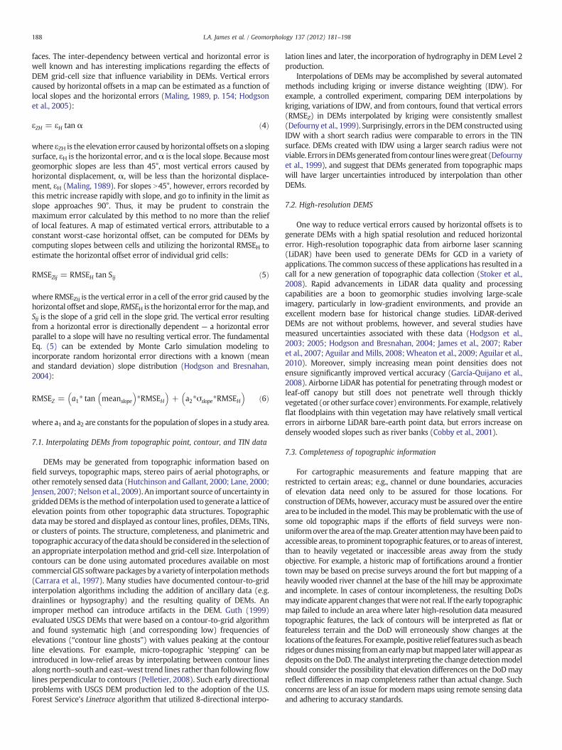
Fig. 9. Excerpt from 1909 Feather River map downstream of Shanghai Bend. Digitalbathymetry interpolated from depths along 1909 channel cross section survey points.Vertices sampled from the bathymetric and terrestrial contours were used to interpolate aTIN.(Adapted fromMegison, 2008).
11. Feather River at Shanghai Bend
This example examines geomorphic changes in a 1.8-kmreach of thelower Feather River from1909 to 1999. Prior to 1909, the river had beenaffected by sedimentation following hydraulic mining and a consider-able amount of channel and floodplain engineering, including leveesand channel dredging (James et al., 2009). At the time of the 1909survey, channels in the area were avulsing from positions where theyhad been for at least 50 years to new channelized positions fromwherethey subsequently migrated to the present configuration formingShanghai Bend. Thus, this is a case of exceptional geomorphic changerather than a randomly selected site.
A modern (1999) DEM for the floodplain around Shanghai Bendwas extracted from an extensive data set generated by airborne LiDARas part of a study designed to compare LiDAR and photogrammetry(Stonestreet and Lee, 2000; Towill, 2006). LiDAR data were acquiredby EarthData Aviation using a fixed-wing aircraft flying between 2440and 2740 m above mean terrain, on March 27 and 28, 1999, using anAeroScan system with a scan rate of 50 Hz. The aerial survey wasperformed with a Phalanx inertial measurement unit (IMU) and adual frequency GPS receiver, in conjunction with a mobile kinematicGPS survey. The LiDAR mission was designed to acquire data with ahorizontal accuracy of 1 m RMSE and a vertical accuracy of 15 to20 cm RMSE. The resulting points have reported mean postingsvarying from 1.5 to 6.1 m and, based on comparing points inoverlapping areas between flight lines, a vertical accuracy of 19.3cm RMSE (Towill, 2006). A third party (Douglas Allen written comm.)merged the data with channel bathymetry data collected in 1999 by ahydrographic boat survey using a real-time and post-processedkinematic GPS survey, a fathometer, and sonar transducer to meetthe requirements of a Class 2 Hydrographic Survey (Ayres, 2003). The
merged 1999 data set was interpolated to a 3×3 m DEM using krigingwith a linear model.
A set of large-scale map sheets, produced from floodplaintopographic surveys in 1909 (CDC, 1912), was used to generate a1909 DEM for DoD analysis (Megison, 2008). The 1909 maps did notinclude channel bathymetry, but they did include frequent crosssections showing channel depths as a set of closely-spaced pointsacross the channel. These point depths were associated with low-water elevations printed at several locations on the map. They wereconverted to point channel-bottom elevations and used to manuallyinterpolate bathymetric contour lines that were combined with theterrestrial contours (Fig. 9). Contours were given a slight longitudinalorientation to simulate longitudinal or lingoid bars common to sandbedded streams (as opposed to random as automated proceduresmaygenerate or transverse as may occur in some other environments).
Points extracted from the 1909 contours (including bathymetry),field survey points, and low-water edge contours were used in a spatialinterpolation to a 3×3 m grid co-registered with the 1999 LiDAR DEM.Four methods of interpolation were tested on the Shanghai Benddataset: kriging, IDW, TIN to raster, and Topogrid, a tool in the ArcGISSpatial Analyst toolbox (©ESRI, Corp.). For kriging and IDW, pointlocations and elevation valueswere extracted from the contour linedataat a 3-m spacing and produced cross-validated vertical RMSEs of0.355 m and 0.420 m, respectively. In spite of the lowRMSEvalues, bothmethods created a stepping effect on the floodplain where a gradualchange in elevation is more realistic. TopoGrid uses a spline function togenerate a hydrologically correct DEM from contour-line data byaccentuating topographic variation in areas lacking elevation data. The1909 Shanghai Bend floodplain map has broad areas of sparse data.

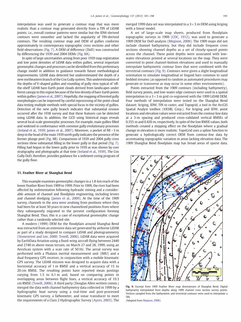
Fig. 10. Shanghai Bend 1909 DEM constructed from CDC (1912) topographic map (in background).(Adapted from Megison, 2008).
192 L.A. James et al. / Geomorphology 137 (2012) 181–198
TopoGrid modeled elevations in these areas as unrealistic peaks ortroughs, so this method was dropped from further analysis. The TINmethod allows input of points and contour lines. Contour lines wereinput as soft breaklines, water-surface boundaries as hard breaklines,and survey points asmass points. The TIN-derivedDEMwas selected forfurther study because of the lack of stepping and realistic gradual slopeson such features as point bars.
The resulting 1909 DEM shows the channel in the initial processof an avulsion from an early eastern position into a dredged channelalong the west levee (Fig. 10). Interestingly, a large natural levee hadalready formed along the east bank of the new channel, whichpresumably reflects the high loads of mining sediment carried bythe river at this time (James et al., 2009). Eliza Bend, the old, high-amplitudemeander to the northeast, was cut off by this avulsion, locallysteepening the channel, and providing excess hydraulic energy thatultimately led to lateral channel migration and the formation ShanghaiBend at this site.
The 1909 and 1999 DEMs were vertically registered by anempirical test that compared elevations of stable 1906 and 1999surfaces outside of levees along cross sections generated from bothdata sets and validated by comparisons with contemporaneous(1909) cross-section surveys and profiles extracted from the 1999LiDAR data. The vertical datum on the 1909 map was assumed to bethe United States Engineering Datum whereas the 1999 LiDAR-basedDEM was referenced to the NGVD29. Tests confirmed a −0.76 mvertical offset between the DEMs and this adjustment was made tobring the 1909 elevations to NGVD29. The two DEMs were thendifferenced to produce a DoD that reveals net changes integrated overa period of 90 years (Fig. 11). These GCD models illustrate spatialpatterns of sediment reworking in a very active fluvial system. Lightshaded areas on the models represent net sediment deposition. Zonesofmaximum sedimentation occurred as channel fill near the top of theDoD where the thalweg of the former channel filled up to 7.9 m.Downstream, the former thalweg filled with up to 6 or 7 m ofsediment in narrow strips. A 300-m stretch of the former canal alongthe west levee is now filled with 6−6.5 m of sediment. Thesesediment deposits are important because of the high concentrations
of total mercury associated with the hydraulic mining sediment in thesystem (James et al., 2009). The natural levee, showing in 1909(Fig. 10), is not present in 1999, which suggests that Shanghai Bendformed by lateral migration to the east rather than by avulsion. Thisinterpretation is supported by the presence of a large gravel point baron the inner bend. The large rectangular eroded areas in the center ofthe DoD are lagoons for a sewage treatment plant. The dark shadedareas of Fig. 11 indicate erosion depths up to 14.4 m primarily withinthe modern channel. The deepest erosion occurred in the southernpart of Shanghai Bend along the outer cut bank at the southern end ofthemap. Other areas of deep erosion include the point bar – especiallyin a chute – and along the lower banks of the old channel where, thenatural levee is now gone, possibly because of the migration of thesecondary channel. Draping a 1952 aerial photograph over the DoDbrings out the geomorphic context of the changes (Fig. 11C). Thisdiffers from draping over a standard DEM in that zones of depositionare shown in positive relief even where the present topography maybe low. For example, the deeply alluviated paleochannels are shownas ridges. The light tonality indicates relatively recent sedimentationat the time of the photograph (e.g., on-going channel filling and point-bar construction in 1952).
11.1. Vertical uncertainties in the Shanghai Bend DoD
An analysis of vertical uncertainty in the 1909 and 1999 ShanghaiBend DEMs was conducted based on an error budget approach(Megison, 2008). Some uncertainty values were assumed to be uniformacross the surface whereas others were associated with spatiallydistributed uncertainty grids (Table 4). Horizontal accuracies werecomputed and applied to the vertical assessment, as demonstrated herewith the 1909 data. Horizontal accuracies were computed as a functionof two factors. Cartographic uncertainty (RMSECart) accounts forinaccuracies, such as line work, and was set to a uniform value basedon the fair drawing error of less than 0.5 mm (Maling, 1989) orapproximately 4.8 m on the ground at the 1909 map scale of 1:9600.Horizontal map registration uncertainties (RMSEReg) are potentiallyhigh on large paper sheets such as the 1909maps. To estimate RMSEReg,

Fig. 11. DoD for Feather River floodplain at Shanghai Bend, 1909 to 1999. (A) DoD mapshowing up to 14.4 mof erosion (dark shades) alongmodern Shanghai Bend andup to 7.9 mof fill (light shades) in abandoned 1909 channels along the eastern levee and the canalcrossing the bend along the west levee. (Adapted from Megison, 2008) (B) Oblique viewupstream of DoD showing abandoned channel deposition and erosion of main channel.(C) 1952 aerial photograph draped over oblique view of DoD. (B and C are at 8× verticalexaggeration).
Table 4Uncertainties used to compute error budget for 1909 data at Shanghai Bend.
Source of uncertainty Value or range Symbol Comment
Map (mm) Ground (m)
Uniform values:Horizontal registration 0.65 6.26 RMSEREG PlanimetricCartographic 0.50 4.80 RMSECART PlanimetricInherent horizontal 0.82 7.89 RMSEH PlanimetricMap interpolation to DEM – 0.765 RMSEZInt VerticalContour data – 0.185 RMSEZCont Vertical
Gridded values:Vertical by horizontaloffsets
– 0–9.30 RMSEZH.ij Vertical range
Total vertical Uncertainty – 0.787–9.33 RMSEZij Vertical rangeSlope – 0–50°* α Range of angles
*Slope values are not uncertainties but control the uncertainties of RMSEZHij.
193L.A. James et al. / Geomorphology 137 (2012) 181–198
66measurements along a railroad on the 1909 and 1999 reference datawere used to compute one-dimensional RMSE for the 1909 map:
RMSE1D =ffiffiffiffiffiffiffiffiffiffiffiffiffiffiffiffiffiffiffiffiffiffiffiffiffiffiffiffiffiffiffiffiffiffiffiffiffiffiffiffiffi∑ di−di + 1
� �2 = nq
ð9Þ
where di−di+1 is the horizontal difference between the 1909 and1999 measurements. Assuming the error along this one dimensionwas the same in the orthogonal direction, this RMSE1D was convertedto a two-dimensional RMSE for horizontal map registration uncer-tainty (RMSEReg):
RMSEReg =ffiffiffiffiffiffiffiffiffiffiffiffiffiffiffiffiffiffiffiffiffiffiffi2�RMSE21D
qð10Þ
where RMSEReg, the potential error inX andY. This uncertainty, a uniformvalue of 6.26 m on the ground (Table 4), is based onmeasurements fromthe 1909 to 1999 digital data, so it presumably includes all digitization,map compilation, reproduction, and registration uncertainties. Assumingthe error sources are independent, cumulative horizontal uncertaintieswere estimated to be 7.89 m from cartographic and registrationinaccuracies:
RMSEH =ffiffiffiffiffiffiffiffiffiffiffiffiffiffiffiffiffiffiffiffiffiffiffiffiffiffiffiffiffiffiffiffiffiffiffiffiffiffiffiffiffiffiffiffiffiRMSE2Cart + RMSE2Reg
qð11Þ
where RMSEH is the horizontal uncertainty that is assumed uniformacross the map.
Vertical uncertainties were computed from three factors: inaccu-racies introduced by horizontal offset, contour lines, and interpola-tions. Horizontal offsets were assumed constant and equal to RMSEHthat was combined with a 1909 slope grid, Sij, to compute a map ofvertical uncertainties caused by horizontal offset (RMSEZHij) (cf.Eq. (5)). Uncertainties introduced by vertical errors (i.e. as exhibitedin the contour lines) were estimated based on U.S. NationalCartographic Accuracy Standards; i.e., 90% of point elevations differsno more than one half of the contour interval. Although these mapswere generated prior to establishment of the Standards, they wereproduced under the supervision of the California Debris Commission,an affiliate of the War Department (now U.S. Army Corps ofEngineers), presumably using equally high accurate and precisecartographic methods. The interval for the CDC (1912) topographicmaps is 0.610 m (2 ft), so one half of the interval is 0.305 m. Weassumed that the 1912 map met the one-half contour intervalthreshold and that less than 10% of the points on contour lines havevertical errors exceeding 0.305 m. To convert the one-dimensional90% confidence level to a 68% confidence level, 0.305 m was dividedby 1.645, resulting in a uniformly distributed contour uncertainty of0.185 m across the 1909 DEM. Interpolation uncertainties wereestimated empirically. The interpolation error was measured at acompanion study site downstream and applied to the Shanghai Bendsite. Vertices of the TIN along contours, combined with other knownpoint features, were treated as ‘known’ z-values and compared with
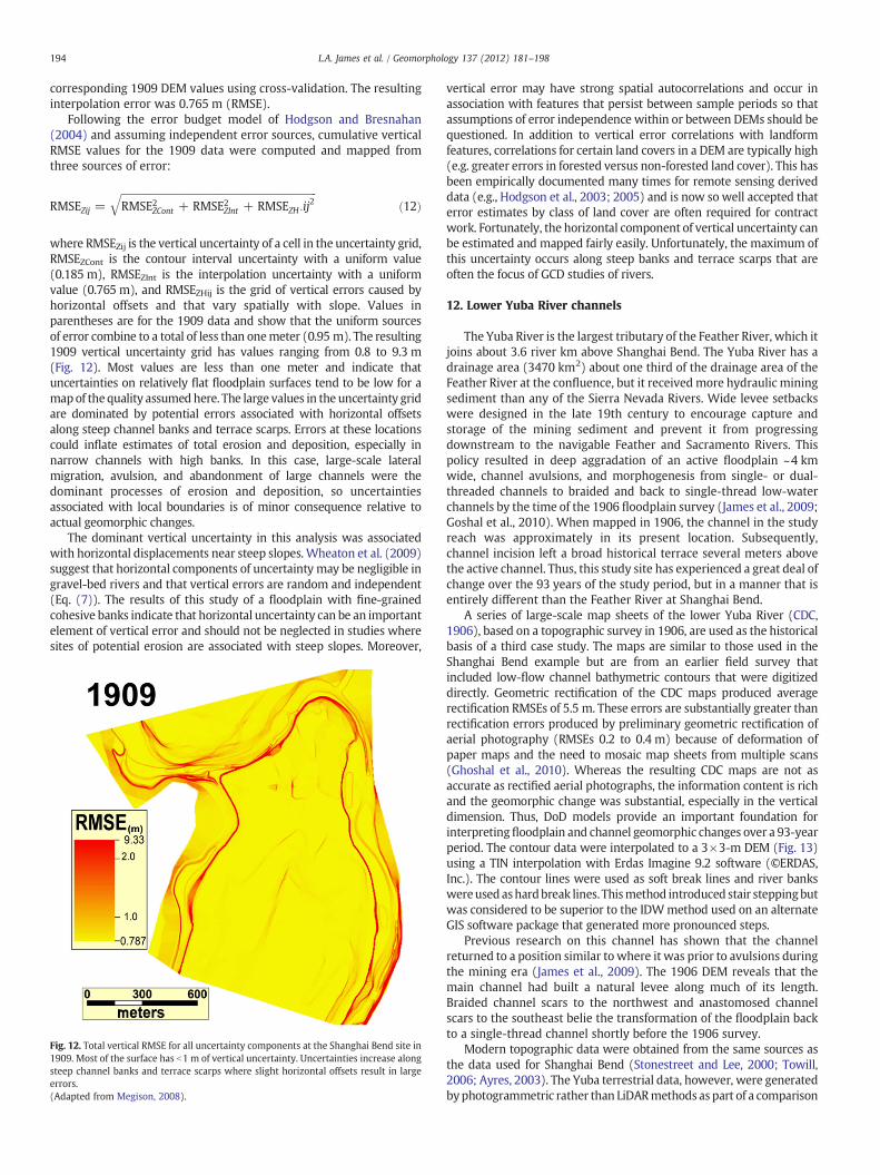
194 L.A. James et al. / Geomorphology 137 (2012) 181–198
corresponding 1909 DEM values using cross-validation. The resultinginterpolation error was 0.765 m (RMSE).
Following the error budget model of Hodgson and Bresnahan(2004) and assuming independent error sources, cumulative verticalRMSE values for the 1909 data were computed and mapped fromthree sources of error:
RMSEZij =ffiffiffiffiffiffiffiffiffiffiffiffiffiffiffiffiffiffiffiffiffiffiffiffiffiffiffiffiffiffiffiffiffiffiffiffiffiffiffiffiffiffiffiffiffiffiffiffiffiffiffiffiffiffiffiffiffiffiffiffiffiffiffiffiffiffiffiffiffiffiffiffiffiffiffiffiffiffiffiffiRMSE2ZCont + RMSE2ZInt + RMSEZH :ij
2q
ð12Þ
where RMSEZij is the vertical uncertainty of a cell in the uncertainty grid,RMSEZCont is the contour interval uncertainty with a uniform value(0.185 m), RMSEZInt is the interpolation uncertainty with a uniformvalue (0.765 m), and RMSEZHij is the grid of vertical errors caused byhorizontal offsets and that vary spatially with slope. Values inparentheses are for the 1909 data and show that the uniform sourcesof error combine to a total of less than onemeter (0.95 m). The resulting1909 vertical uncertainty grid has values ranging from 0.8 to 9.3 m(Fig. 12). Most values are less than one meter and indicate thatuncertainties on relatively flat floodplain surfaces tend to be low for amapof thequality assumedhere. The large values in the uncertainty gridare dominated by potential errors associated with horizontal offsetsalong steep channel banks and terrace scarps. Errors at these locationscould inflate estimates of total erosion and deposition, especially innarrow channels with high banks. In this case, large-scale lateralmigration, avulsion, and abandonment of large channels were thedominant processes of erosion and deposition, so uncertaintiesassociated with local boundaries is of minor consequence relative toactual geomorphic changes.
The dominant vertical uncertainty in this analysis was associatedwith horizontal displacements near steep slopes. Wheaton et al. (2009)suggest that horizontal components of uncertainty may be negligible ingravel-bed rivers and that vertical errors are random and independent(Eq. (7)). The results of this study of a floodplain with fine-grainedcohesive banks indicate that horizontal uncertainty can be an importantelement of vertical error and should not be neglected in studies wheresites of potential erosion are associated with steep slopes. Moreover,
Fig. 12. Total vertical RMSE for all uncertainty components at the Shanghai Bend site in1909. Most of the surface has b1 m of vertical uncertainty. Uncertainties increase alongsteep channel banks and terrace scarps where slight horizontal offsets result in largeerrors.(Adapted from Megison, 2008).
vertical error may have strong spatial autocorrelations and occur inassociation with features that persist between sample periods so thatassumptions of error independence within or between DEMs should bequestioned. In addition to vertical error correlations with landformfeatures, correlations for certain land covers in a DEM are typically high(e.g. greater errors in forested versus non-forested land cover). This hasbeen empirically documented many times for remote sensing deriveddata (e.g., Hodgson et al., 2003; 2005) and is now so well accepted thaterror estimates by class of land cover are often required for contractwork. Fortunately, the horizontal component of vertical uncertainty canbe estimated and mapped fairly easily. Unfortunately, the maximum ofthis uncertainty occurs along steep banks and terrace scarps that areoften the focus of GCD studies of rivers.
12. Lower Yuba River channels
The Yuba River is the largest tributary of the Feather River, which itjoins about 3.6 river km above Shanghai Bend. The Yuba River has adrainage area (3470 km2) about one third of the drainage area of theFeather River at the confluence, but it receivedmore hydraulic miningsediment than any of the Sierra Nevada Rivers. Wide levee setbackswere designed in the late 19th century to encourage capture andstorage of the mining sediment and prevent it from progressingdownstream to the navigable Feather and Sacramento Rivers. Thispolicy resulted in deep aggradation of an active floodplain ~4 kmwide, channel avulsions, and morphogenesis from single- or dual-threaded channels to braided and back to single-thread low-waterchannels by the time of the 1906 floodplain survey (James et al., 2009;Goshal et al., 2010). When mapped in 1906, the channel in the studyreach was approximately in its present location. Subsequently,channel incision left a broad historical terrace several meters abovethe active channel. Thus, this study site has experienced a great deal ofchange over the 93 years of the study period, but in a manner that isentirely different than the Feather River at Shanghai Bend.
A series of large-scale map sheets of the lower Yuba River (CDC,1906), based on a topographic survey in 1906, are used as the historicalbasis of a third case study. The maps are similar to those used in theShanghai Bend example but are from an earlier field survey thatincluded low-flow channel bathymetric contours that were digitizeddirectly. Geometric rectification of the CDC maps produced averagerectification RMSEs of 5.5 m. These errors are substantially greater thanrectification errors produced by preliminary geometric rectification ofaerial photography (RMSEs 0.2 to 0.4 m) because of deformation ofpaper maps and the need to mosaic map sheets from multiple scans(Ghoshal et al., 2010). Whereas the resulting CDC maps are not asaccurate as rectified aerial photographs, the information content is richand the geomorphic change was substantial, especially in the verticaldimension. Thus, DoD models provide an important foundation forinterpretingfloodplain and channel geomorphic changes over a 93-yearperiod. The contour data were interpolated to a 3×3-m DEM (Fig. 13)using a TIN interpolation with Erdas Imagine 9.2 software (©ERDAS,Inc.). The contour lines were used as soft break lines and river bankswereused ashardbreak lines. Thismethod introduced stair steppingbutwas considered to be superior to the IDWmethod used on an alternateGIS software package that generated more pronounced steps.
Previous research on this channel has shown that the channelreturned to a position similar to where it was prior to avulsions duringthe mining era (James et al., 2009). The 1906 DEM reveals that themain channel had built a natural levee along much of its length.Braided channel scars to the northwest and anastomosed channelscars to the southeast belie the transformation of the floodplain backto a single-thread channel shortly before the 1906 survey.
Modern topographic data were obtained from the same sources asthe data used for Shanghai Bend (Stonestreet and Lee, 2000; Towill,2006; Ayres, 2003). The Yuba terrestrial data, however, were generatedbyphotogrammetric rather than LiDARmethods as part of a comparison

Fig. 13. 1909 lower Yuba River DEM derived from terrestrial and bathymetric contour lines on California Debris Commission (CDC) (1912) map.
195L.A. James et al. / Geomorphology 137 (2012) 181–198
study to test the feasibility of LiDAR methods for floodplain mapping.The 1999 terrestrial and bathymetric data were merged and processedto the same specifications as the 1999 data used at Shanghai Bend. Thetwo 3×3-m DEMs generated from the 1906 and 1999 datasets weredifferenced to show volumetric changes from 1906 to 1999 (Fig. 14).
The DoD documents substantial net main channel incision after1906, typically from 5 to 9 m but up to 12.9 m along the thalweg(Fig. 14). Surprisingly, the high-water channels on the southeasternfloodplain also experienced net erosion on the order of 2 m during theperiod. (This does not include occasional pits in the beds of these sidechannels that show ~4 m lowering where sand has been quarried.)Although sedimentation of these abandoned channels was expected,net incision may reflect decreased sediment loadings after closure ofEnglebright Dam upstream along with a decrease in main channelsediment deliveries to the terrace as channel incision decoupled over-bank flow processes. It may also represent an artifact of averagingchanges over a long period; i.e., early incision has not yet been negatedby subsequent in-filling.
A volumetric analysis was performed in this area by Ghoshal et al.(2010) by computing erosion and deposition as a simple product of DoDgrid-cell depths and areas. Volumetric change was more than12×106 m3 of total erosion, mostly from within channels (includinglow-water channels and bars within the bankfull channel). Totaldeposition was more than 5×10⁶ m3, mostly on terraces, but also onbarswithin the channel above lowwater.Muchof the terracedepositionwas concentrated along natural levees near the main channel and, to alesser extent, along secondary high-water channels where it is largelyremoved from active reworking. The net sediment change for the area,therefore, was about 7×10⁶ m3 of erosion over the 93-year period,reflecting the systematic removal ofmining sediment stored in the area.
Arguments have been made in a ground-breaking DoD study forfiltering out apparent changes in DoDs that do not exceed a thresholdsignal-to-noise ratio (Wheaton et al., 2009). In some cases, however,filtering out all small changes could obscure an important componentof the sediment budget; for example, where thin sedimentationcovers broad floodplains. The spatial pattern of sediment depositionalong the lower Yuba River suggests that removing data solely on thebasis of the magnitude of vertical change is not always appropriate.
Extensive sedimentation across the floodplain has been an ongoingprocess in the lower Yuba and Feather Rivers throughout the miningand post-mining periods as evidenced by buried soils in stream banksand other exposures. Even relatively thin deposits on the extensiveterrace and bar surfaces sum to large volumes of net change, and thesediment budget would be incomplete without this component. Byfiltering out all small changes below a threshold, all thin deposits aresystematically removed, which may result in a bias towards lowersedimentation volumes.
13. Conclusions
The principles of GCDmay be applied to geospatial analyses over awide range of time periods. For studies extending back more than100 years, qualitative methods may provide important informationabout geomorphic change, or lack thereof, but care should be taken torecognize potential errors of omission and commission as well asaccuracy limitations of the data. With high quality maps, cartometricand geomorphometric methods may be applied to extract quantita-tive planimetric and topographic data. More recent studiesmay utilizearchives of satellite and airborne remotely sensed imagery or tap agrowing archive of high resolution data from airborne laser and radarsurveys, or terrestrial LiDAR. Combining multiple sources of historicalspatial data to increase temporal resolutions will open the way fordeveloping well-documented time-domain spatial analyses fromwhich inferences of geomorphic rates and processes can be made.
Methods of GCD are likely to be of growing utility, because studies ofglobal change require a deeper historical understanding of geomorphictransformations. DoD will be especially important in geomorphologywhere topographic change governs or reflects many critical processes.The use of DoDmethods in geomorphometry is likely to increase as dataavailability improves and historical reconstruction methods becomemore simple and accurate. As DoD methods are developed andstandardized, uncertainties can be reduced allowing greater confidencein the results. The limiting factor in most cases will likely be theavailability of high quality historical data from which to build a DEM.
The science is in the early stages of debating what can be accuratelydone and what should not be attempted with this type of analysis. For
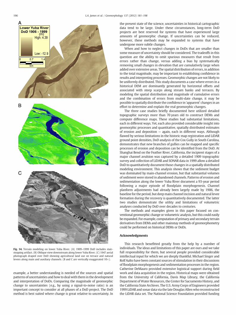
Fig. 14. Terrain modeling on lower Yuba River. (A) 1909–1999 DoD includes stair-stepping artifact. (B) Oblique view downstream along lower Yuba River. (C) 1947 aerialphotograph draped over DoD showing agricultural land use on terrace and naturallevees along main and auxiliary channels. (B and C are vertically exaggerated 10×).
196 L.A. James et al. / Geomorphology 137 (2012) 181–198
example, a better understanding is needed of the sources and spatialpatterns of uncertainties andhow to dealwith them in the developmentand interpretation of DoDs. Comparing the magnitude of geomorphicchange to uncertainties (e.g., by using a signal-to-noise ratio) is animportant concept to consider at all phases of a DoD project. The DoDmethod is best suited where change is great relative to uncertainty. In
the present state of the science, uncertainties in historical cartographicdata tend to be large. Under these circumstances, long-term DoDprojects are best reserved for systems that have experienced largeamounts of geomorphic change. If uncertainties can be reduced,however, these methods may be expanded to systems that haveundergone more subtle changes.
When and how to neglect changes in DoDs that are smaller thansomemeasure of uncertainty should be considered. The tradeoffs in thisquestion are the ability to omit spurious measures that result fromerrors rather than change, versus adding a bias by systematicallyremoving small changes in elevation that are cumulatively large whenadded over extensive areas. The spatial distribution of errors, in additionto the total magnitude, may be important to establishing confidence inresults and interpreting processes. Geomorphic changes are not likely tobe uniformly distributed. This study documents a casewhere errors in ahistorical DEM are dominantly generated by horizontal offsets andassociated with steep scarps along stream banks and terraces. Bymodeling the spatial distribution and magnitude of cumulative errorsand the combination of errors from multi-date change, it may bepossible to spatially distribute the confidence in ‘apparent’ changes in aneffort to determine and explain the real geomorphic changes.
The three case studies briefly documented here utilized detailedtopographic surveys more than 70 years old to construct DEMs andcompute difference maps. These studies had substantial limitations,each in different ways. Yet, each also provided considerable insight intogeomorphic processes and quantitative, spatially distributed estimatesof erosion and deposition — again, each in different ways. Althoughflawed by serious limitations in the historic map registration and LiDARground point densities, DoD analysis of the Cox Gully in South Carolina,demonstrates that new branches of gullies can be mapped and specificprocesses of erosion and deposition can be identified from the DoD. AtShanghai Bend on the Feather River, California, the incipient stages of amajor channel avulsion was captured by a detailed 1909 topographicsurvey and collection of LiDAR and SONAR data in 1999 allow a detailedDoD to quantitatively document those changes in a spatially distributedmodeling environment. This analysis shows that the sediment budgetwas dominated by main-channel erosion, but that substantial volumesof sedimentwere stored in abandoned channels. Patterns of erosion andsedimentation along the lower Yuba River document a 93-year periodfollowing a major episode of floodplain morphogenesis. Channelplanform adjustments had already been largely made by 1906, thebaseline for theperiod, butdeepmain channel incision andnatural leveeformation during the recovery is quantitatively documented. The lattertwo studies demonstrate the utility and limitations of volumetricanalyses conducted by DoD over decades to centuries.
The methods and examples given in this paper focused on con-ventional geomorphic change or volumetric analysis, but this could easilybe expanded. For example, computationof primary and secondary terrainderivatives fromDEMs and othermainstaymethods of geomorphometrycould be performed on historical DEMs or DoDs.
Acknowledgments
This research benefitted greatly from the help by a number ofindividuals. The ideas and limitations of this paper are ours andwe takefull responsibility for them, but several people provided considerableintellectual input for which we are deeply thankful. Michael Singer andRolf Aalto have been constant sources of stimulation in their discussionsoffloodplainmorphogenesis and sedimentation processes in the region.Catherine DeMauro provided extensive logistical support during fieldwork and data acquisition in the region. Historical maps were obtainedfrom the University of California, Davis Map Library, the CaliforniaDepartment ofWater Resources, the Center for SacramentoHistory, andthe California State Archives. TheU.S. ArmyCorps of Engineers provided1999 LiDAR and sonar data via the late Douglas Allenwho reconstructedthe LiDAR data set. The National Science Foundation provided funding

197L.A. James et al. / Geomorphology 137 (2012) 181–198
for a project in this area (BCS 0520933) that helped us to gather the datafrom which much of the case study work was conducted.
References
Aguilar, F.J., Mills, J.P., 2008. Accuracy assessment of LiDAR-derived digital elevationmodels. The Photogrammetric Record 23 (122), 148–169.
Aguilar, F.J., Mills, J.P., Delgado, J., Aguilar, M.A., Negreiros, J.G., Pérez, J.L., 2010.Modelling vertical error in LiDAR-derived digital elevation models. ISPRS Journal ofPhotogrammetry and Remote Sensing 65, 103–110.
Ashmore, P.E., Church, M., 1998. Sediment transport and river morphology: a paradigmfor study. In: Klingeman, P.C., Beschta, R.L., Komar, P.D., Bradley, J.B. (Eds.), Gravel-bed Rivers in the Environment. Water Res. Pubs, CO, pp. 115–148.
Ayres, Associates, 2003. Topographic and hydrographic surveys of the Feather Riversystem for the Sacramento and San Joaquin River Basins Comprehensive Study,California. USACE Contract DACW05-99-D-0010.
Blakemore, M.J., Harley, J.B., 1980. Concepts in the history of cartography: a review andperspective. In: Dahl, E.H. (Ed.), Cartographica 17 (4) (Monograph 26).
Bolstad, P.V., Gessler, P., Lillesand, T.M., 1990. Positional uncertainty in manuallydigitized map data. International Journal of Geographical Information Systems4 (4), 399–412.
Boots, B., Csillag, F., 2006. Categorical maps, comparisons, and confidence. Journal ofGeographical Systems 8, 109–118.
Brasington, J., Langham, J., Rumsby, B., 2003. Methodological sensitivity of morpho-metric estimates of coarse fluvial sediment transport. Geomorphology 53, 299–316.
Butler, D.R., 1989. Geomorphic change or cartographic inaccuracy? A case study usingsequential topographic maps. Surveying and Mapping 49 (2), 67–71.
Butler, D.R., Schipke, K.A., 1992. The strange case of the appearing (and disappearing)lakes: the use of sequential topographic maps of Glacier National Park, Montana.Surveying and Land Information Systems 52 (3), 150–154.
California Debris Commission (CDC), 1906. Map of the Yuba River, California from thenarrows to its mouth in the Feather River. Made under direction of Major Wm. W.Harts, U.S. Army Corps of Engineers, by G. G. McDaniel, Jr., August to Nov., 1906.1:9600; 0.6-m contours.
California Debris Commission (CDC), 1912. Map of Feather River, California fromOroville to southerly limit of gold dredging grounds. Surveyed under direction ofCapt. Thos. H. Jackson, U.S. Army Corps of Engineers by Owen G. Stanley, Sept. -Oct.,1909. 1:9600; 0.6-m contours.
Carrara, A., Bitelli, G., Carla, R., 1997. Comparison of techniques for generating digitalterrain models from contour lines. International Journal of Geographical InformationSciences 11 (5), 451–473.
Carter, J.R., 1988. Digital representation of topographic surfaces. PhotogrammetricEngineering & Remote Sensing 54 (11), 1577–1580.
Cheung, C.K., Shi, W., 2004. Estimation of the positional uncertainty in linesimplification in GIS. The Cartographic Journal 41 (1), 37–45 (9).
Chou, Y.H., 1992. Slope-line detection in a vector-based GIS. PhotogrammetricEngineering and Remote Sensing 58, 227–233.
Chrisman, N.R., 1989. Modeling error in overlaid categorical maps. In: Goodchild, M.,Gopal, S. (Eds.), TheAccuracyof SpatialDatabases. Taylor& Francis, London, pp. 21–34.
Chrisman, N.R., 1999. Speaking truth to power: an agenda for change. In: Lowell, K.,Jaton, A. (Eds.), Spatial Accuracy Assessment: Land Information Uncertainty inNatural Resources. Ann Arbor Press, Chelsea, Michigan, pp. 27–31.
Cobby,D.M.,Mason, D.C., Davenport, I.J., 2001. Image processing of airborne scanning laseraltimetry data for improved river flood modeling. ISPRS Journal of Photogrammetryand Remote Sensing 56, 121–138.
Defourny, P., Hecquet, G., Philippart, T., 1999. Digital terrain modeling: accuracyassessment and hydrological simulation sensitivity. In: Lowell, K., Jaton, A. (Eds.),Spatial Accuracy Assessment: Land Information Uncertainty in Natural Resources.Ann Arbor Press, Chelsea, Michigan, pp. 61–70.
Duan, J., Grant, G.E., 2000. Shallow landslide delineation for steep forest watersheds basedon topographic attributes and probability analysis. In: Wilson, J.P., Gallant, J.C. (Eds.),Terrain Analysis: Principles and Applications. J. Wiley & Sons, N.Y, pp. 311–329.
Federal Geographic Data Committee (FGDC), 1998. Geospatial Positioning AccuracyStandards. FGDC-STD-007-1998. http://www.fgdc.gov/standards/ (accessed May,2010).
Ferguson, R.I., Ashworth, P.J., 1992. Spatial patterns of bedload transport and channelchange in braided and near-braided rivers. In: Billi, P., Hey, R.D., Thorne, C.R.,Tacconi, P. (Eds.), Dynamics of Gravel Bed Rivers. J. Wiley, pp. 477–495.
Fisher, P.F., Tate, N.J., 2006. Causes and consequences of error in digital elevationmodels. Progress in Physical Geography 30, 467–489.
Fonstad, M.A., Marcus,W.A., 2005. Remote sensing of stream depths with hydraulically-assisted bathymetry (HAB) models. Geomorphology 72 (4), 320–339.
Gaeuman, D.A., Schmidt, J.C., Wilcock, P.R., 2003. Evaluation of in-channel gravelstorage with morphology-based gravel budgets developed from planimetric data.Journal of Geophysical Research 108 (F1), 6001.
García-Quijano, M.J., Jensen, J.R., Hodgson, M.E., Hadley, B.C., Gladden, J.B., Lapine, L.A.,2008. Significanceof altitude andpostingdensityonLiDAR-derivedelevation accuracyon hazardous waste sites. Photogrammetric Engineering & Remote Sensing 74 (9),1137–1146.
Ghoshal, S., James, L.A., Singer, M., Aalto, R., 2010. Channel and floodplain change analysisover a 100-year period: Lower Yuba River, California. Remote Sensing 2, 1797–1825.doi:10.3390/rs2071797. Open Access: www.mdpi.com/journal/remotesensing.
Gomez, B., 1991. Bedload transport. Earth Science Reviews 31 (2), 89–132.Gottsegen, J., Montell, D., Goodchild, M., 1999. A comprehensivemodel of uncertainty in
spatial data. In: Lowell, K., Jaton, A. (Eds.), Spatial Accuracy Assessment: Land
Information Uncertainty in Natural Resources. Ann Arbor Press, Chelsea, Michigan,pp. 175–181.
Griffith, D.A., Haining, R.P., Arbia, G., 1999. Uncertainty and error propagation in mapanalyses involving arithmetic and overlay operations: inventory and prospects. In:Lowell, K., Jaton, A. (Eds.), Spatial Accuracy Assessment: Land InformationUncertainty in Natural Resources. Ann Arbor Press, Chelsea, Michigan, pp. 11–25.
Guptill, S.C., Morrison, J.L. (Eds.), 1995. Elements of Spatial Data Quality. Internat.Cartographic Assn., Oxford. Elsevier, New York (202pp.).
Guth, P.L., 1999. Contour line “Ghosts” in USGS Level 2 DEMs. PhotogrammetricEngineering & Remote Sensing 65 (3), 289–296.
Harley, J.B., 1968. The evaluation of early maps: towards a methodology. Imago Mundi22, 62–74.
Henderson, T., 1984. A Study of the Precision and Absolute Horizontal Accuracy of USGSDigital Line Graph Point Data, Draft (US Geological Survey).
Heritage, G.L., Milan, D.J., Large, A.R.G., Fuller, I.C., 2009. Influence of survey strategy andinterpolation model on DEM quality. Geomorphology 112, 334–344.
Hodgson, M.E., Alexander, B.E., 1990. Use of historic maps in GIS analyses, ACSM Tech.Papers, 1990 ASPRS-ACSM Annual Convention, 3, pp. 109–116.
Hodgson, M.E., Bresnahan, P., 2004. Accuracy of airborne LiDAR-derived elevation:empirical assessment and error budget. Photogrammetric Engineering & RemoteSensing 70 (3), 331–339.
Hodgson, M.E., Jensen, J.R., Schmidt, L., Schill, S., Davis, B., 2003. An evaluation of LiDARand IFSAR-derived digital elevation models in leaf-on conditions with USGS Level 1and Level 2 DEMs. Remote Sensing of Environment 84 (2), 295–308.
Hodgson, M.E., Jensen, J.R., Raber, G., Tullis, J., Davis, B., Schuckman, K., Thompson, G.,2005. An evaluation of LiDAR-derived elevation and terrain slope in leaf-offconditions. Photogrammetric Engineering and Remote Sensing 71 (1), 817–823.
Hooke, J., Perry, R.A., 1976. The planimetric accuracy of tithe maps. Cartographic Journal13, 177–183.
Hu, B., 2001. Assessing the accuracy of the map of the Prefectural Capital of 1261 usinggeographic information systems. The Professional Geographer 53 (1), 32–44.
Hughes, M.L., McDowell, P.F., Marcus, W.A., 2006. Accuracy assessment of georectifiedaerial photos: implications for measuring lateral channel movement in a GIS.Geomorphology 74, 1–16.
Hutchinson, M.F., Gallant, J.C., 2000. Digital elevation models and representation ofterrain shape. In: Wilson, J.P., Gallant, J.C. (Eds.), Terrain Analysis: Principles andApplications. N.Y, J. Wiley, pp. 29–50.
International Cartographic Association (ICA), 1973. Multilingual Dictionary ofTechnical Term in Cartography. ICA, Commission II. Franz Steiner Verlag,Wieshaden. (573 pp.).
Ireland, H.A., Sharpe, C.F.S., Eargle, D.H., 1939. Principles of Gully Erosion in thePiedmont of South Carolina. U.S. Dept. Agriculture Tech, p. 633.
James, L.A., Watson, D.G., Hansen, W.F., 2007. Using LiDAR to map gullies andheadwater streams under forest canopy: South Carolina, USA. Catena 71, 132–144.
James, L.A., Singer, M.B., Ghoshal, S., Megison, M., 2009. Sedimentation in the lowerYuba and Feather Rivers, California: long-term effects of contrasting river-management strategies. In: James, L.A., Rathburn, S.L., Whittecar, G.R. (Eds.),Management and Restoration of Fluvial Systems with Broad Historical Changes andHuman Impacts: Geol. Soc. Amer. Spec. Paper, 451.
Jenks, G.F., 1981. Lines, computers, and human frailties. Annals Assn. Amer.Geographers 71 (1), 1–10.
Jensen, J.R., 2007. Remote sensing of the environment: an Earth resource perspective,2nd Ed. Prentice Hall, Upper Saddle River, NJ.
Keefer, B.J., Smith, J.L., Gregoire, T.G., 1991. Modeling and evaluating the effects ofstreammode digitizing errors on map variables. Photogrammetric Engineering andRemote Sensing 57 (7), 957–963.
Kolomechuk, C., 2001. Gully Erosion in Spartanburg County from 1939 to 2001. Unpub.M.S. thesis, Geography Dept., Univ. South Carolina.
Lane, S.N., 2000. The measurement of river channel morphology using digitalphotogrammetry. Photogrammetric Record 16 (96), 937–961.
Lane, S.N., Chandler, J.H., Richards, K.S., 1994. Developments in monitoring andmodelling small scale riverbed topography. Earth Surface Processes and Landforms19, 349–368.
Lane, S.N., Richards, K.S., Chandler, J.H., 1995. Morphological estimation of the time-integrated bedload transport rate. Water Resources Research 31, 761–772.
Lane, S.N., Westaway, R.M., Hicks, D.M., 2003. Estimation of erosion and depositionvolumes in a large, gravel-bed braided river using synoptic remote sensing. EarthSurface Processes and Landforms 28, 249–271.
Langran, G., 1992. Time in Geographic Information Systems. Taylor and Francis, London.Laxton, P.P., 1976. The geodetic and topographical evaluation of English county maps,
1740–1840. The Cartographic Journal 13, 37–54.Li, Z., 1991. Effects of check points on the reliability of DTM accuracy estimates obtained
from experimental tests. Photogrammetric Engineering and Remote Sensing 57 (10),1333–1340.
Lindsay, J.M., 1980. The assessment of transient patterns on historic maps — a casestudy. The Cartographic Journal 17, 16–20.
Livieratos, E., 2006. On the study of the geometric properties of historical cartographicrepresentations. Cartographica 41 (2), 165–175.
Lloyd, R., Gilmartin, P., 1987. The South Carolina coastline on historical maps: acartometric analysis. The Cartographic Journal 24, 19–26.
Maling, D.H., 1989. Measurements from maps: principles and methods of cartometry.Pergamon Press, N.Y. 577 pp.
Marcus, W.A., Fonstad, M.A., 2008. Optical remote mapping of rivers at sub-meterresolutions and watershed extents. Earth Surface Processes and Landforms 33, 4–24.
Mark, D.M., 1984. Automated detection of drainage networks from digital elevationmodels. Cartographica 21, 168–178.

198 L.A. James et al. / Geomorphology 137 (2012) 181–198
Marsden, L.E., 1960. How the national map accuracy standards were developed. Surv.Mapp. 20, 427–439.
Martin, Y., Ham, D., 2005. Testing bedload transport formulae using morphologictransport estimates and field data: lower Fraser River, British Columbia. EarthSurface Processes and Landforms 30, 1265–1282.
Martínez-Casasnovas, J.A., Ramos, M.C., Poesen, J., 2004. Assessment of sidewall erosion inlarge gullies using multi-temporal DEMs and logistic regression analysis. Geomor-phology 58, 305–321.
Megison,M., 2008. Quantifying channel changeswith historical maps and high-resolutiontopographic data: Lower Feather River, California, 1909–1999. Unpub. Master thesis,Geog. Dept., Univ. South Carolina; 142 pp.
Mendell, Col.G.H., 1881. Protection of the navigable waters of California from injuryfrom the debris of mines. U.S. Congress, House Document 76, 46th Congress, 3rdSession.
Morrison, J.L., 1995. Spatial data quality. In: Guptill, S.C., Morrison, J.L. (Eds.), Elements ofSpatial Data Quality. Elsevier for International Cartographic Soc, Oxford, pp. 1–12.
Mowrer, H.T., 1999. Accuracy (re)assurance: selling uncertainty to the uncertain. In:Lowell, K., Jaton, A. (Eds.), Spatial Accuracy Assessment: Land InformationUncertainty in Natural Resources. Ann Arbor Press, Chelsea, Michigan, pp. 3–10.
National Institute of Standards and Technology (NIST), 1994. Federal Information ProcessingStandard Publication173. (Spatial Data Transfer Standard, Part 1, Version 1.1). U.S. Dept.of Commerce, Wash., D.C.
Nelson, A., Reuter, H.I., Gessler, P., 2009. DEM production methods and sources. In:Hengl, T., Reuter, H. (Eds.), Geomorphometry, Concepts, Software, Applications.Developments in Soil Science, Vol. 33. Elsevier, Oxford.
O'Sullivan, D., 2005. Geographical information science: time changes everything.Progress in Human Geography 29 (6), 749–756.
Pelletier, J.D., 2008. Quantitative modeling of Earth surface processes. Cambridge Univ.Press, Cambridge. 295 pp.
Peuquet, D.J., 2003. Representations of space and time. Guilford Press, New York.Pike, R., 1995. Geomorphometry – progress, practice and prospect. Zeitschrift für
Geomorphologie, N.F. Supplement Band 101, 221–238.Pike, R.J., Evans, I.S., Hengl, T., 2009.Geomorphometry:a brief guide. In:Hengl, T., Reuter, H.
(Eds.), Geomorphometry, Concepts, Software, Applications. Developments in SoilScience, Vol. 33. Elsevier, Oxford.
Raber, G.T., Jensen, J.R., Hodgson, M.E., Tullis, J.A., Davis, B.A., Berglund, J., 2007. Impactof LiDAR nominal post-spacing on DEM accuracy and flood zone delineation.Photogrammetric Engineering and Remote Sensing 73 (7), 793–804.
Raper, J., 2000. Multidimensional geographic information science. Taylor and Francis,London.
Ravenhill, W., Gilg, A., 1974. The accuracy of early maps? Towards a computer aidedmethod. The Cartographic Journal 11 (1), 48–52.
Rumsby, B.T., Brasington, J., Langham, J.A., McLelland, S.J., Middeton, R., Rollinson, G.,2008. Monitoring and modelling particle and reach-scale morphological change ingravel-bed rivers: applications and challenges. Geomorphology 93, 40–54.
Schumm, S.A., 1991. To interpret the Earth: ten ways to bewrong. Cambridge Univ. Press,N.Y. 131 pp.
Stoker, J., Harding, D., Parrish, J., 2008. The need for a national LiDAR dataset.Photogrammetric Engineering & Remote Sensing 74 (9), 1066–1068.
Stone, J.C., Gemmell, A.M.D., 1977. An experiment in the comparative analysis ofdistortion on historical maps. The Cartographic Journal 14, 7–11.
Stonestreet, S.E., Lee, A.S., 2000. Use of LIDAR Mapping for Floodplain Studies, paperpresented at Building Partnerships-2000 Joint Conference on Water ResourceEngineering, Planning, and Management.
Tobler, W.R., 1966. Medieval distortions: the projections of ancient maps. Annals, Assn.Amer. Geographers 56, 351–360.
Towill, Inc., 2006. Project Report for topographic surveys of the Lower Feather and BearRivers for the Sacramento and San Joaquin River Basins Comprehensive Study,California. Contract No.: DACW05-99-D-0005 for U. S. Army Corps of Engineers,Sacramento District.
Townsend, P.A., Walsh, S.J., 1998. Modeling floodplain inundation using an integratedGIS with radar and optical remote sensing. Geomorphology 21, 295–312.
Traylor, C.T., 1979. The evaluation of a methodology to measure manual digitizing errorin cartographic data bases. Unpub. Ph.D. Diss. (Dept. Geography and Meteorology:Univ. Kansas).
U.S. Geological Survey (USGS), 1999. Map accuracy standards fact sheet FS-171–99.http://egsc.usgs.gov/isb/pubs/factsheets/fs17199.html#US%20National (AccessedMay, 2010).
Veregin, H., 1989. Error modeling for themap overlay operation. In: Goodchild, M., Gopal,S. (Eds.), The Accuracy of Spatial Databases. Taylor & Francis, London, pp. 3–18.
Von Schmidt, A.M., 1859. Plat of the New Helvetia Rancho finally confirmed to John A.Sutter. Surveyed by A. M. Von Schmidt, Deputy Surveyor, Sept.–Oct., 1859. Scale1:63,360 (80 chains to an inch), 1 sheet. Center for Sacramento History, SacramentoCounty Recorder's Office Collection.
Walker, J.P., Willgoose, G.R., 1999. On the effect of digital elevation model accuracy onhydrology and geomorphology. Water Resources Research 35, 2259–2268.
Walsh, S.J., 1989. User considerations in landscape characterization. In: Goodchild, M.,Gopal, S. (Eds.), TheAccuracyof Spatial Databases. Taylor&Francis, London, pp. 35–43.
Walsh, S.J., Lightfoot, D.R., Butler, D.R., 1987. Recognition and assessment of error ingeographic information systems. Photogrammetric Engineering and Remote Sensing53 (10), 1423–1430.
Wescoatt, N., 1861. Official Map of Yuba County California compiled and drawn fromofficial surveys by N. Wescoatt 1861. Map collection, Shields Library, U. C. Davis.
Wheaton, J.M., Brasington, J., Darby, S.E., Sear, D., 2009. Accounting for uncertainty inDEMs from repeat topographic surveys: improved sediment budgets. Earth SurfaceProcesses and Landforms 35 (2), 136–156.
White, R., 2006. Pattern based map comparisons. Journal of Geographic Systems 8,145–164.
Wikle, C.K., Cressie, N., 2000. Space-time statistical modeling of environmental data. In:Mowrer, H.T., Congalton, R.G. (Eds.), Quantifying Spatial Uncertainty in NaturalResources: Theory and Applications for GIS and Remote Sensing. Ann Arbor Press,Chelsea, Michigan, pp. 213–235.
Wood, J.D., Fisher, P.F., 1993. Assessing interpolation accuracy in elevation models. IEEEComputer Graphics & Applications 48–56.