Geometric Verification of Swirling Features in Flow Fields

Ming Jiang ∗

The Ohio State UniversityRaghu Machiraju ∗

The Ohio State UniversityDavid Thompson †

Mississippi State University

Figure 1: Geometric verification algorithm applied to the test tornado dataset from LLNL [3].

ABSTRACT

In this paper, we present a verification algorithm for swirling fea-tures in flow fields, based on the geometry of streamlines. The fea-tures of interest in this case are vortices. Without a formal defi-nition, existing detection algorithms lack the ability to accuratelyidentify these features, and the current method for verifying theaccuracy of their results is by human visual inspection. Our ver-ification algorithm addresses this issue by automating the visual in-spection process. It is based on identifying the swirling streamlinesthat surround the candidate vortex cores. We apply our algorithmto both numerically simulated and procedurally generated datasetsto illustrate the efficacy of our approach.

Keywords: feature verification, vortex detection, flow field visu-alization

1 INTRODUCTION

Large-scale computational fluid dynamics simulations of physicalphenomena produce data of unprecedented size. Unfortunately, de-velopment of appropriate data management and visualization tech-niques has not kept pace with the growth in size and complex-ity of such datasets. One paradigm for large-scale visualizationis to browse regions containing significant features of the datasetwhile accessing only the data needed to reconstruct these regions.The cornerstone of this visualization paradigm is a representational

∗jiang, raghu@cis.ohio-state.edu†dst@erc.msstate.edu

scheme that facilitates progressive access to macroscopic featuresin the dataset [10]. In this approach, an automatic feature detec-tion algorithm is used to accurately identify and rank contextuallysignificant features.

In general, a feature can be defined as a pattern occurring in adataset that is the manifestation of correlations among various com-ponents of the dataset. The swirling features in flow fields, whichare the central subject of this paper, are commonly called vortices.By most accounts [9, 12, 13], a vortex is characterized by swirlingmotion of fluid around a central region. From the morning coffee tothe evening bath, it is perhaps one of the most common and naturalphenomena occurring in everyday life. Yet, it’s very definition stilleludes those who are active in its pursuit.

Despite this lack of formalism, various detection algorithms ex-ist that can identify, to a certain degree, these swirling features. Themain deficiency common to these algorithms is not the false posi-tives which they may produce, but rather their inability to distin-guish the false positives from the true swirling features. For many,this is due to their heavy reliance on the velocity gradient tensoras a local tool for identifying global features, such as vortices [4].As noted by Thompson et al. [19], these local techniques are in-herently problematic because they do not incorporate the necessaryinformation into their detection process for a global feature.

The ability to verify the correctness of a candidate feature is es-sential for any feature-based visualization paradigm. Feature verifi-cation can not only improve the quality of the identification process,but also improve its overall performance by obviating the need toapply computationally expensive detection algorithms at all pointsin the field. Inexpensive and less accurate techniques can be usedto identify candidate features which are then subjected to the ver-ification process. By operating only on the candidate features, themore expensive verification process is made computationally effi-cient. This modus operandi is indispensible in the context of large-scale datasets. Further, for features such as vortices, aggregate ver-

ification techniques can be developed that capture the global natureof the feature [19].

In this paper, we present an automatic verification algorithm for3D swirling features in flow fields. This work is an extension fromour previous work [7] on efficiently detecting vortex core regions.We present a geometric approach to verifying vortices that is mostconsistent with the notion of a swirling flow. In the absence of aformal definition, this is the most logical approach to take for sucha visually recognizable feature. Given a candidate vortex core, wemeasure certain differential geometry properties of the surround-ing streamlines to determine whether or not these streamlines areswirling around the core region. If the streamlines satisfy our 2πswirling criterion for 3D vortices, then from a geometric perspec-tive, the candidate vortex core is an actual vortex core.

Our paper is structured as follows. We first provide a brief reviewof existing vortex detection algorithms and discuss some of the is-sues involved in vortex definition. We then describe the vortex coreregion detection algorithm that we use to identify candidate vortexcores. Then, we provide the implementation details behind our ver-ification algorithm and the results that demonstrate the efficacy ofour approach. Finally, we draw conclusions as to the relative meritsof our feature verification algorithm.

2 PREVIOUS WORK

To our knowledge, no attempts have been made to address the issueof feature verification as a post-processing step of feature detectionin computational datasets. Although Peikert and Roth [11, 14] havesuggested using their parallel vectors operator to corroborate theresults from another detection operator, their suggested approachlacks the ability to exploit the initial detected results for computa-tional efficiency. More importantly, their suggested approach offerslittle to address the issue of dealing with false positives.

For completeness, we briefly review several detection algorithmsin the literature. Though these reviews are not meant to be exhaus-tive, they provide a fairly good overview of the state of the art indetecting vortices in flow fields. The detection algorithm chosen forverification is based on our previous work [7] on efficiently detect-ing vortex core regions. We defer its discussion to a later section. Itshould be noted that each of these algorithms described below maygenerate false positives and miss otherwise obvious vortices.

The first group of methods is based on isosurfaces of a scalarfield. Levy et al. [8] developed a method on the assumption thata vortex core is located in a region where the normalized helicityV·(∇V)|V||∇V| approaches ±1. In Berdahl and Thompson’s [2] method,the assumption is that two of the eigenvalues of the velocity gradi-ent tensor are a complex conjugate pair in regions of swirling flow.A parameter termed the “swirl” is defined at each point in the do-main using the magnitude of the imaginary part of the conjugatepair and the velocity in the plane perpendicular to the eigenvector.According to [2], the swirl is nonzero in regions containing vorticesand attains a local maximum in the core region.

Jeong and Hussian [6] defined a vortex based on the symmetricdeformation tensor S and the antisymmetric spin tensor Ω. Accord-ing to [6], if the second largest eigenvalue of S2 + Ω2 is negative ata point, that point is contained within a vortex. Additionally, if thesecond invariant of the velocity gradient tensor 1

2

(|Ω|2−|S|2

)is

positive at a point, the point is contained within a vortex. The maindisadvantage with these methods is their difficulty in automaticallydistinguishing the individual vortices.

The second group of methods is based on the extraction of vor-tex core lines. Banks and Singer [1] developed a predictor-correctoralgorithm based on the assumptions that the vortex core is a vortic-ity line (a streamline in the vorticity field) and that pressure shouldbe minimum in the core. Sujudi and Haimes [18] described a line-

based method that extracts the vortex core by locating points thatsatisfy the following two conditions: 1) the velocity gradient tensorhas a pair of complex eigenvalues and 2) the velocity in the planeperpendicular to the real eigenvector is zero. By connecting thesepoints, a line segment representing the vortex core is constructed,though it is not always possible to form a contiguous line. To ad-dress this problem, Haimes and Kenwright [4] recast the algorithmto be face-based rather than cell-based.

Roth and Peikert [15] proposed a different approach for detectingcore lines using the parallel vector operator. Rather than perform-ing an eigen-analysis on the velocity gradient tensor, their algorithmdetects for parallel alignment between the velocity vector and theacceleration vector. Their approach was especially designed for tur-bomachinery datasets, which often contain weakly rotating vorticeswith nonnegligible curvature. Whereas Sujudi and Haimes’ [18]method has difficulty with curved vortices, theirs’ performs a cor-rection for the curvature by taking second-order derivatives into ac-count. The main disadvantages with these methods are their com-putational complexity and inability to produce contiguous lines.

The third group of methods is based on the geometric propertiesof streamlines. Portela [12] developed a collection of mathemati-cally rigorous definitions for a vortex, using set theory and differen-tial geometry. Essentially, his definitions are based on the idea that avortex is comprised of a central core region surrounded by swirlingstreamlines. His 2D method detects vortices by verifying whetheror not the winding angle of streamlines around a grid point is ascalar multiple of 2π . Sadarjoen et al. [16, 17] proposed a simpli-fication to the 2D winding-angle method, by using the summationof signed angles along a streamline instead. The main disadvantagewith these methods is that they lack a viable 3D counterpart to their2D approach – winding angles are only meaningful in 2D.

3 SWIRLING FEATURES

Without a formal definition, it is not unreasonable to consider a vor-tex as a swirling feature. Among the existing definitions, the asso-ciation of swirling motion with the presence of a vortex is the mostcommon thread. This association stems from our visual perceptionof the swirling phenomena that are pervasive throughout the natu-ral world. However, translating that perceptual understanding of avortex into a formal definition has been quite a challenge. The dif-ficulty lies in the generality of such definitions. Lugt [9] proposedthe following definition for the presence of a vortex.

A vortex is the rotating motion of a multitude of materialparticles around a common center.

The problem with this definition is that it is too vague. Althoughit is consistent with visual observations, it does not lend itself read-ily to designs for a detection algorithm. Terms such as rotating mo-tion and material particles are easy to conceptualize, but difficult toimplement. In light of this, Robinson [13] attempted to provide amore concrete definition of a vortex, by specifying the conditionsfor detecting rotating motion in 3D.

A vortex exists when instantaneous streamlines mappedonto a plane normal to the vortex core exhibit a roughlycircular or spiral pattern, when viewed from a referenceframe moving with the center of the vortex core.

The primary shortcoming of this definition is that it is self-referential: the existence of a vortex requires knowing the direc-tion of its core. Additionally, no one has been able to utilize it forthe development of an effective detection algorithm [1]. In general,it is difficult to detect the correct reference frames for all types ofvortical flows.

More recently, Portela [12] developed a collection of mathemat-ically rigorous definitions for a vortex, using elementary tools fromset theory and differential geometry. Although his 2D definitionsare replete with pedantries and subtleties, his 3D definitions ap-pear less novel and ultimately resemble those of Robinson’s [13].However, the intuition behind his definitions is quite simple andgeneral: a vortex is comprised of a central core region surroundedby swirling streamlines. He appealed to the Jordan Curve Theoremto distinguish the central core region of a vortex and the windingangle concept to measure the swirling of streamlines. The windingangle of a streamline measures the rotation of that streamline withrespect to a given point. Satisfying the swirling criterion meansthe streamline must have a winding angle of at least 2π . Note thatthis approach is inherently limited to 2D. Whereas in 2D, curvaturealone dictates the rotation of a planar curve, in 3D, both curvatureand torison dictate the bending and twisting of the space curve.

4 DETECTION ALGORITHM

As a pre-processing step to the verification algorithm, most of theexisting detection algorithms would suffice. The only requirementis that the output of the detection algorithm must be vortex cores,in the form of either lines or regions. In the case of vortex corelines, the collection of grid cells intersected by the core line is usedas input to the verification algorithm. The necessity of this con-version will become clear in the next section when we discuss theverification algorithm in detail.

The detection algorithm we chose in this case is from our pre-vious work [7] on efficiently detecting vortex core regions. In thisapproach, a combinatorial labeling scheme is employed to identifyall the grid points that belong to vortex cores and aggregate theminto individual regions. Unlike most of the existing detection meth-ods, this labeling scheme is extremely efficient, and its efficacy hasbeen demonstrated in [7]. What makes this approach so effective atdetecting vortex core regions is its close resemblence to Sperner’slemma from Fixed Point Theory in combinatorial topology.

Swirl Plane

i i+1i−1

j−1

j+1

k−1

k+1

k

j

A

CB

E

Figure 2: 3D vortex core region detection algorithm.

The connection between vortices and fixed points (i.e. criticalpoints) are well known [18]. Whereas the Sperner’s lemma labelsthe vertices of a simplex and identifies the fixed points of a labeledsubdivision [5], the detection algorithm labels the velocity vectorsof the grid points and identifies grid cells that are most likely to

contain critical points. Each velocity vector is labeled according tothe direction in which it points. Since velocity vectors around coreregions exhibit certain flow patterns that are unique to vortices, itis sufficient to examine the immediate neighborhood of a grid pointfor the existence of those flow patterns. This procedure is sufficientfor detecting 2D vortex core regions.

In 3D, it is necessary to approximate the core direction vectorfirst, and then project the neighboring velocity vectors onto theplane normal to it, before applying the above procedure to the pro-jected velocity vectors. We refer to this plane as the swirl planebecause instantaneous streamlines projected onto this plane exhibita swirling pattern that is commonly associated with 2D vortices.Figure 2 illustrates the 3D algorithm, along with the swirl planeand the combinatorial labeling scheme. Potential candidates forthe core direction vector include the vorticity vector [1], which isone of the least computationally intensive methods, and the realeigenvector [18], which is one of the most computationally inten-sive methods. What makes the 3D algorithm unique is its relativeinsensitivity to core direction approximations. In the detection pro-cess, using the vorticity vector to approximate the core directionvector can be just as effective as using the real eigenvector.

The advantage of this approach over other vortex core regiondetection algorithms is its ability to segment the core regions in-dividually. This would allow the verification algorithm to proceeddirectly without any extra processing. Its advantage over vortexcore line detection algorithms is its computational efficiency, dueto the combinatorial nature of the detection algorithm. Althougha vortex core line can more precisely represent a vortex core, thisdoes not imply its detection process is more accurate. This increasein the precision of representation can effect an increase in the com-plexity of the detection process, a tradeoff that is unnecessary in thecontext of the verification algorithm.

5 GEOMETRIC VERIFICATION

With the existing detection algorithms, one of the most effectivemeans to ascertain the accuracy of the detected results is throughvisual inspection. By seeding streamlines near the detected vortexcores, one can visualize the swirling patterns that are generally as-sociated with vortices. Both [15] and [18] utilized this strategy tobuild a convincing argument for the validity of their results. Theproblem with visual inspection is that it requires human interven-tion, a process that is contrary to the automatic nature of the de-tection algorithm. And in the context of large-scale datasets, theinspection process becomes highly infeasible.

The geometric verification algorithm we propose addresses theabove issue by automating the visual inspection process. Since for-mal verification is not possible without a formal definition, geomet-ric verification is the logical alternative. By identifying the swirlingpatterns surrounding a candidate vortex core, our verification algo-rithm can arbitrate the presence or absence of a vortex most con-sistently with visual scrutiny. Although there are limitations to thevisual inspection process, it is more practical to formalize that pro-cess, as a way to address the false positive issue, than to proposeyet another vortex definition.

Given a candidate vortex core, the underlying goal of our geo-metric verification algorithm is to identify the swirling streamlinessurrounding it, by using elementary differential geometry proper-ties of the streamlines. For the 2D case, both [12] and [17] havepresented methods that are sufficent for identifying planar swirlingstreamlines. As described previously, these methods involve mea-suring the winding angle of a planar streamline and checking ifthe winding angle is at least 2π , which is a clear indication thatthe streamline is swirling. However, both approaches cannot be di-rectly extended into 3D, because the winding angle measurementthey use is inherently 2D.

To remedy this problem, Portela [12] proposed reducing theproblem from 3D to 2D by projecting the local velocity vectors ontothe plane normal to the vortex core direction, the swirl plane. Notethat this is similiar to what Robinson [13] proposed as the definitionof a vortex. The problem with this approach is deciding which lo-cal velocity vectors to project onto the swirl plane. Not only wouldthere be an issue with the size of the projected neighborhood, sothat enough velocity vectors are projected onto the swirl plane toapply the 2D algorithm, but also with the distortion caused by theprojected grid structure. To our knowledge, no viable algorithmbased on Portela’s [12] proposed idea exists.

Similarly, projecting streamlines onto a swirl plane, as Robin-son [13] has proposed, is also problematic because the core direc-tion along a vortex core can vary depending on the curvature ofthe vortex core. Like tangents along a space curve, the directionvector at a particular point along a vortex core only approximatesthe core direction within a small neighborhood. Therefore, as soonas the streamline is traced outside of that neighborhood, the valid-ity of the projected streamline on the swirl plane becomes suspect.The situation is exacerbated by slowly rotating streamlines aroundcurved vortex cores, such as those in turbomachinary flow fields de-scribed by [15]. As Banks and Singer [1] correctly pointed out, thisapproach does not lend itself conveniently to a viable algorithm.

Measuring the swirling of a 3D streamline is a nontrivial prob-lem. The difficulty arises from streamlines that swirl around curvedvortex cores. As the deficiency in Robinson’s [13] proposal illus-trates, the measurement process for 3D swirling has to take intoaccount the curvature of the vortex core. To address this issue, weintroduce probe vectors, which can be computed along a stream-line at each point. As its name suggests, a probe vector probes thevortex core for the direction vector at that particular point. Since adirection vector approximates the local behavior of a vortex core,it provides the necessary curvature information to the measurementprocess.

We also introduce a local alignment process, based on the probeddirection vectors, to accommodate vortex cores with nontrivial cur-vatures. The process individually rotates the direction vectors toalign with the z-axis, and then applies the same transformation tothe streamline. From a streamline’s perspective, this transformationwould locally straighten any curved vortex cores. Consequently,the transformed streamline can be projected onto the (x,y)-planefor the 2D winding angle computation. However, locally trans-forming the streamline can result in irregular geometry, because thealignment transformation is nonuniform for curved vortex cores. Toavoid this problem, we transform the tangent vectors of a stream-line instead. In tangent space, the transformed tangent vectors areprojected onto the (x,y)-plane to create a tangent profile. Ratherthan computing the winding angle of the projected streamline, wecompute the angle spanned by the tangent profile to determine if itsatisfies the 2π swirling criterion.

Before discussing the implementation details of our geometricverification algorithm, we illustrate it using two canonical exam-ples from the literature: the Rankine vortex and the bent helicalvortex. These two vortices are ideal for demonstrating the geomet-ric verification process, because the geometry of their streamlinesare uniform.

5.1 Rankine VortexA fluid motion composed of a solid body rotation with angular ve-locity Ω within a certain radius R and a potential vortex outside ofthis radius is called a Rankine vortex [9]. The Rankine vortex is agood model for a real vortex because of the concentrated vorticityin its core region and the decay of the circumferential velocity asthe distance from the core is increased. For the three-dimensionalvortex, we have added a constant velocity U along the axis of the

Figure 3: 3D Rankine vortex

vortex (in this case, the z-axis). The equations describing the veloc-ity field of the Rankine vortex are given in cylindrical coordinates(r,θ ,z) by

ur = 0

uθ =

Ω r, r ≤ R

Ω R2

r , r > R

uz = U

(1)

The velocity field defined by Equation 1 satisfies the continuityequation for incompressible flow and therefore represents a kine-matically possible velocity field. Figure 3 illustrates a Rankine vor-tex with R = 0.1 and Ω = 10. The velocity field was generatedon a 1283 cartesian grid. The yellow region is an extracted isosur-face, representing the vortex core region, and the blue lines are theswirling streamlines, seeded near the vortex core region.

(a) (b)

(c)

Figure 4: A streamline seeded near a Rankine vortex: (a) Tangentvectors, (b) probe vectors and (c) tangent profile.

Figure 4 illustrates the tangent vectors, probe vectors and tangentspace computed along a streamline. The dark green arrows alongthe streamline in Figure 4(a) are the tangent vectors. The orangered arrows pointing toward the vortex core in Figure 4(b) are the

Figure 5: Steady progression of the verification process for theRankine vortex: (left) one-third and (right) two-third of a completespiral.

probe vectors. And Figure 4(c) is the tangent space, in which thetangent vectors are projected onto the (x,y)-plane to generate thetangent profile.

To illustrate the geometric verification process, we seeded astreamline near the vortex core and traced it for one-third of a spiral,and then for another one-third. This is illustrated in Figure 5. Fig-ure 5(left) illustrates the first third and Figure 5(right), the secondthird. Note the steady progression of the tangent profile around the(x,y)-plane as the streamline spirals around the vortex core. Eachcomplete spiral corresponds to a complete revolution in the (x,y)-plane of the tangent space.

5.2 Bent Helical VortexThe bent helical vortex is an important model for turbomachineryflow fields [14]. The model consists of a helical flow field built froma rigid rotation in the (x,z)-plane, a constant motion in y-directionand a bent of radius R in the (x,y)-plane. The velocity field for thebent helical vortex is given in the (x,y,z) coordinate system by

ux = −ω x z Rr2 − γ y

r

uy = −ω y z Rr2 +

γ xr

uz =

(R − R2

r

)ω

(2)

where r =√

x2 + y2.

R is the radius to which the vortex core is bent, γ is the axialcomponent along the core, and ω is the rotation component aboutthe core. This flow field has zero divergence (i.e. it conserves massfor a incompressible medium), but it is not an exact solution ofthe Navier-Stokes equations, and it possesses a singularity on thez-axis. However, in the vortex core region there are no singulari-ties or critical points, and similar flow patterns have been found innumerical solutions from a Navier-Stokes solver [14].

Figure 6: Bent helical vortex [14]

Figure 6 illustrates a bent helical vortex with R = 1, ω = 6 andγ = 0.5. The velocity field was generated on a 1283 cartesian grid.The yellow region represents the detected vortex core, and the bluelines, the swirling streamlines. Clearly, the vortex core is curvedwith a nontrivial curvature. To illustrate the efficacy of our localalignment transformation, we seed a streamline near one end ofthe bent vortex core and compute its tangent space both with andwithout the transformation. Figure 7(left) illustrates the streamline,along with its tangent vectors and probe vectors. Figure 7(right)illustrates both tangent spaces. The difference between the two isquite clear: without transformation, the tangent vectors can pointin various directions without any particular order, and with trans-formation, the tangent vectors uniformly revolve around the z-axis,forming a cone shape with its apex at the origin of the tangent space.

Figure 7: Difference between tangent profiles with (bottom) andwithout (top) the local alignment transformation.

To demonstrate the effectiveness of our geometric verificationalgorithm on slowly rotating, curved vortices, we conducted severalexperiments using the bent helical vortex model, with R = 1, γ =0.5, and ω varying from 6 down to 1. Figure 8(left) illustrates theresults for ω = 4, and Figure 8(right), the results for ω = 2. Forω < 1, the tangent profiles did not satisfy the 2π swirling criterion(i.e. they did not complete a revolution in the (x,y)-plane).

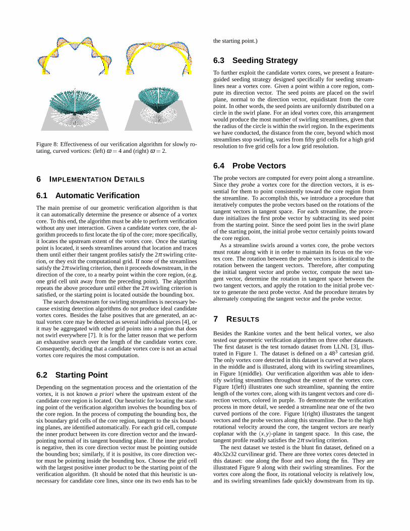
Figure 8: Effectiveness of our verification algorithm for slowly ro-tating, curved vortices: (left) ω = 4 and (right) ω = 2.

6 IMPLEMENTATION DETAILS

6.1 Automatic VerificationThe main premise of our geometric verification algorithm is thatit can automatically determine the presence or absence of a vortexcore. To this end, the algorithm must be able to perform verificationwithout any user interaction. Given a candidate vortex core, the al-gorithm proceeds to first locate the tip of the core; more specifically,it locates the upstream extent of the vortex core. Once the startingpoint is located, it seeds streamlines around that location and tracesthem until either their tangent profiles satisfy the 2π swirling crite-rion, or they exit the computational grid. If none of the streamlinessatisfy the 2π swirling criterion, then it proceeds downstream, in thedirection of the core, to a nearby point within the core region, (e.g.one grid cell unit away from the preceding point). The algorithmrepeats the above procedure until either the 2π swirling criterion issatisfied, or the starting point is located outside the bounding box.

The search downstream for swirling streamlines is necessary be-cause existing detection algorithms do not produce ideal candidatevortex cores. Besides the false positives that are generated, an ac-tual vortex core may be detected as several individual pieces [4], orit may be aggregated with other grid points into a region that doesnot swirl everywhere [7]. It is for the latter reason that we performan exhaustive search over the length of the candidate vortex core.Consequently, deciding that a candidate vortex core is not an actualvortex core requires the most computation.

6.2 Starting PointDepending on the segmentation process and the orientation of thevortex, it is not known a priori where the upstream extent of thecandidate core region is located. Our heuristic for locating the start-ing point of the verification algorithm involves the bounding box ofthe core region. In the process of computing the bounding box, thesix boundary grid cells of the core region, tangent to the six bound-ing planes, are identified automatically. For each grid cell, computethe inner product between its core direction vector and the inward-pointing normal of its tangent bounding plane. If the inner productis negative, then its core direction vector must be pointing outsidethe bounding box; similarly, if it is positive, its core direction vec-tor must be pointing inside the bounding box. Choose the grid cellwith the largest positive inner product to be the starting point of theverification algorithm. (It should be noted that this heuristic is un-necessary for candidate core lines, since one its two ends has to be

the starting point.)

6.3 Seeding StrategyTo further exploit the candidate vortex cores, we present a feature-guided seeding strategy designed specifically for seeding stream-lines near a vortex core. Given a point within a core region, com-pute its direction vector. The seed points are placed on the swirlplane, normal to the direction vector, equidistant from the corepoint. In other words, the seed points are uniformly distributed on acircle in the swirl plane. For an ideal vortex core, this arrangementwould produce the most number of swirling streamlines, given thatthe radius of the circle is within the swirl region. In the experimentswe have conducted, the distance from the core, beyond which moststreamlines stop swirling, varies from fifty grid cells for a high gridresolution to five grid cells for a low grid resolution.

6.4 Probe VectorsThe probe vectors are computed for every point along a streamline.Since they probe a vortex core for the direction vectors, it is es-sential for them to point consistently toward the core region fromthe streamline. To accomplish this, we introduce a procedure thatiteratively computes the probe vectors based on the rotations of thetangent vectors in tangent space. For each streamline, the proce-dure initializes the first probe vector by subtracting its seed pointfrom the starting point. Since the seed point lies in the swirl planeof the starting point, the initial probe vector certainly points towardthe core region.

As a streamline swirls around a vortex core, the probe vectorsmust rotate along with it in order to maintain its focus on the vor-tex core. The rotation between the probe vectors is identical to therotation between the tangent vectors. Therefore, after computingthe initial tangent vector and probe vector, compute the next tan-gent vector, determine the rotation in tangent space between thetwo tangent vectors, and apply the rotation to the initial probe vec-tor to generate the next probe vector. And the procedure iterates byalternately computing the tangent vector and the probe vector.

7 RESULTS

Besides the Rankine vortex and the bent helical vortex, we alsotested our geometric verification algorithm on three other datasets.The first dataset is the test tornado dataset from LLNL [3], illus-trated in Figure 1. The dataset is defined on a 483 cartesian grid.The only vortex core detected in this dataset is curved at two placesin the middle and is illustrated, along with its swirling streamlines,in Figure 1(middle). Our verification algorithm was able to iden-tify swirling streamlines throughout the extent of the vortex core.Figure 1(left) illustrates one such streamline, spanning the entirelength of the vortex core, along with its tangent vectors and core di-rection vectors, colored in purple. To demonstrate the verificationprocess in more detail, we seeded a streamline near one of the twocurved portions of the core. Figure 1(right) illustrates the tangentvectors and the probe vectors along this streamline. Due to the highrotational velocity around the core, the tangent vectors are nearlycoplanar with the (x,y)-plane in tangent space. In this case, thetangent profile readily satisfies the 2π swirling criterion.

The next dataset we tested is the blunt fin dataset, defined on a40x32x32 curvilinear grid. There are three vortex cores detected inthis dataset: one along the floor and two along the fin. They areillustrated Figure 9 along with their swirling streamlines. For thevortex core along the floor, its rotational velocity is relatively low,and its swirling streamlines fade quickly downstream from its tip.

Figure 9: Blunt fin dataset

Upon a closer inspection in Figure 10(top left), both the core re-gion and the streamlines exhibit a flat shape that does not resemblethe cylindrical shape of an ideal vortex. In the flat regions in Fig-ure 10(top right), the tangent vectors are nearly colinear, creatingtwo clusters in tangent space that are opposite of each other. Evenin this case, the tangent profile satisfies the 2π swirling criterion.

The last dataset we tested was the delta wing dataset fromNASA, defined on a 67x209x49 curvilinear grid, with an angle ofattack at 30. With this dataset, we can demonstrate not only theverification process for vortex cores but also the elimination pro-cess for false positives. In total, there are fourteen detected vor-tex cores in this dataset, of which six exhibit swirling motion andthe other eight do not. We attribute these eight false positives tobe artifacts of the detection algorithm. Figure 11(left) illustratesthe six vortex cores in yellow and the eight false positives in lightgreen. Figure 11(middle) illustrates the six vortex cores along withtheir swirling streamlines. For the two wing-edge vortices, our ver-ification algorithm did not identify any swirling streamlines untilreaching the middle portion of their vortex cores. Figure 11(right)illustrates the tangent vectors and probe vectors along a swirlingstreamline of the vortex core on the left wing. The tangent profileclearly satisifies the 2π swirling criterion.

Figure 12 illustrates the difference in tangent profiles between avortex core and a false positive. Whereas the top tangent profileclearly satisfies the 2π swirling criterion, the bottom one does not.The bottom tangent profile is typical of streamlines from the falsepositive: the angle spanned is less than one quadrant of the (x,y)-plane in tangent space. The slight bent in the streamlines accountfor most of the variations in the tangent profile.

8 CONCLUSION

We have presented a geometric verification algorithm for vorticalfeatures in flow fields. This algorithm addresses the need to dealwith false positives that are inevitably generated from existing de-tection algorithms. It automates the visual inspection process thathas become the defacto method for verifying detected results. With-out a formal definition, our verification algorithm proceeds to iden-tify the swirling streamlines that are commonly associated with 3Dvortices. Given a candidate vortex core, our verification algorithmautomatically searches for the swirling streamlines surrounding thecore region, where the measure for swirl is defined in terms of thedifferential geometry properties of the streamline. We have suc-cessfully demonstrated the efficacy of our approach using several

Figure 10: Despite the flatness of the vortex core region and itsswirling streamlines, its tangent profile still satisfies the 2π swirlingcriterion.

standard examples and datasets.One of the limitations of our apporoach is that it does not address

the frame of reference issue that is central to unsteady flows. Ourverification approach may encounter difficulty with vortices in un-steady flows. In our opinion, this is a difficult problem that has notbeen addressed adequately. We plan to address this issue formallyin future work, along with tracking swirling features robustly andefficiently in unsteady flows.

9 ACKNOWLEDGMENTS

We would like to thank Prof. Han-Wei Shen from The Ohio StateUniversity for providing us with the delta wing dataset. This workis partially funded by the NSF under the Large Data and ScientificSoftware Visualization Program (ACI-9982344), the InformationTechnology Research Program (ACS-0085969), a grant from theArmy Research Office (DAA D19-00-1-0155) and an NSF EarlyCareer Award (ACI-9734483). We also thank the anonymous re-viewers for many useful suggestions.

REFERENCES

[1] D. C. Banks and B. A. Singer. A Predictor-Corrector Tech-nique for Visualizing Unsteady Flow. IEEE Trans. on Visual-ization and Computer Graphics, 1(2):151–163, 1995.

[2] C. H. Berdahl and D. S. Thompson. Eduction of SwirlingStructure Using the Velocity Gradient Tensor. AIAA J.,31(1):97–103, January 1993.

[3] R. Crawfis and N. Max. Texture Splats for 3D Vector andScalar Field Visualization. In Proc. IEEE Visualization ’93,pages 261–266, October 1993.

[4] R. Haimes and D. Kenwright. On the Velocity Gradient Ten-sor and Fluid Feature Extraction. In AIAA 14th ComputationalFluid Dynamics Conference, Paper 99-3288, June 1999.

Figure 11: The delta wing dataset: (left) vortex cores in yellow and false positives in light green, (middle) vortex cores and their swirlingstreamlines and (c) verification process for the right wing vortex.

Figure 12: Difference in tangent profiles between a vortex core anda false positive.

[5] M. Henle. A Combinatorial Introduction to Topology. Dover,1979.

[6] J. Jeong and F. Hussain. On the Identification of a Vortex. J.Fluid Mechanics, 285:69–94, 1995.

[7] M. Jiang, R. Machiraju, and D. Thompson. A NovelApproach to Vortex Core Region Detection. In JointEurographics-IEEE TCVG Symposium on Visualization,pages 217–225, May 2002.

[8] Y. Levy, D. Degani, and A. Seginer. Graphical Visualizationof Vortical Flows by Means of Helicity. AIAA J., 28(8):1347–1352, August 1990.

[9] H. Lugt. Vortex Flow in Nature and Technology. Wiley, 1972.

[10] R. Machiraju, J. Fowler, D. S. Thompson, W. Schroeder, andB. K. Soni. EVITA - Efficient Visualization and Interrogation

of Tera-Scale Data. In Data Mining for Scientific and En-gineering Applications, pages 257–279. R. Grossman et al.,eds., Kluwer Academic Publisher, 2001.

[11] R. Peikert and M. Roth. The ”Parallel Vectors” Operator - aVector Field Visualization Primitive. In Proc. IEEE Visual-ization ’99, pages 263–270, October 1999.

[12] L. M. Portela. Identification and Characterization of Vorticesin the Turbulent Boundary Layer. PhD thesis, Stanford Uni-versity, 1997.

[13] S. K. Robinson. Coherent Motions in the Turbulent BoundaryLayer. Ann. Rev. Fluid Mechanics, 23:601–639, 1991.

[14] M. Roth. Automatic Extraction of Vortex Core Lines andOther Line-Type Features for Scientific Visualization. PhDthesis, Swiss Federal Institute of Technology, 2000.

[15] M. Roth and R. Peikert. A Higher-Order Method for FindingVortex Core Lines. In Proc. IEEE Visualization ’98, pages143–150, October 1998.

[16] I. A. Sadarjoen. Extraction and Visualization of Geometriesin Fluid Flow Fields. PhD thesis, Delft University of Tech-nology, 1999.

[17] I. A. Sadarjoen, F. H. Post, B. Ma, D. C. Banks, and H. G.Pagendarm. Selective Visualization of Vortices in Hydrody-namic Flows. In Proc. IEEE Visualization ’98, pages 419–422,558, October 1998.

[18] D. Sujudi and R. Haimes. Identification of Swirling Flow in3D Vector Fields. In AIAA 12th Computational Fluid Dynam-ics Conference, Paper 95-1715, June 1995.

[19] D. Thompson, R. Machiraju, M. Jiang, J. Nair, G. Craciun,and S. Venkata. Physics-Based Feature Mining for Large DataExploration. IEEE Computing in Science and Engineering,4(4):22–30, July 2002.