Geometric Unity: Author’s Working Draft, v 1.0

Eric Weinstein∗

technicalfeedback@geometricunity.orggeneralfeedback@geometricunity.org

Thursday, April 1st, 2021

Abstract

An attempt is made to address a stylized question posed to ErnstStrauss by Albert Einstein regarding the amount of freedom present inthe construction of our field theoretic universe.

Figure 1: Drawing Hands.

Contents

1 Introduction: The Problem 4

∗The Author is not a physicist and is no longer an active academician, but is an Entertainerand host of The Portal podcast. This work of entertainment is a draft of work in progresswhich is the property of the author and thus may not be built upon, renamed, or profited fromwithout express permission of the author. ©Eric R Weinstein, 2021, All Rights Reserved.

1

1.1 Strategy: Ideas over Instantiation (following Dirac) . . . . . . . . 51.2 About the Present Work . . . . . . . . . . . . . . . . . . . . . . . 61.3 From Unified Field Theory to Quantum Gravity and Back . . . . 61.4 The Twin Origins Problem . . . . . . . . . . . . . . . . . . . . . 8

1.4.1 Ehresmannian Geometry Advantages . . . . . . . . . . . . 91.4.2 Riemannian Geometry Advantages . . . . . . . . . . . . . 9

1.5 Notes On The Present Draft Document . . . . . . . . . . . . . . 10

2 Incompatibility and Incompleteness Blocking Geometric Unifi-cation 112.1 Failure of Gauge Covariance: Einsteinian Projection . . . . . . . 112.2 Failure of Gauge Covariance: Torsion . . . . . . . . . . . . . . . . 122.3 Higgs Sector Remains Geometrically Unmotivated . . . . . . . . 132.4 Geometric Unity . . . . . . . . . . . . . . . . . . . . . . . . . . . 142.5 Geometric Harmony vs Quantum Gravity . . . . . . . . . . . . . 15

3 The Observerse Recovers Space-Time 163.1 Proto-Riemannian Geometry . . . . . . . . . . . . . . . . . . . . 173.2 The Chimeric Bundle . . . . . . . . . . . . . . . . . . . . . . . . 193.3 Topological and Metric Spinors . . . . . . . . . . . . . . . . . . . 203.4 Reversing The Fundamental Theorem: The Zorro Construction . 213.5 Chimeric Spinors and Heterogeneous Spin Bundles. . . . . . . . . 223.6 The Main Principal Bundle . . . . . . . . . . . . . . . . . . . . . 24

4 Topological Spinors and Their Observation 264.1 Maximal Compact and Complex Subgroup Reductions of Struc-

ture Group . . . . . . . . . . . . . . . . . . . . . . . . . . . . . . 274.2 Pati-Salam . . . . . . . . . . . . . . . . . . . . . . . . . . . . . . 29

5 Unified Field Content: The Inhomogeneous Gauge Group andFermionic Extension 315.1 Field Content . . . . . . . . . . . . . . . . . . . . . . . . . . . . . 31

5.1.1 Field Content Native to X . . . . . . . . . . . . . . . . . . 315.1.2 Field Content Native to Y . . . . . . . . . . . . . . . . . . 31

5.2 Infinite Dimensional Function Spaces: A,H,N . . . . . . . . . . 325.3 Inhomogeneous Gauge Group: G . . . . . . . . . . . . . . . . . . 325.4 Natural Actions of G on A. . . . . . . . . . . . . . . . . . . . . . 33

5.4.1 Right Action by G on A . . . . . . . . . . . . . . . . . . . 335.4.2 Left Action by G on A . . . . . . . . . . . . . . . . . . . . 33

5.5 Fermions and SUSY . . . . . . . . . . . . . . . . . . . . . . . . . 335.6 Relationship of the Inhomogeneous Gauge Group to Standard

Analysis . . . . . . . . . . . . . . . . . . . . . . . . . . . . . . . . 34

2

6 The Distinguished connection A0 and its consequences. 356.1 The Tilted Map τ into G: the Homomorphism Rule . . . . . . . . 366.2 Stabilizer Subgroup . . . . . . . . . . . . . . . . . . . . . . . . . . 376.3 G as Principal bundle: Action by Tilted Gauge Transformations

Rule . . . . . . . . . . . . . . . . . . . . . . . . . . . . . . . . . . 376.4 Map out of G to spaces of connection: Gauge Equivariance . . . 38

7 The Augmented or Displaced Torsion 397.1 Augmented Torsion and its Transformations . . . . . . . . . . . . 397.2 Summary of spaces and maps . . . . . . . . . . . . . . . . . . . . 40

8 The Family of Shiab Operators 418.1 Pure Trace Elements . . . . . . . . . . . . . . . . . . . . . . . . . 418.2 Thoughts on Operator Choice . . . . . . . . . . . . . . . . . . . . 42

9 Lagrangians 439.1 The 1st Order Bosonic Sector . . . . . . . . . . . . . . . . . . . . 439.2 Second Order Euler-Lagrange Equations . . . . . . . . . . . . . . 459.3 The Fermionic Sector . . . . . . . . . . . . . . . . . . . . . . . . . 46

10 Deformation Complex 47

11 Observed Field Content 4911.1 Fermionic Quantum Numbers as Reply to Rabi’s question. . . . . 5011.2 The Three Family Problem in GU and Imposter Generations. . . 5011.3 Explict Values: Predicting the Rest of Rabi’s Order. . . . . . . . 5211.4 Bosonic Decompositions . . . . . . . . . . . . . . . . . . . . . . . 53

12 Summary 5412.1 Equations . . . . . . . . . . . . . . . . . . . . . . . . . . . . . . . 5512.2 Space-time is not Fundamental and is to be Recovered from Ob-

serverse. . . . . . . . . . . . . . . . . . . . . . . . . . . . . . . . . 5512.3 Metric and Other Field Content are Native to Different Spaces. . 5612.4 The Modified Yang-Mills Equation Analog has a Dirac Square

Root in a Mutant Einstein-Chern-Simons like Equation . . . . . 5612.5 The Failure of Unification May Be Solved by Dirac Square Roots. 5712.6 Metric Data Transfer under Pull Back Operation is Engine of

Observation. . . . . . . . . . . . . . . . . . . . . . . . . . . . . . 5812.7 Spinors are Taken Chimeric and Topological to Allow Pre-metric

Considerations. . . . . . . . . . . . . . . . . . . . . . . . . . . . . 5912.8 Affine Space Emphasis Should Shift to A from Minkowski Space. 6012.9 Chirality Is Merely Effective and Results From Decoupling a Fun-

damentally Non-Chiral Theory . . . . . . . . . . . . . . . . . . . 6012.10Three Generations Should be Replaced by 2+1 model of two True

Generations and one Effective Imposter Generation . . . . . . . . 6212.11Final Thoughts . . . . . . . . . . . . . . . . . . . . . . . . . . . . 63

3

1 Introduction: The Problem

“What really interests me is whether god had any choice in thecreation of the world.” -Albert Einstein to Ernst Strauss

In the beginning we will let X4 be a 4-dimensional C∞ manifold with a chosenorientation and unique spin structure. It is otherwise considered to be withouta geometry in that no metric, symplectic, complex, volume, quaternionic orother structure is yet imposed upon it. It was the original intention of [8] toconsider to what extent the opening epigrammatic question of Einstein couldbe considered a scientific program, rather than a philosophical one, by askingwhether the observed world could be extracted from little more than such initialdata as above.

Because Einstein did not specify what he meant exactly, we have taken theliberty of reformulating his question as follows:

“Starting fromX4, as the topological structure underlying the Space-Time construction, to what extent can the observed universe to-gether with stylized contents and laws mirroring its own be gener-ated without further assumptions?”

so that what we are effectively asking is whether there is a plausible map:

X4 −→

+sRicci Scalar Einstein

− 14 < FA, FA > Yang-Mills-Maxwell

+i < ψ, /∂Aψ > Dirac

+ < φ, d∗AdAφ > −V (φ) Higgs

+ < ψ, φψ > Yukawa

L= Sl(2,C) Lorentz Group

SU(3)× SU(2)×U(1) Internal Symmetries

Q = C16H Family Quantum Numbers

ψ = ⊕3a ψa Three Families of Matter

MCKM Cabibo Kobayashi Maskawa Matrix

(1.1)which recovers the fundamental or seemingly fundamental stylized aspects ofthe observed universe from which we appear to have emerged.

To be sure, this does not seek to address the well known eternal questionof “Why is there something rather than nothing?” as we are not aware of anyavailable reformulation of that question which renders it scientific rather thanreligious or philosophical. Thus, as close as we will come to that question is

“Why might we expect a world of the richness we have found throughscience and observation, to arise out of something which is minimallydetermined beyond being a low dimensional arena for the rules ofcalculus to collide with those of linear algebra.”

4

From our perspective, a fundamental theory is simply a theory that effectivelydiscourages further scientific search for a more foundational layer. Were theworld recoverable from a manifold X4 (with little more than minor additionaldata), it would not bring either physics or theology to an end by any means.It would, however move the technically minded at last away from the searchfor fundamental law and focus them instead upon the consequences of the rulesencoded leaving the search for an explanation illuminating the initial input asa purely philosophical or, perhaps, religious question.

1.1 Strategy: Ideas over Instantiation (following Dirac)

This work arises from a particular orientation which should be shared with thereader up front. At its heart, it’s belief is that most advances that are heldup for years or even decades are blocked because of confounding factors par-ticular to instantiations of the needed idea confused for being problems withthe idea itself. This perspective animates Dirac’s 1963 Scientific American ar-ticle [3] where he argues that experiment can only be used to check agreementwith the instantiation of an idea, rather than the idea itself. Dirac referencesSchrodinger’s failure to take spin into account leading to a superficial failure toagree with experiment. He could just as easily, however, been writing about hisown superficial mistake in viewing the electron and proton as anti-particles toeach other despite the obvious mass asymmetry as pointed out by Heisenberg.

In all such cases, the initial instantiations of radical physical ideas were eitherflawed in a way the underlying ideas were not, or the presentation was such thatit caused the wrong pictures to form in the minds of those who heard it. Thusour belief is that we should be following Dirac at this juncture and looking fornatural theories and not over-indexing on their initial instantiations.

Further, we have noticed something exceedingly interesting and no less odd.The tiny minority of theorists who have contributed directly to physical lawall appear to share a common quixotic focus on beauty and internal coherencerather than an immediate emphasis on formulae, instantiation and experiment.We take from this that Einstein, Dirac and Yang were not giving general adviceas to how to do physics but rather very specific advice as to how to seek newphysical law to the almost negligible subset of working theorists who mightfollow.

As such it is our contention that one should search for a theory that isgeometrically and algebraically natural and quite close to our world at a stylisticlevel (e.g. chiral, three generations, etc...). If such a theory can be found,then, given the seemingly idiosyncratic nature of the various peculiarities of theStandard Model, it is our (historically well motivated but partially unjustified)belief that it will quite likely be that initial instantiations will be confoundedby difficulties that are likely to prove inessential and thus surmountable.

5

1.2 About the Present Work

This work was begun while the author was finishing a combined Bachelor’s andMaster’s degree program at the University of Pennsylvania which ended in 1985.At the time neutrinos were not yet claimed to posses mass and there were quitepossibly 15 particles in a generation of matter under grand unified ideas likeversions of SU(5). The present theory began on the narrow hope or ‘joke’ thatin some sense if:

15 “ = ” 2( 42+4

2)

2 −1 (1.2)

as the dimension of internal Fermionic quantum numbers, then we would be inthe unique case where peculiar spinorial methods could unify the auxiliary fiberbundle Geometry of Ehresmann with the intrinsic geometry of Riemann.

1.3 From Unified Field Theory to Quantum Gravity andBack

Starting in 1984 it became common to hear from leaders of the theoreticalphysics community that theoretical or fundamental physics was not about tra-ditional unification of the kind sought for by the like of Albert Einstein. Termslike “String Theory”, “Theory of Everything” and “Quantum Gravity” replacedunification as the driving force behind the field.

The shift was a profound one. Students went from working mostly in physicalLorentzian Signature with hyberbolic equations to Euclidean signature to takeadvantage of the Atiyah-Singer index theorem. The number of dimensions con-sidered typically dropped from the physical 4 dimensions to the toy dimensionsof 2 and 3 to take advantage of complex methods and so-called Chern-Simonslike theories respectively, or to ad hoc choice of 10, 11, 12 or 26 dimensions toaccess ‘Calabi-Yau’ manifolds, Super-Strings and Super-gravity and other exoticmechanisms. The physically relevant reductive or even semi-simple symmetriesrelated to SU(3) × SU(2) × U(1) were generally replaced with simple groupslike a single SU(2) or even U(1) in isolation. The observed family structure ofthree generations of Fermions increasingly faded from interest or was pushedonto the index theory of Calabi-Yau three-folds, while investigations began toassume the presence of space-time Super-symmetry despite the existence of zeroexperimental observation for the phenomena.

In short, interest in the direct investigation of the physical world went fromthe core of physics research to a quaint backwater, as what might be termedthe “Toy-Physics era” of String Theory inspired geometric physics began.

To understand how profound the shift truly was, it is helpful to understandwhat a major keynote address sounded like in theoretical physics in 1983, justbefore the anomaly cancellation and its embrace by Edward Witten and otherString Theorists changed the entire nature of what it meant to be a theoreticianworking on fundamental physics. Today, it reads almost as an epitaph for theviews of a bygone era. Here is Murray Gell-Mann addressing assembled leaders

6

of the Theoretical Physics community at the 1983 Shelter Island II conferencejust before the split in the community mediated by the anomaly cancellation:

From Renormalizability to Calculability?

“As usual, solving the problems of one era has shown up the criticalquestions of the next era. The very first ones that come to mind,looking at the standard theory of today, are

• Why this particular structure for the families? In particular,why flavor chiral with the left- and right-handed particles beingtreated differently, rather than, say, vectorlike, in which left andright are transformable into being treated the same?

• Why 3 families? That’s a generalization of Rabi’s famous ques-tion about the muon, which I’ll never forget: ”Who orderedthat?”) The astrophysicists don’t want us to have more than 3families. Maybe they would tolerate a 4th, but no more, withmassless or nearly massless neutrinos; it would upset them intheir calculations of the hydrogen and helium isotope abun-dances. Of course, if the neutrinos suddenly jumped to somehuge mass in going from known families to a new one, thenthey would be less upset.

• How many sets of Higgs bosons are there in the standard the-ory? Well, the Peccei-Quinn symmetry, which I’ll mentionlater, requires at least 2, if you believe in that approach. Ifthere’s a family symmetry group, there may be more, becausewe may want a representation of the family symmetry group:maybe there are 6 sets of 4 Higgs bosons; nobody knows.

• Why SU(3) x SU(2) x U(1) in the first place? Here, of course,there have been suggestions. We note that the trace of thecharge is zero in each family, and that suggests unification witha simple Yang-Mills group at some high energy, or at least aproduct of simple groups with no arbitrary U(1) factors. If thegroup is simple or a product of identical simple factors, thenwe can have a single Yang-Mills coupling constant.”

-Murray Gell-Mann, 1983

Sadly, the questions raised in this keynote have not really been answered atthe time of this writing, nor have they been a particularly strong motivatingforce over the nearly 40 years that have followed this address. And with thisstagnation came a desire to change the key problems in the theory just citedto ones that would allow for great deals of activity and elaboration. Thus, theemphasis shifted to ‘Quantum Gravity’ in the following year and the search fora compelling version of quantized string theories that would recover our worldin short order. In fact, it never arrived.

7

1.4 The Twin Origins Problem

The problem of unification in physics is reasonably well appreciated by mostmembers of the research community ostensibly working on this problem. Whatis less well appreciated is the number of distinct ways unification may be inter-preted outside the dominant narrative within the field.

One way that seems to get comparatively less attention is to make use of therevolution in geometric physics that happened principally between Jim Simonsand C.N. Yang at Stony Brook in the mid 1970s where it was discovered thatclassical Ehresmannian bundle theoretic geometry was playing the same rolebeneath classical and Quantum Field Theory that Riemannian geometry wasplaying in under-girding General Relativity.

Viewed in this way, it is possibly the difference in geometric frameworksof Einstein and Bohr that are more important than the issue of quantization.Oddly, perhaps the most succinct synopsis of the main ideas in fundamentalphysics was given in 1986 by Edward Witten in a way that laid bare that ithas been the geometry of physical law rather than the quantum which hasconstituted our three greatest insights:

Figure 2: Edward Witten Synopsis.

Seen from this perspective (i) corresponds to the Einstein Field Equations ofSemi-Riemannian geometry, (ii) to the Yang-Mills generalization of Maxwell’sequations to Non-Abelian Ehresmannian gauge theory and (iii) to the Diracequation which mixes the bundle structures of both frameworks. The Klein-Gordon equation for the Higgs Fields with its iconic quartic potential is notmentioned and the quantum is clearly featured not as a rival insight, but as amethod of viewing the three main discoveries.

This raises the question: Why did we become focused on quantizing gravitywhen the underlying data given in (i) and (ii) are themselves of geometricallydifferent origins? So long as auxiliary principal G-bundles are invoked withoutcompelling justification, there is no sense in which theoretical physics will havea satisfying origin story for the universe. Why then are we not more focused

8

on the ‘Twin Origins Problem’ of why we have separate inexplicable origins forM1,3 and SU(3)× SU(2)×U(1)?

Ostensibly this is likely to be due to the pessimism that grew up around thelack of progress in Kaluza Klein type theories that sought a single origin. Butthe fact remains that what we need is not necessarily ‘quantum gravity’ butrather a means of harmonizing General Relativity with the Standard Model ina theory free of paradox. To our mind, this suggests an emphasis on tying theauxiliary data in (ii) to the fundamental substrate of (i) at the level not of thequantum but at the level of geometry to resolve the tensions between intrinsicand auxiliary bundle geometries.

1.4.1 Ehresmannian Geometry Advantages

The major advantages that Ehresmannian geometry offers to theoretical physicsis the freedom to choose the internal symmetries of a physical theory withoutbeing confined to symmetries tied to the tangent bundle of Space-time. Thisdecoupling allows physics to account for forces like the Strong and Electro-Weakforces responsible for atomic nuclei, the electron orbitals that surround them,and their decay through beta radiation respectively.

Secondarily, the ability to remove redundancy in the description of natureby restricting our attention to Gauge Invariant quantities has turned out to bea powerful tool for reasons that, at least to this author, seem not yet completelyclear. Yet some benefit is clearly gained by being able to write down expressionswhere they are most natural and then reducing them via gauge symmetry towhere they are most economical and least repetitive.

1.4.2 Riemannian Geometry Advantages

In the case of Riemannian and Pseudo-Riemannian geometries, the freedom toconsider ad hoc candidates for physical symmetries is radically restricted. Yetthere is again a major and a minor advantage.

While the full Riemann curvature tensor is a specific example of the moregeneral Ehresmannian Curvature tensor construction, its decomposition intosub-components has no general analog in Ehresmannian geometry. Thus thegreatest advantage of Einstein and Grossman’s choice of Riemannian geometryis almost certainly to replace the broad freedom lost in bundle choice with themuch more restricted freedom to play separately with the Weyl, (Traceless)Ricci, and Scalar components of the full curvature tensor as Einstein did in1915.

While that may not seem to modern field theoretic tastes like a sensibletrade-off given the loss in choice of structure, it appears sufficient for onevery particular application of great importance: gravity. Further, properly ab-stracted, the projection operators onto curvature sub-components may be seenas tensor product decompositions in such a way as to include the Dirac oper-ator on Spinors with its contraction on 1-form valued Spinors. Viewed in thisfashion, the ability to decompose tensor products of representations involving

9

the tangent and cotangent bundles is the clear enticement to work within themetric paradigm.

The way this discussion has been framed by the above is designed to suggestthe search for a parallel in the form of a second minor advantage. And herethere is room for debate. The other main attribute of Riemannian geometrythat suggests itself hides in plain sight under the label of the ‘The FundamentalTheorem’ of Riemannian geometry. The choice of a Levi-Civita connection madeby the metric is certainly convenient, but its use can always be seen as a choiceto be made dynamically by allowing more general connections as suggested byPalatini. Thus its main value is that it allows the torsion tensor of any otherconnection to be calculated by converting the affine space of connections intoan honest vector space with the Levi-Civita connection at the origin.

However, this has always led to a puzzle: what good is being able to definethe torsion tensor of a metric connection if the Levi-Civita connection is theonly one that appears to matter in practice? Thus the torsion tensor appears,potentially, to be the solution to a problem which no one has yet thought to ask.As such, its potential advantages have so far been minor with its realized onescloser to non-existent. But it must be considered to be a potential advantageas the natural answer to a question which may some day arise.

1.5 Notes On The Present Draft Document

There is something about the nature of LaTeX that is likely to confuse theprofessional reader. It is as if a typeset document constitutes agreement toparticipate in some academic social contract. No such consent is intended bythis. The author functions totally divorced from the professional research con-text which is oddly automatically inferred from typeset mathematics by nearlyevery capable reader, perhaps due to the rarity of such research programs.

Without wishing to dwell on this unduly, there is no way around the factthat the author has been working in near total isolation from the communityfor over 25 years, does not know the current state of the literature, and has few,if any, colleagues to regularly consult.

As such this document is an attempt to begin recovering a rather morecomplete theory which is at this point only partially remembered and stichedtogether from old computer files, notebooks, recordings and the like dating backas far as 1983-4 when the author began the present line of investigation. Thisis the first time the author has attempted to assemble the major components ofthe story and has discovered in the process how much variation there has beenacross matters of notation, convention, and methodology1. Every effort has beenmade to standardize notation but what you are reading is stitched together fromentirely heterogeneous sources and inaccuracies and discrepancies are regularlyencountered as well as missing components when old work is located.

The author notes many academicians find this unprofessional and thereforeirritating. This is quite literally unprofessional as the author is not employed

1The biggest issue of heterodox methodology appears to have been shifts between repre-sentation theoretic and indicial methods of tensorial and spinorial products and contractions.

10

within the profession and has not worked professionally on such material sincethe fall of 1994. If you find this disagreeable, please feel free to take yourprofessional assumptions elsewhere. This document comes from a context totallydifferent from the world of grants, citations, research metrics, lectures, awardsand positions. In fact, the author claims that if there is any merit to be foundhere, it is unlikely that it could be worked out in such a context due to theauthor’s direct experience of the political economy of modern academic research.This work stands apart from that context and does so proudly, intentionally,and without apology.

With that said, the author welcomes constructive technical feedback at:technicalfeedback@geometricunity.org and non-technical constructive feedbackat generalfeedback@geometricunity.org.

Lastly, the author notes that academicians repeatedly fail to cite, acknowl-edge or name work that does not come from within the circle of leading researchinstitutions. The author alerts the reader that these practices are widespreadwithin the academy but are generally not acceptable in the world outside academe.Constructive feedback is welcome but this should be considered as work inprogress of the author and not an invitation for cherry topping, denigration,theft, scooping or other widespread anti-social academic practices broadly tol-erated within the profession. Consult the author if this is any way confusing.

2 Incompatibility and Incompleteness BlockingGeometric Unification

It has become familiar to hear that Einstein’s theory of gravity cannot be unifiedwith the Standard Model of quantum field theory because there is no knownway to renormalize a quantum theory of metrics. However, this betrays a fo-cus on making the work of Einstein submit to the viewpoint of Bohr, thatis the signature of a group of quantum theorists who view holdouts refusingto acknowledged the supremacy of the received quantum viewpoint as invitingquantum domination. We hold with Einstein that the Quantum is indisputable,but that its instantiations and their interpretations do not carry the same infal-libility. So, for us, there are many incompatibilities between General Relativityand the classical field theory whose quantization defines the standard model.Our gambit is that if there is a natural classical field theory that strongly re-sembles the standard model together with General Relativity, then if it can beshown to emerge naturally from minimal assumptions, it is likely to be corrector close to correct and may well suggest its own preferred quantization. Thiscannot of course be proven but it is stated here as it is the governing philosophyof the work at hand.

2.1 Failure of Gauge Covariance: Einsteinian Projection

One of the curious failures of modern gauge theory is the uncomfortable accom-modation it gives to Einstein’s geometric general relativity. At first blush, a

11

theory of gravity built on curvature should be a natural fit for the concept ofbundle symmetry. For any curvature tensor of a connection on a principal-Gbundle PG, it always lives as a Lie Algebra valued 2-form:

FA ∈ Ω2(ad(PG)) (2.1)

and the Riemannian curvature R lijk is no different, lying as it does as a 2-form

valued in the so called adjoint to Vierbein bundle. In fact,

R lijk = F∇gµν ∈ Ω2(Λ2(T ∗(X))) (2.2)

for the Levi-Civita connection ∇gµν of a metric tensor gµν as

Λ2(T ∗(X)) = ad(PFr) (2.3)

for the given metric. Further, the Riemannian curvature is extremely well be-haved under gauge transformations

FA·h = h−1 · FA · h (2.4)

just as if it were any other curvature tensor.The incompatibility with gauge theory is in fact entirely due to the fact

that Einstein made essential use of a linear algebraic projection of his curvaturetensor which treated the twin appearances of Λ2(T ∗X) in the definition of theRiemannian Curvature Rlijk ∈ Ω2(X,Λ2(T ∗X)) on a common footing, whilethe gauge transformations strongly distinguish the two by acting trivially onthe copy corresponding to Ω2(T ∗X) = Γ∞(Λ2(T ∗X)) but non-trivially on thecopy corresponding to ad(PFr) = Λ2(T ∗X). This leads to the simple fact thatEinstein contraction or projection

PE : Λ2(TX)⊗ Λ2(TX) −→ S2(TX) (2.5)

fails to commutePE(FA·h) 6= (PE(FA)) · h (2.6)

with gauge transformations h.Curiously, this failure is often covered over by many wishing to shoehorn

General Relativity into the gauge theoretic paradigm by asserting that the dif-feomorphism group of ‘General Coordinate Transformations’ is somehow theGauge Group ‘H’ of GR, while the space of Metrics parameterizes the relevantspace of Levi-Civita Connections ‘A’ resulting in a weak version of A/H. Givenwhat we take to be the self-evident artificiality of such claims, we merely notethem here and will not dwell on them further.

2.2 Failure of Gauge Covariance: Torsion

In an explicitly trivialized coordinate patch, the covariant derivative ∇A cor-responding to a connection A can be given by specifying the connection as an

12

ad-valued 1-form A relative to the trivial connection d coming from the trivial-ization by abuse of language. This leads to the transformation formula:

h−1 (d+A) h = d+ h−1 ·A · h︸ ︷︷ ︸Gauge Covariant

+ h−1 · (dh)︸ ︷︷ ︸Gauge Non-Covariant

(2.7)

highlighting that the portion of A which is peculiar to the connection is in factgauge covariant while the portion peculiar to the trivialization lends a diseaseof gauge non-covariance to all connections which has no dependence on theconnection A at hand.

In the absence of a trivialization, but the presence of a prefered connectionA0 such as the Levi-Civita connection Ag = A0, we can write:

h−1 ∇A h−∇0 = h−1 (∇0 +A) h−∇0 (2.8)

= h−1 A h + h−1 ∇0 h = h−1Ah︸ ︷︷ ︸Connection Specific

+ h−1(d0h)︸ ︷︷ ︸Common Disease

to see that again part of the transformation law is well behaved while the dis-eased term is dependent only on the exterior derivative d0 = dA0 coupled to thedistinguished connection.

The problem here can be seen instantly if one tries to naively include thegauge potential A directly in a Lagrangian or action I:

I(A) = ||A||2 =< A,A > (2.9)

so that under a gauge transformation h we have:

I(A · h) = ||A · h||2 =< A · h,A · h > (2.10)

=< h−1Ah+ h−1dh, h−1Ah+ h−1dh >

= ||h−1Ah||2︸ ︷︷ ︸Gauge Invariant

+ ||h−1dh||2︸ ︷︷ ︸Common Disease

+ 2 < h−1Ah, h−1dh >︸ ︷︷ ︸Gauge Potential-Specific Disease

leading to a failure of gauge invariance due to both a shared and idiosyncraticterm spoiling the action under symmetry. Typically, the response to this is toavoid putting the potential into the action directly and to work instead withthe better behaved curvature tensor derived from the 1-forms in the case ofthe Standard Model, or to give up on gauge invariance at the bundle level (i.e.Einstein’s compression of Riemann’s curvature tensor) and use the action topenalize the torsion into vanishing (i.e. the Palatini action).

2.3 Higgs Sector Remains Geometrically Unmotivated

For most of the 20th century, fundamental physics was split into two halves,only one of which was geometric. Then, in the mid 1970s, the quantum sectorwas discovered to have a basis in differential geometry with the advent of theWu-Yang dictionary of Simons, Wu and Yang. Gauge potentials corresponded

13

to the geometer’s notion of a connection and Fermi fields fit with Atiyah andSinger’s rediscovery of the Dirac operator in a bundle theoretic context.

After that point, fields of fractional spin, spin 1 and spin 2 were all well mo-tivated in either Ehresmannian or Riemannian geometry. This left the curiouscase of the spin 0 Higgs sector with its so-called Mexican Hat potential. Whilethe Higgs sector could be described bundle theoretically, it was not fully naturalfor geometers to consider a spinless field valued in a Lie Algebra and governedby a quartic potential, despite the seemingly geometric nature of the MexicanHat shape.

2.4 Geometric Unity

This leads us finally to the question of the motivating concept(s) behind Geo-metric Unity.

In essence, there is both a scientific basis and a human basis rooted inpolitical economy. The scientific basis is the more important of the two andproceeds as follows.

Mapping out the various reasons that Riemannian and Ehresmannian ge-ometry have continued to progress side by side reveals that there is a trade-offto be had between the two. In the case of Ehresmannian geometry, the leadingadvantage has to be the freedom to accommodate any observed field contentfound through experiment through the use of auxiliary bundles structures. Asa compensating secondary advantage, the use of the gauge group to simultane-ously transform the field content together with the derivative structures whichfurnish the differential equations that govern propagation allows us to considera greatly reduced set of truly distinct configurations without being overwhelmedby unnecessary redundancies that we would face in the group’s absence.

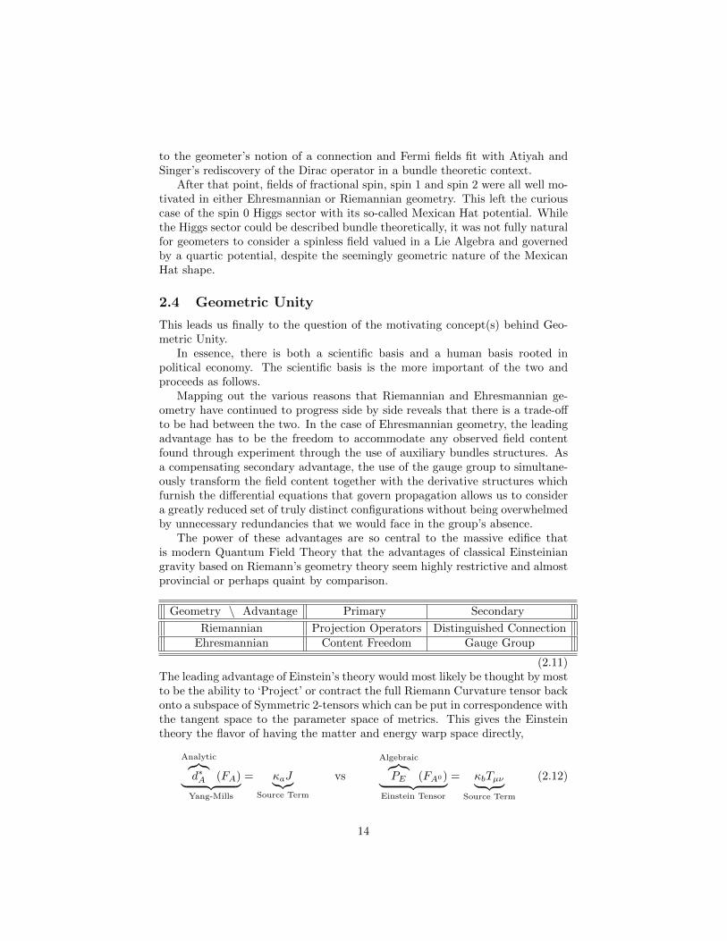
The power of these advantages are so central to the massive edifice thatis modern Quantum Field Theory that the advantages of classical Einsteiniangravity based on Riemann’s geometry theory seem highly restrictive and almostprovincial or perhaps quaint by comparison.

Geometry \ Advantage Primary Secondary

Riemannian Projection Operators Distinguished ConnectionEhresmannian Content Freedom Gauge Group

(2.11)The leading advantage of Einstein’s theory would most likely be thought by mostto be the ability to ‘Project’ or contract the full Riemann Curvature tensor backonto a subspace of Symmetric 2-tensors which can be put in correspondence withthe tangent space to the parameter space of metrics. This gives the Einsteintheory the flavor of having the matter and energy warp space directly,

Analytic︷︸︸︷d∗A (FA)︸ ︷︷ ︸

Yang-Mills

= κaJ︸︷︷︸Source Term

vs

Algebraic︷︸︸︷PE (FA0)︸ ︷︷ ︸

Einstein Tensor

= κbTµν︸ ︷︷ ︸Source Term

(2.12)

14

rather than a change in the curvature represented by a differential operatorproviding the link. This however pays a high price in that it treats the twocopies of Λ2 in Λ2⊗Λ2 where the Riemann curvature tensor lives symmetricallywhile the gauge group acts only on the second factor. This seemingly negatesmuch of the advantage of working within the Riemannian paradigm if one isinterested in harmonizing GR with QFT.

There is however a small hope. If one can give up the freedom of being ableto choose auxiliary gauge content as needed in the hopes of avoiding the doubleorigin problem, then it may be possible to work within an extremely narrow classof theories which are amenable to the advantages of both geometries. But suchgeometric frameworks are likely to be extremely restrictive. Thus one musthope that the Standard Model and General Relativity would be of a highlyunusual and non-generic geometric variety. And the main hope here is thatobserved quantum numbers of (ii) and (iii) that have no explanation withinWitten’s point (i) seem to us to be highly suggestive that the Standard Modelwith its three generation and 16 particle per generation structure is of exactlythe non-generic theory that carries both attributes.

This brings us to the less scientific and more human point. Let us askthe question whether the incentive structures of physics select for or againstthe search for a highly specific and restrictive class of geometries on whichto focus. Attempts to find such a class are likely to fail, be considered asnumerological and quixotic, and be career limiting. As such, leading physicistswould likely avoid such theories in favor of flexible frameworks which do notpaint the investigator into a research corner. To a seasoned investigator, tradinggauge invariance of the action and the freedom to choose field content to fitthe needs of a problem for mere Einstein projection maps and a distinguishedconnection, is likely to seem akin to a naive Magic Beans trade where somethingof great value is bartered away for something of obviously lesser or even dubiousimportance. Here that trade is auxiliary content freedom and gauge covariancefor contraction operators and a distinguished choice of connection.

It is the assertion here that this is not only an advantageous trade but likelya necessary one. That is, we do not need auxiliary freedom because of our goodfortune in the Standard Model, and we can buy back the gauge invariance afterexploiting the riches of projection operators and the choice of a distinguishedconnection.

2.5 Geometric Harmony vs Quantum Gravity

It is frequently stated that Gravity has to be quantized because of the paradoxthat since every particle creates a gravitational field, a classical localizationwould ultimately have to be as uncertain as the quantum particle’s locationunder observation.

In fact, this presupposes that the answer will be found in the simple Ein-steinian space-time paradigm where the argument is maximally persuasive.However, even here, there is a significant issue that is often glossed over.

Because the group Gl(4,R) does not carry a finite dimensional copy of the

15

fractional spin representations, if we allow the space time metric to become un-certain, we find a profound puzzle in the fractional spin fields. While the Spin-1force particles and Spin-0 Higgs fields may be difficult to measure between met-ric observations, the bundles in which they live are well defined in the absenceof a definite choice of metric. This however is not true for fractional spin fields.Should the metric ever successfully be ‘quantized’ in a manner similar to theother fields, there will be no finite dimensional bundle for the hadrons and lep-tons during the period between observations. Not only do the waves becomeuncertain but the media in which the waves would live would appear to be un-certain or even said to vanish. One of the goals of GU is to ensure that thebundles for spinors and Rarita-Schwinger matter do not vanish in the absenceof a metric.

By the above reasoning, We find the argument that gravity must be somehowharmonized with quantum fields in an as yet unspecified way more persuasivethan the argument that metric gravity must be quantized on the same footingas the other fields. Thus, whether gravity is to be harmonized or quantized,it is the goal of GU to decouple the existence of the fractional spin bundles asthe medium for matter waves from the assumption of a metric in the ultimatequantum theory.

3 The Observerse Recovers Space-Time

In order to make progress beyond modern General Relativity and QuantumField Theory, it is a contention of the author that Space-Time itself should besacrificed from the outset as being fundamental. As such, in Geometric Unitywe will proceed without loss of generality to consider not a single space, butpairs of spaces linked by maps. The three main cases will be defined accordingto:

Definition 3.1 An Observerse is defined to be a triple (Xn, Y d, ι) suchthat

ι : Unx −→ Y dg (3.1)

are maps for local open sets Unx ⊂ Xn about some points x ∈ Xn

constituting local Riemannian embeddings for neighborhoods Un intoa Riemannian manifold Y d of equal or higher dimension inducing apull back metric gX = ι∗(gY ) and defining a normal bundle Nd−n

ι ⊂T (Y ) with metric and its pull back ι∗(Nd−n

ι ) over Xn. The main casesof this construction correspond to:

• TRIVIAL: The manifold Y = X and the map ι is the identity.

• EINSTEINIAN: The manifold Y = Met(X) is the bundle ofpoint-wise metric tensors over X and the maps ι = g underscrutiny are sections of this bundle representing Riemannian orSemi-Riemannian metric fields.

16

• AMBIENT: The manifold Y dg is unconstrained beyond the con-dition of being an immersion.

where the first is presented to cover the case of ordinary space-timeswithout additional structure, and the last is included so as to allow forfull generality. In this work we will consider the strongest assumptionbeyond those of Einstein by working within the Einsteinian Obser-verse to search for new physics. Note that in this case, Y doesn’tusually have a pre-existing metric. Instead the choice of a section ιof the metric bundle induces a metric on Y in the portion of Y thatlies above U ⊂ X.

One reason for introducing the concept of the Observerse is to allow a morefundamental role for observation and measurement. Both of these issues havebeen at the heart of confusions in relativistic observation and Quantum Mea-surement and their as yet unsatisfactory treatment has lead some physicists toclaim that paradoxes can only be solved with a quantized gravity on par withthe other fields. Our approach is different. By working with two spaces bridgedby maps, we allow for the idea that not all fields are on par with each other andmay need to be treated differently in the fully quantized theory.

To this end we will distinguish fields according to the following:

Definition 3.2 A field χ that originates as the section of a bundle over Xn orY d will be called NATIVE to Xn or Y d respectively. Fields on X of theform ι∗(χ) will be called INVASIVE to X if they are pulled back fromfields or jet bundles χ that are native to Y .

It is our contention in this investigation that physics may actually be happeningmostly on Y d but that it is widely interpreted by physicists via metric pull-backas if it were occurring natively on Xn leading to confusion. In fact, in thisinvestigation, there will only be one independent field that is truly native toXd. This allows for the possibility that in a complete theory one could treatthe observing field on X differently from the more readily quantized fields onY without immediately leading to paradox. Different observations via differentsections ι would pull back different quantized values from Y onto X.

3.1 Proto-Riemannian Geometry

The bundle of point-wise metrics has some curious elementary properties thatmay be well known to others, but which the author did not encounter whileworking in mathematics. As might be expected, there is a tension betweenthe fact that the bundle is filled with metric information by construction, buterected without reference to any metric in particular. Thus it is chimeric in thatit is in tension between both its topological and geometrical natures.

One way of noting this intermediate state is to notice that true geometriesof both Riemannian and Symplectic type induce isomorphisms between thetangent and cotangent bundles.

17

In the presence of either a metric or symplectic form on a vector space W , weinherit a pair of canonical vector-space isomorphisms that are not canonicallydetermined in the absence of this geometric structure:

W −→W ∗ W ∗ −→W (3.2)

leading to two exact sequences:

0 T T ∗ 0 (3.3)

which, while rather trivial, suggest generalization in our case.For the Einsteinian Observerse and its Tangent and Co-Tangent bundles

TY, T ∗Y we likewise have natural and non-trivial maps:

T (Y ) −→ T ∗(Y ) T ∗(Y ) −→ T (Y ) (3.4)

However, neither of these maps is an isomorphism as they have non-trivialkernels. These can be fit into a repeating long exact sequences

. . . −→ T −→ T ∗ −→ T −→ T ∗ −→ . . . (3.5)

evidencing the relationship of a metric Chimeric bundle C(Y ) = C∗(Y ) to thepartial isomorphisms between T (Y ) and T ∗(Y ) as we shall now explain.

There exists a commutative diagram

0 0 0 0↓ ↑ ↓ ↑

. . . −→ V V ∗ −→ V V ∗ −→ . . .↓ ↑ ↓ ↑

. . . −→ T −→ T ∗ −→ T −→ T ∗ −→ . . .↓ ↑ ↓ ↑

. . . H −→ H∗ H −→ H∗ . . .↓ ↑ ↓ ↑0 0 0 0

(3.6)

where all vertical sequences are short exact and the repeating central horizontalsequence is long exact with all other maps not covered in the preceding aremetric isomorphisms.

The bundle H∗ is defined to be

H∗ = π∗(T ∗(X)) H∗ → T ∗(Y ) (3.7)

which at the point g ∈ Y carries an induced metric g via Hπ∗(π∗(g)) as the pullback of the push-forward metric. We will refer to the dual bundle (H∗)∗ simplyas H.

Conversely, as a fiber bundle, the total space Y carries a vertical sub-bundleV ⊂ T (Y ) as the subspace of vectors pointing along the fibers of Y over X.Here again, the structure of Y as a space of metrics becomes germane.

18

At a point y ∈ Y , lying in the fiber π−1(π(y)) let two symmetric two tensorsA, B ∈ TVy (X) represent a random choice of two elements in the vertical tangentspace along two different smooth paths of non-degenerate metrics gA(t), gB(t)where at time t = 0 we have gA(0) = gB(0) = y with gA(t) = A and gB(t) = B.Then, by the symmetry of the metrics, the Frobenius inner product is definedby the double contraction against the metric represented by the point y which,in an orthonormal basis would look like:

< A,B >y= Try(AT ·B) = Try(A ·B) (3.8)

were the tensors A,B represented as matrices in that basis. Here the space ofmetrics breaks into a Trace and Traceless component. The Traceless component

has signature (i ·n− i2, n2+2i2−2i·n+n−2

2 ) with a freedom to assign either a (0,1)or (1,0) signature to the trace component. In this exposition we choose the laterso as to assume our Frobenius metric can be taken to be of signature

(i · n− i2 + 1,n2 + 2i2 − 2i · n+ n− 2

2) = (4, 6) for i = 1, n = 4 (3.9)

for the four dimensional (1, 3) metric of greatest physical interest with one tem-poral and three spatial dimensions. Naturally, this would work equally well fora cosmetic shift to the (3, 1) sector, but we are treating the 3-spatial and 1-temporal dimension as anthropically determined in either case and would imag-ine that the other sectors carry physical reality disconnected from our sector.2

3.2 The Chimeric Bundle

We now define two metric bundles which, with the above assignments, are canon-ically isomorphic:

C(Y ) = C = V ⊕H∗ C∗(Y ) = C∗ = V ∗ ⊕H (3.10)

where each of these Chimeric bundles may be thought of as ‘semi-canonically’equivalent to the Tangent and Co-Tangent bundles according to:

C∗

T T↑ ↓T ∗ T ∗

C

(3.11)

as one way of formally linking two short exact sequences.These bundles C = C(Y ) and C∗ are distinguished by the fact that they

are (semi-canonically) isomorphic to the tangent bundle in the case of C and

2NB: This choice is one of the few non-forced choices allowed in the strong form of GU.

19

the co-tangent bundle in the case of C∗ and possess natural metrics. Becausethe fibers at a point g ∈ Y impart metrics to to the vertical Vg and horizontalsub-bundles H∗g , taking those sub-spaces to be orthogonal to each other allowsfor two different choices of metric to be inherited by their direct sum accordingto choices of sign.

3.3 Topological and Metric Spinors

What then is the purpose of defining bundles that are isomorphic to T and T ∗

but with only part of that isomorphism being canonical?The answer lies in the paradox of Spinors. While the Dirac operator may

well carry topological information that is not metric, it is usually impossible todefine a natural finite dimensional bundle of spinors on Xn in the absence of ametric, even when one can lift the General Linear group to its connected two-fold double cover GL(N,R), due to the absence of finite dimensional fractionalspin representations.

By passing to Y d however, we can do somewhat better by virtue of the factthat spinor representations carry an exponential property. That is, the spinorfunctor converts direct sums of vector spaces as input into tensor products ofspinor representations as output:

/S(Wa ⊕Wb) ∼= /S(Wa)⊗ /S(Wb) (3.12)

At the bundle level, we apply this to the metric Chimeric Bundle at a pointg ∈ Y to obtain:

/Sg(C) ∼= /Sg(V ⊕H∗) ∼= /SFrobeniusg

(V )⊗ /Sg(H∗π∗(π∗(g))

) (3.13)

which gives spinors defined for the metric endowed C = C∗ without making achoice of metric on Y .

This is important for several reasons. In the first place, we have defined aSpin Bundle for the chimeric bundle C(Y ) which is semi-canonically isomorphicto metric bundles of spinors on TY . Thus at the cost of replacing X with thetotal space of a natural bundle over it, we have come rather close to definingspinors without a choice of metric via maps:

TY

0 −→ C ⊕ C∗ −→ 0

T ∗Y

(3.14)

More importantly, we must have in the back of our minds that we are ultimatelygoing to have to harmonize gravitation and the metric with fractional spin Fermifields which depend on that tensor for their existence. This construction allowsus to work with one single bundle of spinors even when there is no choice ofmetric. When a metric is chosen below on X compatibly with V and H, the

20

Chimeric bundle and Tangent are given a natural isomorphism via the Levi-Civita connection

/S(V )⊗ /S(H)︸ ︷︷ ︸Topological Spinors

−→ /S(T ) = /S(T ∗)︸ ︷︷ ︸Metric Spinors

(3.15)

telling us how the Horizontal bundle H maps into TY . This in turn clearsthe way to allow us to later consider quantum Fermi fields which usually carrymetric bundle dependence between invocations of metric tensors.

3.4 Reversing The Fundamental Theorem: The Zorro Con-struction

According to the fundamental theorem of Riemannian Geometry, every Rieman-nian or (semi-Riemannian metric) induces a unique metric compatible torsionfree Levi-Civita connection on its tangent bundle.

As we have two spaces, X,Y , this is equally true both above and below inour construction of the Observerse:

Metrics Connections

On X ג −→ ℵג

On Y g −→ Ag

(3.16)

However, what is necessary to split the cyclic long exact sequence of mapsbetween T and T ∗ is in fact a connection on the space Y viewed as a bundleover X. By reversing the usual logic somewhat and linking these two maps, weget a train of transmission where a metric choice below on X leads ultimatelyto the choice of a connection above over Y :

Metrics Connections

On X ג −→ ℵג

On Y gℵ −→ Ag

(3.17)

The importance of this is that each observation of Y via a choice of metric ג onX actually induces a metric and connection on Y identifying the Topologicalspinors with the metric spinors. This allows us somewhat more confidence toexplore the idea that metrics are not even necessarily present on Y unless whenobserved where the act of observing under pull back .∗ג Further, if the problemwith much of quantum gravity turns out to be the difficulty of quantizing metricsrelative to other fields such as vector potentials, this excercise allows us tomove to more conducive variables for those who harbor dreams of quantizinggravitation.

21

It should be pointed out here that most possible metric on Y are neverin play. The subset of metrics that we are considering are incredibly tightlyconstrained and are equivalent to the space of connections that can arrise on Xas Levi-Civita connections, as opposed to the space of all metrics over Y . Thusthe issue of what upstairs gravity waves are possible doesn’t arise as the spaceof relevant fields is downstairs on X.

3.5 Chimeric Spinors and Heterogeneous Spin Bundles.

Now that we have abstractly defined spinor bundles on Y , it behoves us tounderstand what kind of spinors we may have coaxed into existence.

We should begin by noting that the choice of (1, 3) metric signature (whichcan be mirrored by choice of a (3, 1) and thus is not meaningfully distinguishedfrom it) is treated by us as anthropic data. If it were otherwise, there wouldlikely be no life to evolve to observe these structures. This recognition, forcesa (3, 6) signature on the space of traceless symmetric two tensors which, whencombined with the trace portion seen as either a (0, 1) or (1, 0) space, canbecome either a (3, 7) or the (4, 6) metric respectively. Here again, we make ananthropic choice and select the latter of the two for two reasons. In the firstplace, we believe that (3, 7) will not be compatible with the observed forces andsymmetries of the Standard Model. Secondly, we want to leave ourselves roomfor complex techniques and view a real (4, 6)R structure as holding the dooropen for some models we have been playing with favoring reduction to (2, 3)C.

Lastly we must combine these choices of fiber metrics in Y with metricspulled up from the base space of signature (1, 3). These combinations in turncould lead to (4, 10) or (8, 6) in the discarded former cases of (7, 3) or (3, 7),or (5, 9) or (7, 7) in the case of the latter (4, 6) or (6, 4). We do not know howto choose between these however as this is one of the few places in the modelwhere choices are made that are not yet forced.

To begin with, we will assume that the metric on Y is split with signature(7, 7) (rather than (9, 5) which can be worked out by the interested reader) asit is more balanced and appears to lend itself better to both some complex andClifford Algebra techniques.

Here the split signature Clifford algebra is of Real type and is equivalent toReal 128 square matrices with some additional structure:

Cl7,7 ∼= R(128) (3.18)

This in turn leads to representations for the Spin group of the form:

Spin(7, 7) −→ SO(64, 64) −→ U(64, 64) (3.19)

so in full generality, all spin representations in (7, 7) signature are subsumed by:

ρSpin : Spin(14,C) −→ U(128,C) (3.20)

The additional structure on these matrix algebras gives them a transposeoperation from combining the canonical automorphism of the Clifford algebras

22

(by replacing the generating tetrad with its negative) and the canonical anti-automorphism gotten from reversing the order of basis factors within the variousClifford products.

This leads to concrete models for a number of Lie algebras at the level ofClifford Algebras as in:

so(7, 7) “ = ” Λ2 ⊂ ClR(7,7) (3.21)

gl(64,R) “ = ” (Λ2 ⊕ Λ6 ⊕ Λ10 ⊕ Λ14) ⊂ ClR(7,7) (3.22)

As the Left and Right real Weyl spinors transform as 64-dimensional dual defin-ing representations under the General Linear group GL(64,R), we can form ametric on the space of total Majorana Spinors

/SR = /SLR ⊕ /S

RR = /S

LR ⊕ (/S

LR)∗ (3.23)

according to< ψL + ψR, σL + σR >= ψL(σR) + σL(ψR) (3.24)

giving us a split signature metric in which both spaces of Weyls spinors are nullas for Weyl Spinors we have:

Structure Group︷ ︸︸ ︷Spin(7, 7) −→

Weyl-Left︷ ︸︸ ︷Gl(64,R)+×

Weyl-Right︷ ︸︸ ︷Gl(64,R)− −→

Dirac︷ ︸︸ ︷Gl(128,C) (3.25)

The metric for the total Majorana spinors corresponds to the Lie Algebra:

so(64, 64) “ = ” (Λ2 ⊕ Λ6 ⊕ Λ10 ⊕ Λ14)︸ ︷︷ ︸/SL⊗/SR=/SL⊗/S

∗L=/S∗R⊗/SR

⊕ (Λ1 ⊕ Λ5 ⊕ Λ9 ⊕ Λ13)︸ ︷︷ ︸Λ2(/SL)⊕Λ2(/SR)

⊂ ClR(7,7)

(3.26)corresponding to the non-compact real group Spin(64, 64) ⊂ ClR(7, 7).

In order to move from Orthogonal to Unitary representations3, we pass tothe Clifford Algebra ClC(7, 7)

u(64, 64)“ = ”

3⊕i=0

Λ4i+23⊕i=0

iΛ4i3⊕i=0

Λ4i+12⊕i=0

iΛ4i+3 ⊂ ClR(7,7) ⊗ C (3.27)

corresponding to the Lie Group H = U(64, 64), where the ‘adjoint’ operationin the Clifford Algebra is given by the operation of composing the canonicalautomorphism with the reversal of order of all basis vectors.

By exponentiation we arrive at a unitary representation

ρDiracC : Spin(7, 7) → U(64, 64) (3.28)

of the Spin group into a space of unitary Dirac Spinors whose corresponding LieAlgebra is in canonical correspondence with the exterior algebra inside ClC(7, 7).

3This decomposition was taken from a decades old file and should be checked by someonemore current on their “Clifford Checkerboard” yoga as it did not come with a description.

23

3.6 The Main Principal Bundle

We have always found the byzantine intricacies of Clifford Algebras confusingand an attempt to recollect the various containments just discussed is offeredhere:

Gl(128,C)

U(64, 64) GL(128,R)

O(64, 64) GL(64,R)L ×GL(64,R)R

Gl(64,R)↑

Spin(7, 7)(3.29)

where we are privileging one particular path up the diagram that contains themetric and unitary representations:

Spin(7, 7) −→ SL(64,R) −→ SO(64, 64) −→ U(64, 64) −→ GL(128,C) (3.30)

It is now our aim to specify the main principal bundle in finite dimensionswith which we will be working.

For the rest of this exposition, we will let %Dirac = %D be the representation

%Dirac = %D : Spin(7, 7) −→ U(64, 64) (3.31)

on complex Dirac Spinors using the notation H = U(64, 64) in what follows.4

Our main object of focus, will be taken to be:

PH = PFr(C7,7) ×%D H (3.32)

where PFr(C7,7) is the double cover of the frame bundle of the Chimeric bundle.

PH ← U(64, 64)π ↓Y 7,7 ← GL(4,R)/Spin(1, 3)π ↓X4

(3.33)

with the associated bundles:

ad = ad(PH) = PH ×ad u(64, 64) = PH ×ad h (3.34)

Ad = Ad(PH) = PH ×Ad U(64, 64) = PH ×Ad H (3.35)

/S = PH ×%D C64,64 = PH ×%D /S (3.36)

4Note: The symbol H is being used to denote two different objects. A group and ahorizontal vector space. This is unfortunate and may be rectified in future drafts.

24

Now the important thing to notice about this construction is that while it looksgeometric in nature due to the presence of Spin groups and representations, itis in fact purely Topological as no metric has been chosen. In fact, all that hasbeen chosen is the signature of a (1, 3)-metric and one can avoid even this byworking over all 5 distinct sectors (i, 4− i)4i=0 on X4 and merely noting thatwe happen to appear to exist within one of them carrying a Lorentz signatureby anthropic reasoning.

We may fairly ask what a topological /S(CY ) Spinor looks like when ‘ob-served’ from X4. The concept of an observation is of course built into thedefinition of the Observerse as a map ι observing Y from X via pullback.

ι : U −→ Y U ⊂ X4 (3.37)

and so here is naturally given by a section over a local neighborhood U ⊂ Xwhen Y fibers over X. Thus we have:

/SPH ← C64,64

π ↓Y 7,7 ← GL(4,R)/Spin(1, 3)

π ↓↑ ιUU4

(3.38)

where the key to understanding the topological spinors from the perspective ofU ⊂ X observing Y via ι is worth disentangling due to the multiplicity of rolesplayed by ιU .

In the first place ιU is a local immersion as well as a section so it constitutesan embedding of X into Y seen as an ambient space. As such, it pulls backall bundles over Y just as it pushes forward the tangent bundle of U ⊂ Xin non-degenerate fashion. When it pulls back the Tangent Bundle TY as anembedding, it splits via:

ι∗(TY ) = TU ⊕Nι = TU ⊕ TY/ι∗(TU) (3.39)

where Nι is the normal bundle of the observation. But the act of observationalso gives a splitting of the long exact sequence from before over U ⊂ X:

. . . T T ∗ T T ∗ . . . (3.40)

Including this splitting into the earlier large commutative diagram

0 0 0 0↓ ↑ ↓ ↑

. . . ↔ V V ∗ ↔ V V ∗ ↔ . . .↓ ↑ ↓ ↑

. . . T T ∗ T T ∗ . . .↓ ↑ ↓ ↑

. . . H ↔ H∗ H ↔ H∗ . . .↓ ↑ ↓ ↑0 0 0 0

(3.41)

25

we start to see the full effect of a choice of ι, as it simultaneously plays thefollowing roles:

• Observer as a generator of pullback data via ι∗.

• Ambient Embedding generating a Normal Bundle Nι.

• (Downstairs) Metric as a section of the bundle of metrics.

• Splitting of the long repeating sequence.

• Connection as can be seen as being determined via either the Zorrodiagram, the Levi-Civita Construction, or the splitting diagram above.

• (Upstairs) Metric Via the Zorro diagram.

• Isomorphism generator:

C = C∗ = TY = T ∗Y V = V ∗ = Nι = N∗ι H = H∗ = TX = T ∗X(3.42)

so that its introduction has a fairly violent effect in moving us from topologyto true geometry. Curiously, it is the only primary field in the theory that istruly native to X. As such we will use Hebrew letters gimel (ג) and aleph ℵ anddenote our immersion ι in the Einsteinian Observerse by ι = ג and its associatedconnections by ℵג to remind ourselves of the separation between fields native toX and those arising naturally on Y .

4 Topological Spinors and Their Observation

The appearance of topological spinors may then finally be interrogated underobservation by .∗ג Let x ∈ U ⊂ X be a point in the neighborhood of a localobservation Uג .

If ΨגU (x) ∈ /S(C) is a topological spinor, then under an observation by ∗ג onX it will appear as

ΨגU (x) ∈ /Sx(TX)︸ ︷︷ ︸Space-Time Spinors

⊗ /Sx(Nג(x))︸ ︷︷ ︸‘Internal’ Quantum Numbers

(4.1)

so that an observer may be lead into error. While the topological spinor underobservation is not generated by any algebraic auxiliary data unconnected to X,it is quite likely to appear as if it contains auxiliary internal quantum numbers ifthe observer is unaware of the Observerse structure involving Y , as the pull backfields via ∗ג would have the false appearance of being native to X. A tell talesign that one might be looking at such a unified structure with a single origin inX would be the presence of a power of 2 in the dimension count of the auxiliaryquantum numbers for /Sx(Nג(x)). Specifically, on an even dimensional manifold

26

of signature (i, j) = n we would expect to see internal quantum numbers ofdimension

Dim( /Sx(Nג(x))︸ ︷︷ ︸‘Internal’ QN

) = 2i2+j2+2ij+i+j

4︸ ︷︷ ︸Dirac

or 2i2+j2+2ij+i+j−4

4︸ ︷︷ ︸Weyl

(4.2)

depending on whether the theory was non-chiral (Dirac) or either effectively orfundamentally chiral (Weyl). In particular, we might expect the later in regionsU ⊂ Xi,j where gravity and curvature are weak and the former where they arestrong and resistant to effective decoupling. And, to our way of thinking,

2i2+j2+2ij+i+j−4

4︸ ︷︷ ︸Weyl

= 212+32+2∗1∗3+1+3−4

4 = 16C (4.3)

this, with a doublet of charged and uncharged leptons together with a tri-coloredpositively charged quark and its negatively charged weak isospin doublet part-ners along with the anti-particles of all the preceding, appears to be exactlywhat we see repeated over three apparent low energy families.

Lastly, we note from personal communication that Frank Wilczek appearsto have wondered about the spinorial coincidence (even in print), but did notfind it compelling enough to pursue beyond noting its existence and the lack ofincorporation within a physical framework. It is our hope that recognizing that

Figure 3: Wilczek On Internal Spinors.

the ‘10’ implicit within both the Georgi-Glashow and Pati-Salam theories maybe tied to the 10 coupled equations of General Relativity may be consideredcompelling.

4.1 Maximal Compact and Complex Subgroup Reductionsof Structure Group

Assume for the moment that we have a global observation:

ג : X −→ Y (4.4)

27

or, in our case, simply that we have a given metric on X. The push-forwardmap induced on the tangent bundle TX given by

Dג : TX −→ TY (4.5)

splits the tangent bundle on Y along (X)ג ⊂ Y into the image of Dג and its 10dimensional complement V 10 along the fiber of metrics for every x ∈ X. Thiscreates an identification with the chimeric bundle C = V10 ⊕H∗4 as the verticalpiece is already a subset of both TY and C by construction, and Im(Dג) =(H4

∗(xג

Having seen that the natural break down of our Chimeric Spin(7, 7) bundleunder observation leads to a decomposition into tangent and normal compo-nents of dimensions 4 and 10 respectively, it is natural to ask what reductionsof structure group are most natural to expect. Two immediately suggest them-selves.

Given any normal bundle that is even dimensional, there is a natural questionas to whether it admits a complex or quaternionic structure. Here the dimen-sion 10 being equal to 2 mod 4 suggests seeking a complex structure throughreduction of structure group to U(3, 2) ⊂ Spin(6, 4).

Conversely, given the non-compact nature of Spin(6, 4) it is natural to won-der whether the structure group breaking to a maximal compact subgroup withbetter stability behavior is advantaged. Thus while non-compact groups arecertainly considered from time to time, if the subgroup was broken to a max-imal compact sub-group, we would be anthropically screened from seeing hownature accommodates non-compact symmetry and thus without guidance as tohow to find a theory which extends to the general case.

To this end, we might also consider both reductions simultaneously and askhow a reduction to a maximal compact subgroup would appear if it were accom-panied by a simultaneous reduction to accommodate a 5 complex dimensional

28

normal bundle. Starting from Spin(1, 3)× Spin(6, 4)

Observerse︷ ︸︸ ︷Einstein︷ ︸︸ ︷

Space-Time︷ ︸︸ ︷Spin(1, 3)×

Frobenius︷ ︸︸ ︷Traceless︷ ︸︸ ︷

Spin(6, 3)×Trace︷ ︸︸ ︷

Spin(0, 1) −→Horizontal︷ ︸︸ ︷Spin(1, 3)×

Vertical︷ ︸︸ ︷Spin(6, 4) −→

Chimeric︷ ︸︸ ︷Spin(7, 7)

∪Spin(1, 3)× Spin(6)× Spin(4)︸ ︷︷ ︸

Maximal Compact

∼=

Sl(2,C)× SU(4)× (SU(2)× SU(2))︸ ︷︷ ︸Pati-Salam

(Via Low Dimensional

Isomorphism)

∪Sl(2,C)︸ ︷︷ ︸

GR

×SU(3)× SU(2)×U(1)︸ ︷︷ ︸Standard Model

(4.6)where the Standard Model group is found within the intersection of the simul-taneous reductions up to a reductive factor of U(1) if the special unitary groupSU(3, 2) is not privileged over the full unitary group U(3, 2) to begin with.

4.2 Pati-Salam

One way of looking at all of this is as a geometric setting for Grand Unifiedtheories. While the Georgi-Glashow model of SU(5) and its associated Spin(10)enlargement may be more popular, the Pati-Salam model is no less attractivewhen presented differently. In the usual presentation of the Pati-Salam grandunified theory, the groups are given as SU(4) × SU(2) × SU(2) which suffersfrom ambiguities. To begin with, there are no fewer simple factors in Pati-Salamtheory than there are reductive factors in the Standard Model. Further, thereis the naming ambiguity as we have many names for the same objects:

SU(2) = Sp(1) = S3H = Spin(3) (4.7)

However, if we accept that non-compactness is the price generally to bepaid in any unified theory that incorporates both space and time, we shouldexpect reduction to non-compact groups5 whose maximal compact subgroups

5We, years ago, remember following such reductions along the lines of Bar-Natan andWitten which involve incorporating an endomorphism of the non-compact complements intoto the Hodge Star operators but have yet to successfully resurrect the technique, nor havewe found our notes for this period. Such problems of reconstruction over nearly 40 yearsare, lamentably, found throughout this document but they are likely to get worse rather thanbetter by waiting to fix them. For those sensitive to errors of this type we recommend waitingfor a future draft.

29

will always be Semi-simple or at least reductive. Thus, we view the semi-simplenature of Pati-Salam paradoxically as more of a blessing than curse given that weare trying to generate quantum numbers from the anthropic choice of Spin(1, 3)which ensures the existence of hyperbolic PDE dynamics unspoiled by ellipticity.

To this end we have:

(hSU(3)QCD, gWI , αWH) −→ (4.8)

Pati-Salam Grand Unified Group︷ ︸︸ ︷(

α · h 0

0 α−3

SU(4)︸ ︷︷ ︸

Spin(6)

,

g

SU(2)L

,

α3 0

0 α−3

SU(2)R︸ ︷︷ ︸

Spin(4)

)

where we have made use of the low dimensional isomorphism SU(4) = Spin(6)which can be best understood through the study of sphere transitive Weyl spinrepresentations via Clifford Algebras.

As for the SU(2)×SU(2) factors, we see that it is most advantageous to viewthis via low dimensional isomorphism with Spin(4) so as to obtain the followingdiagram:

Spin(10,C)

Spin(6, 4) Spin(10)↑ ↑

SU(3, 2)

Pati-Salam︷ ︸︸ ︷Spin(6)× Spin(4)

Georgi-Glashow︷ ︸︸ ︷SU(5)

↑ SU(3)× SU(2)×U(1)

(4.9)

indicating that the appearance of a phantom 10-dimensional representation iscommon to both the Georgi-Glashow and Pati-Salam theories and strongly sug-gests looking for a fundamental explanation. One disadvantage on finding one-self on the Pati-Salam branch of the above tree, is that it suggests non-compactgroups bigger than itself which are difficult to accommodate in unitary Bosonictheories with bounded energy. An advantage however is that it does not leadimmediately to proton decay like the original SU(5) model of Georgi-Glashow.Further, by privileging both a compact structure group within Spin(6, 4) anda complex structure on the phantom 10-dimensional representation, the Stan-dard Model group appears to be very close to being at the intersection of thoserequirements.

30

5 Unified Field Content: The InhomogeneousGauge Group and Fermionic Extension

Up until now we have been dealing with finite-dimensional constructions thatsuperficially appear to be geometric (e.g. spinorial), but are actually mostlytopological in nature. In this section we focus on the field content of GU whichbrings us to infinite dimensional algebraic constructions.

5.1 Field Content

In what follows, we endeavor to list the field content of Geometric Unity. Themajor nuance here is that the fields live on separate spaces which is kept trackof by having only two fields on X with Hebrew orthography. All other fieldslive on Y and carry Greek orthography.

5.1.1 Field Content Native to X

In everything that follows, we will endeavor to separate out all field contentnative to X by having it appear with Hebrew Letters. There is a single primaryfield ג native to X which is a section of the metric bundle Y (X) as well as aderived field ℵ = ℵג representing the Levi-Civita connection across all bundleson which it is induced from the metric .ג

5.1.2 Field Content Native to Y

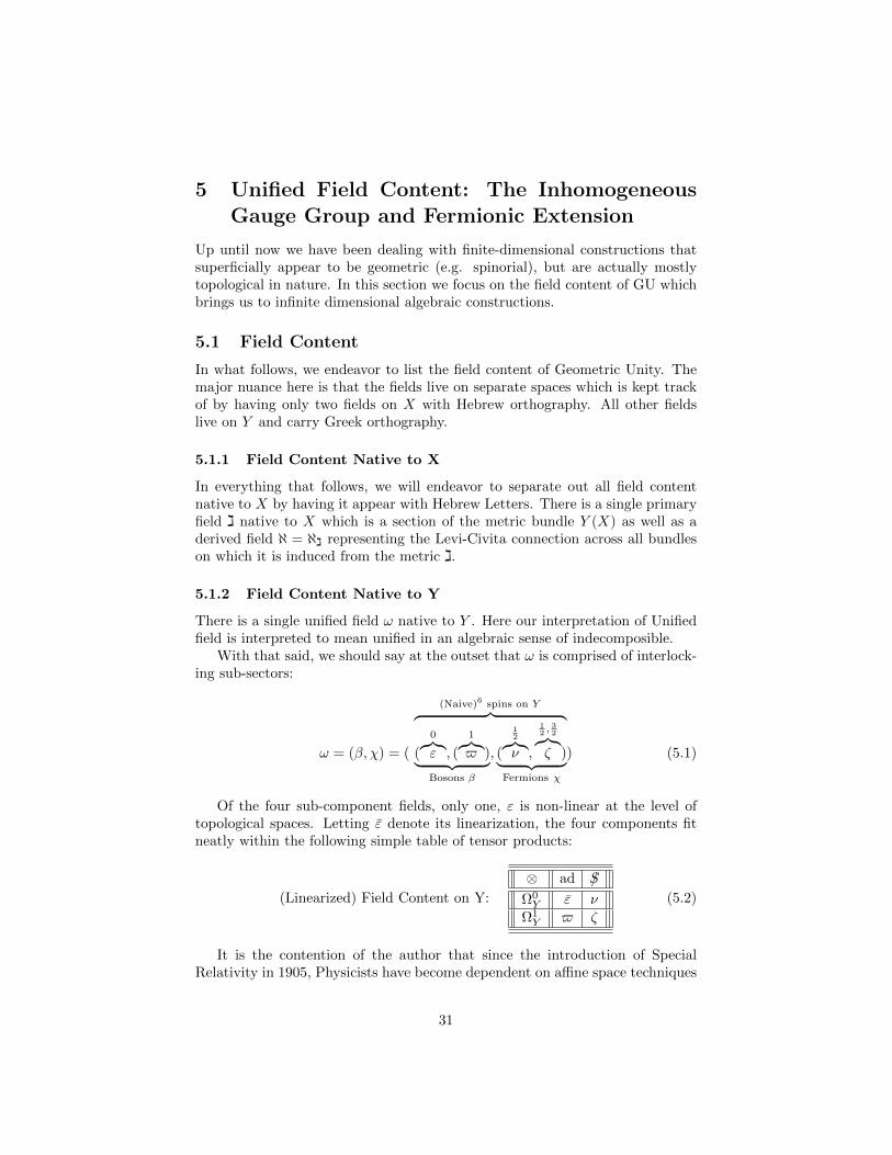
There is a single unified field ω native to Y . Here our interpretation of Unifiedfield is interpreted to mean unified in an algebraic sense of indecomposible.

With that said, we should say at the outset that ω is comprised of interlock-ing sub-sectors:

ω = (β, χ) = (

(Naive)6 spins on Y︷ ︸︸ ︷(

0︷︸︸︷ε , (

1︷︸︸︷$ )︸ ︷︷ ︸

Bosons β

, (

12︷︸︸︷ν ,

12 ,

32︷︸︸︷ζ )︸ ︷︷ ︸

Fermions χ

) (5.1)

Of the four sub-component fields, only one, ε is non-linear at the level oftopological spaces. Letting ε denote its linearization, the four components fitneatly within the following simple table of tensor products:

(Linearized) Field Content on Y:

⊗ ad /S

Ω0Y ε ν

Ω1Y $ ζ

(5.2)

It is the contention of the author that since the introduction of SpecialRelativity in 1905, Physicists have become dependent on affine space techniques

31

for their understanding of relativistic mechanics as well as both classical andquantum field theories. While space-time has obviously not been considered flatsince Einstein and Grossman first introduced General Relativity in 1913, we arerather more sympathetic to the emphasis on affine space than our frequentirritation with excuse making for Minkowski space techniques might suggest.

Simply put, we see affine physics as being central to our understanding of theworld and requiring no excuse making, but believe that the culture has chosenthe wrong affine space and dimensionality for its emphasis given the presenceof gravity.

The simple principle we follow here is that we should implement on theaffine space of connections what we are otherwise tempted to do on flattenedspace-time. To this end we set notation.

5.2 Infinite Dimensional Function Spaces: A,H,N .

The so-called Gauge Group of automorphisms of PH is defined to be:

H = Γ∞(PH ×Ad H) (5.3)

where the space of connections for PH

A = Conn(PH) (5.4)

is an affine space modeled on the right H-module

N = Ω1(Y, ad(PH)) (5.5)

which carries a right action of the group

A×H −→ A (5.6)

so that the affine difference map

δ : A×A −→ N δ(A,B) = A−B ∈ N (5.7)

is an H-equivariant map of right H-spaces.

5.3 Inhomogeneous Gauge Group: GThe reliance on affine Minkowski Space together with its Lorentz and Poincaresymmetry groups is somewhat curious in the presence of General Relativity.Yet given the success of analysis on affine space we are given to speculate thatfundamental physics may in fact be reliant on an affine space as more than anapproximation or pedagogical aid.

The gauge group H can be augmented (in analogy to the Lorentz GroupSL(2,C) to become a subgroup of its own natural inhomogeneous extension.

32

Definition 5.1 The Inhomogeneous Gauge Group G is defined (in analogyto the Poincare group) to be the semi-direct product

G = HnN (5.8)

of the gauge group H with the space of ad-valued one-forms N = Ω1(ad(PH))viewed as a right H-module, so that the explicit group multiplication rule:

g1 · g2 = (ε1, $1) · (ε2, $2) = (ε1 · ε2,Aut(ε−12 , $1) +$2) (5.9)

for all εi ∈ H and $j ∈ N defines the semi-direct product structure.

5.4 Natural Actions of G on A.

Having defined a new group augmenting the usual gauge group, it is worthnoting that the actions of H on the space of connections A extend naturally tothe new group G incorporating the additional inhomogeneous affine translationsN .

5.4.1 Right Action by G on A

This inhomogeneous gauge group G can be seen as acting naturally on the righton the space of gauge potentials or connections A via

A · g = A · (ε,$) = A · ε+$ (5.10)

extending the usual right action A A · ε of an element of the gauge groupε ∈ H on an arbitrary connection A ∈ A.

5.4.2 Left Action by G on A

We also have a left action of G on A via

g ·A = (ε,$) ·A = (A+$) · ε−1 (5.11)

extending the left action A A · ε−1 gotten from the usual right action of Happlied to the inverse element ε−1 ∈ H.

5.5 Fermions and SUSY

Super-symmetry has a curious status within both Mathematics and Physics. Itis both incredibly natural by some measures, as well as being rather artificialby others. It is not a true symmetry, its ‘integrals’ are not real integrals, andits ‘dimensions’ are not true dimensions. Nevertheless, the dictionary betweenBosonic and Fermionic constructions is astounding (at least to us). This isinterpreted by the author as consistent with a signature of a problem whereSuper-symmetry is likely very important but somehow thoroughly misinstanti-ated by its often fanatical proponents compensating for its failure to materializein any physical experiment.

33

If super-symmetry is taken to be natural, then surely so-called super-space isits most natural representation by an action. Here, it seems that affine nature ofGalilean transformations gives us an interpretation for super-symmetric chargesas the square roots of affine translations.

Yet, knowing that Minkowski space is simply an approximation to non-affinespaces is somewhat discouraging if we are to build an entire theory that leansso heavily on flat translations when both non-trivial geometry and topologythreaten to significantly complicate the picture. By contrast, the affine space ofgauge potentials is intrinsically affine in nature no matter what the geometryand topology are on which those potentials live. This is why we find it moreappealing to see Fermionic ν and ζ as potential square roots of the as-if Galileangroup N = Ω1(Y, ad). This is also theoretically appealing as the concept ofelectrons and positrons being some kind of square roots of photons is potentiallyvery appealing given the role of Feynman diagrams in perturbation theory. The

Figure 4: ”Is the Electron a Square Root of a Photon?”

general rubric here is that expressions like (ν · ζ) can be given meaning directlyas elements of N while expressions like ζa · ζb are harder to directly interpret astranslations without more machinery as they do not initially land in the properspace N and would have to be moved in gauge-covariant fashion.

We may return to this in future work but do not wish to say much more asthe subject of modern SUSY is rather delicate given the steadfast failure of itspredicted space-time superpartners to materialize. We note however that thezoo of sleptons, squarks, gluinos and the like are all based on internal symme-try remaining the same and space-time symmetry changing spin. In a theorysuch as GU, there is no internal symmetry. Ergo, the (infinite dimensional)superpartners would not need to have the same internal quantum numbers any-more than they would need to carry the same space-time spins. This asks thequestion: if the universe is GU like rather than Standard-Model like, are thesuperpartners we seek already here and based on an affine space different fromspace-time with no-internal symmetry of which to speak?

5.6 Relationship of the Inhomogeneous Gauge Group toStandard Analysis

A brief digression is in order to relate what we are doing to the standard analysisof gauge potentials under gauge symmetry. To begin with, the usual object

34

of study in quantum field theory is the space of connections modulo gaugeequivalence, or:

A/H (5.12)

in our notation.This is equivalent, at an initially irrelevant level, to the expression

A/H = (H×A)/(H×H) (5.13)

by Cartesian product with a second copy of the gauge group in both numeratorand denominator.

But by the choice of a connection A0 we have A = N as our affine spacenow has an origin while we note that the Semi-direct product of topologicalgroups is set theoretically a product of the underlying spaces if not exactly atthe algebraic level. Thus we have:

A/H = (H×A)/(H×H) = (HnN )/(H×H) = G/(H×H) (5.14)

= (G/H)/H

and our investigations in this area are an analysis of the numerator quotient inthis context.

6 The Distinguished connection A0 and its con-sequences.

All of the preceding is general and did not depend on the choice of any particularconnection. However, besides the ability to contract and project within theEinstein-Riemann paradigm, the secondary benefit we have discussed is theexistence of a distinguished Levi-Civita connection.

It is worth briefly recalling how this connection comes into being by sum-moned from the choice of metric. Let g ∈ Γ2(S2(T ∗)) be a metric on thetangent bundle of a manifold M . Then if β ∈ Ω1(T ∗) is a one form on M andg ∈ Γ2(S2(T )) is the dual metric, then

∇gβ = dβ︸︷︷︸Λ2(T∗M)

⊕ Lgβ(g)︸ ︷︷ ︸S2(T∗M)︸ ︷︷ ︸

T∗M⊗T∗M

∈ Ω1(M,T ∗) (6.1)

or, in other words, the exterior derivative is already half of a connection. Toget the other half, we use the remaining naturally occurring derivative (the Liederivative L(g)) to Lie differentiate a symmetric two tensor. The main trick,however is that the metric is actually used twice, as the Lie derivative requiresa vector field to pick a direction. And since we are operating on a 1-form β. wemust turn it into a vector field using the same metric that is to be differentiated.As such, the Levi-Civita connection is summoned via the Lie derivative’s abilityto complement the exterior derivative and provide its missing half.

35

We now assume, however, that there is a distinguished choice of connectionA0 (such as that which we have just constructed for a given metric), which hasbeen made and can be utilized in what follows. In our case, we begin with ametric ,ג which determines a connection Aleph ℵג on the bundle TX. At thatpoint, the connection ℵ determines a metric gℵ on TY given the metric dataalready present on the horizontal and vertical tangent sub-bundles HY and VY .This, in turn, determines a Levi-Civita connection ∇gℵ = ∇0 which, by abuseof notation, we will consider as determining a spin connection on the structurebundle PH of Dirac spinors over Y . When we have temporarily fixed a givenmetric ג on X giving rise to this spin connection on Y , we will refer to theconnection as A0 ≈ ∇0 ≈ d0 as needed and when the possibility of confusion islikely resolved by context.

As a preliminary note, we remind ourselves that the choice of a distinguished

connection results in a canonical isomorphism AA0∼= N giving us an action of G

on N induced from the right action of G on A. Thus, if a connection A ∈ A isexpressed relative to a base connection A0 as A = A0 + α, we now have a rightaction of G on N which can be expressed via the explicit formula:

α · g = α · (ε,$) = ε−1(α)ε+ ε−1(dA0ε) +$ (6.2)

on the space of connections A.

6.1 The Tilted Map τ into G: the Homomorphism Rule

Lemma 6.1 Given a base connection A0 ∈ A, the map

τA0 : H −→ G (6.3)

given explicitly by

τA0(h) = (h, δ(A0, A0 · h)) = (h,A0 −A0 · h) = (h,−h−1(dA0

h)) (6.4)

is an injective Lie Group homomorphism. 7

Proof: The map is clearly injective because it is the identity map onto andinto the first factor in the semi-direct product. To see that it is a Lie-grouphomomorphism, we argue that:

τA0(h1 · h2) = (h1 · h2,−(h1 · h2)−1(dA0

(h1 · h2))) (6.5)

= (h1 · h2,−((h−12 · h

−11 )((dA0

h1) · h2 + h1 · (dA0h2)))

= (h1 · h2,−(h−12 · (h

−11 (dA0h1)) · h2 + h−1

2 · (dA0h2))

(h1,−h−11 (dA0h1)) · (h2,−h−1

2 (dA0h2)) = τA0(h1) · τA0(h2)

7There appears to have been multiple sign conventions and some notational shifts withinthe files from which this section was reassembled. We will endeavor to sort this out but theremay be 2 or more conflicting convetions in this section.

36

QED.

This subgroup τA0(H) ⊂ G is important to our constructions and thus war-

rants a name to distinguish it from the more obvious H subgroup.

Definition 6.2 The image of H inside G under τA0 will be referred to as theThe Tedha8 Gauge Group HτA0

inside G, with the image of H simply in-cluded onto the first factor of G and sent to 0 in the second factor being referredto as the Trivial or Seedhe Gauge Group to avoid confusion.

6.2 Stabilizer Subgroup

If we act on the space of connections using the natural right action of theinhomogeneous gauge group G we may ask what the stabilizer subgroup is forthe Levi-Civita spin connection A0. To this end, solving for g ∈ G stabilizingA0 we have:

0 = A0 · g −A0 = A0 · ε+$ −A0 = (A0 + ε−1 · d0ε+$)−A0 (6.6)

implying$ = −ε−1dA0

ε (6.7)

so that the flipped τ map:τ0 : H −→ G (6.8)

given by:τ0(h) = (h,−h−1d0h) (6.9)

provides a parameterization.

6.3 G as Principal bundle: Action by Tilted Gauge Trans-formations Rule

The choice of a base connection A0 determines a surjection

πA0 : G −→ N (6.10)

given byπA0

(g) = πA0((ε,$)) = ε$ε−1 + (dA0

ε)ε−1 (6.11)

which can be taken to be the projection map in the homogeneous principalH-fibration:

H → PH = G↓ πA0

B = G/HτA0= N

(6.12)

determined by the right action of H as tilted subgroup on G

g · τA0(h) = (ε,$) · τA0

(h) = (ε · h, h−1$h− h−1(dA0h)) (6.13)

via the τA0homomorphism.

8This is transliterated Hindi for slanted or crooked and got stuck in the author’s headmany years ago via his wife’s usage. Seedhe means straight by the same token.

37

Lemma 6.3 The map πA0 , is the projection map for the natural right actionof τA0(H) on G.

Proof:

πA0(g ·τA0

(h)) = πA0((ε,$) ·(h,−h−1dA0

h)) = πA0((ε ·h, h−1 ·$ ·h−h−1dA0

h))(6.14)

= (ε · h)(h−1$h− h−1dA)h)(ε · h)−1 + (dA0(ε · h))(ε · h)−1

= (ε·h·h−1$h·h−1·ε−1−ε·h·h−1dA)h)·h−1·ε−1+((dA0

ε)·h))·h−1·ε−1+(ε·dA0(h)))·h−1·ε−1

= ε ·$ · ε−1 − ε · (dA)h) · h−1 · ε−1 + (dA0

ε) · ε−1 + ε · (dA0h) · h−1 · ε−1

= ε ·$ · ε−1 + (dA0ε) · ε−1 = πA0((ε,$)) = πA0(g)

As a benefit of this homogeneous principal fibration, we also gain a left actionof G on B = N via

Lemma 6.4 The rule

g · γ = (ε,$) · γ = ε($ + γ)ε−1 + (dA0ε)ε−1 (6.15)

determines a left group action of G on N .

Proof: The lemma can be seen from direct application of the preceding discus-sion and rules:

(g1 · g2) · γ = ((ε1, $1) · (ε2, $2)) · γ = (ε1 · ε2,Aut(ε−12 , $1) +$2) · γ (6.16)

+(ε1 · ε2)(Aut(ε−12 , $1) +$2 + γ)(ε1 · ε2)−1 + (dA0

(ε1 · ε2))(ε1 · ε2)−1

= ε1 ·ε2 · ((ε−12 ·$1 ·ε2)+$2 +γ) ·ε−1

2 ·ε−11 +((dA0

ε1) ·ε2 +ε1 · (dA0ε2)) ·ε−1

2 ·ε−11

= ((ε1·$1·ε−11 )+ε1·(ε2·$2·ε−1

2 )·ε−11 +ε1·(ε2·γ·ε−1

2 )·ε−11 −(dA0

ε1)·ε−11 −ε1·((dA0

ε2)·ε−12 )·ε−1

1

= ε1 · (ε2 · ($2 + γ) · ε−12 + (dA0

ε2) · ε−12 +$1) · ε−1

1 + (dA0ε1) · ε−11

= (ε1, $1) · ((ε2, $2) · γ) = g1 · (g2 · γ)

6.4 Map out of G to spaces of connection: Gauge Equiv-ariance

Lemma 6.5 The choice of a base connection A0 also determines a map

µA0 : G −→ A×A (6.17)

into the space of “bi-connections” A×A according to:

µA0(g) = µA0

((ε, $)) = (A0 +$, A0 · ε) ∈ A×A (6.18)

= (A0 +$, A0 + ε−1(dA0ε)) (6.19)

so that the map µA0 of right H spaces is HτA0-equivariant.

38

Proof: The proof is immediate according to the following:

µA0(g · τA0

(h)) = µA0((ε, $) · τA0

(h)) = µA0((ε, $) · (h,−h−1dA0

h)) (6.20)

= (dA0+ h−1$h+ h−1(dA0

h), dA0+ h−1(ε−1(dA0

ε))h+ h−1(dA0h)) ∈ A×A

= (A0 +$,A0 + ε−1(dA0ε)) · h = µA0(g) · h

QED

Definition 6.6 The map µA0will be called the Bi-Connection map in what

follows.If we use the natural action of HτA0

on A to form an associated bundle ofaffine spaces with total space TA, the bi-connection can be seen as determiningtwo natural sections σ1, σ2 depicted below as:

A → TAπ ↓↑ σ1,2

B(6.21)

The values of these two sections σ1,2 will be known as the A and B connectionsrespectively, written as

Aω = ∇0 +$ω Bω = ∇0 + ε−1ω (∇0εω) (6.22)

when needed separately.

7 The Augmented or Displaced Torsion

The Torsion Tensor has always presented a puzzle. It is traditionally introducedvery early on in the study of Riemannian geometry and is almost never heardfrom thereafter except in niche explorations. One modern interpretation of thisstylized fact could be that the torsion of a connection is afflicted with a diseasethat keeps it from being ‘gauge covariant’ and thus useful to the mainstream ofmodern theory.

An important principal of some potential relevance here is seldom statedexplicitly. It is that when faced with a mathematical disease, it is often advan-tageous to seek a second disease in the hopes that an even number of diseasesmight be poised to kill each other in pairs.

7.1 Augmented Torsion and its Transformations

Our strategy is to think as follows. There are effectively two different ways oftransforming a connection. One is by gauge transformation and the second is by‘translation’ by adding to it an ad-valued 1-form on Y . Because these two groupactions have been intertwined within the inhomogeneous gauge group, there areeffectively two separate ways to transform the spin connection inherited fromthe Levi-Civita connection of the metric. Taking their difference is meaningfulbecause both transformed connections carry exactly the same global disease

39

that renders them non-gauge covariant. Therefore the ability to generate twoseparate connections with a common disease from a single group element in Gwhich is still a set theoretic if not algebraic product is meaningful.

Definition 7.1 There is a well defined map from the inhomogeneous gaugegroup G to the space of generalized torsion tensors N viewed as a right H-module, given by:

δ µA0: G −→ N (7.1)

so that we can define The Augmented Torsion Tensor Tg = Tε,$ = T ((ε,$))according to

Tg = δ(µA0((ε,$))) (7.2)

which is given explicitly by:

Tg = $ − ε−1(dA0ε). (7.3)

The Augmented Torsion is distinguished in that it is very well behaved underHτA0

transformations. This can be seen explicitly as:

Lemma 7.2 The augmented torsion tensor as a map from G to N is equivariantas a map of right HτA0

-spaces.

Proof:Tg·τA0

(h) = T(ε,$)·τA0(h) = T(ε·h,h−1$h−h−1(dA0

h)) (7.4)

= h−1$h+ h−1(dA0h)− (ε · h)−1(dA0(ε · h))

= h−1$h+ h−1(dA0h)− (h−1 · ε−1)((dA0

ε) · h+ h−1 · (dA0h))

= h−1($ − ε−1(dA0ε))h = Ad(h−1, Tg)

QEDIn essence, the group G is topologically the Cartesian product of two separate

groups acting on the common space A. The presence of a single connection ∇0

and a single element β = (εβ , $β) ∈ G leads to two separate new connectionsA = (∇0) · ε,B = (∇0) ·$ which in an affine space suggests taking a differenceA−B ∈ N which diagrammatically appears as

Aε

∇0 × N$

A

(7.5)

7.2 Summary of spaces and maps

The following diagram summarizes much of what we have just discussed:

HτA0→ G

µA0−→ A×A δ−→ NHR↓ πA0

AA0∼= NGL

(7.6)

with respect to the integral spin fields. The addition of the half-integral spinfields leads to a sort of super-space like version of the above.

40

8 The Family of Shiab Operators

With this machinery notated and established, we can turn to the second majoradvantage of working in the Meta-Riemannian paradigm.

Figure 5: Ship In a Bottle Construction.

In essence, gauge theory and relativity have been disconnected because ofthe incompatibility of contraction and gauge covariance of terms within theaction. The former typically contracts between a differential form and someother bundle associated to the tangent bundle where the differential form isvalued, while gauge rotation typically acts on the latter bundle without touchingthe forms.

The ‘Ship in a Bottle’ construction attempts to get around this difficulty. Byincorporating the gauge group into the contraction operator, the gauge grouprotates only the bundle valued portion of a collection contracting forms Φiin which these special invariant differential forms are valued in such a way thatit exactly compensates for the a symmetry of treatment in the form being con-tracted. Suppose for example that η is a gauge covariant ad−valued differentialform. Then a Shiab contraction operator might look like:

· εη = ∗ni1±1

2 [(ε−1Φrε) ∧ ∗mη]± (8.1)

or perhaps a sum of such terms, where typically Φr is a normed Lie AlgebraValued r-form valued in an invariant subspace of the structure group of thetangent bundle and the bracket is either a commutator or an anti-commutatorwith a factor of i out front in the case of the latter.

There is most likely a byzantine taxonomy of such objects along the linesof what Reese Harvey detailed for the Clifford Algebras in his book on Spinorsand Calibrations.

The author is no longer in a position to go chasing after the complete pictureand simply details some of the available tools for customizing such operators.

8.1 Pure Trace Elements

As vector spaces over the real numbers,

Λ∗(T ∗X) = Cl(T ∗X) (8.2)

41

but where the algebraic structures are somewhat different. In our case, when Yinherits a (7, 7) metric, we have an equivalence at the level of vector spaces:

ϑ : Λ∗(T ∗Y ) −→ Cl(T ∗X) = R(128). (8.3)

If ClR(T ∗Y ) is included in its own own complexification it can be seen withinthe matrix algebras

spin(64, 64) −→ u(64, 64)↓ ↓

ϑ : gl(128,R) −→ gl(128,C)| | | |

ϑ : ClR(T ∗Y ) −→ ClC(T ∗Y )

(8.4)

which commute on:

so(64, 64) “ = ” (Λ2 ⊕ Λ6 ⊕ Λ10 ⊕ Λ14)︸ ︷︷ ︸/SL⊗/SR=/SL⊗/S

∗L=/S∗R⊗/SR

⊕ (Λ1 ⊕ Λ5 ⊕ Λ9 ⊕ Λ13)︸ ︷︷ ︸Λ2(/SL)⊕Λ2(/SR)

⊂ ClR(7,7).

(8.5)What differs instead is what happens on

u(64, 64)/so(64, 64) “ = ” k0Λ0⊕ k3Λ3⊕ k4Λ4⊕ k7Λ7⊕ k8Λ8⊕ k11Λ11⊕ k12Λ12

(8.6)which must be multiplied by various factors of i inside the complexification.

Definition 8.1 Let Φi14i=0 be a basis for the invariant subspaces of

[Λi(R7,7)⊗ u(64, 64)]Spin(7,7) (8.7)

seen as a Spin(7, 7) representation.

8.2 Thoughts on Operator Choice

The particulars of the Shiab operators are workmanlike and not of much interest.The interesting aspect of them, is that they all essentially look like contractingover indices in the fashion familiar from Riemannian tensor geometry, but withsome aspect of conjugation by the gauge group element ε ∈ H ⊂ G living insidethe inhomogeneous gauge group G as a non-linear sigma-field of sorts.

The author remembers choosing them years ago via representation theorytechniques involving highest weight representations rather than by the moreindicial methods presented here with invariant elements Φi. The advantage wasthat the Bianchi identity was able to pick the best and most appropriate operatorin different circumstances. Unfortunately, the author is no longer conversant inthat language and has been unable to locate the notes from decades ago thatoriginally picked out the operator of choice to play the role of the Swerve here· . The author either hopes to find the original calculations or to get back tothe point where he can reconstruct this argument based on using the Bianchiidentity to guarantee gauge perpendicularity and/or use the Bianchi identity toguarantee automatic solution of a differential equation in the curvature.

Note: A brief discussion of additional tools for Shiab construction has beenmoved to a a short technical appendix.

42

9 Lagrangians

There are multiple considerations in putting forward Lagrangians in this con-text. In particular there are issues of redundant equations, Bianchi Identi-ties, cohomological considerations for deformation complexes, so-called Super-symmetry, agreement with prior physical equations, and the issue of Dirac-Pairs where one set of more restrictive (usually first order) equations guaran-tees the solution of the equations of a different related (usually second order)Lagrangians.

9

9.1 The 1st Order Bosonic Sector

The purely Bosonic portion of the action is a real valued function:

IB1 : G ×MET (X1,3) :−→ R (9.1)

While there are other possibilities to explore for the choice of the Shiaboperator, Let

· ε : Ω2(Y 7,7, ad) −→ Ωd−1(Y 7,7, ad) (9.2)

we will begin with one10 which makes the parallel to Einstein’s contraction ofthe full Riemannian curvature explicit:

· εξ = [(ε−1Φ1ε) ∧ (∗ξ)]︸ ︷︷ ︸Ricci Like

−∗2

[(ε−1Φ1ε)︸ ︷︷ ︸gµν - like.

∧ ∗ [(ε−1Φ2ε) ∧ (∗ξ)]]︸ ︷︷ ︸Ricci Scalar Like

(9.3)

for a gauge covariant ad-valued 2-form ξ ∈ Ω2(Y, ad).Here, as in Einstein’s case, the Weyl curvature tensor is annihilated by the

contraction operator above so the operator preserves and mixes only the ana-logues of the Ricci and Scalar curvature components.

The puzzle of how to kill off the Weyl curvature contribution to recoverRiemannian geometry’s ability to form Einstein tensors for gravity in such away as to preserve Ehresmannian gauge covariance is part of what is meant byGeometric Unity. This leads to a model that abstracts the Einstein-Hilbert andChern-Simons actions to generate linear field equations in the Riemannian and

9We have closely followed the history referred to by Dirac in his 1963 Scientific AmericanArticle discussing Schrodinger and the Multiple iterations of Einstein’s (and Grossman’s)introduction of General Relativity and taken from them that an author will have to fine tunethe instantiation of a new idea. What we take away from this is that the tiny minority ofauthors who put forward new physical law have to have the right to explore instantiations ofnew ideas without the community over indexing on the instance put forward. As with anyrelease, the interested community is welcome to send bug fixes.

10The author used to construct such objects from representation theory concepts like highestweights. The Shiab operator that he settled on (but cannot yet now locate) was chosen for itsproperties relative to the Bianchi identity. Even if it can be located, it will be in a differentlanguage with which the author no longer feels entirely familiar. So it is.

43

Ehresmannian curvature tensors via an action IB1 which for only the Bosonic

fields of integral spin (ε,$ on Y and ג on X) looks like:

IB1 (ωY , (Xג = IB

1 ((εY , $Y ), (Xג (9.4)

=<

Shifted

Torsion︷︸︸︷Tω , ∗︸︷︷︸

Hodge

Star

(

Einstein

Ricci

Shiab︷︸︸︷· ω ( FBω︸︷︷︸

Metric

Curvature

+

C-S Like Terms︷ ︸︸ ︷1

2dBωTω +

1

3[Tω, Tω])+

κ1

2Tω︸︷︷︸

Shifted

Torsion

) >

Zorro

Metric︷︸︸︷g

ג

=

∫Y

Tr(($−ε−1d0ε)∧∗([(ε−1Φ1ε) ∧ (∗(·))]︸ ︷︷ ︸Ricci Like

−∗2

[(ε−1Φ1ε)∧∗ [(ε−1Φ2ε) ∧ (∗(·))]]︸ ︷︷ ︸Ricci Scalar Like

)

(ε−1Rθijσε+1

2(d0 + ε−1d0ε)($ − ε−1d0ε) +

1

3[$ − ε−1d0ε,$ − ε−1d0ε]))

+κ1

∫Y

Tr(($ − ε−1d0ε) ∧ ∗($ − ε−1d0ε))

where:

1. Rθijσ is the Spinor bundle’s Riemannian curvature induced from the Levi-Civita connection.

2. Tω = $ − ε−1d0ε ∈ Ω1(Y, ad) is the augmented torsion tensor.

3. The Shiab Operator · ω on an ad-valued 2-form ξ ∈ Ω2(Y, ad)is given inaccordance with the Einsteinian contraction

· εξ = [(ε−1Φ1ε) ∧ (∗ξ)]︸ ︷︷ ︸Ricci Like

−∗2

[(ε−1Φ1ε) ∧ ∗ [(ε−1Φ2ε) ∧ (∗ξ)]]︸ ︷︷ ︸Ricci Scalar Like

4. The Bω connection is the gauge rotation of the Levi-Civita Spin Connec-tion: Bω = ∇0 + ε−1d0ε

By the calculus of variations we obtain Euler-Lagrange Equations of theform:

dIB1 ,ג) ω)|Y 14 =

Υω

⊕Ξω

∈ Ωd−1(ad)⊕

Ωd(ad)(9.5)

where generallyΞ = DωΥω (9.6)

for some operator differential Dω so that the vanishing of Ξω = 0 need not beconsidered if Υω = 0 by the redundant nature of the second equation.

44

And by gathering up terms we can express them in a fashion that is closerto the more familiar equations of General Relativity. Thus we have:

∂IB1 ((εY , $Y + sα), (Xג

∂s=< α,· ωFAω + ∗κ1Tω >=< α,ΥB

ω > (9.7)

·Fω︸︷︷︸Swerved Curvature= Swervature = Sω

= − ∗ κ1 Tω︸︷︷︸Displaced Torsion︸ ︷︷ ︸

Displasion=Tω

(9.8)

So that if one wanted to locate and recover from a GU equation:

Υω = Sω − Tω = 0 (9.9)

the more familiar terms of the Einstein Field Equations for Gravity, it wouldgenerate an annotated equation along the lines of:

Sω︸︷︷︸Rµν− s2 gµν

= Tω︸︷︷︸Λgµν︸ ︷︷ ︸

Tµν

(9.10)

9.2 Second Order Euler-Lagrange Equations

One of the Claims of Geometric Unity is that we have been unsuccessful inUnifying the four basic equations for Gravity, Non-Gravitational force, Matterand Higgs phenomena because they belong to a Dirac Pair. That is, we believethat the Einstein and Dirac equations belong to a unifying equation which isin the sense of Dirac something of a square root of a different equation orLagrangian related to the Yang-Mills-Maxwell equation and the Higgs versionof the Klein-Gordon equation. Thus we should seek to unifying our equationsand Lagrangians much the way Dirac unified first and second order equationswith his masterstroke To this end we focus on second Lagrangian of 2nd order:

IB2 ((εY , $Y ), (Xג = ||ΥB

ω ||2 (9.11)

∂IB2 ((εY , $Y + sα), (Xג

∂s=< α, 2(d∗Aω·

∗ω + κ1Id)ΥB

ω ) > (9.12)

= 2 < α, d∗Aω·∗ω· ωFAω︸ ︷︷ ︸

New ‘Yang-Mills’ Term

+κ1d∗Aω·

∗ωTω + κ1 ∗· ωFAω + κ2

1Tω > (9.13)

yieldingD∗ωFAω = JBω︸ ︷︷ ︸

Yang-Mills-Maxwell like equation with Bosonic source.

(9.14)

but more efficiently asD∗ωΥω = 0 (9.15)

which is more natural within Geometric Unity.

45

9.3 The Fermionic Sector

In the case of the Fermionic content we can at the classical level take fieldsν, ζ, ν, ζ on Y to be four distinct fields when ultimately we will wish to integrateout the Dirac like operator to take a Berezinian ‘integral’ in the quantum theory.

For ν, ν ∈ Ω0(Y, /S) and ζ, ζ ∈ Ω1(Y, /S) we can begin with operators like:

(ζ− ζ+ ν− ν+

)ρ(ε)·

∗·$++ ∗· (d0 +$+−) $++ d0 +$+−

∗· (d0 +$−+) ∗·$−− d0 +$−+ $−−−$∗++ −d∗0 − $∗+− 0 0

−d∗0 − $∗−+ −$∗−− 0 0

︸ ︷︷ ︸

/Dω

·

ζ+ζ−ν+

ν−

ρ(ε−1)

(9.16)noting that other versions of the theory exist including one with a non-trivialmap in the lower right quadrant of the operator. This two can be made to lookcloser to the Dirac Theory of Spinorial Fermions:

/DFω

(ζν

)ρ(ε−1)

= /Dωχε−1 = 0 (9.17)

where χ contains three generations of observed Fermions as well as Looking-Glass matter, dark Spinorial Matter, Rarita-Schwinger matter and more whileD subsumes the Dirac Operators, and the various subfields of ω accomodate thefunctionings of the CKM matrix, the Higgs-Like soft mass fields, the Yukawacouplings, Gauge Potentials and the like.

Let us compile the Bosonic and Fermionic variations of the Spinorial La-grangian terms in a single term:

ΥF = ∗

dAων + ∗· dAωζ

⊕d∗Aωζ⊕

νζ + ζν +· ζζ

(9.18)

as a kind of 1-form on some SuperSpace-like structure over A:

ΥFω ∈

Ωd−1(Y, /S)⊕

Ωd(Y, /S)⊕

Ωd−1(Y, ad)

(9.19)

which can be combined with the variation of either a first or second order purelyBosonic Lagrangian so as to form:

Υω = ΥBω + ΥF

ω = 0 or Dω∗ΥBω = ΥF

ω (9.20)

At this point, we wish to take this mixed spinorial-tensorial Υω and ask whetherwe are attempting to penalize this expression in our extremization because it is

46

actually the obstruction term for a cohomology theory. That is, we choose toview ‘wedging’ with Υω as the application of a zeroth order operator and askif it possesses a non-trivial square root the in form of a first order differentialoperator δω so that:

Υω = 0 and√

Υω = δω (δω)2 = 0 Cohomology (9.21)

to get a Lagrangian Cohomology theory of at least two steps:

Υω = (δω)2 = δω2 δω1 = 0 (9.22)

of a geometrically meaningful cohomology complex.

10 Deformation Complex

The expected way to have our field equations arise naturally as the obstructionto a cohomology theory, is to first ask about the moduli space of solutions tothe equations. That is, if ω∗ represents a solution to the equations of motionwith Υω∗ = 0, in what are essentially different directions, may we perturb ω∗

to obtain new solutions? To that end we begin first with the purely Bosonicfields on Y and linearize our Tedhe action of the gauge group H on the groupG = H n N via the τ0 homomorphism by linearizing both the groups and theexponential map of the action:

δω1︷︸︸︷ δω2︷︸︸︷Ω1(ad) −→ Ωd−1(ad) −→ 0

⊕ 0 −→ Ω0(ad)︸ ︷︷ ︸

Symmetries:

TeH

−→ Ω0(ad)︸ ︷︷ ︸Fields:

TωG

︸ ︷︷ ︸Equations:

T ∗ωGd−1

(10.1)

——In a certain sense, one can view the usual (twisted) DeRahm complex as the

square root of the of the curvature as dA dAφ = [FA ∧ φ]. The same is truefor the Υ-Spinor-Tensor so we may ask if there is a complex with a co-chainoperator such that: √

Υω = δω (10.2)

where the individual operators are configured so that:

δω1 : Ω0(ad) −→Ω1(ad)⊕

Ω0(ad)δω2 :

Ω1(ad)⊕

Ω0(ad)−→ Ωd−1(ad) (10.3)

and in fact this will give our assemblage11 the structure of a (Bosonic) defor-mation complex.

11Many years ago, while thinking about this, the author passed through Iceland and wasamused to find that a ‘Thing’ in Icelandic was a ‘Governing Assembly’ and as such took toreferring to this governing assemblage for deformations as a Thing with operators Things 1and 2.

47

To expand the concept from purely integral spin fields to include those offractional spin, we are led to linearize equations of the form:

χ =

(ζν

)(10.4)

δω2 δω1 = Υω =

(/Dωχ

· ωFAω + ∗kTω + σ(· ω,Ψ, Ψ)

)= 0 (10.5)

The first step then for us is to examine what we mean by ‘essentially differentdirections’ of perturbation as regards the symmetry built into the problem. Aswe have endeavored to keep our metric theory gauge theoretic, let us first try toremove the uninteresting redundancy that is merely due to the gauge symmetryof the H action.

The effect of an infinitesimal gauge transformation γ ∈ TeH on a pointg = (ε,$) ∈ G = PH is given by:

d

dsg · τA0

(exp(sγ)) =d

ds(ε,$) · τA0

(exp(sγ)) (10.6)

=d

ds((ε,$) · (exp(sγ), exp(sγ)−1dA0

exp(sγ)))

= (DLεγ, dA0γ − [γ,$]) = (DLεγ, dA$γ)

so that we have:

δω1 =

δω1,a⊕δω1,b

=

dAω⊕

DLεω

(10.7)

As for the second operator, we can search for it in the linearization of theequations of motion. To this end we posit:

δω2 =(δω2,a ⊕ δω2,b

)(10.8)

δω2,a = · ω dAω (·) + κ1 ∗ (·) (10.9)

δω2,b = FAω ∧· (·)− κ1 ∗ dBω (·)

Putting this Bosonic piece together with the Spinor deformations gives a dia-

48

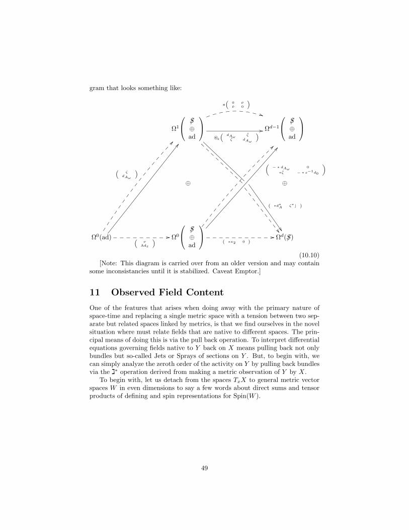
gram that looks something like:

Ω1

/S⊕ad

( ∗d∗A ζ∗c )

∗(

0 νν 0

)))

· ε(

dAωζ

ζ dAω

) // Ωd−1

/S⊕ad

⊕ ⊕

Ω0(ad)

(ζ

dAω

)

@@ BB

(ν

Adε

) // Ω0

/S⊕ad

(− ∗ dAω 0

∗ζ − ∗ ε−1d0

)>> AA

( ∗κ2 0 )// Ωd(/S)

(10.10)[Note: This diagram is carried over from an older version and may contain

some inconsistancies until it is stabilized. Caveat Emptor.]

11 Observed Field Content

One of the features that arises when doing away with the primary nature ofspace-time and replacing a single metric space with a tension between two sep-arate but related spaces linked by metrics, is that we find ourselves in the novelsituation where must relate fields that are native to different spaces. The prin-cipal means of doing this is via the pull back operation. To interpret differentialequations governing fields native to Y back on X means pulling back not onlybundles but so-called Jets or Sprays of sections on Y . But, to begin with, wecan simply analyze the zeroth order of the activity on Y by pulling back bundlesvia the ∗ג operation derived from making a metric observation of Y by X.

To begin with, let us detach from the spaces TxX to general metric vectorspaces W in even dimensions to say a few words about direct sums and tensorproducts of defining and spin representations for Spin(W ).

49

11.1 Fermionic Quantum Numbers as Reply to Rabi’s ques-tion.

To begin with, there is a simple rule for tensor products of defining representa-tions and spinors whereby the tensor product

W ⊗ /SW = /SW ⊕ /RW (11.1)

breaks into a piece representing the action of gamma matrices as spinor en-domorphisms and a second piece giving the pure Rarita-Schwinger spin 3/2representation corresponding to the sum of the highest weights of the factors.

We note further, that spinor representations carry the property of the ex-ponential in that they take in direct sums as input and return products of thespinors of the summands as output.

W = U ⊕ V /S(W ) = /S(U ⊕ V ) = /S(U)⊗ /S(V ) (11.2)

Both of these are likely to be well known to physicists. Some what lessfamiliar is that the Rarita-Schwinger representation has slightly odd behaviorwhen applied to direct sums of vector spaces.

The rule here is that

/R(W ) = /R(U ⊕ V ) =

/R(U)⊗ /S(V )

⊕/S(U)⊗ /R(V )

⊕/S(U)⊗ /S(V )

(11.3)

with an odd re-appearance of a final term which has purely spinorial with no3/2 spin Rarita-Schwinger component.

To apply the above to our situation we recognize that ζ represents a spinorvalued 1-form and ν a spinor on Y with U representing the Horizontal and Vthe Vertical normal bundle Nג to the metric as an embedding

ג : X −→ Y. (11.4)

Even at zero-level before the introduction of higher Jets, the pull back ofν, ζ and their host bundles is potentially of considerable interest.

11.2 The Three Family Problem in GU and Imposter Gen-erations.

‘Who ordered that?’ -Isidore Rabi on the Muon

We have had to restrict ourselves to a world without auxiliary internal quan-tum numbers as essentially everything has been generated endogenously fromX4. This leaves the question of why we appear to see a rich offering of repeatinginternal Fermionic quantum numbers.

50

In fact we will make two likely to be controversial claims in this section thatmay appear to fly in the face of experimental observation. The first is that we donot believe that nature has simply repeated herself three times albeit at differentmass scales. While we do believe that a second copy of Fermionic matter matchesthis description, we believe that a third family is merely effectively identical tothe other two and, presumably, only at low energy.

Secondly, while we are often told that the discovery of parity violation inbeta decay found in the 1950s by Chien-Shiung Wu following theories of Yangand Lee, proves that nature is intrinsically chiral, we will again hazard the guessthat it is merely effectively chiral so that at a deeper level it remains intrinsicallybalanced between left and right. To see this more clearly we will decomposeour Fermionic sector under the decompositions of S(T/)∗ג ∗Y )) and R(T/)∗ג ∗Y ))under

T)∗ג ∗Y ) = T ∗X ⊕Nג (11.5)

To this, our rolled up Fermionic complex looks quite different under theabove tangent space decomposition:

Z−1

2

⊕Q+

32

−−⊕−−F−1

2

Spin(7,7)+

832−

⊕(F−1

2

)Spin(7,7)+

64−

Ω1(/S−,Y14)

ζ−

−→

Z+

12

⊕Q−3

2

−−⊕−−F+

12

Spin(7,7)+

832+

⊕(F+

12

)Spin(7,7)+

64+

Ω13(/S+,Y14)

⊕ ⊕

( (

F−12

)Spin(7,7)+

64−

)Ω0(/S+,Y14)

ν+

((F+

12

)Spin(7,7)+

64+

)Ω14(/S−,Y14)

0 −− −−−−−−⊕−−−−−− −− −−−−⊕−−−− −− 0

( (

F+12

)Spin(7,7)−

64+

)Ω0(/S−,Y14)

ν−

( (F−1

2

)Spin(7,7)−

64−

)Ω14(/S+,Y14)

⊕ ⊕

(F+

12

)Spin(7,7)−

64+

⊕F+

12

⊕Q−3

2

⊕Z+

12

Spin(7,7)−

832+

Ω1(/S+,Y14)

ζ+

−→

(F−1

2

)Spin(7,7)−

64−

⊕F−1

2

⊕Q+

32

⊕Z−1

2

Spin(7,7)−

832−

Ω13(/S−,Y14)

51

where we have used the notation:

F±12

=

2∓ ⊗ 16+

⊕2± ⊗ 16−

Q±32

=

6∓ ⊗ 16+

⊕6± ⊗ 16−

Z±12

=

2∓ ⊗ 144+

⊕2± ⊗ 144−

(11.6)

for Spin(1, 3)×Spin(6, 4). The idea being explored here is that the full operatordepicted decouples effectively into two separate Dirac like operators, when thereis no vacuum expectation value pulling the various sub-fields of $ to valuessignificantly above zero. Thus we assert that a non-chiral total theory splitsat the emergent level into two separate chiral theories and that the one abovethe dashed line corresponds to matter in our world with the other sectors notlabeled by F to the left and above the line are currently dark to us.

11.3 Explict Values: Predicting the Rest of Rabi’s Order.

With all that said above, we can now predict what the internal quantum num-bers will likely be if GU is correct as per the following:

Names Multiplicity Dimension Structure Notation Name(s)

Left Quarks 1 6 [3× 2]n=1L

Left Anti-Quarks 1 3 [3× 1]n=2L

Left Anti-Quarks 1 3 [3× 1]n=−4L

Left Leptons 1 2 [1× 2]n=−3L

Left Anti-Lepton 1 1 [1× 1]n=6L

Left Anti-Lepton 1 1 [1× 1]n=0L

after reductions of the structure groups. A more violent regime would be ex-pected to reveal differences that are more profound than mere mass discrepan-cies.

Another surprise would be a new cousin spin- 32 ‘generation’ Q+

32

, in which

the logic of the known matters is reversed in the sense that it is right handedmatter and left handed anti-matter that feel the effects of Weak-Isospin.

Names Multiplicity Dimension Structure Notation Name(s)

1 6 [3× 2]n=−1L

1 3 [3× 1]n=−2L

1 3 [3× 1]n=+4L

1 2 [1× 2]n=+3L

1 1 [1× 1]n=−6L

1 1 [1× 1]n=0L

52

Number Multiplicity Dimension Structure Electric Charge Name(s)

1 1 16 [8× 2]n=−3L −1, 0

2 1 8 [8× 1]n=0L 0

3 1 8 [8× 1]n=6L 1

6 1 12 [6× 2]n=1L + 2

3 ,−13

5 1 6 [6× 1]n=2L + 1

3

4 1 6 [6× 1]n=−4L − 2

3

12 1 9 [3× 3]n=2L + 4

3 ,+13 ,−

23

11 1 9 [3× 3]n=−4L + 1

3 ,−23 ,−

53

8 1 6 [3× 2]n=7L + 5

3 ,+23

7 1 6 [3× 2]n=−5L − 1

3 ,−43

20 *1 6 [3× 2]n=1L + 2

3 ,−13

13 1 6 [3× 2]n=5L + 4

3 ,+13

10 1 3 [3× 1]n=−2L − 1

3

9 1 3 [3× 1]n=−8L − 4

3

20 *2 6 [3× 2]n=1L + 2

3 ,−13 Imposter Quarks

18 2 3 [3× 1]n=2L + 1

3 Imposter Anti-Quarks

19 2 3 [3× 1]n=−4L − 2

3 Imposter Anti-Quarks

15 1 3 [1× 3]n=6L +2,+1, 0

16 1 2 [1× 2]n=−9L −2,−1

23 1 1 [1× 1]n=0L 0 Imposter Anti-Neutrino

14 1 3 [1× 3]n=0L +1, 0,−1

21 *1 2 [1× 2]n=−3L −1, 0 Imposter Leptons

22 1 1 [1× 1]n=6L +1 Imposter Anti-Electron

17 1 2 [1× 2]n=3L +1, 0

21 *1 2 [1× 2]n=−3L −1, 0

11.4 Bosonic Decompositions

As we have argued previously, the observed standard model appears to be con-sistent with a reduction of structure group of the full Dirac Spinors on Y inthree stages

1. First: to a splitting of T ∗Y to T ∗X together with the normal bundle Nגof the metric seen as an embedding, according to T)∗ג ∗Y ) = T ∗X ⊕Nג.

2. Second to a Maximal Compact Subgroup of structure group of the Normalbundle Nג from Spin(6, 4) to Spin(6)× Spin(4) ∼= SU(4)× SU(2)× SU(2)in accordance with the Pati-Salam theory.

3. Lastly to a complex structure on the Normal bundle from Spin(6)×Spin(4)to U(3) × U(2) where a final reductive factor may be removed or not byprivileging a complex volume form.

53

As far as understanding the picture of the force carrying gauge potentials, weare really looking to understand what parts of Ω1(Y, ad) carries meaning for usalready within the standard model. To that end we can see that at the levelof vector spaces if not as algebras, the ad−bundle is equivalent to the exteriorbundle on Y . Both the branching of the 1-forms Ω1(Y ) and the ad-bundle arestraightforward under pull back of ∗ג to X.

ad(Y)∗ג )) = Λ∗(TX4 ⊕N10ג ) =

4⊕i=0

10⊕j=0

(Λi(TX4)⊗ Λj(N10ג )) (11.7)

= Λ∗(TX4)⊕ Λ∗(N10ג )⊕ (

4⊕i=1

10⊕j=1

(Λi(TX4)⊗ Λj(N10ג ))) (11.8)

so

Λ1(TX4⊕N10ג )⊗Λ∗(TX4⊕N10

ג ) = (Λ1(TX4)⊕Λ1(N10ג ))⊗(

4⊕i=0

10⊕j=0

(Λi(TX4)⊗Λj(N10ג )))

(11.9)⊃ Λ1(TX4)⊗ (Λ2(N10

ג )⊗ Λ0(TX4)︸ ︷︷ ︸Spin(6,4) GUT Gauge Potentials

)⊕ Λ1(TX4)⊗ (Λ2(TX4)⊗ Λ0(N10ג )︸ ︷︷ ︸

Spin(1,3) GR Torsion Tensors

)

(11.10)⊕ Λ1(TX4)⊗ (Λ1(TX4)⊗ Λ0(N10

ג ))︸ ︷︷ ︸Space-Time Cosmological Constant and Dirac Mass

⊕ Λ1(N10ג )⊗ (Λ1(N10

ג )⊗ Λ0(TX4))︸ ︷︷ ︸Fiber Cosmological Constant and Dirac Mass

12 Summary

The approach of Geometric Unity as a candidate physical theory of our worldis to work with a variety of different bundles in both finite and infinite dimen-sions which are all generated from a single space X4. The structure of therelationships may be summarized here:

PH ← U(64, 64)π ↓Y 7,7 ← GL(4,R)/Spin(1, 3)π ↓X4︸ ︷︷ ︸

Finite Dimensions

HτA0→ G

µA0−→ A×A δ−→ NHR↓ πA0

AA0∼= NGL

︸ ︷︷ ︸Infinite Dimensions

(12.1)We recall that there is a theory of sections above the infinite dimensional con-structions on the right hand side involved with superspaces and so-called ‘in-duced representations’, but at this point cannot remember even the standardtheory and so have not entered into it here and may do so in further work ifthere is sufficient interest and ability to recall.

54

12.1 Equations

In Geometric Unity, we believe that the Einstein, Dirac, Yang-Mills and Klein-Gordon equations for the metric, Fermions, internal forces and Higgs sectorrespectively are not to be unified directly. Instead, the Einstein and Diracequations are to be replaced by the reduced Euler Lagrange equations

Π(dI1ω) = (δω)2 = Υω = 0 (12.2)

for a first-order Lagrangian after removal of redundancy through projections ΠThen the Yang-Mills-Maxwell equations and Klein-Gordon equation for the

Higgs follow from a second related Lagrangian

Π(dI2ω) = D∗ωΥω = 0 (12.3)

whose Euler Lagrange equation are automatically satisfied if the 1st order theoryis satisfied.

12.2 Space-time is not Fundamental and is to be Recov-ered from Observerse.

There has always been something troubling about the concept of Space-Timeas the substrate for a dynamic world. In a certain sense, space-time is bornas a frozen and lifeless corpse where the past is immutable and the quantummechanically unknowable future hovers above it probabilistically waiting to befrozen in the trailing wake of four-dimensional amber which is our geometricpast.

To have a hope of contributing insight, GU must, it must recover this es-tablished structure as an approximation within the theory. But at its deepestlevel, it seeks to break free of the tyranny of the Einsteinian prison built on thebedrock of a single space with a common past.

There is something very special about the arrow of time mathematically.Only in dimension n = 1 is Rn always well ordered. For every dimension n > 1there is no such concept without additional structure chosen (e.g. indifferencecurves and surfaces foliating the space of baskets in consumer choice theory).In our case we have moved to a world X4 in which we believe all signatures arein some sense ‘physically’ real, with X1,3 and X3,1 being the only two to beprovably anthropic, and the others being disconnected and unreachable by thecondition of non-degeneracy.

Yet in Geometric Unity, hovering above the world we see, there is alwaysa second structure Y 14 looming with multiple spatial and temporal dimensionsbeyond our own. This capacious augmentation of non-metric X4 as proto-space-time allows us to wonder about the nature of time without a clear arrow beinginterpreted on a different space where the arrow is enforced by anthropics.

However, we have found it quite challenging to think through the tensionbetween two such worlds related by a bridge ג which must measure in orderto observe. Thus, the idea of measurement and observation are forced to be

55

intrinsically tied and the concept of multi-dimensional arrowless time above isshielded from us living as if in Plato’s cave below.

12.3 Metric and Other Field Content are Native to Dif-ferent Spaces.

If the metric on X4 and the observed Bosonic and Fermionic fields are nativeto the same space, then there is likely a need to put both of them in the samequantum system. However, if they originate intrinsically from different spaces,then the possibilities for harmonizing them without putting them into the exactsame framework increase. It may fairly be pointed out that we have a metricin the derived space Y that will have to be put in a common framework withthe other fields, but even there we have a new twist. In this work we have notbeen considering unrestricted metrics on Y . In fact, almost all of the ‘metric’information is built into the construction of Y , so that our subset of ‘metrics’under consideration is really equivalent to the space of connections that split thelong repeating exact sequence we have discussed between TY and T ∗Y . Thisis not accidental but desired, as one of the goals of GU as connections, unlikemetrics, have an adequate quantization theory as exhibited by QED, QCD andother theories. Hence the Zorro construction puts the only true metric field גon a separate space from the main quantized structures, but uses a connectionto derive the highly restricted metrics on Y .

12.4 The Modified Yang-Mills Equation Analog has a DiracSquare Root in a Mutant Einstein-Chern-Simons likeEquation

Without the quadratic potential term in the earlier example of a GU BosonicLagrangian, we are left with an expression of the form:

=<

Shifted

Torsion︷︸︸︷Tω , ∗︸︷︷︸

Hodge

Star

(

Einstein

Ricci

Shiab︷︸︸︷· ω ( FBω︸︷︷︸

Metric

Curvature

+

C-S Like Terms︷ ︸︸ ︷1

2dBωTω +

1

3[Tω, Tω]) >g

If we were to attempt to compare it to other Lagrangians, it would be seenas having some aspects of both the Einstein-Hilbert and Chern-Simons La-grangians. The Einsteinian character comes from the fact that it produces alinear expression in the curvature tensor making use of Riemannian Projectionvia · ω. The Chern-Simons-Palatini like properties come from the fact that itis a Lagrangian that takes connections and ad-valued 1-forms as its naturalparameter space.

56

A comparison of the two expressions may be helpful to motivate some readersmore familiar with one than the other:

SCS(

Trivial︷︸︸︷∇0

,∇A,

Gauge Trans︷ ︸︸ ︷ε = Id) = 1

2< A, ∗ Id ( 0 + d A + 2

3A ∧ A) >

M3g

l l l l l lSGU (∇g︸︷︷︸

L-C

,∇$, ε) = < Tω, ∗ · ω︸︷︷︸Einstein

(FBω︸ ︷︷ ︸Rνijµ

+ 12

dBωTω + 1

3Tω ∧ Tω) >

Y 14g

(12.4)

Where ω = (ε,$) ∈ G = HnN and the connection 1-forms

A = ∇A −∇0 $ = ∇$ −∇g (12.5)

are measured relative to the trivial connection in the usual Chern-Simons theory,while Geometric Unity is inclined to use the spin Levi-Civita connection. Thedisplaced torsion on the other hand

Tω = ∇$ −∇gℵ · ε = $ − ε−1(d∇gε) (12.6)

is measured relative to the gauge transformed Levi-Civita spin-connection∇Bω =∇g · ε. The operator · ω depends on the gauge transformation and, like theEinstein-Ricci projection, always kills off the Weyl curvature. Unlike the Einstein-Ricci projection map, however, it does so in a gauge covariant fashion.

In the Chern-Simons case, the ad-valued 1-form A is differentiated by theexterior derivative coupled to the trivial connection. Within Geometric Unity,it is differentiated by the exterior derivative coupled to ∇Bω , the Levi-Civitaspin connection gauge transformed by ε.

12.5 The Failure of Unification May Be Solved by DiracSquare Roots.

If we accept the colloquial description of the Dirac equation as the square rootof the Klein-Gordon equation, we see that solutions of a first order operator canguarantee solutions of a more general second order equation.

This was oddly at the fore when the so-called ‘Self-Dual’ Yang-Mills equationburst onto the scene in that

F±A = 0 d∗AFA = 0 (12.7)

indicating that an equation linear in the curvature was powerful enough to guar-antee the solution of a differential equation in the curvature via the Bianchiidentity. This suggested to the author in the early 1980s in a seminar taughtat the University of Pennsylvania that the Self-Dual equations were actuallynot so much meant to be Instanton equations, but were somehow more accu-rately the Einstein Field Equations in disguise as the square root of the Yang-Mills-Maxwell equations. Confusing this picture was the fact that the Einsteinequations are usually viewed as equations for a metric rather than a connection,and the fact that the self-duality operator does not work for signatures other

57

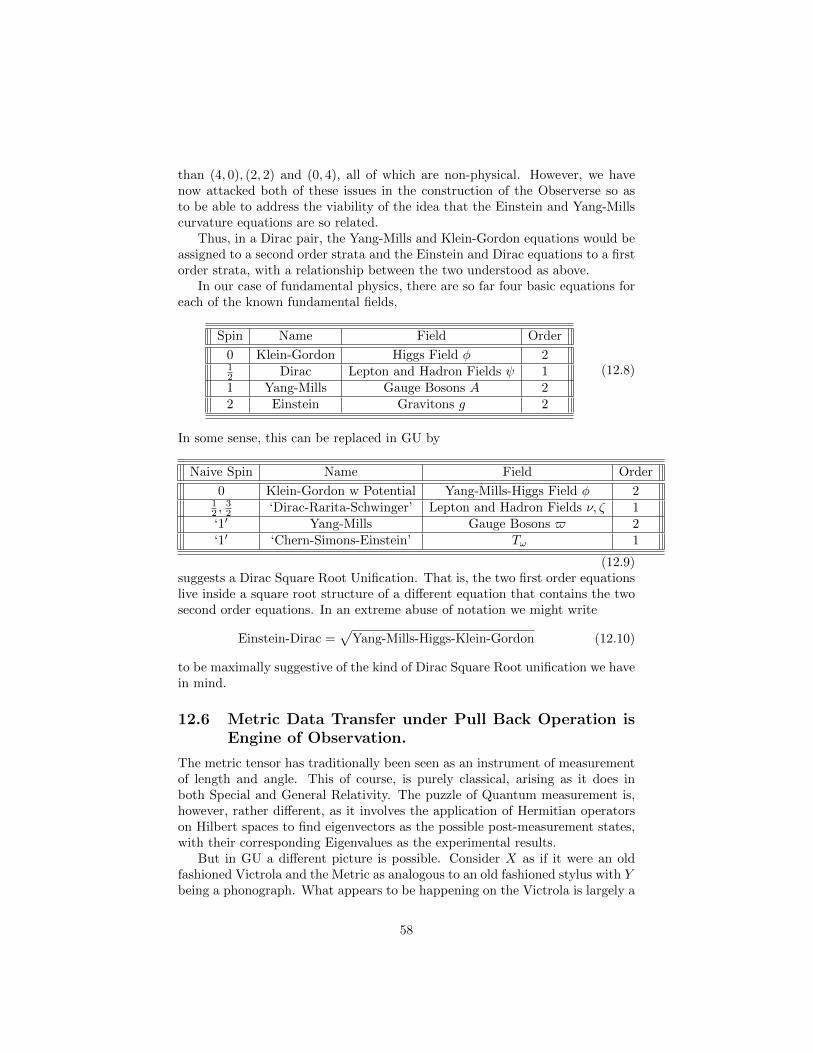
than (4, 0), (2, 2) and (0, 4), all of which are non-physical. However, we havenow attacked both of these issues in the construction of the Observerse so asto be able to address the viability of the idea that the Einstein and Yang-Millscurvature equations are so related.

Thus, in a Dirac pair, the Yang-Mills and Klein-Gordon equations would beassigned to a second order strata and the Einstein and Dirac equations to a firstorder strata, with a relationship between the two understood as above.

In our case of fundamental physics, there are so far four basic equations foreach of the known fundamental fields,

Spin Name Field Order

0 Klein-Gordon Higgs Field φ 212 Dirac Lepton and Hadron Fields ψ 11 Yang-Mills Gauge Bosons A 22 Einstein Gravitons g 2

(12.8)

In some sense, this can be replaced in GU by

Naive Spin Name Field Order

0 Klein-Gordon w Potential Yang-Mills-Higgs Field φ 212 ,

32 ‘Dirac-Rarita-Schwinger’ Lepton and Hadron Fields ν, ζ 1

‘1′ Yang-Mills Gauge Bosons $ 2‘1′ ‘Chern-Simons-Einstein’ Tω 1

(12.9)suggests a Dirac Square Root Unification. That is, the two first order equationslive inside a square root structure of a different equation that contains the twosecond order equations. In an extreme abuse of notation we might write

Einstein-Dirac =√

Yang-Mills-Higgs-Klein-Gordon (12.10)

to be maximally suggestive of the kind of Dirac Square Root unification we havein mind.

12.6 Metric Data Transfer under Pull Back Operation isEngine of Observation.

The metric tensor has traditionally been seen as an instrument of measurementof length and angle. This of course, is purely classical, arising as it does inboth Special and General Relativity. The puzzle of Quantum measurement is,however, rather different, as it involves the application of Hermitian operatorson Hilbert spaces to find eigenvectors as the possible post-measurement states,with their corresponding Eigenvalues as the experimental results.

But in GU a different picture is possible. Consider X as if it were an oldfashioned Victrola and the Metric as analogous to an old fashioned stylus with Ybeing a phonograph. What appears to be happening on the Victrola is largely a

58

Figure 6: Observation and The Observerse.

function of where the stylus alights on the phonograph. From the point of viewof the listener, each track or location on the phonograph is a different world,while from the perspective of the record manufacturer the album is a singleunified release. In this way, the world of states of Y is merely being sampledand displayed as if it were the only thing happening on X.

12.7 Spinors are Taken Chimeric and Topological to AllowPre-metric Considerations.

It has been very difficult to get upstream from Einstein’s concept of space-timefor a variety of reasons. In particular, the dependence of Fermions on the choiceof a metric in fact appears to doom us to beginning with the assumption of ametric if we wish to consider leptonic or hadronic matter. Yet this dependencemust be partially broken if we are to harmonize metric-generated gravity fromwithin metric-dependent Quantum Field Theory.

Many years ago, Nigel Hitchin demonstrated that, while the elliptic index ofa Dirac operator in Euclidean signature was an invariant by the Atiyah-Singerindex theorem, the dimension of the Kernel and Co-Kernel could jump undermetric variation. Since that time Jean-Pierre Bourguignon and others haveexpended a great deal of work tracking Spinors under continuous variation ofthe metric.

Given the odd way in which Spinors appear to be both intrinsically topo-logical (e.g. the topological A-genus) but confoundingly tied to the metric, wehave sought to search for the natural space over which the topological nature ofspinors is most clearly manifest. In essence, this has lead us to attempt to ab-sorb the metric structure into a new base space made of pure measuring devicesbut constructed from the purely topological representation of GL(r + s,R) on

the homogeneous spaces GL(r + s,R)/Spin(r, s)

59

12.8 Affine Space Emphasis Should Shift to A from MinkowskiSpace.

There appear to be many difficulties when attempting to do Quantum FieldTheory in curved space. Thus there has always been a question in the au-thor’s mind as to whether the emphasis on affine Minkowski space M1,3 is alinearized crutch to make the theorist’s model building easier, or whether thereis something actually fundamental about affine space analysis.

In some sense, GU attempts to split the difference here. We find the emphasison Minkowski space misplaced, but not the focus on affine theory, as no matterhow curved Space-time may be, there is always an affine space that is naturaland available with a powerful dictionary of analogies to relate it to ordinary andsuper-symmetric Quantum Field Theory:

Special Relativity/QFT to GU Relativity, QFT GU Analog

Affine Space M1,3 AModel Space R1,3 N = Ω1(ad)

Core Symmetries Spin(1, 3) H = Γ∞(PH ×Ad H)Inhomogeneous Poincare Group G

Extension = Spin(1, 3) nR1,3 = HnNFermionic Extension Space-Time SUSY (ν, ζ) ∈ Ω0(/S)⊕ Ω1(/S)

(12.11)This also makes more sense from the so-called super-symmetric perspective. If,historically, supercharges are to be thought of as square roots of translations,then in the context of a ‘superspace’ built not on M1,3 but on A, superchargeswould have an honest affine space to act and translate where they would ap-pear as square roots of operators or gauge potentials. This would also allow aframework where Supersymmetry12 could be formally active without the intro-duction of artificial superpartners which have been remarkable in their failureto materialize at expected energies. In this framework, the supercharges mayalready be here in the form of the ν and ζ fields as this would not be space-timesupersymmetry.

12.9 Chirality Is Merely Effective and Results From De-coupling a Fundamentally Non-Chiral Theory

Consider a stylized system of equations for a world Y with metric g, havingscalar curvature R(y), and endowed with a non-chiral Dirac operator operatingon full Dirac Spinors,(−Λ(y) /∂A/∂A −Λ(y)

)(ψL(y)ψR(y)

)= 0 R(y)

(1 00 1

)= 4

(Λ(y) 0

0 Λ(y)

)(12.12)

12The author finds supersymmetry unnecessarily confusing as an as-if symmetry and isuncomfortable saying much more about it.

60

which are nonetheless decomposed into chiral Weyl component-spinors. Solvingboth of these equations together yields a system of coupled equations:

/∂AψL(y) =R(y)

4ψR(y) (12.13)

/∂AψR(y) =R(y)

4ψL(y) (12.14)

leading to a stylized massive Dirac Equation with mass m = R(y)4 for any fixed

background metric for which the scalar curvature R(y) is approximately con-stant in a region under study.

However, in any region where the scalar curvature was zero or sufficientlyclose to zero,

R(y) ≈ 0 (12.15)

the differential equations would decouple as they are only linked by the scalarcurvature term of order zero.

/∂AψL(x) ≈ 0 (12.16)

/∂AψR(y) ≈ 0 (12.17)

This however, is not the end of the story when the tangent bundle has furtherstructure. In the neighborhood of an embedding such as we have in:

ג : X1,3 −→ Y 7,7 (12.18)

we haveTY)∗ג 7,7) = TX1,3 ⊕N6,4

ג (12.19)

from our previous discussion.However at the level of the chiral Weyl halves of the total Dirac Spinor we

have two decompositions:

S64/)∗גL (TY )) =

Luminous Light Standard Model Family Matter︷ ︸︸ ︷(/S

2L(TX)⊗ /S

16L (Nג))⊕ (/S

2R(TX)⊗ /S

16R (Nג))

S64/)∗גR (TY )) = (/S

2L(TX)⊗ /S

16R (Nג))⊕ (/S

2R(TX)⊗ /S

16L (Nג))︸ ︷︷ ︸

Dark Decoupled Looking Glass Matter

(12.20)

requiring a different view of chirality as both Left and Right handed spinorsemerge from the branching rules of both Weyl halves confusing the picture.Left handed spinors on Y do not remain exclusively Left handed on X.

It may be asked what the relevance of the above stylized toy example is tothe model under discussion. Quite simply, for every field on Y in the Observerse,there is both a naive spin and a true spin. The naive spin of a differential formvalued in another bundle is taken to be the spin of the form field if the tensored

61

bundle were taken formally to be purely auxiliary. Thus, for example, an ad-valued one form would carry naive spin 1 whether or not the ad bundle wasderived from the structure bundle of the base space on which it lives.

Thus, for example, our bundle Ω1(Y, ad) of ad-valued 1-forms has naive spinone, but this disguises the fact that it also contains an invariant subspace thatderives from Λ1 ⊗ Λ1 ⊂ Λ1 ⊗ Λ∗. This space of naive spin 1 would appear tobe truly spinless from the point of view of Y . Thus, in some sense, the fieldplaying the role of the fundamental mass for the generalized Dirac equations isactually part of the gauge potential. This sets up a three way linkage:

Cosmological ‘Constant’ Λ↔ Spinless Gauge Field↔ Fermion Mass (12.21)

and it is in such ways that GU seeks to attack non-anthropic fine tuning prob-lems by having the same fields do multiple service.

In essence here, a fundamentally non-chiral world of Dirac Spinors in thissimplified example would appear chiral in regions of low scalar gravity. Frombeings made of such chiral matter, they would naturally view the universe asbeing mildly chiral much the way each of the two hands in Escher’s drawing isseparately approximately symmetric about its middle digit. But raised high, thesymmetry breaks down as digits two and four are only approximately symmetricin most people, and one and five are undeniably different. Yet it is not onlythe two middle fingers which are beautiful and symmetric about themselves,because the proper symmetry is left pinky to right pinky, left thumb to rightthumb etc. and not left pinky to left thumb, right pinky to right thumb whichis not broken as a symmetry, but simply accidental as well as being false.

12.10 Three Generations Should be Replaced by 2+1 modelof two True Generations and one Effective ImposterGeneration

At the time of this writing, the author is not convinced that we have three truegenerations of matter which differ only by mass. We instead posited here thatthe so-called third generation of matter is instead part of pure Rarita-SchwingerSpin− 3

2 matter on Y and its Spin− 12 appearance on X is the result of branching

rules under pull back from Y where it is native:

R(TY/)∗ג )) = /R(ג∗(TY )) = /R(TX ⊕Nג) =

/R(TX)⊗ /S(Nג)⊕

/S(TX)⊗ /R(Nג)⊕

/S(TX)⊗ /S(Nג)︸ ︷︷ ︸Imposter Third Generation

(12.22)

Thus, part of the field ζ ∈ Ω1(Y, /SR) is an ordinary second generation spinorin Ω0(Y, /SL) via the Dirac gamma matrix contraction while the complement/RR(TY ) corresponding to the sum of the highest weights contains the imposter

62

third generation which is only revealed under decomposition as in the above.Thus, it is not a true generation as it has a different representation structurethan the other two beyond its obvious mass difference.13

12.11 Final Thoughts

To sum up, let us revisit the Witten synopsis to see what GU has to say aboutit:

Figure 7: Edward Witten Synopsis.

As we have seen, Geometric Unity may be considered an alternative narra-tive that tweaks familiar concepts in various ways. As the author sees it, it isreally a collection of interconnected ideas about shifting our various perspec-tives. Given the apparent stagnation in the major programs, GU has soughtan alternate interpretation of either or both of the two incompatible modelsfor fundamental physics of the Standard Model or General Relativity. In ouropinion this represents a rather general perspective on the likely reasons forthe impasse in fundamental physics encountered over the five decades since theearly 1970s. At almost every level, it appears to us as if the instantiations of themost important general ideas and insights hardened prematurely into assump-tions that now block progress. In most cases, our shift in perspective is usuallynot a rejection of the current models at the level of ideas so much as a rejec-tion of the pressure to communicate ideas concretely through instantiations. Inessence, we see an intellectual disagreement between the tiny group of physi-cists who have sought to discover physical law and the vast majority of theoristswho attempted to work out its consequences. What good is a beauty principlethat works only in the hands of Einstein, Dirac, Yang, and a handful of others,while leading to failure and madness for others? Yet, in these matters, we havecome to side with Dirac’s widely misunderstood perspective on the relationshipbetween, instantiation, beauty, theory and experiment. In essence, a beautiful

13Note: we are speaking loosely here as if mass eigenstates and flavor eigenstates were oneand the same.

63

theory is not its instantiation, but those who do not seek physical law cannotbe forced to accept this critical issue.

To rephrase Witten’s paragraph then in light of Geometric Unity, it mightbe rewritten as follows:

“To Summarize the strongest claims of the strongest form of Ge-ometric Unity, the basic assertions would be: i) Space-time X1,3

arises as a pseudo-Riemannian manifold from maps ג between two

spaces Xn and Yn2+3n

2 (X) = Met(X) where Y is constructed fromX at a topological level. ii) Over Y is a bundle C with a naturalmetric which is (semi-canonically) isomorphic to TY , and one whosestructure bundle carries a complex representation

Spin(n2 + 3n

2,C) −→ U(2

n2+3n4 ,C) (12.23)

on Dirac spinors with structure bundle PH for H a real form ofU , with no internal symmetry groups. There is an inhomogeneousextension G of the gauge group H of PH acting on the space of con-nections A(PH) where the stabilizer of any point A0 ∈ A gives riseto a non-trivial endomorphism τA0 : H −→ G. iii) Fermions on X4

are pullbacks (ν)∗ג and (ζ)∗ג of unadorned non-chiral Dirac spinorsν ∈ Ω0(Y, /S) and 1-form valued spinors, ζ ∈ Ω1(Y, /S) on Y . In lowgravitational regimes, the equations governing the fractional spinfields decouple leading to emergent effective chirality that disguisesthe non-chiral fundamental theory, and leading to Witten’s repre-sentations R and R which are not isomorphic exactly as accordingto the branching rules for Spinors. The cosmological constant is ac-tually the Vacuum Expectation Value (VEV) of a Field which playsthe role of a fundamental mass, leading to the light Fermions beinglight in low gravity regimes. iv) If Super-symmetry is considered,it lives on the inhomogeneous gauge group and not the inhomoge-neous Lorentz or Poincare group where gauge potentials take overfrom Galilean transformations and the affine space A plays the roleof the Minkowski space M1,3. The lack of internal symmetries in-dicates why naive super-partners have not been seen as space-timeSUSY may be implementing over the wrong group. v) Gravity גlives on X while the fields of the standard model are native to Yleading to a reason for General Relativity to appear classical on Xin contrast to the Quantum nature of the SM fields ω tied to Y . vi)Gravity is the engine of observation, so that where gravity is local-ized in different sections ,aג ,bג it pulls back different content whilevii) Gravity on Y is replaced by a cohomological theory involving anobstruction δ2

ω = Υ combining elements of Einstein-Grossman, Diracand Chern-Simons theories, while there is a new 2nd order theoryreplacing Yang-Mills, Higgs and Klein-Gordon theories so that thecohomological theory δ2

ω = Υ = 0 is a ‘Dirac square root’ of the

64

second order theory. viii) The branching rules of ν leads to the ap-pearance of one family of Fermions. ix) ζ branches as a second familydue to gamma matrix multiplication on Y as TY ⊗ /SY = /SY ⊕ /RYwith a Rarita-Schwinger remainder. The Spin 3

2 portion of ζ breaksdown under pull back to reveal a third ‘imposter generation’ thatis merely effective, as it has different representation behavior in thefull theory. x) The first order theory has a rich moduli of classicalsolutions and Υ = 0 carries an elliptic deformation complex in Eu-clidean signature once the redundant Euler-Lagrange equations arediscarded.14”

We would like to end this speculative foray with a quote from the man whosequestion provided the impetus for this excursion.

“The relativity principle in connection with the basic Maxwellianequations demands that the mass should be a direct measure of theenergy contained in a body; light transfers mass. With radium thereshould be a noticeable diminution of mass.The idea is amusing andenticing; but whether the almighty is laughing at it and is leadingme up the garden path — that i cannot know.” -Albert Einstein

While we believe in the story of Geometric Unity, we find the above, now asthen, to be sage words in all such endeavors.

Appendix: Other Elements of Shiab Construc-tions

Continuing on from our earlier discussion of Shiab operator construction, theauthor simply wanted to note some of the gadgetry that has come up in theconstruction of these operators in past years. Most of this is obvious, but thefact that there are two products on the Unitary group Lie algebras given bymatrix commutators, and anti-commutators multiplied by i, is an example ofsomething that can be easily forgotten. The author may have forgotten othertools in the Shiab workshop over the years as well.

Wedge

The wedge product passes to bundle valued forms from the usual DeRhamcomplex.

Hodge Star

As we have assumed our manifold to be oriented from the beginning, everytime a metric g on Y is chosen it induces a non-vanishing volume form dvol

14The so-called Seiberg-Witten equations were first found this way around 1987 as thesimplest toy model to proxy this moduli problem.

65

compatible with the metric and orientation. This in turn induces a Hodge Staroperator

∗ : Ωi(B) −→ Ωd−i(B) (12.24)

which passes to forms valued in arbitrary bundles B over Y .

Contraction

Various forms of contraction can be defined either with co-variant against con-travariant tensors in the obvious way or via the wedge and star operationsbetween forms as in:

φ ∨ µ = ∗(φ ∧ ∗µ) (12.25)

Adjoint Bundle

Bracket

As with any Lie Group, U(64, 64) carries a Lie Bracket structure. Given thatit lives embedded within the Clifford Algebra ClC(7, 7) = C(128), it can beconstructed from the matrix algebra product in the usual fashion:

[a, b] = a · b− b · a (12.26)

Symmetric Product

Unlike most Lie Algebras, there is a second symmetric product on u(n) gottenfrom taking:

a, b = i(a · b+ b · a) (12.27)

Volume Form

The analog of the Hodge Star operator is multiplication with the Clifford Volumeform λ.

Appendix: Thoughts on Method

A few words are in order about what the author sees as unbridgeable differenceswith the mainstream of the community of professional physicists.

Experiment and The Scientific Method

The author understands the scientific method differently from many others andparticularly from many within the world of String Theory. In essence there aregeneral ideas and multiple instantiations of those ideas. The author believesthat many who put their faith in the scientific method do not understand thedanger of being pressured to discard ideas because one of their instantiationswas invalidated by experiment. This is, in essence, the very point Dirac raised

66

in his 1963 Scientific American Article where he warned that beauty rather thanthe scientific method should be used as a guide to progress:

“It seems that if one is working from the point of view of gettingbeauty in one’s equations, and if one has really a sound insight, oneis on a sure line of progress. If there is not complete agreement be-tween the results of one’s work and experiment, one should not allowoneself to be too discouraged, because the discrepancy may well bedue to minor features that are not properly taken into account andthat will get cleared up with further developments of the theory.”

It is the misinterpretation of this very clear point that the author findschilling. Dirac was clearly not saying that if a theory is beautiful, it need notagree with experiment, and yet he is frequently lampooned as such. Why isthis?

The author believes there is a principle, by which the scientific communitiespush most members for hyper explicit claims so as to learn the general ideaand to wed the author to a prediction that can be easily falsified. Should theauthor succumb to associating her or his more general idea with a particularinstantiation that fails to be confirmed, that idea is now ‘up for grabs’. Fur-ther, established players can speak more generally allowing different membersdifferent privileges.

The author is proud to be able to offer algebraic predictions as to the ‘internalquantum numbers’ of new particles but would need the help of Quantum FieldTheorists to see whether these can be sharpened further to include energy scales.The author is not equipped to undertake that effort alone but considers thepredictions already offered to be considerably more explicit than many of thecurrent contenders for a theory of everything on a relative basis. The author’sexperience is that in calling such quantum numbers ‘predictions’ is that thosefarthest away from making such predictions are paradoxically the most likelyto complain viciously about the lack of an energy threshold so as to deflectcriticism from their own theory’s failure to be able to make such claims.

Isolation

It is the experience of this author that almost no professional mathematiciansand physicists have any concept what it is like to be isolated from the communityfor 20 years or more at a time. Geometry and field theory are languages that inthis author’s experience, decay exceedingly rapidly when there is no one withwhich to speak them, and it is nearly impossible to find it actively maintainedanywhere outside of the profession.

It has been over 25 years since the current author was in a professionalenvironment where anyone else was conversant in the topics discussed here. Myapologies are offered for any inconvenience caused, but the author’s ability toconverse with the professional community, but, in full candor, the ability tocommunicate was likely to get even further degraded via additional years ofisolation.

67

Appendix: Locations Within GU

We collect here for convenience the usual ingredients that constitute fundamen-tal physics and give their intended address within the framework of GeometricUnity.

Usual Name GU Location

Higgs Field ($)∗גSM 1st Generation Fermions (νL)∗ג

SM 2nd Generation Fermions ζ)∗ג /SR)

SM 3rd Generation Fermions ζ)∗ג /RR )Gluons ((גN)Spin(6)$)∗ג

Weak Isospin ((גN)Spin(4)$)∗גWeak Hypercharge ((גN)Spin(6)×Spin(4)$)∗גSpace-time Metric ג

Higgs Potential < Υω,Υω >CKM Matrix ($)∗ג

Einstein Field Equations Υω = 0Dirac Equations Υω = 0

Yang-Mills-Maxwell Equations D∗ωΥω = 0Higgs Klein-Gordon D∗ωΥω = 0

Cosmological Constant ($)∗ג as a VEVYukawa Couplings χ)∗ג /Dωχ) as a VEV

(12.28)

68

References

[1] D. Bar-Natan and E. Witten, “Perturbative expansion of Chern-Simonstheory with noncompact gauge group,” Commun. Math. Phys. 141, 423(1991).

[2] A. L. Besse, Einstein manifolds, Ergebnisse der Mathematik und ihrerGrenzgebiete, Band 10, Springer-Verlag, Berlin, Heidelberg, New York,London, Paris, Tokyo, 1987, xii + 510 pp.,ISBN 3-540- 15279-2

[3] P. Dirac, “The Evolution of the Physicist’s Picture of Nature,” ScientificAmerican, May 1963, Vol. 208, Number 5, pg. 45-53.

[4] M. Gell-Mann, “From renormalizability to calculability?,” in Shelter IslandII, 1983, Proceedings, Quantum Field Theory and The Fundamental Prob-lems Of Physics, 3-23, R. Jackiw, N. N. Khuri, S. Weinberg, and E. Witten,eds. Dover Publications, 1986.

[5] R. Harvey, Spinors and Calibrations. Perspectives in Mathematics, 9. Aca-demic Press, New York, 1990.

[6] H. B. Lawson and M.-L. Michelson, “Spin Geometry,” Princeton UniversityPress, Princeton, 1989.

[7] C. W. Misner, K. S. Thorne and J. A. Wheeler, “Gravitation,”,isbn 978-0-7167-0344-0, 978-0-691-17779-3, ”W. H. Freeman”, ”San Francisco”,”1973”

[8] E. Weinstein, Extension of self-dual Yang-Mills equations across the 8th di-mension, Ph.D. dissertation, Harvard University Mathematics Department,1992

[9] E. Weinstein, Geometric Unity, In Preparation.

[10] E. Weinstein, A Portal Special Presentation- Geometric Unity: A FirstLook, April 1, 2020, YouTube.

[11] E. Witten, ‘Physics and Geometry’, Proc. Intern. Congr. Math. 1986(Berkeley) (Amer. Math. Soc., Providence, 1987).

[12] P. Woit, 2006, Not Even Wrong: the failure of string theory and the searchfor unity in physical law. Basic Books, New York, 2006.

69