Geometric Structures in Dimension two
174
Geometric Structures in Dimension two Bjørn Jahren August 11, 2015
Transcript of Geometric Structures in Dimension two

Geometric Structures in Dimension two
Bjørn Jahren
August 11, 2015

2

Contents
1 Hilbert’s axiom system 1
2 Hyperbolic geometry 112.1 Stereographic projection. . . . . . . . . . . . . . . . . . . . . 132.2 Congruence in H; Mobius transformations . . . . . . . . . . . 192.3 Classification of real Mobius transformations . . . . . . . . . 292.4 Hilbert’s axioms and congruence in H . . . . . . . . . . . . . 392.5 Distance in H . . . . . . . . . . . . . . . . . . . . . . . . . . . 432.6 Angle measure. H as a conformal model . . . . . . . . . . . . 472.7 Poincare’s disk model D . . . . . . . . . . . . . . . . . . . . . 492.8 Arc–length and area in the hyperbolic plane . . . . . . . . . . 562.9 Trigonometry in the hyperbolic plane . . . . . . . . . . . . . . 65Appendix. Remarks on the Beltrami–Klein model . . . . . . . . . 73
3 Classification of surfaces 81
4 Geometry on surfaces 934.1 Introduction, local structure . . . . . . . . . . . . . . . . . . . 934.2 Geometric structure on surfaces . . . . . . . . . . . . . . . . . 95
5 Differential geometry 1035.1 Tangent planes and derivatives of maps . . . . . . . . . . . . 1055.2 Orientation . . . . . . . . . . . . . . . . . . . . . . . . . . . . 1125.3 Riemannian surfaces . . . . . . . . . . . . . . . . . . . . . . . 1165.4 Isometries . . . . . . . . . . . . . . . . . . . . . . . . . . . . . 1215.5 Curvature . . . . . . . . . . . . . . . . . . . . . . . . . . . . . 1255.6 Geodesics . . . . . . . . . . . . . . . . . . . . . . . . . . . . . 1375.7 Geodesic polar coordinates . . . . . . . . . . . . . . . . . . . 1485.8 Riemannian surfaces of constant curvature . . . . . . . . . . . 1545.9 The Gauss–Bonnet theorem . . . . . . . . . . . . . . . . . . . 156
i

ii CONTENTS
Index 169
Chapter 1
Hilbert’s axiom system forplane geometry;A short introduction
Euclid’s “Elements” introduced the axiomatic method to geometry, and formore than 2000 years this was the main textbook for students of geometry.But the 19th century brought about a revolution both in the understandingof geometry and of logic and axiomatic method, and it became more andmore clear that Euclid’s system was incomplete and could not stand up tothe modern standards of rigor. The most famous attempt to rectify this wasmade by the great German mathematician David Hilbert, who published anew system of axioms in his book “Grundlagen der Geometrie” in 1898. Herewe will give a short presentation of Hilbert’s axioms with some examplesand comments, but with no proofs. For more details, we refer to the richliterature in this field — e. g. the books ”Euclidean and non-Euclideangeometries” by M. J. Greenberg and ”Geometry: Euclid and beyond” by R.Hartshorne.
Hilbert also treats geometry in 3-space, but we will only consider the2-dimensional case. The basic objects of our study are then points andlines in a plane. At the outset the plane is just a set S where the elementsP are called points. The lines are, or can at least be naturally identifiedwith certain subsets l of S, and the fundamental relation is the incidencerelation P ∈ l, which may or may not be satisfied by a point P and a linel. But we also introduce two additional relations: betweenness, enabling usto talk about points lying between two given points, and congruence, whichis needed when we want to compare configurations in different parts of the
1

2 CHAPTER 1. HILBERT’S AXIOM SYSTEM
plane. Hilbert formulated three sets of axioms for these relations: incidenceaxioms, betweenness axioms and congruence axioms. In addition to thesewe also need an axiom of continuity to make sure that lines and circles have“enough” points to intersect as they should, and of course the axiom ofparallels. As we introduce Hilbert’s axioms, we will gradually put more andmore restrictions on these ingredients, and in the end they will essentiallydetermine the geometry of the Euclidean plane uniquely.
Note that although circles also are important objects of study in classicalplane geometry, we do not have to postulate them, since, as we shall see,they can be defined in terms of the other notions.
Before we start, maybe a short remark about language is in order: Anaxiom system is a formal matter, but the following discussion will not bevery formalistic. After all, the goal is to give a firm foundation for mattersthat we all have a clear picture of in our minds, and as soon as we haveintroduced the various formal notions, we will feel free to discuss them inmore common language. For example, although the relation P ∈ l should,strictly speaking, be read: “P and l are incident”, we shall use “l containsP”, “P lies on l” or any obviously equivalent such expression.
We are now ready for the first group of axioms, the incidence axioms:
I1: For every pair of distinct points A and B there is a unique line lcontaining A and B.
I2: Every line contains at least two points.
I3: There are at least three points that do not lie on the same line.
We let AB denote the unique line containing A and B.
These three axioms already give rise to much interesting geometry, so-called “incidence geometry”. Given three points A, B, C, for example,any two of them span a unique line, and it makes sense to talk about thetriangle ABC. Similarly we can study more complicated configurations.The Cartesian model R2 of the Euclidean plane, where the lines are the setsof solutions of nontrivial linear equations ax+by = c, is an obvious example,as are the subsets obtained if we restrict a, b, c, x, y to be rational numbers(Q2), the integers (Z2), or in fact any fixed subring of R (requiring now alsothat lines are nonempty). However, spherical geometry, where S is a sphereand the lines are great circles, is not an example, since any pair of antipodalpoints lies on infinitely many great circles — hence the uniqueness in I1

3
does not hold. This can be corrected by identifying every pair of antipodalpoints on the sphere. Then we obtain an incidence geometry called the (real)projective plane P2. One way to think about the points of P2 is as linesthrough the origin in R3. If the sphere has center at the origin, such a linedetermines and is determined by the antipodal pair of points of intersectionbetween the line and the sphere. A “line” in P2 can then be thought of asa plane through the origin in R3, since such a plane intersects the sphereprecisely in a great circle. Notice that in this interpretation the incidencerelation P ∈ l corresponds to the relation “the line l is contained in theplane P”.
There are also finite incidence geometries — the smallest has exactlythree points where the lines are the three subsets of two elements.
The next group of axioms deals with the relation “B lies between A andC”. In Euclidean geometry this is meaningful for three points A, B and Clying on the same straight line. The finite geometries show that it is notpossible to make sense of such a relation on every incidence geometry, sothis is a new piece of structure, and we have to declare the properties weneed. We will use the notation A ∗B ∗ C for “B lies between A and C”.
Hilbert’s axioms of betweenness are then:
B1: If A∗B∗C, then A, B and C are distinct points on a line, and C∗B∗Aalso holds.
B2: Given two distinct points A and B, there exists a point C such thatA ∗B ∗ C.
B3: If A, B and C are distinct points on a line, then one and only one ofthe relations A ∗B ∗ C, B ∗ C ∗A and C ∗A ∗B is satisfied.
B4: Let A, B and C be points not on the same line and let l be a line whichcontains none of them. If D ∈ l and A ∗D ∗ B, there exists an E onl such that B ∗E ∗C, or an F on l such that A ∗ F ∗C, but not both.
If we think of A, B and C as the vertices of a triangle, another formula-tion of B4 is this: If a line l goes through a side of a triangle but none of itsvertices, then it also goes through exactly one of the other sides. This for-mulation is also called Pasch’s axiom. The uniqueness (the word ”exactly”)is actually not necessary here, as it can be shown to be a consequence of theother axioms. Note that B4 does not hold in Rn for n ≥ 3. Hence I3 andB4 together define the geometry as ’2–dimensional’.

4 CHAPTER 1. HILBERT’S AXIOM SYSTEM
In the standard Euclidean plane (and in other examples we shall studylater) we can use the concept of distance to define betweenness. Namely,we can then define A ∗ B ∗ C to mean that A, B are C are distinct andd(A,C) = d(A,B) + d(B,C), where d(X,Y ) is the distance between X andY . (Check that B1-4 then hold!) This way Q2 also becomes an example,but not Z2, since B4 is not satisfied. (Exercise 3.)
Observe also that every open, convex subset K of R2 (e. g. the interiorof a circular disk) satisfies all the axioms so far, if we let the “lines” bethe nonempty intersections between lines in R2 and K, and betweenness isdefined as in R2. (This example will be important later.) The projectiveplane, however, can not be given such a relation. The reason is that in thespherical model for P2, the “lines” are great circles where antipodal pointshave been identified, and these identification spaces can again naturally beidentified with circles. But if we have three distinct points on a circle, eachof them can equally well be said to lie “between” the others. Therefore B3can not be satisfied.
The betweenness relation can be used to define the segment AB as thepoint set consisting of A, B and all the points between A and B:
AB = A,B ∪ C|A ∗ C ∗B.
Similarly we can define the ray−−→AB as the set
−−→AB = AB ∪ C|A ∗B ∗ C.
If A, B and C are three point not on a line, we can then define the angle
∠BAC as the pair consisting of the two rays−−→AB and
−→AC.
∠BAC = −−→AB,
−→AC.
Note also that AB =−−→AB ∪
−−→BA.
Betweenness also provides us with a way to distinguish between the twosides of a line l. We say that two points A and B are on the same side of lif AB ∩ l = ∅. It is not difficult to show, using the axioms, that this is anequivalence relation on the complement of l, and that there are exactly twoequivalence classes: the two sides of l. (Exercise 4.) Similarly we say thata point D is inside the angle ∠BAC if B and D are on the same side ofAC, and C and D are on the same side of AB. This way we can distinguishbetween points inside and outside a triangle. We also say that the angles
∠BAC and ∠BAD are on the same (resp. opposite) side of the ray−−→AB if
C and D are on the same (resp. opposite) side of the line AB.

5
The same idea can also be applied to distinguish between the points ona line on either side of a given point. Using this, one can define a linearordering of all the points on a line. Therefore the axioms of betweenness aresometimes called “axioms of order”.
We have now introduced some of the basic concepts of geometry, but weare missing an important ingredient: we cannot yet compare two differentconfigurations of points and lines. To achieve this, we need the fundamentalnotion of congruence. Intuitively, we may think of two configurations ascongruent if there is some kind of “rigid motion” which moves one ontothe other. In the Euclidean plane R2 this can be defined in terms of anglemeasures and distances, such that two configurations are congruent if alltheir ingredients are “of the same size”. However, this has no meaning onthe basis of just the incidence- and betweenness axioms. Hence congruencehas to be introduced as yet another piece of structure — a relation whoseproperties then must must be defined by additional axioms.
There are two basic notions of congruence — congruence of segmentsand congruence of angles. Congruence of more general configurations canthen be defined as a one-one correspondence between the point sets involvedsuch that all corresponding segments and angles are congruent. We use thenotation AB ∼= CD for “the segment AB is congruent to the segment CD”,and similarly for angles or more general configurations. Hilbert’s axioms forcongruence of segments are:
C1: Given a segment AB and a ray r from C, there is a uniquely deter-mined point D on r such that CD ∼= AB.
C2: ∼= is an equivalence relation on the set of segments.
C3: If A ∗ B ∗ C and A′ ∗ B′ ∗ C ′ and both AB ∼= A′B′ and BC ∼= B′C ′,then also AC ∼= A′C ′.
If betweenness is defined using a distance function (as in the Euclideanplane) we can define AB ∼= CD as d(A,B) = d(C,D). C2 and C3 are thenautomatically satisfied, and C1 becomes a stronger version of B2.
Even without a notion of distance we can use congruence to compare“sizes” of two segments: we say that AB is shorter than CD (AB < CD) ifthere exists a point E such that C ∗ E ∗D and AB ∼= CE.
We can now also define what we mean by a circle: Given a point O anda segment AB, we define the circle with center O and radius (congruent to)

6 CHAPTER 1. HILBERT’S AXIOM SYSTEM
AB as the point set C ∈ S |OC ∼= AB. Note that this set is nonempty:C1 implies that any line through O intersects the circle in two points.
The axioms for congruence of angles are:
C4: Given a ray−−→AB and an angle ∠B′A′C ′, there are angles ∠BAE and
∠BAF on opposite sides of AB such that ∠BAE ∼= ∠BAF ∼= ∠B′A′C ′.
C5: ∼= is an equivalence relation on the set of angles.
C6: Given triangles ABC and A′B′C ′. If AB ∼= A′B′, AC ∼= A′C ′ and∠BAC ∼= ∠B′A′C ′, then the two triangles are congruent — i. e. BC ∼=B′C ′, ∠ABC ∼= ∠A′B′C ′ and ∠BCA ∼= ∠B′C ′A′.
C4 and C5 are the obvious analogues of C1 and C2, but note that C4says that we can construct an arbitrary angle on both sides of a given ray.C6 says that a triangle is determined up to congruence by any angle andits adjacent sides. This statement is often referred to as the “SAS” (side–angle–side) congruence criterion.
In the Euclidean plane R2 we define congruence as equivalence underactions of the Euclidean group of transformations of R2. This is generatedby rotations and translations, and can also be characterized as the set oftransformation of R2 which preserve all distances. It is quite instructive toprove that the congruence axioms hold with this definition.
These three groups contain the most basic axioms, and they are sufficientto prove a large number of propositions in book I of “Elements”. However,when we begin to study circles and “constructions with ruler and compass”,we need criteria saying that circles intersect (have common points) withother circles or lines when our intuition tells us that they should. The nextaxiom provides such a criterion.
First a couple of definitions:
Definition: Let Γ be a circle with center O and radius OA. We say thata point B is inside Γ if OB < OA and outside if OA < OB.
We say that a line or another circle is tangent to Γ if they have exactlyone point in common with Γ.
We can now formulate Hilbert’s axiom E :
E: Given two circles Γ and ∆ such that ∆ contains points both inside andoutside Γ. Then Γ and ∆ have common points. (They “intersect”.)

7
(It follows from the other axioms that they will then intersect in exactlytwo points.) This is an example of what we call a continuity axiom. Thefollowing variation is actually a consequence of axiom E:
E’: If a line l contains points both inside and outside the circle Γ, then land Γ will intersect. (Again in exactly two points.)
Hilbert gives the Axiom of parallels the following formulation — oftencalled “Playfair’s axiom” (after John Playfair i 1795, although apparently itgoes back to Proclus in the fifth century):
P: (Playfair’s axiom) Given a line l and a point P not on the line. Thenthere is at most one line m through P which does not intersect l.
If the lines m and l do not intersect, we say that they are parallel, andwe write m ‖ l. The existence of a line m through P parallel to l can beshown to follow from the other axioms, so the real content of the axiom isthe uniqueness.
With these axioms we are able to prove all the results in Euclid’s “Ele-ments” I–IV, but they do not yet determine the Euclidean plane uniquely.The standard plane (R2 with the structure defined so far) is an example,and it is an instructive exercise to prove this in detail, but we obtain otherexamples by replacing the real numbers by another ordered field where ev-ery element has a square root! For uniqueness we need a stronger continuityaxiom, as for instance Dedekind’s axiom:
D: If a line l is a disjoint union of two subset T1 and T2 such that all thepoints of T1 are on the same side of T2 and vice versa, then there isa unique point A ∈ l such that if B1 ∈ T1 and B2 ∈ T2, then eitherA = B1, A = B2 or B1 ∗A ∗B2.
This is a completeness axiom with roots in Dedekind’s definition of thereal numbers, and an important consequence is that the geometry on anyline can be identified with the geometry on R. One can show that it impliesaxiom E, and together with the groups of axioms I*, B*, C* and P it doesdetermine Euclidean geometry completely.
Finally we mention that axiom D also implies another famous continuityaxiom, the Axiom of Archimedes:

8 CHAPTER 1. HILBERT’S AXIOM SYSTEM
A: Given two segments AB and CD, we can find points C = C0, . . . , Cnon−−→CD, such that CiCi+1
∼= AB for every i < n and CD < CCn.
(“Given a segment AB, then every other segment can be covered by afinite number of congruent copies of AB”.)
Using this axiom we can introduce notions of distance and length suchthat AB has length one, say, and a geometry with the axioms I*, B*, C* P,E and A can be identified with a subset of the standard Euclidean plane.
Exercises.
1. Find all incidence geometries with four or five points.
2. Let V be a vector space of dimension at least 2 over a field F . Showthat V satisfies I1-3, if we define lines to be sets of the form A+tB|t ∈F, where A,B ∈ V , B 6= 0.
3. Show that Q2 satisfies axioms B1–4, but Z2 does not.
4. Prove that ’being on the same side of the line `’ is an equivalencerelation on the complement of `, with exactly two equivalence classes.
5. Let A and B be distinct points in a geometry satisfying axioms I1–3and B1–4. Show that we can find a point C such that A ∗ C ∗B.
6. Consider a triangle ABC and a line ` not containing any of the vertices.Show that ` cannot intersect all three sides AB, BC and AC.
Why does this prove uniqueness in Pasch’s axiom (B4)?
7. Assume A ∗B ∗C and B ∗C ∗D. Show that A ∗B ∗D and A ∗C ∗D.
8. Show that Q2 does not satisfy C1. Try to determine conditions on analgebraic extension F of Q such that F 2 will satisfy C1.
9. Show that the center of a circle is uniquely determined.
10. Discuss which axioms are needed in order to bisect a given segment.
11. Which axioms are satisfied by Q 2, where Q is the algebraic closure of
Q?

9
12. Show that the axiom of Archimedes can be used to define a lengthfunction on segments.
13. Suppose given a geometry with incidence, betweenness and congru-ence, and let r be a ray with vertex O. Let ` be the unique linecontaining r.
Show that we can give ` the structure of an ordered abelian group,with O as neutral element and such that P > O if and only if P ∈ r.
Show that two different rays give rise to isomorphic ordered groups.
14. Give the vector space R2 its standard inner product. Show that amap φ : R2 → R2 preserves distances if and only if it can be writtenφ(x) = Ax+ b, where A is an orthogonal 2×2 matrix and b is a vector.

10 CHAPTER 1. HILBERT’S AXIOM SYSTEM

Chapter 2
An introduction tohyperbolic geometry
Introduction.
Among Euclid’s axioms, the parallel axiom has always been the one causingthe most trouble. Already from the beginning it was recognized as lessobvious than the other axioms, and during more than two thousand yearsof fascinating mathematical history, geometers were trying to either prove itfrom the other axioms, or replace it by something more obvious but with thesame consequences. Today we know that the reason they did not succeed,is that there exist geometries where the axiom is not satisfied, but wherethe remaining axioms are still valid. One may wonder why this was notrealized earlier, but we must remember that geometry throughout all thistime was concerned with a description of the world “as it is”, and in the realworld a statement like the parallel axiom must either be true or not true.Euclid’s axioms do not define geometry; they describe more precisely whatkind of arguments we are allowed to use when proving new results aboutthe geometry of the world around us.
But in the 19th century the development of mathematics and mathemat-ical thinking finally brought freedom from this purely descriptive approachto geometry, allowing mathematicians like Lobachevski, Bolyai and Gaussto realize that one might construct perfectly valid geometries where all theother axioms of Euclid hold, but where the parallel axiom fails.
The first concrete such models were constructed by Beltrami in 1868, andmost of the models we shall present here are due to him, even if some of them
11

12 CHAPTER 2. HYPERBOLIC GEOMETRY
have names after other mathematicians.1 The term hyperbolic geometryseems to have been introduced by Felix Klein in 1871.
Instead of Euclid’s axiom system we shall use Hilbert’s axioms, and wedefine a hyperbolic geometry to be an incidence geometry with betweennessand congruence where Hilbert’s axioms hold, except that the parallel axiomis replaced by
H: Given a line l and a point P /∈ l, there are at least two lines throughP which do not intersect l.
We start with a heuristic discussion that may, hopefully, serve as a mo-tivation for our models for hyperbolic geometry. Discussing Hilbert’s axiomsystem we observed that an open, convex subset K of the Euclidean planeis a candidate for such a geometry if we define ‘lines’ to be intersections be-tween K and Euclidean lines (i. e. open chords), and betweenness is definedas in R2. The Beltrami–Klein model K of the hyperbolic plane utilizes aparticularly simple such convex set: the interior of the unit disk. Then theincidence- and betweenness axioms will remain satisfied, as will Dedekind’saxiom. However, there will clearly exist infinitely many lines parallel to aline l through a point P outside the line, hence axiom H will hold insteadof axiom P. (Recall that we call two lines parallel if they do not intersect.)
The only missing ingredient of a hyperbolic geometry is therefore a no-tion of congruence satisfying Hilbert’s axioms C1–C6. Clearly the usual,Euclidean definition of congruence does not work, since the fundamentalaxiom C1 breaks down. (Although C2–C6 are still satisfied!) But, inspiredby the Euclidean definition of congruence as equivalence under the actionof the Euclidean group of transformations, it is natural to see if there is ananalogous group of homeomorphisms of the unit disk that might work.
An absolutely essential property these homeomorphisms should have isthat they should map all chords to chords. This property is rather diffi-cult to study directly, but there is a geometric trick that will enable us tofind sufficiently many such maps, using some elementary results of complexfunction theory! The trick is to map K to open subsets of C by certain home-omorphisms mapping chords to circular arcs. Then the problem is reducedto finding homeomorphism mapping circles to circles, and this is much sim-pler, leading to the theory of Mobius transformations. The Beltrami–Kleinmodel K is obtained by transporting back the resulting congruence notion.
However, since the theory is computationally (as well as in other re-spects) much simpler in the homeomorphic models in C — the Poincare
1The exception is the hyperboloid model constructed in exercise 2A.6

2.1. STEREOGRAPHIC PROJECTION. 13
disk D and Poincare’s upper half–plane H — these are the models mostlystudied. They will be models for hyperbolic geometry where the “lines” arecircular arcs (and certain straight lines) in C. The Beltrami–Klein modelwill only be used for geometric motivation, except for a discussion in theappendix.
Here is an overview of the contents of this chapter. The preparatory Sec-tion 1 discussed the transformation of K into the other models and relationsbetween them. The Mobius transformations — especially those preservingthe upper half–plane — are introduced and studied in some depth in Sec-tions 2 and 3. These transformations can be used to define a congruencerelation, giving H the structure of a hyperbolic plane. This is verified in Sec-tion 4. In Sections 5 and 6 we define distance and angle measures in H, andin Section 7 we translate everything done so far to the disk model D. Eachof the models has its own advantages, and this is exploited in the remainingsections, where we study arc length and area (Section 8) and trigonometry(Section 9).
Some notation: In the different models we are going to introduce (K,B, D, H), the ‘lines’ of the geometry will be different types of curves. Weshall call these curves K–lines, B–lines etc., or simply hyperbolic lines ifthe model is understood or if it doesn’t matter which model we use. Forexample, the K–lines are the open chords in the interior of the unit circlein the Euclidean plane. Similarly, many of our constructions will take placein standard Euclidean R2 and R3, and then ‘lines’, ’circles’ etc. will refer tothe usual Euclidean notions.
2.1 Stereographic projection.
As a set, K is just the interior of the unit disk in R2:
K = (x, y) ∈ R2 |x2 + y2 < 1.
Consider R2 as the subspace of R3 where the last coordinate is 0, andlet B be the lower open hemisphere
B = (x, y, z) ∈ R3 |x2 + y2 + z2 = 1, z < 0.
Vertical projection then defines a homeomorphism K ≈ B, mapping thechords in K onto (open) semi–circles in B meeting the boundary curve(x, y) ∈ R2 |x2 + y2 = 1 orthogonally. (Perhaps the easiest way to seethis is to consider the image of a chord as the intersection between B and

14 CHAPTER 2. HYPERBOLIC GEOMETRY
the plane which contains the chord and is parallel to the z-axis. Then, bysymmetry, the image is half of the intersection of this plane with the sphere.)Defining such half–circles as B–lines, we obtain another model B with thesame properties as K.
We now use stereographic projection to map B back to R2. The versionof stereographic projection that we shall use here is the homeomorphismS2 − (0, 0, 1) ≈ R2 defined as follows: If P is a point in S2 − (0, 0, 1), thereis a uniquely determined straight line in R3 through P and (0,0,1), and thisline meets R2 in a unique point. This defines a map Φ : S2 − (0, 0, 1)→ R2
which clearly is both injective and surjective. A simple argument usingsimilar triangles (see fig.1) shows that Φ is given by the formula
Φ(x, y, z) =
(x
1− z,
y
1− z
), (2.1.1)
and the inverse map is given by
Φ−1(u, v) =
(2u
u2 + v2 + 1,
2v
u2 + v2 + 1,u2 + v2 − 1
u2 + v2 + 1
). (2.1.2)
These maps are both continuous, hence inverse homeomorphisms.
1−z
z
(x,y,z)
(u,v)
Fig. 2.1.1: Stereographic projection
In the following two Lemmas we state some important properties ofstereographic projection.
Lemma 2.1.1. Let C be a circle on S2.
(i) If (0, 0, 1) /∈ C, then Φ(C) is a circle in R2.
(ii) If (0, 0, 1) ∈ C, then Φ(C − (0, 0, 1)) is a straight line in R2

2.1. STEREOGRAPHIC PROJECTION. 15
Proof. The circle C is the intersection between S2 and a plane defined by anequation ax + by + cz = d, say, and (0, 0, 1) ∈ C if and only if c = d. Nowsubstitute x, y and z from formula (2.1.1 for Φ and get
2au
u2 + v2 + 1+
2bv
u2 + v2 + 1+c(u2 + v2 − 1)
u2 + v2 + 1= d .
Clearing denominators and collecting terms then yields
(c− d)(u2 + v2) + 2au+ 2bv = c+ d .
This is the equation of a line if c = d and a circle if c 6= d.
To formulate the next Lemma, recall that to give a curve an orientationis to choose a sense of direction along the curve. In all cases of interest to us,this can be achieved by choosing a nonzero tangent vector at every point,varying continuously along the curve. The angle between two oriented curvesintersecting in a point P is then the angle between the tangent vectors atP .
Lemma 2.1.2. Φ preserves angles — i. e. if C and C′ are oriented circleson S2 intersecting in a point P at an angle θ, then their images under Φintersect in Φ(P ) at the same angle.
Remark. Here we are only interested in unoriented angles, i. e. we do notdistinguish between the angle between C and C′ and the angle between C′and C. Then we can restrict to angles between 0 and π, and this determinesθ uniquely. Note that in this range θ is also determined by cos(θ). (Withappropriate choices of orientations of S2 and R2 the result is also true fororiented angles, but we shall not need this.)
Proof. By rotational symmetry around the z-axis we may assume that thepoint P lies in a fixed meridian, so we assume that P = (0, y, z) with y ≥0. Furthermore, it clearly suffices to compare each of the circles with thismeridian, i. e. we may assume C′ is the circle x = 0, with oriented tangentdirection (0,−z, y) at the point (0, y, z). The image of this circle under Φ isthe y-axis with tangent direction (0, 1).
Observe that Φ can be extended to (x, y, z) ∈ R3|z < 1 by the sameformula (2.1.1), and that tangential curves will map to tangential curves(by the chain rule). Hence we can replace C by any curve in R3 with thesame oriented tangent as C in P — e. g. a straight line. This line can beparametrized by
θ(t) = (0, y, z) + t(α, β, γ) = (tα, y + tβ, z + tγ),

16 CHAPTER 2. HYPERBOLIC GEOMETRY
where α2 + β2 + γ2 = 1 and (α, β, γ) · (0, y, z) = βy + γz = 0. The angle ubetween this line and the meridian C′ is determined by
cosu = (α, β, γ) · (0,−z, y) = −βz + γy .
Now consider the image of this line under Φ. This is parametrized by
ω(t) = Φ(θ(t)) =
(tα
1− z − tγ,
y + tβ
1− z − tγ
),
(Restrict t such that 1− z− tγ > 0.) It is geometrically obvious that this isagain a straight line, and to see this from the formula for ω(t), note that
ω(t)− ω(0) = ω(t)− Φ(P ) =
(tα
1− z − tγ,
y + tβ
1− z − tγ− y
1− z
)=
t
1− z − tγ
(α,β − βz + γy
1− z
).
(Straightforward calculation.) But this has constant direction given by the
vector V = (α,β − βz + γy
1− z).
It remains to check that the angle v between V and the positive y-axis
is equal to u, or, equivalently, that cosu = cos v =V · (0, 1)
||V ||.
Recall that cosu = −βz + γy and βy + γz = 0. Then
z cosu = −βz2 + γyz = −βz2 − βy2 = −β,
since y2 + z2 = 1. Similarly, y cosu = γ. It follows that
β − βz + γy
1− z=−z cosu+ cosu
1− z= cosu ,
hence V = (α, cosu). Moreover, β2 + γ2 = z2 cos2 u+ y2 cos2 u = cos2 u, so||V || = α2 + cos2 u = α2 + β2 + γ2 = 1. But then cos v = cosu.
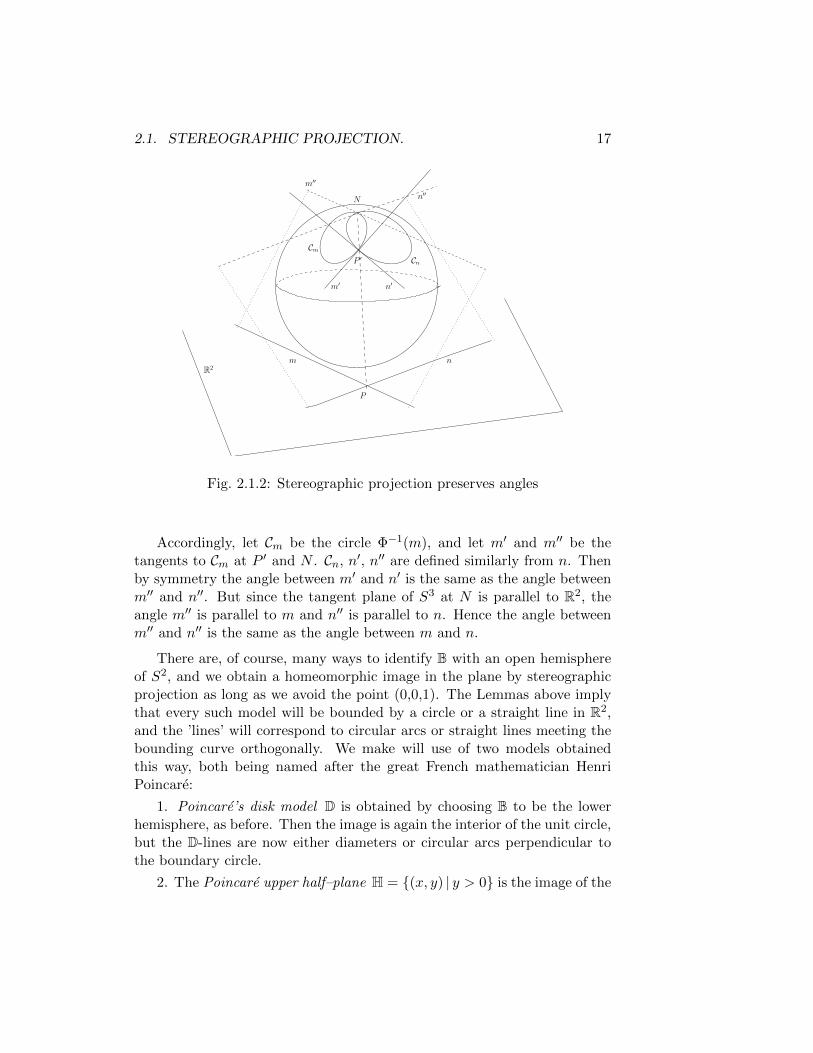
Figure 2.1.2 illustrates a geometric proof of Lemma 2.1.2. N is the“north pole”, P ′ is a point on S3 and P = Φ(P ). The lines m and n in R2
intersect in P . The crucial observation is that the image under Φ−1 of a lineis a circle — the intersection between S3 and the plane through the line andN . Moreover, the tangent line at a point Q of this circle is the intersectionbetween the plane and the tangent plane of S3 at Q.
2.1. STEREOGRAPHIC PROJECTION. 17
n
n′
P ′
m′′
m′
P
N
CmCn
m
n′′
R2
Fig. 2.1.2: Stereographic projection preserves angles
Accordingly, let Cm be the circle Φ−1(m), and let m′ and m′′ be thetangents to Cm at P ′ and N . Cn, n′, n′′ are defined similarly from n. Thenby symmetry the angle between m′ and n′ is the same as the angle betweenm′′ and n′′. But since the tangent plane of S3 at N is parallel to R2, theangle m′′ is parallel to m and n′′ is parallel to n. Hence the angle betweenm′′ and n′′ is the same as the angle between m and n.
There are, of course, many ways to identify B with an open hemisphereof S2, and we obtain a homeomorphic image in the plane by stereographicprojection as long as we avoid the point (0,0,1). The Lemmas above implythat every such model will be bounded by a circle or a straight line in R2,and the ’lines’ will correspond to circular arcs or straight lines meeting thebounding curve orthogonally. We make will use of two models obtainedthis way, both being named after the great French mathematician HenriPoincare:
1. Poincare’s disk model D is obtained by choosing B to be the lowerhemisphere, as before. Then the image is again the interior of the unit circle,but the D-lines are now either diameters or circular arcs perpendicular tothe boundary circle.
2. The Poincare upper half–plane H = (x, y) | y > 0 is the image of the

18 CHAPTER 2. HYPERBOLIC GEOMETRY
open hemisphere (x, y, z) ∈ S2 | y > 0. The H–lines are either semicircleswith center on the x-axis or straight lines parallel to the y-axis.
When we analyze these models we shall henceforth identify R2 withthe complex plane C and make use of the extra structure and tools wehave available there (complex multiplication, complex function theory, etc.).Thus, as sets we make the identifications D = z ∈ C | |z| < 1 and H =z ∈ C | Im z > 0.
D is the most symmetric of the two models and therefore often the onebest suited for geometric arguments. But we will see that H is better foranalyzing and describing the notion of congruence. Therefore this is wherewe begin our analysis.
Notation : In both models the hyperbolic lines have natural extensions tothe boundary curve. (The unit circle for D and the real line for H.) Theseextension points we refer to as endpoints of the hyperbolic lines, althoughthey are not themselves points on the lines. Analogously, we also say that∞ is an endpoint of a vertical H–line.
Exercises for 2.1
1. Derive the formulas for Φ and its inverse.
2. We can also define stereographic projection from (0, 0,−1) instead of(0, 0, 1). Let Φ− be the resulting map.
Determine the map Φ− Φ−1. (We identify R2 with C.)
3. If F is an identification between the two hemispheres we use in thedefinitions of H and D, the map ΦF Φ−1 will be a homeomorphismbetween the two models. Find a formula for such a homeomorphism.(Choose F as simple as possible.)
4. (a) Show that z 7→ z−1 : C−0 → C−0 corresponds to a rotationof S2 via stereographic projection.
(b) Which self–map of C − 0 does the antipodal map x 7→ −x onS2 − 0, 0,±1 correspond to?

2.2. CONGRUENCE IN H; MOBIUS TRANSFORMATIONS 19
2.2 Congruence in H; Mobius transformations
As noted before, we define congruence In Euclidean geometry as equivalenceunder the Euclidean group E(2) of “rigid movements”, generated by orthog-onal linear transformations x 7→ Ax and translations x 7→ x+b. This meansthat the congruence relation ∼= is defined by
Segments: AB ∼= A′B′ ⇐⇒ there is a g ∈ E(2) such that g(AB) = A′B′.Angles: ∠BAC ∼= ∠B′A′C ′ ⇐⇒ there is a g ∈ E(2) such that
g(−−→AB) =
−−→A′B′ and g(
−→AC) =
−−→A′C ′.
Observe that
Every element of E(2) maps straight lines to straight lines, andif A and A′ are points on the lines l and l′, there is a g ∈ E(2)such that g(l) = l′ and g(A) = A′.
We now wish to do something similar in the case of H. Motivated bythe Euclidean example, we will look for a group G of bijections of H to itselfsuch that
Every element of G maps H–lines to H–lines, and if A and A′ arepoints on the H-lines l and l′, there is a g ∈ G such that g(l) = l′
and g(A) = A′.
We will show that there exists such a group, consisting of so–calledMobius transformations preserving the upper half–plane.
From complex function theory we know that meromorphic functions withat most poles at∞ can be thought of as functions f : C→ C, where C is theextended complex plane or the Riemann sphere C ∪ ∞, with a topologysuch that stereographic projection extends to a homeomorphism Φ : S2 ≈ C.Lemma 2.1.1 says that Φ maps circles to curves in C that are either circlesin C or of the form l∪∞, where l is a (real) line in C. It is convenient notto have to distinguish between the two cases, so we call all of these curvesC–circles.
Similarly, we let R denote R ∪∞, considered as a subspace of C.
By Lemma 2.1.2 the angle between oriented such circles at an intersectionpoint in C is the same as between the corresponding circles on S2. Moreover,if they intersect in two points, the two angles will be the same. Hence we canalso define the angle at ∞ between two circles intersecting there — i. e. two
20 CHAPTER 2. HYPERBOLIC GEOMETRY
lines in C. If they intersect in a point P ∈ C, the angle of intersection at ∞is the same as the angle at P . If they are parallel, the angle of intersectionat ∞ is 0. With this definition, Φ is also angle preserving at ∞.
For a meromorphic function f : C→ C to be a homeomorphism, it musthave exactly one pole and one zero — hence it must have the form
f(z) =az + b
cz + d,
where a, b, c, d ∈ C. Solving the equation w = f(z) with respect to z we get
z = g(w) =−dw + b
cw − a,
and (formally) substituting back again:
f(g(w)) =(ad− bc)wad− bc
and g(f(z)) =(ad− bc)zad− bc
.
Therefore f is invertible with g as inverse if ad− bc 6= 0. If ad− bc = 0 theseexpressions have no meaning, but it is easy to see that in that case f(z) isconstant. Hence we have:
The function f(z) =az + b
cz + ddefines a homeomorphism of C if
and only if ad− bc 6= 0.
Such a function is called a fractional linear transformation — FLT forshort. Here are some crucial properties of FLT’s:
Lemma 2.2.1. (i) An FLT maps C–circles to C–circles.(ii) An FLT preserves angles between C–circles.
Proof. (i) Note that we may write the equations of both circles and straightlines in C as λ(x2 + y2) +αx+βy+ γ = 0, where λ, α, β, γ are real numbersand z = x + iy; λ = 0 for straight lines and λ 6= 0 for circles. Using thatx2 + y2 = zz, x = (z + z)/2 and y = (z − z)/2i = (z − z)i/2, we can writethe equation as
λzz + µz + µz + γ = 0 ,
where µ = (α − iβ)/2. Hence we need to show that if z satisfies such anequation and w = f(z) for an FLT f , then w satisfies a similar equation.
This can be checked by writing z = f−1(w) =aw + b
cw + dand substituting:
λaw + b
cw + d· aw + b
cw + d+ µ
aw + b
cw + d+ µ
aw + b
cw + d+ γ = 0 .

2.2. CONGRUENCE IN H; MOBIUS TRANSFORMATIONS 21
If we multiply this equation by (cw + d)(cw + d) and simplify, we end upwith an expression just like the one we want.
(ii) This is a consequence of a general fact in complex function theory.We say that a differentiable map is angle–preserving, or conformal, if itmaps two intersecting curves to curves meeting at the same angle. It thenfollows from the geometric interpretation of the derivative that a complexfunction is conformal in a neighborhood of any point where it is analyticwith nonzero derivative.
For a more direct argument in our case, see Exercise 3.
Remark 2.2.2. As in Lemma 2.1.2 it is not difficult to show that the sameresult is true for oriented angles (with a suitable notion of orientation thatalso applies to ∞ ∈ C), but we do not need that. An angle–preserving map(in the orientable sense) is called conformal, and it follows from the geometricinterpretation of the derivative that a complex function is conformal in aneighborhood of any point where it is analytic with nonzero derivative.
The oriented version of Lemma 2.1.2 says that stereographic projectionalso is conformal.
The word ’linear’ in FLT is related to the following remarkable observa-tion:
Let f(z) =az + b
cz + dand g(z) =
a′z + b′
c′z + d′. A little calculation gives
(f g)(z) = f(g(z)) =a g(z) + b
c g(z) + d=
(aa′ + bc′)z + (ab′ + bd′)
(ca′ + dc′)z + (cb′ + dd′).
This formula tells us two things. First, it means that the compositionof two FLT’s is a new FLT. We showed earlier that the inverse of an FLT isan FLT, and the identity map is trivially also an FLT. (z = 1z+0
0z+1 .) Hencethe set of fractional linear transformations forms a group under composi-tion. This group will be denoted Mob+(C) . (The “even complex Mobiustransformations”.)
Secondly, it is possible to calculate with FLT’s as with matrices: Evi-
dently the matrix
[a bc d
]determines f completely, and the condition ad−
bc 6= 0 simply means that this matrix is invertible. In the same way g
is determined by
[a′ b′
c′ d′
], and the calculation above shows that f g is
determined by the product matrix
[a bc d
]·[a′ b′
c′ d′
].

22 CHAPTER 2. HYPERBOLIC GEOMETRY
The set of invertible 2 × 2–matrices over C forms a group — the gen-eral linear group GL2(C) — and we have shown that there is a surjectivegroup homomorphism from GL2(C) onto Mob+(C) . This homomorphism
is not injective, since if k 6= 0, then
[a bc d
]and
[ka kbkc kd
]= k
[a bc d
]will
determine the same map. However, this is the only ambiguity (Exercise 4),and we get an isomorphism between the group Mob+(C) of fractional lineartransformations and the quotient group PGL2(C) = GL2(C)/D (the pro-jective linear group), where D = uI|u ∈ C − 0 and I is the identitymatrix.
(A more conceptual explanation of the connection between FLT’s andlinear algebra belongs to projective geometry — see Exercise 11).
The next Lemma and its Corollary tell us exactly what freedom we havein prescribing values of fractional linear transformations. In fact, it providesus with a method of constructing FLT’s with prescribed values.
Lemma 2.2.3. Given three distinct points z1, z2 and z3 in C. Then thereexists a uniquely determined FLT f such that f(z1) = 1, f(z2) = 0 andf(z3) =∞.
Proof. Existence : Suppose first that none of the zi’s is at∞. Then we define
f(z) =z − z2
z − z3· z1 − z3
z1 − z2.
In the three other cases:
if z1 =∞ : f(z) =z − z2
z − z3,
if z2 =∞ : f(z) =z1 − z3
z − z3,
if z3 =∞ : f(z) =z − z2
z1 − z2.
Uniqueness : Suppose g(z) has the same properties and consider the com-position h = g f−1. This is a new FLT with h(1) = 1, h(0) = 0 andh(∞) = ∞. The last condition implies that h must have the form h(z) =az + b, and the first two conditions then determine a = 1 og b = 0. Thus(g f−1)(z) = z for all z, hence f = g.
Definition 2.2.4. The element f(z) ∈ C depends on the four variables(z, z1, z2, z3) and is denoted [z, z1, z2, z3]. It is defined as an element of Cwhenever z1, z2 and z3 are distinct points of C and it has the followinggeometric interpretation:

2.2. CONGRUENCE IN H; MOBIUS TRANSFORMATIONS 23
If z2 and z3 span a Euclidean segment S, every point in S will divide itin two and we can compute the ratio between the lengths of the pieces. Ifwe do this for two points z and z1 in S, then |[z, z1, z2, z3]| is the quotientof the two ratios we obtain. Because of this, [z, z1, z2, z3] is traditionallycalled the cross–ratio of the four points, and it plays a very important rolein geometry. We shall meet it again later, and some of its properties aregiven below, in Proposition 2.2.10.
Corollary 2.2.5. Given two triples (z1, z2, z3) og (w1, w2, w3) of distinctpoints in C. Then there exists a unique FLT f such that f(zi) = wi, i =1, 2, 3. If all six points lie in R, then f may be expressed with real coefficients
— i. e. f(z) =az + b
cz + dwith a, b, c, d all real.
Proof. By Lemma 2.2.3 we can find unique FLT’s h and g such that h(z1) =1, h(z2) = 0, h(z3) = ∞, and g(w1) = 1, g(w2) = 0 g(w3) = ∞. Letf = g−1h. Then f(zi) = wi, i = 1, 2, 3.
Suppose also f ′ maps zi to wi. Then gf and gf ′ are both FLT’s as inLemma 2.2.3, and because of the uniqueness gf = gf ′. Consequently f = f ′.
The final assertion of the Corollary follows from the formulas in theproof of 2.2.3. They show that h and g have real coefficients, hence so doesf = g−1h.
Remark 2.2.6. The existence of such f means that the group Mob+(C) actstransitively on the set of such triples. The uniqueness says that if two frac-tional linear transformations have the same values at three points, then theyare equal. In particular, an FLT fixing three points is the identity map.
Note that f(z) is characterized by the equation
[f(z), w1, w2, w3] = [z, z1, z2, z3] .
Our next observation is that Mob+(C) also acts transitively on the set ofC–circles. The reason for this is that three distinct points in C determine aunique C–circle containing all of them.
Corollary 2.2.7. Given two circles C1 and C2 in C. Then there exists afractional linear transformation f such that f(C1) = C2.
Proof. Choose three distinct points (z1, z2, z3) on C1 and (w1, w2, w3) on C2,and let f be as in the Corollary above. Then f(C1) is a C–circle whichcontains w1, w2 and w3 — i. e. C2.

24 CHAPTER 2. HYPERBOLIC GEOMETRY
We now want to determine the fractional linear transformations f whichrestrict to homeomorphisms of the upper half–plane. Such an f is charac-terized by f(R) = R, and Im f(z) > 0 if Im z > 0. Here R = R ∪ ∞ ⊂ C.
Proposition 2.2.8. A fractional linear transformation restricts to a home-
omorphism of H if and only if it can be written on the form f(z) =az + b
cz + d,
where a, b, c, d are real and ad− bc = 1.
Such FLT’s map H–lines to H–lines.
Proof. Corollary 2.2.5 says that if f(z) =az + b
cz + drestricts to a homeomor-
phism of H, then a, b, c, d can be chosen to be real, since f(R) = R. Con-versely, f(R) = R if a, b, c, d are real.
A short calculation gives
f(z) =(az + b)(cz + d)
(cz + d)(cz + d)
=ac|z|2 + (ad+ bc)Re z + bd
|cz + d|2+
(ad− bc)Im z
|cz + d|2i . (2.2.1)
It follows that f preserves the upper half–plane if and only if ad − bc > 0.Hence, if we multiply a, b, c and d by 1/
√ad− bc, f is as asserted.
The last claim follows immediately from the fact that fractional lineartransformations preserve C–circles and angles between them. Every H–linedetermines a C–circle which meets R orthogonally, and since f preservesangles and f(R) = R, the images of these circles will also meet R orthogo-nally.
The fractional linear transformations restricting to homeomorphisms ofH form a subgroup of of Mob+(C) denoted Mob+(H).It can also be describedusing matrices, as follows:
Let SL2(R) be the special linear group — the group of real 2×2–matriceswith determinant 1. The only multiples of the identity matrix in SL2(R) are±I, hence, arguing as before, we get an isomorphism between Mob+(H) andthe quotient group PSL2(R) = SL2(R)/(±I).
Mob+(C) does not contain all circle–preserving homeomorphisms of C.Complex conjugation is also circle–preserving but not even complex analytic.(Define ∞ = ∞.) We define the group of complex Mobius transformations,Mob(C),to be the group of homeomorphisms of C generated by the fractionallinear transformations and complex conjugation.

2.2. CONGRUENCE IN H; MOBIUS TRANSFORMATIONS 25
Proposition 2.2.9. (1) Every complex Mobius transformation can be writ-ten on exactly one of the forms
f(z) =az + b
cz + dor f(z) =
az + b
cz + d, where a, b, c, d ∈ C and ad− bc = 1 .
(2) The complex Mobius transformations preserving H can be written eitheras
(i) f(z)=az + b
cz + d, where a, b, c, d ∈ R and ad− bc = 1 , or as
(ii) f(z)=az + b
cz + d, where a, b, c, d ∈ R og ad− bc = −1 .
Proof. (1) Let S be the subset of the set of homeomorphisms of C givenby such expressions. Clearly S ⊆ Mob(C) , and S contains Mob+(C) andcomplex conjugation. Therefore it suffices to check that S is closed undercomposition and taking inverses, and this is an easy calculation. Moreover,the second expression is not even complex differentiable, hence no functioncan be written both ways.
To obtain determinant 1 we divide numerator and denominator by asquare root of ad− bc.
(2) f(z) can be written in one of the two types in (1). In the first case,
the result is given in Proposition 2.2.8. If f(z) =az + b
cz + d, then g(z) = −f(z)
can be written as in (i). But then f(z) = −g(z) automatically has the formgiven in (ii).
The representations in Proposition 2.2.9 is not unique, but it follows fromthe result in Exercise 4 that it is unique up to multiplication of (a, b, c, d)by ±1.
Let Mob(H) be the group of Mobius transformations restricting to home-omorphisms of H. We have shown that every element in Mob(H) can bewritten as one of the two types in (2) of Proposition 2.2.9, and thereforewe call these elements the real Mobius transformations. Note that complexconjugation, i. e. reflection in the real axis, is not in Mob(H), but f(z) = −z,reflection in the imaginary axis, is. Mob(H) is generated by this reflectionand Mob+(H) .
We use the notation Mob−(H) for the elements in Mob(H) of type (ii).These do not form a subgroup, but Mob(H) is the disjoint union of Mob+(H)and Mob−(H) . In fact, Mob+(H)⊂Mob(H) is a normal subgroup of indextwo, and Mob−(H) is the coset containing −z.

26 CHAPTER 2. HYPERBOLIC GEOMETRY
Mob(H) is the group we shall use to define congruence in H, but beforewe show that Hilbert’s axioms hold, we will analyze the elements in Mob(H)further (next section) and show that they can be classified into a few verysimple standard types.
We end this section with some properties satisfied by the cross ratio.
Proposition 2.2.10. Assume that z, z1, z2 and z3 are four distinct pointsin C, and let ρ = [z, z1, z2, z3]. Then
(i) [z1, z, z2, z3] = [z, z1, z3, z2] =1
ρ, and [z, z2, z1, z3] = 1− ρ.
(ii) z, z1, z2 and z3 all lie on the same C–circle if and only if the cross–ratio[z, z1, z2, z3] is real.
(iii) [g(z), g(z1), g(z2), g(z3)] = [z, z1, z2, z3] if g is a fractional linear trans-formation.
Proof. (i) Recall that the mapping w 7→ f(w) = [w, z1, z2, z3] is the frac-tional linear transformation which is uniquely determined by its values1, 0 and ∞ at the points z1, z2 and z3, respectively. Then the identities
[w, z1, z3, z2] =1
f(w)and [w, z2, z1, z3] = 1 − f(w) follow easily by inspec-
tion. Setting w = z proves two of the identities.Note that since f(z2) = 0 and f(z3) = ∞, ρ is not 0 or ∞. Therefore
g(w) =1
ρf(w) defines a new fractional linear transformation. But g(z) =
1, g(z2) = 0 and g(z3) =∞ — hence g(w) = [w, z, z2, z3]. Consequently,
[z1, z, z2, z3] = g(z1) =1
ρ[z1, z1, z2, z3] =
1
ρ.
(ii) Let C be the unique C–circle containing the three points z1, z2 andz3. Then f(C) must be the unique C–circle containing 1, 0 and ∞ — i. e. R.Likewise, f−1(R) = C. Thus z ∈ C if and only if f(z) ∈ R. But since z 6= z3,f(z) ∈ R means f(z) ∈ R.
(iii) Let h(w) = [g(w), g(z1), g(z2), g(z3)]. This is a composition of twoFLT’s — hence h is also an FLT. By inspection, h(zj) = [zj , z1, z2, z3] forj = 1, 2, 3. Therefore h(w) = [w, z1, z2, z3] for all w, by uniqueness.
Remark 2.2.11. (1) The three transpositions (1,2), (2,3) and (3,4) generatethe whole group S4 — the group of permutations of four letters. Hence (i)

2.2. CONGRUENCE IN H; MOBIUS TRANSFORMATIONS 27
can be used to determine the cross ratio of any permutation of the pointsz, z1, z2 and z3. For examples, see Exercise 8.
It follows that [z, z1, z2, z3] can be defined as long as three of the pointsz, z1, z2 and z3 are distinct, and it can be considered as a fractional lineartransformation in each of the variables separately. This observation will beused repeatedly later without any further comment.
(2) The identity in (iii) is not valid for all Mobius transformations g. Forexample, if g(z) = z, then [g(z), g(z1), g(z2), g(z3)] = [z, z1, z2, z3]. (Exercise9.)
Exercises for 2.2
1. Discuss what conditions λ, µ, γ must satisfy for λzz+µz+ µz+γ = 0to define an H–line.
2. Let the circle C be given by the equation |z− z0| = r, and let f be thefunction f(z) = 1/z. When is f(C) a straight line ∪∞?
3. Show that any FLT can be written as a composition of maps of thefollowing three simple types:
(i) Translations z 7→ z + b, b ∈ C,
(ii) Linear maps z 7→ kz, k ∈ C− 0,
(iii) Taking inverse z 7→ 1
z.
Use this to give another proof of Lemma 2.2.1. (Hint: You may findExercise 2.1.4a useful.)
4. Assume ad − bc 6= 0. Show thataz + b
cz + d=a′z + b′
c′z + d′for every z if and
only if there exists a k 6= 0 such that
[a′ b′
c′ d′
]= k
[a bc d
].
5. Use the method of Corollary 2.2.5 to find explicit fractional lineartransformations mapping H onto D and vice versa. (Compare withExercise 2.1.3.)
6. Describe all the elements in Mob(H) that map the imaginary axis toitself.
28 CHAPTER 2. HYPERBOLIC GEOMETRY
7. (a) Show that Mob(H) acts transitively on the set of all triples of dis-tinct points in R. Deduce that Mob(H) acts transitively on the set ofpairs of lines in H with one common endpoint.
(b) Let ` and `′ be two H-lines with endpoints z, w and z′, w′, resp.,and let p ∈ ` and p′ ∈ `′ be given points on the lines. Show thatthere is a unique f ∈ Mob+(H) such that f(z) = z′, f(w) = w′, andf(p) = p′.
(c) Show that Mob(H) does not act transitively on the set of pairs ofdistinct points in H.
8. Using Remark 2.2.11, show that if [z1, z2, z3, z4] = ρ, then
[z3, z4, z1, z2] = ρ and [z3, z2, z1, z4] =ρ
1− ρ.
9. Show that [g(z), g(z1), g(z2), g(z3)] = [z, z1, z2, z3] for all g ∈Mob(C) .
10. Give a geometric explanation for Prop. 2.2.10(ii).
Suppose z1, z2, z3 ∈ R and consider the function g(z) = [z, z1, z2, z3].Discuss when we have g ∈Mob+(H) .
11. Show that Mob(H) is isomorphic to the group PGL2(R) = GL2(R)/D,where D = uI|u ∈ R− 0.
12. Let CP 1 = (C2 − 0)/∼, where ∼ is the equivalence relation whichidentifies v and λv, for all v ∈ C2 − 0 and λ ∈ C − 0. (CP 1 iscalled the complex projective line.)
Show that multiplication by a matrix in GL2(C) induces a bijectionof CP 1 with itself.
Verify that (z1, z2) 7→ z1/z2 defines a bijection CP 1 ≈ C, and show
that via this bijection, multiplication with the matrix
[a bc d
]corre-
sponds to the fractional linear transformationaz + b
cz + d.
Why does it now follow immediately that this correspondence is agroup homomorphism GL2(C)→Mob+(C) ?

2.3. CLASSIFICATION OF REAL MOBIUS TRANSFORMATIONS 29
2.3 Classification of real Mobius transformations
Since the Mobius transformations play such an important role in the theory,we would like to know as much as possible about them, both geometricallyand algebraically. The results of this section can be interpreted in bothdirections. Geometrically we show that up to coordinate shifts, Mobiustransformations can be given one of three possible “normal forms”, fromwhich it is easy to get a good picture of how they act on H. Algebraicallythis translates into a classification into conjugacy classes in Mob(H) .
Since Mob(H) is isomorphic to a matrix group, this classification couldbe done completely with tools from linear algebra. What we will do isequivalent to this, but interpreted in our geometric language.
The key to the classification of matrices is the study of eigenvectors, andit is not difficult, using Exercise 2.2.12, to see that in Mob(C) this corre-sponds to analyzing the fixpoints of the transformations, i. e. the solutionsin C of the equation z = f(z). By a “change of coordinates” we reduce toa situation where the fixpoint set is particularly nice. Then we can moreeasily read off the properties of f .
Let us first consider the subgroup Mob+(H)⊂Mob(H). We have seen
that an element here can be written f(z) =az + b
cz + d, where ad− bc = 1. We
assume from now on that f has this form and is not the identity.Observe that as a map C→ C, f has ∞ as fixpoint if and only if c = 0.
Then f(z) = a2z + ab. If also a = d, or a2 = 1, this is the only fixpoint —otherwise we have one more, namely z = −b/(a− d) = ab/(1− a2), which isa real number. In other words, if c = 0 we have either one or two fixpoints,and they lie in R.
If c 6= 0, the equation z =az + b
cz + dis equivalent to the equation
cz2 − (a− d)z − b = 0 ,
with roots
z =a− d±
√(a− d)2 + 4bc
2c.
Using that ad− bc = 1, we can simplify the square root and write
z =a− d±
√(a+ d)2 − 4
2c.
We see that we should distinguish between three cases:

30 CHAPTER 2. HYPERBOLIC GEOMETRY
• (a+ d)2 = 4: Exactly one real root
• (a+ d)2 > 4: Two real roots
• (a+ d)2 < 4: Two complex roots
The number a + d is the trace of the matrix
[a bc d
], and it is invariant
under conjugation by elements of GL2(C). The trace of −[a bc d
]is −(a+d),
so it follows that the number
τ(f) = (a+ d)2
is invariant under conjugation of f by elements inMob+(H) . In fact, it is alsoinvariant under conjugation by z 7→ −z, hence invariant under conjugationby every element of Mob(H) .
Note that if c = 0, then ad = 1 and (a + d)2 = (a − d)2 + 4 ≥ 4, withequality if and only if a = d. Taking into account the discussion above of thecase c = 0, we can distinguish between the following three cases, regardlessof the value of c:
• Exactly one fixpoint in R, when τ(f) = 4. We then say that f is ofparabolic type.
• Two fixpoints in R, when τ(f) > 4. f is of hyperbolic type.
• Two fixpoints in C, when τ(f) < 4. f is of elliptic type.
Let us consider more closely each of the three cases:
Case (1) : One fixpoint in R; f is of parabolic type.
If the fixpoint is at ∞, we must have c = 0, and f(z) has the formf(z) = z + β, i. e. f is a translation parallel to the x–axis.
If the fixpoint is q ∈ R, we can find an h ∈Mob+(H) mapping q to ∞.(Choose e. g. h(z) = −1/(z − q).) Then the composition g = h f h−1
is also an element of Mob+(H), and g has ∞ as unique fixpoint. Hence, asabove, g has the form
g(z) = z + γ
for a real number γ.

2.3. CLASSIFICATION OF REAL MOBIUS TRANSFORMATIONS 31
In fact, we can do even better than this: γ 6= 0, so we can conjugate g
by k(z) =z
|γ|:
k g k−1(z) = z ± 1.
Hence any parabolic transformation is conjugate to a translation of the formz + 1 or z − 1. These two translations are conjugate in Mob(H) , but not inMob+(H) . (See Exercise 5.)
We think of such a conjugation as a change of coordinates: writingf = h−1 g h, we see that f(z) is obtained by first moving z to h(z), thenapplying g and finally moving back again by h−1.
g fixes the point ∞ and translates horizontally all straight lines orthog-onal to the real axis, i. e. H–lines ending in ∞. Since h and h−1 both mapH–lines to H–lines, we see that f must map H–lines ending in q to H–linesof the same type.
Figure 2.3.1 illustrates this in more detail. If g translates the verticallines horizontally, it must also preserve the horizontal lines (dashed lines inthe left figure). Mapped back by h−1 these become circles, but these circlesare now tangent to the x–axis, as in the figure to the right. It follows thatf also must preserve such circles.
Remark 2.3.1. Such (Euclidean) circles, tangent to R at a point p, are calledhorocircles at p. They can also be characterized by the property that theyare orthogonal to all hyperbolic lines ending at the point of tangency (SeeExercise 3). Another characterization is discussed in Exercise 2.7.5.
g(w) w
z
f(z)
l
f(l)
g(m) m=h(l)
q
sh(s)
h
gf
Fig. 2.3.1: Parabolic Mobius transformation
Case (2) : f is of hyperbolic type, i. e. τ(f) = (a + d)2 > 4 and f has twofixpoints in R.

32 CHAPTER 2. HYPERBOLIC GEOMETRY
Let h ∈Mob+(H) be a real FLT mapping the two fixpoints to 0 and ∞.Then g = h f h−1 ∈Mob+(H) has 0 and ∞ as fixpoints. It also mapsthe imaginary axis to an H–line l, But since the end points are fixed, theend points of l are again 0 and ∞, so l must also be the imaginary axis. Inparticular there is a positive real number η such that g(i) = ηi, and sincewe know that g is uniquely determined by the values at the three points 0,i and ∞, we must have
g(z) = ηz
for all z. Thus, up to a change of coordinates, f is just multiplication by areal number.
Write η = λ2, such that g(z) =λz
λ−1, where we also may assume λ > 0.
Since we must have τ(g) = τ(f), λ satisfies the equation
λ+1
λ= |a+ d| .
This equation has two roots λ and 1/λ, and the corresponding functionsλ2z and z/λ2 are conjugate by the transformation z 7→ −1/z — hence theyare both realized by different choices of h. It follows that if we also chooseη > 1, g(z) = ηz is uniquely determined. Moreover, this g(z) is invariantunder conjugation by −z. Therefore there is a one–one correspondencebetween conjugacy classes of hyperbolic elements and real numbers > 1, inboth Mob+(H) and Mob(H) .
Hyperbolic transformations behave as in figure 2.3.2. g preserves straightlines through 0, and these are mapped by h−1 to circular arcs or straightlines through the fixpoints of f , but the image of the imaginary axis is theonly such curve meeting the x–axis orthogonally. Hence this is an H–linebetween the two fixpoints of f , and it is mapped to itself by f . We call thisH–line the axis of f .
An element of Mob+(H) of hyperbolic type with axis l is often called a“translation along l”.
Case (3) : The final case is when we have two complex fixpoints — the ellipticcase, when τ(f) < 4.
Since the two fixpoints are the roots of a real, quadratic equation, theyare complex conjugate. In particular, there is exactly one in the upper half–
plane and none in R. Let p be the fixpoint in H and set h(z) =z − Re p
Im p,
such that h ∈Mob+(H) and h(p) = i. This time g = h f h−1 will be areal fractional linear transformation fixing i.
2.3. CLASSIFICATION OF REAL MOBIUS TRANSFORMATIONS 33
g
fh
p0=h(p)
zf(z)
w
g(w)
w=h(z)
Fig. 2.3.2: Hyperbolic Mobius transformation
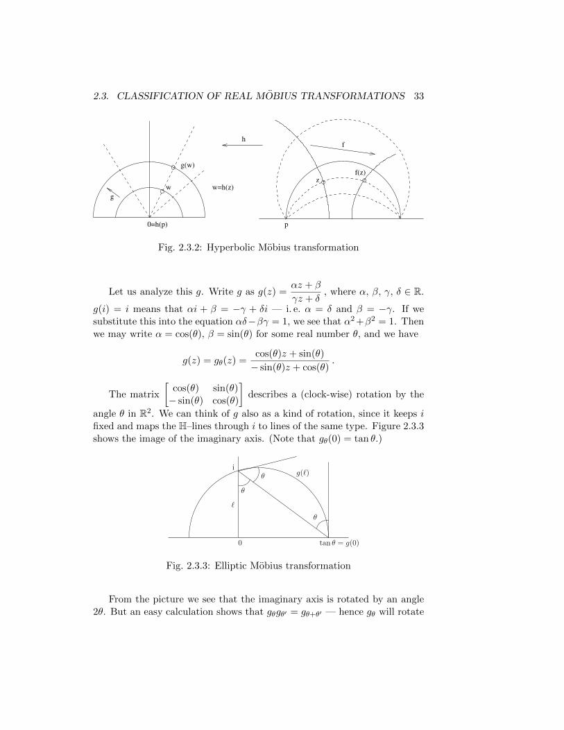
Let us analyze this g. Write g as g(z) =αz + β
γz + δ, where α, β, γ, δ ∈ R.
g(i) = i means that αi + β = −γ + δi — i. e. α = δ and β = −γ. If wesubstitute this into the equation αδ−βγ = 1, we see that α2 +β2 = 1. Thenwe may write α = cos(θ), β = sin(θ) for some real number θ, and we have
g(z) = gθ(z) =cos(θ)z + sin(θ)
− sin(θ)z + cos(θ).
The matrix
[cos(θ) sin(θ)− sin(θ) cos(θ)
]describes a (clock-wise) rotation by the
angle θ in R2. We can think of g also as a kind of rotation, since it keeps ifixed and maps the H–lines through i to lines of the same type. Figure 2.3.3shows the image of the imaginary axis. (Note that gθ(0) = tan θ.)
0
g(`)
`
tan θ = g(0)
θ
iθ
θ
Fig. 2.3.3: Elliptic Mobius transformation
From the picture we see that the imaginary axis is rotated by an angle2θ. But an easy calculation shows that gθgθ′ = gθ+θ′ — hence gθ will rotate
34 CHAPTER 2. HYPERBOLIC GEOMETRY
any H–line through i by an angle 2θ. In particular, gπ =id, and gθ+π = gθ.Later, after we have introduced Poincare’s disk–model, the analogy with
Euclidean rotations will become even clearer. See also Exercise 6.
If gθ is conjugate to gθ′ in Mob+(H) , then gθ = gθ′ . The reason for this isthat if h−1gθh has i as fixpoint, then gθ has h(i) as fixpoint — hence h(i) = i.But then h = gφ for some φ; thus gθ and h commute. It follows that there isa one–one correspondence between conjugacy classes in Mob+(H) of ellipticelements and angles θ ∈ (0, π).
On the other hand, if h(z) = −z, then h−1gθh = g−θ = gπ−θ, so theconjugacy classes inMob(H) are in one–one correspondence with θ ∈ (0, π/2].
Let us sum up what we have done so far:
Proposition 2.3.2. Suppose f(z) =az + b
cz + d, where a, b, c, d ∈ R and ad−
bc = 1, and let τ(f) = (a + d)2. Assume that f is not the identity map.Then, as an element of Mob+(H) , f is of
• Parabolic type, conjugate to z 7→ z + 1 or z − 1, if τ(f) = 4,
• Hyperbolic type, conjugate to exactly one z 7→ ηz with η > 1, if τ(f) >4,
• Elliptic type, conjugate to a unique z 7→ gθ(z) =cos(θ)z + sin(θ)
− sin(θ)z + cos(θ)with θ ∈ (0, π) , if τ(f) < 4.
In Mob(H) the only differences are that there is only one conjugacy classof elements of parabolic type (see Exercise 5), and gθ is conjugate to gπ−θ.
We say that an element of Mob+(H) is given on normal form if it iswritten as a conjugate of one of these standard representatives.
We now move on to Mob−(H) and consider a transformation of the form
f(z) =az + b
cz + d, where a, b, c, d ∈ R and ad− bc = −1.
Again we will look for fixpoints of f(z). As before, z = ∞ is a fixpointif and only if c = 0. If z 6= ∞, the equation f(z) = z is now equivalent toc|z|2 + dz − az − b = 0, or
c(x2 + y2)− (a− d)x− b = 0, (2.3.1)
(a+ d)y = 0. (2.3.2)
We consider the two cases a+ d = 0 and a+ d 6= 0 separately.

2.3. CLASSIFICATION OF REAL MOBIUS TRANSFORMATIONS 35
First, let a+ d = 0. In this case equation (2.3.2) is trivially satisfied, sowe have only one equation (2.3.1). This describes an H–line : the vertical
line x =b
d− awhen c = 0 and the semi–circle with center (a/c, 0) and
radius 1/|c| if c 6= 0. (Note that a 6= d if c = 0, since then ad = −1.)Hence f fixes an entire H–line and interchanges the two components of itscomplement in H. More precisely, by a suitable conjugation as above, wemay assume that the fixed H–line is the imaginary axis. Then c = b = 0and a = −d = ±1 — hence f(z) = −z. Thus all such transformations areconjugate to the horizontal reflection in the imaginary axis.
If the fixpoint set is another vertical line l, we can choose h to be ahorizontal translation. Hence f must be horizontal reflection in l.
If c 6= 0 we can also write
f(z) =a
c+
1/c
cz + d=a
c+
1/c2
z − a/c. (2.3.3)
This has the general form
g(z) = m+r2
z −m= m+ r2 z −m
|z −m|2.
If C is the circle (completion of an H-line) with center m and radius r,g(z) maps points outside C to points inside and vice versa, and it leaves thecircle itself fixed. More precisely, we see that g(z) lies on the (Euclidean)ray from m through z, and such that the product |g(z)−m||z−m| is equalto r2. This is a very important geometric construction called “inversion inthe circle C”.
By analogy we will also call the horizontal reflection in a vertical line l“inversion in l”. Thus inversions in H-lines are precisely the transformationsin Mob−(H) such that a + d = 0, and all inversions are conjugate. Thereare two particularly simple representatives for this conjugacy class: the hor-izontal reflection z 7→ −z and the map z 7→ 1/z, which is inversion in thecircle |z| = 1. Either of these could be considered a “normal form” of suchmaps, but note that they all are inversions a priori, not only after a changeof coordinates.
Next, assume a+ d 6= 0. Then y = 0 by (2.3.2), so there are no fixpointsin H. In equation (2.3.1) we distinguish between the cases c = 0 and c 6= 0.
If c = 0, we get x = b/(d− a), but then we also have the fixpoint (in C)z =∞, so f must map the vertical line x = b/(d−a) to itself. (But withoutfixpoints.) Note that we cannot have a = d, since ad = −1.

36 CHAPTER 2. HYPERBOLIC GEOMETRY
If c 6= 0, (2.3.1) has two solutions x =a− d±
√(a+ d)2 + 4
2cin R.
Hence f(z) has two fixpoints on the real axis, and f must map the H–linewith these two points as endpoints to itself.
Thus, in both cases f preserves an H–line `, fixing the endpoints, andconjugating with a transformation mapping ` to the imaginary axis, weobtain a function of the form k(z) = −λ2z — a composition of the reflection(inversion) in the y–axis and a hyperbolic transformation with the sameaxis.
Note that as λ2(−z) = −(λ2z), these two transformations commute.Conjugating back, we see that we have written f as a composition of twocommuting transformations — a hyperbolic transformation h and an inver-sion g in the axis of h. Observe also that if λ2 6= 1, the imaginary axis isthe only H–line mapped to itself by k(z) = −λ2z. It follows that the line `above is the only line such that f(`) = `. This is used in the proof of thefollowing proposition:
Proposition 2.3.3. Let f ∈Mob−(H) have the form f(z) =az + b
cz + d, where
a, b, c, d ∈ R and ad− bc = −1.
• If a+ d = 0, then f an inversion, conjugate to reflection in the imag-inary axis.
• If a + d 6= 0, f can be written f = gh, where g is an inversion and gand h commute. Moreover, this decomposition is unique and h is ofhyperbolic type and with axis equal to the line of inversion of g.
Proof. It only remains to prove the uniqueness statement. So, suppose f =gh = hg, where g is inversion in a line `. If z ∈ ` we have
g(h(z)) = h(g(z) = h(z) ,
i. e. h(z) is a fixpoint for g. Hence h(z) ∈ `. It follows that
f(`) = h(g(`)) = h(`) = ` .
By as we just observed, this determines `, hence also g. It is now clearthat g and h are uniquely determined as the two transformations constructedabove.
It is worth pointing out that if we do not require that the componentscommute, there are many ways of decomposing an element of Mob−(H) into

2.3. CLASSIFICATION OF REAL MOBIUS TRANSFORMATIONS 37
a product of an inversion and an element of Mob+(H) . Trivial such decom-positions are given by the formulas
az + b
cz + d=
(−a)(−z) + b
(−c)(−z) + d= −
((−a)z + (−b)
cz + d
).
More interesting, perhaps; if c 6= 0, we can generalize (2.3.3) and write(using ad− bc = −1):
az + b
cz + d=a
c+
1/c
cz + d=a+ d
c+
(−dc
+1
c2
z − (−d/c)|z − (−d/c)|2
). (2.3.4)
This is a composition of an inversion and a parabolic transformation. Formore on decompositions of Mobius transformations, see exercises 9 and 10.
Note the following, which is implicit in what we have done:
• An element in Mob−(H) is an inversion if and only if its trace a+ d is0. (This condition is independent of whether we have normalized thecoefficients or not.)
• An element in Mob−(H) is an inversion if and only if it has a fixpointin H.
• An inversion in an H–line l is characterized, as an element of Mob(H) ,by having all of l as fixpoint set.
Exercises for 2.3
1. Classify the following maps and write them explicitly as conjugates ofmappings on normal form.
4z − 3
2z − 1, − 1
z − 1,
z
z + 1.
2. Discuss the classification of Mobius transformations in terms of matrixrepresentations, without assuming determinant 1.
3. Show geometrically that the horocircles at a point p ∈ R are orthogonalto all H-lines with p as one endpoint.

38 CHAPTER 2. HYPERBOLIC GEOMETRY
4. Explain what a hyperbolic transformation f does to the horocircles atthe endpoints of the axis of f , and also to the other H–lines sharingthe same endpoint.
5. Show that all parabolic transformations are conjugate in Mob(H) .Show that the translations z 7→ z + 1 and z 7→ z − 1 are not con-jugate in Mob+(H) .
6. Fix a z in H, z 6= i. Show that as θ varies, the points gθ(z) all lie onthe same circle in C.
(Hint: if cos θ 6= 0,write gθ(z) =tan θ + z
− tan θ z + 1, and think of this as a
function of tan θ.)
7. Assume h1 and h2 are two nontrivial elements of Mob+(H) satsifyingh1h2 = h2h1. Show that they have the same fixpoints, hence are alsoof the same type.
8. Show that an inversion in a circle C ⊂ C, considered as a map on Cminus the center of C, has the following properties:
(a) It maps straight lines outside C to circles inside C and throughits center.
(b) Circles intersecting C orthogonally are mapped to themselves.
(These are important results about inversions that are usually provedby geometric arguments. Her they should follow quite easily from whatwe now know about Mobius transformations.) .
9. Show that every element in Mob+(H) may be written as the composi-tion of two inversions.
10. Show that Mob(H) is generated by inversions, and show that Mob+(H)(Mob−(H) ) consists of those elements that can be written as a com-position of an even (odd) number of inversions.

2.4. HILBERT’S AXIOMS AND CONGRUENCE IN H 39
2.4 Hilbert’s axioms and congruence in H
We are now ready to prove that the upper half-plane provides a model forthe hyperbolic plane satisfying the rest of Hilbert’s axioms, with congruencebased on the action of Mob(H) .
Recall that, using a combination of orthogonal and stereographic pro-jections, we have identified the open unit disk K ⊂ R2 with the upperhalf–plane H ⊂ C, such that chords in K correspond to what we have calledH-lines — vertical lines or semicircles with center on the real axis in C. Kinherits incidence and betweenness relations from R2, hence we obtain cor-responding relations in H. Automatically all of Hilbert’s axioms I1–3 andB1–4 for these relations hold, as does Dedekind’s axiom. In this section weintroduce a congruence relation and show that it satisfies Hilbert’s axiomsC1–6. Since the parallel axiom has been replaced by the hyperbolic axiom,we will then have completed the construction of a hyperbolic geometry.
Remark 2.4.1. Betweenness for points on a line in the Euclidean plane canbe formulated via homeomorphisms between the line and R or intervals inR, hence the same is true for H-lines, if we use the subspace topology fromC. On R the easiest definition is:
a ∗ b ∗ c ⇐⇒ a < b < c or a > b > c .
(Equivalently: (a− b)(b− c) > 0.) The simplest such homeomorphisms areprojections to the imaginary axis from the vertical lines and to the real axisfrom the half–circles. It follows that betweenness for points on an H–line `can be characterized by
• x ∗ y ∗ z ⇐⇒ Imx ∗ Im y ∗ Im z if ` is vertical,
• x ∗ y ∗ z ⇐⇒ Rex ∗ Re y ∗ Re z otherwise.
Before we go on, we need a more precise notation for lines, rays etc.If z1, z2 are two points of H, we write ←−→z1z2 for the uniquely determinedhyperbolic line containing them, −−→z1z2 for the ray from z1 containing z2 and[z1, z2] for the segment between z1 and z2 — i. e. [z1, z2] = −−→z1z2 ∩ −−→z2z1.An H–line l is uniquely determined by its endpoints p and q in R, andtherefore we will also write l = (p, q). With this notation, the identity←−→z1z2 = (p, q) will tell us that the uniquely determined H–line containing z1
and z2 has endpoints p and q. Similarly, we may also write [z1, q) = −→z1q =−−→z1z2, expressing that q is the endpoint of the ray −−→z1z2.

40 CHAPTER 2. HYPERBOLIC GEOMETRY
We say that z1 is the vertex and q the endpoint of the ray [z, q). An angleis then an unordered pair of rays with the same vertex, where the two raysdo not lie on the same line. We use the notation ∠uzv for the unorderedpair −→zu,−→zv, where z ∈ H and u, v are either in H or in R.
Recall that we have defined the two sides of a line l by saying that twopoints z1 and z2 are on the same side of l if [z1, z2] ∩ l = ∅. (Page 4 andexercise 1.1.4.) If r is the inversion in l, clearly [z, r(z)] ∩ l 6= ∅. Hence rinterchanges the two sides of l.
The congruence relation in H is now defined as follows:
Congruence of segments: [z1, z2] ∼= [w1, w2] ⇐⇒ g([z1, z2]) = [w1, w2]
for some g ∈Mob(H) .
Congruence of angles: ∠uzv ∼= ∠u′z′v′ ⇐⇒ g(−→zu) =−−→z′u′ and
g(−→zv) =−→z′v′ for some g ∈Mob(H) . (Notation: g(∠uzv) = ∠u′z′v′.)
The existence parts of the congruence statements say that there areenough Mobius transformations to move angles and segments freely aroundin H, whereas the uniqueness means that there are not too many such trans-formations. The technical results we need are contained in the followingLemmas:
Lemma 2.4.2. Suppose zj lies on an H–line lj, with endpoints pj and qj,for j = 1, 2. Then there is a uniquely determined f ∈Mob+(H) such thatf(p1) = p2, f(q1) = q2 and f(z1) = z2 — hence also f(l1) = l2.
In particular we have, for example, f([z1, q1)) = [z2, q2). But since a raydetermines the line containing it, we get
Corollary 2.4.3. Mob+(H) acts transitively on the set of all rays: In fact,given two rays σ1 and σ2 with vertices z1 and z2, there is a unique f ∈Mob+(H) such that f(z1) = z2 and f(σ1) = σ2.
Lemma 2.4.4. (i) An element in Mob+(H) is completely determined by itsvalues at two points in H.
(ii) Suppose the segments [z1, z2] and [w1, w2] are congruent. Then thereis a uniquely determined f ∈Mob+(H) such that f(z1) = w1 and f(z2) = w2.
Lemma 2.4.5. Given two rays σ1 and σ2 with a common vertex z0. Thenthere is a unique inversion g such that g(z0) = z0, g(σ1) = σ2 and g(σ2) =σ1.

2.4. HILBERT’S AXIOMS AND CONGRUENCE IN H 41
Proof of Lemma 2.4.2. This is Exercise 2.2.7b, but, for completeness, hereis a proof:
By Corollary 2.2.5 there exists a unique f ∈ Mob+(C) with the rightproperties, and all we have to prove is that it lies in Mob+(H) . Let Ci, i = 1, 2be the C-circle containing li (and determined by pi, qi and zi). Then wemust have f(C1) = C2, and f(R) is a C-circle meeting C2 in p2 and q2 atright angles. Hence f(R) = R, and f ∈Mob(H) . (Again by Corollary 2.2.5.)But since f(z1) = z2, we must have f ∈Mob+(H) .
Proof of Lemma 2.4.4. (i) Two points in H determine a unique line l, andthe endpoints of l must map to the endpoints of f(l), in such a way thatbetweenness relations are preserved. Hence the values of f at four points aredetermined, and the uniqueness follows from uniqueness in Corollary 2.2.5.
(ii) Assume that g([z1, z2]) = [w1, w2] for some g ∈Mob(H). If g ∈Mob−(H), we replace g by k g, where k is the inversion in the H–line←−→w1w2.Therefore we may assume that g ∈Mob+(H).
The problem is that we might have g(z1) = w2 and g(z2) = w1. If so,choose an h ∈Mob+(H) such that h(←−→w1w2) is the imaginary axis, and writeh(w1) = ω1i, h(w2) = ω2i. If we define k(z) = −ω1ω2/z, we see that kinterchanges ω1i and ω2i. Then h−1kh will interchange w1 og w2, and welet f = h−1khg.
Proof of Lemma 2.4.5. It follows easily from Lemma 2.4.2 that we can findan h ∈Mob+(H) mapping σ1 to σ2. (h has z0 as fixpoint and must necessarilybe elliptic.) Let r be inversion in the line containing σ1 and define g = hr.Then g ∈Mob−(H) and has a fixpoint z0 ∈ H, hence is also an inversion(Remark at the end of 2.2.) Clearly g(σ1) = h(σ1) = σ2, and then g(σ2) =g2(σ1) = σ1.
Uniqueness: Suppose g′ is another inversion with the same properties.Then g−1g′ is an element of Mob+(H) mapping both σ1 and σ2 to themselves.Therefore it has three fixpoints z0, q1 and q2 (in C), hence it must be theidentity map. Thus g = g′.
We are now ready to prove that Hilbert’s congruence axioms C1–6 aresatisfied. The axioms are:
The axioms for congruence of segments:
C1: Given a segment [z1, z2] and a ray σ with vertex w1, there is a uniquelydetermined point w2 on σ such that [w1, w2] ∼= [z1, z2].

42 CHAPTER 2. HYPERBOLIC GEOMETRY
C2: ∼= is an equivalence relation on the set of segments.
C3: If z1 ∗z2 ∗z3 and w1 ∗w2 ∗w3 and both [z1, z2] ∼= [w1, w2] and [z2, z3] ∼=[w2, w3], then also [z1, z3] ∼= [w1, w3].
The axioms for congruence of angles:
C4: Given a ray [w, q) and an angle ∠uzv, there are unique angles ∠p1wqand ∠p2wq on opposite sides of [w, q) such that ∠p1wq ∼= ∠p2wq ∼=∠uzv.
C5: ∼= is an equivalence relation on the set of angles.
C6: (SAS) Given triangles z1z2z3 og w1w2w3. If [z1, z2] ∼= [w1, w2], [z1, z3] ∼=[w1, w3] and ∠z2z1z3
∼= ∠w2w1w3, then the two triangles are congru-ent — i. e. we also have [z2, z3] ∼= [w2, w3], ∠z1z2z3
∼= ∠w1w2w3 and∠z2z3z1
∼= ∠w2w3w1.
C2 and C5 follow immediately since we have defined congruence by a groupaction.
C1. The segment [z1, z2] defines a ray −−→z1z2, and by Corollary 2.4.3 thereexists an f ∈Mob+(H) such that f(z1) = w1 and f(−−→z1z2) = σ. If we putw2 = f(z2), we clearly get [w1, w2] ∼= [z1, z2].
Suppose that w′2 is another point on σ such that [w1, w′2] ∼= [z1, z2]. By
Lemma 2.4.4 we can find h ∈Mob+(H) such that h(z1) = w1 and h(z2) = w′2.
But then also h(−−→z1z2) =−−−→w1w
′2 = σ, and by the uniqueness in Corollary 2.4.3
we must have h = f . Therefore w2 = f(z2) = h(z2) = w′2.
C3. Here we use Lemma 2.4.4(ii), saying that there exists a g ∈Mob+(H) suchthat g(z1) = w1 and g(z2) = w2. Then w′3 = g(z3) is on the ray −−−→w2w3, andg defines congruences [z2, z3] ∼= [w2, w
′3] and [z1, z3] ∼= [w1, w
′3]. But by the
uniqueness in C1 we must then have w′3 = w3.
C4. We may assume that u and v are the endpoints of the rays in ∠uzv. Toconstruct the angles is easy: let g ∈Mob+(H) be such that g([z, u)) = [w, q),and define ∠p1wq as g(∠uzv). Let j ∈Mob−(H) be inversion in the H–line l containing [w, q), and let ∠p2wq = jg(∠uzv) = j(∠p1wq). Since jinterchanges the two sides of l, then ∠p1wq and ∠p2wq must lie on oppositesides of [w, q).
It remains to prove uniqueness. Suppose that h(∠uzv) = ∠pwq andh′(∠uzv) = ∠p′wq, with p and p′ on the same side of [w, q), and h, h′ ∈
2.5. DISTANCE IN H 43
Mob(H). Then h′h−1(∠pwq) = ∠p′wq, and, using Lemma 2.4.5, we mayassume h′h−1(w) = w and h′h−1(q) = q. Hence h′h−1 is either the identityor a reflection in the H-line containing the ray [w, q). But such a reflectionmust interchange the two sides of this H-line, so we must have h′h−1 = id,and therefore also ∠pwq = ∠p′wq.
C6. By assumption, we have ∠w2w1w3 = g(∠z2z1z3), for some g ∈Mob(H),and after applying Lemma 2.4.5, if necessary, we may assume that g(−−→z1z2) =−−−→w1w2 and g(−−→z1z3) = −−−→w1w3. But uniqueness in C1 then means that g(z2) =w2 and g(z3) = w3. Hence it follows that also g([z2, z3]) = [w2, w3], g(∠z1z2z3) =∠w1w2w3 and g(∠z2z3z1) = ∠w2w3w1.
Remark 2.4.6. Except for C6, we could have defined congruence using thesmaller group Mob+(H) . The remaining axioms would still hold.
2.5 Distance in H
Now that we have established the existence of a model for hyperbolic geom-etry based on the upper half–plane H, it is time to start investigating thegeometric structure itself. Classical geometry has a rich theory of trianglesand circles, we can measure angles and the lengths of sides, and there is atheory of trigonometric functions theory relating them. Of great practicalimportance are also formulas for arc lengths and area of more general fig-ures. To what extent can we do the same in hyperbolic geometry? Manyclassical geometric arguments do not use the parallel axiom, and these willautomatically be valid in hyperbolic geometry, as well. So, which resultscarry over and which do not? And, what can we say when they do not?
Naturally, we can only scratch the surface here, but in the next sectionswe shall develop some of the basic theory. Enough, hopefully, to give afeeling for what the hyperbolic world looks like.
We start with the fundamental concept of distance, and we will showthat there is a distance function in H which characterizes congruence, justas in Euclidean geometry. Thus, we want to define a metric on H — i. e. afunction d : H×H→ R such that
(d1) d(z, w) ≥ 0, and d(z, w) = 0 if and only if z = w,

44 CHAPTER 2. HYPERBOLIC GEOMETRY
(d2) d(z, w) = d(w, z) for all z, w ∈ H,
(d3) d(z, w) ≤ d(z, u) + d(u,w) for all z, u, w ∈ H.
The desired relation with geometry leads us to require that it shouldhave the following additional properties:
(d4) If z, u, w are distinct points in H, then d(z, w) = d(z, u) + d(u,w) ifand only if u ∈ [z, w]. (“Distance is measured along H–lines”.)
(d5) d(z, w) = d(z′, w′) if and only if there exists a h ∈Mob(H) such thath(z) = z′ and h(w) = w′.
(“Two segments are congruent if and only if they have the samelengths”.)
We first observe that (d4) and (d5) determine the metric almost com-pletely, if it exists. Given z, w, there is a unique g ∈Mob+(H) such thatg(z) = i and g(w) ∈ [i,∞), i. e. g(w) = ti, where t ≥ 1. (This is Axiom C1and Lemma 2.4.4.) Then, because of (d5), we must have d(z, w) = d(i, ti),hence d is completely determined by the function f : [1,∞)→ [0,∞) definedby f(t) = d(i, ti).
We can say more about the function f . Let s and t be two numbersgreater than or equal to 1. Then si ∈ [i, sti] — hence from (d4) (and (d1),if s or t is 1) we have:
f(st) = d(i, sti) = d(i, si) + d(si, sti) = d(i, si) + d(i, ti) = f(s) + f(t) .
(The third inequality follows from (d5) applied to h(z) = sz and z = i.)But then one can show that f(t) = C ln(t) for some real (positive) constantC.
(See Exercise 2.5.1 for the case when f is differentiable in one point. But it
is easy to see that f must be increasing, and a famous Theorem due to Lebesgue
says that an increasing function is differentiable almost everywhere.)
The choice of constant C just amounts to a scaling (’choice of unit’),and any positive number could be used in the following. We choose to setC = 1. (More on this in chapter 5, especially 5.8.) We now set
d(z, w) = ln(|g(w)|) ,
where g ∈Mob+(H) maps z to i and w to a point ti, where t > 1. This iswell defined, and we now want to show that this function satisfies (d1-d5)and hence defines the metric we want.

2.5. DISTANCE IN H 45
(d1) is obvious. To prove (d2), set h(u) =−tg(u)
with the notation above.
Then h ∈ Mob+(H) , h(z) = −t/i = ti, and h(w) = −t/ti = i. Henced(w, z) = ln(t) = d(z, w), by definition.
Consider next (d5). If d(z, w) = d(z′, w′) = ln(t), it follows from thedefinition that there are g, g′ ∈ Mob+(H) sych that g(z) = g′(z′) = i andg(w) = g′(w′) = ti. Then, setting h = g′−1g, we have h(z) = z′ andh(w) = w′.
Conversely, if h(z) = z′ and h(w) = w′ for some h ∈ Mob(H) , we canassume that h ∈ Mob+(H) , if necessary by composing with inversion inthe H-line through z and w. If g is the unique element in Mob+(H) suchthat g(w) = i and g(w) ∈ [i,∞), then g′ = gh−1 is the unique element inMob+(H) such that g′(w′) = i and g′(w′) ∈ [i,∞).
Before we go on, we remark that if g(w) = ti, then−1
g(w)=i
t. Observing
that | ln(t)| = | ln(1
t)|, we then see that the condition t > 1 can be omitted
from the definition of d(z, w), provided we set
d(z, w) = | ln |g(z)||.
We now prove the triangle inequality (d3), with the additional refinement(d4). For this, we need a more explicit expression for the transformation g.If p and q are the endpoints of the unique hyperbolic line through z and w,we can set
g(w) = [w, z, p, q] i.
Thend(z, w) = | ln |[w, z, p, q]|| , (2.5.1)
and we have the following lemma:
Lemma 2.5.1. For every z, w in H we have d(z, w) ≥ | ln(Imw/Im z)|, withequality if and only if Re z = Rew.
Proof. If Re z = Rew we can choose p = Re z and q = ∞, and we have[w, z, p, q] = (w − p)/(z − p) = Imw/Im z.
Henceforth, assume Re z 6= Rew. The inequality is trivially satisfiedif Im z = Imw. Hence we also assume Im z 6= Imw, and since d(z, w) =d(w, z), we may choose the labeling such that Imw > Im z. Then
d(z, w) = d(w, z) = | ln(|w − qw − p
z − pz − q
|)| = | ln(|w − q||w − p|
/|z − q||z − p|
)| ,

46 CHAPTER 2. HYPERBOLIC GEOMETRY
where p and q are the endpoints of ←→zw. This expression does not change ifwe interchange p and q, hence we may assume that p ∗ w ∗ z ∗ q. We nowhave the situation illustrated in figure 2.5.1 (or its mirror image).
p q
A
w z
B
Re zRe w
Fig. 2.5.1:
From the figure we see that|w − q||w − p|
= tanA and|z − q||z − p|
= tanB. But
we also have tanA = Imw/|Rew − p| and tanB = Im z/|Re z − p|, hencewe get
|w − q||w − p|
/|z − q||z − p|
=tanA
tanB=
Imw
Im z· |Re z − p||Rew − p|
.
Because of the way we have chosen p, w, z and q, we have the inequalitiesImw
Im z> 1 and
|Re z − p||Rew − p|
> 1. Therefore|w − q||w − p|
/|z − q||z − p|
>Imw
Im z> 1, and
d(z, w) = ln(|w − q||w − p|
/|z − q||z − p|
) > ln(Imw
Im z) .
Hence we have strict inequality when Re z 6= Rew and equality when Re z =Rew.
To prove the triangle inequality, it is enough to consider the case z =i, w = ti, where t > 1, since we can always move to this situation by (d5).If u is a third point, we get
d(z, u) + d(u,w) ≥ | ln(Imu/Im z)|+ | ln(Imw/Imu)| ≥| ln(Imu/Im z) + ln(Imw/Imu)| = | ln(Imw/Im z)| = d(z, w) .
This is (d3). We have equality if and only if Reu = 0 and ln(Imu/Im z)and ln(Imw/Imu) have the same sign — i. e. if and only if u also lies on the

2.6. ANGLE MEASURE. H AS A CONFORMAL MODEL 47
imaginary axis and 1 = Im z ≤ Imu ≤ Imw. But this means precisely thatu ∈ [z, w], and (d4) follows.
Remark 2.5.2. We have now constructed a ’good’ distance function on H,but the formula (2.5.1) is not as explicit as we would have liked. A betterformula will be given later: see formula (2.7.7).
Exercises for 2.5
1. Show that a function f : (1,∞) → R which is differentiable in onepoint and satisfies the equation f(st) = f(s) + f(t) for all s and tmust be equal to C ln(t) for some constant C. (Hint: Show that F isdifferentiable everywhere and compute its derivative.)
2. Find the midpoint of [a+ ib, a+ ic], where a, b, c ∈ R, 0 < b < c.
3. The distance between two subsets U and V of a metric space is definedas d(U, V ) = infd(u, v) |u ∈ U, v ∈ V . Show that this distance ispreserved by Mobius transformations.
Let l1 and l2 be two hyperbolic lines with a common endpoint. Showthat d(l1, l2) = 0.
4. Compute d(z,−z) for z ∈ H. Show that the distance from z to the
imaginary axis isd(z,−z)
2.
What does the set of points in H having the same, fixed distance tothe imaginary axis look like?
5. Assume that the function f : H → H preserves hyperbolic distance(i. e. d(f(x), f(y)) = d(x, y) for all x, y ∈ H). Prove that f ∈Mob(H) .
2.6 Angle measure. H as a conformal model
Whereas the definition of distance required a fair amount of work, it turnsout that angle measure is much simpler, due to the fact that all the congru-ence transformations are conformal as maps of C (Lemma 2.2.1ii).

48 CHAPTER 2. HYPERBOLIC GEOMETRY
A point z on a line divides the line into two rays with z as commonvertex. A third ray from z determines two angles with these rays, and theseangles are called supplements of each other. A given angle then has twosupplementary angles, but they are easily seen to be congruent.
Definition. An angle is said to be a right angle if it is congruent to itssupplements.
The usual (Euclidean) angular measure in R2 is a function which to anyangle associates a number between 0 and 2R, where R is the number weassociate to a right angle (usually π/2 or 90 degrees), such that two anglesare congruent (in the Euclidean sense) if and only if they are associatedto the same number. The function is also additive, in the following precisesense:
Suppose A and D are on opposite sides of←→BC, and suppose the angles
∠ABC and ∠CBD have angle measures U and V , respectively, If U + V <2R, then the angle ∠ABD has measure U+V . (The conditions mean that weare talking about a sum, rather than a difference of angles, and that we areonly considering angles smaller than two right angles.) If we normalize theangle measure by requiring that right angles have the measure R and everynumber in the interval (0, 2R) is realized by some angle, this determines theangle measure uniquely. Note that what determines the angle measure isthen essentially the concept of congruence.
In H an angle measure should have exactly the same properties, exceptthat two angles now should have the same measure if and only if they arecongruent in the hyperbolic sense — i. e. there exists a Mobius transformationmapping one to the other. Now we define the Euclidean angle betweentwo rays with common vertex to be the angle between their tangents atthe vertex. Then Lemma 2.2.1 says that fractional linear transformationspreserve the Euclidean angle measure, and complex conjugation triviallydoes the same. Therefore all Mobius transformations, and in particular thosein Mob(H), also preserve Euclidean angle measure. In fact, the converse isalso true, so we have:
Lemma 2.6.1. Two angles A and B are congruent if and only if they havethe same Euclidean angle measure.
Proof. We only need to prove the if part. Let A = ∠xyz and B = ∠uvw,and suppose they both have Euclidean angle measure θ. By Hilbert’s axiomC4 we may reduce to the case −→yx = −→vu = [i, 0). (Notation from section 4.)But there are exactly two rays from i making an angle θ with [i, 0) — one
2.7. POINCARE’S DISK MODEL D 49
on each side of the imaginary axis — and they are mapped to each other bythe reflection z 7→ −z, which fixes [i, 0).
It follows that we can use the same measure of angles in H as in theEuclidean plane containing it.
We express this by saying that the Poincare upper half–plane H is aconformal model for hyperbolic geometry. This is one of the properties thatmakes this model much more useful that the Beltrami–Klein model K, whichis not conformal.
Note that Lemma 2.6.1 then also says that two angles are congruent ifand only if they have the same size.
Since stereographic projection preserves angles, it follows that the hemi-sphere model B also is conformal, and hence so is every other model obtainedfrom it by stereographic projections. In particular, this is true for Poincare’sdisk model D, which we will investigate in the next section.
Exercises for 2.6
1. Show that if l is a hyperbolic line and z is point not on l, then thereis a unique line l′ which contains z and which meets l orthogonally.
2. Show that if l1 and l2 are two lines which do not have a commonendpoint and which do not intersect, then there exists a line m whichmeets both orthogonally.
2.7 Poincare’s disk model D
Because of its rotational symmetry, the Poincare disk model D will in certainrespects have great advantages over H. Therefore this section is devoted toa closer study of this model. Having two different models to our disposalenables us in each situation to choose the one best suited. We will seeexamples of this in the last two sections.
We begin by transferring everything we have done with the upper half–plane model H to D. We will do this using the bijection G = Φ F Φ−1,where Φ is stereographic projection and F : B1 ≈ B2 is an identification

50 CHAPTER 2. HYPERBOLIC GEOMETRY
of the hemispheres B1 = (x, y, z)|y > 0 and B2 = (x, y, z)|z < 0. (Cf.Exercise 2.1.3.) If we choose F (x, y, z) = (x, z,−y), the formulas (2.1.1) and(2.1.2) give:
G(u, v) =
(2u
u2 + (v + 1)2,u2 + v2 − 1
u2 + (v + 1)2
),
or, if we write G in terms of complex numbers z = u+ iv:
G(z) =z + z + i(zz − 1)
|z + i|2=
(iz + 1)(z − i)(z + i)(z − i)
=iz + 1
z + i.
This is a fractional linear transformation which restricts to a bijectionG : H ≈ D. We see that G(0) = −i, G(1) = 1 and G(−1) = −1, and thisdetermines G uniquely, by Corollary 2.2.5. (In fact, we could have used thisto define G.) Observe also that G(∞) = i and G(i) = 0.
There are, of course, many other possible FLT’s identifying H and D,but G is particularly simple and will be our preferred choice.
G preserves angles and C–circles, hence it maps the circle through 0, 1and −1, i. e. R, to the circle through −i, 1 and −1, i. e. S1 = z ∈ C | |z| =1. Therefore the H–lines are mapped to either circular arcs meeting S1
orthogonally, or diameters. These curves are the hyperbolic lines in the diskmodel, or D–lines.
Since G preserves angles, this model will also be conformal — i. e. thehyperbolic angle measure is the same as the Euclidean angle measure.
The group of real Mobius transformationsMob(H) corresponds to a groupMob(D) of transformations of D which preserve angles and hyperbolic lines,and which generally has the same properties with respect to D as Mob(H) toH. Mob(D) is defined by
f ∈ Mob(D) ⇐⇒ G−1fG ∈ Mob(H),
In other words: every element f ∈Mob(D) can be written as GgG−1
for some g ∈Mob(H), and every transformation of this form is in Mob(D).It follows that Mob(D) and Mob(H) are conjugate subgroups of Mob(C),hence they are isomorphic as abstract groups. We will also use the no-tation Mob+(D) and Mob−(D) for the subgroup and coset corresponding toMob+(H) and Mob−(H) .
Congruence in D can now be defined as in H, but using the groupMob(D)instead of Mob(H) . The mappings G and G−1 will then preserve congruence.
To see what the transformations in Mob(D) look like, we use the matrixrepresentation of Mobius transformations. G corresponds to the matrix

2.7. POINCARE’S DISK MODEL D 51
[i 11 i
], and forG−1 we will use the formulaG−1(z) =
iz − 1
−z + i, corresponding
to the matrix
[i −1−1 i
].
Consider first Mob+(D) . If g(z) =az + b
cz + d, a, b, c, d real, GgG−1 will
correspond to[i 11 i
] [a bc d
] [i −1−1 i
]=
[ia+ c ib+ da+ ic b+ id
] [i −1−1 i
]=
[−a+ ci− ib− d −ia− c− b+ idia− c− b− id −a− ic+ ib− d
]=
[−(a+ d) + (c− b)i −(b+ c)− (a− d)i−(b+ c) + (a− d)i −(a+ d)− (c− b)i
].
The last matrix has the form
[α ββ α
], with
α = −(a+ d) + (c− b)i and β = −(b+ c)− (a− d)i (2.7.1)
This means that elements in Mob+(H) give rise to complex fractional lineartransformations of the form
g(z) =αz + β
βz + α. (2.7.2)
On the other hand, it is easy to see that every pair of complex numbers(α, β) can be written uniquely on the form (2.7.1), with a, b, c and d real. Asimple calculation then gives αα−ββ = 4(ad− bc) (compare determinants),
henceαz + β
βz + αdefines an element in Mob+(D) if and only if αα−ββ > 0, and
we can normalize α and β such that αα−ββ = 1. Note that (kα, kβ) definesthe same function as (α, β) only if k is real. Hence we can only normalize bymultiplication by real numbers. Any such normalization will preserve thesign of αα− ββ.
Now we exploit the fact that we can think of Mob−(D) as the cosetMob+(D) g of any element g ∈Mob−(D) . The simplest such element is com-plex conjugation g(z) = z, which is easily verified to correspond to z 7→ 1/zin Mob−(H) . Thus we immediately conclude that Mob−(H) corresponds tomaps of the form
f(z) =αz + β
βz + α, (2.7.3)

52 CHAPTER 2. HYPERBOLIC GEOMETRY
with αα− ββ = 1.
Examples. (1) Complex conjugation in D corresponds to inversion in thecircle (H–line) |z| = 1.
Similarly we see that inversion (reflection) in the imaginary axis H cor-responds to reflection in the imaginary axis in D.
(2) Let us determine the elements in Mob(D) which have 0 as a fixpoint.
For Mob+(D) this meansα · 0 + β
β · 0 + α= 0 — i. e. β = 0. The condition
αα− ββ = 1 gives |α| = 1, and we can write α = eiθ for some θ ∈ R. Henceany element in Mob+(D) which has 0 as fixpoint can be written f(z) =αz/α = α2z = ei2θz. But this is the formula for a rotation by the angle2θ, written as complex multiplication. Conversely, any such rotation is anelement in Mob+(D) .
A short calculation shows that the transformation G−1fG of H that this
rotation corresponds to is the elliptic transformation gθ(z) =cos θz + sin θ
− sin θz + cos θstudied in section 3.
Similar considerations show that an element of Mob−(D) having 0 asfixpoint has the form f(z) = eiθz, which is a reflection in a line (diameterin D) forming an angle of θ/2 with the x-axis. (For example, we can write
eiθz = eiθ/2e−iθ/2z, which means that we get eiθz from z by first rotatingby the angle −θ/2, then reflecting in the x-axis, and finally rotating backby the angle θ/2.) These mappings — rotations and reflections — form thegroup of orthogonal linear transformations in dimension 2, corresponding tothe group O(2) of orthogonal 2×2–matrices. Hence we have shown that theset of elements of Mob(D) fixing 0 is precisely the group O(2) acting on R2,restricted to the open unit disk D.
Note that via the isomorphism with Mob(H) (conjugation by G), thesubgroup of rotations (isomorphic to (SO(2)) corresponds to the elliptictransformations of H having i as fixpoint. This is the identification of thesetransformations with rotations that we promised in section 3.
More generally, also in Mob(D) we have a classification of elements ac-cording to the behaviour of fixpoints, and we can define parabolic, hyperbolicand elliptic elements as before, corresponding to the elements of the sametypes in Mob(H) . Similarly, in Mob−(D) the inversions are the transforma-tions with a D–line of fixpoints, corresponding to the inversions in Mob−(H) .Cf. exercises 2 and 3.
We can also transfer the metric d from H to D. Let us write dH for d as

2.7. POINCARE’S DISK MODEL D 53
defined in section 5. Then the formula
dD(z1, z2) = dH(G−1(z1), G−1(z2))
will define a metric on D such that G and G−1 become inverse isometries(distance-preserving maps). In particular, the analogues of conditions (d1)-(d5) in section 5 will automatically hold. We will now derive a more explicitexpression for dD.
Recall that dH(G−1(z1), G−1(z2)) = | ln(|[G−1(z1), G−1(z2), P,Q]|)|, whereP,Q are the endpoints of the H–line through G−1(z1) and G−1(z2). But G−1
maps D–lines to H–lines, so P,Q = G−1(p), G−1(q), where p and q arethe endpoints of the D–line through z1 and z2. Hence
dD(z1, z2) = | ln(|[G−1(z1), G−1(z2), G−1(p), G−1(q) = | ln(|[z1, z2, p, q]|| ,(2.7.4)
by Proposition 2.2.10(iii). This is completely analogous to the formula fordH, but now all four points are in C, so we can always write
dD(z1, z2) = | ln(|z1 − pz1 − q
z2 − qz2 − p
|)| .
The extra symmetry in D can be used to study the metric in moredetail, and in particular it will enable us to derive formulas for dD(z1, z2)not involving the endpoints p and q.
First observe that since rotations around the origin are isometries, thedistance from 0 to a point z must be equal to the distance from 0 to r, wherer = |z| ∈ [0, 1) ∈ D. But the endpoints of the D–line through 0 and r are 1and −1, so the distance formula gives
dD(0, z) = dD(0, r) = | ln(|0− (−1)
0− 1
r − 1
r − (−1)|)| = ln(
1 + r
1− r) .
This equation can also be solved for r, yielding
r = tanh(dD(0, z)
2) . (2.7.5)
To find the distance between two arbitrary points z1 and z2, we now firstmove z1 to 0 by an isometry f ∈Mob+(D) , and then use the formula abovefor the distance between 0 and f(z2).
If f(z) =az + b
bz + asatisfies f(z1) = 0, then b = −az1, Therefore we can
write

54 CHAPTER 2. HYPERBOLIC GEOMETRY
f(z) =a(z − z1)
−az1z + a=a
a
(z − z1
−z1z + 1
).
Introducing the notation ρ = |f(z2)| = |z2 − z1||1− z1z2|
, we now have
dD(z1, z2) = ln(1 + ρ
1− ρ) , or ρ = tanh(
dD(z1, z2)
2) .
Another expression is obtained from the second of these by using theformula of Exercise 8b:
sinh2(dD2
) =tanh2(dD/2)
1− tanh2(dD/2)=
ρ2
1− ρ2.
Substituting for ρ, we have
sinh2(dD2
) =
|z2 − z1|2
|1− z1z2|2
1− |z2 − z1|2
|1− z1z2|2
=|z2 − z1|2
|1− z1z2|2 − |z2 − z1|2.
The denominator here is
(1− z1z2)(1− z1z2)− (z1 − z2)(z1 − z2) =
1− z1z2 − z1z2 + |z1|2|z2|2 − (|z1|2 − z1z2 − z1z2 + |z2|2) =
1− |z1|2 − |z2|2 + |z1|2|z2|2 = (1− |z1|2)(1− |z2|2) .
Hence we get
sinh2(dD2
) =|z2 − z1|2
(1− |z1|2)(1− |z2|2).
Finally we make use of the identity cosh(2w) = 2 sinh2(w) + 1 withw = dD/2, to obtain the perhaps most convenient formula for the metric:
cosh(dD(z1, z2)) = 1 +2|z2 − z1|2
(1− |z1|2)(1− |z2|2). (2.7.6)
We may now go back to H, using the isometry G, to obtain a similarformula for dH:

2.7. POINCARE’S DISK MODEL D 55
dH(w1, w2) = dD(G(w1), G(w2)) = dD(iw1 + 1
w1 + i,iw2 + 1
w2 + i) .
A simple calculation gives
iw2 + 1
w2 + i− iw1 + 1
w1 + i= · · · = 2w1 − 2w2
(w2 + i)(w1 + i), and
1− | iw + 1
w + i|2 =
(w + i)(w − i)− (iw + 1)(−iw + 1)
|w + i|2=
· · · = 2 iw − 2 iw
|w + i|2=
4 Imw
|w + i|2.
Substituting these expressions into the formula for dD above, we get:
cosh(dH(w1, w2)) = 1 +|w2 − w1|2
2 (Imw1)(Imw2). (2.7.7)
These equations (2.7.6 and 2.7.7) express the metrics in D and H asfunctions of the points only, without referring to the endpoints of lines.Note that the function cosh(t) is increasing for t ≥ 0, hence the equationsdetermine the metrics uniquely.
Exercises for 2.7
1. Show that the restriction G−1|S1 : S1 → R of the fractional lineartransformation G is the analogue of stereographic projection from i ∈S1.
2. Discuss a classification of the elements of Mob+(D) analogous to theclassification of elements of Mob+(H) in section 3.
3. Show that an element of Mob(D) has a D–line of fixpoints if and onlyif it is the restriction of an inversion in a C–circle. (Hence the term‘inversion’ is well–defined.)
Show that g(z) =αz + β
βz + αdetermines an inversion in D if and only if
|α|2 − |β|2 > 0 and Reβ = 0.

56 CHAPTER 2. HYPERBOLIC GEOMETRY
4. (a) Show that hyperbolic circles, i. e. subsets of D of the form
z ∈ D | dD(z, z0) = r, where z0 is a fixed point and r > 0, also areEuclidean circles.
(b) The same problem with H instead of D.
5. Fix a point z0 on a hyperbolic line l, and consider (hyperbolic) circlesthrough z0 with center on l. Show that as the center approaches anendpoint of l, the circle approaches a horocircles.
6. Show that dD defines the subspace topology on D ⊂ C.
(Hint: Show first (1) dD : D×D→ [0,∞) is continuous in the Euclideantopology on D, and (2) dD(z1, z2) ≥ |z1 − z2| for all z1 and z2 in D.)
7. Prove a converse to Exercise 2.5.3, i. e. show that if l1 and l2 are twolines which do not intersect and d(l1, l2) = 0, then they have a commonendpoint. (You might need hint (2) in Exercise 6.)
Same question for D.
8. In this and the next two sections we use several relations between thehyperbolic functions. Verify the following formulas:
(a) cosh2 x− sinh2 x = 1,
(b) sinh2 x =tanh2 x
1− tanh2 x,
(c) sinh 2x = 2 sinhx coshx,
(d) cosh 2x = cosh2 x+ sinh2 x,
(e)1 + tanh2 x
1− tanh2 x= cosh 2x,
(f)2 tanhx
1− tanh2 x= sinh 2x.
2.8 Arc–length and area in the hyperbolic plane
Suppose that C is a curve in a metric space, given by a parametrizationz(t), t ∈ [a, b], and assume for simplicity that z is injective. The arc–lengthof C is defined as
supa=t0<t1<···<tn=b
∑i
d(z(ti)z(ti+1)) , (2.8.1)

2.8. ARC–LENGTH AND AREA IN THE HYPERBOLIC PLANE 57
provided this number is finite. (The supremum is taken over all partitionsa = t0 < t1 < · · · < tn = b of the interval [a, b].) If so, we say that the curveis rectifiable. This is clearly the case if z(t) satisfies a Lipschitz condition on[a, b] — i. e. if there exists a constant K such that
d(z(t1), z(t2)) ≤ K|t1 − t2|
for all t1, t2 in [a, b].
If C is rectifiable, then the arc–length of the restriction of z to [a, t] existsfor every t ∈ [a, b] and defines a continuous, non-decreasing function s(t) on[a, b]. This is not the place to discuss the general theory, but one can showthat if the limit
σ(t) = limh→0
d(z(t+ h), z(t))
|h|,
exists and is continuous at every t, then s(t) is given as the integral
s(t) =
∫ t
aσ(τ) dτ .
Hence
s′(t) = σ(t) = limh→0
d(z(t+ h), z(t))
|h|. (2.8.2)
In particular, this condition will be satisfied in R2, H or D wheneverz(t) is C1 as a curve in R2 — i. e. whenever both component functions arecontinuously differentiable.
The following is an important observation: Suppose g : X → Y isan isometry between (possibly different) metric spaces X and Y , and letz(t), t ∈ [a, b] be a curve in X with image curve gz(t) in Y . Then, if z hasarc–length s, gz will also have arc–length s — i. e. arc length is preservedby isometries. This follows immediately from the definition (2.8.1), since wethen always will have d(gz(ti+1), gz(ti)) = d(z(ti+1)z(ti)).
Example 2.8.1. If z(t) parametrizes a segment of a hyperbolic line, con-dition (d4) for a metric in in chapter 2.5 implies that the arc-length isequal to the hyperbolic distance between the endpoints. Moreover, an obvi-ous generalization of the triangle inequality (d3) shows that d(z(a), z(b)) ≤Σid(z(ti), d(zi+1)) for every partition a = t0 < t1 < · · · < tn = b of [a, b].Hence the hyperbolic line is the shortest possible curve between the twopoints.

58 CHAPTER 2. HYPERBOLIC GEOMETRY
Example 2.8.2. In R2 we have the formula
s′(t) =
√(dx
dt)2 + (
dy
dt)2 , (2.8.3)
where z(t) = (x(t), y(t)), provided z(t) is continuously differentiable. We
may also write this as (ds
dt)2 = (
dx
dt)2 + (
dy
dt)2. This formula is valid for any
parametrization, and we express this by the relation
ds2 = dx2 + dy2 . (2.8.4)
(This relation can be given a precise interpretation as an equation in anappropriate vector space, but here it suffices to read it as an generic notationfor (2.8.3)).
We will now derive analogous expressions for the arc-length in the twomodels H and D for the hyperbolic plane.
We start with H. The distance formula (2.7.7) gives:
cosh(dH(z(t+ h), z(t))) = 1 +|z(t+ h)− z(t)|2
2 (Im z(t+ h))(Im z(t)). (2.8.5)
To simplify notation we now write d(h) = dH(z(t + h), z(t)). By Tay-
lor’s formula for cosh we can write coshw = 1 + w2
2 + η(w)w2, wherelimw→0 η(w) = 0. (2.8.5) then yields
1 +(d(h))2
2+ η(d(h))(d(h))2 = 1 +
|z(t+ h)− z(t)|2
2 (Im z(t+ h))(Im z(t)),
and hence
(d(h)
|h|)2(1 + 2 η(d(h))) =
∣∣∣∣z(t+ h)− z(t)h
∣∣∣∣2 1
(Im z(t+ h))(Im z(t)). (2.8.6)
It follows that if z(t) is C1, then limh→0
(d(z(t+ h), z(t))
|h|
)2
exist and is
equal to
((dx
dt)2 + (
dy
dt)2
)/(Im z(t))2. Since the expressions involved are
positive, we get
s′(t) = limh→0
d(z(t+ h), z(t))
|h|=
√(dx
dt)2 + (
dy
dt)2
Im z(t).

2.8. ARC–LENGTH AND AREA IN THE HYPERBOLIC PLANE 59
Analogous to the example R2 above we can also write (remember thaty = Im z):
ds2 =dx2 + dy2
y2. (2.8.7)
For the Poincare disk we can make a similar analysis. The only difference
is that the factor1
(Im z(t+ h))(Im z(t))on the right hand side of formula
(2.8.6) is replaced by4
(1− |z(t+ h)|2)(1− |z(t)|2). Thus, in this case we
obtain
ds2 = 4dx2 + dy2
(1− x2 − y2)2. (2.8.8)
As in the Euclidean case (2.8.4) we should think of these formulas as a wayto describe how to get ds/dt from a parametrization z(t) = (x(t), y(t)) ofthe curve. Thus, (2.8.8) means that in D we have
(ds
dt)2 = 4
(dx
dt)2 + (
dy
dt)2
(1− x(t)2 − y(t)2)2.
Example 2.8.3. Let us apply this to compute the arc–length (circumference)of the hyperbolic circle C with hyperbolic radius ρ. (Cf. Exercise 2.7.5.)Since arc–length is preserved by isometries, we may assume that C ⊂ D andwith center in 0. C will then also be a Euclidean circle with center in 0,with Euclidean radius given by formula (2.7.5) — i. e. r = tanh(ρ/2). C maythen be parametrized as z(t) = reit = (r cos t, r sin t), t ∈ [0, 2π], and we getdx/dt = −r sin t, dy/dt = r cos t and x2 + y2 = r2. Thus
(ds
dt)2 = 4
(−r sin t)2 + (r cos t)2
(1− r2)2=
4r2
(1− r2)2.
Hence the arc–length of C is
s(C) =
∫ 2π
0
2r
1− r2dt =
4πr
1− r2= π
4 tanh(ρ2)
1− tanh2(ρ2)= 2π sinh(ρ) .
Now recall that
2 sinh(ρ) = eρ − e−ρ = 2ρ+ρ3
3+ρ5
60+ · · · .
It follows that the circumference of a circle is greater and increases fasteras a function of the radius in the hyperbolic than in the Euclidean plane.

60 CHAPTER 2. HYPERBOLIC GEOMETRY
More explicitly, we see that for small ρ the circumference is approximatelyequal to 2πρ (i. e. the same formula as in the Euclidean Case), but when ρis large, it increases approximately as πeρ.
Next we discuss area in the hyperbolic plane, and in particular we wantto find the area of a triangle — i. e. the part of the plane bounded by thethree segments between three points not on a line. Hence we do not need themost general concept of area possible, and we will limit our study to subsetsof the plane bounded by a finite number of C1curves. (C1as curves in R2.) Areasonable area function A should be additive in the sense that for two suchsubsets U and V we should have A(U ∪V ) +A(U ∩V ) = A(U) +A(V ), andthe area of points and smooth curves should be 0. Furthermore, congruentsets should have the same area — in other words: Mobius–transformationsshould preserve area.
It is not hard to see that such a function will be determined up to aconstant scaling–factor (as was also the case for the distance function), sowe might just write down the formulas below and show that they satisfythese properties. But hopefully the following informal discussion will helpto explain the geometric reason for the formulas and why they are normalizedas they are.
Again we first consider H. Let Ω ⊂ H ⊂ R2 be a set as describedabove, and think of the identity map as a parametrization (i. e. as a mapfrom Ω considered as a subset of R2 to Ω as a subset of H). As usualwe now cover the parameter set Ω with Euclidean rectangles with vertices(xi, yj), where xii and yjj are increasing sequences of real numbers. LetR(i, j) be the rectangle [xi, xi+1] × [yj , yj+1]. Then
∑R(i,j)∩Ω6=∅A(R(i, j))
will approximate A(Ω), and the approximation gets better as the rectanglesget smaller. Therefore the area should be given by an integral of the form
AH(Ω) =
∫∫ΩK(x, y) dx dy ,
where
K(x, y) = lim∆x,∆y→0
AH(R(∆x,∆y))
∆x∆y,
and R(∆x,∆y) denotes the rectangle [x, x+∆x]×[y, y+∆y]. The two edges[x, x + ∆x] × y and x × [y, y + ∆y] of R(∆x,∆y) are curves meetingorthogonally in H, hence AD(R(∆x,∆y)) ought to be approximated by theproduct of the hyperbolic lengths of these edges. It is therefore natural to

2.8. ARC–LENGTH AND AREA IN THE HYPERBOLIC PLANE 61
normalize AH by requiring
lim∆x,∆y→0
AH(R(∆x,∆y))
dH(x, x+ ∆x) dH(y, y + ∆y)= 1 .
But from (2.8.7) we get
lim∆x→0
dH(x, x+ ∆x)
|∆x|= lim
∆y→0
dH(y, y + ∆y)
|∆y|=
1
y.
Putting all this together we get K(x, y) =1
y2, and hence
AH(Ω) =
∫∫Ω
dx dy
y2. (2.8.9)
This equation we now take to be our definition of the area function onH, and the area is defined for every set for which the integral is defined.
This discussion can also be used to prove that the area is invariant undercongruence — i. e. AH(gΩ) = AH(Ω) if g is a Mobius transformation — butit may be instructive to see how this can also be verified from the formula.
Let g(z) =az + b
cz + d, with a, b, c, d ∈ R and ad− bc = 1, and assume that
Ω′ = gΩ. In order to distinguish between Ω and Ω′ we use the notationz = x+ iy for points in Ω and w = u+ iv for points in Ω′.
The formula for change of variables in a double integral gives
AH(Ω′) =
∫∫Ω′
du dv
v2=
∫∫Ω|J(g)(z)| dx dy
(Im g(z))2. (2.8.10)
where |J(g)| is the determinant of the Jacobian of g considered as a mappingbetween subsets of R2. But the Cauchy–Riemann equations for the complexanalytic mapping g imply that |J(g)(z)| = |g′(z)|2. (Exercise 2.) In our caseg′(z) = (ad− bc)/(cz + d)2, hence |J(g)(z)| = 1/|cz + d|4.
By formula (2.2.1) we have Im (g(z)) = Im z/|cz + d|2 = y/|cz + d|2.Substituting all this in (2.8.10), we get
AH(Ω′) =
∫∫Ω
1
|cz + d|4dx dy(y
|cz + d|2
)2 =
∫∫Ω
dx dy
y2= A(Ω) .
To show that all Mobius transformations preserve area it now suffices to ob-serve that reflection in the imaginary axis, γ(z) = −z, does, since Mob(H) is

62 CHAPTER 2. HYPERBOLIC GEOMETRY
generated by γ and Mob+(H) . But γ preserves the y–coordinate and hasJacobian equal to −1, so (2.8.10) again gives AH(Ω′) = AH(Ω).
Before we apply this to compute the area of a hyperbolic triangle, weneed to remark that in addition to the ordinary triangles determined bythree vertices in H, we can also consider asymptotic triangles, with one ormore “vertices” in R — so–called ideal vertices. The two edges meeting at anideal vertex are then H–lines or rays with this vertex as common endpoint.We talk about simply, doubly or triply asymptotic triangles if there are one,two or three ideal vertices.
Example 2.8.4. Area of a triangle. Every finite triangle in H is congruent toa triangle with one side along the imaginary axis and where the third vertexhas positive real part. Figure 2.8.1 shows such a triangle, with vertices A, Band C. m and r are the center and the radius of the circular arc (hyperbolicline) AB, spanned by A and B. The other lower–case letters denote thesizes of the obvious angles, thus for example, b is the angular measure of thehyperbolic angle ∠ABC, which is the same as the Euclidean angle betweenthe tangents of the two circular arcs meeting at B.
0 m
y=Y
a
b
c
A
B
C
P Q
c’
b’
v
r
u
t
Fig. 2.8.1:
First we compute the area of the region ABQP bounded by the hori-zontal Euclidean segment y = Y and the hyperbolic segments [A,P ], [A,B]and [B,Q]. From the figure we see that we can parametrize x as x =m − r cos t, t ∈ [u, π − v]. Then dx = r sin t dt, and for every t, y ranges

2.8. ARC–LENGTH AND AREA IN THE HYPERBOLIC PLANE 63
from r sin t to Y . We get∫∫ABQP
dx dy
y2=
∫ π−v
u
[∫ Y
r sin t
dy
y2
]r sin t dt
=
∫ π−v
u
[1
r sin t− 1
Y
]r sin t dt
=π − u− v − m+ r cos v
Y.
Note that as Y goes to ∞, this expression approaches π − u − v. Thismeans that the asymptotic triangle with vertices A, B and∞ has finite areaequal to π − (u + v). Now observe that the Euclidean lines mO and mAmeet the H–segments [AP ] and [AB] orthogonally, hence u = a. Similarlyv = b+ b′, hence u+ v equals the sum of the angles of the triangle, since thethird angle is 0. Letting one or both of the vertices A and B approach thereal axis, we see that this formula remains valid even for doubly or triplyasymptotic triangles.
The area of the finite triangle ABC is equal to the difference between theareas of two such asymptotic triangles — one with area π−(a+b+b′) and theother with area π−(b′+c′). Hence the area of ABC is π−a−b−b′−π+b′+c′ =π − a− b− c, since c+ c′ = π. (See figure 2.8.1.) Thus we have proved
Proposition 2.8.5. The area of a triangle with angles a, b and c is given by
π − (a+ b+ c) .
This formula is valid also for asymptotic triangles, i. e. if one or more ofthe angles are 0.
This is a striking result of fundamental importance. It says that the areaonly depends on the sum of the angles of the triangle, and since the areais always positive, the sum of the angles in a triangle is always less than π.We also see that the area of a triangle never exceeds π, and the maximalvalue π is only achieved by the triply asymptotic triangles, (which are allcongruent, cf. Exercise 2.2.7).
We may also consider the area function for the disk model D. A similaranalysis then leads to the formula
AD(Ω) =
∫∫Ω
4 dx dy
(1− x2 − y2)2. (2.8.11)

64 CHAPTER 2. HYPERBOLIC GEOMETRY
Using the change of variables–formula 2.8.10 with g our standard isome-try G−1 between D and H (section 7), we see that G−1 — hence also G — isarea preserving, in the sense that AH(Ω) is defined if and only if AD(G(Ω))is defined, and
AH(Ω) = AD(G(Ω)) .
This equation could, of course, also have been used to define AD, given AH.
Because of the rotational symmetry in D it is often convenient to usepolar coordinates x = r cos θ, y = r sin θ. Then the formula becomes
AD(Ω) =
∫∫T
4r dr dθ
(1− r2)2, (2.8.12)
where T is the appropriate parameter set in the (r, θ)–plane.
Example 2.8.6. Let us use this to compute the area of a hyperbolic circulardisk D with hyperbolic radius ρ. As in example 2.8.3 we may assume thatthe circle is a Euclidean circle with center 0. The Euclidean radius is thenR = tanh(ρ/2) (2.7.5), and we can parametrize D by polar coordinatesx = r cos θ, y = r sin θ, where r ∈ [0, R] and θ ∈ [0, 2π]. From formula(2.8.12) we get
AD(D) =
∫ R
0
[∫ 2π
0
4r dθ
(1− r2)2
]dr =2π
∫ R
0
4r dr
(1− r2)2
=2π
[2
(1− r2)
]R0
= 4πR2
1−R2.
But R = tanh(ρ/2), and the formula in Exercise 2.7.8 b gives
AD(D) = 4πR2
1−R2= 4π sinh2(
ρ
2) .
Using more of Exercise 2.7.8 and Taylor expansion we get
AD(D) = 2π(cosh(ρ)− 1) = π(eρ + e−ρ − 2) = π(ρ2 +ρ4
12+ · · · ) .
This means that the area of a circular disk is greater and increases fasterwith the radius in the hyperbolic plane than in the Euclidean plane. (Just aswe observed for the circumference of a circle in example 2.8.3). In differentialgeometry this is expressed by saying that the hyperbolic plane has negativecurvature.

2.9. TRIGONOMETRY IN THE HYPERBOLIC PLANE 65
It is also interesting to compare with geometry on a sphere of radius one.There the circumference of a circle of radius ρ is equal to 2π sin ρ, and the areais 2π sin2(ρ/2). Both are smaller and increase slower than in the Euclidean case.We say that the sphere has positive curvature, whereas the Euclidean plane hascurvature 0.
Exercises for 2.8
1. Let z1 = a1 + ib and z2 = a2 + ib be two points in H with the sameimaginary value. Let L be the hyperbolic arc–length of the Euclideansegment between z1 and z2. Compute L and show that L > dH(z1, z2).
2. To show invariance of area under Mobius transformations we used that|J(g)(z)| = |g′(z)|2 for a complex analytic function g. Verify this.
3. Show by calculation that the isometry G : H→ D of section 7 is areapreserving.
4. Find an expression for the area of a hyperbolic n–gon.
5. Let Tα be a doubly asymptotic triangle in D with one vertex in 0and the angle there equal to α. Show that limα→0+ A(Tα) = π, eventhough the triangles degenerate to a ray in the limit.
6. Let T be an asymptotic quadrilateral in D with one finite vertex withangle α and three ideal vertices.
a) Find a formula for the area of T and show that the area only dependson α.
b) Does α determine T up to congruence?
2.9 Trigonometry in the hyperbolic plane
In Euclidean geometry fundamental roles are played by the formulas knownas the Law of Sines and the Law of Cosines. For instance, these formulasimply that certain combinations of three angles or sides in a triangle deter-mine the triangle up to congruence (“congruence criteria”) — in fact, theyeven provide simple ways of computing the remaining angles and sides. In

66 CHAPTER 2. HYPERBOLIC GEOMETRY
this section we will derive similar formulas for hyperbolic triangles. For thisit will be convenient to use Poincare’s disk model D for the hyperbolic plane,but the resulting formulas will be independent of which model we use. Inparticular, they will also hold in H.
We first consider finite triangles, i. e. triples of points in the plane (thevertices) which do not lie on a common hyperbolic line. Each pair of verticesspans a segment, a line and two rays. The segments are the sides of thetriangle, and the angle at a vertex is the pair of rays having this vertexin common. An arbitrary such triangle is congruent to one which has onevertex in 0 and another on the positive real axis, and where the third vertexhas positive imaginary part: if u, z and w are the vertices, we can move uto 0, rotate such that z lands on the positive real axis, and, if necessary, usecomplex conjugation to obtain Imw > 0. We then say that the triangle isin “standard position”. (But note that for any given triangle there are sixpossible ways of doing this.) The angles and sides of this new triangle willbe congruent to the corresponding angles and sides of the original triangle,so if we want to study relations between their sizes, we may assume that thetriangle is in standard position.
Admitting a slight lack of precision, we will simplify our terminology anduse the word ’side’ interchangeably for a segment and its length, measuredin the hyperbolic metric. Similarly, an ’angle’ can mean both the actualangle and its size, measured in radians. This is all in accordance with theusual (abuse of) language in Euclidean geometry.
Our general triangle will then have angles α, β and γ, and we denotethe opposite sides by a, b and c, respectively. We may assume that α is theangle at 0 and β is the other angle on the real axis. The vertex on the realaxis may be identified with a real number r ∈ (0, 1) and the third vertexcan be written w = seiα, where s ∈ (0, 1) and α ∈ (0, π). Then the distanceformula (2.7.6) yields:
cosh a= 1 + 2|r − seiα|2
(1− r2)(1− s2)= 1 + 2
r2 + s2 − 2 rs cosα
(1− r2)(1− s2)
=1− r2 − s2 + r2s2 + 2r2 + 2s2 − 4rs cosα
(1− r2)(1− s2)
=1 + r2
1− r2
1 + s2
1− s2− 2r
1− r2
2s
1− s2cosα.
But r = tanh(c/2) (2.7.5), and therefore
1 + r2
1− r2=
1 + tanh2(c/2)
1− tanh2(c/2)= cosh c , and

2.9. TRIGONOMETRY IN THE HYPERBOLIC PLANE 67
2r
1− r2=
2 tanh(c/2)
1− tanh2(c/2)= sinh c .
Similar formulas hold for s and b, and, substituting in the above expressionfor cosh a, we have proved
Proposition 2.9.1. (The first Law of Cosines.)
cosh a = cosh b cosh c− sinh b sinh c cosα.
(Obviously there are two more such relations, obtained by permuting thevertices.)
Corollary 2.9.2. (The hyperbolic Pythagorean theorem)If α = π/2, then cosh a = cosh b cosh c.
To see the relationship with the classical Pythagorean Theorem, we sub-stitute the Taylor series for cosh:
1 +a2
2+a4
4!+ · · · = (1 +
b2
2+b4
4!+ · · · )(1 +
c2
2+c4
4!+ · · · ) .
Multiplying out the parentheses and solving with respect to the a2–term, wesee that a2 = b2 +c2+ terms of order at least 4. Hence, for small trianglesthis is approximately the Euclidean Pythagorean Theorem.
Now we put A = cosh a, B = cosh b and C = cosh c. Then sinh a =√A2 − 1, etc., and the first law of cosines may be written√
B2 − 1√C2 − 1 cosα = BC −A,
or, squaring on both sides:
(B2 − 1)(C2 − 1)(1− sin2 α) = (BC −A)2 .
We can solve this equation for sin2 α :
sin2 α =(B2 − 1)(C2 − 1)− (BC −A)2
(B2 − 1)(C2 − 1)=
· · ·
=2ABC −A2 −B2 − C2 + 1
(B2 − 1)(C2 − 1). (2.9.1)

68 CHAPTER 2. HYPERBOLIC GEOMETRY
Consequently, the quotient
sin2 α
sinh2 a=
sin2 α
A2 − 1=
2ABC −A2 −B2 − C2 + 1
(A2 − 1)(B2 − 1)(C2 − 1),
is completely symmetric in A,B,C. Hence we get exactly the same if wereplace (α, a) by (β, b) or (γ, c), so we have shown:
sin2 α
sinh2 a=
sin2 β
sinh2 b=
sin2 γ
sinh2 c.
Since sin y is positive for y ∈ (0, π) and sinhx is positive for all x > 0,we have proved
Proposition 2.9.3. (The hyperbolic Law of Sines.)
sinα
sinh a=
sinβ
sinh b=
sin γ
sinh c.
Since sinhx ≈ x for small x, we see that for small triangles this isapproximately the Euclidean sine relation.
For hyperbolic triangles there is also another cosine formula.
Proposition 2.9.4. (The second Law of Cosines.)
cosα = − cosβ cos γ + sinβ sin γ cosh a.
(Again we obtain two additional formulas by permuting α, β and γ.)
Proof. From the first law of cosines we may write
cosα =BC −A√
(B2 − 1)(C2 − 1),
and similarly for cosβ and cos γ. Substituting these three expressions, weget
cosα+ cosβ cos γ =
BC −A√(B2 − 1)(C2 − 1)
+(AC −B)(AB − C)
(A2 − 1)√
(B2 − 1)(C2 − 1)=
· · · = A1−A2 −B2 − C2 + 2ABC
(A2 − 1)√
(B2 − 1)(C2 − 1).

2.9. TRIGONOMETRY IN THE HYPERBOLIC PLANE 69
Using expressions analogous to 2.9.1 for sinβ and sin γ, we obtain
sinβ sin γ =1−A2 −B2 − C2 + 2ABC
(A2 − 1)√
(B2 − 1)(C2 − 1).
Hence we have
cosα+ cosβ cos γ = A sinβ sin γ = sinβ sin γ cosh a .
Remark 2.9.5. This proof show that the second cosine law is a consequenceof the first. However, the proof can be reversed, giving the first law as aconsequence of the second. Thus the two laws are in fact equivalent.
The first law of cosines is analogous to the classical, Euclidean version,and like its Euclidean counterpart, it implies the SSS (’side–side–side’) con-gruence criterion, stating that the lengths of all three sides determine all theangles; hence the whole triangle up to congruence. An important result thatfollows from this is:
Proposition 2.9.6. Congruence of angles can be characterized in terms ofcongruence of segments.
Proof. let r, s be rays with vertex A and r′, s′ rays with vertex A′. Choosevertices B ∈ r and C ∈ s, both different from A. Using axiom C1 we cannow find points B′ ∈ r′ and C ′ ∈ s′ such that A′B′ ∼= AB and A′C ′ ∼= AC.Then it follows from the SSS–criterion that ∠(r, s) ∼= ∠(r′, s′) if and only ifB′C ′ ∼= BC.
The second cosine relation, however, does not really have a direct coun-terpart in Euclidean geometry. For example, one striking consequence isthat if we know all the angles of a triangle, the sides are also completelydetermined, and hence the whole triangle, up to congruence. Hence, inhyperbolic geometry similar triangles are congruent! This is the AAA con-gruence criterion, which also holds in spherical geometry, but definitely notin Euclidean geometry.
Note that this observation complements the area formula in Proposition2.8.5, which says that the area is determined by the sum of the angles. Infact, if anything, the second law of cosines is another replacement for theresult in Euclidean geometry saying that the sum of the angles in a triangleis π, which in terms of trigonometric functions is equivalent to
cosα = cos(π − (β + γ)) = − cosα cosβ + sinα sinβ.

70 CHAPTER 2. HYPERBOLIC GEOMETRY
(For α and β + γ in [0, π].) Thus the second hyperbolic cosine law impliesthat the angle sum goes to 0 if and only if at least one of the sides goes to0.
Because of the angle–sum formula in Euclidean geometry, two angles ofa triangle determine the third. This is not true in hyperbolic geometry,but the second law of cosines says that two angles and the side betweenthem determine the third angle. In both geometries the law of sines thendetermines the remaining two sides, and hence the whole triangle up tocongruence. This is known as the ASA congruence criterion (’angle–side–angle’).
It should be remarked that these congruence criteria, stating that certaincombinations of three quantities determine the triangle up to congruence,can also be proved geometrically from the axioms. (Note that axiom C6is the congruence criterion SAS.) In fact, except for the AAA–criterion,which is only valid in hyperbolic geometry, this can be done without usingany parallel axiom. Hence the same geometric proofs are valid in bothEuclidean and hyperbolic geometry. But the trigonometric formulas areneeded in order to calculate the remaining quantities (angles and sides).
We conclude this section with some remarks on asymptotic triangles.These can be thought of as limiting positions of finite triangles as one ormore vertices move to infinity. Recall that we call such vertices ideal vertices,and we call a triangle simply, doubly or triply asymptotic, depending on howmany ideal vertices it has. The (size of the) angle at an ideal vertex is definedto be 0.
Let us consider more closely the three types of asymptotic triangles:
(i) Triply asymptotic. All three sides are then hyperbolic lines, andany two of these lines have a common endpoint in R. By Exercise 2.2.7(essentially Corollary 2.2.5), any triple of points can be mapped to anyother triple by an element of Mob(H) . Hence any two triply asymptotictriangles are congruent.
(ii) Doubly asymptotic. Two of the sides are rays and the third is ahyperbolic line between their endpoints. Consider the triangle in the diskmodel D. If we move the finite vertex to 0 by a Mobius transformation,we see that the two rays become radii in D. Clearly the angle at 0 thendetermines the triangle up to congruence.
(iii) Simply asymptotic. Two of the sides are rays and the third is afinite segment of length c, say, between two finite vertices with angles α andβ. The third angle is γ = 0.
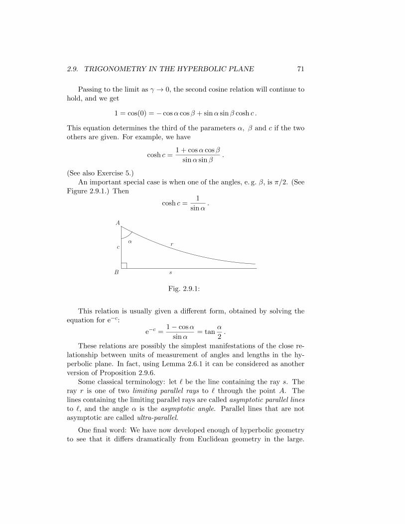
2.9. TRIGONOMETRY IN THE HYPERBOLIC PLANE 71
Passing to the limit as γ → 0, the second cosine relation will continue tohold, and we get
1 = cos(0) = − cosα cosβ + sinα sinβ cosh c .
This equation determines the third of the parameters α, β and c if the twoothers are given. For example, we have
cosh c =1 + cosα cosβ
sinα sinβ.
(See also Exercise 5.)An important special case is when one of the angles, e. g. β, is π/2. (See
Figure 2.9.1.) Then
cosh c =1
sinα.
αc
A
B s
r
Fig. 2.9.1:
This relation is usually given a different form, obtained by solving theequation for e−c:
e−c =1− cosα
sinα= tan
α
2.
These relations are possibly the simplest manifestations of the close re-lationship between units of measurement of angles and lengths in the hy-perbolic plane. In fact, using Lemma 2.6.1 it can be considered as anotherversion of Proposition 2.9.6.
Some classical terminology: let ` be the line containing the ray s. Theray r is one of two limiting parallel rays to ` through the point A. Thelines containing the limiting parallel rays are called asymptotic parallel linesto `, and the angle α is the asymptotic angle. Parallel lines that are notasymptotic are called ultra-parallel.
One final word: We have now developed enough of hyperbolic geometryto see that it differs dramatically from Euclidean geometry in the large.

72 CHAPTER 2. HYPERBOLIC GEOMETRY
However, several results show that in the small, i. e. locally around a point,the geometries become approximations of each other. Examples are thecalculations of area and circumference of a circle, and the remarks on thetrigonometric formulas above. This is analogous to the fact that althoughthe Earth is a sphere, locally it looks flat, and the errors we make by usingEuclidean geometry on small regions are usually very small.
In chapter 5 we shall see that these differences are consequences of thesigns of the curvatures defined by the different metrics.
Exercises for 2.9
1 . In a triangle two of the angles are α and β, and the length of theside opposite to the vertex with angle β is b. Explain how to find theremaining angles and sides.
Why does this establish the congruence criterion SAA?
2. Show that two of the angles of a finite triangle are equal if and only ifthe two sides opposite to these angles have the same length.
3. Use the hyperbolic sine relation to prove that in a hyperbolic trianglethe greatest angle has the longest opposite side.
4. Show that the sides of a triangle all have the same length if and onlyif the three angles also are equal.
If the sides have length a and the angles are α, prove the formulae
cosα =cosh a
1 + cosha
cosh a =cosα
1− cosα
2 cosh(a/2) sin(α/2) = 1. (Hint: cut the triangle into two pieces.)
5. Show that if a simply asymptotic triangle has finite angles α and βand finite side c, then β is determined by α and c.
6. Suppose given a quadrilateral with one ideal vertex and three rightangles. Then two of the sides have finite lengths a and b. Show that
1
cosh2 a+
1
cosh2 b= 1 .

2.9. TRIGONOMETRY IN THE HYPERBOLIC PLANE 73
7. Show that in a triangle with γ = π/2 the following formulas hold:
sinα =sinh a
sinh c
cosα =tanh b
tanh c
8. Formulate and prove a ’converse’ of Proposition 2.9.6.
9. Prove that a map H→ H is a Mobius transformation if and only if itis distance preserving.
Appendix. Remarks on the Beltrami–Klein model
Since the Beltrami–Klein model played such an important part at the begin-ning of these notes, we should not end the discussion of hyperbolic geometrywithout some remarks on the missing bits of its geometry.
When we left it, we had all ingredients except congruence. Now we candefine congruence as equivalence under transformations of the form H−1gH,where H is our identification K ≈ D and g ∈Mob(D) . This can be writtenout explicitly, but the formulas are ugly and not very enlightening. How-ever, by Proposition 2.9.6 we now also know that congruence is completelydetermined by the distance measure, so we might instead ask what the dis-tance formula looks like when transported back to K. It turns out that thisquestion does indeed have a nice and interesting answer.
Recall that the set of points of K is the interior of the unit disk in R2,and the ’lines’ of the geometry are the chords in this disk.
Let Z1, Z2 be two points of K. They span a unique chord which hasendpoints P and Q on the boundary circle of K in R2. Let us denote thedistance function on K by dK.
Proposition A.1. dK(Z1, Z2) =1
2| ln |[Z1, Z2, P,Q]||.
Proof. The identification H : K ≈ D is the composition of the verticalprojection from K to the upper hemisphere B with equator disk K andstereographic projection from B to D. Note that K and D coincide as sets.

74 CHAPTER 2. HYPERBOLIC GEOMETRY
Let W1 = H(Z1) and W2 = H(Z2). The endpoints P and Q are leftfixed, so we have by definition
dK(Z1, Z2) = dD(W1,W2) = | ln |[W1.W2, P,Q]|.
Hence the result follows from
Claim 1 : [W1.W2, P,Q]2 = [Z1, Z2, P,Q].
Now we simplify notation and denote by AB both the Euclidean segmentfrom A to B and its Euclidean length |A−B|. Then the equation in Claim1 reads (
W1P
W1Q
W2Q
W2P
)2
=Z1P
Z1Q
Z2Q
Z2P.
Hence Claim 1 is a consequence of
Claim 2 : Let Z be a point on the chord with endpoints P and Q, and let
W = H(Z). Then
(WP
WQ
)2
=ZP
ZQ.
We will prove this by a geometric argument entirely within Euclideangeometry, referring to Figure 2.9.2. Here O is the center of the unit disk,and we have drawn both the K–line and the D–line with endpoints P andQ. Note that the D–line has the radii OP and OQ as tangents. By thedefinition of π and Φ the point W lies on the line between Z and O, so Wmust be the point of intersection between the D–line and Euclidean segmentOZ.
P
QO
Z
Wh
Fig. 2.9.2:

2.9. TRIGONOMETRY IN THE HYPERBOLIC PLANE 75
Consider now the triangles ZPO and ZQO. With ZP and ZQ as basesegments the two triangles have the same heights, and we have
ZP
ZQ=A(ZPO)
A(ZQO),
where the right hand side is the ratio between the areas of the triangles.
Likewise, the triangles ZPW and ZQW have the same heights, so wededuce
ZP
ZQ=A(ZPW )
A(ZQW )=A(ZPO)−A(ZPW )
A(ZQO)−A(ZQW )=A(PWO)
A(QWO).
But the areas in the last fraction can also be calculated with the tworadii OP and OQ as bases, yielding
ZP
ZQ=
12OP · PW sin(∠WPO)12OQ ·QW sin(∠WQO)
=PW sin(∠WPO)
QW sin(∠WQO).
The D–line through P,W,Q is part of a Euclidean circle, hence we canuse the theorem of peripheral angles to obtain
∠WPO = ∠WQZ and ∠WQO = ∠WPZ.
But from the figure we see that
PW sin(∠WPZ) = h = QW sin(∠WQZ).
Combining these observations, we get
PW
QW=
sin(∠WQZ)
sin(∠WPZ)=
sin(∠WPO)
sin(∠WQO).
Substituting this in the expression forZP
ZQabove proves Claim 2.
Remark. Comparing the formula in Proposition A.1 with the formula for dDin (2.7.4), it might look as if dK is just a rescaling of dD. However, this isnot the case. The reason is that the points P,Q (p, q) are not the same inthe two formulas — in Proposition A.1 they are the endpoints of the chordthrough Z1, Z2, but in (2.7.4) they are endpoints of the D–line through thesame points. The only case where they coincide is when Z1 and Z2 lie on acommon diameter. Then we have dK(Z1, Z2) = 1
2dD(Z1, Z2).

76 CHAPTER 2. HYPERBOLIC GEOMETRY
We can also derive a formula analogous to (2.7.6). First we observethat if we identify the underlying sets of K and D with the unit disk in thecomplex plane, the homeomorphism H : K→ D is given by
H(z) =z
1 +√
1− |z|2
(Exercise 5.) Using this we shall show that
Proposition A.2. cosh(dK(z1, z2) =1− 〈z1, z2〉√
1− |z1|2√
1− |z2|2,
where 〈z1, z2〉 is the Euclidean inner product of z1 and z2.
Proof. Write wi = H(zi), i=1,2. A straightforward calculation starting with(2.7.6) for w1, w2 gives
cosh(dD(w1,w2))
=1− |w1|2 − |w2|2 + |w1|2|w2|2
(1− |w1|2)(1− |w2|2)+
2(|w1|2 + |w2|2 − 2〈w1, w2〉)(1− |w1|2)(1− |w2|2)
=(1 + |w1|2)(1 + |w2|2)
(1− |w1|2)(1− |w2|2)− 4〈w1, w2〉
(1− |w1|2)(1− |w2|2)(2.9.2)
Now write w = H(z) =z
y, where y = 1 +
√1− |z|2. Easy calculations
then give y2 + |z|2 = 2y and y2 − |z|2 = 2y(y − 1); hence
1 + |w|2 = 2/y and 1− |w|2 = 2(y − 1)/y.
Clearly we also have 〈w1, w2〉 = 〈z1, z2〉/y1y2. Substituting this in for-mula (2.9.2) proves the proposition.
An application of this result to yet another model for the hyperbolicplane, the hyperboloid model, is given in exercise 6.
The Beltrami–Klein model is not conformal, and angle measure is muchmore complicated. However, one fact is worth noting: it is easy to draw allK–lines which are orthogonal to a given line! We distinguish between twocases:
(1) If the given line is a diameter, the K–lines orthogonal to it are thechords that are orthogonal to it in the Euclidean sense.
(2) Assume the K–line ` is not a diameter, and let its endpoints be Pand Q. The tangents to the circle at ∞ at P and Q intersect in a point W

2.9. TRIGONOMETRY IN THE HYPERBOLIC PLANE 77
`
λ
W
B
P W
Q
K
(b)(a)
Fig. 2.9.3:
outside the unit disk. The K lines orthogonal to ` are the chords containedin Euclidean lines through W . (See Figure 2.9.3a.)
Note that case (1) follows from case (2) by a limiting procedure. There-fore it suffices to consider (2). We will prove this by a geometric argumentusing the hemisphere model B and a little three–dimensional geometry. Cf.Figure 2.9.3b. In this picture we think of K as lying in a standard R2 ⊂ R3,and B ⊂ S2 is the upper hemisphere.
Via vertical projection the K–lines correspond to B–lines, which are cir-cular arcs (semi–circles) which lie in vertical planes and meet the equatorcircle at right (Euclidean) angles. In particular, ` correspond to one suchsemi–circle, which we call λ.
The reason why we pass to B is that the hemisphere model is conformal,since it is related to D by stereographic projection. Therefore we now onlyneed to determine all B–lines which meet λ orthogonally in the Euclideansense.
A B–line γ meets λ orthogonally if and only if its tangent line at theintersection point does. But the union of all the lines meeting the circlecontaining λ orthogonally is easily seen to be a circular cone, and all thelines meet at its vertex. Since the tangents at P and Q in Figure 2.9.3a aretwo such lines, we see that the cone vertex is precisely the vertex W .
It now only remains to observe that since γ lies in a vertical plane, itstangents also lie in this plane. Hence the plane contains W , and its projec-tion to R2 will be a line also containing W . But the K–line correspondingto γ is contained in this line.

78 CHAPTER 2. HYPERBOLIC GEOMETRY
Exercises for Appendix
1. Which kind of curves are ’horocircles’ in K?
2. Verify that inversion in a diameter in K is ordinary reflection in thatdiameter.
3. Show that two hyperbolic lines have a common perpendicular if andonly they are ultra-parallel (end of section 2.9), and show how it canbe constructed in the Beltrami–Klein model.
4. Show that we can parametrize K by (r, θ) 7→ (tanh r cos θ, tanh r sin θ),where r is the hyperbolic distance from the origin. (’Geodesic polarcoordinates’.)
5. Show that if we identify the underlying sets of K and D with the unitdisk in the complex plane, the homeomorphism H : K → D and itsinverse are given by
H(z) =z
1 +√
1− |z|2and H−1(w) =
2w
1 + |w|2.
6. The hyperboloid model of the hyperbolic plane. The hyperboloid in R3
with equation z2− x2− y2 = 1 has two sheets; let L be the one wherez > 0. (Both sheets would work in the following discussion). IdentifyK with the disk where x2 + y2 < 1 in the plane z = 1. Then it iseasy to see that every line through a point in L and the origin in R3
intersects K in exactly one point; in fact, this defines a homeomorphismΨ : L→ K. (In coordinates: Ψ(x, y, z) = (x/z, y/z).) Hence we get amodel for that hyperbolic plane by mapping the geometry of K to Lby Ψ−1.
Show that the metric in L is given by
cosh(dL((x1, y1, z1), (x2, y2, z2))) = z1z2 − x1x2 − y1y2.
Remark. The expression
(x1, y1, z1), (x2, y2, z2)= z1z2 − x1x2 − y1y2
defines a Minkowski inner product on R3. It is not positive definite, butsatisfies the other axioms for a non–degenerate inner product. Observe

2.9. TRIGONOMETRY IN THE HYPERBOLIC PLANE 79
that L is defined as the set of “unit vectors” for this inner product,and the metric dL can now be expressed by
cosh(dL(A1, A2)) = A1, A2 .
Note the similarity with the distance formula on the unit sphere S2 inEuclidean geometry:
cos(dS2(A1, A2)) = 〈A1, A2〉.
The model L is also called the Minkowski model or the Lorentz modelof the hyperbolic plane. It generalizes easily to higher dimensions andleads to the identification of the group of hyperbolic isometries withthe Lorentz group of linear transformations preserving the Minkowskiinner product.

80 CHAPTER 2. HYPERBOLIC GEOMETRY

Chapter 3
Topological Classification ofcompact, closed surfaces
We now move on to study more general two–dimensional objects and theirpossible geometries. Note that our models for Euclidean or hyperbolic ge-ometry are all homeomorphic to ordinary R2, and the geometries consistof some extra structure. Now we will consider objects (topological spaces)which are only locally homeomorphic to R2. Then the extra geometric struc-ture can also be defined locally, and our goal is to study to which extentthese local structures can be pieced together to give a structure on the wholespace. These spaces are the objects we call “surfaces”, and in this chapter weshall concentrate on the topology of such surfaces. The main result is a com-plete classification of those that are connected and compact as topologicalspaces.
To be more precise: A “surface” is here defined as a two–dimensionaltopological manifold, i. e. a Hausdorff topological space such that every pointhas a neighborhood which is homeomorphic to R2. (This is usually expressedby saying that it is locally homeomorphic to R2.)
Here are some examples (we shall see many more later):
(1) R2, S2, T 2 = S1 × S1,
(2) Open subsets of other surfaces, e. g. the models H and D of the hyper-bolic plane,
(3) (x, y, z) ∈ R3 |F (x, y, z) = 0, ∇F (x, y, z) 6= 0, where F is a contin-uously differentiable function on an open subset of R3. Examples of
81

82 CHAPTER 3. CLASSIFICATION OF SURFACES
this type include graphs of functions of two variables.
(4) Analogous to (3) we can also consider the zero set of a complex ana-lytic function f(z, w) of two variables where at least one of the partialderivatives is different from 0. These are complex curves, but fromour real point of view they have dimension 2 and will be considered assurfaces.
A surface is a disjoint union of its connected components, so it sufficesto classify connected surfaces. Therefore, from now on we assume that allour surfaces are connected. (The word “closed” in the title means that wedo not here consider surfaces with boundary.)
An important operation on surfaces (and manifolds in general) is con-nected sum: Given two surfaces M1 and M2, we can get another by removingan open disk from each of them and gluing the rest along their boundarycircles. More precisely: Let D2 be the closed 2–disk with boundary S1, andlet hi : D2 → Mi, i = 1, 2 be two embeddings, — i. e. maps which arehomeomorphism onto their images. Then the connected sum of M1 and M2,denoted M1 #M2, is defined to be the surface
M1 #M2 = (M1 − h1(intD2)) ∪f (M2 − h2(intD2)) ,
where f : h1(S1)→ h2(S1) is the homeomorphism h2h−11 .
Clearly, M1#M2 ≈ M2#M1. (The symbol ≈ means ”is homeomorphicto”.)
Remark 3.1.7. This construction makes sense also in higher dimensions, butthe result may depend on our choice of h1, h2. However, for surfaces allchoices turn out to give homeomorphic results. This will be clear after wehave proved the classification theorem.
In the following we will use the notation M ≈ N for “M is homeomorphicto N”. Note, in particular, that M#S2 ≈ M for any surface M . It is alsoclear that we can iterate this operation and form the connected sum ofseveral surfaces. The classifications theorem in dimension 2 states that acompact, connected surface is either homeomorphic to a sphere S2, or it canbe written as a connected sum of finitely many copies of only two distinctirreducible surfaces — i. e. surfaces which can not be decomposed further.These two surfaces are the torus T 2 and the projective plane P 2. We willuse the following models for T 2 and P 2:
T 2 is defined as S1×S1, but since S1 is homeomorphic to a closed interval(e. g. [0, 1]) where we have identified the endpoints, we can also think of T 2

83
1M − h (int D) 1 n f
M − h (int D) n
2 2
Fig. 3.1.1: Connected sum
as [0, 1]× [0, 1] where we identify opposite sides pairwise, as indicated on fig.3.1.2.
−1
−1
b
aa
b
Fig. 3.1.2: Torus
The projective plane is obtained from the 2–sphere S2 by identifyingantipodal points. Then we identify every point in the upper hemispherewith a point in the lower hemisphere, hence we only need one of them torepresent all of P 2. Since both hemispheres are homeomorphic to the diskD2, we get P 2 by identifying antipodal points on the boundary circle S1.This identification can be realized by cutting the boundary circle into twointervals and identifying as in fig. 3.1.3.
Note that we have described both the torus and the projective plane asidentification spaces where we start with a 2n-gon (n = 2 and 1 in theseexamples) and identify the sides pairwise according to some definite pattern.

84 CHAPTER 3. CLASSIFICATION OF SURFACES
aa
Fig. 3.1.3: P 2
The labels a, a−1 etc. on the boundary indicate that we identify the twosides in a way that preserves (. . . a . . . a . . . ) or reverses (. . . a . . . a−1 . . . ) thedirection around the 2n-gon. Thus, T 2 is represented by the string aba−1b−1
and P 2 by aa. Another example is the Klein bottle K2, represented byabab−1. This surface is not homeomorphic to a subset of R3, but fig. 3.1.4 isa picture with one circle of self–intersections. Using just the two surfaces T 2
b
aa
b−1
Fig. 3.1.4: Klein bottle
and P 2 and connected sum, we will see that we obtain all other surfaces upto homeomorphism. T 2#T 2, for example, is a surfaces with “two holes”, asin fig. 3.1.5. In the same way, the connected sum of n copies of T 2 becomesa surface with “n holes”.
Fig. 3.1.5: T 2#T 2

85
How can we show that T 2 and P 2 are not homeomorphic? The simplestis probably to observe that T 2 is orientable and P 2 is not. An intuitiveway of thinking about orientability of surfaces is as follows: Consider anembedded curve ω : [a, b] → M . Locally at any point we can distinguishbetween the two sides of the curve and e. g. name them “right” and “left”.Moving along the curve, we can extend this and define the right and left handside of the whole curve. However, if the curve is closed, i. e. ω(b) = ω(a),the notions of right and left obtained when we come back to the startingpoint may not coincide with those we had at the beginning. An example ofthis is the Mobius band, shown in fig. 3.1.6. The arrows indicate a choiceof side locally, but we see that no continuous choice is valid for the wholecurve. We say that the curve is one–sided.
Fig. 3.1.6: Mobius band
If a surface has a one–sided curve, it is called non–orientable, and if allclosed curves are two–sided, it is orientable. It is clear that homeomorphicsurfaces are either both orientable or both non–orientable.
In fact, if M has a one–sided embedded, closed curve, a neighborhoodof this curve looks like a Mobius band. Hence we have
Lemma 3.1.8. A surface is non–orientable if and only if it contains aMobius band.
P 2 is non–orientable, since it contains a Mobius band. This can be seenby doing the identification in fig. 3.1.3 on a band going across the disk fromthe upper to the lower half–circle. To prove that T 2 or any other surface isorientable is harder, since we have to check a certain property for all closedcurves. But here is at least a heuristic argument:
T 2 has a representation in R3 which is two–sided in the sense that itseparates R3 into two components. A choice of one of these makes it possible

86 CHAPTER 3. CLASSIFICATION OF SURFACES
to define right and left hand sides of an embedded curve, “as seen from”the chosen component. One way to do this is to let the ordered triple ofdirections (“right, forward (moving along the curve) and up”) be chosenaccording to the right hand rule in R3. But this choice will not change whenwe move around the curve, so the curve is also two–sided on the surface.Hence T 2 is orientable.
Remark 3.1.9. This also proves that P 2 does not have a two–sided repre-sentation in R3. In fact, one can show that it has no embedding in R3
whatsoever.
We can now state the existence part of our classification theorem:
Theorem 3.1.10. Any compact, connected surface is homeomorphic to afinite connected sum of tori and projective planes.
Proof. To prove this we need a result by Rado from 1925, saying that everysurface can be triangulated. This means that it is homeomorphic to a unionof triangles, where every edge of every triangle is linearly identified withexactly one edge of another triangle. This is a deep result, but not verysurprising. (However, the analogous statement in higher dimensions is falsefrom dimension 4 on!)
Let ∆1, . . . ,∆n be the triangles in a triangulation of a compact surfacesM . We may choose the ordering such that ∪j<i∆j and ∆i have at least oneedge in common, and we choose such an edge Ei for every i. Let
Fk = ∆1 ∪E1 ∆2 ∪ · · · ∪Ek−1∆k,
for k = 1, 2, . . . , n. Then Fk = Fk−1∪Ek∆k, and an easy induction argumentshows that each Fk is homeomorphic to a 2-disk D2, which we may thinkof as a (k + 2)–gon. In particular, Fn will be an (n + 2)–gon, and M isobtained by identifying its edges pairwise. (It follows that n+ 2, hence alson, is even!)
We now give the edges names a, b, . . . , such that the edges which areidentified get either the same (. . . a . . . a . . . ) or “inverse” (. . . a . . . a−1 . . . )names, depending on whether they are identified in a way that preserves orreverses direction around the (n + 2)-gon. (Cf. the descriptions of T 2, K2
and P 2 above.)
If the word W = a . . . a±1 . . . lists the edges counterclockwise, we willwrite D2/W for the result of the identifications. Thus the torus abovecan be written D2/aba−1b−1 and P 2 as D2/aa, whereas S2 is homeomor-phic to D2/aa−1. We let W−1 denote the same word read clockwise, e. g.(abc−1)−1 = cb−1a−1.

87
Let us call a word W defining a surface as above admissible. It is conve-nient to allow the empty word and define D/ = S2. The proof of thetheorem is based on the following lemma:
Lemma 3.1.11. (i) If W = W1W2, then D2/W1W2 = D2/W2W1.
(ii) If W1 and W2 are admissible, then W1W2 is also admissible, and
D2/W1W2 ≈ D2/W1 #D2/W2
Proof. (i) is only the observation that when we go around the disk, it doesnot matter where we start reading the word.
(ii) We cut D2 along a line c connecting the two endpoints on the bound-ary where W1 and W2 meet. (See fig. 3.1.7.) Since W1 and W2 are admis-sible, these two endpoints are identified, and c represents a closed curve inD2/W1W2.
D − disk2
1/W D2
1/W W 2D − disk2
2/W
1W
2W 2W
1W
c c c
Fig. 3.1.7:
Thus we get two new disks where the edges are given by W1 and W2,respectively, plus an extra edge c in both. It is then easy to see that if weperform the identifications encoded by W1 and W2 in these two disks butdo not identify the c’s, we get spaces homeomorphic to (D2/W1 − disk) and(D2/W2 − disk).
We may construct D2/W1W2 by first performing all the identificationsin the two parts and then gluing along the dashed curves (which now havebecome circles). But this is clearly D2/W1 #D2/W2.
In particular, we have

88 CHAPTER 3. CLASSIFICATION OF SURFACES
(1) D2/Waa−1 ≈ D2/W #S2 ≈ D2/W
(2) D2/Waa ≈ D2/W #P 2
(3) D2/Waba−1b−1 ≈ D2/W #T 2
Therefore we can eliminate all sequences having the form aa−1, aa andaba−1b−1, in the sense that we can write D2/W ≈ D2/W ′#M ′, where M ′
is a connected sum of tori and projective planes, and W ′ is a word which isat most as long as W and which does not contain any such strings.
Suppose now that W = W1aW2a. Then we may, as in the proof of thelemma above, cut D2 into two disks separating the words W1a and W2a.But this time we construct the surface by first gluing back along the edgeslabeled a. The result is a new disk with edge–identification given by theword W1W
−12 cc.
1W2W1W
2W
a
a
c−1
a
c
c
Fig. 3.1.8:
Hence we also have
(4) D2/W1aW2a ≈ D2/W1W−12 cc ≈ D2/W1W
−12 #P 2
Example 3.1.12. The Klein bottle can be represented as D2/bab−1a, whichby (4) is homeomorphic to D2/bb#P 2 ≈ P 2#P 2.
By repeated use of (2) and (4) we now reduce to the case where all theedges occur in pairs (c, c−1) etc., and by (1) we may eliminate all strings oftype cc−1 (and c−1c). Then we must either have M ≈ S2, or we can find(possibly after switching the labels c and c−1 and/or d and d−1) edges c andd occurring in the order c . . . d . . . c−1 . . . d−1 . . . in the word W . (Choosefirst a pair with minimal distance between them.)
We now cut and paste as in fig. 3.1.9.
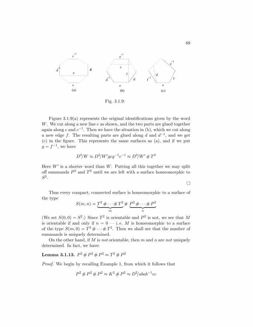
89
−1d
−1c
−1d
−1e
−1f
−1e
d
c
e
e
d
(a) (b)
df
c
df
e
(c)
Fig. 3.1.9:
Figure 3.1.9(a) represents the original identifications given by the wordW . We cut along a new line e as shown, and the two parts are glued togetheragain along c and c−1. Then we have the situation in (b), which we cut alonga new edge f . The resulting parts are glued along d and d−1, and we get(c) in the figure. This represents the same surfaces as (a), and if we putg = f−1, we have
D2/W ≈ D2/W ′geg−1e−1 ≈ D2/W ′#T 2
Here W ′ is a shorter word than W . Putting all this together we may splitoff summands P 2 and T 2 until we are left with a surface homeomorphic toS2.
Thus every compact, connected surface is homeomorphic to a surface ofthe type
S(m,n) = T 2 # · · ·#T 2︸ ︷︷ ︸m
# P 2 # · · ·#P 2︸ ︷︷ ︸n
(We set S(0, 0) = S2.) Since T 2 is orientable and P 2 is not, we see that Mis orientable if and only if n = 0 — i. e. M is homeomorphic to a surfaceof the type S(m, 0) = T 2 # · · ·#T 2. Then we shall see that the number ofsummands is uniquely determined.
On the other hand, if M is not orientable, then m and n are not uniquelydetermined. In fact, we have:
Lemma 3.1.13. P 2 #P 2 #P 2 ≈ T 2 #P 2
Proof. We begin by recalling Example 1, from which it follows that
P 2 #P 2 #P 2 ≈ K2 #P 2 ≈ D2/abab−1cc

90 CHAPTER 3. CLASSIFICATION OF SURFACES
Successive applications of Lemma 3.1.11 and the homeomorphism (4)give
D2/abab−1cc ≈ D2/abacbc ≈ D2/acbcab ≈ D2/aca−1c−1bb ≈ T 2 #P 2
Now we are ready to complete the classification theorem:
Theorem 3.1.14. Any compact, connected surface M is homeomorphic toa surfaces of the type S(m,n), where n = 0, 1 or 2. m and n are thenuniquely determined by M .
Proof. The existence follows from Theorem 3.1.10 and Lemma 3.1.13, so itonly remains to establish the uniqueness of n and m. We can not give allthe details here, but at least we can explain the invariants we use and theingredients of the proof.
The invariants are orientability and the so–called Euler characteristic.We have already introduced orientability, and it is obvious that homeo-
morphic surfaces are either both orientable or both no–orientable.The Euler characteristic is an integral invariant which can be associated
to any triangulated surface M . If the triangulation has s triangles, e edgesand v vertices, then the Euler characteristic is defined by
χ(M) = v − e+ s .
The fundamental fact is that this number is independent of which triangu-lation we use, such that if M and N are homeomorphic, then χ(M) = χ(N).This is the only fact we cannot prove here, in full generality, but it is a niceexercise to show that the Euler characteristic does not change if we subdi-vide the triangles in a given triangulation by introducing new vertices andedges. (Exercise 9. The missing step to the general result is then to showthat we can go from one triangulation to any other by a finite number ofsuch operations or their inverses.)
Using suitable triangulations of the identification models D2/W it is notdifficult to verify that
χ(S(m,n)) = 2− 2m− n
This means that if M is orientable, then χ(M) = 2− 2m. Hence m, andtherefore also M , is determined by χ(M).
If M is non–orientable, then n = 1 or 2, and χ(M) = 1−2m or −2m. Inthe first case χ(M) is odd (n = 1), and in the second case it is even (n = 2).In both cases χ(M) determines both m and n.

91
Remark 3.1.15. Note that we also have proved that M is completely deter-mined by χ(M) and whether M is orientable or not.
In the orientable case the number m is called the genus of the surface.It also follows that the genus determines an orientable surface up to home-omorphism.
Exercises for 3.1
1. Show that if B is a Mobius band with boundary circle S, then
P 2 ≈ B ∪S≈S1 D2
K2 ≈ B ∪S B
2. Show that S(m,n) can be represented asD2/[a1, b1] · · · [am, bm]c21 · · · c2
n,where [a, b] = aba−1b−1 and c2 = cc.
3. In the identification space D2/W the edges of D are identified pairwisewith each other to curves on the surface. Draw these curves on S(2, 0)in fig. 3.1.5 if we use the identifications in exercise 2.
4. Verify the formula χ(S(m,n)) = 2− 2m− n.
Determine the Euler characteristics of S2, T 2, P 2 and K2.
Show that these are the only compact, connected surfaces having Eulercharacteristic ≥ 0.
5. Determine which compact surface can be represented asD2/abc−1bdacd−1.What is its Euler characteristic? Is it orientable?
6. Show that if M1 and M2 are compact surfaces such that M1#M2 ishomeomorphic to M1, then M2 must be homeomorphic to S2.
7. Show that χ(M#N) = χ(M) + χ(N)− 2 for all compact surfaces Mand N .
A surface is called irreducible if the only way it can be written asa connected sum is if one of the summands is S2. Prove that M isirreducible if and only if M is homeomorphic to T 2, P 2 or S2
8. Generalize the notion of triangulation to allow the two–dimensionalpieces to be arbitrary n–gons for all n. Show that the formula
χ(M) = v − e+ s

92 CHAPTER 3. CLASSIFICATION OF SURFACES
still holds, where now s is the number of polygons.
9. Show that χ(M) does not change under subdivision of the triangula-tion. (A triangulation τ2 is a subdivision of a triangulation τ1 if everysimplex of τ2 is contained in a simplex of τ1.)

Chapter 4
Geometry on surfaces —basic concepts
4.1 Introduction, local structure
Our goal is to generalize our geometrical studies from plane geometries togeometries on surfaces. As we already have pointed out, this requires morestructure, so we begin by discussing what it means to put structure ona surface. The word “structure” is here used somewhat loosely, but theexamples below will, hopefully, make it clearer what we mean.
Recall that a surface M is locally homeomorphic to R2. This meansthat M has an open covering Ujj∈J such that there are homeomorphismsxj : Uj ≈ xj(Uj) ⊂ R2, where xj(Uj) is open in R2. Such a pair (Uj , xj) iscalled a (local) chart on M and (Uj , xj)j∈J is called an atlas.
If we have some kind of structure on (subspaces of) R2 (e. g. complex,Euclidean, hyperbolic, . . . ), a natural thing to try is to transfer this structureto M via the local charts. Of course, this ought to be independent of whichchart we choose, so the problem, in general, will be compatibility in theoverlaps between two or more charts.
Example. The fundamental example, and also the model for any furtherdiscussion, is that of a differentiable structure. It is clearly of great interest toextend the concept of derivatives and differentiable functions to surfaces (ormore general manifolds). Using the philosophy above, a function f : M → Rshould be differentiable at a point p ∈ M if fx−1
j is differentiable at xj(p),where (Uj , xj) is a chart with p ∈ Uj . But if (Ui, xi) is another chart withp ∈ Ui, this should be the same as requiring that fx−1
i is differentiable at
93

94 CHAPTER 4. GEOMETRY ON SURFACES
xi(p). These two conditions are equivalent for every function f if and onlyif xix
−1j and xjx
−1i are differentiable at xj(p) and xi(p), respectively. Hence
we have a well defined concept of “differentiable function on M” if and onlyif M has an atlas (Uj , xj)j∈J such that the coordinate transformationsxjx−1i are differentiable wherever they are defined (i. e. in xi(Ui ∩ Uj)) for
all i and j. Such an atlas is called a differentiable atlas, and it defines adifferentiable structure on M .
However, if studying differentiable functions is the motivation for in-troducing this structure, we should identify structures coming from atlasesdefining the same set of such functions. We call two atlases equivalent if theydo, and define a differentiable structure to be an equivalence class of differ-entiable atlases. It is easy to see that two atlases (Ui, xi) and (Vj , yj)are equivalent if and only if
• all compositions yjx−1i and xiy
−1j are differentiable.
But this condition is clearly equivalent to
• (Ui, xi) ∪ (Vj , yj) is also a differentiable atlas.
The set of all differentiable atlases (as sets of charts) is partially orderedby inclusions, and it follows that the union of all atlases in an equivalenceclass is the unique maximal element in that class. Therefore we can alsoidentify a differentiable structure with a maximal differentiable atlas.
A surface M with a choice of such structure is called a differentiablesurface.
Remark. There is nothing in this discussion that confines it to dimensiontwo. It applies to manifolds of arbitrary dimensions — just replace ‘R2’ by‘Rn’ everywhere — and defines a differentiable manifold.
We may also require more: if, e. g. , all the coordinate transformationsare r times continuously differentiable, we have a Cr–structure. Here r mayeven be ∞, and a surface (manifold) with a C∞–structure is called smooth.
Thus, if M has a differentiable structure, we can talk about differentiablefunctions on M . But we can also define differentiable mappings between suchmanifolds. If M and N are two manifolds with Cr-structures (Ui, xi) and(Vj , yj) and f : M → N is a mapping, we say that f also is Cr if all themappings yjfx
−1i are r times continuously differentiable wherever they are
defined.
This way we can transfer concepts and results having to do with dif-ferentiation to manifolds, provided they are equipped with differentiablestructures. We can also define real analytic manifolds and maps, and re-placing Rn with Cn in the definitions, we arrive at the concept of complex

4.2. GEOMETRIC STRUCTURE ON SURFACES 95
analytic structures.
If f : M → N is differentiable and also has a differentiable inverse, wesay that f is a diffeomorphism and that M and N are diffeomorphic. Thenthey are, of course, also homeomorphic. One can show that all surfaces havesmooth structures that are unique up to diffeomorphism. Hence there is noloss of generality when we from now on tacitly assume that all surfaces aresmooth.
4.2 Geometric structure on surfaces
Using these ideas we will now attempt to define a geometric structure ona surface M to be a geometry on (subsets of ) R2 together with a (differ-entiable) atlas on M such that all the coordinate transformations preservethis geometry. This will become more precise as we proceed, but first welook at some examples.
Example 1. If we consider the integers Z as a subgroup of the additivegroup R, we can define the torus T 2 as the quotient group R2/Z2 (with thequotient topology). The easiest way to see this is to observe that underaddition of elements of Z2, every element of R2 can be moved to an elementin [0, 1]× [0, 1], and the only identifications here are of the form (t, 0) ∼ (t, 1)or (0, s) ∼ (1, s). This means that the quotient is the disk D = [0, 1]× [0, 1]with boundary identifications according to the pattern aba−1b−1.
The quotient map p : R2 → T 2 is a local homeomorphism, since
p|(a, b)× (c, d) : (a, b)× (c, d)→ p((a, b)× (c, d))
is a homeomorphism whenever b−a < 1 and d−c < 1. If we use the inversesof these homeomorphisms as charts, the coordinate transformations will looklike (s, t) → (s + m, t + n) for integers m and n. Here (m,n) will dependcontinuously on (s, t), and are therefore locally constant.
These coordinate transformations are restrictions of Euclidean isometries(congruences), and they preserve the Euclidean geometry — i. e. they takelines to lines and preserve lengths and angles. Therefore this atlas defineswhat we may call a Euclidean structure on T 2.
The images of straight lines in R2 define a system of curves on T 2 whichwe again may call “lines” in the Euclidean structure. This set of lines will,however, not satisfy all of Hilbert’s axioms. For example, lines in R2 withrational slope will map to closed curves on T 2 — hence betweenness willhave no meaning — while lines with irrational slope will map injectively to

96 CHAPTER 4. GEOMETRY ON SURFACES
a topologically dense subset of T 2. Two distinct curves may intersect inmore than one point, even infinitely many, and there will be infinitely manysuch curves going through two given points.
This means that segments are not determined by their endpoints, but wehave to also specify the lines containing them. Likewise, triangles are notdetermined by the three vertices only. The best way to define such geometricconcepts is to lift them to R2 and use the geometry there.
Angular measure between two lines, however, will have a unique mean-ing, since we get the same value, independent of which chart we use. We mayalso measure Euclidean distance along lines, but this will only be uniquelydetermined in small neighborhoods, since lines may be closed. But thismakes it possible to compare two arbitrary segments, and we may for in-stance, as in Hilbert’s axiom C1, find a congruent copy of any given segmentstarting in any point and going in any direction.
This last property is closely related to a property called “completeness”,saying that we may prolong any segment as far as we want. For instance,if M is the complement of a point in T 2 (or R2), then M will obviouslyinherit a Euclidean structure in the sense that we can find an atlas whereall the coordinate transformations are restrictions of Euclidean isometries,but this structure will not be complete, since segments on lines puncturedby the missing point can not be prolonged across it. We will essentially onlybe interested in complete structures.
If we replace Z2 by another additive subgroup Λ ⊂ R2 of rank 2, thenR2/Λ will also have a Euclidean structure. R2/Λ will be homeomorphic (evendiffeomorphic) to T 2, but it may not be possible to find a homeomorphismwhich preserves the structure — i. e. the Euclidean structures may not beequivalent for different Λ.
To obtain these structures we have used the additive group structure onR2, but if we look closer, we see that what we really have used is only thatZ2 (or Λ) is a group acting via structure preserving diffeomorphisms of thesurface R2. From this point of view we could replace R2 by any surface Xwith a structure (“geometry”) and Z2 by a group Γ of diffeomorphisms of Xpreserving this structure (“congruences”), provided that the quotient spaceX/Γ is a surface. The next examples are of this type.
Example 2. Again we let X = R2 with Euclidean geometry, but now we letΓ be the group of Euclidean isometries (congruences) generated by γ(s, t) =(s + 1, t) and τ(s, t) = (−s + 1, t + 1). As with the torus, we can showthat the quotient map R2 → R2/Γ is a homeomorphism when restricted toopen rectangles with sides less than 1, and the inverses of these give an atlas

4.2. GEOMETRIC STRUCTURE ON SURFACES 97
which defines a Euclidean structure. To see which surface R2/Γ is, we firstobserve that γ identifies all the vertical bands [n, n + 1)× R via horizontaltranslation. τ identifies all the horizontal bands R× [n, n+ 1), but in a waysuch that every other band is reflected in the line 1/2×R. Hence we alsoobtain R2/Γ from the square [0, 1] × [0, 1], but now we identify the sidesaccording to the pattern ’abab−1’. Thus the quotient is a Klein bottle.
Example 3. In this example, we use a different surface than R2 to modela geometry. We say that a surface has spherical structure if it is locallyhomeomorphic to the sphere S2 in such a way that the coordinate trans-formations are restrictions of spherical congruences, i. e. multiplication bymatrices in the orthogonal group O(3). It turns out that there is only oneexample of such a geometry except S2 itself; namely the projective planeP 2. But P 2 is, in fact, of the type X/Γ. In fact, let X = S2, and letΓ = Z/2 = ±I ⊂ O(3), which acts on S2 via the antipodal map. Thenthe quotient is precisely P 2, and the restrictions of the quotient map to opensubsets contained in hemispheres are homeomorphisms. If we use these todefine an atlas, then the coordinate transformations are either identities orrestrictions of the antipodal map. These are both orthogonal, hence we havedefined a spherical structure.
As remarked when we discussed Hilbert’s axiom system for plane geome-tries, the spherical geometry is also characterized by a system of “lines”,namely the great circles in S2 or the images of those in P 2 (which also be-come circles). This defines an incidence geometry on P 2 where any two lineswill intersect in exactly one point. This geometry is complete.
Two observations before we go on:
(i) In all the examples so far we have described the surfaces by a rep-resentation D2/W of the type we used to classify surfaces. Notice that inthe concrete models used for D2, it appears as a polygon bounded by linesin the relevant geometry, and the identifications given by the word W aregiven by elements in a group Γ.
(ii) The concrete models for D2 are not uniquely determined — noteven up to congruence. (For the torus we could, for example, have useda parallelogram with vertices (0,0), (1,1), (1,2) and (0,1).) But all choiceswill have the same area. Therefore it is meaningful to say that the quotientsurface also has this area.
Example 4. It should now be clear how we should define what it should meanfor a surface M to have a hyperbolic structure. Motivated by the examplesabove, we should look for examples of the form H/Γ or D/Γ, where Γ is a
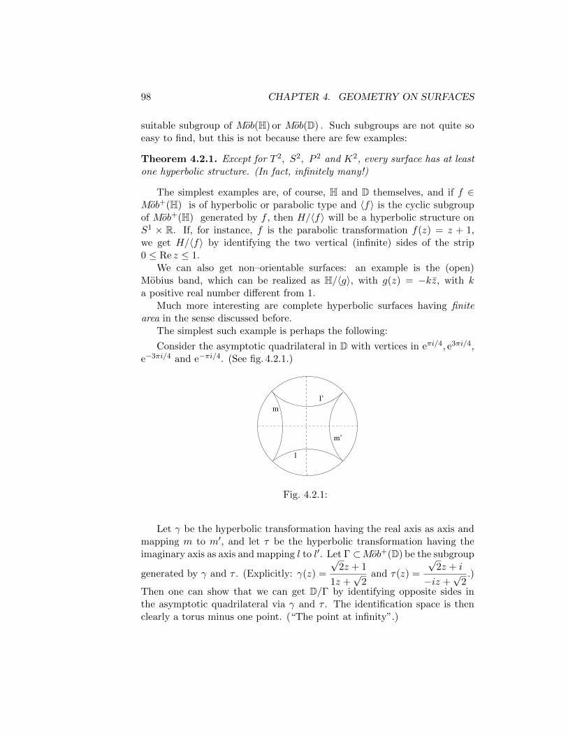
98 CHAPTER 4. GEOMETRY ON SURFACES
suitable subgroup of Mob(H) or Mob(D) . Such subgroups are not quite soeasy to find, but this is not because there are few examples:
Theorem 4.2.1. Except for T 2, S2, P 2 and K2, every surface has at leastone hyperbolic structure. (In fact, infinitely many!)
The simplest examples are, of course, H and D themselves, and if f ∈Mob+(H) is of hyperbolic or parabolic type and 〈f〉 is the cyclic subgroupof Mob+(H) generated by f , then H/〈f〉 will be a hyperbolic structure onS1 × R. If, for instance, f is the parabolic transformation f(z) = z + 1,we get H/〈f〉 by identifying the two vertical (infinite) sides of the strip0 ≤ Re z ≤ 1.
We can also get non–orientable surfaces: an example is the (open)Mobius band, which can be realized as H/〈g〉, with g(z) = −kz, with ka positive real number different from 1.
Much more interesting are complete hyperbolic surfaces having finitearea in the sense discussed before.
The simplest such example is perhaps the following:
Consider the asymptotic quadrilateral in D with vertices in eπi/4, e3πi/4,e−3πi/4 and e−πi/4. (See fig. 4.2.1.)
l
l’
m’
m
Fig. 4.2.1:
Let γ be the hyperbolic transformation having the real axis as axis andmapping m to m′, and let τ be the hyperbolic transformation having theimaginary axis as axis and mapping l to l′. Let Γ ⊂Mob+(D) be the subgroup
generated by γ and τ . (Explicitly: γ(z) =
√2z + 1
1z +√
2and τ(z) =
√2z + i
−iz +√
2.)
Then one can show that we can get D/Γ by identifying opposite sides inthe asymptotic quadrilateral via γ and τ . The identification space is thenclearly a torus minus one point. (“The point at infinity”.)

4.2. GEOMETRIC STRUCTURE ON SURFACES 99
This means that if p is a point on the torus T 2, then T 2 − p has ahyperbolic structure of the form D/Γ, with finite area equal to 2π. (Theasymptotic quadrilateral is the union of two triply asymptotic triangles in-tersecting in one side.)
We can also use fig. 4.2.1 to describe another example: Let γ be aparabolic transformation which identifies l and m and fixes e−3πi/4, andlet τ be a parabolic transformation which identifies l′ and m′ and fixes eπi/4.Then we get D/ < γ, τ > by identifying l with m, and l′ with m′. Thissurface is homeomorphic to a sphere were we have removed three points.(Alternatively R2 minus two points.) Hence this surface also has a hyper-bolic structure of the form D/Γ, with finite area equal to 2π.
Both of these examples are complete. In both examples the group Γis a free group on two generators. (Isomorphic to the so–called fundamen-tal group of the surface). But the surfaces are not homeomorphic, so theabstract group does not determine the surface up to homeomorphism.
The hyperbolic surfaces constructed so far have all been non–compact.The simplest compact surfaces admitting a hyperbolic structure are of genustwo (i. e. they are homeomorphic to T 2#T 2), and we now sketch how onecan construct such examples.
From the proof of the classification theorem, we know that a surface ofgenus two can be obtained from an octagon where the edges are identifiedaccording to the pattern a1b1a
−11 b−1
1 a2b2a−12 b−1
2 . We now need this to be ahyperbolic octagon, where the identifications are made via hyperbolic isome-tries. In particular, we need the edges that are identified (e. g. the edgeslabeled a1 and a−1
1 ) to be segments of the same length. Moreover, all thevertices are identified to one point and all angles are preserved, so the sumof the interior angles at all vertices must be 2π. But in the hyperbolic planewe may achieve this by a regular octagon. In the disk model this can beconstructed as follows: Draw the radii (the rays) from 0 ∈ D to the eightpoints ekπi/4k=0,...,7 in S1. Every circle in D with center at 0 will intersectall these radii, and the eight points of intersection will be the vertices ofa regular, hyperbolic octagon. When the (hyperbolic) radius of the circleincreases from 0 to ∞, the interior angle at the vertices will decrease from3π/4 (as in the Euclidean case) to 0 (with all the vertices at∞). Somewherein between the angle will be π/4, which is what we need. (We can, of course,also use the hyperbolic trigonometric relations to calculate exactly for whichradius this will happen.)
We now use this octagon as our disk D2. Then there are unique elementsγi ∈Mob+(H) mapping ai to a−1
i , i = 1, 2, and τi ∈Mob+(H) mapping bi

100 CHAPTER 4. GEOMETRY ON SURFACES
to b−1i , i = 1, 2, with the right orientations. If we identify the edges of D2
by these congruences, the identification space becomes a surface of genustwo with a hyperbolic structure. This surface also has the form D/Γ, wherenow Γ is generated by the elements γ1, γ2, τ1 and τ2.
The area of this surface is equal to the area of the regular octagon D2,i. e. 4π.
This hyperbolic structure is also complete, and the “lines” are images ofD-lines under the quotient map D→ D/Γ.
Remark 4.2.2. From the formula for the area of hyperbolic triangles it is easyto see that an n–gon with peripheral angle sum 2π has area (n − 4)π. Itfollows that the area of a compact hyperbolic surface of genus g constructedas above from a 4g–gon will have area 4π(g − 1), independent of lengths ofthe sides. This will later be a consequence of a much more general result —the Gauss–Bonnet theorem.
After all these examples, we are now ready for a more formal definition:Let (X,G) be one of the pairs
• (H,Mob(H)) (or (D,Mob(D)),
• (R2, E(2)), where E(2) is the group of Euclidean isometries,
• (S2, O(3)), where O(3) is the group of spherical isometries (orthogonalmatrices).
We say that a surface has a geometric structure modeled on (X,G) (orshorter: a hyperbolic, Euclidean or spherical structure, respectively) if ithas an atlas (Ui, xi : Ui → xi(Ui) ⊂ X)i such that all the coordinatetransformations are restrictions of elements of G.
One can show that a complete, connected surface with such a structuremust have the form X/Γ for some subgroup Γ ⊂ G. The classification ofgeometric structures on surfaces then becomes the classification of subgroupsoccurring this way. The richest and most interesting such theory is in thehyperbolic case, were it leads to the theory of Fuchsian groups.
The idea of characterizing geometries using group actions goes back toFelix Klein and Sophus Lie, and it was presented by Klein in the famousErlangen program in 1872. The groups G are examples of Lie groups. Notethat in all the three cases above G acts transitively on X, i. e. for any twopoints x, y ∈ X we can find a g ∈ G such that y = gx. Moreover, thestabilizer subgroup
Gx = g ∈ G|gx = x

4.2. GEOMETRIC STRUCTURE ON SURFACES 101
is isomorphic to the orthogonal group O(2). Then, for any x ∈ X, the map
g 7→ gx : G→ X
induces a bijection (even a homeomorphism) between X and the left cosetsG/Gx, with G–action corresponding to left multiplication. This way weobtain identifications
R2 ≈ E(2)/O(2),
S2 ≈ O(3)/O(2),
H ≈ SL2(R)/SO(2).

102 CHAPTER 4. GEOMETRY ON SURFACES

Chapter 5
Differential geometry onsurfaces
We are now going to broaden our perspective and generalize dramaticallythe idea of geometric structures on surfaces. Until now we have restrictedourselves to the classical geometries or structures built from them. But thegeometries of most surfaces in space are not of this nature — still they arevery natural objects for geometric studies, and we would like to develop atheory which also includes these. This will require completely new ideas,exploiting methods from calculus and differential equations — whence theterm differential geometry. The structures built from the classical geometriesare very special cases, and one of our main results will be a characterizationof these geometries inside differential geometry.
The geometric structures we defined earlier were homogeneous; they look“the same” at every point in the sense that neighborhoods of any two pointscan be mapped to each other by local congruences, as, for instance, on aperfectly round sphere in space. However, most surfaces are not like this.On a two–dimensional graph a maximum point and a saddle point lookvery different, and whatever we may mean by “geometric structure” shouldcapture this difference.
In this chapter we will introduce a notion of geometric structure which isallowed to vary continuously over the surface. This notion will not be basedon lines and incidence, even locally, but rather on infinitesimal versions ofdistance and angles, encoded in a Riemannian metric. Maps preservingthis metric — local isometries — are then analogues of local congruences inthe classical geometries, but we do not require such maps to exist betweenneighborhoods of arbitrary points.
103

104 CHAPTER 5. DIFFERENTIAL GEOMETRY
Although not part of the initial structure, analogues of “lines” in theclassical geometries will appear eventually, but now they will be constructedas curves satisfying local properties that can be used to characterize lines inthe classical geometries (geodesic curves).
The history of differential geometry on surfaces is long and fascinating.The literature is enormous, and we can only begin to explore it in these notes.It started with studies of special surfaces in Euclidean 3–space and onlygradually developed into a general theory. Central characters in the storywere Euler, Monge and, above all, Gauss. Gauss was the first to introducethe intrinsic point of view, realizing that many aspects of geometry could beunderstood from metric properties of the surfaces itself, without referenceto the surrounding space. This paved the way for Riemann, who generalizedthe theory to abstract manifolds of any dimension. In honour of him theabstract theory is also called Riemannian geometry.
Our treatment will be based on the abstract point of view, but usinggeometry on surfaces in space as motivation. After covering the most fun-damental ideas, we will concentrate on two major results: characterizationof the classical geometries and the Gauss–Bonnet theorem.
But before we can venture into this new terrain, we need some morebackground material on differentiable surfaces and maps. Everything willbe formulated for smooth (i. e. C∞) surfaces. We will need to differentiatefunctions several times, and then it is convenient to agree once and for allthat all surfaces and maps are smooth.1
The fundamentals on tangent planes and derivatives are covered in sec-tion 1, followed by a discussion of orientability in section 2. Then we areready for the definition of the fundamental concepts of Riemannian metricsand local isometries, which are found in sections 3 and 4. Section 5 treatsthe most important tool we have for measuring the variation of a metric overa surface: Gaussian curvature. The promised reappearance of distinguishedlines, geodesics, follows in section 6. They are used to construct particu-larly well behaved local coordinates (section 7), which, in turn, are usedin section 8 to characterize the classical geometries as those with constantcurvature. The last section deals with the famous Gauss–Bonnet theorem,which is a powerful formula bringing together topological information (Eulercharacteristic) and curvature.
A remark on terminology: we have defined differentiable structures andmaps using local charts x : V → R2, where the V’s are open subsets of the
1A careful analysis will reveal that as long as we just study surfaces in R3, C2 will do.The extension to abstract surfaces via Gauss’ Theorema egregium requires C3.

5.1. TANGENT PLANES AND DERIVATIVES OF MAPS 105
surface S. It will here be convenient to replace charts with their inversesx−1 : x(V)→ S, which we will call (local) parametrizations. Thus, a surfacecan also be defined as a space S such that for every p ∈ S there is a mapx : U → S from an open set U ⊂ R2, such that p ∈ x(U) and x : U → x(U) isa homeomorphism. (x,U) is also called a coordinate patch. The coordinatetransformation are now the maps y−1x : U ∩ x−1y(V ) → V ∩ y−1x(U),defined for coordinate patches (x,U) and (y,V).
We will here also use the word atlas for a collection of coordinate patches(xi,Ui) such that ∪iUi = S. A differentiable structure on S is then amaximal atlas such the all coordinate transformations are smooth.
We emphasize that this is only a change of language; one can easily passbetween charts and parametrizations by taking inverses.
5.1 Tangent planes and derivatives of maps
We have already defined what it means for a map between smooth surfacesto be smooth, but we also need to define what we mean by the derivativesof such maps. The idea is that the derivative of a map f should be alinear approximation to f , so we first have to define vector spaces whichapproximate the surface: the tangent planes. This can be done in severaldifferent ways, but here our point of view is that tangent vectors should betangent vectors of curves on the surface. To illustrate the idea, let q be apoint in the plane R2. Every smooth curve through q has a tangent vectorthere, and the set of all possible tangent vectors of curves through q cannaturally be identified with the vector space R2 itself. But each vector canbe realized as the tangent vector of infinitely many curves through q. Hence,if we define an equivalence relation on the set of smooth curves through q bydeclaring two curves to be equivalent if they have the same tangent vectorat this point, we can identify the vector space R2 with the set of equivalenceclasses. This is a formulation that is easy to generalize to an arbitrarysmooth surface.
Let S be a smooth surface, and let p be a point on S. By a curve at p weshall mean a smooth map ω : J → S, where J is an open interval containing0, such that ω(0) = p. Let Ωp = Ωp(S) be the set of all such curves at p.
We now choose a local parametrization x : U → S around p. Then x−1ωis a curve at x−1(p) ∈ R2, and (x−1ω)′(0) is a vector in R2. Define theequivalence relation ∼ on Ωp by
ω ∼ τ ⇐⇒ (x−1 ω)′(0) = (x−1 τ)′(0).

106 CHAPTER 5. DIFFERENTIAL GEOMETRY
(Cf. Fig. 5.1.1. Note that ω and τ need not be defined on the same intervalJ for this to make sense. It is also not necessary that the image of the wholecurve is contained in x(U).
x−1(p)
px
U S
Fig. 5.1.1: Curves with the same tangent.
Lemma 5.1.1. (1) The equivalence relation ∼ does not depend on the choiceof local parametrization x.Define TpS to be the set of equivalence classes.
(2) ω 7→ (x−1ω)′(0) induces a bijection TpS ≈ R2.(3) The bijection in (2) defines a vector space structure on TpS which is
independent of x.
Proof. (1): If y : V → S is another parametrization, then
(y−1ω)′(0) = (y−1xx−1ω)′(0) = J(y−1x)x−1(p)(xω)′(0) ,
where J(y−1x)x−1(p) is the Jacobian matrix of y−1x at the point x−1(p).But J(y−1x)x−1(p) is invertible, since y−1x is a diffeomorphism near x−1(p).
(2) Injectivity follows immediately from the definition of ∼.Surjectivity: If v ∈ R2, let ω(t) = x(x−1(p) + tv). Then ω(t) is defined
for t near 0, and (x−1ω)′(0) = v.
(3): Let αx : TpS → R2 be the bijection in (2), and let αy be theanalogous bijection obtained using the parametrization y. Then
αy α−1x (v) = y−1(x(x−1(p) + tv))′(0) = J(y−1x)x−1(p) v.

5.1. TANGENT PLANES AND DERIVATIVES OF MAPS 107
But multiplication by J(y−1x)x−1(p) is an isomorphism of vector spaces.
Definition 5.1.2. TpS with the vector space structure given by Lemma 5.1.1is called the tangent plane of S at p.
This definition is quite abstract, and valid for an arbitrary surface. How-ever, for surfaces in R3, we can identify TpS with something which is easierto visualize.
Definition 5.1.3. Let S be a subset of R3 which is also a smooth surface,and let ι : S ⊂ R3 be the inclusion map. S is called a regular surface if forevery local parametrization x of S the Jacobian of the composition ι x hasrank 2 at every point.
From now on, when we write S ⊂ R3, we will always assume that S isregular.
One can show that S is regular if and only if it locally (around everypoint) has the form (x, y, z) ∈ R3 : F (x, y, z) = 0 for some smooth functionF with ∇F 6= 0 on S. Spheres are examples of surfaces defined this way.Other important examples include graphs of smooth functions f(u, v) definedon open subsets O ⊂ R2, parametrized by x(u, v) = (u, v, f(u, v)). In fact,we shall see below that locally every regular surface can be identified witha graph, possibly rotated and translated in space.
If S is regular, we can identify TpS with the plane in R3 which containsp and all the tangent lines to curves on S through p. This plane can befurther identified with a linear subspace of R3 via the translation taking pto 0 ∈ R3. Thus we may naturally identify every TpS with such a subspace,and we will always assume that we have done so. The vector space structuregiven by Lemma 5.1.1 makes this identification an isomorphism. Note thatif S is given by an equation F (x, y, z) = 0, the tangent space is determinedby its normal vector ∇F (x, y, z).
Notation. Let ω′(0) denote the equivalence class of ω in TpS. This is thetangent vector of ω in p. More generally, we let ω′(t) denote ω′t(0), whereωt(s) = ω(t+s) (where this is defined). This means that we take the tangentvector of ω in ω(t) instead of ω(0). Note that if S ⊂ R3, we may think of ωas a curve in R3, and ω′(t) is then the tangent vector of this curve in R3.
A parametrization x : U → S gives rise to a natural basis for TpS forevery p ∈ x(U). Let (u, v) be the coordinates in U ⊂ R2. If we fix v andvary u, we get a curve u 7→ β(u) = x(u, v). The tangent vector β′(u) of this

108 CHAPTER 5. DIFFERENTIAL GEOMETRY
curve we denote xu(u, v). Fixing u and varying v we similarly get tangentvectors xv(u, v). Via the identifications TpS ≈ R2, these vectors correspondto the standard basis vectors (1, 0) and (0, 1) in R2, and therefore they forma basis for Tx(u,v)S.
The curves u 7→ x(u, v) and v 7→ x(u, v) are called coordinate curves. xuand xv are the tangent vectors of these curves, and they may be thoughtof as the partial derivatives of x with respect to u and v. If S ⊂ R3, wemay also think of them as the partial derivatives of x considered as a mapx : U → R3. In fact, we see that S is regular if and only if xu and xv arealways linearly independent as vectors in R3, or if the cross product xu×xvis non–zero everywhere. The cross product is then a normal vector to thetangent plane.
Remark 5.1.4. Another common notation for xu and xv is ∂∂u and ∂
∂v . Thisnotation refers to a different interpretation of tangent vectors and will notbe used here.
Derivatives of smooth maps. Let f : S → S′ be smooth, let p be a pointof S, and q = f(p).
If ω ∈ Ωp(S), then f ω ∈ Ωq(S′).
Lemma 5.1.5. (fω)′(0) depends only on ω′(0).
Proof. Let x : U → S and y : V → S′ be local parametrizations around pand q, respectively.
Suppose that ω′(0) = τ ′(0) — i. e. (x−1ω)′(0) = (x−1τ)′(0). Then
(y−1fω)′(0) = ((y−1fx)(x−1ω))′(0) = J(y−1fx)x−1(p)(x−1ω)′(0)
= J(y−1fx)x−1(p)(x−1τ)′(0) = (y−1fτ)′(0).
Definition 5.1.6. The derivative of f at p is the map dfp : TpS → TqS′
defined by dfp(ω′(0)) = (fω)′(0). This is well–defined by Lemma 5.1.5.
Examples 5.1.7. If U is an open subset of R2, we have a natural identificationbetween R2 and TpU for every p ∈ U . This identification will often beunderstood in the following. (See also exercise 1.) Using this, the bijectionTpS ≈ R2 of Lemma 5.1.1 is nothing but d(x−1)p = (dxx−1(p))
−1.If U ′ is another such subset and f : U → U ′ is smooth, then dfp is
multiplication by the Jacobi matrix of f at p, which is a linear transformationR2 → R2.

5.1. TANGENT PLANES AND DERIVATIVES OF MAPS 109
More generally, we have:
Lemma 5.1.8. Let f : S → S′ be a smooth map between surfaces. Then
(1) dfp is a linear transformation for every p ∈ S.
(2) (Chain rule) If g : S′ → S′′ is another smooth map and q = f(p),Then d(g f)p = dgq dfp.
Proof. We first prove (2):
d(gf)p(ω′(0)) = (gfω)′(0) = dgq((fω)′(0)) = dgq(dfp(ω
′(0)).
(1): Using (2) we can write df = d(y(y−1fx)x−1) = dy d(y−1fx) d(x−1), which is a composition of three linear transformations by Example5.1.7.
Writing vectors in R2 as (a, b), we see by Example 5.1.7 that xu =dx(1, 0) and xv = dx(0, 1). We can use this to express a tangent vectorω′(t) of a curve ω in the basis xu, xv. Suppose ω has image in x(U), suchthat we can write ω(t) = x(u(t), v(t)), for uniquely determined functionsu(t) and v(t). Then τ(t) = (u(t), v(t)) = x−1ω(t) defines a curve in U , andτ ′(t) = (u′(t), v′(t)) = u′(t)(1, 0) + v′(t)(0, 1). Therefore we get
ω′(t) = dx(τ ′(t)) = u′(t) dx(1, 0) + v′(t) dx(0, 1) = u′(t)xu + v′(t)xv .
It is also easy to see that if x : U → S and y : V → S′ are localparametrizations and f : S → S′ is smooth, then the Jacobian matrixJ(y−1fx) is the matrix of df with respect to the bases (xu, xv) and (yu, yv).(Exercise 3.)
The inverse function theorem easily generalizes to say that if dfp is non-singular (has rank 2), then f is a diffeomorphism of a neighborhood of ponto its image. As an application, let us show that locally every regularsurface can be thought of as the graph of a function.
Let H ⊂ R3 be a plane with a unit normal vector N and let p be a pointin H. If f : V → R is a function defined on an open subset of H, we definethe graph of f to be the subset
Sf = q + f(q)N | q ∈ V ⊂ R3.
This is an obvious generalization of the standard definition of a graph, andSf is clearly a regular surface if and only if f is smooth.
Proposition 5.1.9. A regular surface S ⊂ R3 coincides with a graph of asmooth function in a neighborhood of every point.

110 CHAPTER 5. DIFFERENTIAL GEOMETRY
Proof. Suppose first that the regular surface S contains the origin 0 ∈ R3
and consider S near 0. Let π : S → T0S be the restriction to S of theorthogonal projection to T0S. Then it is easy to verify that dπ0 is theidentity map. (Strictly speaking we here identify the tangent plane of T0Sat 0 with T0S itself. See exercise 1.) Therefore π has a local inverse γ :W →γ(W) ⊂ S, where W is a neighborhood of 0 in T0S, and γ can be writtenγ(w) = w + h(w)N , where N is a normal vector to T0 and h : W → R is asmooth function. But this means that γ(W) is identified with the graph ofthe function h.
If p ∈ S is an arbitrary point, we can clearly reduce to the case p = 0 bya translation in space.
Remark 5.1.10. For later use we observe the following two easy facts aboutthe function h constructed in the preceding proof:
(i) Let L(p) be the line spanned by the surface normal N(p) at p. Thenh = πLγ, where πL : S → L(p) is the restriction to S of the orthogonalprojection to L(p).
(ii) The point 0 ∈ W is a critical point for h and (equivalently) p is acritical point for πL.
Exercises for 5.1
1. Let V be a vector space of dimension n. Verify that V has a smoothstructure such that taking coordinates with respect to any basis definesa diffeomorphism between V and Rn. We will always assume thatvector spaces have this structure.
Show that there is a natural isomorphism of vector spaces TvV ∼= Vfor every v ∈ V .
Using this isomorphism, show that if L : V → V is linear, then dLv =L for every v ∈ V .
(From now we shall usually make these identifications without furthercomments.)
2. Consider the set of complex numbers C with its natural smooth struc-ture (Exercise 1.) Show that the tangent planes TzC have naturalstructures as complex (one–dimensional) vector spaces.
5.1. TANGENT PLANES AND DERIVATIVES OF MAPS 111
If f(z) is an analytic function on an open subset of C, show that f issmooth. Finally, show that, via the identifications TzC ∼= C in exercise1, dfz is (complex) multiplication by f ′(z).
3. Let x : U → S and y : V → S′ be local parametrizations and f : S → S′
a smooth map. Verify that the Jacobian matrix J(y−1fx) is the matrixof df with respect to the bases (xu, xv) and (yu, yv).
4. Let α(u) = (f(u), g(u)), u ∈ [a, b] be an embedded curve in the xz–plane such that f(u) > 0 for all u. Find a parametrization of thesurface of rotation obtained by rotating α around the z–axis and findconditions for this to be a regular surface.
Discuss what happens if we remove the condition f(u) > 0.
5. Let α and δ be curves in R3 defined on the same interval. Definex(u, v) = α(u) + vδ(u). If this is a parametrization of a surface S, wecall S a ruled surface — S is then a union of lines going through pointsin imα and with directions given by δ. Discuss general conditions forS to be a regular surface, and apply this to the cases
a) α constant (“generalized cones”).
b) δ constant (“generalized cylinders”).
c) δ(t) = α′(t) (The “tangent developable” of α.)
6. Find a parametrization of a Mobius band and a torus realized as reg-ular surfaces in R3.
7. Consider the proof given that any regular surface locally is a graph of asmooth function. Discuss what happens when we replace the tangentplane with an arbitrary plane.
8. Prove the assertions in Remark 5.1.10.
More generally, let πL :→ L be orthogonal projection to a line Lspanned by a vector V and write πL(z) = g(z)V . As a converse to (ii),prove that at a critical point q for g, the surface normal also spans L.
The next two exercises discuss an extension of the definitions of smoothmaps and derivatives needed in Section 9.
9. Let g : I → S be a map from a not necessarily open interval to asurface S. We say that g is smooth if we can find a smooth mapG : J → S on an open interval containing I, such that g = G|I. Showthat if a ∈ I is an endpoint of I, then G′(a) is independent of G.

112 CHAPTER 5. DIFFERENTIAL GEOMETRY
This justifies the notation g′(a) = G′(a).
10. Let 4 be a triangle in R2. In analogy with exercise 9.we say that amap f : 4 → S is smooth if it can be extended to a smooth map Gdefined on an open neighborhood of 4 in R2.
Show that if p is a point on the boundary of 4, the derivative dFponly depends on f .
For this reason we will write dfp = dFp.
5.2 Orientation
When we discussed the topological classification of compact surfaces, weneeded to distinguish between orientable and non–orientable surfaces. Wewill now show how these concepts can be defined more precisely for smoothsurfaces, in terms of properties of smooth atlases.
An orientation of a vector space is determined by an ordered basis, andtwo ordered bases define the same orientation if and only if the transitionmatrix between them has positive determinant. This divides the set ofordered bases into two equivalence classes, and an orientation is the sameas a choice of one of them. A basis in the chosen equivalence class will becalled “positively oriented”.
In dimension 2, for example, we see that if (e1, e2) is an ordered basisrepresenting one orientation, then (e1,−e2) represents the other (“opposite”)orientation. Hence, if we think of e1 as pointing “ahead” and e2 “left”,then −e2 points “right”, and changing orientation amounts to interchangingthe notions of left and right. Similarly, we can change the orientation byreplacing (e1, e2) by (e2, e1).
Another way of thinking about orientation in dimension 2 is as a pre-ferred choice of one of the two possible senses of rotation around a point.(”Rotation in the direction from e1 to e2.)
We will now concentrate on dimension two, though suitably generalizedmost of the following will also apply in higher dimensions.
If S is a surface, each tangent plane TpS has two possible orientations.If x : U → S is a local parametrization, then the ordered bases (xu, xv)determine one of these orientations for every p ∈ x(U). This is what wewill mean by a continuous choice of orientations on x(U). If y : V → S is

5.2. ORIENTATION 113
another local parametrization, (yu, yv) will determine the same orientationson x(U)∩y(V) if and only if the Jacobian J(y−1x) has positive determinant(where it is defined). Hence a precise definition of orientability will be:
Definition 5.2.1. The surface S is orientable if it admits a differentiableatlas such that the Jacobians of all the coordinate transformations have pos-itive determinant everywhere. An orientation of S is a choice of a maximalsuch atlas.
Note that we obtain an atlas defining the opposite orientation by revers-ing the order of the parameters (u, v) everywhere.
For regular surfaces we have the following convenient characterization oforientability:
Proposition 5.2.2. If S ⊂ R3 is a regular surface, S is orientable if andonly if it has a smooth normal vector field, i. e. if and only if we can choosea unit normal vector Np ∈ R3 to every tangent plane TpS such that theresulting map N : S → S2 is smooth.
Proof. Given such a normal vector field, we can use the “right–hand rule” togive an ordering (v1, v2) of any basis for TpS by requiring that (v1, v2, Np) isa right–hand system of vectors in R3, that is: if the (3×3) matrix [vt1, v
t2, N
tp]
has positive determinant.
If x : U → S is a parametrization and (xu, xv) is the “wrong” ordering,we can correct that by interchanging u and v. Doing this with (the inversesof) all charts in an arbitrary atlas produces an orientable atlas. (We willrefer to this orientation as the orientation determined by the normal N).
Conversely, given an orientable, smooth atlas, we can use the vectorproduct in R3 and define the normal vector field by
N =xu × xv‖xu × xv‖
.
Here is a sketch of how to relate this definition of orientability to theprevious one, which was based on the notions of one–sided or two–sidedcurves:
Let α : [0, 1] → S be a smooth, closed curve (i. e. α(1) = α(0), andassume that α′(t) 6= 0 for all t — i. e. α is regular. Locally, for small varia-tions of the parameter t, we can distinguish between ”the two sides” of the

114 CHAPTER 5. DIFFERENTIAL GEOMETRY
curve, and the issue is whether or not it is possible to choose one side con-tinuously along the whole curve. More precisely: can we find a continuousfamily of tangent vectors v(t) ∈ Tα(t)S such that α′(t) and v(t) are linearlyindependent for every t and (α′(0), v(0)) and (α′(1), v(1)) define the sameorientation of Tα(0)S = Tα(1)S?
First we reduce to an infinitesimal situation, using the observation thata vector v ∈ Tα(s)S which is not a multiple of α′(s), points to exactly oneof the two sides of the curve (in the local picture), and the sides can bedistinguished by the orientation classes of the ordered bases (α′(t), v) forTα(s)S. Thus the problem of a continuous choice of sides along the wholecurve, becomes the problem of a continuous choice of orientations of Tα(s)Sfor all s. If this is possible, we call α orientation preserving. This definitioncan easily be extended to closed curves which are only piecewise regular, i. e.regular except at a finite number of points.
The result is:
Proposition 5.2.3. A surface S is orientable if and only if every closed,piecewise regular curve is orientation preserving.
Proof. One way is easy: if S is orientable, we can just take the restrictionof any orientation on S to the curve.
To prove the converse, assume that every closed, regular curve is ori-entation preserving. We want to construct an orientable, smooth atlas onS. It is clearly enough to treat each connected component separately, so weassume that S is connected.
Start by choosing some local parametrization x0 : U0 → S with U0 con-nected, and a basepoint p0 ∈ x0(U0). Let p be another point in S. Since S isconnected, we can find a regular path β such that β(0) = p0 and β(1) = p.Every point β(t) lies in the image of a local parametrization, and, usingcompactness of the interval [0.1], we can find a partition t0 = 0 < t1 < · · · <tn = 1 and local parametrizations xi : Ui → S, i = 1, . . . , n, with all Ui con-nected, such that β([ti−1, ti]) ⊂ xi(Ui) for all i. By inductively interchangingthe parameters of xi, if needed, we may assume that det d(x−1
i xi−1)u > 0for i = 1, . . . , n and all u ∈ Ui−1 such that x−1
i xi−1(u) is defined. In par-ticular, this means that we have a continuous choice of orientations alongβ, extending the orientation defined by x0 at p0. Doing this for every pointp ∈ S, we clearly obtain an atlas for the smooth structure on S. The claimis that this atlas is orientable.
If not, we would have det d(y−1x)u < 0 for some local parametrizationsx : U → S and y : V → S obtained as above, and u ∈ U ∩ x−1y(V). But,

5.2. ORIENTATION 115
by construction, x(U) contains a point p connected to p0 by a curve β witha continuous choice of orientations extending a fixed orientation at p0, andy(V) contains a point q connected to p0 by a curve γ with the same property..But p and q can be connected to x(u) by curves β1 and γ1 contained in x(U)and y(V), respectively.
x(U)
y(V)
x(u)
q
p
γ
γ1
β1
·
··
·
β
p0
Fig. 5.2.1:
The composition of these four curves is a piecewise regular closed curve.But it is not orientation preserving, since prolonging an orientation fromx(u) around the curve leads to the opposite orientation when we come backto the same point.
Let f : S → S′ be a local diffeomorphism between oriented surfaces.We say that f is orientation preserving if dfp maps positively oriented basesto positively oriented bases. Equivalently: the Jacobian matrix J(y−1fx)has positive determinant wherever it is defined, for all local parametriza-tions x and y in orientable atlases for S and S′, respectively. In particular,the parametrizations (or charts) in orientable atlases are themselves orienta-tion preserving. Clearly, compositions and inverses of orientation preservingdiffeomorphisms are again orientation preserving.

116 CHAPTER 5. DIFFERENTIAL GEOMETRY
Exercises for 5.2
1. Show that on a connected, orientable surface an orientation is com-pletely determined by a choice of orientation of the tangent space atone point. Hence the surface has exactly two orientations.
2. Let f : S → S be a diffeomorphism of an orientable surface. Showthat the question of whether f is orientation preserving or not (withrespect to the same orientation on both copies of S), does not dependon which orientation we choose for S.
3. Show that the orientation preserving hyperbolic congruences in H areprecisely the elements in Mob+(H) . What are the analogous resultsfor the other classical geometries?
4. Show that P 2 and the Mobius band are non–orientable.
5.3 Riemannian surfaces
We are now ready to introduce the most general notion of a geometric struc-ture on a smooth surface, or rather an infinitesimal version of it. In ourearlier treatment of geometry (e. g. Euclidean and hyperbolic geometry), ge-ometric structure was defined in terms of the system of subsets we called“lines”. Next we tried to extend this to surfaces by first defining the geomet-ric structure locally, and then patching pieces together in such a way that aglobal system of lines could be defined by prolongations of local lines. Thesystem quickly becomes very complicated, but it is important to observethat the global system is completely determined by the local pictures. Nowwe will take this local point of view to the extreme and start with geometryon the infinitesimal approximations of the surface, i. e. the tangent planes.This may look unnatural at first, but in the remaining sections we shallsee that all we need in order to develop the geometry is contained in thisinfinitesimal information.
We have seen that as we pass to smaller and smaller neighborhoodsof a point in the hyperbolic plane the geometry resembles more and moreEuclidean geometry, and the same is true of spherical geometry. Hence weshould expect that the infinitesimal approximation of a general geometry

5.3. RIEMANNIAN SURFACES 117
should, indeed, be Euclidean. But essentially all of Euclidean geometry isencoded in the inner product. This leads up to the following definition:
Definition 5.3.1. A Riemannian metric on S is a choice of inner producton every tangent space TpS, varying smoothly with p.
We use the notation 〈w1, w2〉p for the inner product on Tp(S), or just〈w1, w2〉 if the point p is understood.
The smooth dependence on p means the following: if x : U → S is a localparametrization, the inner product is completely determined by its valueson the basis xu, xv — i. e. by the functions
E = 〈xu, xu〉, G = 〈xv, xv〉 and F = 〈xu, xv〉 = 〈xv, xu〉 . (5.3.1)
The inner product is smooth if these functions are smooth for all localparametrizations.
A surface with a given Riemannian metric we be called a Riemanniansurface, and we say that the surface has a Riemannian structure.
Caution: This is not the same as Riemann surface, which in the litera-ture means a surface with a complex analytic structure, i. e. a complex mani-fold of (complex) dimension one. However, the definitions of Riemannian met-ric/structure etc. above have obvious generalizations to manifolds of any dimen-sion n, which are then called Riemannian n–manifolds. We choose to use theterminology “Riemannian surface” rather than “Riemannian 2-manifold”.
Given a Riemannian metric, we define the norm ‖w‖p of a vector w ∈ TpSby ‖w‖2p = 〈w,w〉p. If ω(t) = x(u(t), v(t)), t ∈ [a, b] is a C1–curve andp = ω(t), we get
‖ω′(t)‖2p = E(p)(u′(t))2 + 2F (p)u′(t)v′(t) +G(p)(v′(t))2 .
Motivated by the theory of curves in space, we define the arc–length of ωbetween the parameter values a and t by
s(t) =
∫ t
a‖ω′(t)‖ω(t) dt .
This formula can also be written
(ds
dt)2 = E(
du
dt)2 + 2F
du
dt
dv
dt+G(
dv
dt)2 .
This should hold for any parametrization of the same curve, so we writemore concisely
ds2 = Edu2 + 2Fdu dv +Gdv2. (5.3.2)

118 CHAPTER 5. DIFFERENTIAL GEOMETRY
(Note the similarity with the arc–length formula in Euclidean and hy-perbolic geometry.)
Since the metric is determined over x(U) by E,F and G, we also use(5.3.2) as a notation for the Riemannian metric. The relation with arclength is also a good reason for using the word “metric”: given two points pand q, let Ωp,q be the set of all C1–curves on S from p to q. Then we define
d(p, q) = inf`(γ)|γ ∈ Ωp,q , (5.3.3)
where `(γ) is the arc length of γ. One can show that this defines a metricon S in the sense of topology (exercise 6), and that the topology defined bythis metric is the underlying topology on S (exercise 7). Hence we can alsothink of the Riemannian metric as an infinitesimal version of a topologicalmetric defining the topology on S.
I addition to giving rise to a distance function along curves, the metricalso makes it possible to define the angle between two curves at a point ofintersection as the angle between the tangent vectors at that point. Thus,if α(t) and β(t) are two smooth curves such that α(0) = β(0), they meet atthe angle φ ∈ [0, π] determined uniquely by
〈α′(0), β′(0)〉 = cosφ ‖α′(0)‖ ‖β′(0)‖.
Hence we already see that the Riemannian metric captures features thatare clearly geometric in nature. Differential geometry deals with how andto what extent the Riemannian metric determines geometric properties ofthe surface.
Examples 5.3.2. (1) Parametrizing R2 by the identity map, we get ds2 =dx2 +dy2. This is the Euclidean plane as a Riemannian surface. Using polarcoordinates, we parametrize R2 − 0 by z(r, θ) = (r cos θ, r sin θ). Thenzr = (cos θ, sin θ) and zθ = (−r sin θ, r cos θ). Thus E(r, θ) = 1, F (r, θ) = 0and G(r, θ) = r2, hence ds2 = dr2 + r2dθ2.
(2) If S ⊂ R3 is a regular surface, the tangent planes inherit innerproducts from the standard inner product η · ξ = ηξt on R3. This definesa Riemannian structure on S, and we will always assume that a regularsurface comes with this Riemannian structure. The inner product, or thelocal expression Edu2 +2Fdu dv+Gdv2, is then called the first fundamentalform of S.
For example, let S be the graph of the smooth function f(u, v). Thenatural choice of parametrization is x(u, v) = (u, v, f(u, v)), with xu =(1, 0, fu), xv = (0, 1, fv). Hence
E = ‖xu‖2 = 1 + f2u , F = xu · xv = fufv, G = ‖xv‖2 = 1 + f2
v .

5.3. RIEMANNIAN SURFACES 119
(fu and fv are the partial derivatives of f with respect to u and v).
(3) Let S = H, i. e. Poincare’s upper half plane model for the hyperbolicplane. We have seen that arc length can be described infinitesimally by
ds2 =dx2 + dy2
y2. (5.3.4)
This defines a Riemannian metric on H via the local parametrizationgiven by the identity map. (Or, more precisely, the inverse of the inclusionH ⊂ R2.) Thus E(x, y) = G(x, y) = 1/y2, and F = 0. The identityF = 0 expresses that the two systems of coordinate lines x = constant andy = constant are orthogonal to each other, as in the Euclidean plane. In fact,since the metric at every point is just a multiple of the Euclidean metric, allangles will be the same in the two geometries. We say that the two metricsare conformally equivalent. (Cf. exc. 4.7.)
This is an example of a Riemannian structure on a surface which is notgiven as a regular surface in R3, and it is not a priori clear that (5.3.4) canbe realized as a fundamental form. However, this will follow from Exercise5.4.5.
On Poincare’s disk model D, we similarly get a Riemannian metric withE = G = 4/(1− x2 − y2)2 and F = 0.
Area. Let S ⊂ R3 be a regular surface, and let x : U → S be a localparametrization. If Ω ⊂ U is a region bounded by, say, smooth curves, weknow from calculus that the area of R = x(Ω) is
A(R) =
∫∫Ω
∥∥∥∥∂x∂u × ∂x
∂v
∥∥∥∥ dudv =
∫∫Ω‖xu × xv‖ dudv. (5.3.5)
The area can also be expressed in terms of the functions E, F and G,using the identity
‖xu × xv‖2 = ‖xu‖2‖xv‖2 − 〈xu, xv〉2 = EG− F 2. (5.3.6)
Substituting this in (5.3.5) we obtain a formula which makes sense forgeneral Riemannian surfaces:
A(R) =
∫∫Ω
√EG− F 2 dudv . (5.3.7)
Note that if R = R2 ∪ R2 with R1 ∩ R2 a union of smooth curves, thenA(R) = A(R1) + A(R2). It follows that if R, more generally, is a region

120 CHAPTER 5. DIFFERENTIAL GEOMETRY
which is a union along such curves of a finite number of regions Ri of thetype considered above, then we can define the area of R by
A(R) = ΣiA(Ri) ,
and this will be independent of choice of such subdivision of R. In particular,one can prove that any compact Riemannian surface has such subdivision.(This will be more or less obvious for all examples we will ever deal with.)Hence a compact Riemannian surface S has a well–defined area A(S).
Remark 5.3.3. Since the tangent vectors xu and xv are linearly independent,it follows from the Schwarz inequality that EG−F 2 is always strictly positiveon a Riemannian surface. This fact will be important several times in whatfollows.
Example 5.3.4. In H we have seen that E = G = 1/y2 and G = 0. Hence, ifwe use the identity map as parametrization, we get the area formula
A(R) =
∫∫R
dxdy
y2.
as before. By the same argument we recover the area formula for thePoincare disk D.
Exercises for 5.3
1. Compute the first fundamental form of the parametrization of a surfaceof rotation that you found in exercise 5.1.4.
2. Compute the first fundamental form of the sphere of radius r minustwo antipodal points, parametrized using spherical coordinates.
3. Let E du2+2Fdu dv+Gdv2 = E′ds2+2F ′ds dt+G′dt2 be the metric ina coordinate neighborhood expressed in two parametrizations x(u, v)and y(s, t). Prove that(
E′ F ′
F ′ G′
)= J(x−1y)t
(E FF G
)J(x−1y) ,
where J(x−1y) is the Jacobian of the coordinate transformation x−1y.
4. Use exercise 3 to prove the following:

5.4. ISOMETRIES 121
(i) For a metric on S to be smooth it suffices that the functions E, Fand G are smooth for all parametrizations in some differentiableatlas for S.
(ii) E′G′ − F ′2 = (EG− F 2)|J(x−1y)|2.(iii) The area given by formula (5.3.7) is independent of the parametriza-
tion.
5. Referring to Exercise 5.1.10, let f : 4 → S be a smooth map from atriangle to a Riemannian surface S. Let p ∈ 4 be a vertex and assumethat dfp is nonsingular. Show that the angle between the images ofthe two sides meeting at p is not 0 or π.
6. Show that formula (5.3.3) defines a topological metric on S.
7. Show that the metric in exercise 6 defines the original topology on S.(Hint: observe first that it suffices to do this for coodinate patchesx(U). Then reduce to comparing the metric on U defined by thefundamental form with the Euclidean metric on U .)
5.4 Isometries
While homeomorphisms are bijections preserving the topological structureand diffeomorphisms are homeomorphisms preserving the differentiable struc-ture, we define isometries to be diffeomorphisms preserving the Riemannianstructure. In precise terms, we say that a map f : S → S′ between Rieman-nian surfaces is an isometry5 if it is a diffeomorphism and
〈dfp(v), dfp(w)〉f(p) = 〈v, w〉p (5.4.1)
for every p ∈ S and v, w ∈ TpS. If we omit the condition that f should bea diffeomorphism, we call it a local isometry. Condition (5.4.1) implies thatdfp is an isomorphism (apply it to v = w), so f will automatically be a localdiffeomorphism by the inverse function theorem.
The polarization formula 2〈v, w〉 = ‖v + w‖2 − ‖v‖2 − ‖v‖2 shows thatan inner product is determined by the norm it defines. Hence it suffices tocheck that ‖dfp(v)‖f(p) = ‖v‖p for every v ∈ TpS.
The identity map is trivially an isometry, and, using the chain rule, wesee that compositions and inverses of isometries are again isometries. Hence

122 CHAPTER 5. DIFFERENTIAL GEOMETRY
the set of isometries of a Riemannian surface to itself is a group undercomposition — the isometry group of S.
Examples 5.4.1. (1) The Euclidean isometries g ∈ E(2), i. e. the distancepreserving maps g(x) = Ax+b, where A is an orthogonal matrix and b ∈ R2,are also the isometries of the Riemannian surface R2.
(2) If S and S′ are surfaces in R3 and f : S → S′ is the restriction of aEuclidean isometry of R3, then f is clearly an isometry between S and S′.For example, any spherical isometry, i. e. multiplication by a matrix in O(3),is an isometry of the Riemannian structure on every sphere with center atthe origin.
(3) Every f ∈Mob(H) is an isometry of the Riemannian structure on H.This follows from the fact that f preserves arc length, since the infinitesimalexpression for arc length defines the Riemannian metric. (Cf. exercise 2.)But it can also be instructive to check directly that dfz preserves the normon TzH for every z ∈ H :
Let f(z) =az + b
cz + d, with a, b, c, d real and ad − bc = 1. Then f ′(z) =
1/(cz + d)2, so formula (2.2.1) gives Im f(z) = Im z |f ′(z)|.Identifying TzH with C, we have dfz(w) = f ′(z) · w. (Complex mul-
tiplication, see exercise 5.1.2.) If | | denotes Euclidean norm in TzH (i. e.
|x + iy|2 = x2 + y2), then the hyperbolic norm is given by ‖w‖z =|w|
Im z.
Hence
‖dfz(w)‖f(z) =|f ′(z)| |w|Im f(z)
=|w|
Im z= ‖w‖z .
Thus it follows that every f ∈ Mob+(H) is an isometry of the Riemannianstructure. On the other hand, the inversion r(z) = −z (reflection aboutthe imaginary axis) preserves both the imaginary part and Euclidean norm,hence r is also an isometry. Since Mob(H) is generated by Mob+(H) and r,every element of Mob(H) is an isometry.
A similar analysis for D shows that Mob(D) also consists of isometriesof D as a Riemannian surface. Moreover, any hyperbolic isometry betweenH and D is also an isometry between the Riemannian structures. Hencethe two models are isometric representations of the hyperbolic plane as aRiemannian surface.
These examples show that in the three classical geometries, geometricisometries are also Riemannian isometries. One can show that the oppositeis also the case, such that the word “isometry” is uniquely defined in thesethree geometries.

5.4. ISOMETRIES 123
A consequence is that surfaces with a geometric structure built on oneof the models (X,G) in “Geometry on surfaces. . . ”, page 6, also have Rie-mannian structures locally isometric to the structure on X. For every chartx : U → x(U) ⊂ X, we can define a Riemannian structure on U such thatx becomes an isometry. (Define 〈v, w〉 as 〈dx(v), dx(w)〉.) Since the coor-dinate transformations preserve inner products, this will be independent ofx.
Definition 5.4.2. Aspects of the geometry which are preserved under allisometries are called intrinsic, whereas those which depend on a particularrepresentation of the surface — e. g. as a regular surfaces in R3 — are calledextrinsic.
Arc length is an example of an intrinsically defined quantity, since it canbe expressed only in terms of the norms in the tangent planes, and the normsare preserved under isometries. More explicitly: if ω : [a, b]→ S is a curve,
then its arc length is defined as l(ω) =∫ ba ‖ω
′(t)‖ω(t)dt. If f : S → S′ is a
smooth map, then l(fω) =∫ ba ‖(fω)′(t)‖ω(t)dt =
∫ ba ‖dfω(t)(ω
′(t))‖f(ω(t))dt.But if f is an isometry, this is equal to l(ω). (A converse to this observationis given as Exercise 2.)
Similar remarks apply to the area function, proving that area is also anintrinsic quantity. (Exercise 4.)
The following proposition records some simple observations which willbe very useful later. We use the notation E,G, F for the functions definingthe metric using a local parametrization x, and similarly E′, G′, F ′ when weuse a local parametrization x′.
Proposition 5.4.3. a) Assume p ∈ S has a neighborhood which is isometricto a neighborhood of q in S′ by a local isometry f . If x : U → S is a localparametrization around p, then x′ = f x : U → S′ is a local parametrizationaround q such that E = E′, F = F ′ and G = G′.
b) Conversely, suppose x : U → S and x′ : U → S′ are local parametriza-tion of two Riemannian surfaces such that E = E′, F = F ′ and G = G′.Then the composition x′ x−1 is an isometry between x(U) and x′(U).
Exercises for 5.4

124 CHAPTER 5. DIFFERENTIAL GEOMETRY
1. Let f : S → S′ be a map of surfaces which is a local diffeomorphism.Show that if S′ is Riemannian, then S has a unique Riemannian struc-ture such that f is a local isometry.
2. Suppose that f : S → S′ is a diffeomorphism between two Riemanniansurfaces. Show that f is an isometry if and only if f preserves arc–length — i. e. such that lS(ω) = lS′(f ω) for all curves ω in S, wherelS (lS′) is arc–length in S (S′).
3. Show that a generalized cylinder (cfr. exercise 5.1.5b) is locally iso-metric to the standard Euclidean plane. (Hint: Reduce, by a suitableprojection, to the case where the curve α lies in a plane orthogonal toδ. Then parametrize by arc–length.)
4. Show that isometric compact surfaces have the same area.
5. (a) Let H be the upper half–plane model for the hyperbolic plane,and let M be the subset z ∈ H | Im z > 1. Let U = R × (0,∞) anddefine x : U →M by x(u, v) = u+ cosh v i.
Show that x is a parametrization of M and compute the metric ds2 =E du2 + 2Fdu dv +Gdu2 in these coordinates.
b) Define y : U → R3 by
y(u, v) = (cosu
cosh v,
sinu
coshu, v − tanh v) .
Show that y parametrizes a regular surface of rotation Σ in R3 andcompute its metric in these coordinates.
c) Show that there is an element γ generating an infinite cyclic sub-group Γ ⊂ Mob(H) such that M/Γ and Σ are isometric.
Explain why this shows that Σ is a hyperbolic surface.
This is a famous example of a hyperbolic surface realized as a regu-lar surface — the “pseudosphere”. In fact, this was the first example ofa geometry ever noticed to provide a local model for hyperbolic geom-etry, by Beltrami in 1868. A few months later he published his modelsfor the hyperbolic plane.
Note that the pseudosphere is not compact. We will see later thatthere are no compact, hyperbolic regular surfaces. (Proposition 5.5.6.)
d) Let z0 ∈ H be an arbitrary point. Explain how we can use theresults in this exercise to show that the standard metric on H in a

5.5. CURVATURE 125
neighborhood of z0 (given by formula (5.3.4)) can be realized as afundamental form.
6. Let S be a Riemannian surface with metric 〈, 〉. Show that if λ is apositive real number, we can define a new metric 〈, 〉λ by setting
〈v, w〉λp = λ〈v, w〉p
for every p ∈ S and v, w ∈ TpS. We shall refer to this as a rescaling ofthe metric.
Let Sλ be S with this new Riemannian structure. Show that if S iscompact, then Sλ and Sλ′ are not isometric if λ 6= λ′, but that all R2
λ
are isometric.
7. We say that the smooth map g : S → S′ is conformal if there is asmooth function k > 0 on S such that
〈dgp(v), dgp(w)〉p = k(p)〈v, w〉g(p)
for every p ∈ S and v, w ∈ TpS. Show that g must be an anglepreserving local diffeomorphism and that g−1 is also conformal if g isa diffeomorphism. (If so, g is a conformal equivalence.)
Show that given the Riemannian surface S, all Sλ of exercise 6 areconformally equivalent.
8. Show that stereographic projection (section 2.1) is conformal. (Thisreproves Lemma 2.1.2.)
Remark. One can prove that all Riemannian metrics on surfaces are locally confor-mally equivalent to the Euclidean metric du2 + dv2. (Isothermal coordinates.)
5.5 Curvature
Curvature is probably the most important concept in differential geometry.It comes in many variations, but they all try to measure different aspects ofhow the surface curves and bends as we move around on it. We shall hereconcentrate on what is called Gaussian curvature, which is motivated by thestudy of regular surfaces in R3. One reason why Gaussian curvature is souseful is that it is intrinsic. This is not at all obvious from the way we define

126 CHAPTER 5. DIFFERENTIAL GEOMETRY
it. Indeed, when the great mathematician C. F. Gauss discovered that it is,he named the result “Theorema egregium” — remarkable theorem.
Let first S be a regular surface in R3. To analyze how S varies near apoint p is essentially the same as to analyze how the tangent planes of Sturn in space as we move around p. The tangent plane is determined by thedirection of a normal vector, so we may as well study how the unit normalvector N(q) varies with q. In fact, a normal vector to a tangent plane canbe thought of as a normal vector to the surface itself.
If x : U → S ⊂ R3 is a local parametrization, the vector cross productxu×xv is a normal vector. (It is non–zero since S is regular.) Therefore theunit normal is
N =xu × xv‖xu × xv‖
. (5.5.1)
N is uniquely determined up to sign, and we get −N by, for instance,changing the order of u and v (or xu and xv). Formula (5.5.1) clearly definesN(q) as a smooth function of q with values in R3, and since ‖N‖ = 1, wemay think of N as a smooth map N : x(U)→ S2. This is the Gauss map.
p
q N(p) N(q)
N
Fig. 5.5.1: The Gauss map
The derivative of the Gauss map at the point p is a linear transformationdNp : TpS → TN(p)S
2. But considered as subspaces of R3, TpS and TN(p)S2
have the same normal vector (namelyN(p)), hence they must coincide. ThusdNp can naturally be thought of as a linear transformation TpS → TpS. Wedefine the Gaussian curvature (or just curvature) of S at the point p as thedeterminant of this linear transformation:
K(p) = det(dNp). (5.5.2)
Observe that if we had used the opposite normal (−N) instead, formula(5.5.2) would have given K(p) = det(d(−Np)) = det(−dNp), which equals

5.5. CURVATURE 127
det(dNp) since TpS has dimension 2. Hence it does not matter which unitnormal vector we use.
The linear transformation −dNp : TpS → TpS is also called the shapeoperator or Weingarten map of S at p.
The determinant of a matrix A measures the rate of distortion of areaby the linear transformation v 7→ Av, so K(p) measures the infinitesimaldistortion of area under the Gauss map. In fact, we have the followingformula:
Proposition 5.5.1. Let p ∈ S. Then
|K(p)| = limR→p
AS2(N(R))
AS(R).
where AS2 and AS are the area functions on S2 and S, and the limit is takenover all regions R containing p.
If K(p) 6= 0, the Gauss map is a local diffeomorphism near p, and K(p) ispositive if N is orientation preserving, negative if it is orientation reversing.
To better understand the definition of curvature, it may be illuminating toconsider the more familiar case of curves in the plane, from a similar point ofview. Let α(t) be a regular parametrization of a curve C (i. e. α′(t) 6= 0 for all t).The curvature κ of C is usually defined as the rate of change of the direction of thetangent as we move along the curve. Thus, if T (α(t)) = α′(t)/|α′(t)| is the unittangent vector, then κ is defined by |(Tα)′(t)| = κ(α(t))|α′(t)|. But in the planewe might as well have considered the unit normal vector, e. g. defined by N = ρT ,where ρ is rotation by π/2. Then we also have κ(α(t))|α′(t)| = |(Nα)′(t)|. But Ncan be considered as a map N : C → S1, which is the one–dimensional analogueof the Gauss–map. Since the tangent line of C at α(t) is generated by α′(t), thederivative dN of N is defined by dN(α′(t)) = (Nα)′(t). Hence this curvaturemeasures the infinitesimal rate of distortion of length under the analogue of theGauss map for curves in the plane.
Examples 5.5.2. (1) If S is a plane, then N is constant, and dN = 0. Hencethe curvature is constant, equal to 0.
(2) If S is a cylinder (on an arbitrary curve), the normal will always liein the plane normal to the axis of the cylinder. Hence the Gauss map willhave image contained in a great circle in S2. Therefore dN will have rank≤ 1 and determinant 0, so the curvature will again be 0 everywhere.
(3) Let S ⊂ R3 be a sphere of radius r and center at the origin. Then
the Gauss map is given as N(p) =1
rp, and dNp =
1
rIp, where Ip is the
identity map on TpS. Hence the curvature is 1/r2 everywhere. (“A smallsphere curves more than a big sphere.”)

128 CHAPTER 5. DIFFERENTIAL GEOMETRY
We will now derive an important formula for the K(p) in terms of localcoordinates. The formula is the basis for most direct calculations, and alsofor the proof of Gauss’ Theorema egregium below.
Let S ⊂ R3 be a regular surface and let x : U → S be a local parametriza-tion around p. Then the basis vectors xu, xv can be thought of as functionsU → R3, and we can take further partial derivatives and define, e. g., xuu, xvvand xuv = xvu. (The last equality holds because x is at least three timesdifferentiable.)
The composition N x is a smooth map U → R3. The partial derivativeswe denote by Nu, Nv, i. e.
Nu =d
dtN(x(u+ t, v))|t=0 = dN(xu),
and similarly for Nv.
Differentiating the identities N · xu = N · xv = 0 with respect to u andv, we get Nu · xu +N · xuu = 0, Nv · xu +N · xuv = 0, Nu · xv +N · xvu = 0and Nv · xv +N · xvv = 0.
Now define functions e, f, g by
e = N · xuu = −Nu · xu,g = N · xvv = −Nv · xv, (5.5.3)
f = N · xuv = N · xvu = −Nu · xv = −Nv · xu.Then we have
Proposition 5.5.3.
K =eg − f2
EG− F 2. (5.5.4)
Proof. Let
[α γβ δ
]be the matrix of dN relative to the basis xu, xv. Thus
Nu = dN(xu) = αxu + β xv,
Nv = dN(xv) = γ xu + δ xv.(5.5.5)
Taking inner product of both sides of these equations with xu and xv weget, using (5.5.3):
− e = Nu · xu = αE + β F,
− f = Nu · xv = αF + β G,
− f = Nv · xu = γ E + δ F,
− g = Nu · xv = γ F + δ G.
5.5. CURVATURE 129
These equations can be written on matrix form as
−[e ff g
]=
[α βγ δ
] [E FF G
]. (5.5.6)
But curvature is defined as the determinant of the matrix
[α γβ δ
], hence
eg − f2 = K(EG− F 2). (5.5.7)
Remark 5.5.4. The functions e, f and g define the second differential form.This is definitely not intrinsic, but composed of the normal componentsof the second derivatives of the parametrization x(u, v), it gives importantinformation on how S lies in R3.
Because of the normalization of N , it is usually best to avoid differenti-ating N . Hence, actual calculations are often simpler if we use the formulase = N · xuu, g = N · xvv and f = N · xuv, rather than the other variants.
Example 5.5.5. Let S ⊂ R3 be the graph of a smooth function h(x, y) definedon an open subset O ⊂ R2. The parametrization z(x, y) = (x, y, h(x, y))gives, as we have seen, zx = (1, 0, hx), zy = (0, 1, hy) and E = 1 + h2
x, G =1 + h2
y, F = hxhy. The unit surface normal is
N =zx × zy‖zx × zy‖
=(−hx,−hy, 1)√
1 + h2x + h2
y
.
Differentiating z once more, we get zxx = (0, 0, hxx) , zyy = (0, 0, hyy) andzxy = (0, 0, hxy) , hence
e =hxx√
1 + h2x + h2
y
, g =hyy√
1 + h2x + h2
y
and f =hxy√
1 + h2x + h2
y
.
Consequently,
K =hxxhyy − h2
xy
(1 + h2x + h2
y)2
=detH(h)
(1 + h2x + h2
y)2,
where H(h) is the Hessian of h. It follows, for example, that at a non–degenerate critical point of h (i. e. a critical point where detH(h) 6= 0), thecurvature is positive if the point is a maximum or minimum point for f andnegative if it is a saddle point. In fact, at a critical point the curvature isequal to the determinant of the Hessian.

130 CHAPTER 5. DIFFERENTIAL GEOMETRY
Recalling from Proposition 5.1.9 that any regular surface is locally agraph, we now have a geometric interpretation of the sign of the curvatureat a point p, if K(p) 6= 0. In particular, from property (ii) of Remark5.1.10 and its converse in Exercise 5.1.8, we see that if the curvature isnegative at every point, a function defined by projection to a line cannothave a maximum point. It follows that a compact regular surface cannothave everywhere negative curvature.
We will discuss further the problem of realizing compact geometric sur-faces later, but first we will prove one of the most important results ofdifferential geometry:
Theorema egregium. Gaussian curvature is intrinsic.
Proof. We want to prove that if we choose local coordinates x(u, v), thecurvature can be expressed entirely in terms of the functions E, F and Gand their derivatives. As in Proposition 5.4.3b, on an isometric surface wecan find local coordinates defined for the same values of (u, v) and givingrise to the same functions E, F, G. But then the curvatures also have to bethe same.
We start with formula (5.5.4), written as
K =(xuu ·N)(xvv ·N)− (xuv ·N)2
EG− F 2.
Now we substitute the expression N =xu × xv‖xu × xv‖
=xu × xv√EG− F 2
for N and
use the formula ((a × b) · c) = det
abc
= det
abc
t for the triple vector
product. Then
K(EG− F 2)2 = (xuu · (xu × xv))(xvv · (xu × xv))− (xuv · (xu × xv))2
= det
xuuxuxv
det
xvvxuxv
t
− det
xuvxuxv
det
xuvxuxv
t
= det
xuuxuxv
xvvxuxv
t− det
xuvxuxv
xuvxuxv
t

5.5. CURVATURE 131
= det
xuu · xvv xuu · xu xuu · xvxu · xvv E Fxv · xvv F G
− det
xuv · xuv xuv · xu xuv · xvxu · xuv E Fxv · xuv F G
.
It remains to express the inner products in the last two matrices in termsof E, F and G.
Taking derivatives with respect to u and v yields
Eu = 2xuu · xu,Fu = xuu · xv + xu · xuv,Gu = 2xuv · xv,
Ev = 2xuv · xu,Fv = xuv · xv + xu · xvv,Gv = 2xvv · xv.
From these equations we easily get expressions for the six inner productsxa ·xbc, a, b, c ∈ u, v in terms of the derivatives E, F and G. For example,xu · xuv = 1
2Ev and xu · xvv = Fv − 12Gu. Substituting these six expressions,
we get
K(EG− F 2)2 =
= det
xuu · xvv 12Eu Fu − 1
2EvFv − 1
2Gu E F12Gv F G
− det
xuv · xuv 12Ev
12Gu
12Ev E F12Gu F G
= det
xuu · xvv − xuv · xuv 12Eu Fu − 1
2EvFv − 1
2Gu E F12Gv F G
− det
0 12Ev
12Gu
12Ev E F12Gu F G
.
(The last identity can be verified, for instance, by expansion of the de-terminants along the first columns.) To finish the proof, observe that
xuu · xvv − xuv · xuv = (xu · xvv)u − (xu · xuv)v = (Fv −1
2(Guu + Evv)) ,
which is an expression in the derivatives of E, F and G. Dividing by thefactor (EG − F 2)2, we now have an expression for K which only dependson the metric on S (Brioschi’s formula).
For the purpose of calculations, the actual formula yields little insightand is quite meaningless to memorize. A somewhat simpler version is givenin exercise 6 when F = 0, and we will see later (section 5.7) that it is alwayspossible to find parameters where this is the case.

132 CHAPTER 5. DIFFERENTIAL GEOMETRY
But the fact that Gaussian curvature is preserved under (local) isometrieshas many important consequences. For example, it implies that R2 and S2
are not locally isometric, since R2 has curvature 0 everywhere, and S2 haspositive curvature everywhere. This means that it is impossible to drawa map (on flat, “Euclidean” paper) of any part of the earth which scalesall distances by the same amount. Hence any map of the earth must bedistorted some way or another.
Another application is that any surface with a transitive group of isome-tries (like R2 and S2) must have constant curvature, since the transitivitymeans that for every pair of points p and q there is an isometry mapping pto q.
On a more fundamental level, we can use the result to extend the defini-tion of curvature to surfaces that are not given as regular surfaces in R3. Itsuffices that we know that they are locally isometric to such surfaces. Morespecifically, if p ∈ S is a point in a Riemannian surface and f : U → S′ isan isometry of a neighborhood of p to a regular surface, we can define thecurvature of S at p to be equal to the curvature of S′ at f(p). Theoremaegregium then says that a different choice of local isometry would give thesame result. Moreover, it follows from Proposition 5.4.3b that we can useBrioschi’s formula to compute the curvature using any local coordinates onS′.
An important example is the hyperbolic plane. By a famous result ofHilbert, it is impossible to realize the hyperbolic plane as a regular surface inR3, but if you did Exercise 5.4.5, you have proved that the upper half–planemodel H is locally isometric to the ’pseudosphere’. Therefore H has a well–defined curvature function. In fact, since H is an example of a Riemanniansurface with a transitive group of isometries, the curvature must be constant.Using the standard metric on H, given by formula (5.3.4), we have E = G =1/v2 and F = 0, and Brioschi’s formula gives K = −1. Hence the hyperbolicplane is not even locally isometric to the Euclidean plane or to any sphere.
The following natural question now arises: can we also use the formulato define curvature, even for Riemannian surfaces which are not known tobe locally isometric to regular surfaces?
The answer is indeed affirmative, but unfortunately we can not concludethis from our proof of Theorema egregium, since it uses very explicitly theEuclidean geometry in R3 and the assumption that E, F and G have theform given in formulas (5.3.1). One could, of course, try to prove thatBrioschi’s formula is invariant under all local coordinate changes by a bruteforce calculation. This is certainly theoretically possible, but the amount of

5.5. CURVATURE 133
work involved would be formidable, and probably not to be recommended.A better proof goes by verifying that the formula coincides with a moregeneral definition which is manifestly invariant, using Riemannian connec-tions. However, this would lead us too far astray, so we will accept this factwithout proof. Thus, for abstract surfaces we will use Brioschi’s formula asthe definition of curvature.
Earlier we have seen that one can construct many compact hyperbolicsurfaces, hence also compact Riemannian surfaces with constant curvature−1. But a consequence of the preceding discussion and the computation inExample 5.5.5 is that such surfaces cannot be realized as regular surfacesin R3. This means that to obtain a general geometric theory it is essentialthat we consider general abstract surfaces, and not just those that lie in R3.
What about compact Euclidean surfaces, like tori? The following resultshows that neither can they be realized as regular surfaces:
Proposition 5.5.6. A compact surface S ⊂ R3 must have a point wherethe curvature is strictly positive.
Proof. Let S ⊂ R3 be compact. Previously we have seen that a maximumpoint for a function gotten by projection to a line will be a point withcurvature greater than or equal to zero. To obtain the sharper result weinstead use the function
f(q) = |q|2 = q · q .
Let p be a maximum point for f . This exists since S is compact. Obvi-ously p 6= 0. Let ω ∈ ΩpS represent a tangent vector v = ω′(0) ∈ TpS andset g(t) = f(ω(t)). Then 0 is a maximum point for g(t), and we have
(i) : g′(0) = 0 and (ii) : g′′(0) 6 0 . (5.5.8)
Note that g′(t) = 2ω(t) · ω′(t) and g′′(t) = 2ω(t) · ω′′(t) + 2|ω′(t)|2. From(5.5.8 i) we get 0 = g′(0) = 2p · v, and since this is true for every v ∈ TpS,it follows that the vector p ∈ R3 is orthogonal to TpS. Hence we can choosethe surface normal such that
N(p) =1
|p|p . (5.5.9)
The second condition (5.5.8 ii) yields the inequality |ω′(0)|2 + ω(0) ·ω′′(0) 6 0, or
p · ω′′(0) 6 −|ω′(0)|2 = −|v|2 . (5.5.10)

134 CHAPTER 5. DIFFERENTIAL GEOMETRY
In order to prove that K(p) = det dNp > 0 we will use the followingobservation:
Algebraic lemma. Let A be a real 2 × 2 matrix which is self adjointwith respect to an inner product 〈 , 〉 on R2. Then detA > 0 if and only if〈A(v), v〉 6= 0 for all v 6= 0 in R2.
The easy proof of this lemma is left as an exercise (8), as is the verificationthat it applies to dNp (5.7).
It now remains to verify that dNp(v) · v 6= 0 for every nonzero v ∈ TpS.Let v be represented by ω ∈ ΩpS. Then dNω(t)(ω
′(t)) = (Nω)′(t), hencedNp(v) · v = (Nω)′(0) ·ω′(0). But since (Nω)(t) ·ω′(t) = 0 for all t, we have
0 = ((Nω) · ω′)′(t) = (Nω)′(t) · ω′(t) + (Nω)(t) · ω′′(t).
For t = 0 this gives
dNp(v) · v = −(Nω)(0) · ω′′(0) = − 1
|p|p · ω′′(0) >
|v|2
|p|> 0
since v 6= 0, by (5.5.9) and (5.5.10).
Since compact Euclidean surfaces, e. g. the geometric surfaces R2/Λwhere Λ ⊂ R2 is a discrete rank two subgroup, are locally isometric toR2, they must have constant curvature 0. Hence they can not occur as regu-lar surfaces. The only remaining compact geometric surfaces are then thosewith spherical geometry. But there are only two such surfaces: S2 and P 2,and one can show that P 2 cannot even be topologically realized in R3. (Infact, only orientable compact surfaces can be realized in R3.) Consequently,S2 is the only compact surface with geometric structure built on the classicalgeometries which can be realized as a regular surface in R3.
Note that the compactness condition here is essential. In addition to thepseudosphere of curvature −1, the Euclidean plane R2 ⊂ R3 or cylinders areobvious examples of regular surfaces of curvature 0.
Exercises for 5.5
1. Let r(u, v) = (g(u) cos v, g(u) sin v, h(u)) be a parametrization of aregular surface of rotation. Show that the Gaussian curvature is givenby
K(r(u, v)) =h′(g′h′′ − g′′h′)g(g′2 + h′2)2
.

5.5. CURVATURE 135
Which such surfaces have constant curvature 0?
2. Assume 0 < a < b. Compute the curvature of the torus in R3 givenby the parametrization
r(u, v) = ((a cosu+ b) cos v, (a cosu+ b) sin v, a sinu).
Where is the curvature positive and where is it negative?
3. Consider again the surfaces of rotation of exercise 1, and assume thatg′(u)2 + h′(u)2 = 1. (I. e. the generating curve is parametrized by arclength — see section 5.6.) Show that the formula simplifies to
K = −g′′
g.
Discuss how we can find all surfaces of rotation of constant curvatureand show that the only compact such surfaces are the standard spheres.
4. a) Let S1 be the surface obtained by rotating the curve
u 7→ (u, lnu), u > 0.
in the xz–plane around the z–axis. Compute its curvature both usingexercise 1 and by the method of Example 5.5.5.
b) Let S2 be the “helicoid” given by the parametrization
y(u, v) = (u cos v, u sin v, v), u > 0, v arbitrary.
Compute its curvature.
c) Show that there is a smooth map f : S2 → S1 such that K(f(p)) =K(p) for every p, but that no such map can be a local isometry. Thisproves that there is no “converse” to Theorema egregium: the curva-ture function does not determine the surface up to local isometry.
(Hint: The u–coordinates must correspond. Now use exercise 5.3.3.)
5. What happens to the Gaussian curvature when we scale the metric asin exercise 5.4.6?
6. Show that if F = 0, then
K = − 1
2√EG
(∂
∂v
(Ev√EG
)+
∂
∂u
(Gu√EG
)).
As an application, show that the hyperbolic plane has curvature -1 atevery point.

136 CHAPTER 5. DIFFERENTIAL GEOMETRY
7. Show that the derivative dNp of the Gauss map for a regular surface inR3 is self adjoint with respect to the first fundamental form. Concludethat it has real eigenvalues and an orthogonal basis of eigenvectors.
(The negatives k1 and k2 of the eigenvalues are called the principalcurvatures at the point p, and the directions of the eigenvectors arecalled the principal directions at p.
Note that K(p) = k1k2. This is sometimes taken as the definition ofcurvature.)
8. Prove the algebraic lemma in the proof of Proposition 5.5.6.
9. If S ⊂ R3 is a regular surface, define the mean curvature of S at apoint p to be
H(p) = −1
2tr(dNp) =
1
2(k1 + k2).
Prove that H2 ≥ K. When do we have equality here? Is H intrinsic?
10. The definition of mean curvature in the previous exercise depends(up to sign) on the choice of normal direction, but the condition thatH(p) = 0 everywhere does not. If this condition is satisfied, S is calleda minimal surface. Why can a compact surface never be minimal?
11. Show that Nu ×Nv = K(xu × xv).
Show that if K 6= 0 everywhere on a region R ⊂ x(U) ⊂ S, then
A(N(R)) =
∫∫x−1
K|xu × xv| du dv.
Use this to prove Proposition 5.5.1 when K(p) 6= 0.
12. Suppose that the first fundamental form of a surface S ⊂ R3 has theform h(u, v)(du2+dv2), with respect to some parametrization x(u, v) =(f1(u.v), f2(u, v), f3(u, v)). Show that the image of x is minimal if andonly if the three coordinate functions fi are harmonic, i. e.
∂2fi∂u2
+∂2fi∂v2
= 0 for i = 1, 2, 3 .

5.6. GEODESICS 137
5.6 Geodesics
We will now introduce the “lines” of the geometry on Riemannian surfaces.They will be defined as curves satisfying certain properties which character-ize the straight lines in Euclidean geometry. There are at least two possiblecharacterizations we might use.
(1) Straight lines are curves which minimize distance between its points.
This is in many ways an attractive definition. It is obviously intrinsicand it can be studied on arbitrary Riemannian surfaces, and we have seenthat it is satisfied by the hyperbolic lines in the hyperbolic plane. But onehas to find a formulation such that closed curves are allowed, as on S2. Thiscan be done locally, leading to a variational problem which can be solved.However, even in the case of R2 this requires a significant amount of work.
(2) Straight lines are curves which never change direction.
What do we mean by this? The direction of a curve t 7→ β(t) in R3 atβ(t) is the direction of the derivative β′(t) at that point. To measure changeof direction we need the second derivative β′′(t), and in R2 or R3 a preciseformulation of (2) could be
(2’) Straight lines are curves with parametrizations β(t) such that β′(t)and β′′(t) are linearly dependent.
This is a much simpler condition to deal with in R2, since it leads di-rectly to differential equations without the detour through the calculus ofvariations (exercise 1). However, it does not apply as it stands to curveson other surfaces, even surfaces in R3, since β′′(t) in general will not be atangent vector of the surface. But there is a way around this: replace β′′(t)by the component that ’can be seen from the surface’. This leads to the def-inition of the covariant second derivative, which is precisely the replacementfor the second derivative we need. With β′′(t) replaced by the covariantsecond derivative, condition (2’) will define our ’lines’. Finding them is thenreduced to solving ordinary differential equations.
This is the approach we choose. The relation with condition (1) will bediscussed briefly at the end of the section.
Consider a regular surface S ⊂ R3 (as always with Riemannian structureinherited from R3), and let β : (−ε, ε) → S be a smooth curve. Then β′(t)and β′′(t) are both defined as vectors in R3, and β′(t) ∈ Tβ(t)S for all t.In general β′′(t) does not lie in Tβ(t)S, but there is a unique orthogonaldecomposition
β′′(t) = Dβ′′(t) + PN (β′′(t)),

138 CHAPTER 5. DIFFERENTIAL GEOMETRY
where Dβ′′(t) ∈ Tβ(t)S is the tangential component of β′′(t) and PN (β′′(t))is its normal component. In other words, Dβ′′(t) and PN (β′′(t)) are theimages of the orthogonal projections of the vector β′′(t) on Tβ(t)S and theline perpendicular to it. (See Fig. 5.6.1.)
p = α(t)α′(t)
α
α′′(t)
α′(t)
α′′(t)
Dα′′(t)TpS
Fig. 5.6.1: Covariant second derivative
Definition 5.6.1. Dβ′′ is called covariant second derivative of β.
We now use Dβ′′ to define ’lines’, but in order for the “direction of β ”to make sense at every point, we need to require that β′(t) 6= 0 everywhere,i. e. the parametrization should be regular.
Definition 5.6.2. The curve β is called a geodesic if β′(t) 6= 0 and Dβ′′(t)is a multiple of β′(t) for all t.

5.6. GEODESICS 139
Remark 5.6.3. It is not hard to see that this condition is preserved if wereparametrize the curve, e. g. if we replace β(t) by β(h(t)), where h(t) is adiffeomorphism (exercise 2). Therefore this is really a property of the curveas a geometric object, and not of the particular parametrization.
To get a feeling for how this works we consider some examples, beforeproceeding with the theory.
Example 5.6.4. (1) A straight line in R3 is a geodesic in any surface thatcontains it, since the line can be parametrized by a linear function withvanishing second derivative.
(2) The difference between β′′(t) and Dβ′′(t) is a multiple of the surfacenormal N(β(t)). Hence the curve is a geodesic if and only if the three vectorsβ′(t), β′′(t) and N(β(t)) are linearly dependent. This form of the conditionis often easy to check on concrete examples, either geometrically or via theequation
det
β′(t)β′′(t)N(β(t))
= 0 , (5.6.1)
when the vectors are written on component form. An important specialcase is when the curve lies in the intersection between the surface and aplane which is not tangent to the surface. Then β′(t) and β′′(t) both lie inthe plane, and the curve will be a geodesic if the surface normal also liesin the plane. For example, on a surface of rotation with parametrizationr(u, v) = (g(u) cos v, g(u) sin v, h(u)) all the generating curves v= constantwill be geodesics, and the circles u= constant are geodesics if and only ifg′(u) = 0.
Hence all great circles on standard spheres are geodesics.
Equation (5.6.1) is convenient for testing special curves, but far toocomplicated for finding geodesics in general. However, we shall see that ifwe require the parametrization to be of a special type, Definition (5.6.2) canbe formulated as a much simpler differential equation.
Assume that β′(t) 6= 0 for all t. Then there is an orthogonal decompo-sition of the tangent space Tβ(t)S into the sum of the tangent line and thenormal line of the curve. The tangent line is generated by β′(t), and welet T (t) denote the unit vector T (t) = 1
‖β′(t)‖β′(t). Hence we have a further
decomposition
Dβ′′(t) = a(t)T (t) + ν(β(t)) , (5.6.2)
where 〈T (t), ν(β(t))〉 = 0. The coefficient a(t) can be computed by taking

140 CHAPTER 5. DIFFERENTIAL GEOMETRY
inner product with T (t):
a(t) = 〈Dβ′′(t), T (t)〉 =1
‖β′(t)‖〈β′′(t), β′(t)〉 =
1
2‖β′(t)‖d
dt(‖β′(t)‖2).
(5.6.3)It follows that a(t), hence also the tangential component a(t)T (t) of
Dβ′′(t), is intrinsic. (In fact, although Dβ′′(t) so far is only defined on sur-faces in R3, we could use formula (5.6.3) to define its tangential componentfor any regular curve on a general surface.)
Recall now that the arc length function s(t) is determined (up to addi-
tion of a constant) byds
dt= ‖β′(t)‖, and since this is nonzero everywhere,
we can invert s = s(t) and write t = t(s). Then α(s) = β(t(s)) definesanother parametrization of the same curve — parametrization by arc length.This parametrization has the property that ‖α′(s)‖ = 1 for all s, hence thecalculation above shows that the tangential component of Dα′′(s) vanishes.It follows that if a curve is parametrized by arc length, it is geodesic if andonly if the covariant second derivative vanishes along the curve. Note thatthis is equivalent to saying that α′′(s) is orthogonal to the surface.
Conversely, the same calculation gives that if a curve with a regular
parametrization has vanishing covariant second derivatives, thends
dtis con-
stant — i. e. the parametrization is by a multiple of arc length. We call suchparametrizations constant speed parametrizations.
We summarize this discussion in
Proposition 5.6.5. A curve parametrized by α(t) is a constant speed geodesicif and only if the covariant second derivative vanishes.
In other words: the constant speed geodesics are the solutions of thesecond order differential equation
Dα′′(s) = 0. (5.6.4)
Example 5.6.6. Let S ⊂ R3 be a sphere of radius R and center at the origin.If α(s) is a curve on S parametrized by arc length, we have
Dα′′(s) = α′′(s)− α′′(s) · α(s)
R2α(s) .
But α′′(s) · α(s) = (α′(s) · α(s))′ − |α′(s)|2 = −1. Hence α is a constantspeed geodesic if and only if
α′′(s) +1
R2α(s) = 0 .

5.6. GEODESICS 141
The solutions of this vector equation have the form α(s) = cos(s/R)A +sin(s/R)B, and it is easily seen that this is a curve on S if and only if Aand B are orthogonal vectors on S. (Compute |α(s)|2.) But these curvesare precisely the great circles on S.
In order to be able to work with equation (5.6.4) in general, we willexpress Dα′′(s) in local coordinates. (The property of being a geodesic isclearly a local property.) Assume that Imβ ⊂ x(U) for a local parametriza-tion x : U → S. We may then write β(t) = x(u(t), v(t)), and we have
β′(t) =u′xu + v′xv,
β′′(t) =u′′xu + v′′xv + (u′)2xuu + 2u′v′xuv + (v′)2xvv.(5.6.5)
We need expressions for Dxuu, Dxuv and Dxvv — the orthogonal projectionsof xuu, xuv and xvv on the tangent planes of S. First we write xuu, xuv andxvv in terms of the basis (xu, xv, N), where N is the unit normal vector asin Proposition 5.2.2:
xuu = Γ111xu + Γ2
11xv + eN,
xuv = Γ112xu + Γ2
12xv + fN, (5.6.6)
xvv = Γ122xu + Γ2
22xv + gN.
The coefficients e, f and g are as in Proposition 5.5.3, as can be seen bytaking inner product with N . Γkij , i, j, k = 1, 2 are called the Christoffelsymbols of S with respect to the parametrization x. The effect of projectingto TpS is just to remove the component along N .
Taking inner product of equations (5.6.6) with xu and xv and substitu-tion of equalities derived in the proof of Theorema egregium yields a systemof equations which can be written as
[E FF G
] [Γ1
11
Γ211
]=
[12Eu
Fu − 12Ev
],[
E FF G
] [Γ1
12
Γ212
]=
[12Ev12Gu
], (5.6.7)[
E FF G
] [Γ1
22
Γ222
]=
[Fv − 1
2Gu12Gv
],
or, more compactly:
[E FF G
] [Γ1
11 Γ112 Γ1
22
Γ211 Γ2
12 Γ222
]=
[12Eu
12Ev Fv − 1
2GuFu − 1
2Ev12Gu
12Gv
]. (5.6.8)

142 CHAPTER 5. DIFFERENTIAL GEOMETRY
Substituting (5.6.6) in (5.6.5) and projecting to Tβ(t)S, we get the fol-lowing formula for the covariant second derivative in local coordinates:
Dβ′′(t) =(u′′ + (u′)2Γ1
11 + 2u′v′Γ112 + (v′)2Γ1
22
)xu (5.6.9)
+(v′′ + (u′)2Γ2
11 + 2u′v′Γ212 + (v′)2Γ2
22
)xv.
As a corollary we have the following analogue of Theorema egregium:
Theorem 5.6.7. The covariant second derivative is intrinsic.
Proof. This means that if Φ : S → S′ is an isometry between regular sur-faces, then
dΦβ(t)(Dβ′′(t)) = D(Φβ)′′(t). (5.6.10)
(“Covariant second derivatives are preserved by isometries.”) Observe firstthat it follows from (5.6.8) that all Γkij can be expressed by E, F and G andtheir derivatives. Hence the Christoffel symbols are intrinsic.
Formula (5.6.9) is valid for any local parametrization. Hence, if Φ :S → S′ is an isometry, we get a similar formula for D(Φβ)′′(t) using theparametrization Φx on S′. But then the functions u(t) and v(t) are thesame as for β, and since Φ is an isometry, it follows that the Christoffelsymbols also are preserved. Since dΦβ(t) is linear and (Φx)u = dΦ(xu) and(Φx)v = dΦ(xv), (5.6.10) follows.
Remark 5.6.8. The covariant second derivative is also independent of direc-tion, in the sense that if we reverse the direction of the curve by replacingthe parametrization α(t) by β(s) = α(c− s), for some constant c, then
Dβ′′(s) = Dα′′(c− s)
for every s, i. e. the covariant derivatives of the two curves are the same atevery point of the curve. This follows easily from (5.6.9).
As a consequence of Proposition 5.6.5, formula (5.6.9) and Theorem 5.6.7we now have
Theorem 5.6.9. (i) Suppose α(s) = x(u(s), v(s)) is a parametrization of asmooth curve. Then the curve is a constant speed geodesic if and only if u(s)and v(s) satisfy the following system of differential equations (the geodesicequations):
u′′ + (u′)2Γ111 + 2u′v′Γ1
12 + (v′)2Γ122 = 0,
v′′ + (u′)2Γ211 + 2u′v′Γ2
12 + (v′)2Γ222 = 0.
(5.6.11)
(ii) Geodesics are preserved by isometries.

5.6. GEODESICS 143
Examples 5.6.10. (1) R2 with the Euclidean metric. Then E, F and G areconstant, hence all Γkij = 0. Equations (5.6.11) reduce to u′′ = v′′ = 0, andthe geodesic curves are the straight lines.
(2) S2 with spherical coordinates: x(u, v) = (cosu cos v, sinu cos v, sin v).xu = (− sinu cos v, cosu cos v, 0), xv = (− cosu sin v,− sinu sin v, cos v), andE = cos2 v, F = 0, G = 1. Equations (5.6.7) then yield Γ1
12 = − tan v,Γ2
11 = cos v sin v, and Γkij = 0 otherwise. The geodesic equations are then
u′′ − 2 tan v u′v′ = 0,
v′′ + cos v sin v(u′)2 = 0.
With some effort these equations can be solved explicitly, but the moredirect approach above is much better. However, it is also possible to argueas follows:
It is obvious that the equations have the solutions u = constant, v =as+ b. Hence all meridians are geodesics. But for any point p on the spherewe can find a linear isometry A taking (0, 0, 1) to p , and A will map themeridians to the great circles through p. Since isometries map geodesics togeodesics, it follows that all great circles are geodesics.
This argument does not rule out the possibility that there could be moregeodesics, but that will follow from the uniqueness in Proposition 5.6.11below.
Note that our definition of covariant second derivative and the proof ofTheorem 5.6.7 use the Euclidean geometry of R3 in essential ways. Hencethe comments we made after the proof of Theorema egregium apply here,as well. We can define geodesics on surfaces which are locally isometricto regular surfaces as curves which map to geodesics by local isometries,and calculations can be done using Equations (5.6.11) — again referring toProposition 5.4.3b.
But as with Brioschi’s formula for curvature, it is possible to prove thatthe theory applies in full generality: we can use formula (5.6.9) with Christof-fel symbols defined by (5.6.8) to define the covariant second derivative ofcurves on general Riemannian surfaces. Then Definition 5.6.2 and Proposi-tion 5.6.5 immediately extends, and we can use Equations (5.6.11) to calcu-late geodesics. Then the whole theory will be intrinsic in the most generalsense.
Examples 5.6.10 cont. (3) The upper half–plane model of the hyperbolicplane with coordinates z = x+iy : We have seen that E = G = 1/y2, F = 0,and from (5.6.7) we get Γ1
12 = Γ222 = −Γ2
11 = −1/y and Γ111 = Γ1
22 = Γ212 = 0.

144 CHAPTER 5. DIFFERENTIAL GEOMETRY
The geodesic equations are now
x′′ − 2
yx′y′ = 0,
y′′ +1
y(x′)2 − 1
y(y′)2 = 0.
First we observe that the vertical lines x = a are solutions. In fact, then thesecond equation reduces to y′′ − (y′)2/y = 0, or (y′/y)′ = 0. This equationhas the solutions y = becs for constants b and c, and if parametrization is byarc length, we must have c = 1. Hence α(s) = a+besi are parametrizations ofthe vertical H–lines as geodesics. But since all H–lines are images of verticallines by hyperbolic isometries, it follows that all H–lines are geodesics.
It follows from the uniqueness part of Proposition 5.6.11 below thatthese are all the geodesics, but we can also see this as follows: If x′ 6= 0, the
first equation is separable and can be writtenx′′
x′=
2y′
y. Integration gives
x′ = Cy2, C 6= 0.We could now try to substitute this in the second equation, but instead
we use another trick which is often very useful. Namely, we will exploit therequirement that the geodesic should be parametrized by arc length, i. e.(x′)2E + 2Fx′y′ + (y′)2G = 1.
In the present case this means that (x′)2 + (y′)2 = y2. Now we substi-tute x′ = Cy2 into this equation and obtain y′ = ±y
√1− C2y2 . This
can be integrated explicitly, but instead we multiply by the expression±Cy/
√1− C2y2 on both sides and get
±Cyy′√1− C2y2
= Cy2 = x′ ,
or, after integration:
± 1
C
√1− C2y2 = x−m,
for some constant m. Squaring, we obtain the equation for a circle withcenter on the real line:
(x−m)2 + y2 =1
C2.
Hence we see that all geodesics are contained in H–lines.
In concrete computations it is sometimes more convenient to use thegeneral formulation Dβ′′(t) = λ(t)β′(t) than the equations (5.6.11), since

5.6. GEODESICS 145
this allows simpler parametrizations. An illustration of this in the case ofthe hyperbolic plane H is given in exercise 5.
In general it is of course hopeless to try to solve equations (5.6.11) explic-itly. The real importance of the equations is that they allow us to prove gen-eral existence and uniqueness theorems for geodesic curves. In fact, (5.6.11)is a system of ordinary differential equations, and the following propositionfollows from the general theory for such equations:
Proposition 5.6.11. Every point of a Riemannian surface S has an openneighborhood V with the following property:
There exist positive numbers ε and τ such that for every q ∈ V and w ∈TqS with ‖w‖ < ε, there is a unique constant speed geodesic γqw : (−τ, τ)→ Ssuch that
γqw(0) = q and γqw′(0) = w .
Moreover, γqw(t) depends smoothly on q, w and t.
The last sentence needs some explanation. Let Bq(ε) = w ∈ TqS| ‖w‖ < ε,for q ∈ V and ε > 0. Then η(q, w, t) = γqw(t) is defined on a subset of ∪qTqS, andwe have not said what it means for a map from such a set to be smooth. Whatwe mean is this:
We can assume that V ⊂ x(U) for some parametrization x. Then the mappingθ : R2 × U → ∪q∈x(U)TqS defined by θ(a, b, u, v) = axu(u, v) + bxv(u, v) is abijection. The composition η θ is defined on an open subset of R2 × U , and wesay that η is smooth if this map is.
One can check that this does not depend on choice of local parametrization,and that it, in fact, defines a smooth manifold structure on ∪p∈STpS — the so–called tangent bundle of S, which plays a central role in differential geometry andtopology.
The following observation is very useful: From the homogeneity of equa-tions (5.6.11) it follows that if γ(t) is a solution, then η(t) = γ(ct) is also a so-lution. But η(0) = γ(0) and η′(0) = cγ′(0), so it follows that γqcw(t) = γqw(ct).Using this and uniqueness, we can enlarge either one of the constants ε andτ in Theorem 5.6.11 at the expense of a reduction of the other. For example,we may assume τ > 1 and define the exponential map expp : Bp(ε)→ S by
expp(w) = γpw(1) ,
for some ε > 0. If 0 < s < 1, we then have expp(sw) = γpsw(1) = γpw(s),
hence s 7→ expp(sw) is a geodesic andd
dsexpp(sw)|s=0 = w.
The following theorem states the most important local properties of theexponential map:

146 CHAPTER 5. DIFFERENTIAL GEOMETRY
Theorem 5.6.12. For every p ∈ S there is an ε > 0 such that
(1) expp is a diffeomorphism between Bp(ε) and a neighborhood of p.
(2) If ε is small enough, any two points in expp(Bp(ε)) can be joined bya unique geodesic of length less than 2ε.
A neighborhood parametrized by the exponential map as in (1), is calleda normal neighborhood. We come back to these in the next section. We endthis section with some further remarks on geodesics, without proofs.
First we address the obviously very important problem of extending theexponential mapping to all of TpS. Using the equality γqcw(t) = γqw(ct) again,we see that this is equivalent to the following question: when can we extendconstant speed geodesics infinitely in both directions?
We call S geodesically complete if expp is defined on all of TpS, for allp ∈ S. It is trivial to construct examples which do not have this property:the simplest is to remove a point from a normal neighborhood. The famousHopf–Rinow theorem gives exact conditions for a Riemannian structure tobe complete. As mentioned earlier, a Riemannian metric determines a topo-logical metric by d(p, q) = infα l(α) where α runs over all piecewise smoothcurves from p to q and l(α) is the arc length of α. The topology defined bythis metric is the given topology on the surface.
Theorem 5.6.13. (Hopf–Rinow) A Riemannian surface is geodesically com-plete if and only it is complete in the metric d. Moreover, if S is complete (ineither sense), then any two points p and q in S can be joined by a geodesicof length d(p, q).
Note that the last statement implies that the exponential map expp issurjective for every p.
Examples. (1) Since all compact metric spaces are complete, it followsthat all compact Riemannian surfaces are geodesically complete.
(2) Regular surfaces S which are closed subsets of R3 are also geodesicallycomplete. Note that the metric d is not the metric induced from the metricon R3 (except when S is a convex, open subset of a plane), but we clearlyhave the inequality d(p, q) ≥ |p − q| for all p and q. Therefore a Cauchysequence with respect to the metric d is also Cauchy with respect to theinduced metric. Hence it has a limit in S if S is closed as a subset of R3.
We conclude by stating an important result on the relationship betweengeodesics and “shortest length” curves. The proof will be given at the endof section 5.7.

5.6. GEODESICS 147
We call a curve β : (a, b)→ S locally length-minimizing if any c ∈ (a, b) iscontained in a smaller interval (a′, b′) such that l(β|(a′, b′)) = d(β(a′), β(b′)).A curve β from p to q such that l(β) = d(p, q), is clearly locally length–minimizing, but the converse need not be true, as for example in the case ofa great circle of a sphere.
Theorem 5.6.14. A constant speed curve is locally length–minimizing ifand only if it is geodesic.
Thus, in this precise sense, the two characterizations of “lines” at thebeginning of this section are indeed equivalent.
Exercises for 5.6
1. Let t 7→ β(t) ∈ R3 be a smooth, regular curve such that β′(t) andβ′′(t) are everywhere linearly dependent. Show that the curve lies ona straight line.
2. Prove the statement of Remark 5.6.3.
3. Fill in the arguments for the claims in Example 5.6.4
4. Let S be the graph of the function f(x, y) = 2x2−y2. Determine whichintersections between S and planes through the z–axis are geodesics.
5. Show that the H–lines are geodesic by showing that Dβ′′(t) and β′(t)are linearly dependent everywhere, for suitable parametrizations β(t).
6. Let S be the cylinder with equation x2 + y2 = 1 in R3. Find infinitelymany geodesics from (1, 0, 0) to (1, 0, 1) on S.
7. This exercise relies on the results and notation in exercise 5.4.5.
Let w be an arbitrary point of the pseudosphere Σ. Show that thereare infinitely many geodesics on Σ that go through w twice. Can ageodesic go through w more than twice?
8. Assume that S1 and S2 are two regular surfaces in R3 which intersecttangentially in a curve C. Show that if C is a geodesic in S1, then it isalso geodesic in S2.
9. Assume that S1 and S2 are two regular surfaces in R3 which intersectorthogonally in a curve C. Show that if C is a geodesic in both S1 andS2, then it is a straight line in R3.

148 CHAPTER 5. DIFFERENTIAL GEOMETRY
10. Compute the exponential map for the sphere S2 at the point p =(0, 0, 1), and show explicitly that it is defined on all of TpS
2 and alsothat it is surjective.
What is here the largest ε for which (1) and (2) of Theorem 5.6.12 aretrue?
11. Show that a rescaling of the metric by a constant factor (exercise 5.4.6)does not change the geodesics.
Why does this prove that the set of geodesics does not determine theRiemannian structure up to isometry?
12. Assume that f : S → S′ is a local isometry between geodesicallycomplete surfaces, and let p be a point in S. Show that
f(expp(v)) = expf(p)(dfp(v))
for every v ∈ TpS.
5.7 Geodesic polar coordinates
By Theorem 5.6.12 we can use exponential maps to define local parametri-zations. These parametrizations are naturally suited to study local geome-try, and they will play an essential role in the remaining sections. But firstwe have to choose coordinates on TpS.
One possibility is to choose an orthonormal basis and use the associatedcoefficient vectors — i. e. an ordinary Cartesian coordinate system. Butto study local behaviour around a point, it is often better to use polarcoordinates. In fact, by comparing these two kinds of parameters, we shallsee that we obtain a very precise description of the metric near a fixed point.
To fix notation, assume we have chosen an orthonormal basis for thetangent plane TpS, giving rise to Cartesian coordinates (u, v). For θ ∈ Rwe let α(θ) ∈ TpS be the point with Cartesian coordinates (cos θ, sin θ).Then ‖α(θ)‖ = 1 and the curve θ 7→ α(θ) parametrizes the ’unit circle’w ∈ TpS|‖w‖ = 1 in TpS.
Recall that there is a natural identification of Tw(TpS) with TpS for everyw ∈ TpS, giving TpS (as a surface) a natural Riemannian structure. Then‖α′(θ)‖α(θ) = 1, hence θ will also measure arc length (in radians).

5.7. GEODESIC POLAR COORDINATES 149
Any w ∈ TpS can be written as w = rv, where r = ‖w‖p and ‖v‖p = 1,and r and v are uniquely determined if w 6= 0. The map (r, θ) 7→ rα(θ) fromR2 to TpS is a diffeomorphism when restricted to sets of the form (0, ε)×J ,where J is an open interval of length ≤ 2π. It follows that if ε > 0 is smallenough for expp to be a diffeomorphism on Bε(0p), the map
x(r, θ) = expp(rα(θ)) , (r, θ) ∈ (0, ε)× J
is a local parametrization of S. (r, θ) are then geodesic polar coordinates.Note that the formula is meaningful when r ∈ (−ε, ε) and for θ in longerintervals J — for geodesically complete surfaces even for all r and θ — andit will often be useful to consider x as defined in this generality. But it isimportant to remember that x is a diffeomorphism only when the pair (r, θ)is restricted as stated.
A similar remark applies to the tangent vectors xr(r, θ) and xθ(r, θ): theymay be defined for all r and θ, but they do not form a basis everywhere.For example, xθ(0, θ) = 0 always.
If we keep r or θ constant, expp(rα(θ)) parametrizes geodesic circles orgeodesic radii. These are the coordinate curves for geodesic polar coordi-nates. A word of warning, however: the geodesic radii are geodesics, butthe geodesic circles are (usually) not!
Examples 5.7.1. (i) In R2 with p = 0, geodesic polar coordinates are justordinary polar coordinates x(r, θ) = (r cos θ, r sin θ).
(ii) Around the point p = (0, 0, 1) ∈ S2, geodesic polar coordinatescoincide with spherical coordinates
x(r, θ) = (sin r cos θ, sin r sin θ, cos r).
(Cf. Exercise 5.6.10) The geodesic radii are great circles through p andgeodesic circles are intersections of S2 with horizontal planes.
(iii) For the hyperbolic plane we get the simplest formulas if we use thePoincare disk model D ⊂ R2 with p = 0. Then a point of hyperbolic distance
r to p has Euclidean norm tanh(r
2), and by the rotational symmetry of the
disk model we get geodesic polar coordinates
x(r, θ) = (tanh(r
2) cos θ, tanh(
r
2) sin θ).
(I all three cases the fixed orthonormal basis is the standard basis forR2.)

150 CHAPTER 5. DIFFERENTIAL GEOMETRY
We will now examine the functions E(r, θ) = ‖xr‖2, G(r, θ) = ‖xθ‖2 andF (r, θ) = 〈xr, xθ〉 for geodesic polar coordinates.
E is the simplest: since r 7→ expp(rα(θ)) is a geodesic curve parametrizedby arc length, E = 〈xr, xr〉 = 1. The following Gauss’ lemma tells us thatF = 0, such that the metric has the form
ds2 = dr2 +G(r, θ)dθ2. (5.7.1)
Lemma 5.7.2. (Gauss’ lemma.) Let α : I → TpS be a regular curve suchthat ‖α(t)‖ is constant, and let x(r, t) = expp(rα(t)). Then 〈xr, xt〉 = 0.
Proof. Let Dxrr denote the covariant second derivatives of the coordinatecurves r 7→ expp(rα(t)), t fixed. Then Dxrr = 0, since these coordinatelines are by definition geodesics, parametrized by a constant multiple of arclength. But by equations (5.6.6), with r, t replacing u, v, we have
Dxrr = Γ111xr + Γ2
11xt .
Thus Γ111 = Γ2
11 = 0, and
0 = Γ111F + Γ2
11G = Fr −1
2Et .
Since E = 〈xr, xr〉 = ‖α(t)‖2 is constant, it follows that F is independentof r. But then, by continuity,
F (r, t) = 〈xr(r, t), xt(r, t)〉 = 〈xr(0, t), xt(0, t)〉 = 0 .
Example 5.7.3. For use in the next section we examine what (5.7.1) lookslike for the classical geometries. Clearly the metric will look the same atany point in any model we prefer, so we use the coordinates in Examples5.7.1. Note that we only have to compute G(r, θ) = 〈xθ, xθ〉.
R2: Geodesic polar coordinates are x(r, θ) = (r cos θ, r sin θ), giving xθ =(−r sin θ, r cos θ). Hence
ds2 = dr2 + r2dθ2.
S2: We get xθ = (− sin r cos θ, sin r cos θ, 0). The metric is induced fromthe Euclidean metric in R3. Thus G(r, θ) = xθ · xθ = sin2 r, and
ds2 = dr2 + sin2 rdθ2.

5.7. GEODESIC POLAR COORDINATES 151
D: The metric in Cartesian coordinates is now
ds2 = 4du2 + dv2
(1− u2 − v2)2,
and the formula for geodesic polar coordinates in Example 5.7.1(iii) gives
xθ = (− tanh(r
2) sin θ, tanh(
r
2) cos θ).
Writing xθ = (a, b), this means that
〈xθ, xθ〉 = 4a2 + b2
(1− u2 − v2)2,
or, since here a2 + b2 = u2 + v2 = tanh2(r
2),
〈xθ, xθ〉 =4 tanh2(
r
2)
(1− tanh2(r
2))2
= sinh2 r.
The last equality follows from a well–known relation between hyperbolicfunctions. (Exercise 2.7.8f.)
Formula (5.7.1) is valid throughout a normal neighborhood of p, exceptat the point p itself. In order to analyze the behaviour of G(r, θ) as weapproach p — i. e. as r → 0 — we compare with the Cartesian coordinatesu = r cos θ, v = r sin θ, which also are valid near p. That is, we have aparametrization y(u, v) defined in a neighborhood of 0, such that x(r, θ) =y(r cos θ, r sin θ).
In these coordinates, the metric has the form
ds2 = Edu2 + 2Fdu dv +Gdv2,
where now E, F and G are smooth functions of (u, v). Moreover, at thepoint p we have E = G = 1 and F = 0. Now use the relation
xθ =∂u
∂θyu +
∂v
∂θyv = −r sin θ yu + r cos θ yv
to obtain
G = 〈xθ, xθ〉 = r2(sin2 θ E − 2 sin θ cos θ F + cos2 θ G) = r2L ,
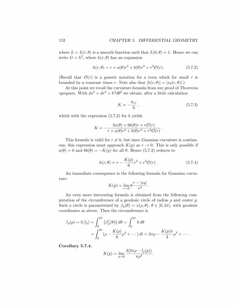
152 CHAPTER 5. DIFFERENTIAL GEOMETRY
where L = L(r, θ) is a smooth function such that L(0, θ) = 1. Hence we canwrite G = h2, where h(r, θ) has an expansion
h(r, θ) = r + a(θ)r2 + b(θ)r3 + r3O(r). (5.7.2)
(Recall that O(r) is a generic notation for a term which for small r isbounded by a constant times r. Note also that |h(r, θ)| = |xθ(r, θ)|.)
At this point we recall the curvature formula from our proof of Theoremaegregium. With ds2 = dr2 + h2dθ2 we obtain, after a little calculation
K = −hrrh, (5.7.3)
which with the expression (5.7.2) for h yields
K = − 2a(θ) + 6b(θ)r + rO(r)
r + a(θ)r2 + b(θ)r3 + r3O(r).
This formula is valid for r 6= 0, but since Gaussian curvature is continu-ous, this expression must approach K(p) as r → 0. This is only possible ifa(θ) = 0 and 6b(θ) = −K(p) for all θ. Hence (5.7.2) reduces to
h(r, θ) = r − K(p)
6r3 + r3O(r) . (5.7.4)
An immediate consequence is the following formula for Gaussian curva-ture:
K(p) = limr→0
6r − |xθ|r3
.
An even more interesting formula is obtained from the following com-putation of the circumference of a geodesic circle of radius ρ and center p.Such a circle is parametrized by βρ(θ) = x(ρ, θ), θ ∈ [0, 2π], with geodesiccoordinates as above. Then the circumference is
lρ(p) = l(βρ) =
∫ 2π
0‖β′ρ(θ)‖ dθ =
∫ 2π
0h dθ
=
∫ 2π
0(ρ− K(p)
6ρ3 + · · · ) dt = 2πρ− K(p)π
3ρ3 + · · · .
Corollary 5.7.4.
K(p) = limρ→0
3(2πρ− lρ(p))πρ3
.

5.7. GEODESIC POLAR COORDINATES 153
Example 5.7.5. A hyperbolic circle of radius ρ has circumference 2π sinh ρ.Hence
K(p) = limρ→0
3(2πρ− 2π sinh ρ)
πρ3= lim
ρ→0
6(ρ− (ρ+ ρ3
6 + · · · ))ρ3
= −1
for every p, as before.
Corollary 5.7.4 also gives an interpretation of the sign of the curvature:K(p) is positive if the circumference of a small geodesic circle is smaller thanthat of a Euclidean circle of the same radius and negative if it is bigger.
Exercise 1 gives a similar result comparing areas of circles.
We now show that geodesic polar coordinates also provide the tools weneed to prove Theorem 5.6.14, in the following form:
Theorem 5.7.6. Every point p in a Riemannian surface S has a neighbor-hood V such that any point q ∈ V − p can be connected to p by a unigueshortest curve, and this curve is a geodesic.
Proof. (We use the same notation as at the beginning of this section.) Letε > 0 such that expp |Bp(ε) is a diffeomorphism, and let V = expp(Bp(ε)).Then any q ∈ V − p can be written as q = x(ρ, θ0) = expp(ρα(θ0)) for aunique ρ ∈ (0, ε) and θ ∈ [0, 2π), and the curve γ(s) = x(s, θ0), s ∈ [0, ρ] isa geodesic of length ρ from p to q.
Let c : [0, a] → S be another curve from p to q. We want to prove thatthe length of c at least ρ. Then we can assume that c(t) 6= p for every t,since otherwise we can replace c with a shorter curve having this property.
Assume first that c([0, a]) ⊂ V . Then we can write c(t) = x(r(t), θ(t)),for uniquely determined functions r : [0, a] → [0, ε) and θ : [0, a] → R,and where r(0) = 0 and r(a) = ρ. Then c′(t) = r′(t)xr + θ′(t)xθ, and|c′(t)|2 = (r′) + (θ′)2h2. For the arclength of c we then have
`(c) =
∫ a
0|c′(t)| dt >
∫ a
0|r′(t)| dt >
∫ a
0r′(t) dt = r(a) = ρ,
with equalities if and only if θ(t) is constant and r(t) is non-decreasing. Butthen c(t) is just a reparametrization of the geodesic γ.
Finally, suppose c is not contained in V . Then there is smallest numbert0 ∈ [0, a] such that c(t0) /∈ V , and the argument above proves that thelength of c|[0, t0] is at least ε, which is bigger than ρ. Hence c must certainlyagain be longer than γ.

154 CHAPTER 5. DIFFERENTIAL GEOMETRY
Exercises for 5.7
1. Let Aρ be the area of a geodesic circle of radius ρ and center p. Provethat
K(p) = limρ→0
12(πρ2 −Aρ)πρ4
.
Use this to give yet another proof that the curvature of the hyperbolicplane is constant equal to −1.
2. Let ds2 = dr2 +G(r, θ)dθ2 be the metric in geodesic polar coordinatesaround the point p ∈ S. Now rescale the metric by a factor λ = c2 asin Exercise 5.4.6, and show that in the new geodesic polar coordinatesthe metric is
ds2 = dr2 + c2G(r
c, θ)dθ2 .
3. Discuss the relationship between formula (5.7.3) and the formula inexercise 5.5.3.
5.8 Riemannian surfaces of constant curvature
We now have the tools necessary for proving one of our main results: thecharacterization of geometries locally isometric to the classical geometries.
Suppose given a function K defined in a neighborhood of p ∈ S. If wewant to find a local Riemannian metric with curvature function K, we haveto find a solution of equation (5.7.3) of the form (5.7.4).
We are interested in the simplest case, namely the case when K is con-stant. Our calculations have shown that surfaces built on the classical ge-ometries have this property, and if you did Exercise 5.5.5, you know thatmetrics obtained from these by scaling have the same property. We want toprove that these are the only ones. This relies on the observation in Propo-sition 5.4.3, saying that if two surfaces can be parametrized by the samesubset of R2 in such a way that the functions E,F and G are the same, thenthey are locally isometric. Thus it suffices to show that a point of a surfaceof constant curvature has a neighborhood such that the metric in geodesicpolar coordinates looks like one of the metrics in Example 5.7.3, possiblyscaled by a constant as in Exercise 5.7.2.

5.8. RIEMANNIAN SURFACES OF CONSTANT CURVATURE 155
So, consider the equation (5.7.3), or equivalently
hrr +Kh = 0, (5.8.1)
for K constant. The general solution of this equation is well known, and wedistinguish between the three cases K = 0, K > 0 and K < 0.
(i) K = 0 : The equation reduces to hrr = 0, which has the solutionsh = Ar+B, where A and B are functions of only θ. But the condition (5.7.4)gives B = 0 og A = 1. Hence the metric has the form ds2 = dr2 + r2dθ2,which is the same as for the Euclidean metric in polar coordinates. Hencea neighborhood of p in S is isometric to a neighborhood of the origin in theEuclidean plane.
(ii) K = 1/R2, R > 0: Equation (5.8.1) is now hrr +1
R2h = 0, with the
general solution
h = A cosr
R+B sin
r
R= A
(1− 1
2
( rR
)2+ · · ·
)+B
(r
R− 1
6
( rR
)3+ · · ·
).
Condition 5.7.4 gives A = 0 and B = R, and the metric becomes
ds2 = dr2 +R2 sin2(r
R) dθ2 .
This is, by Example 5.7.3 and Exercise 5.7.2, the metric on the sphereS2R of radius R. It follows that S must be locally isometric to this sphere.
(iii) K = − 1
ρ2, ρ > 0 : Now (5.8.1) becomes hrr −
1
ρ2h = 0. The general
solution is
h = Aerρ+Be
− rρ = A
(1 +
r
ρ+
1
2
(r
ρ
)2
+ · · ·
)+B
(1− r
ρ+
1
2
(r
ρ
)2
+ · · ·
).
Condition 5.7.4 give A =ρ
2and B = −ρ
2. Consequently, h = ρ sinh
r
ρand
the metric isds2 = dr2 + ρ2 sinh2 r
ρdθ2 . (5.8.2)
But this is the metric of D in geodesic polar coordinates, scaled by theconstant ρ.
Let us denote this scaled version of D by Dρ. We have now proved
Theorem 5.8.1. Suppose S is a Riemannian surfaces such that the Gaus-sian curvature is constant. Then

156 CHAPTER 5. DIFFERENTIAL GEOMETRY
• If K = 0, S is locally isometric to the Euclidean plane.
• If K = 1/R2, S is locally isometric to a sphere of radius R.
• If K = −1/ρ2, S is locally isometric to the hyperbolic plane Dρ.
Remark 5.8.2. Clearly there is a scaled version Hρ as well, and Hρ is iso-metric to Dρ.
Exercises for 5.8
1. Show that G(z) =iz + 1
z + iis an isometry between Hρ and Dρ as Rie-
mannian surfaces for every ρ.
2. Show that if the surface S has a geometric structure modeled on H,then it also has one modeled on Hρ for every ρ > 0.
5.9 The Gauss–Bonnet theorem
Until now, our study of differential geometry has been a study of local prop-erties. In this last section we shall prove the celebrated Gauss–Bonnet the-orem, relating local, geometric information to global, topological propertiesof surfaces. The theorem has a number of striking consequences, and itcan be seen as the first example of an index theorem — a formula relatingtopological and analytic invariants.
Before we state the theorem, we need some more definitions. First, wewill need to define integrals of smooth functions over curves and surfaceregions, generalizing the usual line and surface integrals in R3 to arbitraryRiemannian surfaces.
Line integrals. If f is a function defined on a curve C parametrized by afunction α : [a, b]→ S with ‖α′(t)‖ 6= 0 for all t, we define∫
Cfds =
∫ b
af(α(t))
ds
dtdt =
∫ b
af(α(t))‖α′(t)‖α(t)dt. (5.9.1)

5.9. THE GAUSS–BONNET THEOREM 157
It is not difficult to check that this is independent of the parametrization.If C is only piecewise smooth, we define the integral as the sum of integralsover the smooth pieces.
Surface integrals. Suppose f is defined on a compact region R boundedby a piecewise smooth curve on a Riemannian surface. If R ⊂ x(U) for aparametrization x, we define∫∫
RfdA =
∫∫x−1(R)
f(x(u, v))√EG− F 2dudv. (5.9.2)
By exercise 1. this is independent of choice of parametrizations. If R isnot included in a coordinate neighborhood, we can subdivide it into smallerpieces which are, and define the integral as a sum. This will be independentof the subdivision; cf. the discussion of area in section 5.3. In particular, wecan define the integral over the whole surface S if it is compact.
(These integrals can, of course, also be defined directly as analogues ofRiemann integrals (“limits of sums”). Note also that the formulas for arclength and area in Section 5.3 are special cases.)
The other new ingredient we need is geodesic curvature. Fix a Rieman-nian surface S, and assume that α(s) is a regular curve parametrized by arclength, with unit tangent vector T (s) = α′(s). For every s the curve hastwo possible unit normal vectors nα(s) at α(s). A continuous choice of oneof them we will call a normal orientation of the curve. (Continuous meansthat locally we can write nα = φxu + ψxv, where φ and ψ are continuousfunctions.)
Definition 5.9.1. Let α(s) be a normally oriented curve parametrized byarc length. The geodesic curvature is defined as the normal component ofDα′′(t):
kg(s) = 〈Dα′′(s), nα(s)〉. (5.9.3)
It follows from formula (5.6.3) that for curves on regular surfaces in R3
we haveDα′′(s) = kg(s)nα(s). (5.9.4)
One can show that (5.6.3) holds in general, but we will see that (5.9.4) isalso a consequence of calculations in the proof of Gauss–Bonnet given below.It then follows that the curve is a geodesic if and only if kg(s) = 0 for all s.Hence the function kg can be thought of as a measure of how far the curveis from being a geodesic.
The choice of normal orientation only affects the sign of kg. There aretwo situations where a normal orientation is naturally defined.

158 CHAPTER 5. DIFFERENTIAL GEOMETRY
(i) Usually one considers only the case when the surface S is oriented, andthen the normal vector nα is chosen such that (T (s), nα(s)) is a positivelyoriented (orthonormal) basis for Tα(s)S. For example, if S is a regular surfacein R3 and N is the surface normal defining the orientation, we can setnα(s) = N(α(s))× T (s).
(ii) In the situation we will consider, however, the surface is not neces-sarily oriented, but the curves will all be regular boundary curves of regionsR ⊂ S. Then we can choose nα to be the unit normal vector pointing intoR — i. e. each nα(s) has the form β′(0), for some curve such that β(t) ∈ Rfor t > 0. Note that for this definition of normal orientation, the directionof the boundary curve does not matter.
If R ⊂ S is as in (ii) and S is oriented, the two orientations agree if wechoose to traverse ∂R counterclockwise around R.
Let now S be a connected Riemannian surface, and suppose R ⊂ Sis a compact region bounded by a finite union of regular curves. Denotethe boundary by ∂R. Note that ∂R can have many components, and eachcomponent is a piecewise smooth, closed curve. We are now in situation (ii)above, and each smooth piece is normally oriented by the inward normalvector.
At a non–smooth point pi, R has a well defined interior angle ηi ∈ [0, 2π],and we say that the boundary changes direction by the angle εi = π − ηi ∈[−π, π] at pi. Note that if S is oriented and we follow ∂R counterclockwise,the angle is positive if we turn to the left and negative is we turn to theright.
We call pi a cusp point if εi is ±π. This means that the two smoothboundary curves meeting at pi have the same tangent there.
The Gauss–Bonnet theorem is the following formula:
Theorem 5.9.2. (Gauss–Bonnet)∫∫RKdA+
∫∂Rkgds+
∑i
εi = 2πχ(R). (5.9.5)
Here K and kg are the Gaussian and geodesic curvatures, respectively,and χ(R) is the Euler characteristic of R. (Chapter 3.) The index i runsover all the non–smooth points of ∂R. The striking feature of this formula isthat the left hand side depends entirely on geometric information, whereasthe right hand side is purely topological. For example, If S is compact, wecan apply the theorem to R = S, and the formula simplifies to∫∫
SKdA = 2πχ(S). (5.9.6)

5.9. THE GAUSS–BONNET THEOREM 159
Since the Euler characteristic determines S up to homeomorphism, itfollows that the curvature function also determines S up to homeomorphism!
Here are some more immediate applications:
• For any metric on S2 or P 2 there must be points where the curvatureis positive.
• On orientable surfaces of genus at least 2, there has to be points wherethe curvature is negative.
• On a torus or a Klein bottle the curvature either vanishes everywhere,or it must take both positive and negative values.
In particular, The only compact surfaces that allow metrics of constantpositive curvature are S2 or P 2, the only ones with constant zero curvatureare the torus and the Klein bottle, and neither of these can have metrics ofconstant negative curvature.
These are just a few of the many consequences of the theorem; more willfollow after the proof, which will occupy the next five pages.
Proof of the Gauss–Bonnet theorem. Assume first that no εi is ±π, i. e. ∂Rhas no cusp point. We take as a fact that any such region R can be smoothlytriangulated, i. e. it can be written as a union of smooth, embedded triangles,where the intersection of two distinct triangles (if non–empty) is either acommon side or a vertex. (Cf. Exercise 5.1.10. An embedding is a regular,injective map.) In fact, by further subdividing the triangles, if necessary, wemay assume that every triangle is contained in a normal neighborhood, i. e.a neighborhood parametrized by geodesic polar coordinates, centered at apoint in the interior of some triangle.
We shall see that the general case follows if we can prove the theoremfor each such triangle.
Thus, let R ⊂ Wp be the embedded image of a triangle, where Wp
is parametrized by geodesic coordinates x(r, θ), (r, θ) ∈ [0, ρ) × R, withcenter p = x(0, θ) /∈ ∂R. Although S is not assumed to be orientable, Wp
is, and we now orient it such that (xr, xθ) is a positively oriented basisoutside p. (This orientation extends uniquely also to p, by declaring thate. g. (xr(0, 0), xr(0, π/2)) should be a positively oriented basis there.)
The boundary ∂R is the union of three smooth curves, and we chooseparametrizations by arc length α1(s), α2(s) and α3(s), traversing ∂R incounterclockwise direction, with respect to the orientation chosen on Wp.We may assume that if the length of αi is li, then α1(l1) = α2(0), etc.

160 CHAPTER 5. DIFFERENTIAL GEOMETRY
It also follows that (α′i(li), α′i+1(0)) is a positively oriented basis for
Tαi(li)S = Tαi(li)Vp. Let εi ∈ (0, π) be the angle between α′i(li) and α′i+1(0),where i is counted mod 3. (Cf. also exercise 5.3.5.)
α1
α2
α3
ε1
ε2
ε3
R
Fig. 5.9.1:
We have seen that Gaussian curvature in geodesic polar coordinates is
given by K = −hrrh
, where ds2 = dr2 + h2dθ2 is the metric. Let us now
calculate the geodesic curvature kg for the boundary curves using thesecoordinates.
Write the parametrization of the curve as α(s) = x(r(s), θ(s)). Thenα′ = r′xr + θ′xθ has norm 1. Moreover, ‖xr‖ = 1 and ‖xθ‖ = h, hence α′ =
r′xr + hθ′xθh
is α′ expressed in an orthonormal basis. It follows that there
is an angle φ(s), uniquely determined mod 2π, such that r′(s) = cosφ(s)and hθ′ = sinφ(s). φ(s) is the angle between the geodesic radius throughα(s) and the curve, and it defines a smooth function of s, normalized e. g.by choosing φ(0) ∈ (−π, π]. Moreover, the inward pointing unit normal nαis then determined as
nα = − sinφxr + cosφxθh.
(α′ rotated π/2 in the positive direction.)
The Christoffel symbols for the metric ds2 = dr2 + h2dθ2 are computedfrom equation (5.6.8:
[1 00 h2
] [Γ1
11 Γ112 Γ1
22
Γ211 Γ2
12 Γ222
]=
[0 0 −hhr0 hhr hhθ
].

5.9. THE GAUSS–BONNET THEOREM 161
Formula (5.6.9) for the covariant second derivative now gives:
Dα′′(s) = (r′′ − hhrθ′2)xr + (θ′′ + 2hrhr′θ′ +
hθhθ′
2)xθ
= ((r′)′ − hrθ′(hθ′))xr + ((hθ′)′ + hrr′θ′)
xθh
(5.9.7)
= (− sinφφ′ − hrθ′ sinφ)xr + (cosφφ′ + hrθ′ cosφ)
xθh
= (φ′ + hrθ′)nα(s).
Thus we have the following expression for the geodesic curvature:
kg(s) = φ′ + hrθ′. (5.9.8)
We now compute the integral∫∂Rkgds =
∫∂Rφ′ ds+
∫∂Rhrθ′ds.
(Strictly speaking, we should replace ∂R by the corresponding parameterset on the right hand side, but we choose to simplify the notation, believingthat it is clear what we mean. This remark also applies at several pointslater.)
Consider first the term∫∂R φ
′ds:∫∂Rφ′ds =
∫α1
φ′1ds+
∫α2
φ′2ds+
∫α3
φ′3ds
= (φ1(l1)− φ1(0)) + (φ2(l2)− φ2(0)) + (φ3(l3)− φ3(0)).
The function φi is determined up to a constant multiple of 2π on each αi,uniquely determined by φi(0). If we fix φ1(0), then φ2 and φ3 are determinedby φ2(0) = φ1(l1) + ε1 and φ3(0) = φ2(l2) + ε2. But coming back to α3(l3) =α1(0) we can only say that φ1(0) ≡ φ3(l3) + ε3 (mod 2π). Hence∫
∂Rφ′ds = 2kπ − ε1 − ε2 − ε3
for some integer k.
We state the following result without proof:
Claim: k = 0 if p ∈ intR and k = 1 if p /∈ R. (“Hopf’s Umlaufsatz”.)
This may sound obvious, but the Claim is not at all trivial. Here is anindication of how it can be proved. The idea is to use the fact that k = (
∫∂Rφ′ds+

162 CHAPTER 5. DIFFERENTIAL GEOMETRY
ε1 + ε2 + ε3)/2π is an integer — hence will remain constant under continuousmodifications of the terms involved.
We apply two kinds of such modifications. First consider R as lying in R2 ≈TpS (via exp−1
p ) with the metric ds2 = dr2 + h2dθ2, and deform the metric via
ds2 = dr2 +(tr2 +(1− t))h2dθ2, t ∈ [0, 1] to the standard metric ds2 = dr2 +r2θ2.Then use the fact that ∂R is the boundary of an embedded triangle to deform
to the case where R is a very small Euclidean triangle. (p may remain inside oroutside R throughout this deformation.) But in this situation the claim is easyto verify.
Next we calculate the term∫∂R hrθ
′ds. We must again distinguish be-tween the two cases p /∈ R and p ∈ R — i. e. the case when R is containedin the image of the parametrization x and the case when it is not.
Case 1: p /∈ R. Then Green’s theorem gives∫∂Rhrθ′ds =
∫∂Rhrdθ =
∫∫Rhrrdr dθ =
∫∫R
hrrhh dr dθ = −
∫∫RKdA.
Case 2: p ∈ R. Let Rδ be R minus the interior of a small geodesic disk ofradius δ around p. Then Rδ is contained in the parametrized region, andGreen’s theorem now gives∫
∂Rhrθ′ds = −
∫∫Rδ
KdA+
∫r=δ
hrθ′ds .
Using formula (5.7.2) we see that the last line integral is 2π plus termscontaining the factor δ2. The curvature function K is defined and continuousin all of R. Therefore, taking limits as δ goes to 0, we get∫
∂Rhrθ′ds = −
∫∫RKdA+ 2π.
Putting all this together shows that in both cases we have∫∂Rkgds = 2π −
∫∫RK dA− ε1 − ε2 − ε3,
which completes the proof in the case where R is an embedded triangle con-tained in a normal neighborhood. Note that although we used an auxilliaryorientation of R in the proof, the result is independent of which orientationwe choose, since all the terms can be defined without an orientation.
In the general case (but still no cusp) we can triangulate R as ∪jRj ,where each Rj has this form. Let the interior angles of Rj be ηji = π −

5.9. THE GAUSS–BONNET THEOREM 163
εji, i = 1, 2, 3. Then we can also write Gauss–Bonnet’s theorem for Rj as∫∫Rj
KdA+
∫∂Rj
kgds = ηj1 + ηj2 + ηj3 − π.
Summing over all Rj , we get∫∫RKdA+
∑j
∫∂Rj
kgds =∑j,i
ηji − Tπ , (5.9.9)
where T is the total number of triangles. Denote the three smooth boundarycurves (the “edges”) of Rj by αji, i = 1, 2, 3, all normally oriented by ourconvention. The edges lying in the interior of R will then come in pairs withopposite normal orientations. Hence the geodesic curvatures have oppositesigns, and the corresponding terms cancel in∑
j
∫∂Rj
kgds =∑j,i
∫αji
kgds.
The remaining edges are the ones in ∂R, and we have∑j
∫∂Rj
kgds =∑
αji⊂∂R
∫αji
kgds =
∫∂Rkgds.
It remains to analyze the right hand side of (5.9.9). Observe first that thesum of all the angles ηji around an internal vertex of R is 2π, so summingall such angles, we get 2π(V − V∂), where V and V∂ denote the numbers ofvertices in R and ∂R.
The remaining angles ηji are interior angles at vertices in ∂R. Note thateach non–smooth point must be such a vertex, and there the angles sum upto π − εk, where this defines the external angle εk ∈ (−π, π) at this vertex.At each smooth point the angles ηji sum up to π.
It follows that the sum of all ηji at all vertices in ∂R is V∂ π −∑k
εk.
Let E be the total number of edges in R and E∂ the number of edges in∂R. Then clearly
E∂ = V∂ .
Since every triangle has three edges, of which interior edges lie in twotriangles and boundary edges lie in one, we also have the relation
3T = 2E − E∂ .
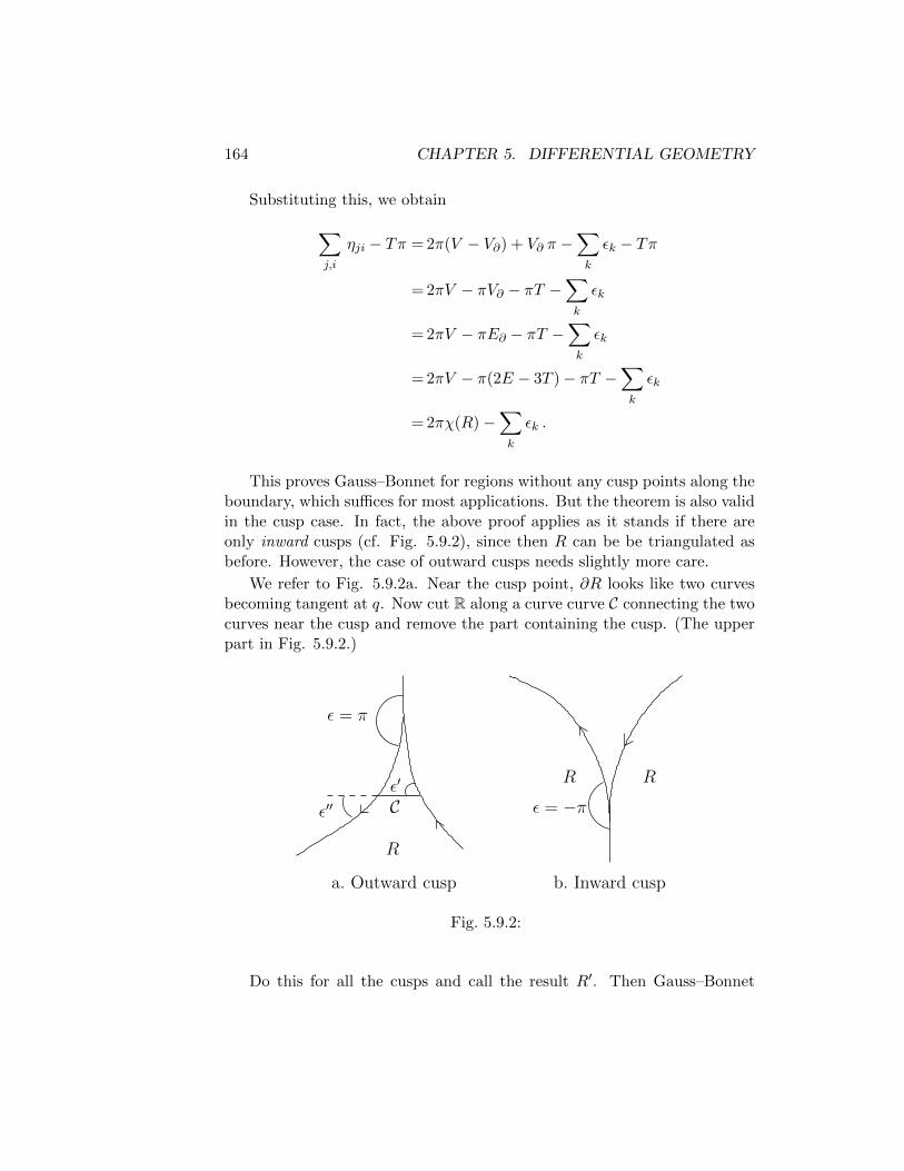
164 CHAPTER 5. DIFFERENTIAL GEOMETRY
Substituting this, we obtain∑j,i
ηji − Tπ = 2π(V − V∂) + V∂ π −∑k
εk − Tπ
= 2πV − πV∂ − πT −∑k
εk
= 2πV − πE∂ − πT −∑k
εk
= 2πV − π(2E − 3T )− πT −∑k
εk
= 2πχ(R)−∑k
εk .
This proves Gauss–Bonnet for regions without any cusp points along theboundary, which suffices for most applications. But the theorem is also validin the cusp case. In fact, the above proof applies as it stands if there areonly inward cusps (cf. Fig. 5.9.2), since then R can be be triangulated asbefore. However, the case of outward cusps needs slightly more care.
We refer to Fig. 5.9.2a. Near the cusp point, ∂R looks like two curvesbecoming tangent at q. Now cut R along a curve curve C connecting the twocurves near the cusp and remove the part containing the cusp. (The upperpart in Fig. 5.9.2.)
R Rε′
ε = π
ε = −π
a. Outward cusp b. Inward cusp
ε′′
R
C
Fig. 5.9.2:
Do this for all the cusps and call the result R′. Then Gauss–Bonnet

5.9. THE GAUSS–BONNET THEOREM 165
applies to R′, to give∫R′KdA+
∫∂R′
kgds = 2πχ(R′)−∑i∈Io
εi −∑j∈Ic
(ε′j + ε′′j ) ,
where the index set Ic corresponds to the outward cusp points and Io to theother corners. For each cusp point ∂R′ has two corners with angles ε′ andε′′, and as we let the curve C move toward the cusp point, we can arrangefor the sum ε′ + ε′′ to tend to π. In the limit we get formula (5.9.5), wherenow εi = π.
We end with some more examples of applications of the Gauss–Bonnettheorem.
(1) Area formulas for geodesic triangles:
Let R be a triangle with geodesic sides and interior angles α, β and γ.Then
∫∫RKdA = α+ β + γ − π. If K is constant, we get
KA(R) = α+ β + γ − π ,
which gives the well–known area formulas in hyperbolic and spherical geom-etry. In Euclidean geometry it reduces to the relation α+ β + γ = π.
(2) A closed geodesic cannot bound a disk on a surface with curvatureless than or equal to 0. For along such a curve kg = 0, so if it bounds aregion R homeomorphic to a disk, we would have
∫∫RKdA = 2π− ε, where
ε ≤ π. But then K cannot be non-positive on R.
(3) Similarly, on a surface of curvature ≤ 0 two geodesics cannot meetat two points so as to bound a region R homeomorphic to a disk, becausewe then would have
∫∫RKdA = 2π − ε1 − ε2 for two angles εi < π. This
means, for example, that in a neighborhood parametrized by a disk, therecan be only one geodesic joining two points.
(4) Two simple, closed geodesics on a compact surface S of everywherepositive curvature must have a point of intersection.
In fact, by Gauss–Bonnet, χ(S) > 0, so S ≈ S2. If γ1 and γ2 are twogeodesics which do not intersect, they must bound a region R ≈ S1 × I,which has Euler characteristic 0. Hence 0 = 2πχ(R) =
∫∫RK > 0, which is
a contradiction.
(5) As an example of a completely different kind of application we get anew proof that the Euler characteristic is independent of triangulation. Notethat there is no relation at all between triangulations and metrics locally.

166 CHAPTER 5. DIFFERENTIAL GEOMETRY
Exercises for 5.9
1. Show that the definition of surface integrals is independent of choiceof parametrization. (Use Exercise 5.3.4.)
2. Find a formula for the geodesic curvature in terms of a parametrizationβ(t) which is not necessarily by arc length.
3. Verify “Hopf’s Umlaufsatz” for a Euclidean triangle in R2.
4. Generalize the area formulas in the constant curvature cases to arbi-trary geodesic n–gons.
5. Show that a compact, oriented Riemannian surface S with curvatureeverywhere 0 is homeomorphic to a torus.
Show that if K ≥ 0, but not 0 everywhere, then S is homeomorphicto a sphere.
6. Suppose S is a compact, oriented surface with constant curvature K 6=0, and suppose that S = S1 ∪ S2, where S1 ∩ S2 is a simple, closed,geodesic. Show that the ratio between the areas of S1 and S2 is arational number.
What is this number if K > 0?
7. Assume that a surface homeomorphic to T 2#T 2#T 2 has a geometricstructure modeled on standard hyperbolic geometry. What is its area?
8. Use the Gauss–Bonnet theorem to compute the geodesic curvature ofcircles on the standard S2.
9. Let C be a hyperbolic circle of (hyperbolic) radius ρ. Explain why thegeodesic curvature kg of C is constant and depends only on ρ.
Compute kg.
10. Let p be a point in a Riemannian surface S. Let εn be a sequence ofpositive numbers converging to 0, and let Cn be a sequence of simpleclosed curves with no non-smooth points, such that d(q, p) < εn forevery q ∈ Cn. Prove that
limn→∞
∫Cnkgds = 2π.
11. Verify the claim in Remark 4.2.2.

5.9. THE GAUSS–BONNET THEOREM 167
12. Let P ⊂ R3 be a polyhedron homeomorphic to a compact surface. Ifv is a vertex P , define its defect d(v) to be 2π − α(v), where α(v)is the sum of the angles around v. (Hence d(v) measures the failureof P to lie in a plane near v.) Define the total defect of P to beD(P ) = Σvd(v), where the sum is over all the vertices of P .
Show that D(P ) = 2πχ(P ). (Descartes’ theorem.)

168 CHAPTER 5. DIFFERENTIAL GEOMETRY

Index
E(2), 19
PGL2(C), 22
PSL2(R), 24
[z, z1, z2, z3], 23
B, 13, 77
C, C–circles, 19
D, 17, 49
Γkij , 141
H, 18, 39
K, 13, 73
R, 19
AD, 63
AH, 61
χ(M), 90
dD, 53
dH, 52
dK, 73
expp, 145
kg, 157
Mob(±)(C), 21, 24
Mob(±)(D), 50
Mob(±)(H), 24, 25
angle, 4
arc–length
hyperbolic, 56
on surfaces, 117
area
hyperbolic, 61, 63
on surfaces, 119
asymptotic triangle, 62
axiomsArchimedes, 7betweenness, 3congruence, 5continuity, 7Dedekind, 7incidence, 2parallel
Euclidean, 7hyperbolic, 12
Pasch, 3Playfair, 7
Beltrami–Klein model K, 12, 73Brioschi’s formula, 131
chain rule, 109Christoffel symbols, 141conformal
equivalence, 119map, 21, 125model, 49
congruence criteria, 6, 69, 70connected sum, 82coordinate transformation, 105coordinate transformations, 94cosine law, hyperbolic, 67, 68covariant second derivative, 138cross–ratio, 23curvature
Gaussian, 126geodesic, 157
169

170 INDEX
mean, 136principal, 136
cusp point, 158
derivative, 108differentiable structure, 94
elliptic type, 30Erlangen program, 100Euclidean group, 6, 19Euclidean structure, 95Euler characteristic, 90exponential map, 145
first fundamental form, 118FLT; fractional linear transforma-
tions, 20
Gauss map, 126Gauss’ lemma, 150Gauss–Bonnet Theorem, 158genus, 91geodesic
circle, 149curve, 138polar coordinates, 149radius, 149
geodesically complete, 146geometric structure, 95
Hopf’s Umlaufsatz, 161Hopf–Rinow theorem, 146hyperbolic structure, 97hyperbolic type, 30hyperboloid model, 78
ideal vertex, 62incidence geometry, 2intrinsic, 123inversion, 35isometry, 121
Isothermal coordinates, 125
Klein bottle, 84
line integral, 156Lorentz group, 79
Mobius band, 85Mobius transformations, 19
normal form, 34normal neighborhood, 146normal orientation, 157
orientation, 85, 113
parabolic type, 30parametrization, 105Poincare upper half–plane H, 17Poincare’s disk model D, 17Poincare’s disk model D, 49projective plane, 3, 82pseudosphere, 124Pythagorean theorem, 67
ray, 4regular surface, 107Riemann sphere, 19Riemannian metric, 117
segment, 4sine law, hyperbolic, 68spherical geometry, 2spherical structure, 97Stereographic projection, 13surface, 81surface integral, 157
tangent plane, 107Theorema egregium, 130torus, 82triangle, 2