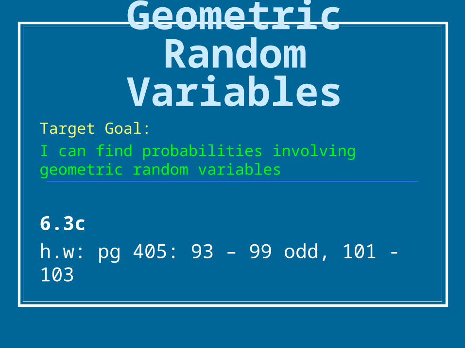
Geometric Random Variables

Target Goal:

I can find probabilities involving geometric random variables

6.3c

h.w: pg 405: 93 – 99 odd, 101 - 103

Review Binomial: The # of trials n is fixed. X counts the number of successes. Possible values of X are 0, 1, 2…, n Probability for success same for all n Independence

Consider: Flip a coin until you get a head. Roll a die until you get a 3. Shoot three pointers until you make 1.

What is the main difference?

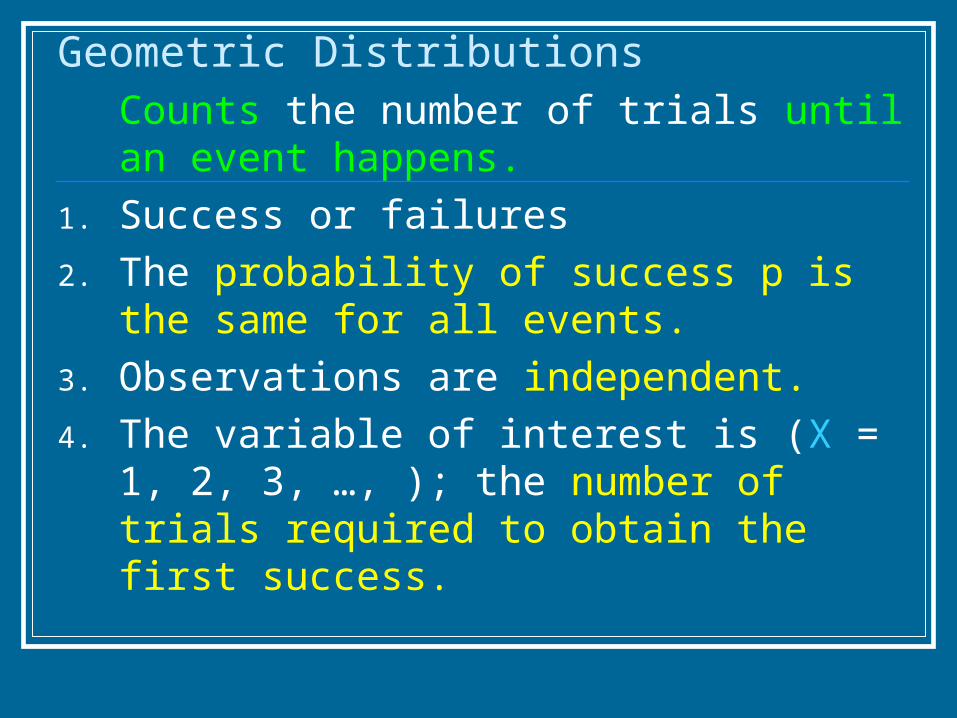
Geometric Distributions

Counts the number of trials until an event happens.

1. Success or failures

2. The probability of success p is the same for all events.

3. Observations are independent.

4. The variable of interest is (X = 1, 2, 3, …, ); the number of trials required to obtain the first success.

What does represent?

You will never get a success loser.

Which is a Geometric Distribution? Check the conditions.

Roll Die until “3”Roll Die until “3” Draw an Ace Draw an Ace

Success or Success or failuresfailures

The prob. same The prob. same for all eventsfor all events

Observations Observations are independent are independent

Execute until Execute until event occurs? event occurs?

YY YY

YY

YY YY

Y:1/6Y:1/6 N: First draw: 4/52N: First draw: 4/522nd draw: 4/51 2nd draw: 4/51

N: previous pick effectsN: previous pick effects the next.the next.

Rules for Calculating Geometric Probabilities

The probability of the first success on the nth trial is:P(X=n) = (1-p)n-1p for X = 1, 2, 3, …..

{s/a qn-1p}

((1-p) s/a 1-p) s/a q: Probability of failure q: Probability of failure withwithp being the probability of successp being the probability of success

Note:

The longer it takes to get the first success, the closer the probability gets to 0.

The table of probabilities could have no end.

Example: Roll a DieConstruct the probability distribution table for X= the number of rolls of a die until a three occurs.

P(X=1) = (5/6)0(1/6)1 = 0.1667 P(X=2) = (5/6)1(1/6)1 = P(X=3) = P(X=4) =

Complete and fill in table.

P(X=n) = (1-p)P(X=n) = (1-p)n-1n-1pp

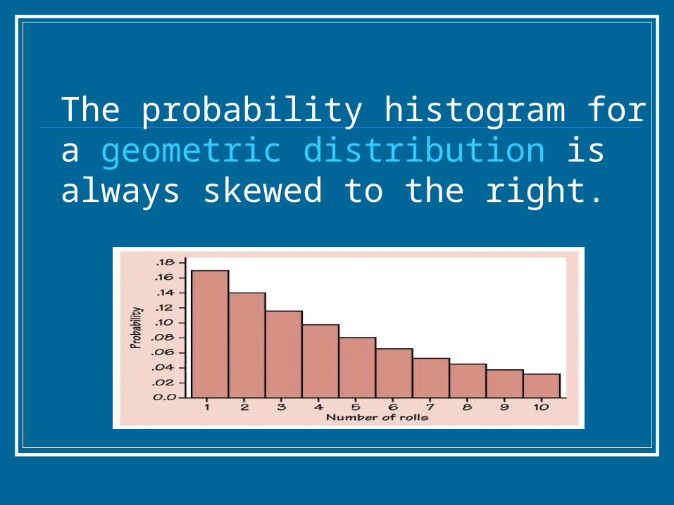
The probability histogram for a geometric distribution is always skewed to the right.

Exercise: Hard Drive

Suppose we have data that suggest that 3% of a company’s hard drives are defective.

You have been asked to determine the probability that the first defective hard drive is the fifth unit tested.

a) Verify that this is a geometric setting.

Success or failures? The prob. same for all events? Observations are independent? Execute until event occurs?

Identify the random variable: X = number of drives tested in order to find

the first defective

What constitutes success in this situation? Success is a defective hard drive.

b) What is the probability that the first defective hard drive is the fifth unit tested?

P(X=5) = (1-0.03)5-1 (.03)

= (0.97)4(.03)

= .0266

P(X=n) = (1-p)P(X=n) = (1-p)n-1n-1pp

c) Find the first four entries in the table of the pdf for the random variable X.

XX 11 22 33 44

P(X) P(X) .03.03 .0291.0291 .0282.0282 .0274.0274

P(X=1), P(X=2), etcP(X=1), P(X=2), etc. (2min)

Mean or Expected Value

The Mean or Expected Value of a geometric variable is:

The Variance of X is:

σ2 = (1-p)/p2

σ =

x

1=p

2/ pq

The probability that it takes more than n trails to see the first success is:

P(X>n) = (1-p)n or qn

Ex. Roll a die until a 3 is observed. The probability that it takes more than 6

rolls to observe a 3 is:

P(X>6) = (1-p)n

= (5/6)6

0.335

Exploring Geometric Distributions: Calculator

Verify our previous results. Enter the list of the # of trials, 1 to 7 in L1.

Highlight L2 and enter geometric pdf’s;

Select 2nd VARS: geometpdf (1/6,L1): Enter

Plot Histogram on Plot1 Set windows to X[0,11]1 and Y[-.05, .2]0.1

Xlist: L1, freq: L2 Trace

Enter geometcdf as L3

Highlight L3

Select 2nd VARS: geometcdf (1/6,L1): Enter

Plot the Cumulative Distribution Histogram.

Deselect Plot 1, select plot2 Xlist: L1, freq: L3 Windows: X[0,11]1 and Y[-.3, 1].1

Trace

Simulating Geometric Experiments

Called “wait time” because you continue to conduct trails until a success is observed.

Example : Show me the Money! Cheerios claims a free $1 bill every 20th

box. Let’s simulate to determine how many

boxes you need to buy to get the money.

Simulation with Table D Let 2 digit numbers 00 to 99 represent a

box of Cheerios. Let 01 to 05 represent a box with $1. Let 00, 06 to 99 represent a box w/o $1 Read Table B, line 127:

Form pairs and organize into 5 rows, ten across until a 01 to 05 is found.

Ex. 23 33 06 …

How many boxes did it take?

Why?

55!55!

Check the variationCheck the variation..

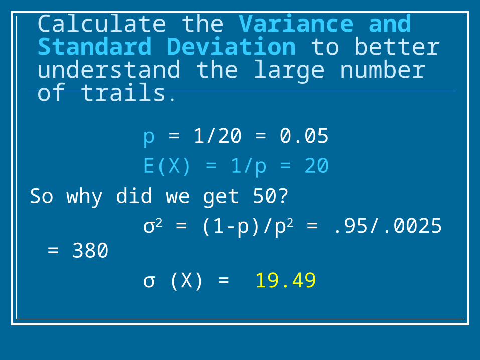
Calculate the Variance and Standard Deviation to better understand the large number of trails.

p = 1/20 = 0.05

E(X) = 1/p = 20

So why did we get 50?

σ2 = (1-p)/p2 = .95/.0025 = 380

σ (X) = 19.49

How many standard deviations is our result from the mean?

55 is about 1.8 σ’s to the right of the mean 20. (35 away from 20)

So it is reasonable.

Recall:

σ is not an appropriate measure of spread for strongly skewed distributions.

Our geometric distribution is strongly skewed right.