Geometric Approach to Solving the Inverse … · Ce qui est nécessaire c’est uniquement le...

GEOMETRIC APPROACH TO SOLVING THE INVERSE DISPLACEMENT PROBLEM OFCALIBRATED DECOUPLED 6R SERIAL ROBOTS

Albert Nubiola and Ilian A. BonevDepartment of Automated Manufacturing Engineering, École de Technologie Supérieure, Montreal, QC, Canada

E-mail: [email protected]

Received March 2013, Accepted January 2014No. 13-CSME-118, E.I.C. Accession 3576

ABSTRACTThis paper presents a simple but efficient way to numerically calculate the inverse displacement problem ofcalibrated decoupled 6R serial robots. The method is iterative and works with any type of calibrated robotmodel, such as level-3 models, since it requires no algebraic computation and no resolution of high-orderpolynomials, only the computation of the forward displacement problem of the calibrated robot model andthe inverse kinematics of the nominal robot model. The method proposed can find up to eight possiblesolutions for a given end-effector pose. A numerical example is presented, with one million arbitrary end-effector poses of a level-3 calibrated ABB IRB 120 robot. The computation time for solving the inverseproblem is analyzed, and in most cases is found to be only four times the time needed to calculate thenominal inverse kinematics and the calibrated direct kinematics. Furthermore, the method is fast enough tobe implemented directly into the robot controller using the RAPID programming language.

Keywords: inverse kinematics; decoupled serial robot; robot calibration.

APPROCHE GÉOMÉTRIQUE POUR RÉSOUDRE LA CINÉMATIQUE INVERSEDES ROBOTS SÉRIELS 6R DECOUPLÉS

RÉSUMÉCet article présente une méthode simple et efficace pour calculer la cinématique inverse des robots sériels 6Rdécouplés. La méthode est itérative et fonctionne pour tous les modèles théoriques de robots étalonnés (parexemple, des modèles du niveau 3), étant donné qu’aucun calcul algébrique ou résolution des polynômesd’ordre élevé n’est nécessaire. Ce qui est nécessaire c’est uniquement le calcul de la cinématique directe durobot étalonné et la résolution de la cinématique inverse du modle nominal du robot. La méthode proposéepeut trouver jusqu’à huit solutions possibles pour une pose de l’effecteur. Un exemple numérique est montréincluant un million de poses arbitraires pour l’effecteur d’un robot ABB IRB 120 étalonné (étalonnage duniveau 3). Le temps de calcul nécessaire pour résoudre la cinématique inverse est analysé ; dans la plupartdes cas on trouve qu’il est quatre fois le temps nécessaire pour calculer la cinématique inverse nominale etla cinématique directe du modèle étalonné. En plus, cette méthode est assez rapide pour être implémentéedans le contrôleur du robot en utilisant le langage de programmation RAPID.

Mots-clés : cinématique inverse ; robot sériel découplé ; étalonnage de robots.

Transactions of the Canadian Society for Mechanical Engineering, Vol. 38, No. 1, 2014 31

1. INTRODUCTION

Solving the inverse kinematics of a decoupled 6R serial robot is relatively straightforward, and is generallyachieved using analytical methods [1, 2] (closed-form solution). However, solving the inverse displacementproblem (IDP) of such a robot when calibrated with a so-called level-2 model (only geometric errors con-sidered) or, even worse, a level-3 model (where non-geometric errors are also considered), is much morecomplicated, and requires numerical methods [3–6].

It is well known that up to sixteen solutions can be found by solving the IDP of a general 6R serialrobot. However, such a complete solution requires substantial computing time [7, 8] and is not suitablefor real-time computation. As a result, researchers usually prefer to use practical numerical approaches[9]. Ways to efficiently calculate the IDP have improved considerably since the first attempts to solve theIDP [10]; however, the most recent works [11, 12] still require the solution of a univariate polynomial ofdegree 16.

An example of level-2 calibration is given in [13], where a camera is mounted on the robot to perform aclosed-loop calibration. Unfortunately, the authors do not mention how they solve the IDP. It becomes evenmore complicated for level-3 models, due to the presence of non geometric parameters, such as compliancecoefficients or thermal expansion coefficients. Depending on the complexity of such a model, a numericalmethod might often be the only way of solving the inverse problem.

Numerical methods can be divided into three types [5]: (1) Newton–Raphson methods, (2) predictor-corrector type algorithms, and (3) optimization techniques using the formulation of a scalar cost function.Examples of the first type can be found in [14], where a modified Newton-Gauss method is used. Thesemethods involve the computation of the Jacobian matrix. A comparison between Newton–Raphson methodsand predictor-corrector-type algorithms is provided in [15], where the authors conclude that the latter arefaster.

An example of a predictor-corrector algorithm is given in [16]. This type of method often requires a largenumber of iterations, and does not always converge. Some of these algorithms also require computationof the Jacobian matrix, like the algorithm proposed in [17], which combines a predictor-corrector type ofalgorithm with a least-squares optimization technique, or the closed-loop method [6] where the inversekinematic problem is solved as a control problem for a simple dynamic system. However, optimizationtechniques are usually complex, and several iterations are needed to achieve a solution.

Two approaches for level-2 calibrations are proposed in [4] using the nominal inverse kinematics. How-ever, the solution becomes complex when the number of error parameters increases. The resolution of anonlinear programming problem is divided into two phases in [18] for greater efficiency.

Finally, [5] greatly reduced the amount of computing time needed to solve the inverse problem, by calcu-lating a so-called pose shift by iteratively adding and subtracting computed poses based on a truncated-seriesexpansion of the desired pose. However, we realized that their method could be further improved by usingpose multiplications based on a geometric principle, instead of adding and subtracting the poses of thetruncated-series expansion of the desired pose.

This paper presents a new type of numerical solution: a geometrical and iterative method which incre-mentally approaches the final solution at each iteration. Like the method proposed in [5], our method doesnot need computation of the Jacobian matrix or derivatives of any kind. From the sixteen possible solu-tions to the IDP of the calibrated robot, up to eight can be obtained, and the new method only needs theforward displacement model of the calibrated robot model and the nominal inverse kinematics solution ofthe nominal robot model.

Although our iterative method works with any decoupled 6R serial robot and any calibration model, ournumerical example is based on an ABB IRB 120 robot calibrated using a typical level-3 model. Thesemodels are presented in Section 2. The method proposed for solving the inverse problem is then detailed in

32 Transactions of the Canadian Society for Mechanical Engineering, Vol. 38, No. 1, 2014

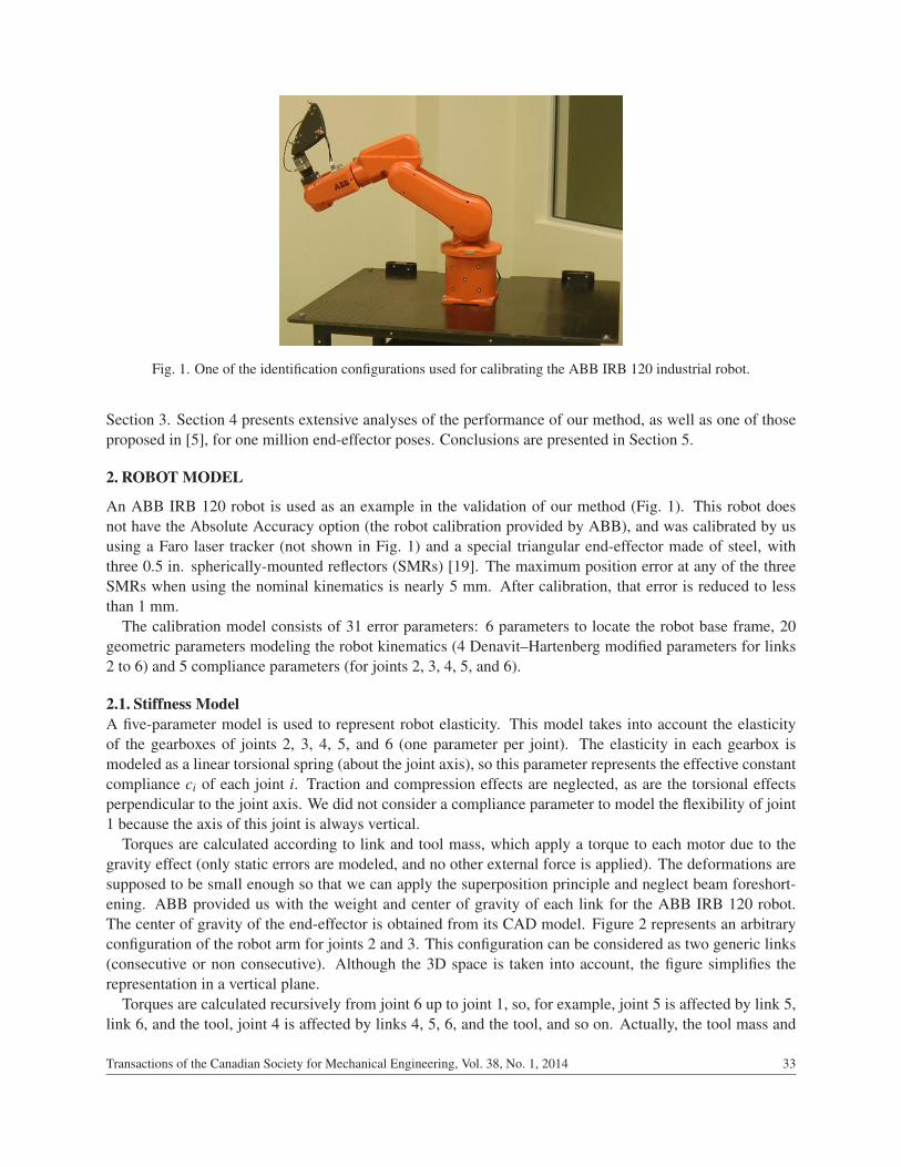
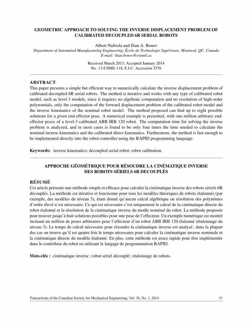
Fig. 1. One of the identification configurations used for calibrating the ABB IRB 120 industrial robot.

Section 3. Section 4 presents extensive analyses of the performance of our method, as well as one of thoseproposed in [5], for one million end-effector poses. Conclusions are presented in Section 5.

2. ROBOT MODEL

An ABB IRB 120 robot is used as an example in the validation of our method (Fig. 1). This robot doesnot have the Absolute Accuracy option (the robot calibration provided by ABB), and was calibrated by ususing a Faro laser tracker (not shown in Fig. 1) and a special triangular end-effector made of steel, withthree 0.5 in. spherically-mounted reflectors (SMRs) [19]. The maximum position error at any of the threeSMRs when using the nominal kinematics is nearly 5 mm. After calibration, that error is reduced to lessthan 1 mm.

The calibration model consists of 31 error parameters: 6 parameters to locate the robot base frame, 20geometric parameters modeling the robot kinematics (4 Denavit–Hartenberg modified parameters for links2 to 6) and 5 compliance parameters (for joints 2, 3, 4, 5, and 6).

2.1. Stiffness ModelA five-parameter model is used to represent robot elasticity. This model takes into account the elasticityof the gearboxes of joints 2, 3, 4, 5, and 6 (one parameter per joint). The elasticity in each gearbox ismodeled as a linear torsional spring (about the joint axis), so this parameter represents the effective constantcompliance ci of each joint i. Traction and compression effects are neglected, as are the torsional effectsperpendicular to the joint axis. We did not consider a compliance parameter to model the flexibility of joint1 because the axis of this joint is always vertical.

Torques are calculated according to link and tool mass, which apply a torque to each motor due to thegravity effect (only static errors are modeled, and no other external force is applied). The deformations aresupposed to be small enough so that we can apply the superposition principle and neglect beam foreshort-ening. ABB provided us with the weight and center of gravity of each link for the ABB IRB 120 robot.The center of gravity of the end-effector is obtained from its CAD model. Figure 2 represents an arbitraryconfiguration of the robot arm for joints 2 and 3. This configuration can be considered as two generic links(consecutive or non consecutive). Although the 3D space is taken into account, the figure simplifies therepresentation in a vertical plane.

Torques are calculated recursively from joint 6 up to joint 1, so, for example, joint 5 is affected by link 5,link 6, and the tool, joint 4 is affected by links 4, 5, 6, and the tool, and so on. Actually, the tool mass and


Fig. 2. Schematics of two consecutive links under the gravity effect.

its center of gravity can be combined with link 6, as they do not move with respect to one another, and sothis recursive method already includes the tool.

The gravity vector seen by joint i corresponds to

gi = (H0i )

−1g0, (1)

whereHa

b = Aaa+1 Aa+1

a+2 . . . Ab−1b , (2)

if b > a. Then, the gravity force of link j seen by link i can be found as

fij = m jgi = m j(H0

i )−1g0 = [ f i

x, f iy, f i

z ,1]. (3)

We can also find the center of gravity of link j with respect to the coordinates of frame i, cij if we know

the center of gravity of link j with respect to the local coordinates, c j

cij = Hi

jc j = [cix, j,c

iy, j,c

iz, j,1]

T , (4)

where Hij is the identity matrix if i = j.

Once we have calculated all the combinations where i ≤ j, we can calculate the torque supported by eachjoint

τi = τi,linki + τi,link,i+1 + · · ·+ τi,link6, (5)

where τi,link j is the contribution of the torque supported by joint i caused by link j

τi,link j = f iy, jc

ix, j − f i

x, jciy, j . (6)

In our case, we took into account the gravity forces due to the masses of links 2, 3, 4, and the tool. Weneglected the masses of links 5 and 6, as they are relatively small.


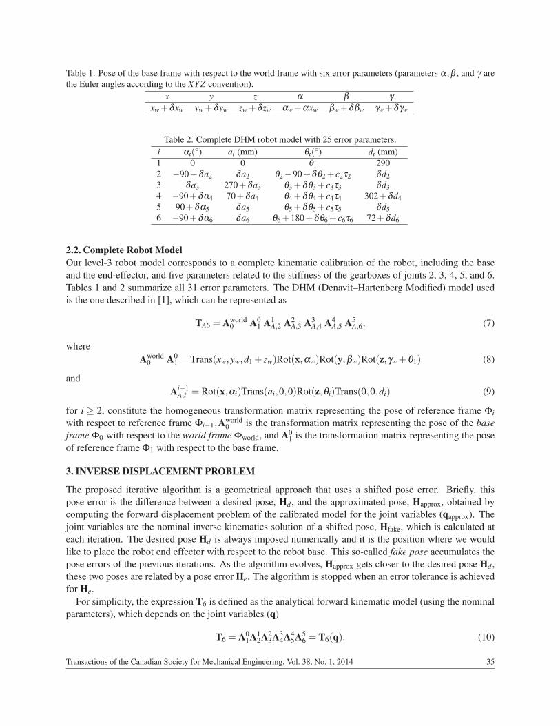
Table 1. Pose of the base frame with respect to the world frame with six error parameters (parameters α,β , and γ arethe Euler angles according to the XY Z convention).

x y z α β γ

xw +δxw yw +δyw zw +δ zw αw +αxw βw +δβw γw +δγw

Table 2. Complete DHM robot model with 25 error parameters.i αi(

◦) ai (mm) θi(◦) di (mm)

1 0 0 θ1 2902 −90+δa2 δa2 θ2 −90+δθ2 + c2τ2 δd23 δa3 270+δa3 θ3 +δθ3 + c3τ3 δd34 −90+δα4 70+δa4 θ4 +δθ4 + c4τ4 302+δd45 90+δα5 δa5 θ5 +δθ5 + c5τ5 δd56 −90+δα6 δa6 θ6 +180+δθ6 + c6τ6 72+δd6

2.2. Complete Robot ModelOur level-3 robot model corresponds to a complete kinematic calibration of the robot, including the baseand the end-effector, and five parameters related to the stiffness of the gearboxes of joints 2, 3, 4, 5, and 6.Tables 1 and 2 summarize all 31 error parameters. The DHM (Denavit–Hartenberg Modified) model usedis the one described in [1], which can be represented as

TA6 = Aworld0 A0

1 A1A,2 A2

A,3 A3A,4 A4

A,5 A5A,6, (7)

whereAworld

0 A01 = Trans(xw,yw,d1 + zw)Rot(x,αw)Rot(y,βw)Rot(z,γw +θ1) (8)

andAi−1

A,i = Rot(x,αi)Trans(ai,0,0)Rot(z,θi)Trans(0,0,di) (9)

for i ≥ 2, constitute the homogeneous transformation matrix representing the pose of reference frame Φi

with respect to reference frame Φi−1,Aworld0 is the transformation matrix representing the pose of the base

frame Φ0 with respect to the world frame Φworld, and A01 is the transformation matrix representing the pose

of reference frame Φ1 with respect to the base frame.

3. INVERSE DISPLACEMENT PROBLEM

The proposed iterative algorithm is a geometrical approach that uses a shifted pose error. Briefly, thispose error is the difference between a desired pose, Hd , and the approximated pose, Happrox, obtained bycomputing the forward displacement problem of the calibrated model for the joint variables (qapprox). Thejoint variables are the nominal inverse kinematics solution of a shifted pose, Hfake, which is calculated ateach iteration. The desired pose Hd is always imposed numerically and it is the position where we wouldlike to place the robot end effector with respect to the robot base. This so-called fake pose accumulates thepose errors of the previous iterations. As the algorithm evolves, Happrox gets closer to the desired pose Hd ,these two poses are related by a pose error He. The algorithm is stopped when an error tolerance is achievedfor He.

For simplicity, the expression T6 is defined as the analytical forward kinematic model (using the nominalparameters), which depends on the joint variables (q)

T6 = A01A1

2A23A3

4A45A5

6 = T6(q). (10)


Defining TA6 as the forward displacement model of the calibrated robot (where the index A stands for “ac-tual”, closer to the real behavior), which depends on the joint variables, q, and the identified error parameters,we have once again

TA6 = Aworld0 A0

1A1A,2A2

A,3A3A,4A4

A,5A5A,6 = TA6(q). (11)

If we want to find the inverse solution for a desired pose Hd , which represents the pose of frame 6 withrespect to the robot base frame, we must proceed with the following steps of the iteration k:

A. Set k = 1.

B. Calculate the vector of joint variables qapprox,1, by solving the inverse kinematics of the nominal robotmodel at pose Hd [1–2] (see appendix).

C. Calculate the first pose shift as Happrox,k = TA6(qapprox,k).

D. If the error between Happrox,k and Hd is smaller than the tolerance error, we take qapprox,k as the jointsolution of the calibrated model for Hd ; otherwise, we increase k and we continue with the followingsteps.

E. Calculate the fake pose using the following equation (Hfake,1 = Hd)

Hfake,k = Hfake,k−1(Happrox,k−1)−1Hd (12)

F. Find the vector qapprox,k using the nominal robot model, i.e. using the algebraic inverse kinematicssolution [1–2] for Hfake,k (closed-form solution).

G. Go back to step C.

The block diagram of this algorithm is shown in Fig. 3, where IK stands for the inverse kinematics of thenominal robot model. Figure 4 illustrates the iterative approach for iteration k.

The core of the algorithm remains in step E, which calculates the fake pose that will find a better config-uration of the robot joints at every iteration. This method differs from [5] in that the fake pose is calculatedusing matrix multiplications instead of additions. The main advantage is that a pure homogenous pose isobtained as a result. Referring to Fig. 4, we can see the geometric principle of the algorithm: the fake poseHfake,k+1 is obtained as the pose shift between the desired pose Hd and the approximate pose Happrox,k, addedto the fake pose of the previous iteration Hfake,k. Figure 4 could be seen as the second iteration (for the firstiteration Hfake,1 = Hd).

The error between Happrox,k and Hd takes into account the position error and the orientation error, and isdefined in [20] (first and second term respectively)

E =√

x2e + y2

e + z2e + pcos−1

(re1,1 + re2,2 + r−1

e3,3

2

), (13)

where xe,ye, and ze are the components of the position error and re1,1,re2,2, and re3,3 are the diagonal elementsof the rotation matrix representing the orientation error. Note that for iteration k, the pose error is

He,k = Hd(Happrox,k)−1 =

re1,1 re1,2 re1,3 xe

re2,1 re2,2 re2,3 ye

re3,1 re3,2 re3,3 ze

0 0 0 1

. (14)


Fig. 3. Block diagram for the proposed algorithm.

Fig. 4. Iterative representation for iteration k.


Finally, we used p = (180/π) mm/◦ for our tests, so that the same importance is attributed to both 1 mmand 1◦ (cos−1 returns the angle in radians).

For some robot configurations, it can happen that the algorithm does not behave as expected. For example,there may be no solution after a certain number of iterations because we are too close to an elbow singularity.In the results section, we tagged these configurations as “unstable” and their behavior is studied in detail.A robot configuration is considered to be unstable if any of the three following conditions apply: (1) theresulting assembly mode for any iteration is different than the desired one (i.e., elbow-up vs. elbow-down),(2) the error increases or (3) the algorithm reaches ten iterations.

4. RESULTS

To experimentally test convergence, we used one million end-effector poses to numerically compute theinverse solution of our calibrated ABB IRB 120 industrial robot. Each end-effector pose is calculated by arandom configuration of robot joints. The random configurations are equally distributed in the joint space,which means that for every configuration, a random joint angle set is chosen between the robot joint limits.The real robot is not used anytime to perform this tests. From each configuration, the modified forwardkinematics is calculated obtaining a pose. Our inverse algorithm is applied to each of these poses. The goalis to obtain the joints that were used to generate every pose, so the final configuration must be the same. Thealgorithm can find up to eight solutions, however, it would take eight times longer to compute with respectto the presented results (the final configuration must be chosen after the first iteration).

It is important to note that, although it might appear that we deliberately chose a small robot to test ourmethod, this particular robot is actually less accurate (before calibration) than a much larger industrial robot.Indeed, the ABB IRB 120 robot presented a maximum position error of about 5 mm before calibration. Thiserror was reduced to less than 1 mm after calibration.

Our algorithm was implemented in MATLAB using mex functions to improve the algorithm speed. Al-though MATLAB is known to be relatively slow, our goal was not to obtain the solution as quick as possible,but to evaluate its convergence and find the average number of iterations needed to reach the solution for agiven tolerance. MATLAB’s profile function was used to track the time spent on each task.

We computed a maximum of 10 iterations for each of the end-effector pose. The position and orientationerrors were stored for each iteration. Other information regarding the stability of our algorithm was alsostored.

To decide when to stop iterating for one robot configuration, we can force the algorithm to stop when theerror function reaches a certain numerical tolerance. Taking into account that the unidirectional repeatabilityof the ABB IRB 120 robot is 0.010 mm, we considered that it was more than sufficient to use a numericalerror tolerance of E = 0.001.

Table 3 shows the average and the standard deviation of the position and orientation errors at each iterationfor which E < 0.001. For every iteration, if E < 0.001, the configuration is considered to be stable and thealgorithm is stopped; if any of the unstable conditions apply, the configuration is considered unstable andthe algorithm is stopped; otherwise, the algorithm keeps iterating. For the one million configurations tested,94.43% were found to be stable. Table 3 also shows the number of configurations that become unstable foreach iteration.

We found that up to four iterations were enough in most cases (94.65%) to obtain a result. From this table,we can also calculate the average number of iterations needed, which is about 3.28 (the standard deviationbeing 1.24 iterations). After eight iterations, the position and orientation errors are negligible.

Using MATLAB’s profile function, we can display the time spent for each step of the algorithm presentedin Fig. 3 (with their respective tags) in Table 4.


Table 3. Stabilization of the iterative inverse displacement algorithm.

Table 4. Time spent for each step of the algorithm.Tag Time (%) DescriptionC 52.6 Solving the calibrated forward displacement problemD 1.7 Computing the error functionE 1.7 Computing the fake poseF 35.7 Solving the nominal inverse kinematic problem

8.3 Other computations

As we can see from Table 4, solving the forward displacement problem of the calibrated robot model andthe inverse kinematics of the nominal model accounts for 88.3% of the total computation time (tag C plus tagF). We can conclude that the time needed to calculate the inverse solution is about four times the time neededto calculate the nominal inverse kinematics plus the forward kinematics of the calibrated method. Also, ittakes 21 µs to compute the nominal inverse kinematics by itself; however, when used in combination withthe iterative inverse algorithm the effective computation time is improved. Surprisingly, the time needed tocalculate the forward displacement problem of the calibrated model takes longer than that needed to solvethe inverse kinematics of the nominal model. This is because of the calculation of the joint torques, which,as explained in Section 2, is based on an iterative algorithm that takes into account every link mass and thedirection of gravity.

The time needed to run the algorithm for a given pose was 64 µs on the average with 16 µs as standarddeviation. All computation times were obtained using a PC with an Intel i7 processor running one singlethread.

A study of the 55,682 unstable configurations revealed that they were all close to at least one of the threetypes of singularities [21] (also, see http://youtu.be/zlGCurgsqg8): (1) an elbow singularity with the armextended with θ3 close to -76.95◦ (94% of the unstable configurations), (2) a wrist singularity with θ5 closeto zero (6% of the unstable configurations) and/or (3) a shoulder singularity with the center of the robotwrist lying close to axis 1 (2% of the unstable configurations).

Since 94% of the unstable configurations were close to an elbow singularity, these were studied in greaterdetail. Figure 5 shows a histogram for these configurations with respect to angle θ3. Note that at θ3 =


Fig. 5. Unstable configurations close to the elbow singularity (θ3 =−76.95◦).

−76.95◦, joint 3 should rotate more than 10◦ for an end-effector deviation of about 5 mm (the maximumnominal error for our robot). Configurations that were additionally close to a shoulder singularity or a wristsingularity are displayed in black and light green respectively (i.e., the top two parts of each bar in thehistogram). In addition, the configurations that had an error E > 0.001 mm are shown in light red (i.e., thebottom part of each bar in the histogram).

We can see that the closer we get to the elbow singularity, the more chances that we have to find anunstable configuration. We can also see that the histogram highlights two peaks. This result is expected sincethe calibration of a decoupled robot turns it into a coupled robot. Finally, we found that the configurationshaving an error E > 0.010 mm are less than one third of the unstable configurations (15,623).

If we perform the same test, with the same robot configurations, the same robot model and the same errortolerance (E = 0.001), using the method described in [5], we obtain the results shown in Table 5.

Overall, the number of iterations needed to compute the inverse algorithm is slightly higher. The meannumber of iterations is 3.36 and the standard deviation 1.34. In addition, slightly more configurations arefound to be unstable. However, the distribution of unstable configurations with respect to singularities in thenominal robot model is very similar to that in the case of our algorithm.

The time needed to run the algorithm for a given pose was 65 µs on the average with 17 µs as standarddeviation, which is slightly more than in the case of our algorithm.

We also tested both algorithms in the case of an ABB IRB 1600-1.45/6 industrial robot [22] with one mil-lion configurations. The number of iterations needed (average plus three times sigma) to reach a numericalstability of 0.001 mm was 4.39, using our algorithm, and 4.66, using the algorithm presented in [5]. Theunstable configurations were 9,496 and 10,253, respectively. This industrial robot presents a mean positionerror of 0.968 mm before calibration, and 0.364 mm after calibration.

Finally, different numerical error tolerances E were tested (ranging between 0.0001 and 0.01) with bothmethods and both robots, and in all cases, our method was found to be slightly more stable and faster.

The results presented in this section are based in one calibrated model. We repeated the same analysisusing 10,000 different random models in 10,000 different configurations (using the same set of joints per


Table 5. Stabilization using the inverse displacement algorithm proposed by Chen and Parker [5].

model). The standard deviation of the error parameters used to generate the random models was chosen sothat an average of 3.2 iterations was needed to compute the inverse algorithm. The number of the unstableconfigurations was 9.2% less on average compared to [5]. The number of unstable configurations variedfrom 1% to 8% among the total 10,000 configurations for our method. On the other hand, the number ofiterations to compute the inverse algorithm was improved by only 0.13 iterations on average.

5. CONCLUSION

The method presented for solving the inverse displacement problem was found to reach numerical stabilityafter only 3.28 iterations, on average, using a very tight numerical tolerance of 0.001 mm. The computationaltime for this novel algorithm is about four times the time needed to calculate the inverse kinematics ofthe nominal robot model plus the forward kinematics of the calibration model. Furthermore, our methodis relatively simple, and can even be implemented directly into the controller of a commercial industrialrobot. For example, we were able to implement the complete procedure for computing the fake targets inABB’s RAPID programming language. As a result, although the user still needs a separate PC to run theidentification software, filtering the so-called "robtargets" can be performed online, and the process will betransparent to the user. In contrast, Nikon Metrology, for example, offers separate robot calibration softwarepackages, one for the identification (Rocal ID) and another for the filtering (Rocal RT), and they are bothPC-based. Furthermore, the filtering package alone costs more than US$13,000.

Our method can also provide up to eight solutions (though this would require eight times the computa-tional time), this is obvious since these solutions correspond to the eight different modes of assembly (robotconfigurations) that can be analytically found during the first iteration. In this case, we only need one solu-tion, as, after the first iteration, we have a choice of up to eight approximate solutions. At this time, one ofthese solutions must be chosen, knowing that the final solution will be close to the one selected. This is whyour method cannot work when the nominal robot model is in a singular configuration, but it may work wellin proximity to such a configuration. If we want more solutions, the iterative method must be repeated forevery additional solution desired.

As previously mentioned, our method is similar to the one proposed by Chen and Parker [5]. However,our algorithm is based on a geometric principle instead of a truncated series approximation of the desired


pose. It was also found to be slightly faster and more stable. Indeed, the method proposed in [5] is moreunstable close to singular configurations, since 58,624 configurations were found to be unstable (vs. 55,682using our algorithm). In addition, since this method is based on an iterative first order approximation ofeach component of the homogeneous transformation matrix representing the desired pose, the calculatedfake pose is not homogeneous for each iteration. As a result, computing the nominal inverse kinematics ofthis fake pose sometimes leads to negative square roots, which become imaginary variables that must beignored.

ACKNOWLEDGMENTS

This work was funded by La Caixa d’Estalvis i Pensions de Barcelona, “la Caixa”, the Canada ResearchChair program and the Canada Foundation for Innovation.

REFERENCES

1. Craig, J.J., Introduction to Robotics: Mechanics and Control (3rd ed.), Prentice Hall, 2004.2. Angeles, J., Fundamentals of Robotic Mechanical Systems: Theory, Methods, and Algorithms (3rd ed.), Springer

Verlag, 2007.3. Veitschegger, W. and Wu, C., “A method for calibrating and compensating robot kinematic errors”, in Proceed-

ings of 1987 IEEE International Conference on Robotics and Automation, pp. 39–44, 1987.4. Vuskovic, M.I., “Compensation of kinematic errors using kinematic sensitivities”, in Proceedings of 1989 IEEE

International Conference on Robotics and Automation, pp. 745–750, 1989.5. Chen, N. and Parker, G.A., “Inverse kinematic solution to a calibrated PUMA 560 industrial robot”, Control

Engineering Practice, Vol. 2, pp. 239–245, 1994.6. Siciliano, B., “A closed-loop inverse kinematic scheme for on-line joint-based robot control”, Robotica, Vol. 8,

pp. 231–243, 1990.7. Angeles, J. and Zanganeh, K., “The semigraphical determination of all real inverse kinematic solutions of general

six-revolute manipulators”, in Proceedings of the Ninth CISM-IFToMM Symposium on Theory and Practice ofRobots and Manipulators, pp. 23–32, 1993.

8. Xin, S.Z., Feng, L.Y., Bing, H.L. and Li, Y.T., “A simple method for inverse kinematic analysis of the general6R serial robot”, Journal of Mechanical Design, Vol. 129, p. 793–798, 2007.

9. Manocha, D. and Canny, J.F., “Efficient inverse kinematics for general 6R manipulators”, IEEE Transactions onRobotics and Automation, Vol. 10, No. 5, pp. 648–657, 1994.

10. Duffy, J. and Crane, C., “A displacement analysis of the general spatial 7 link, 7R mechanism”, Mechanism andMachine Theory, Vol. 15, No. 3, pp. 153–169, 1980.

11. Husty, M.L., Pfurner, M. and Schröcker, H.P., “A new and efficient algorithm for the inverse kinematics of ageneral serial 6R manipulator”, Mechanism and Machine Theory, Vol. 42, No. 1, pp. 66–81, 2007.

12. Qiao, S., Liao, Q., Wei, S. and Su, H.J., “Inverse kinematic analysis of the general 6R serial manipulators basedon double quaternions”, Mechanism and Machine Theory, Vol. 45, No. 2, pp. 193–199, 2010.

13. Meng, Y. and Zhuang, H., “Self-calibration of camera-equipped robot manipulators”, The International Journalof Robotics Research, Vol. 20, No. 1, p. 909–921, 2001.

14. Angeles, J., “On the numerical solution of the inverse kinematic problem”, The International Journal of RoboticsResearch, Vol. 4, No. 2, pp. 21–37, 1985.

15. Gupta, K. and Kazerounian, K., “Improved numerical solutions of inverse kinematics of robots”, in Proceedingsof 1985 IEEE International Conference on Robotics and Automation, pp. 743–748, 1985.

16. Tsai, Y.T. and Orin, D.E., “A strictly convergent real-time solution for inverse kinematics of robot manipulators”,Journal of Robotic Systems, Vol. 4, pp. 477–501, 1987.

17. Goldenberg, A.A., Apkarian, J.A. and Smith, H.W., “A new approach to kinematic control of robot manipula-tors”, Journal of Dynamic Systems, Measurement, and Control, Vol. 109, p. 97–103, 1987.

18. Wang, L.C.T. and Chen, C.C., “A combined optimization method for solving the inverse kinematics problemsof mechanical manipulators”, IEEE Transactions on Robotics and Automation, Vol. 7, No. 4, pp. 489–499,1991.


19. Nubiola, A., Slamani, M., Joubair, A. and Bonev, I.A., “Comparison of two calibration methods for a smallindustrial robot based on an optical CMM and a laser tracker”, Robotica, pp. 1–20, 2013 (online).

20. Schneider, P.J. and Eberly, D.H., Geometric Tools for Computer Graphics, Morgan Kaufmann Publishers, 2003.21. Hayes, M.J.D., Husty, M.L. and Zsombor-Murray, P.J., “Singular configurations of wrist-partitioned 6R serial

robots: A geometric perspective for users”, Transactions of the Canadian Society for Mechanical Engineering,Vol. 26, No. 1, pp. 41–55, 2002.

22. Nubiola, A. and Bonev, I.A., “Absolute calibration of an ABB IRB 1600 robot using a laser tracker”, Roboticsand Computer-Integrated Manufacturing, Vol. 7, pp. 236–245, 2012.

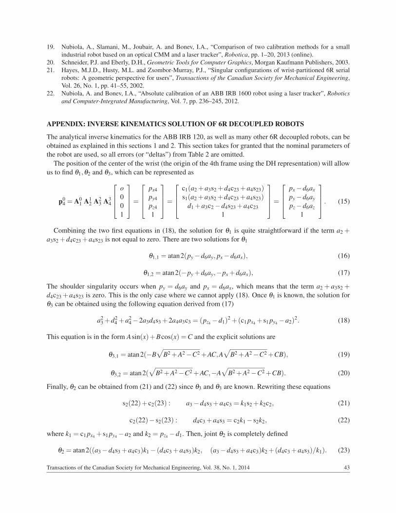
APPENDIX: INVERSE KINEMATICS SOLUTION OF 6R DECOUPLED ROBOTS

The analytical inverse kinematics for the ABB IRB 120, as well as many other 6R decoupled robots, can beobtained as explained in this sections 1 and 2. This section takes for granted that the nominal parameters ofthe robot are used, so all errors (or “deltas”) from Table 2 are omitted.

The position of the center of the wrist (the origin of the 4th frame using the DH representation) will allowus to find θ1,θ2 and θ3, which can be represented as

p04 = A0

1 A12 A2

3 A34

o001

=

px4py4pz41

=

c1(a2 +a3s2 +d4c23 +a4s23)s1(a2 +a3s2 +d4c23 +a4s23)

d1 +a3c2 −d4s23 +a4c231

=

px −d6ax

py −d6ay

pz −d6az

1

. (15)

Combining the two first equations in (18), the solution for θ1 is quite straightforward if the term a2 +a3s2 +d4c23 +a4s23 is not equal to zero. There are two solutions for θ1

θ1,1 = atan2(py −d6ay, px −d6ax), (16)

θ1,2 = atan2(−py +d6ay,−px +d6ax), (17)

The shoulder singularity occurs when py = d6ay and px = d6ax, which means that the term a2 + a3s2 +d4c23 +a4s23 is zero. This is the only case where we cannot apply (18). Once θ1 is known, the solution forθ3 can be obtained using the following equation derived from (17)

a23 +d2

4 +a24 −2a3d4s3 +2a4a3c3 = (pz4 −d1)

2 +(c1 px4 + s1 py4 −a2)2. (18)

This equation is in the form Asin(x)+Bcos(x) =C and the explicit solutions are

θ3,1 = atan2(−B√

B2 +A2 −C2 +AC,A√

B2 +A2 −C2 +CB), (19)

θ3,2 = atan2(√

B2 +A2 −C2 +AC,−A√

B2 +A2 −C2 +CB). (20)

Finally, θ2 can be obtained from (21) and (22) since θ3 and θ3 are known. Rewriting these equations

s2(22)+ c2(23) : a3 −d4s3 +a4c3 = k1s2 + k2c2, (21)

c2(22)− s2(23) : d4c3 +a4s3 = c2k1 − s2k2, (22)

where k1 = c1 px4 + s1 py4 −a2 and k2 = pz4 −d1. Then, joint θ2 is completely defined

θ2 = atan2((a3 −d4s3 +a4c3)k1 − (d4c3 +a4s3)k2, (a3 −d4s3 +a4c3)k2 +(d4c3 +a4s3)/k1). (23)


To calculate θ4,θ5 and θ6 we must use the information contained in R36, where

R36 = (R0

1 R12 R2

3)−1 R0

6 = R34 R4

5 R56 =

r1,1 r1,2 r1,3r2,1 r2,2 r2,3r3,1 r3,2 r3,3

=

∗ ∗ −c4s5−s5c6 s5s6 c5∗ ∗ s4s5

. (24)

We omitted the expressions marked with ∗ as they are not of interest. Two solutions for θ5 can be directlyobtained:

θ5,1 = atan2(√

1− r22,3,r2,3), (25)

θ5,2 = atan2(−√

1− r22,3,r2,3). (26)

Once θ5 is known, θ4 and θ6 are completely defined if θ5 is not equal to 0

θ4 = atan2(

r3,3

s5,−r1,3

s5

), (27)

θ6 = atan2(

r2,2

s5,−r2,1

s5

)(28)

Otherwise, if θ5 = 0 we have a wrist singularity and the equations can be simplified by forcingθ4 = 0. If all joints are limited in the range [−180◦,180◦], there are eight possible solutions (seehttp://youtu.be/xjjAiAmV05I). If this range is extended there can be more solutions.


Geometric Approach to Solving the Inverse … · Ce qui est nécessaire c’est uniquement le...

Documents

Transcript of Geometric Approach to Solving the Inverse … · Ce qui est nécessaire c’est uniquement le...