SYMPLECTIC GEOMETRY

VICENTE MUNOZ

1. Introduction

1.1. Classical Mechanics. Let U ⊂ Rn be an open subset of the n-dimensional space,where a particle of mass m moves subject to a force F (x). By Newton’s equation, thetrajectory x(t) of the particle satisfies the differential equation

mx(t) = F (x(t)) .

Using coordinates (x, y) ∈ U ×Rn, where (x, y) = (x, x), we have the equivalent equations:

(1)x(t) = y(t),y(t) = 1

mF (x(t)) .

Note that the space U × Rn is the tangent bundle TU .

We say that the force is conservative if F = −∇V , for some function V (x) on U , calledthe potential function of the mechanical system. In this case, a particle x(t) has kineticenergy K = 1

2m |x(t)|2 and potential energy V = V (x(t)). The total energy is

E(x, y) = K + V =12m |y(t)|2 + V (x(t)) .

It is easy to see that E is constant along time, by computing

dE

dt= m〈y(t), y(t)〉+ 〈∇V, x〉 = 〈y, F 〉 − 〈F, y〉 = 0.

The metric v 7→ m|v|2 gives an isomorphism between the tangent and cotangent bundles,TU → T ∗U , v 7→ p = mv. We may consider the particle as a trajectory on T ∗U , (x(t), p(t)),satisfying the equations

x(t) = 1mp(t) ,

p(t) = F (x(t)) .

The function H = K + V = 12m |p|

2 + V (x) defined on the cotangent bundle, is known asthe Hamiltonian of the mechanical system. The equations of the movement get rewrittenas

xi(t) = ∂H∂pi,

pi(t) = − ∂H∂xi

.

Partially supported through Special Action grant from MICINN (Spain) PCI2006-A9-0586.

1

2 VICENTE MUNOZ

Therefore a particle follows the flow of the vector field

(2) XH =∑i

(∂H

∂pi

∂

∂xi− ∂H

∂xi

∂

∂pi

)on the cotangent bundle.

This vector field can be computed intrinsically: T ∗U has a canonical 1-form λ (calledthe Liouville form), given by λ(x,α) = π∗α, for (x, α) ∈ T ∗U (i.e. x ∈ U , α ∈ T ∗xU),π : T ∗U → U . Locally, in coordinates (x, p), it is λ =

∑pj dxj . The 2-form ω = −dλ on

T ∗U is well-defined and has local expression

ω =∑j

dxj(t) ∧ dpj(t) .

Then XH is the unique vector field satisfying ω(XH , ·) = dH.

If we want to develop mechanics intrinsically, we have to use a smooth manifold M inplace of U . We have used a metric at several points: to compute the gradient of V , for thekinetic energy, etc. However, the formulation with the hamiltonian does not use this extrainformation. If we have the hamiltonian H, then XH in (2) can be extracted in an intrinsicway. Just note that T ∗M comes equipped with a 1-form λ and a 2-form ω = −dλ, and XH

satisfies ω(XH , ·) = dH.

Now, even we may forget about T ∗M and take any 2n-dimensional manifold Q with a2-form like ω. This is enough for theoretical purposes. Such pair (Q,ω) is known as asymplectic manifold. Thus, geometric mechanics take place in a symplectic manifold. Ituses a function H whose symplectic flow (that is, the flow of XH) leaves ω invariant (thatis, LXH

ω = 0). So the particles follow a flow which is by symplectomorphisms.

Now our interest is to understand what type of manifolds can be symplectic.

1.2. Complex manifolds. A complex manifold M of dimension n is a Hausdorff topo-logical space endowed with an atlas A = (Uα, φα) consisting of charts φα : Uα →φα(Uα) ⊂ Cn, which are homeomorphisms onto open sets of Cn, and whose changes ofcharts φα φ−1

β : φβ(Uα ∩ Uβ) → φα(Uα ∩ Uβ) are biholomorphisms (holomorphic mapswhose inverses are also holomorphic).

The primary examples of complex manifolds are the smooth algebraic projective varieties:take the complex projective space CPN , with projective coordinates [z0 : . . . : zN ]. Letf1(z0, . . . , zN ), . . . , fr(z0, . . . , zN ) be a collection of homogeneous polynomials and considerthe zero set

Z(f1, . . . , fr) = [z0 : . . . : zN ] ∈ CPN | f1(z0, . . . , zN ) = · · · = fr(z0, . . . , zN ) = 0 ⊂ CPN .

This is a complex manifold of dimension N − r when it is smooth. Smoothness happens ifthe Jacobian ∂(f1,...,fr)

∂(z0,...,zN ) has (maximal) rank r at every non-zero (z0, . . . , zN ).

SYMPLECTIC GEOMETRY 3

There are other ways to construct complex manifolds: for instance, if M is a complexmanifold, and Γ is a group acting discretely and freely on M by biholomorphisms, then thequotient M/Γ is again a complex manifold. For instance, take M = C2−0, and the groupZ generated by ϕ : M → M , ϕ(z, w) = (2z, 2w). The quotient M/Z is a smooth manifoldwhich is known as the Hopf surface. It is compact and diffeomorphic to S1 × S3.

There is a way to understand a complex manifold from the point of view of differentialgeometry. Let M be a complex manifold of complex dimension n. Then M is a smoothmanifold of dimension 2n. At each point p ∈M , the tangent space TpM is a 2n-dimensionalreal vector space which is actually a complex vector space. From linear algebra, this isequivalent to having a complex structure Jp : TpM → TpM (a linear map satisfying J2

p =−Id). This gives a tensor J ∈ End (TM) such that J2 = −Id.

In general, a pair (M,J), where J ∈ End (TM), J2 = −Id, is called an almost complexmanifold. To recover a complex atlas from (M,J) (and hence, for M to be a complex man-ifold), it is necessary that J satisfies an extra condition, called the integrability condition.The Nijenhuis tensor is defined as

NJ(X,Y ) = [X,Y ] + J [JX, Y ] + J [X, JY ]− [JX, JY ] ,

for vector fields X,Y . The famous theorem of Newlander-Niremberg says that (M,J) is acomplex manifold if and only if NJ = 0.

One of the most prominent questions in complex geometry is the following: given asmooth manifold M , does there exist J such that (M,J) is a complex manifold?

(1) The existence of J giving an almost-complex structure is a topological question.(2) Assuming the existence of an almost-complex structure, to find an integrable one is

an analytical problem.

1.3. Kahler manifolds. Let M be a complex manifold. A hermitian metric h is a tensorh : TM × TM → C, which is complex-linear in the first variable, satisfies h(v, u) = h(u, v),and h(u, u) > 0 for all non-zero u. Any complex manifold admits hermitian structures.

It is worth to note that the hermitian metric and the complex structure give rise to othertwo interesting tensors on M :

• a Riemannian metric: g(u, v) = Reh(u, v). Note that g(Ju, Jv) = g(u, v).• a 2-form ω(u, v) = g(u, Jv). Equivalently, ω(u, v) = Imh(u, v). Note that ω is

maximally non-degenerate, that is, ω(u, v) = 0,∀v =⇒ u = 0. This is equivalentto ωn 6= 0.

Locally, in coordinates (z1, . . . , zn), if the metric is written as h =∑hi dzi · dzj , then the

fundamental 2-form is ω = i2

∑hi dzi ∧ dzj . The non-degeneracy is obtained from

ωn

n!= det(hi)

(i2

)ndz1 ∧ dz1 ∧ . . . ∧ dzn ∧ dzn = volg.

4 VICENTE MUNOZ

We say that a (1, 1)-form α is positive if α = i2

∑ai dzi ∧ dzj , where (ai) is a positive

definite hermitian matrix. Equivalently (and more intrinsically), if α(Ju, u) > 0, for allnon-zero u.

Note that with ω and J we can recover g by g(u, v) = ω(Ju, v) and h by h(u, v) =g(u, v) + iω(u, v).

The projective space CPn has a very natural hermitian metric, which is obtained asfollows. Fix a basis on Cn+1, and take a hermitian metric h0 on Tp0CPn for a base-pointp0 = [1 : 0 : . . . , 0]. Then consider the (unique) metric h on CPn which is U(n + 1)-invariant (obtained by moving h0 with the matrices in this group). This can be obtainedmore intrinsically as follows: as TpCPn = Hom (lp,Cn+1/lp) (where lp ⊂ Cn+1 is the linedefined by p), we can give it the metric induced by that of Cn+1, for any p ∈ CPn. Takeaffine coordinates, that is, consider the open set U = [z0 : z1 : . . . : zn] | z0 6= 0 ⊂ CPn.Then U ∼= Cn where the point [1 : z1 : . . . : zn] has coordinates z = (z1, . . . , zn). Then themetric is written as

h(z) =(1 + |z|2)

∑dzi · dzi −

∑i,j zjzidzi · dzj

(1 + |z|2)2.

So the fundamental 2-form is

ω =i2

(1 + |z|2)∑dzi ∧ dzi −

∑i,j zjzidzi ∧ dzj

(1 + |z|2)2.

It is easy to calculate that

ω =i2∂∂ log(1 + |z|2) .

So we have dω = 0.

To sum up, ω is a positive closed (1, 1)-form. This means that [ω] is a 2-cohomologyclass. Moreover, [ω]n ∈ H2n(CPn) is non-zero, since it is a multiple of the volume form. Inparticular, [ω] 6= 0.

Definition 1. A Kahler manifold (M,J, ω) is a complex manifold (M,J) together with aclosed positive (1, 1)-form ω.

For a Kahler manifold, J is parallel, i.e. ∇J = 0.

Note that if S ⊂ CPn is a smooth algebraic complex manifold, then S is Kahler. This iseasy to see: just take as hermitian metric hS the restriction of the Fubini-Study metric ofCPn to S. Then the fundamental 2-form is ωS = ω|S . Therefore, it is a positive (1, 1)-formand dωS = 0.

Moreover, [ωS ] ∈ H2(S,Z) (where we denote by H2(S,Z) the image of H2(S,Z) →H2(S,R), which is a lattice). Moreover, the converse is true:

Theorem 2 (Kodaira, see [We]). If (M,J, ω) is a compact Kahler manifold and [ω] ∈H2(M,Z), then there is a holomorphic embedding M → CPN , for some large N .

SYMPLECTIC GEOMETRY 5

1.4. Topological properties. Let (M,J, ω) be a compact Kahler manifold of complexdimension n. Then M satisfies very striking topological properties:

(1) There is a Hodge decomposition of the cohomology of M ,

Hk(M,C) =⊕p+q=k

Hp,q(M)

and Hp,q(M) = Hq,p(M). Therefore, the Hodge numbers hp,q = dimHp,q(M)satisfy that hq,p = hp,q. So for k odd, the Betti numbers

bk(M) =∑p+q=k

hp,q =(k−1)/2∑p=0

(hp,k−p + hk−p,p

)= 2

(k−1)/2∑p=0

hp,k−p

are even.The Hopf surface has b1 = 1, hence it is not Kahler.

(2) Hard-Lefschetz theorem. The map

[ω]k : Hn−k(M)→ Hn+k(M)

is an isomorphism for each k = 1, . . . , n. This implies in particular that the map[ω]i on Hn−k(M) is injective for 1 ≤ i ≤ k, and so that bi+2 ≥ bi for 0 ≤ i ≤ n− 2.

(3) Fundamental group. When M is not simply-connected, there are striking resultsrestricting the nature of the fundamental group of M . These type of results canbe found in the nice book [ABCKT]. For instance a free product like Z ∗ Z cannotbe the fundamental group of a compact Kahler manifold. A group that can be thefundamental group of a compact Kahler manifold is called a Kahler group.

(4) Complex surfaces. If n = dimCM = 2, then the classification of complex surfaces[BPV] gives you exactly the diffeomorphism types of 4-manifolds M admitting acomplex (or Kahler) structure. This is a very short list (except for the surfaces ofgeneral type which are not fully understood). For instance, a consequence of theclassification is the following result: if M is complex and has even Betti number b1,then it admits a Kahler structure (maybe changing the complex structure).

(5) If M ⊂ CPN is a smooth projective manifold, then there exist complex submanifoldsin any dimension. By Bertini’s theorem, we may intersect with a generic linearsubspace Hr of codimension r so that Z = M∩Hr is a smooth complex submanifoldof complex dimension n−r. Moreover, the Lefschetz theorem on hyperplane sectionssays that

H i(M)→ H i(Z)

is an isomorphism for i = 0, 1, . . . , n− r − 1, and an epimorphism for i = n− r.(6) Homotopy groups. Suppose M is compact Kahler and simply-connected. Then

there are extra properties on the rational homotopy groups Vk = πk(M)⊗Q of M .The most relevant property is that of formality. To explain it, we have to explainsome notions of rational homotopy theory. We dedicate the next section to this.

6 VICENTE MUNOZ

1.5. Rational homotopy of simply-connected manifolds. A differential graded algebra(dga, for short) (A, d) is a positively graded commutative algebra A over the rational (orreal) numbers, with a differential d such that d(a · b) = (da) · b+ (−1)deg(a)a · (db). We shallassume that A0 = Q, A1 = 0. A dga (A, d) is said to be minimal if:

(1) A is free as an algebra, that is, A is the free algebra∧V over a graded vector space

V = ⊕V i, and(2) there exists a collection of generators xτ such that dxτ is expressed in terms of

preceding xµ, µ < τ . This implies that dxτ does not have a linear part, i.e., it livesin∧V >0 ·

∧V >0 ⊂

∧V .

A minimal model of a dga (A, d) is a minimal dga (M, d) with a dga morphism ρ :(M, d)→ (A, d) which is a quasi-isomorphism (quism), that is, ρ∗ : H∗(M)→ H∗(A) is anisomorphism on cohomology.

In the category of dga’s, there is an equivalence relation ∼ generated by quisms (that is,∼ is the minimal equivalence relation such that if ρ : (A1, d1) → (A2, d2) is a quism, then(A1, d1) ∼ (A2, d2)). Then the minimal model of a dga (A, d) is the canonical representativeof the quism equivalence class of (A, d).

A minimal model of a simply-connected differentiable manifold M is a minimal model(∧V, d) of the de Rham complex (ΩM,d) of differential forms on M (to be precise here,

we have to work over the field of real numbers). By the work of Sullivan, this contains theinformation of the rational homotopy of M :

V k ∼= (πk(M)⊗ R)∗, for all k ≥ 2 .

Now we are ready to introduce the notion of formality. A minimal model (M, d) is formalif there is a quism ψ : (M, d) → (H∗(M), 0). A dga (A, d) is formal if its minimal modelis so, that is, if (A, d) ∼ (H∗(A), 0). And a simply-connected manifold M is formal if itsminimal model is formal.

Theorem 3 ([DGMS]). Let M be a simply-connected compact Kahler manifold. Then M

is formal.

The proof of this uses essentially the fact that the dga of differential forms (Ω(M), d) ofa Kahler manifold has a bigrading given by the (p, q)-forms, together with some analyticalproperties of the Laplacian.

1.6. Symplectic manifolds. (See [MS] for general results on symplectic geometry.)

A symplectic manifold (M,ω) consists of a smooth manifold together with a 2-formω ∈ Ω2(M) satisfying:

• dω = 0,• ω is non-degenerate at every point.

SYMPLECTIC GEOMETRY 7

The second condition implies that M is of even dimension 2n. Then volM = 1n!ω

n

defines a volume form (in particular, M is naturally oriented). Note that ω works as anantisymmetric metric, as it gives an isomorphism TM → T ∗M , X 7→ iXω = ω(X, ·).

Let (M,ω) be a symplectic manifold of dimension 2n. A symplectic submanifold N ⊂Mis a submanifold such that ω|N is non-degenerate (hence a symplectic form on N). ALagrangian submanifold L ⊂ M is a submanifold of dimension n such that ω|L = 0 (n isthe maximum possible dimension for such situation to occur).

A symplectomorphism f : (M1, ω1) → (M2, ω2) is a smooth map such that f∗ω2 = ω1.For surfaces dimM = 2, a symplectic form on M is an area form, and a symplectomorphismis an area preserving map.

Note that a small perturbation of a symplectic ω, that is, a closed 2-form ω′ such that|ω − ω′|C1 < ε (for some small ε > 0), is still symplectic. If the cohomology class does notchange, we have the following result.

Lemma 4 (Moser’s stability). If ωt, t ∈ [0, 1] is a family of symplectic forms on M withω0 = ω, and [ωt] = [ω], then there exists a family ψt : (M,ω) → (M,ωt) of sympletomor-phisms. (Moreover, if ωt = ω over some subset A, then ψt = Id over A.)

Proof. As [ωt] = cte, d[ωt]dt = 0. So there are 1-forms αt such that dωt

dt = dαt. Using thenon-degeneracy of the symplectic forms, there are vector fields Xt such that iXtωt = −αt.Take the flow ψt produced by Xt. Let us check that ψ∗t ωt = ω, that is, that ψ∗t ωt = cte.We compute

d

dt(ψ∗t ωt) = ψ∗tLXtωt + ψ∗t

dωtdt

= ψ∗t (diXtωt + iXtdωt) + ψ∗t (dαt)

= ψ∗t (−dαt) + ψ∗t (dαt) = 0 ,

as required.

Locally, a symplectic manifold (M,ω) has a standard form, which is given by the well-known Darboux theorem.

Theorem 5 (Darboux). Let p ∈ M . Then there is a chart around p, (x1, y1, . . . , xn, yn),on which ω is written ω = dx1 ∧ dy1 + . . .+ dxn ∧ dyn.

Proof. To get Darboux theorem, we apply Moser’s stability lemma in a ball B centered at0 to the given 2-form ω and to the family ωt = f∗t ω, where ft : B → B, ft(x) = (1 − t)x,t ∈ [0, 1]. Note that for t = 1, ω1 is a constant symplectic form over B, as ω1(x) = ω(0),∀x ∈ B. In a suitable basis, it can be written ω(0) =

∑ni=1 dxi ∧ dyi (this is the canonical

form for a constant coefficient symplectic form).

8 VICENTE MUNOZ

This result says that there are no local invariants for a symplectic form. Therefore thereare only global invariants.

Let B ⊂M be a Darboux ball. This means that ω = dx1∧dy1 + . . .+dxn∧dyn. We canuse complex coordinates for the ball B, given as zj = xj + i yj , j = 1, . . . , n. In this way,we understand that B ⊂ Cn and the symplectic form gets rewritten as

ω =i2

(dz1 ∧ dz1 + . . .+ dzn ∧ dzn).

In particular, we see that we can arrange an almost complex structure J in the ball suchthat (B, J, ω) is a standard ball of Cn.

2. Hard methods: Analysis

In this section we are going to describe results which extend properties known in theKahler setting to the symplectic world. These methods usually require techniques of PDEson manifolds.

Let (M,ω) be a compact symplectic manifold. We say that an almost-complex structureJ on M is compatible with ω if g(u, v) = ω(Ju, v) defines a metric on M .

The relevant topological result is that there exists ω-compatible J ’s and that the spaceJω = J | J is ω-compatible is contractible. This means that the choice of J is in somesense unique.

This is proved as follows: ω produces a reduction of the structure group of TM fromGL(2n,R) to Sp(2n,R). But U(n) ⊂ Sp(2n,R) is the maximal compact subgroup. There-fore there are reductions to U(n) and they are given by the sections of the associatedbundle with fiber Sp(2n,R)/U(n), which is contractible. Note that giving a reduction ofthe structure group to U(n) is equivalent to giving an ω-compatible J . Finally, note thatU(n) = Sp(2n,R) ∩ SO(2n), so we have a reduction to SO(2n), i.e. a metric.

Now we have an almost-Kahler manifold (M,J, ω). This means that (M,J) is an almost-complex manifold with a symplectic form ω compatible with J .

2.1. Gromov-Witten invariants. Let (M,ω) be a symplectic manifold and J ∈ Jω. Fixa compact Riemann surface Σ of some genus g ≥ 0. This has a complex structure whichwe denote by j. A map u : Σ → M is pseudo-holomorphic if du : TΣ → TM is complexlinear. This means that du j = J du. We can write du ∈ Ω1(Σ, u∗TM), where u∗TM isa complex bundle. Decompose du into (1, 0) and (0, 1) components, du = ∂Ju+ ∂Ju, where

∂Ju =12

(du− J du j) , ∂Ju =12

(du+ J du j) .

Let A ∈ H2(M,Z) be a 2-homology class. The moduli space of pseudo-holomorphiccurves in the class A is

MgA = u : Σ→M |u∗[Σ] = A, du j = J du = u ∈ Map(Σ,M) |u∗[Σ] = A, ∂Ju = 0 .

SYMPLECTIC GEOMETRY 9

This has a nice structure:

• ∂Ju = 0 is an elliptic PDE on Map(Σ,M). ∂J is a section of the vector bundleE → M = Map(Σ,M), Eu = Ω0,1(u∗TM), u ∈ M. Note that M is of infinitedimension, and E is of infinite rank. The ellipticity amounts to say that the differenceof these two infinities, the dimension of M = Z(∂J) ⊂M, is finite.• After a suitable perturbation, ∂J is transverse to zero. SoM is a smooth manifold.• One has to quotient out by the automorphisms of u (which creates singularities).

To avoid this, one takes pointed curves (Σ, x1, . . . , xr). So the automorphism groupis just the identity. This gives rise to moduli spaces Mg,r

A .• If j is allowed to vary, we have moduli spaces Mg,r

A parametrizing (u, j, x1, . . . , xr).• The theory of Gromov allows to compactify Mg,r

A by adding trees of curves withbubbles and different reducible components. This gives rise to a compact spaceMg,r

A . The boundary is of high codimension is good cases.

There are well-defined evaluation maps

evxi :Mg,rA −→ M

u 7→ u(xi) .

Fix genus g = 0 and r = 3, so we deal with Σ = CP1 with three marked points, say0, 1,∞ ∈ CP1. We define the Gromov-Witten invariants of (M,ω) as

GWA(α, β, γ) = 〈ev∗0α ∪ ev∗1β ∪ ev∗∞γ, [M0,3A ]〉 , for α, β, γ ∈ H∗(M) .

Fix a basis αi of H∗(M). Then define the operation ∗ on H∗(M) by nA,ijk =GWA(αi, αj , αk), and

〈αi ∗ αj , αk〉 =∑A,k

nA,ijk qA ,

where we have to enlarge the coefficients to add extra variables qA, for each A ∈ H2(M,Z).

In good situations, the boundary Mg,rA −M

g,rA has high codimension. For instance, this

happens if M is positive, i.e. if c1(M) = λω, λ > 0. In such cases, we have the following:

Theorem 6 ([RT]). The operation ∗ is a ring structure on H∗(M), called the quantummultiplication. The quantum cohomology QH∗(M) = (H∗(M), ∗) is an invariant of thesymplectomorphism type of (M,ω).

This ring serves to distinguish symplectic structures. In this way, one can constructsymplectic 6-manifolds which are diffeomorphic, but not symplectomorphic nor deformationsymplectically equivalent.

By work of Taubes, a version of the Gromov-Witten invariants for 4-manifolds is equiv-alent to the Seiberg-Witten invariants (which are invariants of the diffeomorphism type ofa 4-manifold, constructed using gauge-theoretic techniques). This has allowed to construct

10 VICENTE MUNOZ

two homeomorphic 4-manifolds M1, M2, such that M1 is Kahler and M2 is symplectic butnon-Kahler: M2 is taken as a symplectic fiber connected sum (see Section 3.3) of a suitableKahler surface M1 along a symplectically knotted surface Σ ⊂ M1. Then M2 has Seiberg-Witten invariants different from those of all Kahler surfaces (here it is used the Kodairaclassification of complex surfaces).

2.2. Asymptotically holomorphic theory. Let (M,ω) be a symplectic 2n-manifold suchthat [ω] ∈ H2(M,Z) and fix an ω-compatible almost-complex structure J .

By the integrality of [ω], there is a complex line bundle L → M whose first Chern classis c1(L) = [ω]. This allows to construct a connection A on L whose curvature is FA = i

2πω.By construction, this connection has positive curvature.

We expand the metric by considering gk = kg for integers k ≥ 1. gk is associated toωk = kω, which is the curvature of the connection kA on L⊗k. Donaldson [Do1] developedthe asymptotically holomorphic theory in the search for substitutes of holomorphic sectionsof L⊗k. Let sk ∈ Γ(L⊗k), then ∂sk ∈ Ω0,1(L⊗k). If J is not integrable, then we cannotexpect to get holomorphic sections sk, but we may try to find sequences of sections (sk)such that |∂sk| → 0. More concretely, we call a sequence of sections (sk) asymptoticallyholomorphic (A.H.) if |∂sk|Cr ≤ Ck−1/2.

It is not very difficult to construct plenty of such sections. Actually, there are A.H.sections concentrated around any given point p ∈M (these play the role of approximationsof the Dirac delta). Here is where the positivity of the curvature plays a fundamental role.

Let B be a Darboux ball around p with coordinates (z1, . . . , zn), and ω = i2(dz1 ∧ dz1 +

. . .+ dzn ∧ dzn). We can take A = d+ π2

∑(zjdzj − zjdzj). So the section s = e−πk|z|

2/2 isholomorphic with respect to the standard (integrable) complex structure J0 on B and theconnection kA. From |NJ |g ≤ C, we have |NJ |gk

≤ Ck−1/2, so |∂Js| ≤ Ck−1/2. As s hasGaussian decay, it can be multiplied by a suitable bump function so that it can be extendedto the whole of M and still satisfies |∂Jsk| ≤ Ck−1/2.

The next step in Donaldson’s programme is to construct a section sk such that its zero-set gives a smooth (symplectic) submanifold Wk = Z(sk). Typically, for this one needstransversality of the section to the zero section, that is:

(3) ∇sk : TpM → L⊗kp

is surjective for each p ∈Wk. In this case, Wk is smooth and TpWk = ker(∇psk) at p ∈Wk.

As we have only approximate holomorphicity, we need to require a stronger statement (orexpressed in a different way, some amount of transversality). We say that sk is η-transverseif (3) does multiply the norm of vectors at least by η > 0. Therefore, as

∇sk = ∂sk + ∂sk ,

when ∂sk is very small (for k large), ∂sk is the main contribution, and it is non-zero.Moreover, ∂sk : TpM → L⊗kp

∼= C is complex linear, its zero set is a complex subspace and

SYMPLECTIC GEOMETRY 11

ker(∇sk) is very close to ker(∂sk). Therefore Wk = Z(sk) is smooth and close to beingcomplex. More accurately,

∠(TpWk, J(TpWk)) ≤ Ck−1/2 .

In particular, Wk is a symplectic submanifold, and PD[Wk] = c1(L⊗k).

Donaldson constructs η-transverse sections in a very clever way: first, he proves that ina ball Bgk

(x, r0), r0 > 0 fixed, one can perturb an A.H. sequence of sections by addingconcentrated sections around x, in such a way to obtain σ-transversality on the ball, byperturbing an amount δ, with σ and δ related by

σ = δ(log δ−1)−p

(p is a large integer, but fixed and independent of δ and k).

Then the process has to be iterated, but there is one complication. Due to the expansionof the metric, gk = kg, the balls Bgk

(x, 1) = Bg(x, k−1/2) get smaller, so we need C kn

balls to cover M . At each step we get transversality of lower amount, and after goingover all the balls, we get some transversality εk, with εk → 0, as k → ∞. To avoid this,the balls are sorted out in finitely many groups. In each group the balls are separated bya large gk-distance D > 0, and all the perturbations in the same group can be realizedsimultaneously, since the Gaussian decay implies that the perturbation in one ball does notreduce significatively the amount of transversality in the rest. Thus the number of timesthe perturbation process is carried out is independent of k. This reduces the amount oftransversality but keeps it over some ε > 0, independently of k.

Let us see another application of A.H. theory, which appears in [MPS]. This is theextension of the Kodaira embedding theorem to the symplectic setting. Let (M,ω) be asymplectic manifold with [ω] ∈ H2(M,Z), and J ∈ Jω. We look for A.H. sequences ofsections

s0k, . . . , s

Nk ∈ Γ(L⊗k) ,

(N is large, say N ≥ 2n+ 1) such that:

• sk = (s0k, . . . , s

Nk ) is a section of CN+1 ⊗ L⊗k which is η-transverse to zero. As

n = dimCM < N + 1, we cannot have that ∇sk is surjective, so it must be |sk| > η

over all of M . Thus there is a well-defined map

ψk : M → CPN , ψk(x) = [s0k : . . . : sNk ] .

• The complex linear map ∂ψk : TM → TCPN is η-transverse. This means that ∂ψkmultiplies the length of vectors at least by η. In particular, ψk is an immersion, andMk = ψk(M) ⊂ CPN satisfies that it is close to being complex.• ψk is injective (this is a generic position argument).

In particular, ψk : M → CPN are symplectic embeddings (after an extra small deforma-tion).

12 VICENTE MUNOZ

2.3. Lefschetz pencils. Let (M,ω) be a symplectic 2n-manifold such that [ω] ∈ H2(M,Z)is an integral class. Fix an ω-compatible almost-complex structure J . Donaldson [Do2]constructs a symplectic Lefschetz fibration for M which extends the Lefschetz fibrations foralgebraic projective varieties. Using A.H. theory, he looks for A.H. sequences of sections

s0k, s

1k ∈ Γ(L⊗k)

which satisfy the following transversality properties:

• (s0k, s

1k) is an η-transverse sequence of sections. In particular, the zero set Bk =

Z(s0k, s

1k) is a symplectic submanifold of codimension 4. There is a well-defined map

φk = [s0k, s

1k] : M −Bk → CP1 .

• s0k is η-transverse to zero, so that the fiber of φk over ∞ is smooth, and removing

it we have a map φk(x) = s1ks0k

: M − F∞ → C. Note that the fibers Fλ = φ−1k (λ),

λ ∈ C, can be compactified to Fλ = Fλ ∪Bk, which is smooth along Bk. These arecodimension 2 symplectic submanifolds (off the singular locus of φk).• The singular locus of φk (where φk is not submersive) consists of finitely many points

∆k ⊂ M − Bk. At each p ∈ ∆k, a transversality requirement for the holomorphicHessian ∂∂φk of φk allows to achieve (after an extra perturbation) a local model asfollows: there are Darboux coordinates (z1, . . . , zn) ∈ B ⊂ Cn around p such that

φk = λ+ z21 + . . .+ z2

n.

This gives a double point singularity at p for the fiber Fλ, λ = φk(p).

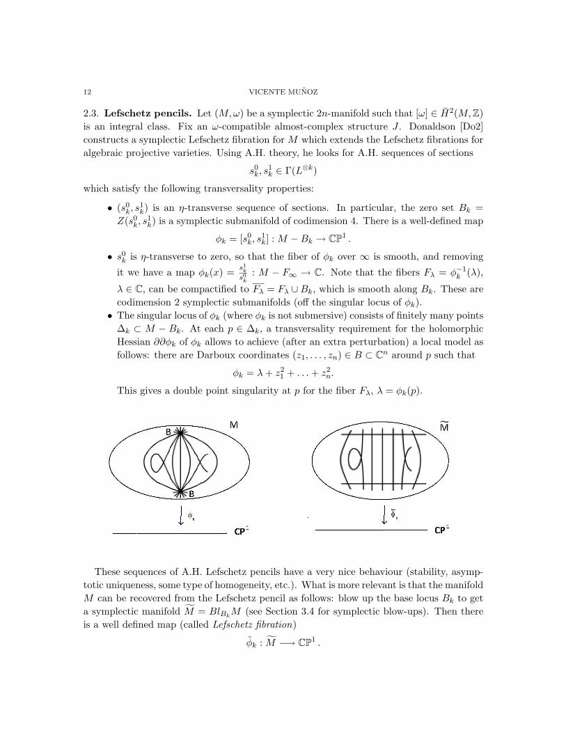
These sequences of A.H. Lefschetz pencils have a very nice behaviour (stability, asymp-totic uniqueness, some type of homogeneity, etc.). What is more relevant is that the manifoldM can be recovered from the Lefschetz pencil as follows: blow up the base locus Bk to geta symplectic manifold M = BlBk

M (see Section 3.4 for symplectic blow-ups). Then thereis a well defined map (called Lefschetz fibration)

φk : M −→ CP1 .

SYMPLECTIC GEOMETRY 13

Consider a base point ∗ ∈ CP1 whose corresponding fiber F is smooth. We have atrue fibration with fiber F (symplectic of dimension 2n − 2) over CP1 − Crit(φk), whereCrit(φk) = φk(∆k) are the critical values (we assume that the images in CP1 of the criticalpoints are different; this is easily achieved with a small perturbation). When we approach acritical value λ→ λ0 ∈ Crit(φk), the fiber Fλ0 is obtained by contracting some Lagrangiansphere Sn−1 ⊂ Fλ = F (called the vanishing cycle). Moreover, the monodromy of a smallloop around λ0 is a symplectomorphism of F called a Dehn twist around Sn−1 (it consistsof cutting along Sn−1 and regluing it with a twist).

This allows to recover M out of some algebraic information extracted from the Lefschetzpencil. Theoretically this would allow to classify symplectic structures (at least on lowdimension, 2n = 4). In practice the problem gets intractable since we have to allow k 0for A.H. Lefschetz pencils.

3. Soft methods: Topology

The topological methods address the following question:

Can we construct symplectic manifolds and detect that they do not admit Kahler metrics?

One of the ways to achieve this is to see that there are very few topological restrictions fora symplectic manifold to exist, whereas there are very strong restrictions on the topologicalproperties of Kahler manifolds. This produces symplectic manifolds M such that there isno Kahler manifold M ′ which is homotopy equivalent to M .

We would like to remind here that in the case of 4-manifolds there are also gauge-theoreticresults which allow to produce pairs of manifolds M1, M2 which are homeomorphic but notdiffeomorphic, M1 being Kahler, M2 being symplectic but without Kahler structure.

3.1. Nilmanifolds. A nilpotent group is a simply-connected Lie group G satisfying thefollowing nilpotency condition: if we define the nested sequence of subgroups Gi by G1 = G,Gi = [Gi−1, G] for i ≥ 2, then there is some N > 0 such that GN = 0. Any nilpotent groupof dimension n is diffeomorphic to Rn, as a differentiable manifold.

A nilmanifold is a compact n-dimensional manifold of the form M = G/Γ, where Γ is adiscrete (cocompact) subgroup of a nilpotent group G. The Lie algebra g of G is a nilpotentLie algebra: if we define the nested sequence of Lie subalgebras gi by g1 = g, gi = [gi−1, g]for i ≥ 2, then there is some N > 0 such that gN = 0 (note that gi is the Lie algebra of Gi).

The right invariant forms of M , Ω∗inv(M) ⊂ Ω∗(M), are in bijective correspondence withthe forms at the neutral element of G, that is, Ω∗inv(M) ∼=

∧∗(g∗). By a theorem of Nomizu[No], the inclusion (Ω∗inv(M), d) → (Ω∗(M), d) is a quism. Therefore, (M, d) = (

∧∗(g∗), d)is the minimal model of M . Write g = 〈e1, . . . , en〉 and g∗ = 〈x1, . . . , xn〉. Then if [ei, ej ] =

14 VICENTE MUNOZ∑k>i,j a

kijek, we have that

(∧∗

(x1, . . . , xn), d), dxk = −∑i,j<k

akij xi ∧ xj ,

is the minimal model of M .

A symplectic form can be obtained by a 2-form ω =∑aij xi ∧ xj satisfying dω = 0 and

ωn/2 = c x1 ∧ x2 ∧ · · · ∧ xn, c 6= 0. Note that the volume form is vol = x1 ∧ · · · ∧ xn.

A nilmanifold M can’t be formal unless it is a torus. If there is a quism

ψ : (∧∗

(g∗), d) −→ H∗(∧∗

(g∗), d) ,

then arrange x1, . . . , xn in increasing order so that the closed elements are x1, . . . , xr, andψ(xr+1) = . . . = ψ(xn) = 0. This would imply that ψ(vol) = 0 (which is impossible), unlessr = n. This means that M is a torus.

The Kodaira–Thurston manifold . Let H be the Heisenberg group, that is, the connectednilpotent Lie group of dimension 3 consisting of matrices of the form

a =

1 x z

0 1 y

0 0 1

,

where x, y, z ∈ R. Let Γ be the discrete subgroup of H consisting of matrices whose entriesare integer numbers. So the quotient space M = Γ\G is compact.

A basis of right invariant vector fields is ∂∂z ,∂∂y + x ∂

∂z ,∂∂x. Therefore the generators of

g∗ are α = dx, β = dy, γ = dz − x dy. Note that

dγ = −dx ∧ dy = −α ∧ β .

The Kodaira–Thurston manifold KT is the product KT = M × S1. Then, there are1–forms α, β, γ, η on KT such that dα = dβ = dη = 0, dγ = −α ∧ β. Note that

ω = α ∧ γ + β ∧ η

defines a symplectic form since dω = 0 and ω2 = 2α ∧ γ ∧ β ∧ η 6= 0.

KT is therefore a non-formal symplectic 4-manifold, hence it cannot admit a Kahlerstructure. This was the first example of a symplectic manifold not admitting a Kahlerstructure, as shown by Thurston [Th]. But he showed this by checking that b1 = 3 (thiscomes from Nomizu’s theorem, which gives H1(KT ) = 〈[α], [β], [η]〉). KT was also a mani-fold introduced by Kodaira as a manifold admitting a complex structure but not a Kahlerone.

Massey products. There is an easier way to prove the non-formality of a manifold, whichavoids the use (and computation) of minimal models.

SYMPLECTIC GEOMETRY 15

Let M be a smooth manifold and let ai ∈ Hpi(M), 1 ≤ i ≤ 3, be three cohomologyclasses such that a1 ∪ a2 = 0 and a2 ∪ a3 = 0. Take forms αi on M with ai = [αi] and writeα1 ∧ α2 = dξ, α2 ∧ α3 = dη. The Massey product of the classes ai is defined as

〈a1, a2, a3〉 = [α1 ∧ η + (−1)p1+1ξ ∧ α3] ∈ Hp1+p2+p3−1(M)a1 ∪Hp2+p3−1(M) +Hp1+p2−1(M) ∪ a3

.

(The denominator in the quotient group is due to the indeterminacy in the choice of ξ andη.)

The relevant result is that if M has a non-trivial Massey product then M is non-formal.This is due to the following: Massey products can easily be defined on any dga, and thenthey can be seen to be transferred through quisms. Therefore if M is formal, one cantransfer the Massey product through (Ω∗(M), d) ∼ (H∗(M), 0). But in the latter dga, allMassey products are zero, as the differential is zero.

Finally, to prove this way that KT is non-formal, it is enough to compute the Masseyproduct:

〈[α], [α], [β]〉 = [0 · β + α ∧ (−γ)] = −[α ∧ γ] 6= 0 in H2(KT ) .

Another example. In a similar way, we can also obtain a symplectic nilmanifold X ofdimension 4 which is non-formal but which does not admit any complex structure. SuchX has minimal model (

∧∗(g∗), d), with g∗ = 〈α, β, γ, η〉, dγ = α ∧ β, dη = α ∧ γ. The2-form ω = α ∧ η + β ∧ γ is symplectic. The first Betti number of X is even, b1 = 2, asH1(X) = 〈[α], [β]〉. This implies that if X admits a complex structure then it also has aKahler structure, by a result of Kodaira (or by the classification of complex surfaces [BPV]).But this is not possible, since X is non-formal as it is a nilmanifold which is not a torus.So X cannot admit a complex structure at all.

3.2. Symplectic fibrations. One can construct symplectic structures on fibrations in somesituations in which both the fiber and the base have symplectic structures.

Suppose that (F, σ) is a symplectic manifold. A symplectic fibration over B with fiber(F, σ) consists of a fibration F → M

π−→ B such that there is a cover Uα of B forwhich there are trivializations ψα : π−1(Uα)

∼=→ F × Uα, and the changes of trivializationsψα ψ−1

β : F × (Uα ∩ Uβ) → F × (Uα ∩ Uβ) are of the form (f, x) 7→ (ϕx(f), x), whereϕx : (F, σ)→ (F, σ) is a symplectomorphism.

It is not automatic that there is a global closed 2-form on M restricting to σ at each fiberFx = π−1(x). At least we need a cohomological condition: that there exists a ∈ H2(M)with a|Fx = [σ]. This justifies condition (1) in the theorem below.

Theorem 7 (Thurston). Let (F, σ)→M → B be a symplectic fibration, and assume that:

(1) there exists a ∈ H2(M) with a|Fx = [σ],(2) (B,ωB) is a symplectic manifold.

16 VICENTE MUNOZ

Then there is a symplectic structure on M .

Proof. First, fix a representative η of a. We want to find another representative restricting toa symplectic form on each fiber. Consider a covering B =

⋃Uα such that π−1(Uα) ∼= F×Uα.

Let σα be the 2-form on π−1(Uα) defined as the pull-back of σ from F . Then σα = η+dψα,ψα ∈ Ω1(F ×Uα). Take a partition of unity ρα on B subordinated to Uα, and considerthe closed 2-form

σ = η +∑

d(ραψα) .

For b ∈ B, σ|Fb= η|Fb

+∑ρα(b)dψα|Fb

=∑ρα(b)(η + dψα)|Fb

=∑ρα(b)σα|Fb

. Butσα|Fb

= σ for any b ∈ Uα. This implies that σ|Fb= σ, for all b ∈ B.

Finally, consider ω = π∗ωB + ε σ, for small ε > 0. It is easy to see that this is symplecticon M .

This can be used in many situations. For instance, it can be used to prove that KT is asymplectic manifold. Note that KT has (local) coordinates (x, y, z, w), where (x, y, z) arethe coordinates for the Heisenberg group and w is the coordinate for the extra S1 factor.The action of Γ is as follows:

(x, y, z, w) 7→ (x+ 1, y, z + y, w),

(x, y, z, w) 7→ (x, y + 1, z, w),

(x, y, z, w) 7→ (x, y, z + 1, w),

(x, y, z, w) 7→ (x, y, z, w + 1).

The projection (x, y, z, w) 7→ (x,w) gives a mapKT → T 2 and the fiber is T 2. Note that thisis a symplectic fibration, since there is no monodromy when going around the w-directionand the monodromy around the x-direction is the symplectic map (y, z) 7→ (y, z + y).

Using Theorem 7, with a = [dy ∧ dz], we have a symplectic structure on KT .

3.3. Fiber connected sum. Let (M1, ω1), (M2, ω2) be two symplectic manifolds and sup-pose that (N,ω) is a symplectic manifold of dimension 2n− 2, with two symplectic embed-dings:

ıj : (N,ω) −→ (Mj , ωj) , j = 1, 2.

Let νj → N be the normal bundle to ıj . Then if ν1∼= ν∗2 are isomorphic bundles (where ν∗2

is the dual bundle to ν2), we can glue M1 and M2 along N with the following constructionof Gompf [Go].

Consider a neighborhood Uj ⊂Mj of Nj = ıj(N), which can be identified with the ε-discbundle in νj . So there is a fibration D2

ε → Uj → Nj , j = 1, 2. Now remove the closed δ-discbundle Vj ⊂ Uj in νj , with δ < ε, to get a fibration by annuli Aε,δ = z ∈ C | δ < |z| < ε,

Aε,δ → Uj − Vj → N .

SYMPLECTIC GEOMETRY 17

Since a symplectic form for Aε,δ is just an area form, and a symplectic map is an area-preserving map, there is an orientation-reversing self-symplectomorphism

f : Aε,δ → Aε,δ ,

sending the inner boundary onto the outer one and viceversa. This can be done paramet-rically to produce a diffeomorphism F : U1 − V1 → U2 − V2. The fiber connected sum isdefined as

M = M1#NM2 := (M1 − V1) ∪F (M2 − V2) .

By Moser’s stability lemma, one can arrange that the symplectic forms of U1 − V1 andU2 − V2 coincide. In this way, M is endowed with a symplectic structure.

This was used by Gompf to produce many examples of symplectic non-Kahler manifolds.

Theorem 8. Let Γ be any finitely presented group, and let 2n ≥ 4. Then there is asymplectic manifold M of dimension 2n with fundamental group π1(M) ∼= Γ.

Proof. Let us give the main ideas of the proof (for details, see [Go]). For simplicity, focuson the 4-dimensional case. Take a presentation of the group Γ = 〈x1, . . . , xr|r1, . . . , rs〉 withgenerators and relations. Consider a 4-manifold M whose fundamental group contains afree group of r-elements, e.g. a surface of genus r times a two-torus, M = Σr×T 2. ThereforeΓ is a quotient of π1(M). Then construct tori Tj inside M which are Lagrangian and forwhich the image of π1(Tj)→ π1(M) generate exactly the kernel of π1(M) Γ. These areeasily arranged to be disjoint: a loop in Σr times a loop in the T 2 factor suffice.

Now note that if Tj ⊂ M is a Lagrangian 2-torus, then the normal bundle to Tj istrivial (an ω-compatible almost-complex J produces an isomorphism between the tangentand normal bundles to Tj). This allows to perturb the symplectic form on D2 × Tj tomake Tj symplectic. Once that Tj is symplectic, we do a fiber connected sum of M andsome other manifold X along Tj . The chosen symplectic 4-manifold X should containa symplectic 2-torus T ⊂ X such that X − T is simply connected (there are plenty ofexamples with these properties, using e.g. Kahler surfaces). In this way, the resulting 4-manifold M ′ = M#Tj=TX has π1(M ′) = π1(M)/π1(Tj). Repeating the construction overall Tj we eventually get a 4-manifold whose fundamental group is Γ.

As a consequence, if Γ is a non-Kahler group, then any compact symplectic manifold(M,ω) with π1(M) ∼= Γ cannot be Kahler.

3.4. Symplectic blow-up. Let (M,ω) be a symplectic manifold. Fix a point p ∈M . Wecan define the blow-up at p as follows: consider a Darboux chart B around p, with complexcoordinates (z1, . . . , zn) such that ω = i

2(dz1 ∧ dz1 + . . . dzn ∧ dzn). Consider the blow-upof B at the origin. This is the manifold

B = ((z1, . . . , zn), [w1, . . . , wn]) ∈ B × CPn−1|(z1, . . . , zn) = λ(w1, . . . , wn), λ ∈ C.

18 VICENTE MUNOZ

Note that there is a projection π : B → B. The preimage of any q 6= 0 is a point (q, [q]).The preimage of 0 is E = π−1(0) = 0 × CPn−1 ∼= CPn−1 ⊂ B. This is a codimension 2submanifold.

Now let us give B a symplectic form. For B ×CPn−1 we take the symplectic form givenas β = ω+ εΩ, where ω is the symplectic form on B, Ω is the Fubini-Study form on CPn−1,and ε > 0. This is actually a Kahler form for B ×CPn−1. As B ⊂ B ×CPn−1 is a complexsubmanifold, β is a Kahler form (hence symplectic) over B.

Finally, define the blow-up M by gluing M − p with B along the difeomorphism B −p

π∼= B − E. To give a symplectic structure to M , we have to glue the symplectic formsas follows. Consider Ω and note that when restricted to B−p, it is exact, hence Ω = dψ.Take a bump function of B which is one in a neigbourhood of E, and zero off B, andconsider d(ρψ). This can be extended as zero off B and as Ω near E. Now consider

ωM

= ω + ε d(ρψ).

Near E, this equals the form β = ω + εΩ, which is symplectic. Off B, it coincides with ω,also symplectic. And in the intermediate region, it is a small perturbation of ω, which isstill symplectic (for ε > 0 small).

The blow-up construction can be extended to blow-up a symplectic manifold along anembedded symplectic submanifold, as proved by McDuff [Mc].

Theorem 9. Let (M,ω) be a symplectic manifold, and let N ⊂M be a symplectic subman-ifold of codimension 2r ≥ 4. Then there is a well-defined symplectic blow-up of M alongN , which is a symplectic manifold (M = BlNM, ω), together with a map π : M →M suchthat:

• E = π−1(N) → N is the fibration which is the (complex) projectivization of thenormal bundle of N in M .• π : M − E → M − N is a diffeomorphism. Moreover, ω and π∗ω coincide off a

neighbourhood of E.

Proof. To prove this, we have to introduce an ω-compatible almost-complex structure J asfollows: first take some J on TN . Then on the symplectic normal bundle νN → N , definedas νN (p) = (TpN)o = u ∈ TpM |ω(u, TpN) = 0, p ∈ N , we put a complex structure J , sothat νN becomes a complex vector bundle. Then this J can be extended to a neighborhoodof N and later to the whole of M .

Now we consider a neighborhood U ⊂ M of N which is symplectomorphic to the discbundle νε ⊂ νN , whose fibers are ε-balls Dε ⊂ νN (p). We may blow-up νε → N along thezero section, by doing a fiberwise blow-up. The result is a fiber bundle

Dε → BlN νε → N .

SYMPLECTIC GEOMETRY 19

This has a map π : BlN νε → νε. Finally, we glue BlN νε andM−N along BlN νε−π−1(N) ∼=U−N . The symplectic forms would be glued in a similar fashion as for the case of blowing-upat a point.

The symplectic blow-up was used to produce the first examples of compact symplecticmanifolds which are simply-connected and non-Kahler.

Take a symplectic embedding of the Kodaira-Thurston manifold into a projective space,KT ⊂ CPn. Note that it should be n ≥ 5. Consider the symplectic blow-up

M = BlKTCPn .

It is simply-connected since CPn is so, but it cannot be Kahler because it is non-formal.This is seen easily with a Massey product. Note that the exceptional divisor E ⊂ M is acodimension 2 submanifold and there is a fibration CPn−3 → E

π→ KT . The dual formassociated to E, ν ∈ Ω2(M), is a closed 2-form compactly supported in a neighborhood ofE. Note that this gives sense to expressions like π∗a ∧ ν, for any form a ∈ Ω(KT ). Thefollowing Massey product

〈[π∗α ∧ ν], [π∗α ∧ ν], [π∗β ∧ ν]〉 = −[π∗(α ∧ γ) ∧ ν3]

is non-zero (we need n − 2 ≥ 3 for this non-vanishing). Therefore M is not formal. Thisproduces simply-connected symplectic non-formal manifolds on any dimension 2n ≥ 10.

3.5. Symplectic resolution of singularities. An orbifold (of dimension n) is a topologi-cal space M with an atlas with charts modeled on U/Gp, where U is an open set of Rn andGp is a finite group acting linearly on U with only one fixed point p ∈ U . An orbifold M

contains a discrete set ∆ of points p ∈M for which Gp 6= Id. The complement M −∆ hasthe structure of a smooth manifold. The points of ∆ are called singular points of M . Forany singular point p ∈ ∆, a small neighbourhood of p is of the form B/Gp, where B is aball in Rn.

An orbifold form α ∈ Ω∗orb(M) consists ofGp-equivariant forms on U , for each chart U/Gp,with the obvious compatibility condition. A symplectic orbifold (M,ω) is a 2n-dimensionalorbifold M together with a 2-form ω ∈ Ω2

orb(M) such that dω = 0 and ωn 6= 0 at everypoint.

Definition 10. A symplectic resolution of a symplectic orbifold (M,ω) is a smooth sym-plectic manifold (M, ω) and a map π : M →M such that:

(a) π is a diffeomorphism M − E → M − ∆, where ∆ ⊂ M is the singular set andE = π−1(∆) is the exceptional set.

(b) The exceptional set E is a union of (possibly intersecting) smooth symplectic sub-manifolds of M of codimension at least 2.

(c) ω and π∗ω agree on the complement of a small neighbourhood of E.

The following result is in [FM].

20 VICENTE MUNOZ

Theorem 11. Any symplectic orbifold has a symplectic resolution.

Proof. Consider a ball B/Gp around a singular point p ∈ ∆. Take Darboux coordinates onB, and a complex structure on B. So B/Gp is an (open) complex singular variety. We takea resolution of singularities in the complex setting (say, using Hironaka desingularisationprocess, which ensures that a suitable sequence of blow-ups yield eventually a smoothcomplex variety), B/Gp → B/Gp. This complex variety has a Kahler form. Finally we glue

M − p to B/Gp along B/Gp − p, and glue the symplectic forms as in the case of theblow-up of a symplectic manifold at a point.

This result was used in [FM] to produce the first example of a simply-connected sym-plectic non-formal manifold of dimension 8. This goes as follows.

Consider the complex Heisenberg group HC, that is, the complex nilpotent Lie group ofcomplex matrices of the form

a =

1 u2 u3

0 1 u1

0 0 1

,

and let G = HC × C, where C is the additive group of complex numbers. We denoteby u4 the coordinate function corresponding to this extra factor. In terms of the natural(complex) coordinate functions (u1, u2, u3, u4) on G, we have that the complex 1-formsµ = du1, ν = du2, θ = du3 − u2 du1, η = du4 are right invariant and

dµ = dν = dη = 0, dθ = µ ∧ ν.

Let Λ ⊂ C be the lattice generated by 1 and ζ = e2πi/3, and consider the discretesubgroup Γ ⊂ G formed by the matrices in which u1, u2, u3, u4 ∈ Λ. We define the compact(parallelizable) nilmanifold

M = Γ\G.We can describe M as a principal torus bundle

T 2 = C/Λ →M → T 6 = (C/Λ)3,

by the projection (u1, u2, u3, u4) 7→ (u1, u2, u4).

Now introduce the following action of the finite group Z3

ρ : G → G

(u1, u2, u3, u4) 7→ (ζ u1, ζ u2, ζ2 u3, ζ u4).

The complex 2-formω = i µ ∧ µ+ ν ∧ θ + ν ∧ θ + i η ∧ η

is actually a real form, it is closed and satisfies ω4 6= 0. Hence ω is a symplectic form onM . Moreover, ω is Z3-invariant. Hence the space

(M = M/Z3, ω)

SYMPLECTIC GEOMETRY 21

is a symplectic orbifold. By Theorem 11, this can be desingularized to a smooth symplecticmanifold M of dimension 8.

It remains to see that M is simply connected and non-formal. This follows from thesame assertions for the orbifold M . It is not difficult to see that M is simply connected, butwe shall content ourselves to see here that b1(M) = 0. By Nomizu’s theorem, H1(M) =〈Re(µ), Im(µ),Re(ν), Im(ν),Re(η), Im(η)〉 ∼= C⊕C⊕C, and the action of Z3 is by rotations.So

H1(M) = H1(M)Z3 = 0 .

The non-formality of M is more difficult to check. Clearly M is non-formal since it isa nilmanifold which is not a torus. To quotient by Z3 kills ‘part of’ the minimal model(for instance, it kills the cohomology of degree 1, where one usually writes down Masseyproducts). One has to check that enough non-formality remains after the Z3-quotient isperformed. Details can be found in [FM].

References

[ABCKT] J. Amoros, M. Burger, K. Corlette, D. Kotschick, D. Toledo, Fundamental groups of compact

Kahler manifolds, Math. Sur. and Monogr. 44, Amer. Math. Soc., 1996.

[BPV] W. Barth, C. Peters and A. Van de Ven, Compact complex surfaces, Springer-Verlag, 1984.

[DGMS] P. Deligne, P. Griffiths, J. Morgan, D. Sullivan, Real homotopy theory of Kahler manifolds, Invent.

Math. 29 (1975), 245–274.

[Do1] S. K. Donaldson. Symplectic submanifolds and almost-complex geometry. J. Diff. Geom., 44, 666-705

(1996).

[Do2] S. K. Donaldson. Lefschetz pencils on symplectic manifolds. J. Diff. Geom. 53, 205–236 (1999).

[FM] M. Fernandez, V. Munoz An 8-dimensional non-formal simply connected symplectic manifold, Ann.

of Math. (2), 167 (2008), 1045–1054.

[Go] R. Gompf, A new construction of symplectic manifolds, Ann. of Math. (2) 142 (1995), 527–597.

[Mc] D. McDuff, Examples of symplectic simply connected manifolds with no Kahler structure, J. Diff.

Geom. 20 (1984), 267–277.

[MS] D McDuff, D Salamon, Introduction to symplectic topology, Oxford Mathematical Monographs, Oxford

University Press (1998).

[MPS] V. Munoz, F. Presas, I. Sols. Almost holomorphic embeddings in grassmanians with applications to

singular symplectic submanifolds. J. reine angew. Math. 547, 149–189 (2002).

[No] K. Nomizu, On the cohomology of compact homogeneous spaces of nilpotent Lie groups, Ann. of Math.

59 (1954), 531-538.

[RT] Y. Ruan and G. Tian, A mathematical theory of quantum cohomology, Jour. Diff. Geom. 42 1995,

259-367.

[Th] W.P. Thurston, Some simple examples of symplectic manifolds, Proc. Amer. Math. Soc. 55 (1976),

467–468.

[We] R.O. Wells, Differential Analysis on Complex Manifolds, Graduate Texts in Math. 65, Springer-Verlag,

1980.

Instituto de Ciencias Matematicas CSIC-UAM-UCM-UC3M, Consejo Superior de Investiga-

ciones Cientıficas, Serrano 113 bis, 28006 Madrid, Spain

22 VICENTE MUNOZ

Facultad de Matematicas, Universidad Complutense de Madrid, Plaza Ciencias 3, 28040

Madrid, Spain

E-mail address: vicente.munoz@imaff.cfmac.csic.es