Geomatica II Training Guide...Geomatica II Geomatica II Page 8 PCI Geomatics Figure 1. GDB in...
168
Transcript of Geomatica II Training Guide...Geomatica II Geomatica II Page 8 PCI Geomatics Figure 1. GDB in...


Geomatica II
Course guide
Geomatica Version 2018

Page iv PCI Geomatics
©2018 PCI Geomatics Enterprises, Inc.® All rights reserved.
COPYRIGHT NOTICE
Software copyrighted © by PCI Geomatics Enterprises, Inc.,
90 Allstate Parkway, Suite 501
Markham, Ontario L3R 6H3, CANADA Telephone number: (905) 764-0614
The Licensed Software contains material that is protected by international Copyright Law and trade secret law, and by international treaty provisions, as well as by the laws of the country in which this software is used. All rights not granted to Licensee herein are reserved to Licensor. Licensee may not remove any proprietary notice of Licensor from any copy of the Licensed Software.

PCI Geomatics Page 5
Contents
Geomatica II 6
Introduction 6 About this training guide 6 Geospatial data structures 7 GDB technology in Geomatica 7 PCIDSK and Geomatica 8 PCIDSK file format 8 Working with Geomatica Focus 9
Module 1: Image classification 15
Lesson 1.1 - Unsupervised classification 17 Lesson 1.2 - Aggregating classes 21 Lesson 1.3 - Initializing supervised classification 26 Lesson 1.4 - Collecting training sites 31 Lesson 1.5 - Analyzing training sites 36 Lesson 1.6 - Running a supervised classification 42 Lesson 1.7 - Assessing classification accuracy 44 Lesson 1.8 - Post-classification filtering and vectorization 48
Module 2: DEM Editing in Focus 55
Lesson 2.1 Quality Assessment Tools 55 Lesson 2.2 Editing roads, Bridges or Overpasses 60
Module 3: Spatial analysis in Focus 67
Lesson 3.1 - Buffering vectors 67 Lesson 3.2 - Dissolving vectors 72 Lesson 3.3 - Finding area neighbors 79 Lesson 3.4 - Performing a spatial overlay 85 Lesson 3.5 - Performing a statistical overlay 90 Lesson 3.6 - Performing a suitability overlay 93
Module 4: Publishing map projects 98
Lesson 4.1 - Introduction to a map project 99 Lesson 4.2 - Building a map structure 106 Lesson 4.3 - Representing vector data 112 Lesson 4.4 - Building a map surround 120
Module 5: Working with Modeler 124
Lesson 5.1 - Building a model to convert raster to vector 125 Lesson 5.2 - Subsetting in Modeler 138 Lesson 5.3 - Batch processing in Modeler 145
Optional Modules 153
Module 1: Performing atmospheric correction 153
Lesson 1.1 – Cloud Masking & Haze Removal 156 Lesson 1.2 - Atmospherically correcting imagery to Ground Reflectance 160

Geomatica II Geomatica II
Page 6 PCI Geomatics
Geomatica II
Introduction
Welcome to Geomatica II, an intermediate level course focusing on image
classification, atmospheric correction, spatial analysis, map compilation, and batch
processing in Modeler. This guide is written for new and experienced users of
geospatial software.
This manual contains five modules. Each module contains lessons that are built on
basic tasks that you are likely to perform in your daily work. They provide
instruction for using the software to carry out essential processes while sampling
key Geomatica applications and features.
Please note that training for OrthoEngine is not included in this guide. If you require
more information about OrthoEngine training, please go to the PCI Geomatics
Training Department website at the link below:
http://www.pcigeomatics.com/resources/geomatica/training
About this training guide
The scope of this guide is confined to the core PCI software applications included in
the Geomatica suite; however, some remote sensing concepts are reviewed in the
modules and lessons.
The following modules are included in this course:
Module 1: Image classification
Module 2: Performing atmospheric correction
Module 3: Spatial analysis in Focus
Module 4: Publishing map projects
Module 5: Working with Geomatica Modeler
Each module in this book contains a series of hands-on lessons that let you work
with the software and a set of sample data. Lessons have brief introductions
followed by tasks and procedures in numbered steps.
The data you will use in this course can be found in the GEO II Data folder provided
in the accompanying data installation file. You should install these data to your hard
disk.
Students who are unfamiliar with the file structure of geospatial data should
carefully review the remaining sections in this introduction before moving on to the
course work in the modules.
Geomatica II Geomatica II
PCI Geomatics Page 7
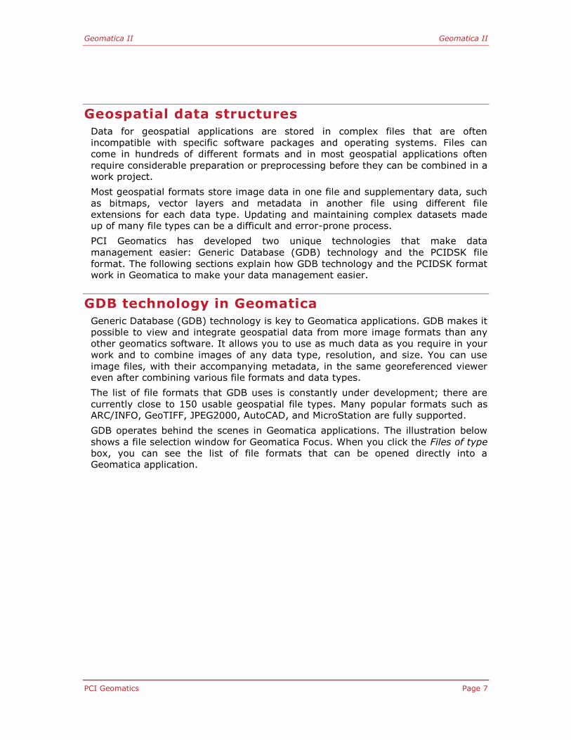
Geospatial data structures
Data for geospatial applications are stored in complex files that are often
incompatible with specific software packages and operating systems. Files can
come in hundreds of different formats and in most geospatial applications often
require considerable preparation or preprocessing before they can be combined in a work project.
Most geospatial formats store image data in one file and supplementary data, such
as bitmaps, vector layers and metadata in another file using different file
extensions for each data type. Updating and maintaining complex datasets made up of many file types can be a difficult and error-prone process.
PCI Geomatics has developed two unique technologies that make data
management easier: Generic Database (GDB) technology and the PCIDSK file
format. The following sections explain how GDB technology and the PCIDSK format work in Geomatica to make your data management easier.
GDB technology in Geomatica
Generic Database (GDB) technology is key to Geomatica applications. GDB makes it
possible to view and integrate geospatial data from more image formats than any
other geomatics software. It allows you to use as much data as you require in your
work and to combine images of any data type, resolution, and size. You can use
image files, with their accompanying metadata, in the same georeferenced viewer even after combining various file formats and data types.
The list of file formats that GDB uses is constantly under development; there are
currently close to 150 usable geospatial file types. Many popular formats such as ARC/INFO, GeoTIFF, JPEG2000, AutoCAD, and MicroStation are fully supported.
GDB operates behind the scenes in Geomatica applications. The illustration below
shows a file selection window for Geomatica Focus. When you click the Files of type
box, you can see the list of file formats that can be opened directly into a Geomatica application.

Geomatica II Geomatica II
Page 8 PCI Geomatics
Figure 1. GDB in Geomatica
With GDB technology, you can work through a mapping project by assembling
raster and vector data from different sources and different file formats without the
need to preprocess or reformat the data. Together, GDB and Geomatica read, view, and process distribution formats, and read, edit, and write exchange formats.
PCIDSK and Geomatica
PCIDSK files contain all of the features of a conventional database and more. They
store a variety of data types in a compound file that uses a single file name
extension. The image data are stored as channels and auxiliary data are stored as
segments. All data types are stored together in the file using .pix as the file name
extension. The data type and format of the component determines whether
searching, sorting and recombining operations can be performed with the software application tools.
In PCIDSK files, images and associated data, called segments, are stored in a
single file. This makes it easier to keep track of imagery and auxiliary information.
PCIDSK file format
Using a single file for each set of data simplifies basic computing operations. Since
all data is part of the same file you can add or remove parts of it without having to
locate, open, and rename more files.
PCIDSK files are identical in all operating environments and can be used on
networked systems without the need to reformat the data.

Geomatica II Geomatica II
PCI Geomatics Page 9
PCIDSK files Conventional files
Figure 2. Conventional files and PCIDSK files
Working with Geomatica Focus
Geomatica Focus is designed to work with dozens of data formats, through GeoGateway, and to take advantage of the PCIDSK file format.
When you start Geomatica on your system desktop, the Geomatica Toolbar opens
and the Focus application starts automatically. The Geomatica toolbar includes a
button for each of the major Geomatica applications: Focus, OrthoEngine, Modeler, EASI, Chip Manager, FLY!, SPTA, Mosaic Tool and Historical Air Photo (HAP) Tool.
Figure 3. Geomatica Toolbar
When you pass your mouse over a button on the toolbar the name of the
application appears as a ToolTip beside your mouse pointer.
Figure 4 shows the basic parts of the Focus window.
Image Fi les
Training site files
Histogram fi les
Image channels
Training site segments
Histogram segments
Saved Separately using differentSaved as a single file using the fi le namefile name extensionsextension .pix

Geomatica II Geomatica II
Page 10 PCI Geomatics
A. Menu bar B. Toolbar C. Maps and Files tabs D. Maps and Files tree list E. View Area F. Status bar
Figure 4. Focus window
Managing data in Focus
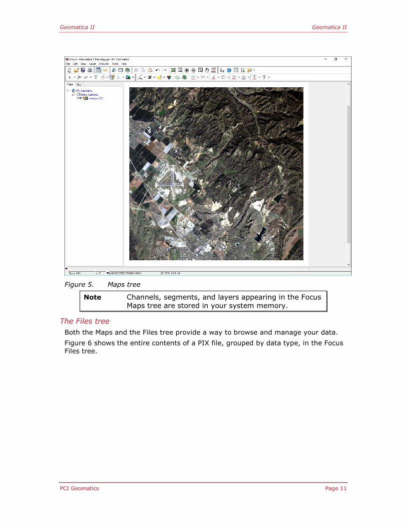
In Figure 5, you can see what Focus looks like with an open PCIDSK file. On the
right, in the Focus view area, you can see the file imagery. On the left you can see
both image and auxiliary data as channels and segments in the Maps and Files
trees. The color channels are separated into red, green, and blue layers and show the electromagnetic spectrum (EMS) frequency range for the source image.
The Maps tree
The Maps tree lists the areas, layers, channels, and segments that make up the
image in the view area. The Maps tree components are stored in your system memory.
It contains layers that can be shown in the Focus view area, including the channels
that make up the layers and any results from algorithms that are stored in system
memory. Items appearing in the Maps tree are not necessarily data saved on a hard disk and they do not affect the original data files.
Geomatica II Geomatica II
PCI Geomatics Page 11
Figure 5. Maps tree
Note Channels, segments, and layers appearing in the Focus
Maps tree are stored in your system memory.
The Files tree
Both the Maps and the Files tree provide a way to browse and manage your data.
Figure 6 shows the entire contents of a PIX file, grouped by data type, in the Focus
Files tree.
Geomatica II Geomatica II
Page 12 PCI Geomatics
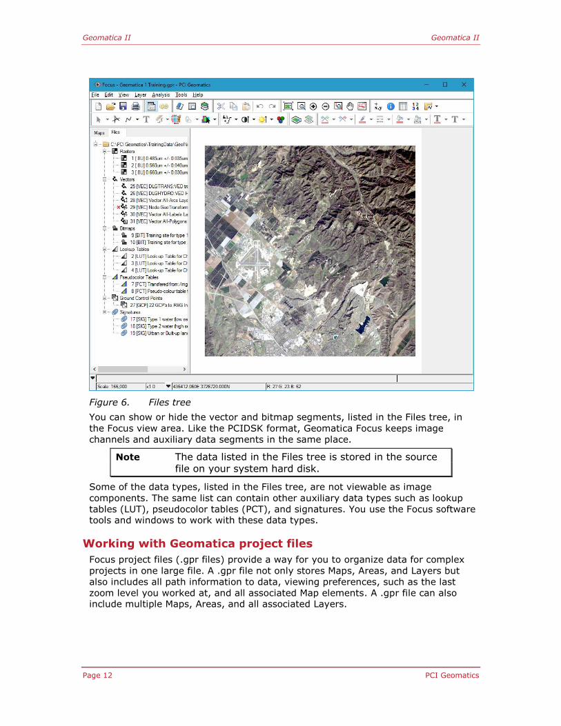
Figure 6. Files tree
You can show or hide the vector and bitmap segments, listed in the Files tree, in
the Focus view area. Like the PCIDSK format, Geomatica Focus keeps image
channels and auxiliary data segments in the same place.
Note The data listed in the Files tree is stored in the source
file on your system hard disk.
Some of the data types, listed in the Files tree, are not viewable as image
components. The same list can contain other auxiliary data types such as lookup
tables (LUT), pseudocolor tables (PCT), and signatures. You use the Focus software tools and windows to work with these data types.
Working with Geomatica project files
Focus project files (.gpr files) provide a way for you to organize data for complex
projects in one large file. A .gpr file not only stores Maps, Areas, and Layers but
also includes all path information to data, viewing preferences, such as the last
zoom level you worked at, and all associated Map elements. A .gpr file can also include multiple Maps, Areas, and all associated Layers.

Geomatica II Geomatica II
PCI Geomatics Page 13
Understanding Maps, Areas, Layers, and Segments
The files, listed in the Maps tree, are a hierarchy of elements that make up a
Geomatica project. Maps tree elements have common properties that you can
control from the Maps and Files trees, the menu bar, and context-sensitive shortcuts.
Maps
The element at the top of the hierarchy is the Map. This is the workspace that holds
all of the data for your work. You can have more than one map in a project. The
Map is also a page that contains the extents of your project canvas. You can adjust
the map size to control the size of your printed output. When Focus is in Map View
mode, you can adjust the size and position of the image relative to the canvas. You
can also add surround elements to your map.
Areas
The Area element holds the file boundaries for either image or vector layers. Areas
can include multiple layers and segments for a geographical region and you can
have as many areas in a project as you wish. Each Area has a unique
georeferencing system. When new image files are added to an area they are referenced automatically.
Layers
Layers hold the data that are displayed in the view area. Made up of segments,
layers can be rearranged in the Maps tree to vary the image in the view area. You
change the order of layers by dragging them up or down the Maps tree. When you move a layer, you move the segments that belong to it as well.
Segments
Segments are all of the components that make up a layer. For example, channels,
vectors, bitmaps, and lookup tables (LUT) can all be considered as segments when they appear as part of a layer.
Starting your work
In the lessons that follow, you will have an opportunity to carry out several tasks
using Focus. Your overall goal is to become familiar with the software and to see
how you can use Geomatica in your own work.


PCI Geomatics Page 15
Module 1: Image classification
About this Module
Module 1 has eight lessons:
Lesson 1.1 - Unsupervised classification
Lesson 1.2 - Aggregating classes
Lesson 1.3 - Initializing supervised classification
Lesson 1.4 - Collecting training sites
Lesson 1.5 - Analyzing training sites
Lesson 1.6 - Running a supervised classification
Lesson 1.7 - Assessing classification accuracy
Lesson 1.8 - Post-classification filtering and vectorization
The classification process
Digital image classification, also known as spectral pattern recognition, uses the
spectral information for each pixel in an image file to group pixels into common
spectral themes. Classified images are thematic maps containing a mosaic of pixels
belonging to different classes.
The objective of the classification process is to assign all pixels in an image to a
finite number of categories, or classes of data, based on their pixel values. If a
pixel satisfies a certain set of criteria, then it is assigned to the class that
corresponds to that criteria.
Classification distinguishes between information classes and spectral classes.
Information classes are ground cover categories you are interested in identifying
from the original spectral data in your imagery. They could include: agricultural
crop types, plant or forest species, or geological material types. Spectral classes
are groups of pixels with similar brightness values or spectral characteristics.
In comparing information classes with spectral classes, you must determine how
the classified image data is to be used and how the spectral classes translate into
information classes. There are two different image classification methods:
unsupervised and supervised.

Module 1: Image classification Geomatica II
Page 16 PCI Geomatics
Unsupervised classification
This is a highly computer-automated procedure. It allows you to specify parameters
that the computer uses as guidelines to uncover statistical patterns in the data. In
an unsupervised classification the software automatically divides the range of
spectral values contained in an image file, into classes. With Focus you can choose
the number of classes the data is divided into. The classified results report the
proportions of spectral values in the image and can therefore indicate the
prevalence of specific ground covers.
A classification report can indicate the presence of a specific ground cover because
a proportion of the classified pixels fall within its known spectral signature. In such
a case, you need to know what the spectral signature of the target ground cover is
in order to identify its presence.
Supervised classification
Supervised classification is more closely controlled by you than unsupervised
classification. In this process, you select recognizable regions within an image, with
help from other sources, to create sample areas called training sites. Your training
sites are then used to train the computer system to identify pixels with similar
characteristics.
Knowledge of the data, the classes desired, and the algorithm to be used, is
required before you begin selecting your training sites. Carrying out effective
supervised classification may take practice. It requires you to develop the ability to
recognize your target features and visual patterns in your image data. If the
classification is accurate, each resulting class will correspond to the training areas
that you originally identified.
Supervised training requires you to construct your information classes from a priori
knowledge of the data, such as:
What types of classes need to be extracted? You may be looking for soil types, land use areas, or specific types of vegetation.
What classes are most likely to be present in the data? In the case of
classifications intending to identify land cover types, you’ll need to have some idea of the actual types of soil or types of vegetation represented by the data.
Once training areas have been collected, Focus will use one of several algorithms to
determine how to classify the unknown pixels in the dataset based on the numerical
signatures for each training class.
In this module, you will use the Focus classification tools to carry out both
supervised and unsupervised classifications. Additionally, accuracy assessment and
post-classification filtering and vectorization will be performed.

Geomatica II Module 1: Image classification
PCI Geomatics Page 17
Lesson 1.1 - Unsupervised classification
In this lesson you will:
Start a new classification session
Initialize an unsupervised classification
Run a classification and review the report
Unsupervised classification
An unsupervised classification organizes image information into discrete classes of
spectrally similar pixel values. To perform unsupervised classification with Focus,
you use windows to configure your input files and to choose the number of classes
that will be differentiated.
When you have finished configuring your classification, you run the process. Focus
automatically classifies the spectral values in the image data. You can view the
classification results in the Focus view area and as a classification report.
Starting a new classification session
To begin working on this module, make sure Focus is open on your desktop. You
will initialize your classification session from the Focus window.
You will perform your unsupervised classification on the golden_horseshoe.pix file.
Before you initialize your classification session you will need to open the
golden_horseshoe.pix file From the GEOII Data folder.
To open golden_horseshoe.pix
1. On the Project toolbar, click Open File.
A File Selector window opens.
2. From the GEOII Data folder, open golden_horseshoe.pix.
To initialize a classification session
1. In the Maps tree, right-click the golden_horseshoe.pix layer.
2. In the Image Classification submenu, click Unsupervised.
The Session Selection window opens.
Figure 7. Session Selection window
3. Click New Session.
The Session Selection window closes and the Session Configuration
window opens.

Module 1: Image classification Geomatica II
Page 18 PCI Geomatics
Figure 8. Session Configuration window
4. In the Description box, type Unsupervised Session.
5. Set the Red, Green, and Blue color values to channels 3, 2 and 1
respectively, or to your preferred RGB color combination.
6. In the Input Channels column, select channels 1 through 6.
7. In the Output Channel column, select channel 7.
This channel will store your classification results.
8. Click OK.
The Session Configuration window closes and the Unsupervised
Classification window opens.
Focus also adds a Classification MetaLayer to the Maps tree to help you manage
your classification session.
Unsupervised classification
The Unsupervised Classification window allows you to choose the algorithm and the
parameters you want to use for your classification.
To run the unsupervised classification
1. In the Unsupervised Classification window, select the K-means algorithm.
2. Under K-Means Parameters, for the Max Class, enter 30.
3. For Max Iteration, enter 30.
4. Click OK.
Focus runs the classification using the K-means algorithm. A Progress
Monitor opens showing the progress of the classification. When the
classification is complete, the Progress Monitor closes. A Classification
Report opens and the classified image displays in the Focus view area.

Geomatica II Module 1: Image classification
PCI Geomatics Page 19
Figure 9. The classified image
The Maps tree now shows the Classification MetaLayer for the unsupervised
classification above the original image layers. The Classification MetaLayer manages
the classification session and also stores configuration information about your
session. It lists the Output layer and the three-band reference image. You can view
the original image by turning off the visibility of the Output layer within the
Classification MetaLayer.
Reading the classification report
The classification report indicates the distribution of pixel values across the number
of classes that you chose in the Classify window. The report includes a date stamp
and the file path for your classified imagery. The classification algorithm is listed
with the input channels and the channel where your results are stored.
Below the identifying information, the report lists the number of clusters created by
the classification alongside the details for each cluster. Clusters are groups of pixels
with similar spectral properties.

Module 1: Image classification Geomatica II
Page 20 PCI Geomatics
Figure 10. Classification report
The Classification Report tells you how many pixels make up each class, as well as
the mean brightness value and the standard deviation for each of the six input
image channels.
Lesson summary
In this lesson you:
Started a new classification session
Initialized an unsupervised classification
Ran a classification and reviewed the report

Geomatica II Module 1: Image classification
PCI Geomatics Page 21
Lesson 1.2 - Aggregating classes
In this lesson you will:
Combine classes into new aggregate classes
Class aggregation
Unsupervised image classifiers do not always provide the desired number of truly
representative classes. Aggregation can be used to combine separate classes into
one class after a classification. A maximum of 255 classes can be reassigned in a
single session.
A common approach in unsupervised classification is to generate as many cluster
classes as possible. With the benefit of reference data or first-hand knowledge of
the scene, the analyst then aggregates the spectral clusters into meaningful
thematic classes.
To set up the reference image
1. Turn off the visibility of the Classification Metalayer.
The default false color composite of the Landsat-7 scene is visible in the
view area. You will now change this to a typical false color composite.
2. Click the + sign to the left of the golden_horseshoe.pix: 1,2,3 layer in the
Maps.
3. Right-click the red component and select band 4.
4. Right-click the green component and select band 3.
5. Right-click the blue component and select band 2.
6. Reapply the adaptive enhancement from the toolbar.
A 4,3,2 false color composite is displays in the view area. In this
composite, vegetation is red, bare soil and urban areas are blue or cyan
and water is black.
7. Turn on the visibility of the Classification Metalayer.
To set up for aggregating classes
1. In the Maps tree, right-click the Classification MetaLayer.
2. Select Post-classification Analysis and then click Aggregation.
The Channel Setup window opens.

Module 1: Image classification Geomatica II
Page 22 PCI Geomatics
Figure 11. Channel Setup window
3. For the Input channel, select channel 7.
This is the channel that will be aggregated. It is typically the result of an
unsupervised classification.
4. As the Output channel, select channel 8.
The results of the aggregation will be stored in this channel.
5. Click OK.
The Aggregate window opens.
Figure 12. Aggregate window
To aggregate classes
1. Under View Controls, select Current Classes.
This displays the classes currently selected in the Input Classes list.
Geomatica II Module 1: Image classification
PCI Geomatics Page 23
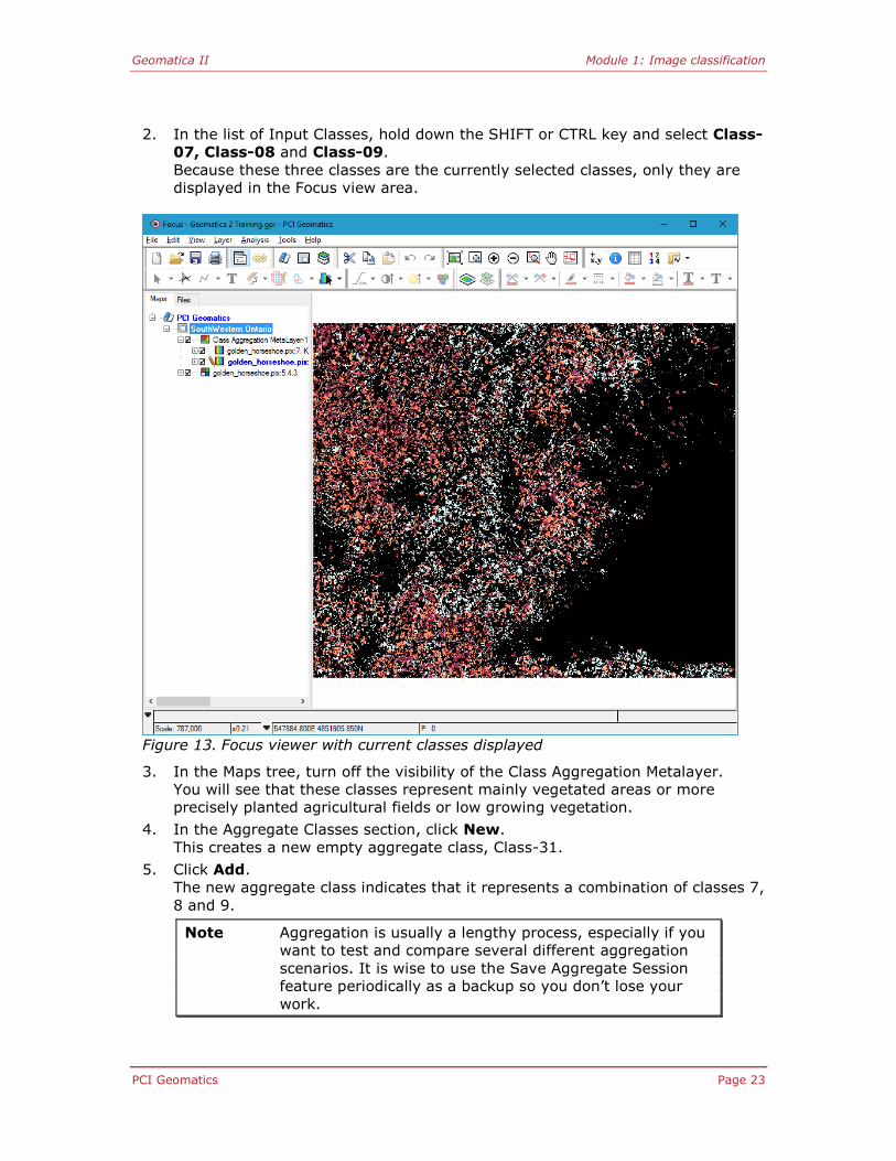
2. In the list of Input Classes, hold down the SHIFT or CTRL key and select Class-
07, Class-08 and Class-09.
Because these three classes are the currently selected classes, only they are
displayed in the Focus view area.
Figure 13. Focus viewer with current classes displayed
3. In the Maps tree, turn off the visibility of the Class Aggregation Metalayer.
You will see that these classes represent mainly vegetated areas or more
precisely planted agricultural fields or low growing vegetation.
4. In the Aggregate Classes section, click New.
This creates a new empty aggregate class, Class-31.
5. Click Add.
The new aggregate class indicates that it represents a combination of classes 7,
8 and 9.
Note Aggregation is usually a lengthy process, especially if you
want to test and compare several different aggregation
scenarios. It is wise to use the Save Aggregate Session
feature periodically as a backup so you don’t lose your
work.
Module 1: Image classification Geomatica II
Page 24 PCI Geomatics
During class aggregation, you need to compare the reference, or original image to
the classified image to determine which classes to aggregate. To complete this
process, you will be turning the Classification Metalayer off to see the reference
image below, and then turning it back on to see the results of the aggregation.
To complete the class aggregation
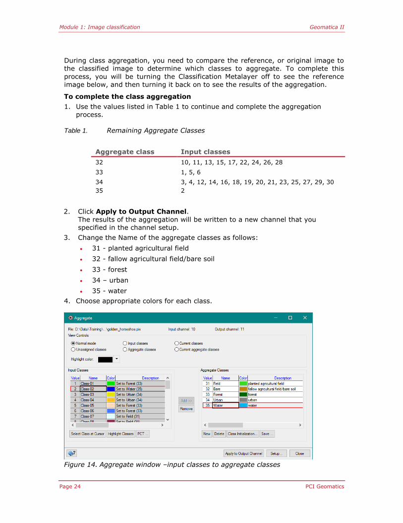
1. Use the values listed in Table 1 to continue and complete the aggregation
process.
Table 1. Remaining Aggregate Classes
Aggregate class Input classes
32 10, 11, 13, 15, 17, 22, 24, 26, 28
33 1, 5, 6
34
35
3, 4, 12, 14, 16, 18, 19, 20, 21, 23, 25, 27, 29, 30
2
2. Click Apply to Output Channel.
The results of the aggregation will be written to a new channel that you
specified in the channel setup.
3. Change the Name of the aggregate classes as follows:
31 - planted agricultural field
32 - fallow agricultural field/bare soil
33 - forest
34 – urban
35 - water
4. Choose appropriate colors for each class.
Figure 14. Aggregate window –input classes to aggregate classes

Geomatica II Module 1: Image classification
PCI Geomatics Page 25
5. Click Apply to Output Channel.
The name and color changes will be written to the output file.
To end the classification session
In the Maps tree, right-click the Class Aggregation MetaLayer and select
Remove. The metalayer is removed.
Lesson summary
In this lesson you:
Combined classes into new aggregate classes

Module 1: Image classification Geomatica II
Page 26 PCI Geomatics
Lesson 1.3 - Initializing supervised classification
In this lesson you will:
Open a new supervised classification session
Add image channels
Change the RGB reference image
Initialize a supervised classification
Supervised classification
In supervised classification, you must rely on your own pattern recognition skills
and a priori knowledge of the data to help Focus determine the statistical criteria
(signatures) for data classification. To select reliable training sites, you should have
some information, either spatial or spectral, about the pixels that you want to
classify.
The location of a specific characteristic, such as a land cover type, may be known
through ground truthing. Ground truthing refers to the acquisition of knowledge
about the study area from field work analysis, aerial photography, or personal
experience. Ground truth data is considered to be the most accurate (true) data
available about the area you want to study. They should be collected at the same
time as the remotely-sensed data, so that the data corresponds as much as
possible. Global positioning systems are useful tools to conduct ground truth
studies and collect training sites.
Initializing supervised classification
Like unsupervised classification, supervised classification is initialized as a session
in Focus. The initialization procedure also helps you manage subsequent
classifications on the same files, without having to re-initialize a new session each
time.
To initialize a classification session
1. In the Maps tree, right-click the golden_horseshoe.pix layer.
2. In the Image Classification submenu, click Supervised.
The Session Selection window opens.
Figure 15. Session Selection window
3. Click New Session.
The Session Configuration window opens.

Geomatica II Module 1: Image classification
PCI Geomatics Page 27
Figure 16. Session Configuration window
The Session Configuration window lists the image channels contented in the
golden_horseshoe.pix file. Focus automatically assigns RGB values to the first three
channels. You use the Session Configuration window to select the exact
combination of channels for your purpose. You can assign the color channels that
define the reference image for collecting your training sites and for doing any post-
classification analysis.
To configure the session
1. In the Description box, type Supervised Classification.
Note When naming classification sessions, enter a name in the
Description box that will distinguish your current
classification from others you create.
2. Beside the Description box, click Add Layer.
The Add Image Channels window opens.
3. Add 2 8-bit channels to golden_horseshoe.pix.
The first empty channel will contain training sites; the second will contain
the supervised classification result.
Figure 17. Adding Image Channels for Supervised Classification

Module 1: Image classification Geomatica II
Page 28 PCI Geomatics
4. Click Add.
The channels are added to the golden_horseshoe.pix file.
Specifying the reference image
Recall that supervised classification requires you to rely on your own pattern
recognition skills and a priori knowledge of the data to help Focus determine the
spectral signatures for classifying the data. To select reliable training sites, you
should know either spatial or spectral information about the pixels that you want to
classify.
You will need to visually identify your training areas from familiar colors in the
imagery. Therefore, you need to select a three-band combination that helps you
distinguish features of interest in your images. The session configuration window
automatically assigns the first three channels to the reference image displayed in
the Focus view area.
Next, you will select three bands to be displayed as a reference image in the Focus
view area.
To change the RGB channels
In the Session Configuration window, click the Red, Green, and Blue table
cells beside the corresponding spectral bands or TM bands you wish to
display.
Figure 18. Session Configuration window
After you have set the RGB values to display a three-band composite, you will
select which channels the classification will be based on. You will include all six
multispectral bands in the golden_horseshoe.pix file.
To select your input and output channels
1. In the Input Channels column, click channels 1 through 6.
Next, you will select a channel for collecting your training sites. You will use an
empty channel that you created at the start of this lesson.
2. In the Training Channel column, select channel 9.
3. In the Output Channel column, select channel 10.
This channel will store the classification results.

Geomatica II Module 1: Image classification
PCI Geomatics Page 29
Figure 19. Supervised Classification Session Configuration window
4. Click OK.
The Session Configuration window closes and the Training Site Editor window
opens. Focus also adds a Classification MetaLayer to the Maps tree to help you
manage your classification session. The metalayer contains three layers: the
training channel, the three-band composite you selected and the output layer.
Figure 20. Training Site Editor window
You have now initialized your classification session and are ready to begin collecting
and editing your training sites.
Lesson summary
In this lesson you:
Opened a new supervised classification session
Added image channels
Changed the RGB reference image
Initialized a supervised classification

Module 1: Image classification Geomatica II
Page 30 PCI Geomatics

Geomatica II Module 1: Image classification
PCI Geomatics Page 31
Lesson 1.4 - Collecting training sites
In this lesson you will:
Create training sites manually
Create training sites with raster seeding
Change the color of your training sites
Training sites and ground cover
Training sites are areas in an image that are representative of each of the land
cover classes that you want to define. Focus examines the pixel values within the
training sites in order to compile a statistical signature for each training site class.
The training signatures serve as the interpretation key for each pixel in the image.
All pixels in the image are compared to the signatures and then classified.
You designate training sites based on samples of different surface cover types in
your imagery by drawing colored regions or areas over the parts of the image that
are likely to be the information classes you want to extract.
You cannot know for certain what the actual ground cover in the image is by
referencing only the image; therefore, samples (training sites) must be based on
familiarity with the geographical region and knowledge of the actual surface cover
types in the image.
Next, you will use the Training Site Editor to create training sites for the following
broad categories: bare soil, planted fields, urban, water and forest.
To create a new class
1. In the Class menu on the Training Site Editing window, click New.
Class-01 appears in the editing table. The editing table automatically assigns a
numbered cell for your first class.
Figure 21. Training Site Editor with one class
2. In the Name column, type bare soil.

Module 1: Image classification Geomatica II
Page 32 PCI Geomatics
Next you will draw a training site for bare soil over the reference image in the Focus view area.
Collecting training sites
After naming bare soil in the Training Site Editor, you can use the Focus Editing
Toolbar commands to draw training sites for this class over the image in the Focus
view area.
To select a drawing tool
1. If necessary, in the Maps tree, below the Classification MetaLayer, select
the PCT layer labeled Training areas.
You can use either Line, Polygon, Rectangle, Ellipse, Trace or Raster
Seeding to create training sites. In this first example, you will use
Polygon.
2. On the Editing toolbar, click the New Shapes arrow.
3. Select Polygon.
Figure 22. New Polygon Shape tool
You are now ready to draw a training site over the Reference Image in the work
area. In this lesson, you will identify all of your training sites by their color in the
golden_horseshoe.pix imagery. The ground cover for bare soil should appear as a
mixture of cyan pixels in a false color composite or as a mixture of beige or brown
pixels in a true color composite.
For this example, you will begin selecting the training area in the cyan colored
patch located at approximately 570896E and 4782386N.
Note Overlapping your training area boundaries reduces the
reliability of your training sites.
To draw a training site
1. Click the reference image within the bounds of the subject area where you want
to start the training area outline.
Geomatica II Module 1: Image classification
PCI Geomatics Page 33
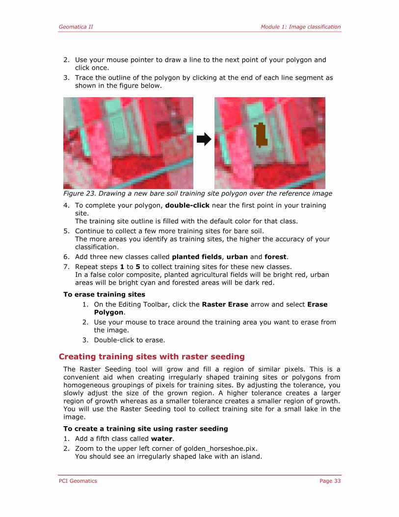
2. Use your mouse pointer to draw a line to the next point of your polygon and
click once.
3. Trace the outline of the polygon by clicking at the end of each line segment as
shown in the figure below.
Figure 23. Drawing a new bare soil training site polygon over the reference image
4. To complete your polygon, double-click near the first point in your training
site.
The training site outline is filled with the default color for that class.
5. Continue to collect a few more training sites for bare soil.
The more areas you identify as training sites, the higher the accuracy of your
classification.
6. Add three new classes called planted fields, urban and forest.
7. Repeat steps 1 to 5 to collect training sites for these new classes.
In a false color composite, planted agricultural fields will be bright red, urban
areas will be bright cyan and forested areas will be dark red.
To erase training sites
1. On the Editing Toolbar, click the Raster Erase arrow and select Erase
Polygon.
2. Use your mouse to trace around the training area you want to erase from
the image.
3. Double-click to erase.
Creating training sites with raster seeding
The Raster Seeding tool will grow and fill a region of similar pixels. This is a
convenient aid when creating irregularly shaped training sites or polygons from
homogeneous groupings of pixels for training sites. By adjusting the tolerance, you
slowly adjust the size of the grown region. A higher tolerance creates a larger
region of growth whereas as a smaller tolerance creates a smaller region of growth.
You will use the Raster Seeding tool to collect training site for a small lake in the
image.
To create a training site using raster seeding
1. Add a fifth class called water.
2. Zoom to the upper left corner of golden_horseshoe.pix.
You should see an irregularly shaped lake with an island.

Module 1: Image classification Geomatica II
Page 34 PCI Geomatics
3. On the Editing toolbar, click the New Shapes arrow and select Raster Seeding.
The Seed Polygon window opens.
Figure 24. Raster Seeding window
4. As the Selection Criteria, select Classification Input.
5. Enter an Input Pixel Value Tolerance of 7.
This will grow the seeded polygon to all pixel values within +/- 7 brightness
values of the original selected pixel.
6. For Neighborhood, select 4 Connect.
This seeds values on all sides, while 8 connect seeds diagonal pixels as well.
7. With the Raster Seeding window open, click inside the lake.
The Raster Seeding tool highlights a group of similar pixels to form a training
site for water.
8. Collect several training sites using the Raster Seeding tool on a few of the other
small lakes in the imagery.
You may have to adjust the tolerances in the Raster Seeding window to get the results you desire.
To collect training sites on Lake Ontario
Use either the Polygon or Rectangle options from the New Shapes tool to
collect training sites over Lake Ontario.
Changing training site colors
Focus automatically assigns colors to new training classes. Planted fields may
appear blue and urban areas may appear yellow when they are drawn in the image
view area. You can change the color of a training site to any color you wish.
To change the color for a training site
1. In the Training Site Editing table, click the color sample for the training site you
want to change.
A color adjustment window opens for the training site you selected.

Geomatica II Module 1: Image classification
PCI Geomatics Page 35
2. In the Basic Colors palette, click a color.
Fine adjustments to the color can be made using the Color Continuum and the
Intensity Scale.
3. Choose a color model from the Models list.
You can choose from four color models: Gray, RGB, CMYK, or HLS/IHS.
4. When you have finished adjusting your training area color, click OK.
The color adjustment window closes, and your new color appears in the Training
Site Editing table.
Lesson summary
In this lesson you:
Created training sites manually
Created training sites using raster seeding
Changed the color of your training sites
Module 1: Image classification Geomatica II
Page 36 PCI Geomatics
Lesson 1.5 - Analyzing training sites
In this lesson you will:
Examine signature statistics
Display class histograms
Evaluate signature separability
Examine scatter plots
Preview the classification
Training site analysis
Often during classification, unique spectral classes appear that do not correspond to
any of the information classes that you want to use. In other cases, a broad
information class may contain a number of spectral sub-classes with unique
variations. This can be caused by a mixture of ground cover types within your
training areas or by shadows and variations in scene illumination. Focus offers
several methods for insuring that your training sites are both representative and
complete. You can analyze your training site data before running the classification
by examining signature statistics, histograms, signature separability and scatter
plots.
Signature statistics
The Signature Statistics window displays the number of samples in the training
area indicating whether you have collected enough pixels to accurately represent
the land cover. In general, if you are classifying n bands, then you require a
minimum of 10n pixels of training data for each class. The General report lists the
mean and standard deviation in each input channel for the pixels within the training
areas of the selected class.
To view your signature statistics
1. In the Training Site Editor, right-click bare soil and select Statistics.
The Signature Statistics window opens.

Geomatica II Module 1: Image classification
PCI Geomatics Page 37
Figure 25. Signature Statistics window
2. In the Signature Statistics window, click another class in the table.
The statistics are automatically displayed for the selected class.
Histograms
You can view and test the reliability of your training sites by creating a histogram in
the Class Histogram window. The histogram shows the frequency of training site
pixels as a percentage of the number of pixels in your training sites. Your histogram
should have a uni-modal shape displaying a single peak. A multi-modal histogram
indicates the likelihood that the training sites for that class are not pure, but
contain more than one distinct land cover class.
Next, you will display a histogram to check the reliability of your training sites.
To create a histogram for a training site
1. From the Tools menu in the Training Site Editor window, select Histogram.
Alternatively, you can select a class, right-click and select Histogram.
The Class Histogram Display window opens, showing a histogram for the bare
soil training site.

Module 1: Image classification Geomatica II
Page 38 PCI Geomatics
Figure 26. Class Histogram Display for bare soil
The x-axis in the histogram represents the gray level value for the image channel
with a range of 0 to 255. The y-axis shows the frequency count as a percentage of
the total count of pixels in the training area corresponding to the gray value.
Signature separability
Signature Separability is calculated as the statistical difference between pairs of
spectral signatures. You can use the Signature Separability window to monitor the
quality of your training sites. Divergence is shown as both Bhattacharrya Distance
and Transformed Divergence, with the Bhattacharrya Distance as the default
calculation.
To open the Signature Separability window
2. From the Tools menu in the Training Site Editing window, select Signature
Separability.
The Signature Separability window opens.

Geomatica II Module 1: Image classification
PCI Geomatics Page 39
Figure 27. Signature Separability window
Both Bhattacharrya Distance and Transformed Divergence are shown as real values
between zero and two. A zero indicates complete overlap between the signatures of
two classes and two indicates a complete separation between the two classes.
These measurements are monotonically related to classification accuracies. The
larger the separability values are, the better the final classification result will be.
Values between 1.9 and 2.0 are considered to indicate good separability.
Scatter plot
You can use the Scatter Plot window to show elliptical graphs for all training sites. A
class ellipse shows the maximum likelihood equiprobability contour defined by the
class threshold value entered for the mean.
Next, you will use the plot Ellipses tool to assess the separability of your spectral
classes and to refine and edit your training statistics.
To display a scatter plot
1. From the Tools menu in the Training Site Editing window, select Scatter Plot.
The Scatter Plot window opens.

Module 1: Image classification Geomatica II
Page 40 PCI Geomatics
Figure 28. Scatter Plot window
2. For each class, select both the Plot Mean and Plot Ellipse option.
Try plotting different band combinations. If you find there is overlap in the
hyperellipses between two or more classes in all band combinations, you may wish
to go back and edit your original training sites. Overlap indicates there may be
confusion between the classes in the final classified image.

Geomatica II Module 1: Image classification
PCI Geomatics Page 41
Note To zoom the scatter plot, right-click inside the graph area
and choose Zoom In. You can also zoom by outlining a
part of the scatter plot with your mouse.
Previewing the classification
The Classification Preview shows how the input channels will be classified using the
training sites and class parameters contained in the training channel. You can also
modify these training site statistics by adjusting the Threshold and Bias.
To preview the classification
From the Tools menu in Training Site Editing window, select Classification
Preview and then select Maximum Likelihood.
Threshold is a relative measure used to control the radius of the hyperellipse for
each class. By changing the threshold values, you can reduce the chances of pixels
being classified into more than one class.
To adjust the Threshold value
1. In the Training Site Editing table, under the Threshold column for the urban
class, type 2.5.
In the Scatter Plot window, the class ellipse for urban adjusts automatically to
show the change in the threshold value. Your Classification Preview also
updates to reflect the change.
2. In the Threshold column for the bare soil class, type 4.
The size of the class ellipse for bare soil increases and the preview updates as
well. There are now more areas classified as bare soil.
3. When you are finished examining the preview, set the Threshold for all classes
back to the default value of 3.
Note Bias is a value from 0 to one, where higher values weigh
one class in favor of another. It can also be used to
resolve overlap between classes. You can use both
Threshold and Bias to test training site separability.
4. Click Save & Close.
You have now saved your training sites and your classification preview has
closed. You are now ready to run your supervised classification.
Lesson summary
In this lesson you:
Examined signature statistics
Displayed class histograms
Evaluated signature separability
Examined scatter plots
Previewed the classification

Module 1: Image classification Geomatica II
Page 42 PCI Geomatics
Lesson 1.6 - Running a supervised classification
In this lesson you will:
Run your supervised classification
Generate a classification report
Now that you have analyzed the reliability of your training sites and tested their
separability, you can run the classification from the Focus Maps tree.
To run your classification
1. In the Maps tree, right-click the Classification MetaLayer and select Run
Classification.
The Supervised Classification window opens.
You can choose from three supervised classification algorithms: Minimum
Distance, Parallelepiped, and Maximum Likelihood.
Figure 29. Supervised Classification window
2. In the Algorithm section, select Maximum Likelihood.
3. In the Classify Options section, choose Show Report.
Note To compare this classification with another classification,
you should also select the Create PCT option. Creating a
Pseudo Colour Table (PCT) will allow you to use the same
colors to display these classes outside of the classification
session.
4. Click OK.
The supervised classification appears in the Focus view area and a Classification
Report window opens showing a report of the completed classification.

Geomatica II Module 1: Image classification
PCI Geomatics Page 43
Your report should show a high overall training site accuracy. The information from
each pixel in the training areas is compared to the information determined by the
classifier algorithm. The overall accuracy represents the percentage of training area
pixels that were correctly classified.
In the next lesson you will examine tools for post-classification analysis.
Lesson summary
In this lesson you:
Ran a supervised classification
Generated a classification report

Module 1: Image classification Geomatica II
Page 44 PCI Geomatics
Lesson 1.7 - Assessing classification accuracy
In this lesson you will:
Generate a random sample of points
Assign a reference class to each point
Produce an accuracy report
Accuracy assessment
Accuracy assessments determine the correctness of the classified image, which is
based on pixel groupings. Accuracy is a measure of the agreement between a
standard that is assumed to be correct and an image classification of unknown
quality. If the image classification corresponds closely with the standard, it is said
to be accurate.
There are several different ways in which accuracy assessments can be
accomplished. One method is to compare the classified image to a reference image.
A random set of points is generated and classification results are compared with the
true information classes in the reference image.
A second method to perform accuracy assessment involves using a GPS. Again, a
random set of points is generated over the classified image. Ground truthing would
be performed by going into the field at the location of each randomly generated
point. The classification results would then be compared to actual land cover at
each point’s location.
It is important to make sure that the reference dataset, be it a reference image or
GPS points, was acquired approximately at the same time of year as the imagery in
order to make a fair comparison.
In this example, you will compare the classified image to a color composite of
golden_horseshoe.pix.
To set up for accuracy assessment
1. From the Maps tree, right-click the Classification MetaLayer and click Post-
classification Analysis and then click Accuracy Assessment.
The Accuracy Assessment window opens.

Geomatica II Module 1: Image classification
PCI Geomatics Page 45
Figure 30. Accuracy Assessment window
2. Click Select Classified Image.
3. In the Select Classified Image window, select channel 10 and click OK.
The classes are loaded under the Assign Reference Class to Sample section.
4. Click Load Reference Image.
5. Load a false color composite by clicking channels 4, 3 and 2 and click OK.
A false color composite is loaded in the view area.
Next, a random sample of points will be generated for the dataset.
To generate a random sample of points
1. On the Accuracy Assessment window, click Generate Random Sample.
The Generate Random Samples window opens.
Figure 31. Generate Random Samples window
2. For the Number of samples, enter 50.
3. Enable the Stratify Samples to class percentages option.
This will randomly choose the number of samples from each class that are
proportional to the percentage of the image occupied by each class. In other
words, larger classes contain more samples than smaller classes.

Module 1: Image classification Geomatica II
Page 46 PCI Geomatics
4. Click OK.
The Random Sample List is populated in the Accuracy Assessment window and a
Random Sample vector point layer is added to the Accuracy Assessment
MetaLayer in the Maps tree.
You will now assign one of the five classes to each point using the Landsat
image as your reference.
To assign a class to each point
1. In the Accuracy Assessment window, select the first sample in the Random
Sample List.
2. Zoom into the image at a resolution of 1:1 or higher.
The selected point is visible in the view area and is surrounded by a green
square. You need to determine which information class this pixels falls on by
using the colors in the reference image as your guide.
3. Select the class in the Assign Reference Class to Sample table to which you
think the random sample belongs.
The Class and Name fields are populated accordingly in the Random Sample
List. The second point is selected automatically.
4. Continue to assign classes to the remaining points in the Random Sample List.
Figure 32. Accuracy Assessment window with each point assigned a class
To save your random sample
1. In the Accuracy Assessment window, click Save.
A New Item Detected window opens.
2. In the File list, select golden_horseshoe.pix.
3. Click Save.
The random sample points and their assigned reference classes are saved to
golden_horseshoe.pix as a point vector layer.

Geomatica II Module 1: Image classification
PCI Geomatics Page 47
Producing an accuracy report
Once reference classes are assigned to the random samples, you can generate an
accuracy report. Accuracy is determined by comparing the assigned reference value
for each test pixel to the category in the classification image. To generate a report,
it is not necessary to assign a reference class to every random sample; however, a
classified image must be previously selected.
The Accuracy Report window creates three types of reports:
Sample Report Listing
Shows which samples are correctly classified.
Error (Confusion) Matrix
Displays the results of the accuracy assessment process. Reference data listed in the columns of the matrix represents the number of correctly classified samples.
Accuracy Statistics
Lists different statistical measures of overall accuracy and accuracy for each class.
To produce an Accuracy Report
1. On the Accuracy Assessment window, click Accuracy Report.
The Accuracy Report window opens.
2. On the Sample Report Listing tab, click Generate Report.
The list of the random samples is displayed showing the georeferenced
position, database position, classified value and reference value of each
point.
3. Click the Error (Confusion) Matrix tab.
4. Click Generate Report.
The values for calculating errors of omission and commission are listed in
the columns and rows, respectively.
5. Click the Accuracy Statistics tab.
6. Click Generate Report.
The Overall Accuracy, Kappa Statistic, Producer’s Accuracy and User’s
Accuracy are calculated.
Note For the Error (Confusion) Matrix and the Accuracy
Statistics, a 3x3 mode filter can be applied to the
classified values.
Lesson summary
In this lesson you:
Generated a random sample of points
Assigned a reference class to each point
Produced an accuracy report

Module 1: Image classification Geomatica II
Page 48 PCI Geomatics
Lesson 1.8 - Post-classification filtering and vectorization
In this lesson you will:
Apply a mode filter to a classified image
Apply a sieve filter to a classified image
Vectorize a thematic raster layer
Post-classification filtering of image data is used to remove any unwanted noise
from a thematic dataset. Filtering will generalize the dataset removing stray pixels
in the image producing more homogenous class areas.
Two common methods for post-classification processing are mode filtering and
sieve filtering. A mode filter computes the mode (most frequently occurring gray-
level value) within the filter window. A sieve filter gives more control over the
filtering process by allowing a threshold to be specified for the smallest polygon not
to be merged into a neighbor.
Once the classified image has been filtered, vectors can be created for the dataset.
A raster dataset is thus vectorized so each polygon contains the class information
from the classified image.
To set the Input and Output Ports for FMO
1. From the Tools menu, open the Algorithm Librarian and double-click
FMO
The FMO Module Control Panel opens

Geomatica II Module 1: Image classification
PCI Geomatics Page 49
Figure 33. FMO Module Control Panel
2. For the Input Unfiltered Layer, select channel 10
3. In the Output Ports section, clear the check mark from the Viewer-
Grayscale option
4. Select the Viewer-PCT option.
To set the Input Parameters and run FMO:
1. On the FMO Module Control Panel, click the Input Params 1 tab.
2. For Thin Line Preservation, select ON

Module 1: Image classification Geomatica II
Page 50 PCI Geomatics
Figure 34. FMO Input Parameters
3. Click Run
4. Click Close
The mode filtered image is displayed in the view area. The filtered image
maintains the class metadata that was part of the original dataset. Test
the effects of using a larger filter size on the results.
To set the Input and Output Ports for SIEVE
1. From the Algorithm Librarian, double-click SIEVE
The SIEVE Module Control Panel opens.

Geomatica II Module 1: Image classification
PCI Geomatics Page 51
Figure 35. SIEVE Module Control Pane
2. For the Input Raster Layer, select channel 10.
3. In the Output Ports section, clear the check mark from the Viewer-
Grayscale option.
4. Select the Viewer-PCT option.
To set the Input Parameters and run SIEVE
1. On the SIEVE Module Control Panel, click the Input Params 1 tab.
2. For the Polygon Size Threshold, enter 6.
3. Click Run.
4. Click Close.
The sieve filtered image is displayed in the view area. The filtered image
maintains the class metadata that was part of the original dataset.
Visually compare the results of FMO and SIEVE.

Module 1: Image classification Geomatica II
Page 52 PCI Geomatics
Next, you will run RAS2POLY to vectorize a classified image. The
thematic_raster.pix file contains a classified image layer that has been filtered with
a 7x7 mode filter. Additionally, RAS2TMR was run on the raster layer to create a
thematic raster layer.
To start a new project and load a new file
1. On the Focus toolbar, click New Project.
2. From the GEOII Data folder, open t_raster.pix.
A pseudocolor image opens in the view area.
To set the Input and Output Ports for RAS2POLY
1. From the Algorithm Librarian, double-click RAS2POLY.
2. For the Input Raster Layer, select channel 1.
3. In the Output Ports section, select the Untitled.pix option.
4. Right-click Untitled.pix and click Browse.
5. From the GEOII Data folder, select t_raster.pix and click Save.
Figure 36. Input and Output options for RAS2POLY
6. Click Run.
The default input parameter of whole polygons will be used. The output
vector layer is saved to t_raster.pix and is also displayed in the view area.

Geomatica II Module 1: Image classification
PCI Geomatics Page 53
Lesson summary
In this lesson you:
Applied a mode filter to a classified image
Applied a sieve filter to a classified image
Vectorized a thematic raster layer


PCI Geomatics Page 55
Module 2: DEM Editing in Focus
About this module
Module 2 has three lessons:
Lesson 2.1 – Quality Assessment Tools
Lesson 2.2 – Editing a DEM to compensate for Roads, Bridges or Overpasses
DEM Editing
A Digital Elevation Model, or DEM, is a gridded array of elevation values. A DEM can
be derived from many different sources; such as contour lines, Triangular Irregular
Networks (TINs), or stereo images. When a DEM is extracted from stereo image
pairs, the un-edited result is often referred to as a Digital Surface Model or DSM
because it represents surface heights (the height at the tops of trees, buildings
etc.) and not ground heights. When a DSM has been edited to remove the heights
of features like trees, or buildings, the resulting product is usually referred to as a
Digital Terrain Model or DTM because it reflects the ground heights and not the
height of the ground plus an object.
Satellite imagery and aerial photographs contain inherent distortions from
topographical variations and sensor geometry. The orthorectification process
removes distortions in images providing images with a constant scale, with features
in their correct Cartesian positions. An orthorectified image permits a user to obtain
accurate measurements of distances, angles and areas. A DEM plays an integral
role in the orthorectification process and therefore using an accurate DEM is
paramount when correcting distortions in raw satellite and aerial images.
The three lessons in this module will examine different aspects and tools that are
available in Focus for DEM editing.
Lesson 2.1 Quality Assessment Tools In this lesson you will:
Use FLY! to aid in denoting areas that require editing
Use full resolution update ortho to assess the quality of the extracted DEM
Geomatica FLY!
“Geomatica FLY!” provides a different 3D viewing perspective that is not possible in
Focus. This different perspective aids in image interpretation that assists in the
DEM editing process. In this exercise, you will use “FLY!” to familiarize yourself with
the image data that is draped over the extracted un-edited DSM.

Module 2: DEM Editing in Focus Geomatica II
Page 56 PCI Geomatics
Using “FLY!” before you perform any DEM editing tasks allows you to focus on the
elements of the DEM that require special attention before you apply any filtering to
the DEM.
To launch FLY! for DEM interpretation
1. Launch Geomatica Focus
2. In the Focus “Files” treelist, right select “Add”
3. Browse to the “DEM-Editing” folder within the GeoII training folder
4. Select the “QuebecCity_DSM_GeoII.pix” file located in the DSM folder and
click “Open”
The file appears in the Focus “Files” treelist.
Figure 37. DEM in Files Treelist
5. Expand the Rasters layer by clicking on the + symbol
6. Right select the 32R extracted DEM and select View | As Grayscale
The image is loaded to the Maps treelist and canvas
7. Select the “QuebecCity_DSM_GeoII.pix” layer in the Maps Treelist
8. With the layer highlighted, select “Layer | DEM editing”
The grayscale image is replaced with a shaded-pseudo color image and the DEM
editing panel is launched.

Module 2: DEM Editing in Focus Geomatica II
PCI Geomatics Page 57
Figure 38. Extracted DSM loaded in Focus
9. On the DEM editing window, click “Open Fly!” to launch FLY!
FLY! is launched and the aerial photographs are draped overtop the extracted
DSM.

Module 2: DEM Editing in Focus Geomatica II
Page 58 PCI Geomatics
Figure 39. Geomatica FLY! with aerial photos draped over DSM
To change the viewing direction in FLY!
10. Use the mouse left button and click anywhere in the FLY! viewer.
The view will be automatically updated, centered on the cursor location.
To fly over the draped imaged
11. Click the “Free flight” button on the main FLY! window (2nd from left)
To stop flying over the draped imaged
12. Click the “Free flight” button
To control the speed and flying altitude above the photos
13. Use the FLY! Control Panel (1st button on main FLY! window)
Increase or decrease elevation
Increase or decrease speed
Exercise:
Take notes of areas that may require special consideration (highways and overpasses).

Module 2: DEM Editing in Focus Geomatica II
PCI Geomatics Page 59
Full Resolution Ortho Preview
Another Quality Assessment tool is the full resolution ortho preview window. This
tool will help you understand the imagery that is draped over the DEM. It provides
you with a view of the ortho-imagery that will be generated with the current edits
applied to a DEM. The full resolution ortho window also provides you with access to
all of the images that overlap that defined area.
To open the Full resolution Ortho Preview window
1. Click the Define Preview region button on the main DEM editing panel
2. Move your mouse over the Focus viewing canvas
3. With your mouse, drag out a rectangular box
The full resolution window is launched
A progress monitor appears indicating the status of the live orthorectification
process
Figure 40. Full resolution ortho preview window
Exercise:
Randomly open the full resolution ortho preview for different areas of the DEM and take notes of any anomalies that require special consideration.
Lesson summary
In this lesson you:

Module 2: DEM Editing in Focus Geomatica II
Page 60 PCI Geomatics
Used FLY! to mark areas in the DSM that required editing
Used the full resolution update ortho-image to detect areas in the DSM
needing improvement.
Lesson 2.2 Editing roads, Bridges or Overpasses
In this lesson you will:
Edit roads, bridges or Overpasses in a DEM
A DTM or DEM used for orthorectification typically contains terrain heights and has
surface heights removed. Doing so provides a more geographically accurate ortho-
image. One special exception that cannot be applied to this general rule is a bridge,
or overpass. If the elevation values for a bridge are not at the bridge height, then
during the orthorectification process the bridge will be stretched downwards toward
the ground. This stretching will make the bridge appear in the incorrect location (as
well as have a distorted appearance).
In order to fix a bridge (or highway overpass) you will need to find one that is
broken or distorted in the image. Use your notes from Lesson 2.1 to focus on one
particular bridge.
Fixing a bridge involves a four step process; first, digitize stabilizer polygons on two
opposite ends of the bridge; two, apply a terrain filter to remove the bridge (except
the areas used as stabilizers); three, to digitize the bridge; and four to apply an
opposite ends filter to restore the bridge.
To Digitize bridge stabilizers
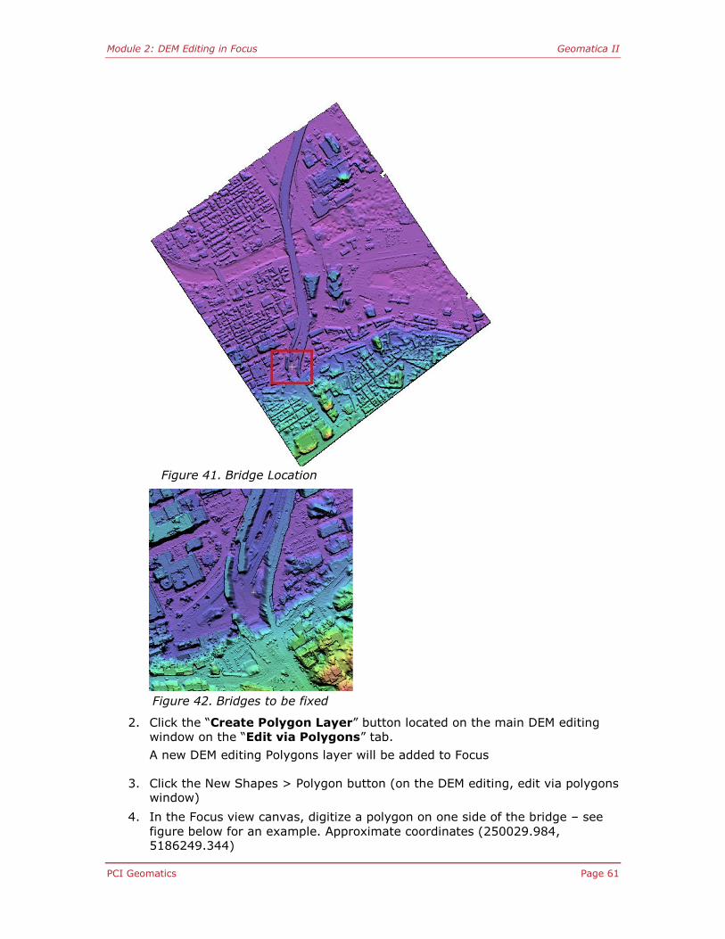
1. Zoom to a bridge you made note of in Lesson 2.1 that requires fixing. Or,
zoom to the bridge seen in Figure 41 Bridge Location below
Module 2: DEM Editing in Focus Geomatica II
PCI Geomatics Page 61
Figure 41. Bridge Location
Figure 42. Bridges to be fixed
2. Click the “Create Polygon Layer” button located on the main DEM editing
window on the “Edit via Polygons” tab.
A new DEM editing Polygons layer will be added to Focus
3. Click the New Shapes > Polygon button (on the DEM editing, edit via polygons window)
4. In the Focus view canvas, digitize a polygon on one side of the bridge – see
figure below for an example. Approximate coordinates (250029.984, 5186249.344)

Module 2: DEM Editing in Focus Geomatica II
Page 62 PCI Geomatics
It may be necessary to adjust your snap tolerance settings (Tools > Options
> Vector Editing) if you are having difficulty drawing the polygon. The default
snap tolerance is 5 screen pixels.
Figure 43. First bridge stabilizer
5. Repeat for the other side of the bridge (see figure below) – Approximate
coordinates (250049.934, 5186545.744)
Figure 44. Second bridge stabilizer
6. Create additional stabilizer polygons for each bridge within the vicinity that will be fixed.
Your polygons should look something like this:
Module 2: DEM Editing in Focus Geomatica II
PCI Geomatics Page 63
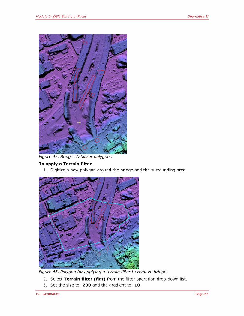
Figure 45. Bridge stabilizer polygons
To apply a Terrain filter
1. Digitize a new polygon around the bridge and the surrounding area.
Figure 46. Polygon for applying a terrain filter to remove bridge
2. Select Terrain filter (flat) from the filter operation drop-down list.
3. Set the size to: 200 and the gradient to: 10

Module 2: DEM Editing in Focus Geomatica II
Page 64 PCI Geomatics
4. Click Apply
The DEM should now appear like this:
Figure 47. Applied Terrain filter with Stabilizer polygons
5. Delete the polygons (including the stabilizer polygons)
To Digitize the bridge
1. Zoom to a starting location (near where a stabilizer polygon was located)
2. Digitize the west most bridge
Use the “Display DEM” button to display the low-resolution image. Remember
not to follow the exact bridge outline as the original DEM contained errors and
the bridge in the low-res ortho is distorted.
Your new bridge should look something like this:

Module 2: DEM Editing in Focus Geomatica II
PCI Geomatics Page 65
Figure 48. Digitized bridge vector overlapping image and DSM
To apply an Opposite ends filter
1. Select the bridge polygon shape
Select “Opposite ends fill (blend ends only)” from the filtering operations
drop-down menu
2. Click “Apply”
The DEM is updated and the bridge is now restored in the DSM. It is a good
idea to check the quality of the restored bridge and fine tune the bridge
polygon if needed.
To check the quality and find tune the bridge polygon
1. Open the full resolution preview window
2. Click on the “Left” image drop-down and select “L Ortho 4”
3. Zoom to 1:1 (1 to 1) resolution
4. Use the reshape tool in the Full Res. Ortho Preview window to fix the bridge
polygon
5. Close the full-res Ortho preview window
6. Click “Apply” (to fill from opposite ends on the reshaped bridge polygon).
Module 2: DEM Editing in Focus Geomatica II
Page 66 PCI Geomatics
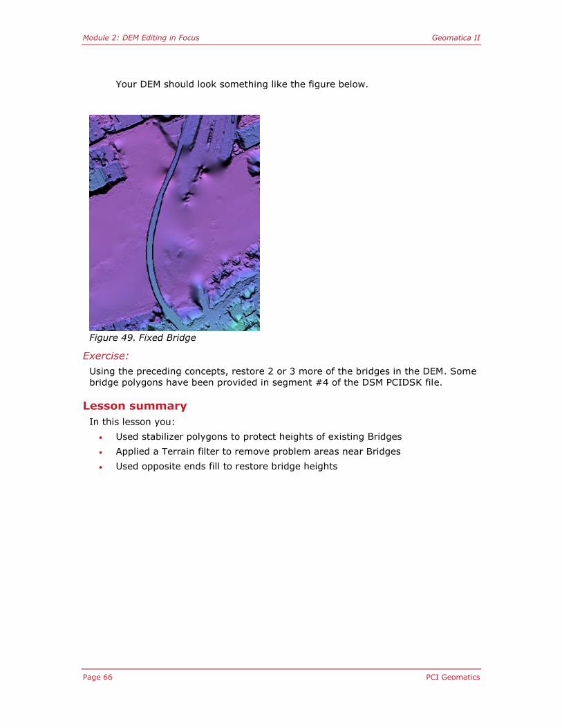
Your DEM should look something like the figure below.
Figure 49. Fixed Bridge
Exercise:
Using the preceding concepts, restore 2 or 3 more of the bridges in the DEM. Some
bridge polygons have been provided in segment #4 of the DSM PCIDSK file.
Lesson summary
In this lesson you:
Used stabilizer polygons to protect heights of existing Bridges
Applied a Terrain filter to remove problem areas near Bridges
Used opposite ends fill to restore bridge heights
Module 3: Spatial analysis in Focus Geomatica II
PCI Geomatics Page 67
Module 3: Spatial analysis in Focus
About this module
Module 3 has six lessons:
Lesson 3.1 - Buffering vectors
Lesson 3.2 - Dissolving vectors
Lesson 3.3 - Finding area neighbors
Lesson 3.4 - Performing a spatial overlay
Lesson 3.5 - Performing a statistical overlay
Lesson 3.6 - Performing a suitability overlay
Spatial analysis
A variety of Focus tools are provided for working with spatial analysis components for your project.
This module provides information for preparing input data, managing data
attributes, exporting data, working with data properties, and working with vector and raster data.
Lesson 3.1 - Buffering vectors
In this lesson you will:
Create a buffer around existing vectors
Creating buffers
A buffer is a margin created at a specific distance around shapes on a layer. You
can create margins of different sizes, each referred to as a buffer level. You use
buffer levels to analyze suitability or risk around the input shapes, which is referred
to as a proximity analysis. Buffers can be created for lines, points and polygons.
For example, you can create a buffer around domestic wells to analyze the risk of contamination from pesticide use.
In this lesson you will use the roads layer in the california.pix file to create a buffer
around major highways to identify zones for the cost-effective transportation of goods.
To open the Roads vector layer
1. Start a new project in Focus.
2. In the Focus window, select the Files tree.
3. Right-click in the Files tree and select Add.
A File Selector window opens.

Module 3: Spatial analysis in Focus Geomatica II
Page 68 PCI Geomatics
4. From the GEOII Data folder, open california.pix.
The california.pix file is listed in the Files tree as part of your project, but
the data is not loaded into the viewer. This allows you to select which
layer you wish to view.
5. From the list of vectors, right-click the Roads layer and select View.
The Roads layer is loaded into the viewer and is listed in the Maps tree.
To launch the Buffer Wizard
1. From the Analysis menu, select Buffer.
The Buffer Wizard opens.
Figure 50. Buffer Wizard
To set up the Data and Size for the buffer
1. For the input File, select california.pix.
2. For the input Layer, select 7 [VEC] Arcs:Roads.
Note If the layer you want to buffer is selected in the Maps
tree, you can apply the buffer to the Active Layer.
3. For Output, select the Display option.
The results will be displayed in the viewer only and not saved to a file.

Module 3: Spatial analysis in Focus Geomatica II
PCI Geomatics Page 69
Note If vectors are selected in the active vector layer before
opening the Buffer Wizard, you have the option to apply
the buffer to the selected vectors only by clicking the
Buffer selected shapes only option.
4. For the Buffer Distances option, select Field.
5. From the attribute list box, select roadtype.
This will buffer the shapes according to this attribute.
6. In the Buffer levels list, enter 2.
You can create multiple buffers around an object with the Buffer levels
option. The number you specify creates the same number of Level
columns in your Buffer Distances table. You can then enter a different
buffer size for each level.
7. In the Units list, select Km.
8. For the Major Highway road type, enter a value of 2 in the Level1 column
and a value of 4 in the Level2 column.
Figure 51. Buffer Wizard for Roads layer
9. Click Next.
The second window opens where you can select your vertex, line,
polygon, attribute and output options.

Module 3: Spatial analysis in Focus Geomatica II
Page 70 PCI Geomatics
To set up the Output Options
1. In the Vertex Options section, select Round.
2. For the Line Options, select Both sides.
3. For the End style, select Round.
4. For the Fields to Add, select the SourceShapeID and BufferLevel
options.
5. For the Output Areas, select Combine.
6. Click Finish.
The output is a Temporary Vector Layer displaying all areas within a 2 km
and a 4 km buffer of the major highways in the roads layer.
Figure 52. Buffer Results
Now that you have created the buffer layer and you are satisfied with the results, you can save the output to a new file.
To save the Temporary Vector Layer
1. In the Maps tree, right-click the Temporary Vector Layer and select Save
As.
The Save As window opens.

Module 3: Spatial analysis in Focus Geomatica II
PCI Geomatics Page 71
Figure 53. Save As window
2. For the Output File name, click Browse and navigate to the GEO Data
folder.
3. For the File name, type RoadBuffer.pix and click Save.
4. In the Format list, select PCIDSK (.pix).
A new PCIDSK file will be created.
5. In the Layer box, type 2 km and 4 km road buffer.
6. Click Save.
The Save As window closes and both the Maps tree and Files tree are
updated with the new filename and layer description.
Lesson summary
In this lesson you:
Created a buffer around existing vectors

Module 3: Spatial analysis in Focus Geomatica II
Page 72 PCI Geomatics
Lesson 3.2 - Dissolving vectors
In this lesson you will:
Add a new field
Perform a Query by Example
Dissolve coniferous versus non-coniferous shapes
Using Dissolve
Dissolve combines shapes that contain the same value for a selected attribute. The
resulting output is a layer that contains the newly combined shapes with each
shape represented as a layer record. A dissolve can only be performed on polygon
vector layers.
Before you start this lesson, you will remove the data from the previous lesson.
To remove the existing data from the Maps tree
1. In the Maps tree, right-click the Roads layer and select Remove from
Area.
2. Right-click RoadBuffer layer and select Remove from Area.
To open the Vegetation vector layer
1. Click the Files tree.
2. From the list of vectors in the california.pix file, right-click the Vegetation
layer and select View.
The Vegetation vector layer opens in the Focus view area.
This vector layer has embedded representation which displays certain shapes in
green based on their vegetation type. Representation is discussed in Module 4.
In a dissolve, a common attribute is needed as a basis for the dissolve operation.
All features with this common attribute will be dissolved, or merged. In this lesson,
you will dissolve different vegetation types into two categories: coniferous and not coniferous. First, you must add a new field to contain the common attribute.
To add a new field
1. In the Maps tree, right-click the Vegetation vector layer and select
Attribute Manager.
The Attribute Manager for the vegetation layer opens.

Module 3: Spatial analysis in Focus Geomatica II
PCI Geomatics Page 73
Figure 54. Attribute Manager
2. From the Field menu in the Attribute Manager, select Add New.
The Table Definition window opens.
Figure 55. Table Definition window
3. In the Name column, double-click Field7 and type Coniferous.
This new field will indicate whether or not the vegetation is coniferous.
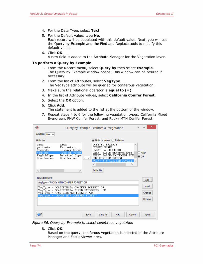
Module 3: Spatial analysis in Focus Geomatica II
Page 74 PCI Geomatics
4. For the Data Type, select Text.
5. For the Default value, type No.
Each record will be populated with this default value. Next, you will use
the Query by Example and the Find and Replace tools to modify this
default value.
6. Click OK.
A new field is added to the Attribute Manager for the Vegetation layer.
To perform a Query by Example
1. From the Record menu, select Query by then select Example.
The Query by Example window opens. This window can be resized if
necessary.
2. From the list of Attributes, select VegType.
The VegType attribute will be queried for coniferous vegetation.
3. Make sure the relational operator is equal to (=).
4. In the list of Attribute values, select California Conifer Forest.
5. Select the OR option.
6. Click Add.
The statement is added to the list at the bottom of the window.
7. Repeat steps 4 to 6 for the following vegetation types: California Mixed
Evergreen, PNW Conifer Forest, and Rocky MTN Conifer Forest.
Figure 56. Query by Example to select coniferous vegetation
8. Click OK.
Based on the query, coniferous vegetation is selected in the Attribute
Manager and Focus viewer area.

Module 3: Spatial analysis in Focus Geomatica II
PCI Geomatics Page 75
Now that all the coniferous vegetation types are selected, you will replace the value of No with a value of Yes for the Coniferous attribute.
To replace attributes in the Attribute Manager
1. From the Edit menu, select Replace.
The Find and Replace window opens.
Figure 57. Find and Replace window
2. In the Find what box, enter No.
3. Select the Limit search to selected records option.
This will perform the search only in the records selected based on the
query.
4. In the Replace with box, enter Yes.
5. Click Replace All.
In the Coniferous field, the default value of No has been replaced with a
value of Yes for the vegetation types selected in the query.
6. Click Close.
Now that you have added and modified a common attribute for the layer, you can
perform the dissolve based on coniferous and non-coniferous vegetation types.
Before dissolving any vectors, ensure any previously selected shapes have been
cleared.
To dissolve the vegetation types
1. From the Analysis menu in the Focus window, select Dissolve.
The Dissolve window opens.
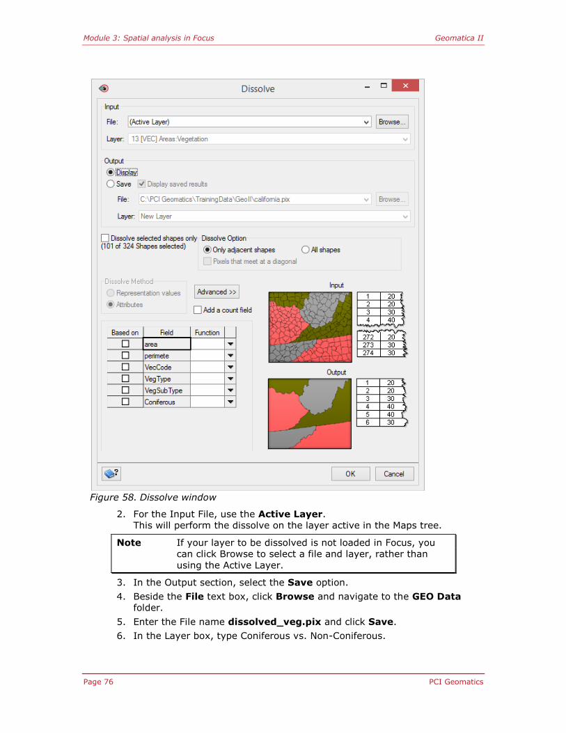
Module 3: Spatial analysis in Focus Geomatica II
Page 76 PCI Geomatics
Figure 58. Dissolve window
2. For the Input File, use the Active Layer.
This will perform the dissolve on the layer active in the Maps tree.
Note If your layer to be dissolved is not loaded in Focus, you
can click Browse to select a file and layer, rather than
using the Active Layer.
3. In the Output section, select the Save option.
4. Beside the File text box, click Browse and navigate to the GEO Data
folder.
5. Enter the File name dissolved_veg.pix and click Save.
6. In the Layer box, type Coniferous vs. Non-Coniferous.
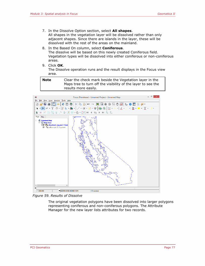
Module 3: Spatial analysis in Focus Geomatica II
PCI Geomatics Page 77
7. In the Dissolve Option section, select All shapes.
All shapes in the vegetation layer will be dissolved rather than only
adjacent shapes. Since there are islands in the layer, these will be
dissolved with the rest of the areas on the mainland.
8. In the Based On column, select Coniferous.
The dissolve will be based on this newly created Coniferous field.
Vegetation types will be dissolved into either coniferous or non-coniferous
areas.
9. Click OK.
The Dissolve operation runs and the result displays in the Focus view
area.
Note Clear the check mark beside the Vegetation layer in the
Maps tree to turn off the visibility of the layer to see the
results more easily.
Figure 59. Results of Dissolve
The original vegetation polygons have been dissolved into larger polygons
representing coniferous and non-coniferous polygons. The Attribute
Manager for the new layer lists attributes for two records.

Module 3: Spatial analysis in Focus Geomatica II
Page 78 PCI Geomatics
Figure 60. Dissolved Vegetation Attribute Manager
Lesson summary
In this lesson you:
Added a new field
Performed a Query by Example
Dissolved coniferous versus non-coniferous shapes

Module 3: Spatial analysis in Focus Geomatica II
PCI Geomatics Page 79
Lesson 3.3 - Finding area neighbors
In this lesson you will:
Find Area Neighbors
Display the resulting attributes in a chart
Area neighbors
Area Neighbors is a reporting tool for determining polygons adjacent to selected
polygons of interest. It can be used for whole polygon layers, topological polygon
layers, and thematic rasters. It generates an unconnected table containing
attributes to analyze the relationship between shapes. For this tool, adjacency is defined as having shared perimeter.
In this example, you will create a table reporting population information for 1970
and 1996 for all counties adjacent to Los Angeles County.
To find Area Neighbors
1. Begin by removing the layers used in the previous lesson from the Maps
tree.
2. In the Files tree, right-click the Counties layer and select View.
3. Using the individual Selection Tool, select Los Angeles County, ShapeID
11.
Figure 61. Los Angeles county
4. From the Focus Layer menu, select Area Neighbors.
The Area Neighbors window opens.

Module 3: Spatial analysis in Focus Geomatica II
Page 80 PCI Geomatics
Figure 62. Area Neighbors window
5. Select Find neighbors to selected input areas only.
Area Neighbors finds neighbors to the selected county polygon.
6. Select the Adjacent to the input areas option.
This reports which shapes border Los Angeles County.
7. In the both the Input Areas column and the Neighbors column, select
ct_name, 1970popu and 1996popu.
This is the information that will be reported in the table for shapes
adjacent to the selected shape.
8. Select the Select Found Neighbors option.
Results of Area Neighbors will be shown graphically.
9. Click OK.
A new table is created.

Module 3: Spatial analysis in Focus Geomatica II
PCI Geomatics Page 81
Figure 63. Area Neighbors Resulting Attribute Manager
The table reports the original ID of the selected polygon (InputId), the polygons
adjacent to the selected polygon (Adj.Id), perimeter information, and because of
the options selected in the ‘Fields to include’ section of the Area Neighbors window,
it also reports the county name (ct_name) and population information for both the
selected polygon and the neighboring polygons.
To save the report
1. From the Layer menu in the Attribute Manager, select Save.
The New Item Detected window opens.
Figure 64. New Item Detected window
2. From the File list, select california.pix.
3. Leave the default settings for Format and Layer.
4. Click Save.
The resulting table is saved as a layer in the california.pix file.

Module 3: Spatial analysis in Focus Geomatica II
Page 82 PCI Geomatics
Viewing data as a chart
Charts are a way to visualize your data. A chart is a table of attributes displayed as
a graphic where the values of selected records and fields are compared. It displays
quantitative data so you can see how the numbers relate to each other, which helps
you to interpret the information more easily. Trends or anomalies may become
evident when displayed using the appropriate chart type. For example, it may be
difficult to identify trends by looking at a table filled with population statistics, but
with the right chart the pattern become easily discernable.
You can create more than one chart per layer. Each chart is connected to the
attributes in the layer so if the attribute values change, the chart changes to reflect the new values.
Now you will create a chart to graphically display population information for 1970
and 1996 for all counties adjacent to Los Angeles County. This could be a good indicator of urban sprawl.
To define the data to chart
1. In the Attribute Manager for the Area Neighbors layer, use the SHIFT key
to select all four records.
The chart will be populated with these selected records.
2. From the Tools menu, select Charts and then Define.
The Chart Definition window opens.
Figure 65. Chart Definition window
3. From the Type list, select Clustered Column.
4. In the Fields list, select Nghbr(1970popu) and Nghbr(1996popu).
The chart is displayed in the Preview section.

Module 3: Spatial analysis in Focus Geomatica II
PCI Geomatics Page 83
5. For the Series in option, select Fields.
Now that you have selected the data to chart, you will design the chart surround to
give meaning to the data displayed in the chart.
To set up the chart surround
1. In the Chart Definition window, click the Options tab.
2. In the Title box, type Population Increase 1970 - 1996.
3. In the Category field list, select Nghbr(ct_name).
4. Click OK.
The Chart Definition window closes and the chart is displayed in the Chart
viewer.
To change the color of the columns
1. In the Chart viewer, click the Selection Tool button.
2. Click one of the columns in the viewer.
Columns for the selected attribute are outlined in green.
3. On the Chart viewer toolbar, click the Color arrow.
4. Select a color from the palette.
5. Repeat step 2 to 4 to change the color for the other attribute.
Your chart should look similar to the one below.
Figure 66. Chart displaying population information

Module 3: Spatial analysis in Focus Geomatica II
Page 84 PCI Geomatics
Charts are kept in memory as long as the project remains open, even if you close the Chart viewer. You can reopen an existing chart by using the Chart Manager.
To open the Chart Manager
1. In the Attribute Manager, click Tools.
2. Select Charts and then Manage.
The Chart Manager opens.
The settings for each chart that you create are saved in the project file (.gpr) when
you save the project. The data itself, however, is not saved with the chart. The
chart only contains a reference to the data. If you make changes to the layer's
attributes, the chart will reflect the changes in the data the next time you open it,
but the design of the chart will remain unchanged. If you close the project without
saving it, the charts in memory are discarded along with any other changes in the project file.
You can also export your chart as a graphic in one of several file formats.
To export the chart
On the Chart viewer toolbar, click Export Chart.
The Export Chart window opens where you can specify a file name and select a format.
Lesson summary
In this lesson you:
Found Area Neighbors
Displayed the resulting attributes in a chart

Module 3: Spatial analysis in Focus Geomatica II
PCI Geomatics Page 85
Lesson 3.4 - Performing a spatial overlay
In this lesson you will:
Combine two layers using a Spatial Overlay
Spatial overlay
Spatial Overlay creates a new layer containing the attributes from two or more
layers. For example, you can overlay a layer containing land-ownership polygons
and a layer containing vegetation polygons to analyze what types of vegetation are located on each property.
In this first example, you will perform a spatial overlay to locate bridges.
To combine layers with a Spatial Overlay
1. Begin by removing the layers used in the previous lesson from the Maps
tree. Ensure the California.pix file remains loaded into the Files treelist.
2. From the Analysis menu, select Overlay.
The Overlay Wizard opens.
Figure 67. Overlay Wizard
The Overlay Wizard contains three overlay types: Spatial Overlay,
Statistical Overlay, and Suitability Overlay.

Module 3: Spatial analysis in Focus Geomatica II
Page 86 PCI Geomatics
3. Select the Spatial option and click Next.
Available input layers are displayed.
Figure 68. Available input for Spatial Overlay
4. In the Available Files/Layers list, enable the check mark beside the Rivers
and Roads layers.
5. Click Next.
6. From the Layer list, select Roads.
The available attributes from the Roads layer are displayed in the Input
Attribute list.
7. From the Input Attribute list, select roadtype and click Add.
This attribute from the roads layer is added to the Output Attributes list. It
is appended with a suffix of _2 indicating it refers to the second input
layer.
Note If you want to change the order of the attributes, select
one in the Attribute table and click the up or down arrow
buttons.
If you want to change the names of an attribute, double-
click it and type a new name.
8. Click Next.

Module 3: Spatial analysis in Focus Geomatica II
PCI Geomatics Page 87
Figure 69. Output Options for Spatial Overlay
9. In the Output Options section, select Union.
Note Union includes all shapes in their entirety from all the
input layers. Intersection includes only the overlapping
areas of the shapes from the input layers.
10. In the Output Layer section, select Points from the Type list.
11. Select the Save option and click Browse.
12. Navigate to the GEO Data folder and type the File name bridges.pix and
click Save.
13. Click Finish.
The Overlay runs and the output is displayed in the viewer.

Module 3: Spatial analysis in Focus Geomatica II
Page 88 PCI Geomatics
Figure 70. Spatial Overlay results
The resulting point layer represents the location of bridges.
If you examine the Attribute Manager for the layer, you will see the IDs of the two
input layers, the union of which indicates the location of a bridge. By including the roadtype attribute, you know the type of road that spans the river.
To view attributes of the spatial overlay output
In the Maps tree, right-click the Spatial Overlay layer and select Attribute
Manager.
The Attribute Manager opens displaying the new attribute information.
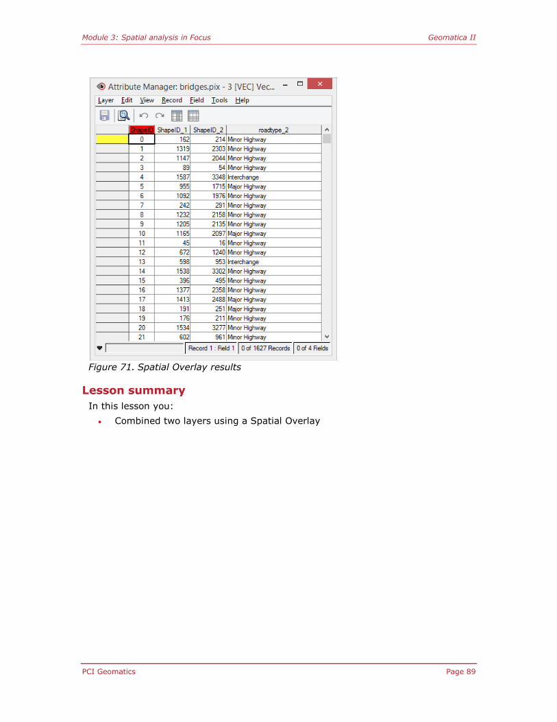
Module 3: Spatial analysis in Focus Geomatica II
PCI Geomatics Page 89
Figure 71. Spatial Overlay results
Lesson summary
In this lesson you:
Combined two layers using a Spatial Overlay

Module 3: Spatial analysis in Focus Geomatica II
Page 90 PCI Geomatics
Lesson 3.5 - Performing a statistical overlay
In this lesson you will:
Transfer attributes from one layer to another
Statistical overlay
Statistical Overlay transfers the selected attributes from one layer to another. It
computes statistics by virtually overlaying two layers. One layer, called the Primary Input, receives the attributes from another layer, called the Secondary Input.
There are two possible results when you transfer attributes between the layers:
Each shape in the Primary Input can receive the attributes from one shape in
the Secondary Input. For example, you can transfer the county attributes
from a county layer to a cities layer. Each city in the Primary Input receives the attributes from the county that contains the city.
Each shape in the Primary Input can receive the attributes from many shapes
in the Secondary Input. You must specify a function to aggregate the
attributes from the Secondary Input. For example, you can transfer the city
attributes from a cities layer to a county layer. Each county in the Primary
Input receives the sum of the population of the cities contained within that county.
To transfer attributes to another layer
1. Begin by removing the layers used in the previous lesson from the Maps
tree.
2. From the Analysis menu, select Overlay.
The Overlay Wizard opens.
3. Select the Statistical option and click Next.

Module 3: Spatial analysis in Focus Geomatica II
PCI Geomatics Page 91
Figure 72. Selecting Input for Statistical Overlay
4. In the Primary Input section, select california.pix from the File list.
5. From the Layer list, select Counties.
This is the layer that will receive the new attributes.
6. In the Secondary Input section, click Browse and select bridges.pix from
the GEOII Data folder.
This is the vector layer that contains the attributes you want to add to the
Primary Input layer.
7. Click Next.
8. Select the Count option.
When you select the Count option, Focus calculates the number of shapes
combined to form each record and adds that attribute to the output layer.
Note You can add several new fields per attribute by clicking
Advanced.
9. Click Finish.
The Attribute Manager for the Counties layer opens automatically. Listed
as the last column in the table is the number of bridges in each county
(OverlayCount).

Module 3: Spatial analysis in Focus Geomatica II
Page 92 PCI Geomatics
Figure 73. New attributes added after Statistical Overlay
Lesson summary
In this lesson you:
Transferred attributes from one layer to another

Module 3: Spatial analysis in Focus Geomatica II
PCI Geomatics Page 93
Lesson 3.6 - Performing a suitability overlay
In this lesson you will:
Convert polygon data to raster data
Assign attribute weights
Perform the Suitability Overlay
Suitability overlay
Suitability Overlay analyzes the relative importance of input layers and attributes to
identify areas that produce the most positive result.
To perform the analysis, you must build a project containing thematic raster layers
that you want to use in the calculation. Each layer should contain one type of data
representing a factor in the calculation. For example, if you are trying to determine
the best location for a winery, your project could contain a layer with rainfall for an
area, a layer of soil types found in the area, a layer containing the road network, and so on.
To calculate a combination that produces the best result, you must decide on a
scale to rank the importance of the layers and a scale to rank the data in the
layers. The scales measure the relative importance of each input into the equation;
the most important factors affect the results the most. The value from the scale that you assign to the layer and to the data is called a weight.
You will begin by opening the RoadBuffer.pix file you created in a previous lesson
and converting it from vector to raster.
To convert from a vector polygon layer to a raster layer
1. From the GEOII Data folder, open RoadBuffer.pix.
2. From the Tools menu, select Algorithm Librarian.
The Algorithm Librarian opens.
3. In the Algorithm Library list, expand the Spatial Analysis folder then the
Conversion tools folder.
4. Select POLY2RAS and click Open.
The POLY2RAS Module Control Panel opens.
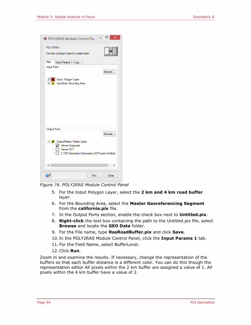
Module 3: Spatial analysis in Focus Geomatica II
Page 94 PCI Geomatics
Figure 74. POLY2RAS Module Control Panel
5. For the Input Polygon Layer, select the 2 km and 4 km road buffer
layer.
6. For the Bounding Area, select the Master Georeferencing Segment
from the california.pix file.
7. In the Output Ports section, enable the check box next to Untitled.pix.
8. Right-click the text box containing the path to the Untitled.pix file, select
Browse and locate the GEO Data folder.
9. For the File name, type RasRoadBuffer.pix and click Save.
10. In the POLY2RAS Module Control Panel, click the Input Params 1 tab.
11. For the Field Name, select BufferLevel.
12. Click Run.
Zoom in and examine the results. If necessary, change the representation of the
buffers so that each buffer distance is a different color. You can do this though the
representation editor All pixels within the 2 km buffer are assigned a value of 1. All pixels within the 4 km buffer have a value of 2.

Module 3: Spatial analysis in Focus Geomatica II
PCI Geomatics Page 95
Now that you have converted the road buffers to raster, you will assign the layer
weights. Areas within 2 km of the major highways will be assigned a weight of 5,
while areas between 2 and 4 km of the major highways will be assigned a weight of 10.
To assign Attribute Weights
1. In the Maps tree, right-click the RasRoadBuffer.pix layer and select
Attribute Manager.
A window opens asking if you want to create default attributes.
2. Select Compute Perimeter and click OK.
The Attribute Manager for RasRoadBuffer.pix opens.
Figure 75. Attribute Manager
3. From the Field menu in the Attribute Manager, select Add New.
The Table Definition window opens.
4. In the Name column, double-click Field4 and type Weight.
This new field will indicate the relative importance of the buffer zones.
5. For the Data Type, select Integer.
6. Click OK.
A window opens asking if you are sure you want to add a new field.
7. Click OK.
The Weight field is added to the Attribute Manager.
8. In the Weight column, double-click the cell for the first record and enter a
value of 5.
9. In the Weight column, double-click the cell for the second record and
enter a value of 10.
Now that you have specified the weight for the two attributes in the buffered roads
layer, you are ready to perform the suitability overlay. You will first open additional
layers on which the suitability will also be based. Once these files are open, you can examine their attributes and see how they are weighted.
To perform the Suitability Overlay
1. From the WineryAnalysis folder within the GEO Data folder, open the
following files: RasCount.pix, RasRain.pix, RasSlope.pix and
RasVeg.pix.
The files are displayed in the Focus Viewer. By opening the Attribute
Manager for each layer, you can see the weights assigned to each
attribute.
2. From the Analysis menu, select Overlay.
The Overlay Wizard opens.
3. For the type of overlay, select Suitability and click Next.

Module 3: Spatial analysis in Focus Geomatica II
Page 96 PCI Geomatics
4. In the list of Available Files/Layers, select all 5 layers.
5. Click Next.
6. For each Layer, assign the Layer Weight, as listed:
POLY2RA: Solid polygons (Roads): 20
Interior Counties: 8
Rain: 25
Slope: 22
Chaparral: 25
7. In the Attribute Weight column, select the Weight attribute for each
layer.
This is the field in the Attribute Manager containing the attribute
weightings.
8. Click Next.
9. For the Output Options, select Union.
Union overlays all shapes from all inputs.
10. Select Use a Mask to Limit Output and choose the California Bitmap
segment.
11. In the Output Layer section, select Save.
12. Click Browse, navigate to the GEO Data folder and enter the File name
Suitability.pix.
13. For the Layer description, type Suitability overlay results.
14. Click Finish.
Once the Suitability Overlay finishes processing, the results are displayed
in the Focus view area.

Module 3: Spatial analysis in Focus Geomatica II
PCI Geomatics Page 97
Figure 76. Results of Suitability Overlay
Lesson summary
In this lesson you:
Converted polygon data to raster data
Assigned attribute weights
Performed the Suitability Overlay

Module 4: Publishing map projects Geomatica II
Page 98 PCI Geomatics
Module 4: Publishing map projects
About this module
Module 4 has four lessons:
Lesson 4.1 - Introduction to a map project
Lesson 4.2 - Building a map structure
Lesson 4.3 - Representing vector data
Lesson 4.4 - Building a map surround
Map projects In this module you will work with the map publishing tools in Geomatica Focus. You
will begin with an introduction to key concepts in creating a map project in Focus.
An existing Geomatica project file will be used to illustrate map structure, priority of
layers, representation, and surround elements. After you become familiar with
these concepts, you will create your own map project in the subsequent lessons.

Module 4: Publishing map projects Geomatica II
PCI Geomatics Page 99
Lesson 4.1 - Introduction to a map project
In this lesson you will:
Explore a completed map project file
Learn the concepts of:
map planning
map structure
priority of layers
representation
surround elements
You will begin to build your own map project in Lesson 4.2, but first you will review
a typical map publishing project file in Focus. Using the completed project, you will
explore the key concepts in creating a map project in Focus. The concepts of map
planning, map structure, priority of layers, representation and surround elements will be discussed.
Map planning
In order to create a successful map project, steps must be taken to first plan the
project. You must know what type of information will be included and why it will be
included. Important questions at the planning stage are: What type of data am I
using? Who will be the audience? Is my map project thematic or geographic? What
results do I want to communicate? Finding answers to questions such as these will
give an idea of where the map project is going and will make the project much
easier to create.
Map structure
Map structure refers to the layout of the map and how information is portrayed on
the page. Is it most useful to have one large map with many themes or several
smaller maps with a single theme on each map? Map structure also refers to how
information is displayed in the project. A map project file structure is the same as
in other projects you create in Geomatica Focus. Raster, vector and bitmap layers
can be manipulated in the Maps tree in order to organize information in the display
and for final map output. You will create your own map structure in Lesson 4.2 - Building a map structure.
Priority of layers
Priority of layers is very much linked to map structure. As mentioned above, data
layers are listed in the Maps tree and reflect what is displayed on the map(s). The
priority or order of these layers in the Maps tree affects the order in which features
are displayed on the map(s). For example, if you want roads displayed on top of
railways in the map, you would position the road layer above the railway layer in
the Maps tree. Priority of layers will be covered in greater depth in Lesson 4.2 -
Building a map structure.

Module 4: Publishing map projects Geomatica II
Page 100 PCI Geomatics
Representation
Representation refers to how particular shapes are displayed on the map. Do you
want major highways to be displayed with a thick red line, and minor roads with a
thin black line? Do you want landmarks displayed using a particular symbol? Again,
it comes back to map planning. Who will be viewing the map and for what purpose?
Do you want a simple representation or a more rigorous, repeatable representation
style that is the standard for your company or organization? Representation will be
covered in more detail in Lesson 4.3 - Representing vector data.
Surround elements
Surround elements are elements that you add to your map project in order to add
context. Elements such as scale bars, north arrows and legends are examples of
surround elements. There is a wide range of surround elements available in
Geomatica Focus. These will be covered in more detail in Lesson 4.4 - Building a map surround.
Focus offers a variety of tools for the creation of maps. You build a map or modify
an existing map by adding areas, image layers, and vector layers. Any data loaded
in the viewer is map-ready. You define the representation of the map and specify
how you want your features to look. Finally, surround elements are added to give
the map context.
The California Winery project file
The California winery site suitability project file (SuitabilityStudy.gpr) is a map
project for locating a California winery using multisource data. It contains
numerous Areas and Layers for organizing information for presentation. In this
lesson you will use the SuitabilityStudy.gpr to explore planning, structure, priority, representation and surround elements.
To view the completed Suitability Study map project
1. Make sure the Focus application is open.
2. In the File menu, click Open.
A File Selector window opens.
3. From the WineryAnalysis folder in the GEO Data folder, select
SuitabilityStudy.gpr and click Open.
The Map project is displayed in the Focus window. The Maps tree shows a
list of the Areas and layers in the SuitabilityStudy.gpr file.
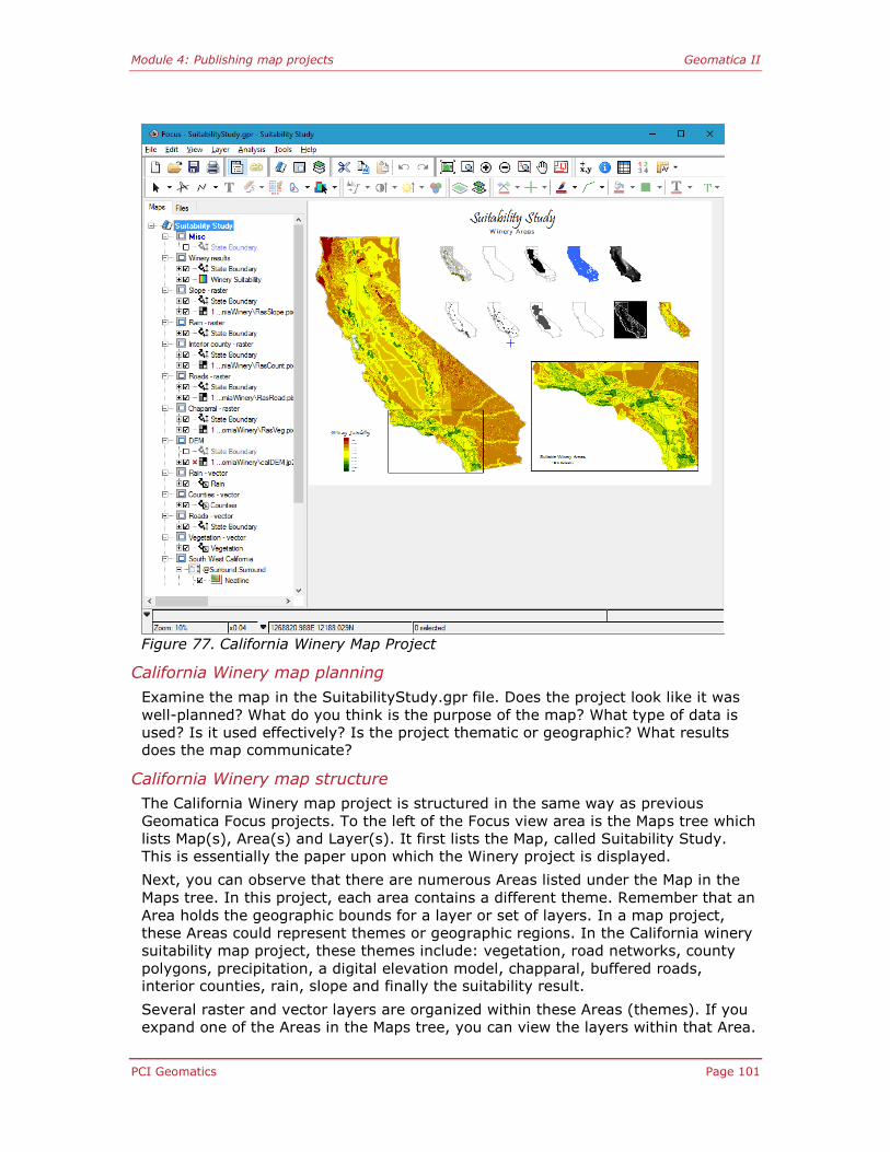
Module 4: Publishing map projects Geomatica II
PCI Geomatics Page 101
Figure 77. California Winery Map Project
California Winery map planning
Examine the map in the SuitabilityStudy.gpr file. Does the project look like it was
well-planned? What do you think is the purpose of the map? What type of data is
used? Is it used effectively? Is the project thematic or geographic? What results does the map communicate?
California Winery map structure
The California Winery map project is structured in the same way as previous
Geomatica Focus projects. To the left of the Focus view area is the Maps tree which
lists Map(s), Area(s) and Layer(s). It first lists the Map, called Suitability Study.
This is essentially the paper upon which the Winery project is displayed.
Next, you can observe that there are numerous Areas listed under the Map in the
Maps tree. In this project, each area contains a different theme. Remember that an
Area holds the geographic bounds for a layer or set of layers. In a map project,
these Areas could represent themes or geographic regions. In the California winery
suitability map project, these themes include: vegetation, road networks, county
polygons, precipitation, a digital elevation model, chapparal, buffered roads, interior counties, rain, slope and finally the suitability result.
Several raster and vector layers are organized within these Areas (themes). If you
expand one of the Areas in the Maps tree, you can view the layers within that Area.

Module 4: Publishing map projects Geomatica II
Page 102 PCI Geomatics
Figure 80. Suitability Study Maps tree
All layers listed in the Maps tree and displayed in the viewer, stem from the Files
tree. The Files tree lists all of the original data files stored on disk. In the Suitability
Study GPR, the original files consist of calDEM.jp2, californ.pix, RasCount.pix,
RasRain.pix, RasRoad.pix, RasSlope.pix, RasVeg.pix, SuitabilityStudy.pix, and
Winery.pix.
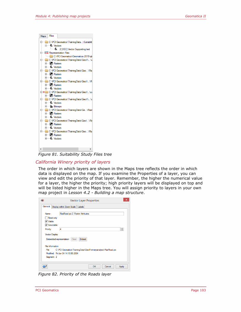
Module 4: Publishing map projects Geomatica II
PCI Geomatics Page 103
Figure 81. Suitability Study Files tree
California Winery priority of layers
The order in which layers are shown in the Maps tree reflects the order in which
data is displayed on the map. If you examine the Properties of a layer, you can
view and edit the priority of that layer. Remember, the higher the numerical value
for a layer, the higher the priority; high priority layers will be displayed on top and
will be listed higher in the Maps tree. You will assign priority to layers in your own map project in Lesson 4.2 - Building a map structure.
Figure 82. Priority of the Roads layer

Module 4: Publishing map projects Geomatica II
Page 104 PCI Geomatics
California Winery representation
Most features in the Suitability Study map project are represented differently than
in the original data layers. For example, the Roads layer was represented with
simple lines before representing different types of roads with various colors and
styles. Most of the map layers need to be represented in a way that communicates
information more effectively than the original data. Geomatica Focus does this using the Representation Editor.
Figure 83. Representation Editor
The Representation Editor is the starting point for creating, assigning, managing
and manipulating the representation of shapes. You will create your own representations in Lesson 4.3 - Representing vector data.
California Winery surround elements
The last map publishing concept is working with surround elements. As mentioned
earlier, surround elements provide context in which to view the map that has been created. Surround elements are stored within individual Areas in a map project.
The surround elements in the Suitability Study map project include items like title,
legend, and neatline. These surround elements are also listed in the Maps tree. In
Geomatica Focus you can create and edit surround elements from the Maps tree.
You will create surround elements for your own map project in Lesson 4.4 -
Building a map surround.

Module 4: Publishing map projects Geomatica II
PCI Geomatics Page 105
Figure 78. Suitability Study Surround Elements
Lesson summary
In this lesson you:
Explored a completed map project file
Learned the concepts of:
map planning
map structure
priority of layers
representation
surround elements
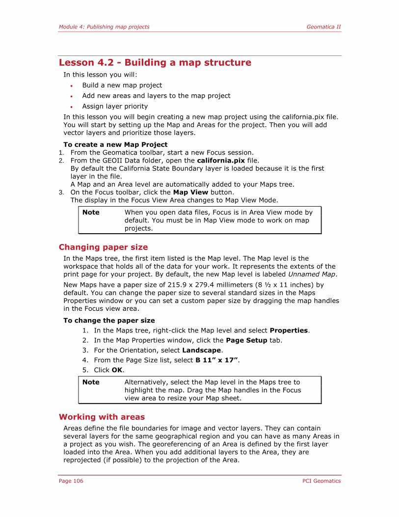
Module 4: Publishing map projects Geomatica II
Page 106 PCI Geomatics
Lesson 4.2 - Building a map structure
In this lesson you will:
Build a new map project
Add new areas and layers to the map project
Assign layer priority
In this lesson you will begin creating a new map project using the california.pix file.
You will start by setting up the Map and Areas for the project. Then you will add vector layers and prioritize those layers.
To create a new Map Project
1. From the Geomatica toolbar, start a new Focus session.
2. From the GEOII Data folder, open the california.pix file.
By default the California State Boundary layer is loaded because it is the first
layer in the file.
A Map and an Area level are automatically added to your Maps tree.
3. On the Focus toolbar, click the Map View button.
The display in the Focus View Area changes to Map View Mode.
Note When you open data files, Focus is in Area View mode by
default. You must be in Map View mode to work on map
projects.
Changing paper size
In the Maps tree, the first item listed is the Map level. The Map level is the
workspace that holds all of the data for your work. It represents the extents of the print page for your project. By default, the new Map level is labeled Unnamed Map.
New Maps have a paper size of 215.9 x 279.4 millimeters (8 ½ x 11 inches) by
default. You can change the paper size to several standard sizes in the Maps
Properties window or you can set a custom paper size by dragging the map handles in the Focus view area.
To change the paper size
1. In the Maps tree, right-click the Map level and select Properties.
2. In the Map Properties window, click the Page Setup tab.
3. For the Orientation, select Landscape.
4. From the Page Size list, select B 11” x 17”.
5. Click OK.
Note Alternatively, select the Map level in the Maps tree to
highlight the map. Drag the Map handles in the Focus
view area to resize your Map sheet.
Working with areas
Areas define the file boundaries for image and vector layers. They can contain
several layers for the same geographical region and you can have as many Areas in
a project as you wish. The georeferencing of an Area is defined by the first layer
loaded into the Area. When you add additional layers to the Area, they are
reprojected (if possible) to the projection of the Area.

Module 4: Publishing map projects Geomatica II
PCI Geomatics Page 107
You can add new Areas to a Map and place layers within the Areas. Layers can hold
raster or vector data such as polygons, points, and segments to be displayed on
your map. Surrounds and indices are associated with Areas, but you work with these elements independently.
You can adjust the bounds of an Area independently from a Map. When you add an
Area, it is listed below the Map in the Maps tree. Vector and raster layers contained
within the Area are listed below the Area. If you resize or move an Area so that
part of it lies outside the extents of the Map (paper), the Area appears red in the
Maps tree.
In this lesson you will create a new map project with two Areas. The Areas will be
of the same geographic region (California), but will display different themes of
information. One Area will display the information about the natural environment and the other Area will display the information about the built environment.
Next, you will rename your first Area level.
To rename your first Area
1. In the Maps tree, click the New Area level.
The Area level is highlighted.
2. Click the New Area level again.
You can now enter a name for your Area.
3. Type Natural.
You now have one Area associated with your Map named Natural that contains the
State Boundary layer. You will now create a second Area to contain data associated with the Built environment.
To create another Area
In the Maps tree, right-click the Map level and select New Area. A New Area is added to the Maps tree beneath the Map level.
The New Area is automatically scaled to the best fit for the dimensions of the Map.
At the moment, the new Area contains no raster or vector data. When you add new
data to this area, Focus automatically scales it the scale of the Area.
To name the second Area
1. In the Maps tree, click the New Area level.
The second Area level is highlighted.
2. Click the New Area level again.
You can now enter a name for your Area.
3. Type Built.
You now have two Areas associated with your Map: Natural, and Built. Next you will add the State Boundary layer to the Built Area as well.
To add data to the Built Area
1. In the Maps tree, select the Built area.
Your data will be loaded into the Built area.
2. Click the Files tree.
3. Expand the Vector layer list.
4. Right-click the State Boundary layer and click View.
The State Boundary layer is loaded into the Built area.

Module 4: Publishing map projects Geomatica II
Page 108 PCI Geomatics
When Focus is in Map View mode, you can click an Area in the Maps tree and drag one of the eight handles to manually resize the extents of the Area.
Note The middle handles are used to crop, while the corner
handles are used to rescale.
You can also enter a specific scale for your Area. You will now change the scale of the two Areas and reposition them on your map.
To change the scale of an Area
1. In the Maps tree, right-click the Natural area and select Properties.
2. Under the General tab, enter a Scale of 1:8000000.
3. Click OK.
The scale of the Natural Area changes in the view area.
4. Repeat steps 1 to 4 for the Built area.
Both Areas are now displayed at the same scale.
Now you will position both Areas in the view area leaving enough space to add
surround elements.
To position an Area
1. In the Maps tree, select the Natural Area.
2. In the Focus view area, position your mouse on the outline of the Area
until you see a four-directional arrow.
3. Click and drag the Area to a new position.
4. Repeat steps 1 to 3 for the Built Area.
Note You can also change the Area position under the Layout
tab in the Area Properties window.
Your layout should look similar to the figure below.

Module 4: Publishing map projects Geomatica II
PCI Geomatics Page 109
Figure 79. Setting up Areas in a map project
At this point, you have created a new map project, defined the map (blank sheet),
and added, scaled and positioned two new Areas. The Areas have the same geographic coordinates; however, they will display different information.
Vector layers
Once the areas of your project have been set up, you can add vector layers to the
project to continue adding information to your map. You will work with the
surround elements later, but first you will add vector layers to your project.
In this lesson you will add three vector layers to each Area. The Natural area will
contain vegetation, river and lake layers. The Built area will contain urban, railroad and road layers.
To add vector layers to your project
1. In the Maps tree, select the Natural area.
2. Click the Files tree.
3. Hold down the CTRL key and select the Rivers, Lakes and Vegetation
vector layers.
The three vector layers are highlighted.

Module 4: Publishing map projects Geomatica II
Page 110 PCI Geomatics
4. Right-click one of the three selected vector layers and select View.
The Rivers, Lakes and Vegetation vector layers open within the Natural
area.
5. Repeat steps 1 through 5 to add Roads, Railroads and Urban vector
layers to the Built area.
Figure 86. Natural and Built Areas
After all the layers are added to your project, it may be necessary to assign priority to layers. Layer priority can cause one layer to mask another in the view area.
To change layer priority
1. In the Maps tree, right-click the State Boundary layer in the Built Area
and select Properties.
The Vector Layer Properties window opens.

Module 4: Publishing map projects Geomatica II
PCI Geomatics Page 111
Figure 87. Vector Layer Properties window
Notice that the State Boundary layer has a Priority of 0. Layers with
higher priority levels (larger numbers) mask overlapping layers with lower
priorities.
2. In the Priority box, type 4.
3. Click OK.
The priority for the State Boundary layer is now 4, meaning the layer has
higher priority and is displayed on the top.
Note You can also change the priority of a layer by dragging it
up or down in the Maps tree. Dragging a layer up the tree
list increases its priority. Dragging a layer down the tree
list decreases its priority toward 0.
Lesson summary
In this lesson you:
Built a new map project
Added new areas and layers to the map project
Assigned layer priority

Module 4: Publishing map projects Geomatica II
Page 112 PCI Geomatics
Lesson 4.3 - Representing vector data
In this lesson you will:
Display data using Representation Styles Tables
Edit representation styles
Label shapes
Understanding representation
Representation determines the appearance of shapes. Focus applies a default
representation to shapes on a vector layer that is not linked to a Representation
Style Table (RST). An RST is a look-up table (LUT) that contains a key and the style
associated to that key. The key or the style can also be referred to as a REPCode.
The key links the style in the RST to the shape on the layer. Each layer can link to
only one RST, but you can link an RST to many layers. You can continue using the default, create a new RST, or import an existing RST.
Keys can be added as attributes for shapes, such as in the REPCode field, or you
can use an existing attribute as the key. When an RST is linked to a layer, Focus
identifies the attributes used as keys in the layer and searches for the
corresponding keys in the RST. When a match is found, the associated style is applied to the shape in the layer.
For example, you can associate an RST to the attributes in a field called roadtype.
In the roadtype field, you have a variety of road types such as interstates,
highways, and streets. In the RST, the key is the road type with which you have
styles associated. When a layer is linked to the RST, the shapes are assigned the style according to their key.
A style is composed of one or more parts. Each part has a primitive with a priority.
Primitives are the building blocks of the style. Each primitive is based on a point,
line, or polygon pattern that is designed according to a number of parameters, such
as color. The priority determines which part is placed in front of the other parts in
the style. You can control the order by assigning the part a priority number. Parts with a higher number appear in front of parts with lower numbered priority.
Types of representation style tables
Focus uses three types of RSTs: Default, Direct, and Indirect.
Default RST: Is controlled by Focus and is applied to vector layers in the absence
of any other RST.
Direct RSTs: Is also called Embedded Representation, because the style is
contained in a layer itself. You can create a Direct RST when you change the
appearance of the shapes directly in the view area using tools on the Display
toolbar. Direct RSTs are only available for .pix vector layers.
When you change the appearance of shapes in the view area, Focus creates an RST using the ShapeIDs as the keys. The Direct RST is saved directly in a .pix file.
Indirect RST: Is a separate file (.rst) that contains an RST. You can link an
Indirect RST to one or more layers. You can also convert an Indirect RST into a
Direct RST by embedding it in the layer through its Properties window.
You can build an Indirect RST as System-linked or User-linked.

Module 4: Publishing map projects Geomatica II
PCI Geomatics Page 113
System-linked RST: Is based on an attribute in a layer. To generate the RST,
select an attribute from the layer to become the key; Focus creates styles for each
key based on the style that you design. Focus automatically links the System-linked RST through the key.
User-linked RST: Often called a master RST, is built independently from a layer.
To build the RST, you define the keys and manually create styles associated to the
keys. Once you build the RST, you link the layers to the RST. The keys in the RST
can match an existing attribute in the layer or you can add the keys in a field in the
layer.
You will begin by opening the Attribute Manager for the Vegetation layer and
examining the existing attributes to use for representation.
To view attributes for Representation
In the Maps tree, right-click the Vegetation layer and select Attribute
Manager. The Attribute Manager for the Vegetation layer opens.
Figure 88. Attribute Table for the Vegetation Layer
Notice the VegType attribute. Each shape is categorized based on different
vegetation types. In the Representation Editor you will create styles that link to the
Vegetation layer using the VecType attribute as the key. You will now create different styles for representing the different vegetation types.
To represent data using the Representation Editor
1. In the Maps tree, right-click the Vegetation layer and select
Representation Editor.
The Representation Editor window opens for the Vegetation Layer.
2. If necessary, click More.
This expands the window to access more options.

Module 4: Publishing map projects Geomatica II
Page 114 PCI Geomatics
Figure 89. Representation Editor for the Vegetation Layer
3. From the Attribute list, select VegType.
This will link the representation styles to the VegType attribute in the
Vegetation layer.
4. Make sure the Generate New Styles option is selected.
5. From the Based On list, select More.
The Style Selector window opens.
6. In the Style Selector window, click the Polygon tab.
Various polygon styles are displayed.

Module 4: Publishing map projects Geomatica II
PCI Geomatics Page 115
Figure 90. Style Selector window
7. In the gallery of styles, select the Red Fill polygon style.
8. Click OK.
9. Make sure the Vary color option is enabled and choose a color scheme.
10. Click Update Styles.
Each value has been assigned a solid polygon based on the color scheme
you selected.

Module 4: Publishing map projects Geomatica II
Page 116 PCI Geomatics
Figure 91. Completed Representation Editor for Vegetation
11. Click Apply.
A warning message opens asking if you want to clear all of the direct
(embedded) representation for this layer.
12. Click Yes.
The default representation is cleared and is replaced with new
representation styles.
The RST is now linked to the Vegetation layer. In the Maps tree, the vector layer
symbol for the Vegetation layer has changed from black to blue. The result of your
vegetation representation should look similar to the figure below.
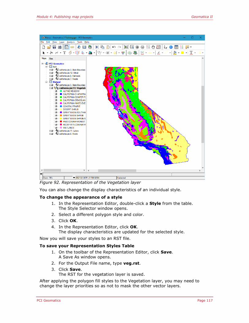
Module 4: Publishing map projects Geomatica II
PCI Geomatics Page 117
Figure 92. Representation of the Vegetation layer
You can also change the display characteristics of an individual style.
To change the appearance of a style
1. In the Representation Editor, double-click a Style from the table.
The Style Selector window opens.
2. Select a different polygon style and color.
3. Click OK.
4. In the Representation Editor, click OK.
The display characteristics are updated for the selected style.
Now you will save your styles to an RST file.
To save your Representation Styles Table
1. On the toolbar of the Representation Editor, click Save.
A Save As window opens.
2. For the Output File name, type veg.rst.
3. Click Save.
The RST for the vegetation layer is saved.
After applying the polygon fill styles to the Vegetation layer, you may need to
change the layer priorities so as not to mask the other vector layers.
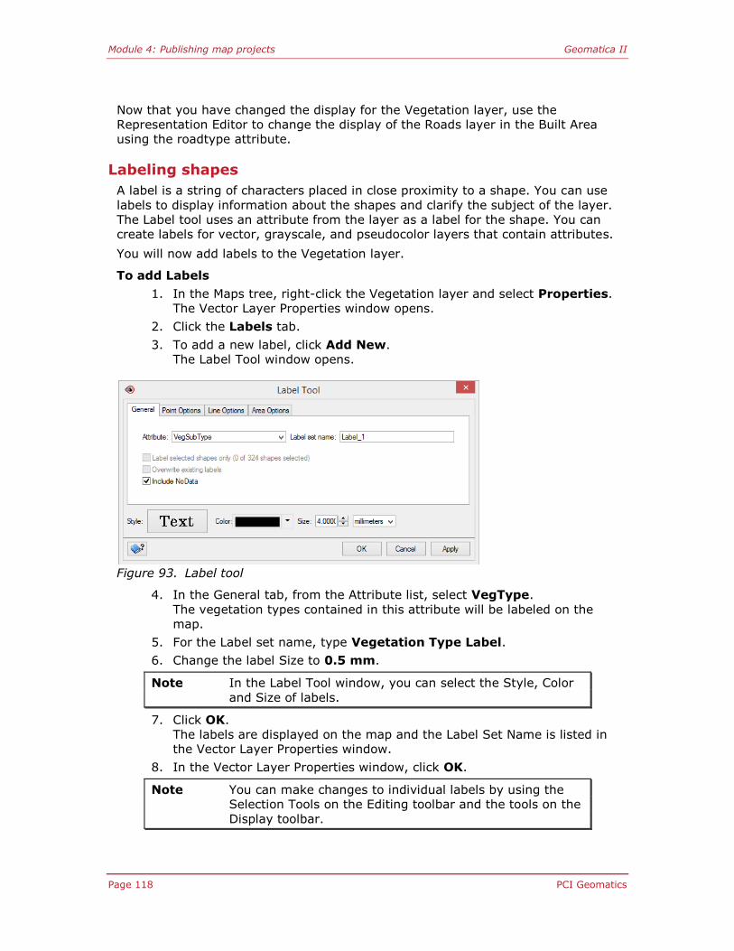
Module 4: Publishing map projects Geomatica II
Page 118 PCI Geomatics
Now that you have changed the display for the Vegetation layer, use the
Representation Editor to change the display of the Roads layer in the Built Area
using the roadtype attribute.
Labeling shapes
A label is a string of characters placed in close proximity to a shape. You can use
labels to display information about the shapes and clarify the subject of the layer.
The Label tool uses an attribute from the layer as a label for the shape. You can
create labels for vector, grayscale, and pseudocolor layers that contain attributes.
You will now add labels to the Vegetation layer.
To add Labels
1. In the Maps tree, right-click the Vegetation layer and select Properties.
The Vector Layer Properties window opens.
2. Click the Labels tab.
3. To add a new label, click Add New.
The Label Tool window opens.
Figure 93. Label tool
4. In the General tab, from the Attribute list, select VegType.
The vegetation types contained in this attribute will be labeled on the
map.
5. For the Label set name, type Vegetation Type Label.
6. Change the label Size to 0.5 mm.
Note In the Label Tool window, you can select the Style, Color
and Size of labels.
7. Click OK.
The labels are displayed on the map and the Label Set Name is listed in
the Vector Layer Properties window.
8. In the Vector Layer Properties window, click OK.
Note You can make changes to individual labels by using the
Selection Tools on the Editing toolbar and the tools on the
Display toolbar.

Module 4: Publishing map projects Geomatica II
PCI Geomatics Page 119
To save your map project
1. On the Focus File menu, click Save Project.
A File To Save window opens.
2. In the File name text box, type CaliEnvironments.gpr.
3. Click Save.
Your project is now saved.
Lesson summary
In this lesson you:
Represented data using the Representation Editor
Edited representation styles
Labeled shapes

Module 4: Publishing map projects Geomatica II
Page 120 PCI Geomatics
Lesson 4.4 - Building a map surround
In this lesson you will:
Add surround elements to your map
Edit properties of surround elements
Surround Elements
A surround is a collection of graphical elements that gives meaning or clarifies the
meaning of geographical information displayed in a Map. It puts the data into context that can be analyzed, organized, and communicated effectively.
The following surround elements are provided in Focus: neatline, border, grid,
legend, picture, north arrow, scale bar, title and paragraph.
Adding surround elements to an area
Surround elements are positioned relative to the neatline of the Area. If an Area
does not contain a neatline, the positioning is based on the Area extents. The
surround elements are displayed in the Maps tree for the Area to which they are
associated. If you place a surround element so that part of it lies outside the boundaries of the Map, it appears red in the Maps tree.
You will begin by adding surround elements to the map. You will then set various
properties for the surround elements.
To create a Surround
1. In the Maps tree, right-click the Natural Area and select Surround.
The Surround window opens.
Figure 94. Surround window

Module 4: Publishing map projects Geomatica II
PCI Geomatics Page 121
2. In the Surround window, click the box next to each surround element.
A check mark appears beside each surround element.
3. Choose a style for a selected element from the Select a QuickStyle list.
Quick Styles are a set of properties that determine the look of a surround
element.
4. Click OK.
The surround elements for the Natural area are added to the Focus view
area and are listed in the Maps tree.
5. Repeat steps 1 to 4 to add surround elements to the Built Area.
The surround elements you selected for the Built area are added to the
Focus view area and are listed in the Maps tree.
Any surround element, except for the neatline, can appear more than once in an
Area. For example, if you want to show two different scales in your map, such as one in kilometers and the other in miles, you can create two scale bars.
You can change the look and position of a surround element through the Properties
window.
To open the Properties window
From the Maps tree, right-click a surround element and click Properties.
Alternatively, double-click the surround element in the Maps tree. The Properties window opens for the selected surround element.
Note Several surround elements contain text that can be
formatted by clicking the Style button in the Properties
window.
You will now edit your surround elements to make a more appropriate grid for your
area.
To edit the Grid spacing
1. From the Maps tree, right-click the Grid surround element and click
Properties.
2. In the Spacing section, select Km for the unit.
3. For the Column width, enter 100.
4. For the Row height, enter100.
Note If you want to keep the number of columns and rows the
same, enable the Keep Equal check box.
5. Click OK.
The Grid updates based on the spacing you entered.
Creating a custom quick style
As you set the properties for surround elements, you build a Current Working Style.
You can save the settings for a surround element in a Quick Style.
When you select a Quick Style, the settings are copied to the Current Working Style
and are applied to the surround item. If you change the properties, the changes are applied to the Current Working Style, not to the Quick Style.
To add a Quick Style to a list
1. From the Maps tree, right-click a surround element and click Properties.
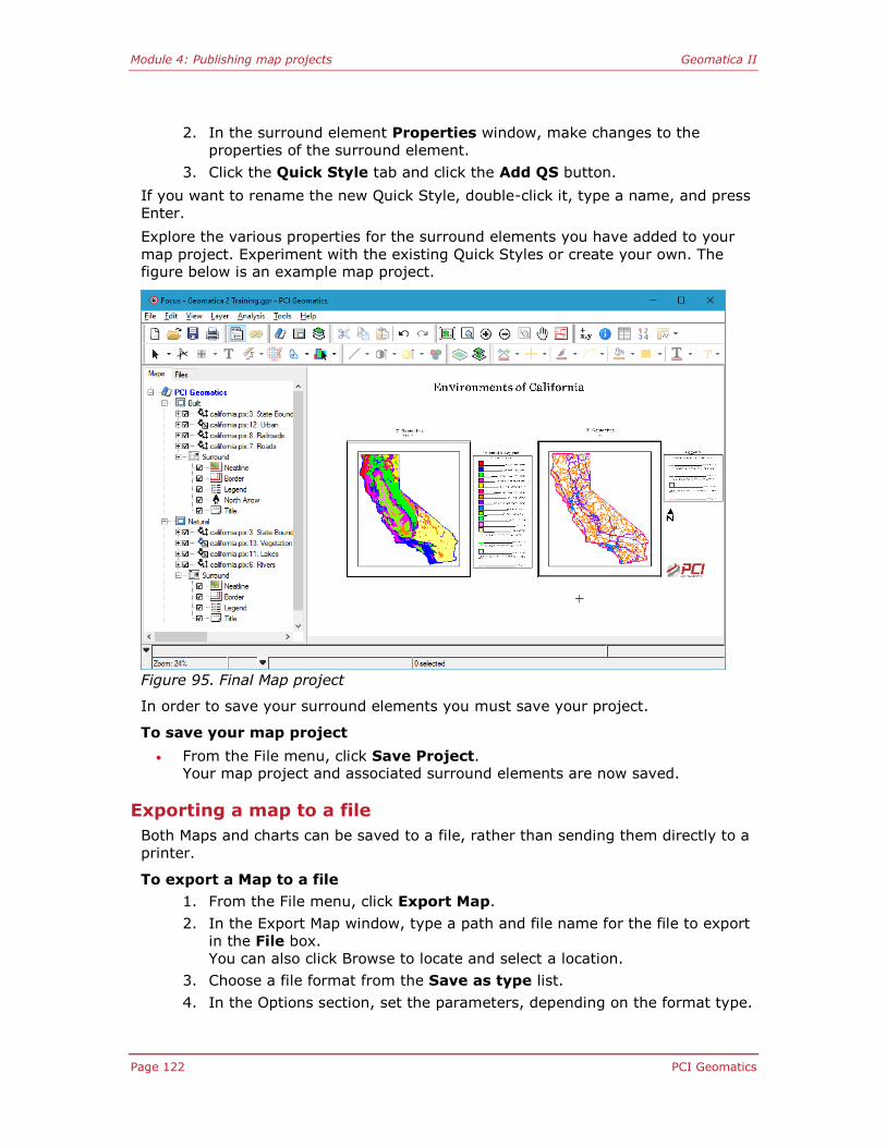
Module 4: Publishing map projects Geomatica II
Page 122 PCI Geomatics
2. In the surround element Properties window, make changes to the
properties of the surround element.
3. Click the Quick Style tab and click the Add QS button.
If you want to rename the new Quick Style, double-click it, type a name, and press
Enter.
Explore the various properties for the surround elements you have added to your
map project. Experiment with the existing Quick Styles or create your own. The figure below is an example map project.
Figure 95. Final Map project
In order to save your surround elements you must save your project.
To save your map project
From the File menu, click Save Project. Your map project and associated surround elements are now saved.
Exporting a map to a file
Both Maps and charts can be saved to a file, rather than sending them directly to a
printer.
To export a Map to a file
1. From the File menu, click Export Map.
2. In the Export Map window, type a path and file name for the file to export
in the File box.
You can also click Browse to locate and select a location.
3. Choose a file format from the Save as type list.
4. In the Options section, set the parameters, depending on the format type.

Module 4: Publishing map projects Geomatica II
PCI Geomatics Page 123
Lesson summary
In this lesson you:
Added surround elements to your map
Edited properties of surround elements

Module 5: Working with Modeler Geomatica II
Page 124 PCI Geomatics
Module 5: Working with Modeler
About this module
Module 5 has three lessons:
Lesson 5.1 - Building a model to convert raster to vector
Lesson 5.2 - Subsetting in Modeler
Lesson 5.3 - Batch processing in Modeler
Modeler
Geomatica Modeler provides an interactive methodology for the development of
both simple and complex data processing flows. Modeler provides access to a
number of standard operations such as data import and export, as well as most EASI/PACE processing algorithms.
You build processing models by placing modules on the Modeler canvas and then
connecting the modules with pipes to create a process flow. You first configure the
modules and then execute the model in either single execution mode or batch
mode. During the execution of the model, graphical cues indicate the data flow
through the process. The Module Librarian enables quick access to all modules.

Module 5: Working with Modeler Geomatica II
PCI Geomatics Page 125
Lesson 5.1 - Building a model to convert raster to vector
In this lesson you will:
Add modules to the Modeler canvas
Connect modules with pipes
Configure various modules
Convert a raster layer to a vector layer
There are many ways to make your imagery more useful and easier to interpret
with PCI Modeler. After classifying an image, you can create vector polygons to
group adjoining pixels that were assigned to a feature or a class during the
classification.
Creating polygons for classified imagery requires some preprocessing. Before
creating your polygons, you will need to create a thematic raster layer with an
attribute table for the raster data. Then, you will use the RAS2POLY module to
convert the thematic raster layer to a polygon layer and then smooth the resulting
vectors using SMMCMASTER. The last stage of your model demonstrates how the
PCI GeoGateway technology in Modeler lets you save your output in a different file format. You will configure an export module to save your output as a SHP file.
The model for this lesson uses a total of six modules from the Module Librarian.
First, you will add an IMPORT module to the Modeler canvas. This IMPORT module inputs the classified image data into your model.
To start Modeler
On the Geomatica toolbar, click the Modeler icon.
Figure 96. Geomatica toolbar Modeler command
The Module Librarian and the Modeler window open on your desktop.
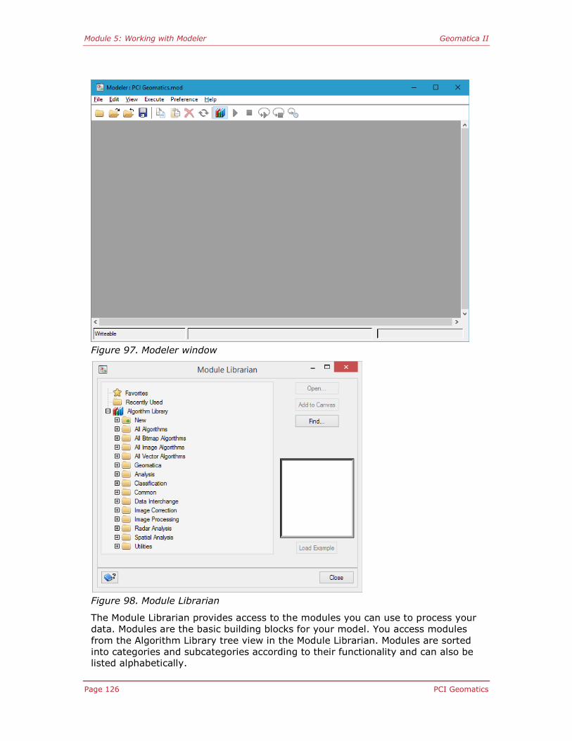
Module 5: Working with Modeler Geomatica II
Page 126 PCI Geomatics
Figure 97. Modeler window
Figure 98. Module Librarian
The Module Librarian provides access to the modules you can use to process your
data. Modules are the basic building blocks for your model. You access modules
from the Algorithm Library tree view in the Module Librarian. Modules are sorted
into categories and subcategories according to their functionality and can also be listed alphabetically.
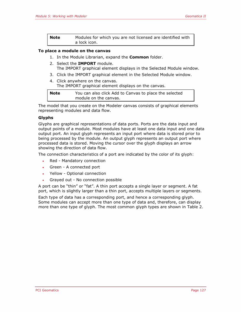
Module 5: Working with Modeler Geomatica II
PCI Geomatics Page 127
Note Modules for which you are not licensed are identified with
a lock icon.
To place a module on the canvas
1. In the Module Librarian, expand the Common folder.
2. Select the IMPORT module.
The IMPORT graphical element displays in the Selected Module window.
3. Click the IMPORT graphical element in the Selected Module window.
4. Click anywhere on the canvas.
The IMPORT graphical element displays on the canvas.
Note You can also click Add to Canvas to place the selected
module on the canvas.
The model that you create on the Modeler canvas consists of graphical elements
representing modules and data flow.
Glyphs
Glyphs are graphical representations of data ports. Ports are the data input and
output points of a module. Most modules have at least one data input and one data
output port. An input glyph represents an input port where data is stored prior to
being processed by the module. An output glyph represents an output port where
processed data is stored. Moving the cursor over the glyph displays an arrow showing the direction of data flow.
The connection characteristics of a port are indicated by the color of its glyph:
Red - Mandatory connection
Green - A connected port
Yellow - Optional connection
Grayed out - No connection possible
A port can be “thin” or “fat”. A thin port accepts a single layer or segment. A fat
port, which is slightly larger than a thin port, accepts multiple layers or segments.
Each type of data has a corresponding port, and hence a corresponding glyph.
Some modules can accept more than one type of data and, therefore, can display more than one type of glyph. The most common glyph types are shown in Table 2.

Module 5: Working with Modeler Geomatica II
Page 128 PCI Geomatics
Table 2. Common Glyphs
Glyph Name
Raster
Lookup Table (LUT)
Bitmap
Vector
Text
Mixed
Georeferencing
Signature
Pseudocolor Table
Ground Control Point
Any
Binary
Math Model
Orbit
Status indicator bar
The color of a module’s status indicator bar indicates the processing mode:
Red - Module is not connected or is improperly configured and will not
execute
Green - Module is properly configured and is ready to execute
Blue - Module is in processing mode
Gray - Processing is complete and data is stored in the cache
Yellow - A warning message has been logged
Now that you have added the IMPORT module to your model, you will select the
input file and layer.
To configure the IMPORT module
1. Double-click the IMPORT module.
The IMPORT Module Control Panel opens.

Module 5: Working with Modeler Geomatica II
PCI Geomatics Page 129
2. On the Input Params 1 tab, click Browse. The File Selector window opens.
3. Locate the GEO Data folder and select irvine.pix.
4. Click Open.
The Available Layers from this file are listed.
5. From the Available Layers list, select 6 [8U] USGS Land Use/Land
Cover.
Figure 99. IMPORT Module Control Panel
6. Click Accept.
The output raster port glyph displays on the IMPORT module and the status indicator bar turns green.
To place the remaining modules on the canvas
1. In the Module Librarian, expand the Spatial Analysis category, then expand the Conversion Tools subcategory and select RAS2THMR.
2. Click the RAS2THRM module in the Selected Algorithm window and click
the canvas to the right of the IMPORT module. Alternatively, right-click
the module listed in the Module Librarian Add to Canvas Click on the
canvas.
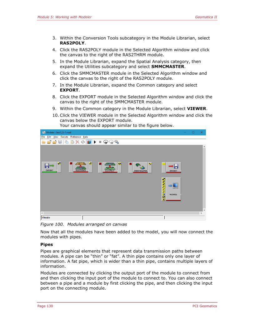
Module 5: Working with Modeler Geomatica II
Page 130 PCI Geomatics
3. Within the Conversion Tools subcategory in the Module Librarian, select RAS2POLY.
4. Click the RAS2POLY module in the Selected Algorithm window and click
the canvas to the right of the RAS2THRM module.
5. In the Module Librarian, expand the Spatial Analysis category, then
expand the Utilities subcategory and select SMMCMASTER.
6. Click the SMMCMASTER module in the Selected Algorithm window and
click the canvas to the right of the RAS2POLY module.
7. In the Module Librarian, expand the Common category and select
EXPORT.
8. Click the EXPORT module in the Selected Algorithm window and click the
canvas to the right of the SMMCMASTER module.
9. Within the Common category in the Module Librarian, select VIEWER.
10. Click the VIEWER module in the Selected Algorithm window and click the
canvas below the EXPORT module.
Your canvas should appear similar to the figure below.
Figure 100. Modules arranged on canvas
Now that all the modules have been added to the model, you will now connect the
modules with pipes.
Pipes
Pipes are graphical elements that represent data transmission paths between
modules. A pipe can be “thin” or “fat”. A thin pipe contains only one layer of
information. A fat pipe, which is wider than a thin pipe, contains multiple layers of information.
Modules are connected by clicking the output port of the module to connect from
and then clicking the input port of the module to connect to. You can also connect
between a pipe and a module by first clicking the pipe, and then clicking the input port on the connecting module.

Module 5: Working with Modeler Geomatica II
PCI Geomatics Page 131
A pipe is default color-coded according to the type of data that it transmits. Some examples are listed in Table 3.

Module 5: Working with Modeler Geomatica II
Page 132 PCI Geomatics
Table 3. Pipe Colors and Data Types
Pipe color Data type
Green Rasters
White Vectors
Red Bitmaps
Blue Pseudocolor tables
Yellow Lookup tables
Cyan Binary
Black Dead pipe
Note The most frequent causes for dead pipes are moving,
renaming, and deleting an input file or layer.
Always connect modules before you configure them, because for some
modules the default settings of an input layer can override a module’s
configuration. An exception is the IMPORT module, which you must configure for it to display a port.
To connect modules
1. Click the output raster port on the IMPORT module and then click the
input raster port on the RAS2THMR module.
A green pipe connects these two modules.
2. Click the output raster port on the RAS2THMR module and then click the
input raster port on the RAS2POLY module.
3. Click the output vector port on the RAS2POLY module and then click the
input port on the SMMCMASTER module.
A white pipe representing vector data connects these two modules.
4. Click the output vector port on the SMMCMASTER module and then click
the input port on the EXPORT module.
To connect a module from a pipe
1. Click the white pipe between the SMMCMASTER and the EXPORT modules.
The pipe displays with a blue border.
2. Click the input vector port on the VIEWER module.
A pipe branches from the original pipe to the VIEWER module.
Note With this type of connection, the same data is sent to
both modules.

Module 5: Working with Modeler Geomatica II
PCI Geomatics Page 133
Figure 101. Modules connected with pipes
Sometimes the orientation of a module can make it awkward to connect to another
module. By rotating a module, all ports on the module rotate which can simplify the display of the pipes.
To rotate a module
1. Click the VIEWER module on the canvas. The module displays with a blue border.
2. On the Modeler toolbar, click the Rotate button.
The module rotates 90 degrees clockwise. You may wish to reposition this module.
Figure 102. Rotated module
To configure the RAS2THMR module

Module 5: Working with Modeler Geomatica II
Page 134 PCI Geomatics
1. Double-click the RAS2THMR module. The RAS2THMR Module Control Panel opens.
Figure 103. RAS2THMR Module Control Panel
2. For the Create Attributes option, select Area Perimeter.
3. Click Accept.
To configure the RAS2POLY module
1. Double-click the RAS2POLY module. The RAS2POLY Module Control Panel opens.
Figure 104. RAS2POLY Module Control Panel

Module 5: Working with Modeler Geomatica II
PCI Geomatics Page 135
2. Ensure the Smooth vectors option is checked.
3. Click Accept.
To configure the SMMCMASTER module
1. Double-click the SMMCMASTER module.
The SMMCMASTER Module Control Panel opens.
Figure 105. SMMCMASTER Module Control Panel
2. For the Tolerance Value, enter 1. The larger the tolerance value, the greater the smoothing.
3. Click Accept.
To configure the EXPORT module
1. Double-click the EXPORT module. The EXPORT Module Control Panel opens.
Figure 106. EXPORT Module Control Panel

Module 5: Working with Modeler Geomatica II
Page 136 PCI Geomatics
2. On the Input Params 1 tab, click Browse. The File Selector window opens.
3. Navigate to the GEO Data folder.
4. In the File name box, type smooth_polygons.shp and click Save.
The file name appears in the Module Control Panel.
5. From the Format list, select ArcView Shapefile (.shp).
6. Click Accept. The EXPORT Module Control Panel closes and is now configured.
You are now ready to execute your model.
To execute a model
From the Execute menu, select Run or click the Run button on the toolbar.
The status indicator bars on the modules show the progress of each operation
as it is executed. Another progress indicator in the display area of the Modeler window monitors the progress of the entire model.
When the model has finished executing, the Modeler Viewer opens and displays the
results. The results are also written to the specified output file.
Figure 107. Results of raster to vector conversion

Module 5: Working with Modeler Geomatica II
PCI Geomatics Page 137
Caches
After a model has executed without errors, bulges (called caches) containing
intermediate files are formed. To save a file stored in a cache, you must attach an Export module to the pipe containing the cache.
To view cache contents
1. Click a cache bulge.
2. Right-click and select View Cache, 1 or 3 Layers.
The layer is displayed in the Cache Viewer. A Cache Viewer displays the
first layer if fewer than three layers are available. If three or more layers
are available, then the first three layers are displayed.
Note You can also view the cache contents by double-clicking
the cache bulge.
Pipe contents and cache contents are the same.
To reduce processing time, do not clear caches after re-
configuring a module or an executed model. When you re-
run the updated model, only the re-configured module
and all modules directly downstream from it will re-run.
Saving a model
Now that you have created your first model with Modeler, you will save the model as a MOD file.
To save your model
1. From the File menu, select Save Model. The File Selector window opens.
2. Navigate to the GEO Data folder.
3. In the File Name box, type raster_to_vector.mod.
4. Click Save.
The File Selector window closes and your model is saved as a MOD file.
Note When you save a model after it has executed, the
intermediate and output files are not saved with the
model.
Lesson summary
In this lesson you:
Added modules to the Modeler canvas
Connected modules with pipes
Configured various modules
Converted a raster layer to a vector layer

Module 5: Working with Modeler Geomatica II
Page 138 PCI Geomatics
Lesson 5.2 - Subsetting in Modeler
In this lesson you will:
Create a subset using CLIP
Create a submodel using RELEASE and ACCUMULATE
Execute the model in Batch mode
CLIP module
A componentized version of the clipping/subsetting functionality available in Focus
is available in Modeler as a CLIP module. The CLIP module allows you to
incorporate clipping into processing models. Batch clipping is also enabled through
this module.
In this example, you will create a subset using the CLIP module. A submodel will
then be added to split the raster layers and filter them using FAV. The results will be exported to a new file.
In addition to the Module Librarian, Modeler provides a shortcut menu in the
Modeler workspace for adding the modules you use most often.
To add your input modules to the canvas
1. Right-click anywhere on the Modeler canvas.
A shortcut menu opens.
2. In the Common Modules submenu, click Import.
The IMPORT module is ready to be placed on the Modeler canvas.
Figure 108. Shortcut menu on the Modeler canvas
Module 5: Working with Modeler Geomatica II
PCI Geomatics Page 139
3. Click the Modeler canvas. The IMPORT module appears on the canvas.
To configure the IMPORT module
1. Double-click the IMPORT module.
The IMPORT Module Control Panel opens.
2. On the Input Params 1 tab, click Browse.
3. Locate the GEO Data folder and select irvine.pix.
4. Click Open.
The Available Layers from this file are listed.
5. From the Available Layers list, select all available layers.
The IMPORT graphical element expands and ports for each of the selected layer types appear.
Note To select all layers of one type, click the check box beside
the layer type category.
TYPESPLIT
This module separates mixed port data types into individual port data types. The
input port for a TYPESPLIT module is always a Mixed input port. You must configure
the TYPESPLIT module to display the required output port or ports. All input layers
that do not fall into any of the selected data types will be output to the mixed output port.
RELEASE
The RELEASE module releases all incoming layers in sequence by layer or by group
during batch execution. Release takes place during each model execution until all groups or layers have been released.
ACCUMULATE
The ACCUMULATE module accumulates all incoming layers during batch execution.
When all possible batch runs have completed and all modules executed, these
accumulated layers will be released at the output port and made available for use
to the subsequent modules. During accumulation, the output port of ACCUMULATE
will be blocked disabling all subsequent modules.
The RELEASE and ACCUMULATE modules can be used to embed a submodel into an
existing model, each with its own number of scheduled batch runs. The submodel
uses the incoming data from the RELEASE module to establish its batch execution
status. The RELEASE module acts as a batch run generator, transforming a set of
incoming layers into a set of batch parameter sets. Once the modules in the
submodel have executed, the batch parameter sets are accumulated and passed
back into the parent model. They allow the execution of the parent model to be suspended until the embedded module has completed its own batch execution.
To place the remaining modules on the canvas
1. From the Spatial Analysis\Utilities folder, select the CLIP module.
2. Add the CLIP module to the Modeler canvas.
3. Right-click the canvas, and choose Common Modules, TypeSplit.
4. Click the canvas.
The TYPESPLIT module displays on the canvas.

Module 5: Working with Modeler Geomatica II
Page 140 PCI Geomatics
5. Repeat steps 3 and 4 to add RELEASE, ACCUMULATE and EXPORT modules to the canvas.
Note You can also access TYPESPLIT, RELEASE and
ACCUMULATE modules from the Common folder in the
Module Librarian.
6. From the Image Processing\Image Filtering folder, select FAV.
7. Arrange your modules similar to figure below.
Figure 109. Modules arranged on canvas
To connect the modules
1. Click the Output Mixed port on the IMPORT module and then click the
Input Mixed port on the CLIP module.
A white pipe connects these two modules.
2. Click the Output Mixed port on the CLIP module and then click the input Mixed Layers port on the TYPESPLIT module.
3. Click the Output Rasters port on the TYPESPLIT module and then click
the Input port on the RELEASE module.
4. Click the Output port on the RELEASE module and then click the input
raster port on the FAV module.
5. Click the output raster port on the FAV module and then click the Input
port on the ACCUMULATE module.
6. Click the Output port on the ACCUMULATE module and then click the
Input Raster port on the EXPORT module.
7. Click the Output Mixed port on the TYPESPLIT module and then click
the Input Mixed port on the EXPORT module.
8. Rotate the modules as necessary.
Your model should look similar to the figure below.

Module 5: Working with Modeler Geomatica II
PCI Geomatics Page 141
Figure 110. Modules connected with pipes
Now that you have places all the necessary modules on the canvas and have connected them with pipes, you will configure them.
To configure the CLIP module
1. Double-click the CLIP module.
The CLIP Module Control Panel opens.
Figure 111. CLIP Module Control Panel
2. For Coordinate Type, choose Raster extents.

Module 5: Working with Modeler Geomatica II
Page 142 PCI Geomatics
3. For the Upper Left coordinate, enter 0,150.
4. For the Lower Right coordinate, enter 256, 406.
5. Click Accept.
To configure the TYPESPLIT module
1. Double-click the TYPESPLIT module.
The TYPESPLIT Module Control Panel opens.
Figure 112. TYPESPLIT Module Control Panel
2. Ensure that the Rasters option is selected.
3. Click Accept.
To configure the RELEASE module
1. Double-click the RELEASE module.
The RELEASE Module Control Panel opens.

Module 5: Working with Modeler Geomatica II
PCI Geomatics Page 143
Figure 113. RELEASE Module Control Panel
2. For the Release Method, select By Layer.
This option will release each individual layer to the output port.
3. Click Accept.
To configure the FAV module
1. Double-click the FAV module. The FAV Module Control Panel opens.
Figure 114. FAV Module Control Panel
2. For the Filter X Size and the Filter Y Size, enter 7.
3. Click Accept.
To configure the EXPORT module
1. Double-click the EXPORT module. The EXPORT Module Control Panel opens.

Module 5: Working with Modeler Geomatica II
Page 144 PCI Geomatics
Figure 115. Export Module Control Panel
2. On the Input Params 1 tab, click Browse. The File Selector window opens.
3. Navigate to the GEO Data folder.
4. In the File name box, type clipped.pix and click Save.
5. Click Accept.
The EXPORT Module Control Panel closes and is now configured.
The RELEASE module has the effect of turning a single run setup into a Batch
setup. In order for all three raster layers to be filtered and exported, the model
needs to be run in batch mode; otherwise, only the first raster layer would be
released to FAV and then passed to EXPORT.
To execute the model
From the Execute menu, select Run Batch or click the Run Batch button on
the toolbar.
The status indicator bars on the modules show the progress of each operation
as it is executed. Another progress indicator in the display area of the Modeler
window monitors the progress of the entire model.
The results are written to the specified output file.
Lesson summary
In this lesson you:
Created a subset using CLIP
Created a submodel using RELEASE and ACCUMULATE
Executed the model in Batch mode

Module 5: Working with Modeler Geomatica II
PCI Geomatics Page 145
Lesson 5.3 - Batch processing in Modeler
In this lesson you will:
Construct a model
Configure the modules for batch processing
Execute the model in Batch mode
Batch processing
Each configurable module has a Batch Parameter Sets table, which is used to
configure a module for batch mode. Batch parameter sets are defined on a
module's control panel and include all parameters that can be configured for one
batch pass.
Generally, when processing in batch mode, Modeler applies the first batch
parameter set (first row of a Batch Parameter Sets table) of the first module.
Modeler then applies the first batch parameter set of the second module, and so on
until the first batch parameter sets of all modules have been executed. The above
process is repeated for each subsequent batch parameter set of each module until
all parameter sets have been executed.
Modeler performs three basic types of batch processing:
one file-to-many batch parameter sets - Modeler processes the same input
file or layer with different batch parameter sets
many files-to-one batch parameter set - Modeler processes each input file or
layer with the same batch parameter set
many files-to-many batch parameter sets - Modeler processes each input file
or layer with a unique batch parameter set
The model you will create in this lesson uses the DEM layers of irvine.pix,
rabbit_lake_dem.pix and toronto_dem.pix as input. Ten meter contours will be
generated from the irvine.pix file, 25 m contours from the rabbit_lake_dem.pix file,
and 50 m contours from the toronto_dem.pix file; each new vector layer will be
saved in a new file and will be displayed in separate viewers. The IMPORT,
CONTOUR, EXPORT and the VIEWER modules will be configured for batch processing.
To place the IMPORT module on the canvas
1. Right-click the canvas, and choose Common Modules, Import.
2. Click the canvas.
The IMPORT module displays on the canvas.
To set the batch parameters for the IMPORT module
1. Double-click the IMPORT module. The IMPORT Module Control Panel opens.
2. On the IMPORT Module Control Panel, click Batch.
The Module Control Panel expands.

Module 5: Working with Modeler Geomatica II
Page 146 PCI Geomatics
Figure 116. Expanded IMPORT Module Control Panel
3. In the Batch Parameter Sets table, right-click the File column heading,
and choose Add Files.
The File Selector window opens.
4. Navigate to the GEO Data folder.
5. Press the CTRL key, and choose irvine.pix and rabbit_lake_dem.pix.
The file names display in the Batch Parameter Sets table.
6. In the Batch Parameter Sets table, choose irvine.pix.
7. On the Input Params 1 tab, from the Available Layers list, enable the
check box for the 10[16S] USGS Elevation Data layer. The Raster column displays in the Batch Parameter Sets table.
8. In the Batch Parameter Sets table, choose rabbit_lake_dem.pix.
9. On the Input Params 1 tab, from the Available Layers list, enable the check box for the 1[16S] DEM layer.
10. Click Accept.

Module 5: Working with Modeler Geomatica II
PCI Geomatics Page 147
To place the remaining modules on the canvas
1. From the Analysis\DEM Analysis folder select, CONTOUR.
2. Add the CONTOUR module to the canvas.
3. Right-click the canvas, and choose Common Modules, Export.
4. Click the canvas to the right of the CONTOUR module.
5. Right-click the canvas, and choose Common Modules, Viewer.
6. Click the canvas below the EXPORT module.
Your canvas should look similar to the figure below.
Figure 117. Modules arranged on the canvas
To connect the modules
1. Click the output raster port on the IMPORT module and then click the
input raster port on the CONTOUR module.
A green pipe displays connecting these two modules.
2. Click the output vector port on the CONTOUR module and then click the
input port on the EXPORT module.
A white pipe connects these two modules.
3. Click the output pipe from the CONTOUR module and then click the Input
Vector port on the VIEWER module.
Now that the model is constructed, you need to set the batch parameters for the CONTOUR module.
To set the batch parameters for the CONTOUR module
1. Double-click the CONTOUR module.
The CONTOUR Module Control Panel opens.
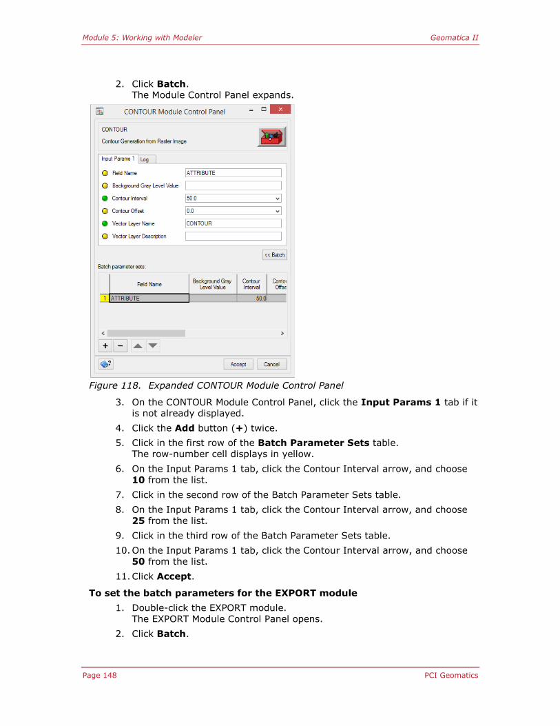
Module 5: Working with Modeler Geomatica II
Page 148 PCI Geomatics
2. Click Batch. The Module Control Panel expands.
Figure 118. Expanded CONTOUR Module Control Panel
3. On the CONTOUR Module Control Panel, click the Input Params 1 tab if it is not already displayed.
4. Click the Add button (+) twice.
5. Click in the first row of the Batch Parameter Sets table.
The row-number cell displays in yellow.
6. On the Input Params 1 tab, click the Contour Interval arrow, and choose
10 from the list.
7. Click in the second row of the Batch Parameter Sets table.
8. On the Input Params 1 tab, click the Contour Interval arrow, and choose
25 from the list.
9. Click in the third row of the Batch Parameter Sets table.
10. On the Input Params 1 tab, click the Contour Interval arrow, and choose
50 from the list.
11. Click Accept.
To set the batch parameters for the EXPORT module
1. Double-click the EXPORT module.
The EXPORT Module Control Panel opens.
2. Click Batch.

Module 5: Working with Modeler Geomatica II
PCI Geomatics Page 149
Figure 119. Expanded EXPORT Module Control Panel
3. In the Batch Parameter Sets table, right-click the File column heading,
and choose From Input Module.
The From Input Module window opens. If your model contains more than
one IMPORT module, you would select from which module to select the
input file names.
4. Click OK.
The Batch Parameter Sets table updates with the names of the input files.
5. Press the SHIFT key, and select all three parameter sets.
6. In the Batch Parameter Sets table, right-click the File column heading,
and choose Add Prefix/Suffix. The Add Prefix/Suffix window opens.
Figure 120. Add Prefix/Suffix window

Module 5: Working with Modeler Geomatica II
Page 150 PCI Geomatics
7. In the Add Prefix/Suffix window, click the Suffix Text check box and enter
_contours.
This option applies to all three selected cells.
8. Click OK.
The File names update in the Batch Parameter Sets table.
9. Click Accept.
To set the batch parameters for the VIEWER module
1. Double-click the VIEWER module. The VIEWER Module Control Panel opens.
2. Click Batch.
Figure 121. VIEWER Module control panel
3. Click the Add button (+) twice.
4. Double-click the first cell of the first row.
The row-number cell displays in yellow, and on the Input Params tab, the Viewer Name box is selected.
5. In the Viewer Name box, type Contour10.
6. Double-click the first cell of the second row.
7. In the Viewer Name box, type Contour25.
8. Double-click the first cell of the third row.
9. In the Viewer Name box, type Contour50.
10. Click Accept.

Module 5: Working with Modeler Geomatica II
PCI Geomatics Page 151
You can configure all modules of a model in batch mode and then run the model in
non-batch mode to check that your model is correctly set up. In this process, the
parameter set displayed on the Input Params 1 tab of a module's control panel or selected in the Batch Parameter Sets table, is applied.
To test the irvine.pix file:
1. Double-click the IMPORT module.
2. Click Batch, and in the Batch Parameter Sets table, choose irvine.pix.
3. Click Accept.
4. Double-click the CONTOUR module.
5. Click Batch, and in the Batch Parameter Sets table, choose the first batch
parameter set.
6. Click Accept.
7. Double-click the EXPORT module.
8. Click Batch, and in the Batch Parameter Sets table, choose the first batch
parameter set.
9. Click Accept.
10. Click the VIEWER module.
11. Click Batch, and in the Batch Parameter Sets table, choose the first batch
parameter set.
12. Click Accept.
13. On the toolbar, click Run.
The Viewer window displays the results of the selected batch parameter
set.
14. Close the Viewer window.
Figure 122. Modules with Pipes connected

Module 5: Working with Modeler Geomatica II
Page 152 PCI Geomatics
To run the model in batch mode
From the Execute menu, choose Run Batch or click the Run Batch button on
the toolbar.
When the run is complete, the Modeler Viewer 10, the Modeler Viewer 25 and
the Modeler Viewer 50 windows open.
Lesson summary
In this lesson you:
Constructed a model
Configured the modules for batch processing
Executed the model in Batch mode

Optional Modules Geomatica II
PCI Geomatics Page 153
Optional Modules
Module 1: Performing atmospheric
correction
About this module Module 2 has two lessons:
Lesson 1.1 - Cloud and haze removal
Lesson 1.2 - Atmospherically correcting imagery to Ground Reflectance
Why atmospheric correction?
Optical satellite sensors are an important source of information for scientific
investigations of the environment. However, haze from water vapor and aerosol
particles influence the recorded signal and mask important ground spectra. In
addition, topographic effects can strongly influence the recorded signal. In rugged
terrain, varying illumination conditions (sunny and shady slopes) modify the true spectral behavior of surfaces.
The objective of an atmospheric/topographic correction is the elimination of
atmospheric and illumination effects to retrieve proper physical parameters of the
earth’s surface (for example, surface reflectance, emissivity, and temperature). It
is an essential part of preprocessing and a prerequisite for derivation of many value-added products.
Improvement for data analysis
There are several ways atmospheric correction of satellite images improves data
analysis:
The influences of atmosphere and solar illumination are removed or greatly reduced.
Multi-temporal scenes recorded under different atmospheric conditions can be
compared more easily after atmospheric correction so that observed changes
are due to changes on the earth's surface and not due to different atmospheric conditions.
Results of change detection and classification algorithms can be improved if
careful consideration of the sensor calibration aspect is taken into account.
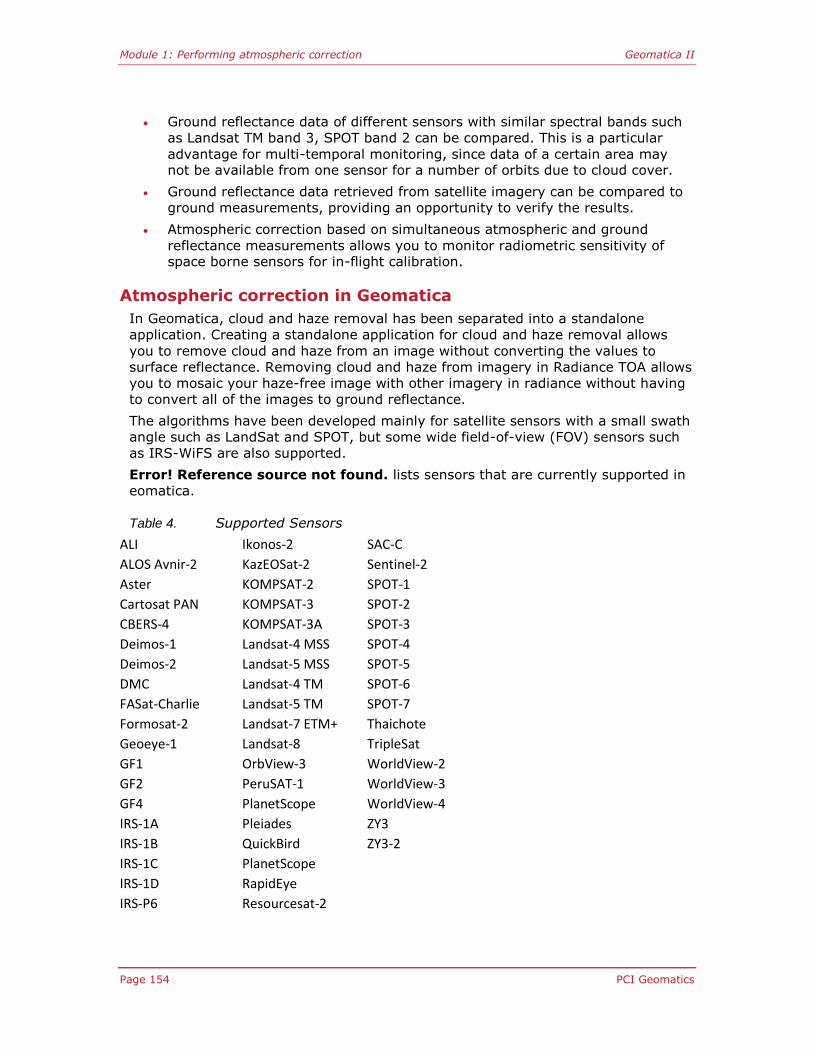
Module 1: Performing atmospheric correction Geomatica II
Page 154 PCI Geomatics
Ground reflectance data of different sensors with similar spectral bands such
as Landsat TM band 3, SPOT band 2 can be compared. This is a particular
advantage for multi-temporal monitoring, since data of a certain area may not be available from one sensor for a number of orbits due to cloud cover.
Ground reflectance data retrieved from satellite imagery can be compared to
ground measurements, providing an opportunity to verify the results.
Atmospheric correction based on simultaneous atmospheric and ground
reflectance measurements allows you to monitor radiometric sensitivity of space borne sensors for in-flight calibration.
Atmospheric correction in Geomatica
In Geomatica, cloud and haze removal has been separated into a standalone
application. Creating a standalone application for cloud and haze removal allows
you to remove cloud and haze from an image without converting the values to
surface reflectance. Removing cloud and haze from imagery in Radiance TOA allows
you to mosaic your haze-free image with other imagery in radiance without having
to convert all of the images to ground reflectance.
The algorithms have been developed mainly for satellite sensors with a small swath
angle such as LandSat and SPOT, but some wide field-of-view (FOV) sensors such
as IRS-WiFS are also supported.
Error! Reference source not found. lists sensors that are currently supported in
eomatica.
Table 4. Supported Sensors
ALI Ikonos-2 SAC-C
ALOS Avnir-2 KazEOSat-2 Sentinel-2
Aster KOMPSAT-2 SPOT-1
Cartosat PAN KOMPSAT-3 SPOT-2
CBERS-4 KOMPSAT-3A SPOT-3
Deimos-1 Landsat-4 MSS SPOT-4
Deimos-2 Landsat-5 MSS SPOT-5
DMC Landsat-4 TM SPOT-6
FASat-Charlie Landsat-5 TM SPOT-7
Formosat-2 Landsat-7 ETM+ Thaichote
Geoeye-1 Landsat-8 TripleSat
GF1 OrbView-3 WorldView-2
GF2 PeruSAT-1 WorldView-3
GF4 PlanetScope WorldView-4
IRS-1A Pleiades ZY3
IRS-1B QuickBird ZY3-2
IRS-1C PlanetScope IRS-1D RapidEye IRS-P6 Resourcesat-2

Module 1: Performing atmospheric correction Geomatica II
PCI Geomatics Page 155
Atmospheric Correction in the Geomatica Focus environment is an interactive
process that can be repeated until a satisfactory result is achieved. You can use
several different input layers including haze and cloud masks, raw data layers,
elevation data, and associated information. Output data includes corrected layers
and visibility layers. You can also use several kinds of value-added layers such as
vegetation and leaf area indices.

Module 1: Performing atmospheric correction Geomatica II
Page 156 PCI Geomatics
Lesson 1.1 – Cloud Masking & Haze Removal
In this lesson you will:
Apply cloud and haze masking techniques on a SPOT-4 data set
Remove haze from a SPOT-4 scene
Cloud and haze masking
In this lesson, you will apply cloud and haze masking techniques to reduce the
impact of cloud and haze in the image. The dataset you will be working with is a
SPOT4 scene in Nova Scotia, Canada. The imagery is provided courtesy of www.GeoBase.ca.
To start a new project
From the Focus File menu, select New Project. All items will be cleared from the Maps and Files trees.
You will now open the Atmospheric Correction window and begin setting up for the
atmospheric correction of a SPOT-4 image.
To select the image file to correct
1. From the Focus menu, select Open to display the File Selector window.
2. Navigate to GeoII Data folder.
3. Select S4_06448_4438_20061008_M20_Raw.pix and
S4_06448_4438_20061008_P10_Raw.pix and click Open.
Figure 123. SPOT4 image illustrating haze1
4. From the Focus menu, select Analysis | Atmospheric Correction |
Haze Removal and Cloud Masking. The Atmospheric Correction window opens.
5. From the Haze Removal workflow, select Sensor and image setting.
6. In the Sensor and image setting panel, select the SPOT4 scene:
1 Image courtesy of geobase.ca.

Module 1: Performing atmospheric correction Geomatica II
PCI Geomatics Page 157
select S4_06448_4438_20061008_M20_Raw.pix as the multispectral file
select S4_06448_4438_20061008_P10_Raw.pix as the panchromatic
file
7. In the Output Files section, select the folder in which you installed the
GeoII training data. For example, C:\PCI Geomatics\Geomatica
2018\GeoII.
Figure 124. Atmospheric Correction window Haze Removal workflow
8. After the information has been validated, click the Next button to proceed to the Haze and cloud masking parameters.
9. Review the Haze and cloud masking parameters.
10. Click the Run button.
When the Haze and cloud masking task is complete, the imagery is
automatically loaded in Focus. You should review the quality of the
results, and analyze the cloud, haze, and water masks.
It is likely that the cloud, haze, and water masks will require some manual
editing. Alternatively, if you do not want to edit the cloud mask, you can
recalculate the cloud mask by adjusting the cloud threshold values. These
values are derived from the Top of Atmosphere reflectance values. If you
prefer to let the system mask the clouds, you must perform TOA
Reflectance, analyze the digital numbers for cloud pixels, and enter the reflectance values for the pixels representing clouds.
11. After editing the masks, select the Radio button Import from file for
both the Cloud mask and Water mask.
12. Select both the Cloud Mask Layer and the Water Mask layer for each
mask
13. Alternatively, if you did not save changes to the cloud or water mask in
step 12 above, then edit the corresponding seed and threshold values.

Module 1: Performing atmospheric correction Geomatica II
Page 158 PCI Geomatics
The NIR band in SPOT-4 has a wavelength range of 0.78 to 0.89
micrometers. It may be necessary to remove effects of haze from the NIR
band.
14. Inspect the NIR band as a grayscale image to see if any haze is visible.
15. If haze is present in the NIR band, set the Apply haze correction to bands
under value to 0.89 micrometers so that haze and cloud removal is
applied to that band.
16. Inspect the SWIR band, and adjust if necessary.
Figure 125. Atmospheric Correction window with updated Haze Removal
parameters
17. Re-run the Haze and cloud removal workflow.
18. Examine the results and, if necessary, adjust the masks or masking
parameters.

Module 1: Performing atmospheric correction Geomatica II
PCI Geomatics Page 159
Figure 95. Results of Haze Removal operation2
Lesson summary
In this lesson you:
Set up for haze removal
Attempted haze removal using default values
Visually inspected the results
Manually adjusted the cloud and haze masks
Ran the Haze and cloud removal workflow with adjusted masks and
parameters
Visually inspected the results
2 Image courtesy of geobase.ca.

Module 1: Performing atmospheric correction Geomatica II
Page 160 PCI Geomatics
Lesson 1.2 - Atmospherically correcting imagery to Ground Reflectance
In this lesson you will:
Set up for atmospheric correction using ATCOR
Run atmospheric correction on a SPOT-4 scene
In this lesson, you will atmospherically correct an image using a provided DEM. The
SPOT-4 imagery used in the previous lesson will be used in this lesson; however,
the files must be orthorectified prior to atmospheric correction. Your instructor will
provide guidance for this step.
ATCOR
ATCOR is the atmospheric correction capability created by Dr. Richter of the
German Aerospace Center - DLR. ATCOR is a spatially adaptive fast atmospheric
correction algorithm for a flat terrain, working with an atmospheric database. The
database contains the atmospheric correction functions stored in look-up tables.
The model assumes a flat terrain consisting of horizontal surfaces of Lambertian
reflectances. The influence of the adjacency effect is taken into account. The
ATCOR model has been developed mainly for satellite sensors with a small swath
angle such as LandSat TM, MSS, and SPOT, although a limited number of wide
field-of-view (FOV) sensors are also supported (such as IRS-WiFS).
The new ATCOR approach allows you to use a digital elevation model (DEM) or a
constant elevation height to atmospherically correct the image.
Atmospheric information
About aerosol types
The Atmospheric definition area list on the Atmospheric Correction Configuration
window contains the possible aerosol types for the image. The aerosol type is
determined by the predominant particles present in the area at the time the image
was captured, which can usually be inferred by its geographic location. Wind
direction and weather conditions in the area in the days before the image was
taken can affect the aerosol type present.
About standard atmospheres
The Condition list and the Thermal atmospheric definition list on the Atmospheric
Correction Configuration window contain the standard atmospheres used in
Atmospheric Correction. Standard atmospheres are vertical profiles of pressure,
temperature, water vapor, and ozone density.
The water vapor content present in the area plays a key role in determining which
standard atmosphere to select when performing an atmospheric correction. For
sensors that do not include water vapor bands, you can estimate the water vapor
content based on the season when the image was captured and the location.
To select the input
1. From the Focus menu, select Open to display the File Selector window.

Module 1: Performing atmospheric correction Geomatica II
PCI Geomatics Page 161
2. Navigate to GeoII Data folder.
3. Select
HazeRemoved_MS_S4_06448_4438_20061008_M20_Raw_13360041.pixa
nd
HazeRemoved_PAN_S4_06448_4438_20061008_P10_Raw_13360042.pixand click Open.
4. From the Focus menu, select Analysis | Atmospheric Correction |
Atcor ground reflectance
The Atmospheric Correction window opens.
5. From the Atcor ground reflectance workflow, select Sensor and image
setting.
6. In the Sensor and image setting panel, select the orthorectified SPOT4
scene:
select
HazeRemoved_MS_S4_06448_4438_20061008_M20_Raw_13360041.
pixas the multispectral file
select
HazeRemoved_PAN_S4_06448_4438_20061008_P10_Raw_13360042.
pixas the panchromatic file
To set the sensor information and radiometric information
Although Focus automatically reads sensor information from the file’s
metadata, review the information to ensure that it is correct.
Note The Solar Azimuth Angle is the angle within the
horizontal plane measured from true South or North
(Figure 126). The azimuth, when in reference to the
South is usually called the bearing. If the sun is East of
South, the bearing is positive, else the bearing is
negative.
The Solar Zenith Angle is the angle between the line of
sight to the sun and the local zenith (any point directly
above the ground site). See Figure 126.
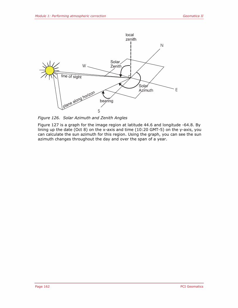
Module 1: Performing atmospheric correction Geomatica II
Page 162 PCI Geomatics
Figure 126. Solar Azimuth and Zenith Angles
Figure 127 is a graph for the image region at latitude 44.6 and longitude -64.8. By
lining up the date (Oct 8) on the x-axis and time (10:20 GMT-5) on the y-axis, you
can calculate the sun azimuth for this region. Using the graph, you can see the sun
azimuth changes throughout the day and over the span of a year.

Module 1: Performing atmospheric correction Geomatica II
PCI Geomatics Page 163
Figure 127. Sun Azimuth Diagram for Latitude 47, Longitude -783
To set the radiometric information
Although Focus automatically reads radiometric information from the file’s
metadata, review the radiometric band details to ensure that the bands are correctly allocated to the appropriate channel.
3 Reference: jgiesen.de/azimuth
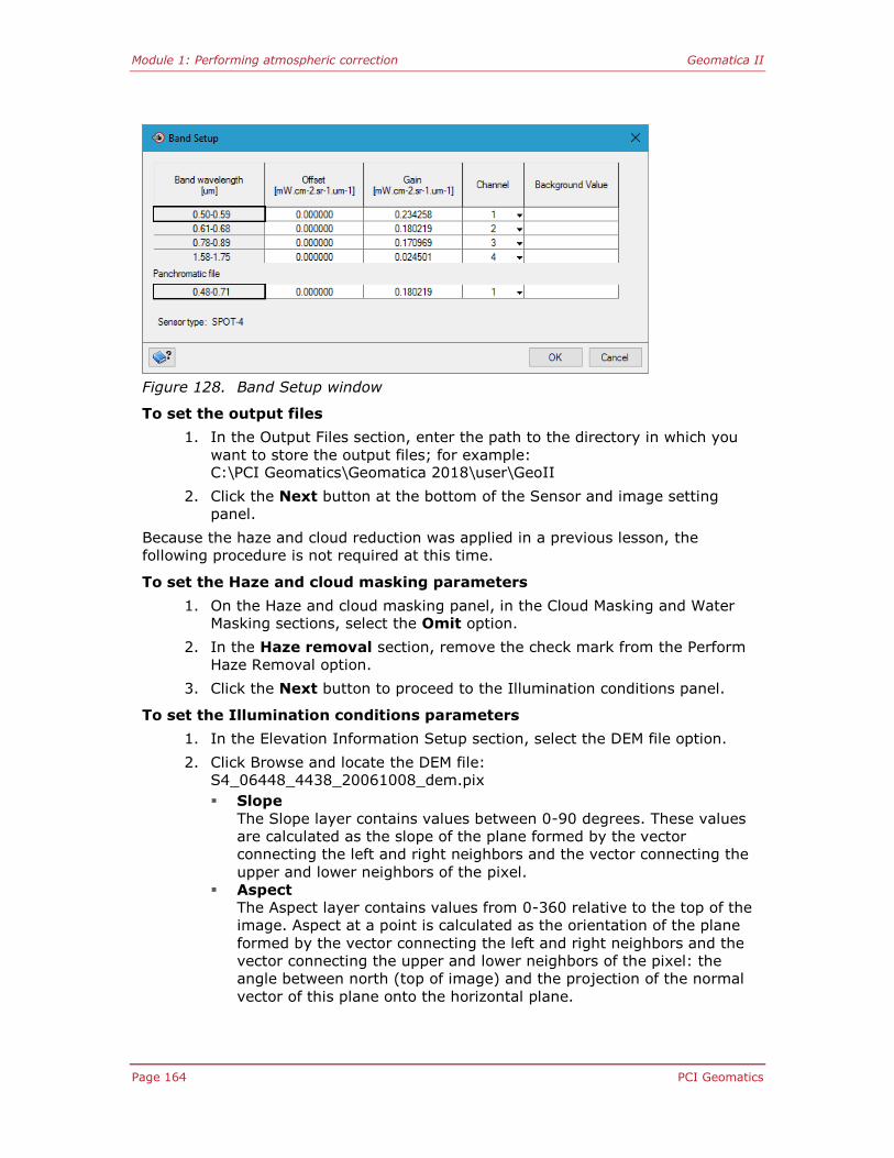
Module 1: Performing atmospheric correction Geomatica II
Page 164 PCI Geomatics
Figure 128. Band Setup window
To set the output files
1. In the Output Files section, enter the path to the directory in which you
want to store the output files; for example: C:\PCI Geomatics\Geomatica 2018\user\GeoII
2. Click the Next button at the bottom of the Sensor and image setting
panel.
Because the haze and cloud reduction was applied in a previous lesson, the
following procedure is not required at this time.
To set the Haze and cloud masking parameters
1. On the Haze and cloud masking panel, in the Cloud Masking and Water Masking sections, select the Omit option.
2. In the Haze removal section, remove the check mark from the Perform
Haze Removal option.
3. Click the Next button to proceed to the Illumination conditions panel.
To set the Illumination conditions parameters
1. In the Elevation Information Setup section, select the DEM file option.
2. Click Browse and locate the DEM file:
S4_06448_4438_20061008_dem.pix
Slope
The Slope layer contains values between 0-90 degrees. These values
are calculated as the slope of the plane formed by the vector
connecting the left and right neighbors and the vector connecting the
upper and lower neighbors of the pixel.
Aspect
The Aspect layer contains values from 0-360 relative to the top of the
image. Aspect at a point is calculated as the orientation of the plane
formed by the vector connecting the left and right neighbors and the
vector connecting the upper and lower neighbors of the pixel: the
angle between north (top of image) and the projection of the normal
vector of this plane onto the horizontal plane.

Module 1: Performing atmospheric correction Geomatica II
PCI Geomatics Page 165
Sky View
The Sky View layer is calculated with a ray tracing program and ranges
from 0 to 1, with 1 indicating a full hemispherical view. The Sky View
factor determines the fraction of the hemispherical diffuse sky flux and
determines the fraction of radiation reflected from surrounding
mountains onto the considered pixel.
Shadow
The shadow layer is a binary file where shadow pixels are coded with 0
and sunlit pixels with 1. It includes self-shadowing and cast shadow
effects. Self-shadowing consists of pixels oriented away from the sun
with slopes steeper than the solar elevation angle. The cast shadow
calculation is based on a ray tracing algorithm and includes shadow
regions caused by higher surrounding mountains.
3. Accept the default Calculate option for the Illumination Map.
4. Click the Next button to proceed to the Visibility and ground reflectance
panel.
To set the Visibility and ground reflectance parameters
1. In the Atmospheric Information section, set the Aerosol Type to
Maritime.
Due to the proximity of the area in the image to the Atlantic Ocean, the
atmosphere contains salt.
2. Set the Condition to Fall/Spring.
3. The Satellite Viewing Geometry information is automatically obtained from
the file’s metadata. Review the information to ensure that it is correct.
4. In the Visibility Map section, select the Use constant visibility option and
enter a visibility value of 30 km.
5. In the Reflectance Correction section, select the Correct for adjacency
effects check box.
Adjacency is the effect of backscattering on neighboring pixels. It is used
to more accurately specify the atmospheric conditions at the time the
image was taken. This is a value in kilometers and can be set to 0, which
means it will not take the adjacency effect into consideration. The default value of 1km is optimal for most cases.

Module 1: Performing atmospheric correction Geomatica II
Page 166 PCI Geomatics
Figure 129. Atmospheric Correction window Visibility and ground reflectance
parameters
6. Accept the default state of the check boxes (cleared) in the Output
section.
Value-added output
You have the option to create value added products when running
atmospheric correction. These include Soil-Adjusted Vegetation Index
(SAVI), Leaf-Area Index (LAI), Fraction of Absorbed Radiation (FPAR),
Surface Albedo, and Absorbed Solar Radiation. It is also possible to
create other value-added layers which require the thermal image band
with the input data. These include Thermal Flux Difference, Ground
Heat Flux, Latent Heat, Sensible Heat and Net Radiation.
7. Click the Run button.
The Atmospheric Correction process begins. When the correction is
finished, Focus displays the results in the viewer.
The result of the atmospheric correction is a reflectance image stored in a 32-bit
channel.
Lesson summary
In this lesson you:
Set up for atmospheric correction using ATCOR
Ran atmospheric correction on a SPOT-4 scene