Geography, Uncertainty, and Polarization∗

Nolan McCarty†, Jonathan Rodden‡, Boris Shor§,

Chris Tausanovitch¶, and Chris Warshaw∥

April 7, 2014

Abstract

Using new data on roll-call votes and public opinion in U.S. state legislative dis-

tricts, we explain how ideological polarization within districts can lead to legislative

polarization. Many of the seemingly “moderate” districts in suburbs and smaller cities

that switch hands between Democrats and Republicans are internally polarized. The

ideological distance between Democrats and Republicans within these districts is often

greater than the distance between liberal cities and conservative rural areas. We present

a theoretical model in which intra-district ideological polarization causes candidates to

be uncertain about the ideological location of the median voter, thereby reducing their

incentives for platform moderation. We then demonstrate that in otherwise identical

districts, the difference in roll-call voting behavior between Democratic and Republican

state legislators is a function of within-district ideological heterogeneity. Accounting

for the subtleties of political geography can help explain the juxtaposition of a polarized

legislature and a moderate mass public.

∗Paper prepared for the Conference on the Causes and Consequences of Policy Uncertainty at PrincetonUniversity. An earlier version of the paper was presented at the 2013 Annual Meetings of the AmericanPolitical Science Association. We thank Project Votesmart for access to NPAT survey data. The roll calldata collection has been supported financially by the Russell Sage Foundation, the Princeton UniversityWoodrow Wilson School, the Robert Wood Johnson Scholar in Health Policy program, and NSF GrantsSES-1059716 and SES-1060092. Special thanks are due to Michelle Anderson and Peter Koppstein forrunning the roll-call data collection effort. We also thank the following for exemplary research assistance:Steve Rogers, Michael Barber, and Chad Levinson.

†Professor, Department of Politics, Princeton University, nmccarty@princeton.edu‡Professor, Department of Political Science and Senior Fellow, Hoover Institution, Stanford University,

jrodden@stanford.edu§Assistant Professor, Harris School of Public Policy Studies, University of Chicago, boris@bshor.com¶Assistant Professor, Department of Political Science, UCLA, ctausanovitch@ucla.edu∥Assistant Professor, Department of Political Science, Massachusetts Institute of Technology,

cwarshaw@mit.edu

1

Introduction

One of the enduring puzzles in the study of American politics is the juxtaposition of an

increasingly polarized Congress with an apparently stable and centrist electorate (Fiorina

2010). After failing to find a link between polarization in Congress and the polarization

of policy preferences in national surveys, researchers are turning away from the ideology of

the mass public, looking instead at institutional features like primaries, agenda control in

the legislature, and redistricting that may have led to increased Congressional polarization

(Fiorina and Abrams 2008).

This paper brings attention back to the distribution of ideology in the mass public with

new data and an alternative theoretical approach. Previous explanations for polarization

focus, quite naturally, on variation across the nation as a whole, or on the average or median

of traits of citizens in each district (McCarty, Poole and Rosenthal 2006; Jacobson 2004;

Levendusky 2009). This work follows from a long literature on representation that builds

on Black’s median voter theorem (Black 1948), which implies that the preferences of large

groups can be characterized by that of the median individual.

The great majority of work in this area, however, finds that the median voter is an inade-

quate predictor of candidate or legislator positions (Ansolabehere, Snyder Jr and Stewart III

2001; Bafumi and Herron 2010; Clinton 2006; Miller and Stokes 1963). This paper builds

on a nascent literature that focuses on the distribution of preferences across voters within

districts rather than the median or mean (Gerber and Lewis 2004; Levendusky and Pope

2010). Our theory builds on the work of Calvert (1985) and Wittman (1983). We develop a

model in which candidates with ideological preferences must choose platforms in the presence

1

of uncertainty over the median voter. When candidates are uncertain about the ideological

location of the median voter, they shade their platforms toward their own–or their party’s–

more extreme ideological preferences. Our key insight is that uncertainty about the median

voter is driven in part by the ideological distribution of preferences in the district and the

mapping of ideology to turnout from one election to the next. The intuition is that when

there is a large mass of voters around the district median, even though turnout is volatile,

the median voter on election day will be within a narrow range, and candidates cannot de-

viate very far from it. In contrast, when voters are more evenly distributed throughout the

ideological spectrum or even polarized into a bimodal distribution, there is more uncertainty

about the identity of the median voter on election day, and hence weaker incentives for the

candidates to strategically suppress their own ideology in pursuit of victory.

Existing research on polarization in the United States focuses primarily on attempting

to explain a single time-series: the dramatic growth of polarization in the United States

Congress (Poole and Rosenthal 1997). Unfortunately, the focus on Congress means that

polarization is increasing along with many endogenous co-variates since the 1960s, and the

time series may reflect strategic changes in agenda control by the parties. Moreover, most of

the increase in polarization occurred prior to the years for which reliable estimates of voter

ideology can be created at the district level. Drawing on the vast data collection efforts of

Shor and McCarty (2011), we turn away from the traditional analysis of change over time

in the U.S. Congress, focusing instead on the considerable cross-sectional variation in state

legislative polarization. As we demonstrate below, some states are even more polarized than

the U.S. Congress, while others are much less so.

Our explanation for this heterogeneity focuses squarely on an obvious blind spot in the

2

literature on polarization: the geography of preferences. The focus on the overall national

distribution of preferences–the dominant frame of previous work–is strangely misplaced in an

electoral system with winner-take-all electoral districts. Legislative candidates should care

only about the distribution of preferences in their own districts. If platforms of candidates

and roll-call voting behavior of incumbents are responsive to the district median voter,

ideological polarization across districts should correspond to polarization in roll-call voting.

Indeed, we find some fragile cross-section evidence to this effect: the states with the largest

ideological gap between voters in left-wing and right-wing districts also demonstrate the

largest ideological distance between Democratic and Republican legislators.

Ideological polarization across districts within states is only part of the story, however,

and only a prologue to this paper’s main contribution. In many states, a district-level version

of Fiorina’s puzzle remains: there is a large density of districts where the median or average

voter is quite moderate, but the voting behavior of the representative is extreme, and the

legislature is far more sharply polarized than is the distribution of district medians. In what

follows, our model of uncertainty over the median legislator will help resolve this puzzle.

After presenting our theory, we turn to an empirical analysis of roll-call votes of state

legislators. Building on the work of McCarty, Poole and Rosenthal (2009), we match dis-

tricts that are as similar as possible on all dimensions but partisan control, showing that 1)

as in the U.S. Congress, there is considerable divergence in roll-call voting across otherwise

identical districts controlled by Democrats and Republicans, and 2) this inter-district diver-

gence is a function of within-district ideological polarization as well as more direct proxies

for uncertainty over the identity of the district median voter.

We conclude with a discussion of the implications of these findings for the polarization

3

literature. It is quite plausible that the rise of polarization in the U.S. Congress has also been

driven by increasing within-district polarization associated with demographic and residen-

tial sorting in recent decades. Moreover, our results suggest skepticism about redistricting

reforms aimed at creating more ideologically heterogeneous districts as a cure for legislative

polarization McCarty, Poole and Rosenthal (2009); McGhee et al. (2013); Kousser, Phillips

and Shor (2013). Finally, the utility of these results for explaining polarization suggest that

future research on representation should take seriously the idea that other features of the

distribution of preferences within districts may be important for determining legislator po-

sitions. Legislators do not answer to a single principle or compete with a fixed challenger

(Besley 2007). They must balance competing strategic considerations as well as their own

preferences in deciding what policy positions to uphold (Fiorina 1974).

Polarization Between andWithin Districts: Stylized Facts

The geographic distribution of ideology within states

We begin by establishing some stylized facts that motivate the remainder of the paper. First,

we examine the geographic distribution of ideology within states. One of the obstacles to

previous research on this topic is that we have lacked good measures of the mass public’s

ideology at the individual level in each state. However, Tausanovitch and Warshaw (2013)

have created a bridge between several surveys, allowing them to dramatically increase the

size of survey samples within small geographic areas, making it possible for the first time

to characterize not only the mean or median, but also the nature of the distribution of

4

Figure 1: Ideological polarization within and between districts

.6 .8 1 1.2 1.4

WAHI

COAZ

WYNMMNCAIA

VAMTMEWITXNHMOFL

GAIL

CTMIUTNCDEOHMDPAID

NETNSDSCKSIN

OKLANJ

MSNDARNYALKYRI

WV

Overall SD of ideology SD of district mediansMean of within−district SD

ideological preferences within states and even legislative districts. Using survey responses on

a battery of policy questions in the super-survey, we create an ideological preference scale

for over 350,000 respondents. We are then able to characterize some basic features of the

geographic distribution of ideology in the United States, summarized in Figure 1.

We use these new data to examine three inter-related concepts. First, we measure the

heterogeneity of each state’s ideology based on the standard deviation of citizens’ ideology

within states.1 These estimates are shown with the green dots in Figure 1. The state

1This scale corresponds closely to the measure of state ideology heterogeneity in Levendusky and Pope(2010).

5

with the greatest ideological heterogeneity is Washington, and the state with the narrowest

spread is West Virginia. Some of the most ideologically heterogeneous states are in the West:

Washington, Colorado, Arizona, Wyoming, New Mexico, and California. Some of the least

heterogeneous states are some of the very conservative states of the South, along with some

of the very liberal states of the Northeast.

Next, in order to capture between-district polarization, we take the median of our ide-

ological scale within each state senate district, and calculate the standard deviation across

all districts in the state. We plot this indicator with the orange dots in Figure 1. Finally,

in order to capture within-district polarization, we calculate the standard deviation of the

ideological scale within each state senate district, and then average across the standard

deviations of all districts in the state. This indicator is represented in blue in Figure 1.

One might guess that the ideological polarization of states like Washington, Colorado, or

Minnesota comes from the vast ideological gulf between Seattle, Denver/Boulder, or Min-

neapolis and the surrounding exurban and rural peripheries. However, Figure 1 shows that

between-district polarization is only weakly correlated with polarization in the mass public.

Within-district polarization is far larger in magnitude than between-district polarization,

and more closely associated with the mass public’s level of polarization. For instance, West

Virginia’s low overall level of ideological polarization is explained not by the distance between

liberal and conservative parts of the state– which is actually relatively large– but rather, by

its unusually low level of ideological heterogeneity within districts. Some of the ideologically

polarized Western states do demonstrate relatively large ideological distance between the

medians of their liberal urban districts and conservative rural districts, but the bigger story

is the fact that voters are ideologically far apart within a wide cross-section of districts.

6

Where are the polarized districts?

Next, we examine the relationship between the ideology of the median voter in each district

and its heterogeneity. Figure 2 plots our measure of the standard deviation of ideology for

each state senate district on the horizontal axis, and our estimate of mean ideology of the

district on the horizontal axis. The left side of the inverted U shape of the lowess plot in

Figure 2 shows that the far-left urban enclaves are ideologically relatively homogeneous. The

same is true for the conservative exurban and suburban districts on the right side of the plot.

Figure 2: Average district ideology and within-district polarization

1.0

1.2

1.4

1.6

−1 0 1Median Citizen Ideology

Unc

erta

inty

Average district ideology and within−district polarization

The most internally polarized districts are those in the middle of the ideological spectrum.

In other words, the districts with the most moderate ideological means– the “purple” districts

where the presidential vote share is most evenly split– are the places where the electorate is

most deeply polarized. These are the districts that switch back and forth between parties in

7

close elections and determine which party controls the state legislature.

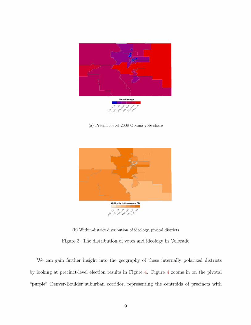
To see this more clearly, it is useful to take a closer look at the distribution of ideology

in a highly polarized state. The panel on the left of Figure 3 displays our estimates of

ideological means across the Colorado state senate districts, and the panel on the right

displays the within-district standard deviation of the ideological scale. It shows that most

of the ideologically “moderate” districts in the state, colored in shades or purple on the left,

are also among the most internally polarized (darker shades of orange on the right).

8

Mean ideology

-1.3

7 - -0.3

2

-0.3

1 - -0.1

3

-0.1

2 - 0

.00

0.0

1 - 0

.12

0.1

3 - 0

.24

0.2

5 - 0

.58

(a) Precinct-level 2008 Obama vote share

Within-district ideological SD

0.0

0 - 1

.17

1.1

8 - 1

.24

1.2

5 - 1

.28

1.2

9 - 1

.33

1.3

4 - 1

.39

1.4

0 - 1

.81

(b) Within-district distribution of ideology, pivotal districts

Figure 3: The distribution of votes and ideology in Colorado

We can gain further insight into the geography of these internally polarized districts

by looking at precinct-level election results in Figure 4. Figure 4 zooms in on the pivotal

“purple” Denver-Boulder suburban corridor, representing the centroids of precincts with

9

colored dots. The numbers of the districts with the most ideologically moderate means are

displayed in Figure 4, and these match up with kernel densities, displayed in Figure 4, of the

distribution of our ideological scale within each corresponding district.

The Denver area is typical of many other U.S. metropolitan areas. Just outside the city

center is a ring of ideologically moderate suburbs where the Obama vote share was slightly

above 50 percent, and we see in Figure 4 that in some of them, for instance 19, 20, and 21,

most of the precincts themselves are varying shades of purple. Nevertheless, we see in Figure

4 that the internal ideological distributions are sharply polarized.

Figure 4 also portrays another genus of internally polarized district. Districts 15 and 16

are examples of more sparsely populated districts that contain sizable, residentially segre-

gated pockets of both Democrats and Republicans. This phenomenon is most often found

when exurban or rural conservative areas contain concentrated pockets of liberal Democrats,

such as college towns, ski towns, 19th century manufacturing or natural resource extraction

centers, or concentrations of racial minorities.

10

Obama 2008 vote share

0.0

0 - 0

.28

0.2

9 - 0

.44

0.4

5 - 0

.54

0.5

5 - 0

.63

0.6

4 - 0

.76

0.7

7 - 1

.00

15

16

17

19

2021

(a) Precinct-level 2008 Obama vote share

.05

.1.1

5.2

.25

−4 −2 0 2 4

15

.05

.1.1

5.2

.25

−4 −2 0 2 4

16

.05

.1.1

5.2

.25

.3

−4 −2 0 2 4

17

.05

.1.1

5.2

.25

−4 −2 0 2 4

19

.05

.1.1

5.2

.25

−4 −2 0 2 4

20

.05

.1.1

5.2

.25

−4 −2 0 2 4

21

(b) Within-district distribution of ideology, pivotal districts

Figure 4: Within-district distributions of votes and ideology, selected Colorado Senate dis-tricts 11

Does ideological polarization correspond to legislative polarization?

These data enable a new approach to what is becoming a classic question in American poli-

tics: does ideological polarization in the mass public correspond to ideological polarization

in legislatures? The current literature answers with a tentative “no,” based on time series

analysis of the U.S. Congress, where legislative polarization has grown but the ideological

distance between Democrats and Republicans in the mass public has not.

As discussed above, Shor and McCarty (2011) have estimated ideal points of members

of state legislatures from a large data set of roll-call votes covering several years. As a first

cut, let us examine the shapes of the cross-district distributions of ideology and roll-call

votes. If legislative polarization is a function of ideological polarization across districts, we

might expect to see the familiar bimodal distribution of legislator ideal points mirrored in

the distribution of ideology across districts.

Figure 5: Distributions of roll-call votes and district ideology

Legislators Individuals

0.0

0.2

0.4

0.6

−2 −1 0 1 2 3 −2 −1 0 1 2 3Ideology

Figure 5 displays kernel densities of both measures across all state upper chambers:

12

there is sharp divergence between the roll-call votes of Democrats and Republicans, but the

distribution of ideology across districts has a single peak. The disjuncture is even more

extreme when one examines these distributions separately for each state. Thus Fiorina’s

(2010) puzzle reappears at the district level: there is a large density of moderate districts,

but in many states the middle of the ideological distribution is not well represented in state

legislatures.

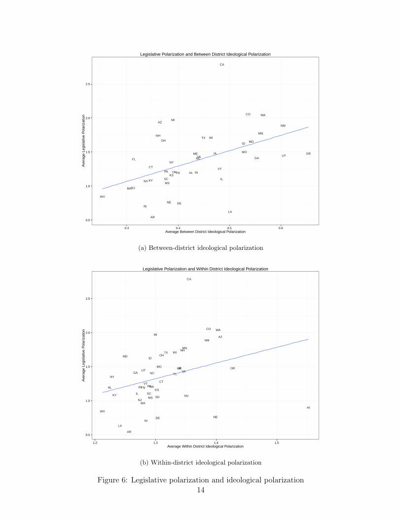
Next, we examine cross-state variation in the polarization of legislatures, which we define

here as the distance in ideal point estimates between the mean Democrat and the mean Re-

publican in the legislature. In Figure 6, we plot the degree of legislative polarization against

the between- and within-district measures of ideological polarization introduced above. In-

deed, there is correspondence between ideological polarization in the mass public and the

polarization of roll-call votes in the legislature. Not only is legislative polarization corre-

lated with between-district ideological polarization, but the states with the highest levels

of within-district polarization, like California, Colorado, and Washington, are also clearly

those with the highest levels of legislative polarization. In the states like West Virginia and

Louisiana, where public opinion is not very polarized within districts, the Democrats and

Republicans in the legislature are not very distinctive.

13

AL

AR

AZ

CA

CO

CT

DE

FL GA

IA

ID

IL

INKS

KY

LA

MA

MD

ME

MI

MN

MO

MS

NC

NE

NH

NJ

NM

NV

NY

OH

OK

OR

PA

RI

SC

TN

TX

UTVA

VT

WA

WI

WV

0.5

1.0

1.5

2.0

2.5

0.3 0.4 0.5 0.6Average Between District Ideological Polarization

Ave

rage

Leg

isla

tive

Pol

ariz

atio

n

Legislative Polarization and Between District Ideological Polarization

(a) Between-district ideological polarization

AL

AR

AZ

CA

CO

CT

DE

FLGA

HI

IA

ID

IL

INKS

KY

LA

MA

MD

ME

MI

MN

MO

MS

NC

NE

NH

NJ

NM

NV

NY

OH

OK

OR

PA

RI

SCSD

TN

TX

UT VA

VT

WA

WI

WV

0.5

1.0

1.5

2.0

2.5

1.2 1.3 1.4 1.5Average Within District Ideological Polarization

Ave

rage

Leg

isla

tive

Pol

ariz

atio

n

Legislative Polarization and Within District Ideological Polarization

(b) Within-district ideological polarization

Figure 6: Legislative polarization and ideological polarization

14

These stylized facts motivate the remainder of the paper. In the middle of each states’ dis-

tribution of districts lies a set of potentially pivotal districts that are ideologically moderate

on average, but where voters are polarized within. Moreover, this within-district ideological

polarization is a good predictor of polarization in state legislatures.

But given the logic of the median voter, why would electoral competition in these pivotal

but polarized districts generate such polarized legislative representation? The remainder of

the paper develops a simple intuition: when turnout is variable and difficult to predict, a

heterogeneous internal distribution of ideology, such as the distributions displayed in Figure

4 above, creates uncertainty over the spatial location of the median voter. When a district

is internally polarized, a moderate shift in the mapping of ideology to turnout– perhaps

driven by national or statewide trends– can lead to a substantial shift in the location of

the median voter. Relative to a district with a large density of moderates in the middle

of the internal distribution, candidates in such polarized districts face weaker incentives for

platform convergence.

The Model

Following Wittman (1983) and Calvert (1985), assume that there are two political parties

who have policy preferences on a single dimension. Let θL < θR be the ideal points of party

L and R respectively. The preferences of party L are given by a concave utility function

uL(x) where uL is maximized at zero for x = θL and decreasing in x > θL. Similarly, the

utility of party R is given by uR(x) which is maximized at x = θR and increasing for x < θR.2

2Outcomes outside the interval [θL, θR] involve dominated strategies.

15

We assume that the parties are uncertain about the distribution of voter preferences.

But they share common beliefs that the ideal point of the median (and decisive) voter m

is given by probability function F where F (θL) = 0 and F (θR) = 1.3 We assume that the

median voter has single-peaked preferences around m.

Prior to the election, parties L and R commit to platforms xL and xR.4 Voter m votes

for the party with the closest platform. Therefore, party L wins if and only if m ≤ xL+xR

2.

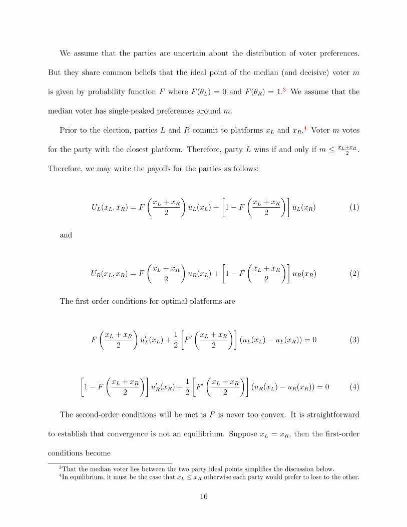
Therefore, we may write the payoffs for the parties as follows:

UL(xL, xR) = F

(xL + xR

2

)uL(xL) +

[1− F

(xL + xR

2

)]uL(xR) (1)

and

UR(xL, xR) = F

(xL + xR

2

)uR(xL) +

[1− F

(xL + xR

2

)]uR(xR) (2)

The first order conditions for optimal platforms are

F

(xL + xR

2

)u′L(xL) +

1

2

[F ′

(xL + xR

2

)](uL(xL)− uL(xR)) = 0 (3)

[1− F

(xL + xR

2

)]u′R(xR) +

1

2

[F ′

(xL + xR

2

)](uR(xL)− uR(xR)) = 0 (4)

The second-order conditions will be met is F is never too convex. It is straightforward

to establish that convergence is not an equilibrium. Suppose xL = xR, then the first-order

conditions become

3That the median voter lies between the two party ideal points simplifies the discussion below.4In equilibrium, it must be the case that xL ≤ xR otherwise each party would prefer to lose to the other.

16

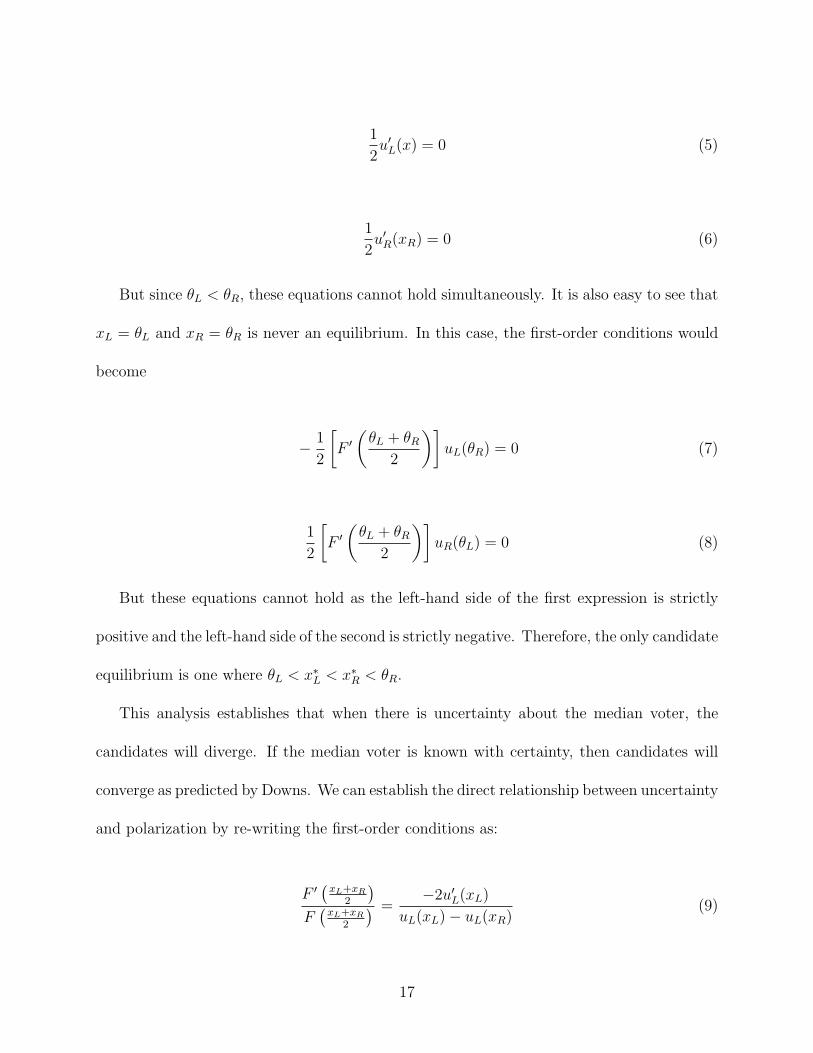
1

2u′L(x) = 0 (5)

1

2u′R(xR) = 0 (6)

But since θL < θR, these equations cannot hold simultaneously. It is also easy to see that

xL = θL and xR = θR is never an equilibrium. In this case, the first-order conditions would

become

− 1

2

[F ′

(θL + θR

2

)]uL(θR) = 0 (7)

1

2

[F ′

(θL + θR

2

)]uR(θL) = 0 (8)

But these equations cannot hold as the left-hand side of the first expression is strictly

positive and the left-hand side of the second is strictly negative. Therefore, the only candidate

equilibrium is one where θL < x∗L < x∗

R < θR.

This analysis establishes that when there is uncertainty about the median voter, the

candidates will diverge. If the median voter is known with certainty, then candidates will

converge as predicted by Downs. We can establish the direct relationship between uncertainty

and polarization by re-writing the first-order conditions as:

F ′ (xL+xR

2

)F(xL+xR

2

) =−2u′

L(xL)

uL(xL)− uL(xR)(9)

17

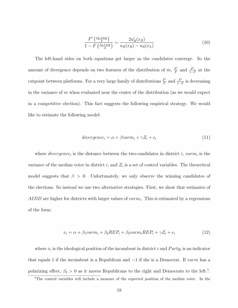
F ′ (xL+xR

2

)1− F

(xL+xR

2

) =2u′

R(xR)

uR(xR)− uR(xL)(10)

The left-hand sides on both equations get larger as the candidates converge. So the

amount of divergence depends on two features of the distribution of m, F ′

Fand F ′

1−Fat the

cutpoint between platforms. For a very large family of distributions F ′

Fand F ′

1−Fis decreasing

in the variance of m when evaluated near the center of the distribution (as we would expect

in a competitive election). This fact suggests the following empirical strategy. We would

like to estimate the following model:

divergencei = α + βvarmi + γZi + ϵi (11)

where divergencei is the distance between the two-candidates in district i, varmi is the

variance of the median voter in district i, and Zi is a set of control variables. The theoretical

model suggests that β > 0. Unfortunately, we only observe the winning candidates of

the elections. So instead we use two alternative strategies. First, we show that estimates of

AIDD are higher for districts with larger values of varmi. This is estimated by a regressions

of the form:

xi = α+ β1varmi + β2REPi + β3varmiREPi + γZi + ϵi (12)

where xi is the ideological position of the incumbent in district i and Partyi is an indicator

that equals 1 if the incumbent is a Republican and −1 if she is a Democrat. If varm has a

polarizing effect, β3 > 0 as it moves Republicans to the right and Democrats to the left.5.

5The control variables will include a measure of the expected position of the median voter. In the

18

Second, following McCarty, Poole and Rosenthal (2009) and Shor and McCarty (2011) we use

matching techniques to estimate the average district divergence for districts with different

levels of varmi.

An Empirical Exploration of Within-District Divergence

As we indicated in the last section, the lack of observations of losing challengers complicates

our analysis. We follow the approach of McCarty et al (2009), who decompose partisan

polarization into roughly two components. The first part, which they term intradistrict

divergence is simply the difference between how Democratic and Republican legislators would

represent the same district. The remainder, which they term sorting , closely related to

what we refer to above as between-district polarization, is the result of the propensity for

Democrats to represent liberal districts and for Republicans to represent conservative ones.

To formalize the distinction between divergence and sorting, we can write the difference

in party mean ideal points as

E(x |R)− E(x |D ) =

∫ [E(x |R, z )

p(z)

p− E(x |D, z )

1− p(z)

1− p

]f(z)dz

where x is an ideal point, R and D are indicators for the party of the representative, and z

is a vector of district characteristics. We assume that z is distributed according to density

function f and that p(z) is the probability that a districts with characteristics z elects a

Republican. The term p is the average probability of electing a Republican. The average

difference between a Republican and Democrat representing a district with characteristics z,

matching analysis, the expected median is one of the covariates on which we match.

19

E(x |R, z )−E(x |D, z ), captures the intradistrict divergence, while variation in p(z) captures

the sorting effect.

Estimating the AIDD is analogous to estimating the average treatment effect of the

non-random assignment of party affiliations to representatives. There is a large literature

discussing alternative methods of estimation for this type of analysis. For now we assume

that the assignment of party affiliations is based on observables in the vector z. If we assume

linearity for the conditional mean functions, i.e., E(x|R, z) = β1+β2R+β3x, we can estimate

the AIDD as the OLS estimate of β2 . But following the suggestion of Wooldridge (2002), we

include interactions of R with z in mean deviations to allow for some forms of non-linearity.

Mean deviating z before interacting with R insures that that the AIDD is the coefficient on

R.

Our claim is that the average intradistrict divergence is a function of uncertainty over the

location of the median voter within districts. This follows directly from the Wittman-Calvert

model. For the purposes of our empirical analysis, the key assumption is that uncertainty

over the position of the median is greater in more heterogenous districts. Legislators are

familiar with the distributions of preferences in their district, but uncertainty stems from

many sources. Changing preferences, turnout, and changes in the composition of the districts

can all have an effect. These “shocks” may be non-independent, inducing uncertainty over

the median even in large samples.6 However, in homogenous electorates, even large shocks

will fail to move the median voter. In more heterogenous electorates, small shocks may

be sufficient. For this reason, within-district ideological heterogeneity is a good proxy for

6According to the Wittman-Calvert model, even a small amount of uncertainty can induce divergence,so even if shocks are independent, candidates will diverge.

20

uncertainty over the median voter.

We use two measures of ideological heterogeneity. The first and most straightforward was

already displayed in some of the graphs above: the standard deviation of preferences in the

electorate (Gerber and Lewis 2004; Levendusky and Pope 2010). We estimate this measure

for every state senate district in the country using the large dataset of citizens’ ideal points

from Tausanovitch and Warshaw (2013). The second measure is a more direct measure of

the uncertainty over the median voter in each district. In order to measure uncertainty over

the median, we bootstrapped 20 different samples from each district and fixed the number of

respondents at 40 in each district.7 This allows us to hold variation in sampling error fixed

across districts. In each simulation, we estimated the median ideal point in each district.

Then, across all the simulations, we estimated the standard deviation of the median. This

measure captures uncertainty over the median voter in each district.8

We present our empirical results in Table 1. Results using the heterogeneity measure are

presented in columns 1 and 2, while the results using the measure of uncertainty over the

median are presented in column 3 and 4. Also, columns 1 and 3 use measures that include

voters only, whereas columns 2 and 4 use the entire district-level sample.

No matter which measure we use, average intradistrict divergence is clearly a function of

ideological heterogeneity in the district. Controlling for mean ideology, presidential vote, and

a variety of demographic covariates, the difference between the roll-call voting behavior of

Democrats and Republicans within states is largest in districts that are most heterogeneous,

and smallest in districts that have the most ideologically homogeneous. To get a better

7We were only able to calculate this measure of uncertainty for districts where had more than 40 respon-dents in our data, which forced us to drop about 50% of state senate districts.

8Note that this measure is a function of the percentage of “moderate” voters in each district that lienear the median.

21

idea of the size, of the effect, consider the first column of Table 1. A 1 standard deviation

reduction in the voter heterogeneity - the standard deviation of the distribution of voters-

leads to a reduction of .35 in the average interdistrict divergence. Figure 7(a) shows what this

means more vividly. A district with heterogeneity less than one can expect to be represented

by a moderate, regardless of party. In stark contrast, districts with heterogeneity of 1.75 can

expect to be represented by a legislator who is from the extremes of their party.

One possible objection to this result is that it may be endogenous. State legislators are

themselves in charge of the districting process in many states. It could be the case that more

extreme legislators have more heterogenous districts because they designed the districts this

way. There is reason to doubt this alternative explanation for our results. If this were

the case, then it seems that moderates are being relegated to unsafe districts- precisely the

opposite of what you would expect if moderates are able to leverage their pivotal position

in the legislative process. However, we cannot a priori rule out the idea that districting is

playing a role in producing these results. as a robustness check, we limit the sample to only

those states with non-partisan districting commissions. Table 2 reports the results of this

analysis. Our results with regard to our first measure of heterogeneity are robust to this

limitation of our sample. However, our results with respect to our second measure are no

longer significant. Although we suspect that this is due to lower variability in this measure,

we cannot decisively rule out a role for gerrymandering.

Because these functional forms used in the above analysis are somewhat restrictive, we

also use matching estimators to calculate the AIDD. Intuitively, these estimators match

observations from a control and treatment group that share similar characteristics z and

then compute the average difference in roll-call voting behavior for the matched set. We use

22

Table 1: Uncertainty/Legislator Score Models (OLS)

Dependent variable:

Legislator Score

(1) (2) (3) (4)

Republican −0.68∗∗∗ −0.79∗∗∗ 0.89∗∗∗ 0.75∗∗∗

(0.19) (0.14) (0.08) (0.06)

Heterogeneity Voters −0.35∗∗∗

(0.07)

Heterogeneity Citizens −0.67∗∗∗

(0.07)

Uncertainty Voters −0.48∗∗∗

(0.07)

Uncertainty Citizens −0.77∗∗∗

(0.08)

Median Citizen Ideology 0.33∗∗∗ 0.32∗∗∗ 0.35∗∗∗ 0.36∗∗∗

(0.03) (0.02) (0.03) (0.02)

R Pres Vote 2008 1.26∗∗∗ 1.29∗∗∗ 1.19∗∗∗ 1.14∗∗∗

(0.12) (0.08) (0.11) (0.07)

Heterogeneity Voters * R 1.19∗∗∗

(0.12)

Heterogeneity Citizens * R 1.51∗∗∗

(0.10)

Uncertainty Voters * R 0.58∗∗∗

(0.10)

Uncertainty Citizens * R 1.43∗∗∗

(0.11)

Citizen Ideology * R −0.02 −0.08∗∗ −0.10∗∗ −0.13∗∗∗

(0.05) (0.03) (0.05) (0.03)

R Pres Vote 2008 * R 0.25 −0.08 0.31∗ 0.05(0.17) (0.12) (0.17) (0.11)

Observations 3,550 5,870 3,550 5,870R2 0.83 0.82 0.83 0.82Adjusted R2 0.83 0.82 0.83 0.82Residual Std. Error 0.38 (df = 3542) 0.38 (df = 5862) 0.39 (df = 3542) 0.38 (df = 5862)

Note: ∗p<0.1; ∗∗p<0.05; ∗∗∗p<0.01

23

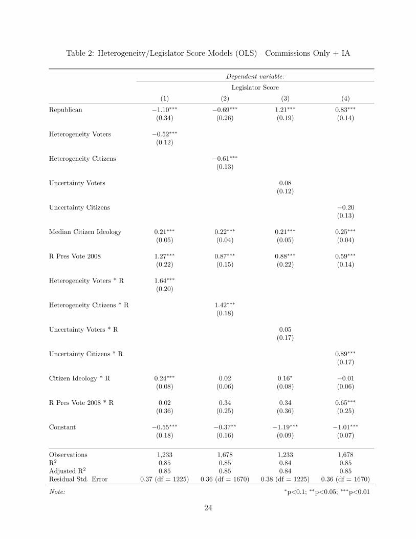
Table 2: Heterogeneity/Legislator Score Models (OLS) - Commissions Only + IA

Dependent variable:

Legislator Score

(1) (2) (3) (4)

Republican −1.10∗∗∗ −0.69∗∗∗ 1.21∗∗∗ 0.83∗∗∗

(0.34) (0.26) (0.19) (0.14)

Heterogeneity Voters −0.52∗∗∗

(0.12)

Heterogeneity Citizens −0.61∗∗∗

(0.13)

Uncertainty Voters 0.08(0.12)

Uncertainty Citizens −0.20(0.13)

Median Citizen Ideology 0.21∗∗∗ 0.22∗∗∗ 0.21∗∗∗ 0.25∗∗∗

(0.05) (0.04) (0.05) (0.04)

R Pres Vote 2008 1.27∗∗∗ 0.87∗∗∗ 0.88∗∗∗ 0.59∗∗∗

(0.22) (0.15) (0.22) (0.14)

Heterogeneity Voters * R 1.64∗∗∗

(0.20)

Heterogeneity Citizens * R 1.42∗∗∗

(0.18)

Uncertainty Voters * R 0.05(0.17)

Uncertainty Citizens * R 0.89∗∗∗

(0.17)

Citizen Ideology * R 0.24∗∗∗ 0.02 0.16∗ −0.01(0.08) (0.06) (0.08) (0.06)

R Pres Vote 2008 * R 0.02 0.34 0.34 0.65∗∗∗

(0.36) (0.25) (0.36) (0.25)

Constant −0.55∗∗∗ −0.37∗∗ −1.19∗∗∗ −1.01∗∗∗

(0.18) (0.16) (0.09) (0.07)

Observations 1,233 1,678 1,233 1,678R2 0.85 0.85 0.84 0.85Adjusted R2 0.85 0.85 0.84 0.85Residual Std. Error 0.37 (df = 1225) 0.36 (df = 1670) 0.38 (df = 1225) 0.36 (df = 1670)

Note: ∗p<0.1; ∗∗p<0.05; ∗∗∗p<0.01

24

−0.5

0.0

0.5

1.0

1.00 1.25 1.50 1.75Heterogeneity Voters

Pre

dict

ed S

core

(a) Heterogeneity Voters

−0.5

0.0

0.5

1.0 1.2 1.4 1.6Heterogeneity Citizens

Pre

dict

ed S

core

(b) Heterogeneity Citizens

Figure 7: Predicted values of the gap between Democrats and Republicans as a Function ofDistrict Heterogeneity

the bias-corrected estimator developed by Abadie and Imbens (2002) and implemented in

R using the Matching package (Sekhon 2013). But unlike the regression models, we are not

able to estimate the AIDD as continuous function of district heterogeneity. Therefore, we

use matching to estimate the AIDD on different subgroups of districts. Table 3 contains the

results.

N.Obs N.Rep AIDD SEOverall 8257 4208 1.27 0.01

High Heterogeneity Citizens 3437 2075 1.38 0.02Low Heterogeneity Citizens 3442 1483 1.10 0.03High Heterogeneity Voters 1958 1185 1.38 0.03Low Heterogeneity Voters 1963 934 1.20 0.03High Uncertainty Citizens 3437 2106 1.32 0.02Low Uncertainty Citizens 3442 1452 1.17 0.03High Uncertainty Voters 1959 1223 1.32 0.03Low Uncertainty Voters 1962 896 1.26 0.03

Table 3: Matching Estimates of the AIDD (Average Treatment Effect)

The matching approach tells a similar story. Average intradistrict divergence is greater

among matched districts that are more heterogeneous or have greater uncertainty about the

25

median voters, and among those that contain more homogeneous electorates.

Discussion and Conclusion

Our key findings can be summarized as follows. Partisan polarization within state legislatures

emerges in large part from the fact that Democrats and Republicans represent districts with

similar mean characteristics very differently. We have discovered that these differences are

especially large in districts that are most internally polarized. Further, we have discovered

that these internally polarized districts are especially prevalent in the ideologically “centrist”

places that most frequently change partisan hands in the course of electoral competition.

In other words, districts that are moderate on average often do not contain large densities

of moderates. When candidates compete in these internally polarized districts in suburbs

and outside of metropolitan areas, they face weak incentives to adopt moderate platforms

and build up moderate roll-call voting records. Aggregating up to the level of states, we

have shown that the states with the highest levels of within-district ideological polarization

are also those with the highest levels of partisan polarization in the legislature.

Our large-sample super-survey only covers recent years, and we are not in a position

to examine the evolution of ideological polarization over time within U.S. Congressional

districts. Yet our analysis may shed light on the paradox of a polarizing Congress representing

a stable and centrist electorate. A possible explanation is that as cities and very rural areas

have depopulated, ideological extremists from both sides have converged on suburbs and

exurbs where jobs and housing are most plentiful, and the internal polarization of the pivotal

Congressional districts has increased even though the overall distribution of ideology across

26

individuals has been stable. In other words, ideological moderates may be distributed less

efficiently across districts than in the past. In fact, some of the most internally polarized

districts are those with the most rapidly growing and changing populations. Likewise, some

of the most polarized states are those that have experienced the most rapid population

growth and demographic change in recent decades, for example in the West and sun belt,

and legislative polarization is growing most rapidly in these states. This is worthy of further

analysis.

Finally, our analysis has implications for debates about redistricting reform. A com-

mon claim is that polarization emerges because districts have become too homogeneous,

as like-minded Americans have moved into similar communities and politicians have drawn

incumbent-protecting gerrymanders. Some reformers advocate the creation of more hetero-

geneous districts, like California’s sprawling and diverse state senate districts, in order to

enhance political competition and encourage the emergence of moderate candidates. This

paper turns this conventional wisdom on its head. When control of the legislature hinges on

cutthroat competition within internally polarized winner-take-all districts, candidates and

parties do not necessarily face incentives for policy moderation.

27

References

Ansolabehere, Stephen, James M Snyder Jr and Charles Stewart III. 2001. “Candidatepositioning in US House elections.” American Journal of Political Science pp. 136–159.

Bafumi, Joseph and Michael C Herron. 2010. “Leapfrog representation and extremism: Astudy of American voters and their members in Congress.” American Political ScienceReview 104(03):519–542.

Besley, Timothy. 2007. Principled agents?: The political economy of good government.Oxford University Press.

Black, Duncan. 1948. “The decisions of a committee using a special majority.” Econometrica:Journal of the Econometric Society pp. 245–261.

Calvert, Randall L. 1985. “Robustness of the multidimensional voting model: Candidatemotivations, uncertainty, and convergence.” American Journal of Political Science pp. 69–95.

Clinton, Joshua D. 2006. “Representation in Congress: constituents and roll calls in the106th House.” Journal of Politics 68(2):397–409.

Fiorina, Morris P. 1974. Representatives, roll calls, and constituencies. Lexington BooksLexington, MA.

Fiorina, Morris P and Samuel J Abrams. 2008. “Political polarization in the Americanpublic.” Annu. Rev. Polit. Sci. 11:563–588.

Gerber, Elisabeth R and Jeffrey B Lewis. 2004. “Beyond the median: Voter prefer-ences, district heterogeneity, and political representation.” Journal of Political Economy112(6):1364–1383.

Jacobson, Gary. 2004. “Explaining the Ideological Polarization of the Congressional Partiessince the 1970s.”.

Kousser, Thad, Justin H. Phillips and Boris Shor. 2013. “Reform and Representation: As-sessing Californias Top-Two Primary and Redistricting Commission.”.

Levendusky, Matthew. 2009. The partisan sort: How liberals became Democrats andconservatives became Republicans. University of Chicago Press.

Levendusky, Matthew S and Jeremy C Pope. 2010. “Measuring Aggregate-Level IdeologicalHeterogeneity.” Legislative Studies Quarterly 35(2):259–282.

McCarty, Nolan, Keith Poole and Howard Rosenthal. 2006. Polarized America: The danceof ideology and unequal riches. MIT Press.

McCarty, Nolan, Keith Poole and Howard Rosenthal. 2009. “Does Gerrymandering CausePolarization?” American Journal of Political Science 53(3):666–680.

28

McGhee, Eric, Seth E. Masket, Boris Shor, Steven Rogers and Nolan M. McCarty. 2013. “APrimary Cause of Partisanship? Nomination Systems and Legislator Ideology.” Workingpaper.URL: http:// papers.ssrn.com/ sol3/ papers.cfm?abstract id=1674091

Miller, Warren E and Donald E Stokes. 1963. “Constituency influence in Congress.” TheAmerican Political Science Review pp. 45–56.

Poole, Keith T and Howard Rosenthal. 1997. Congress: A political-economic history of rollcall voting. Oxford University Press.

Shor, Boris and Nolan McCarty. 2011. “The Ideological Mapping of American Legislatures.”American Political Science Review 105(3):530–551.

Tausanovitch, Chris and Christopher Warshaw. 2013. “Measuring Constituent Policy Pref-erences in Congress, State Legislatures, and Cities.” Journal of Politics 75:330–342.

Wittman, Donald. 1983. “Candidate motivation: A synthesis of alternative theories.” TheAmerican political science review pp. 142–157.

29