National Centre for GeocomputationNational University of Ireland, Maynooth

http://ncg.nuim.ie

Geographically Weighted Regression and Kriging:

Alternative Approaches to Interpolation

A Stewart Fotheringham

Outline1. The prediction problem

2. Predictions based on nearby values only 1. IDW2. Ordinary Kriging

3. Predictions based on nearby values and location1. Global Regression2. Universal Kriging 3. GWR

4. Predictions based on nearby values and external covariates1. Global regression2. Global spatial lag model3. Universal kriging with external drift4. GWR

5. Comparison of Results

6. Combining GWR and Kriging

The General Prediction Problem

We are interested in predicting the value of Y at location k (Yk) given we have values of Yi where i represents a location of a point in the set 1….n which does not include k

One of the following circumstances will also occur:

1. We have no further information2. We have information on a set of external variables X

for the points in the set 1….n and at k3. We have information on a set of external variables X

for the points in the set 1…n but not for k

Our Specific Problem

We have a set of housing mortgage records from a Building Society – for a sample of properties they provide:

the final sale price (our Y variable)some attributes of the property (floor space etc.) - our set of X variablesthe spatial coordinates of the houses

We have the same set of attributes for another sample taken in the same year – these too have been geocoded

Can we reliably predict the sale price of the properties in the second sample?

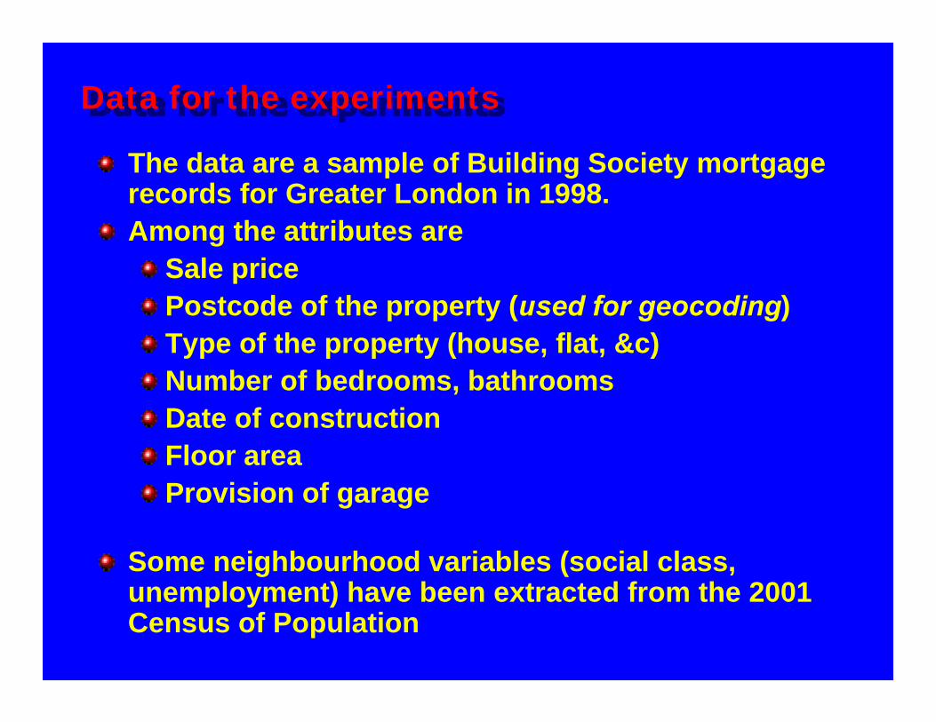
Data for the experiments

The data are a sample of Building Society mortgage records for Greater London in 1998. Among the attributes are

Sale pricePostcode of the property (used for geocoding)Type of the property (house, flat, &c)Number of bedrooms, bathroomsDate of constructionFloor areaProvision of garage

Some neighbourhood variables (social class, unemployment) have been extracted from the 2001 Census of Population

General Approach

Using the first sample as a ‘training set’ we can estimate the relationship between the sale price at location i and various X variables measured at i and the prices at nearby locations

We can then use the estimated relationship to predict the sale price for the properties in the second ‘validation’ set.

In this case we know the selling prices for the validation set, so we can compare our predictions with what happened in reality.

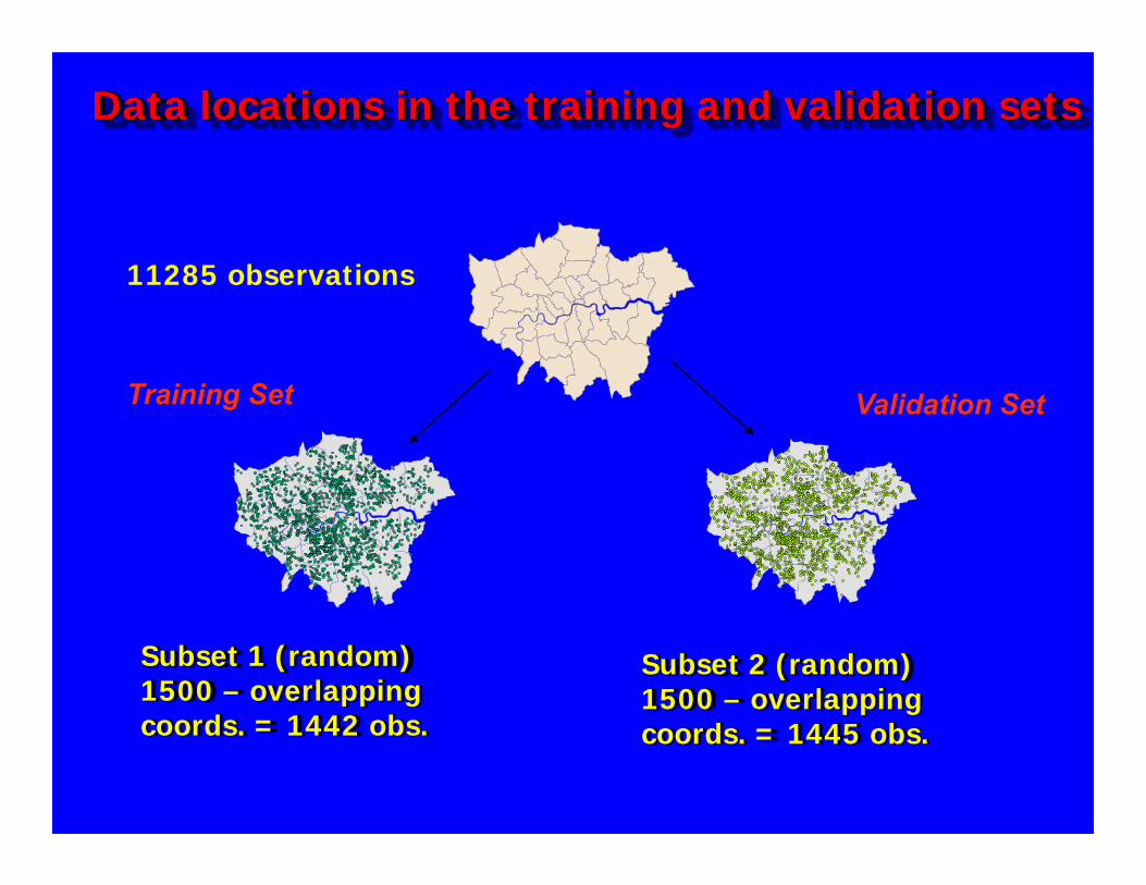
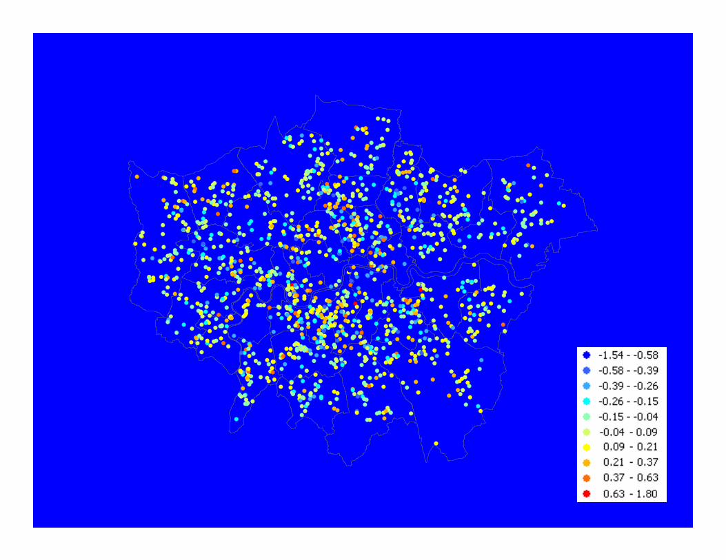
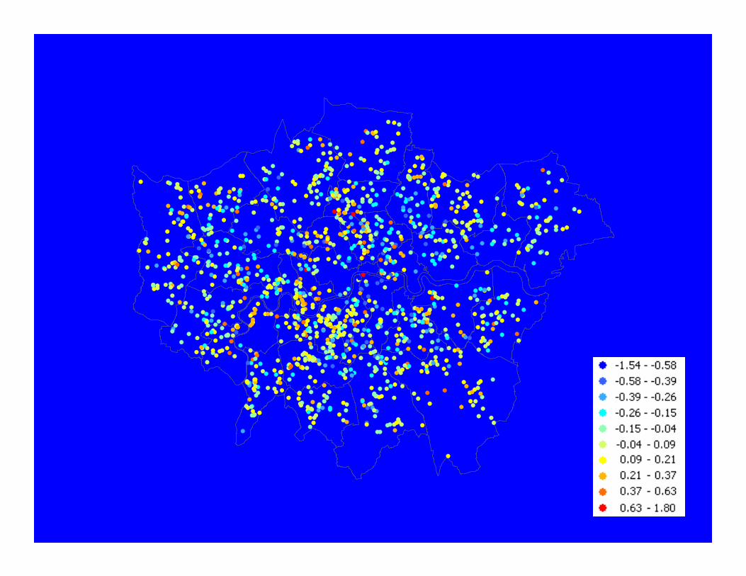
Data locations in the training and validation sets

11285 observations

Subset 1 (random)1500 – overlapping coords. = 1442 obs.

Subset 2 (random)1500 – overlapping coords. = 1445 obs.

Training Set Validation Set

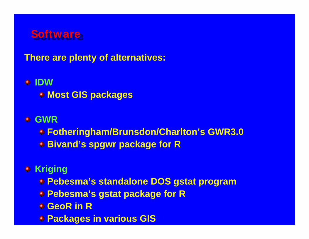
Software

There are plenty of alternatives:

IDWMost GIS packages

GWRFotheringham/Brunsdon/Charlton’s GWR3.0Bivand’s spgwr package for R

KrigingPebesma’s standalone DOS gstat programPebesma’s gstat package for RGeoR in RPackages in various GIS

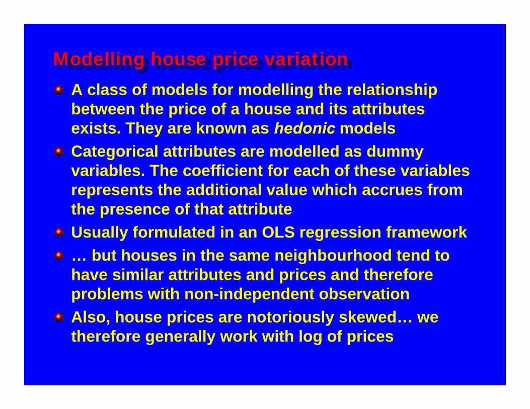
Modelling house price variationA class of models for modelling the relationship between the price of a house and its attributes exists. They are known as hedonic modelsCategorical attributes are modelled as dummy variables. The coefficient for each of these variables represents the additional value which accrues from the presence of that attributeUsually formulated in an OLS regression framework… but houses in the same neighbourhood tend to have similar attributes and prices and therefore problems with non-independent observationAlso, house prices are notoriously skewed… we therefore generally work with log of prices

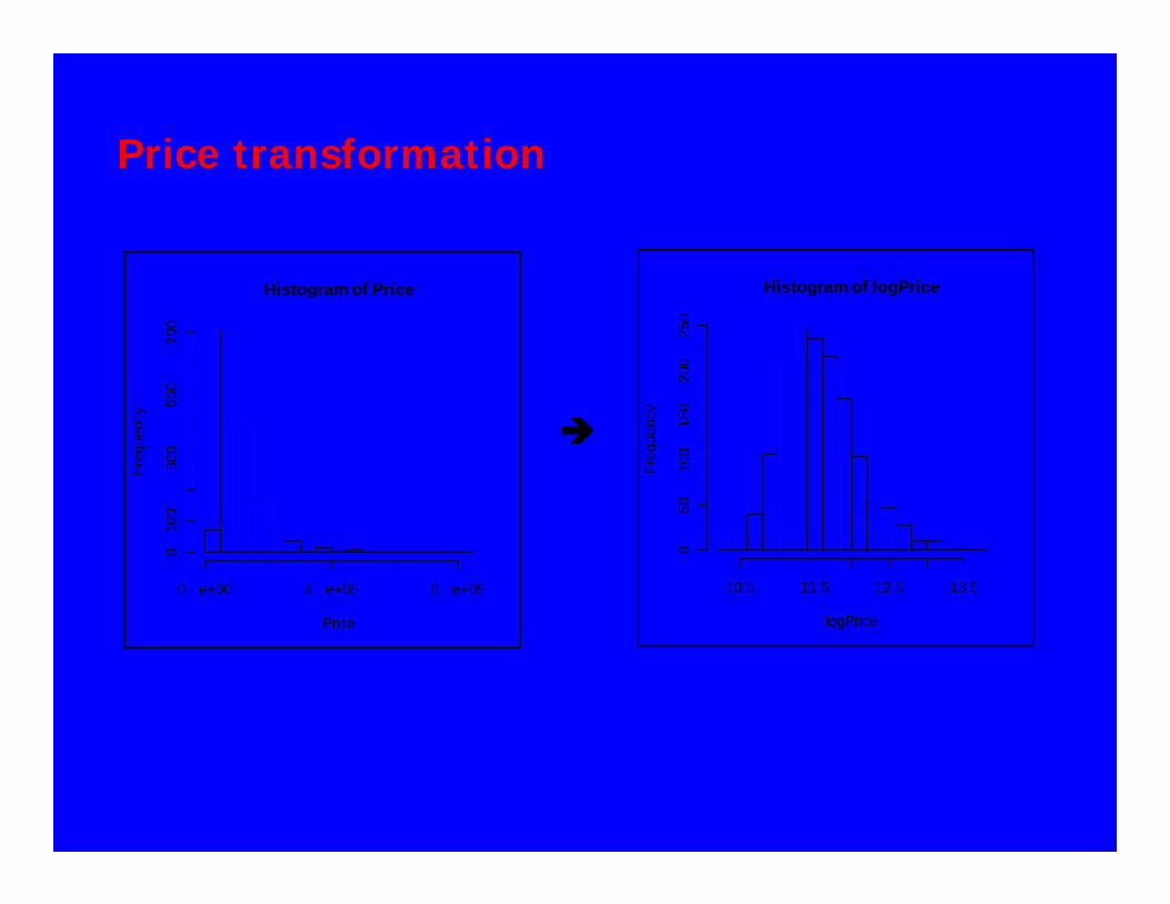
Price transformation

Logging the price variable removes the skew

Histogram of Price

Price

Freq

uenc

y

0 e+00 4 e+05 8 e+05

010

030

050

070

0

Histogram of logPrice

logPrice

Freq

uenc

y

10.5 11.5 12.5 13.5

050

100

150

200

250

Predictions based on nearby values only

1. IDW2. Ordinary Kriging

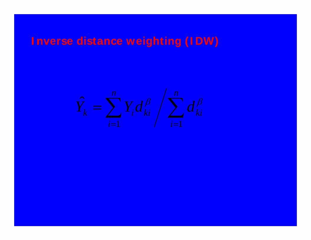
Inverse distance weighting (IDW)

∑∑==

=n

iki

n

ikiik ddYY

11

ˆ ββ

Weighted mean of Y variables. β < 0

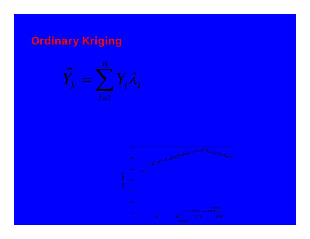
Ordinary Kriging

where ∑ λi = 1 and the weights are generated from an empirical semivariogram

∑=

=n

iiik YY

1

ˆ λ

0

0.05

0.1

0.15

0.2

0.25

0.3

0 5000 10000 15000 20000

sem

ivar

ianc

e

distance

6935

1750026123344484210048155

544815926561122625056332562830

602876001058408

Training0.025 Nug(0) + 0.225 Sph(2500)

Predictions based on nearby values and location

1.Global Regression2.Universal Kriging 3.GWR

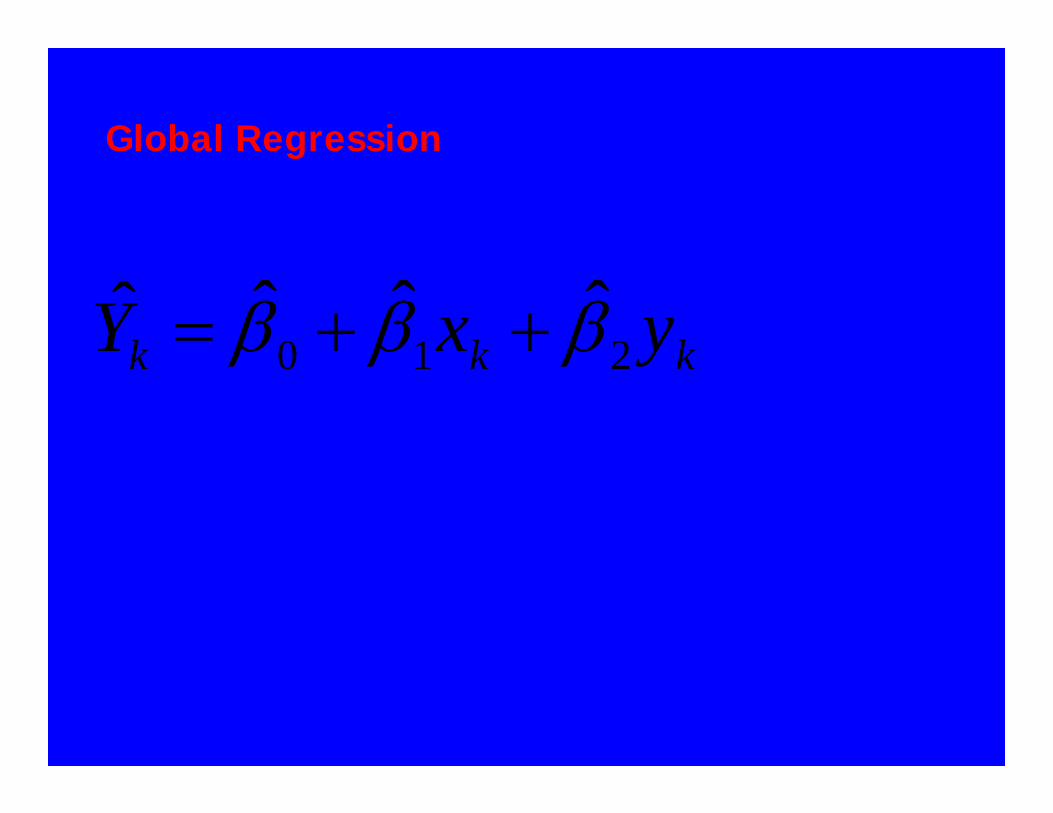
Global Regression

kkk yxY 210ˆˆˆˆ βββ ++=

where β0 is the value of Y at the origin and x,y represent the cartesian coordinates of a location.

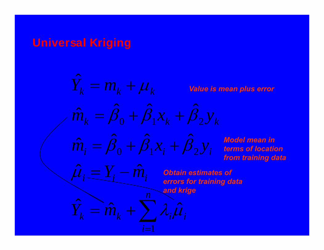
Universal Kriging

∑=

+=

−=++=

++=

+=

n

iiikk

iii

iii

kkk

kkk

mY

mYyxm

yxm

mY

1

210

210

ˆˆˆ

ˆˆ

ˆˆˆˆ

ˆˆˆˆ

ˆ

μλ

μβββ

βββ

μ Value is mean plus error

Model mean in terms of location from training data

Obtain estimates of errors for training data and krige

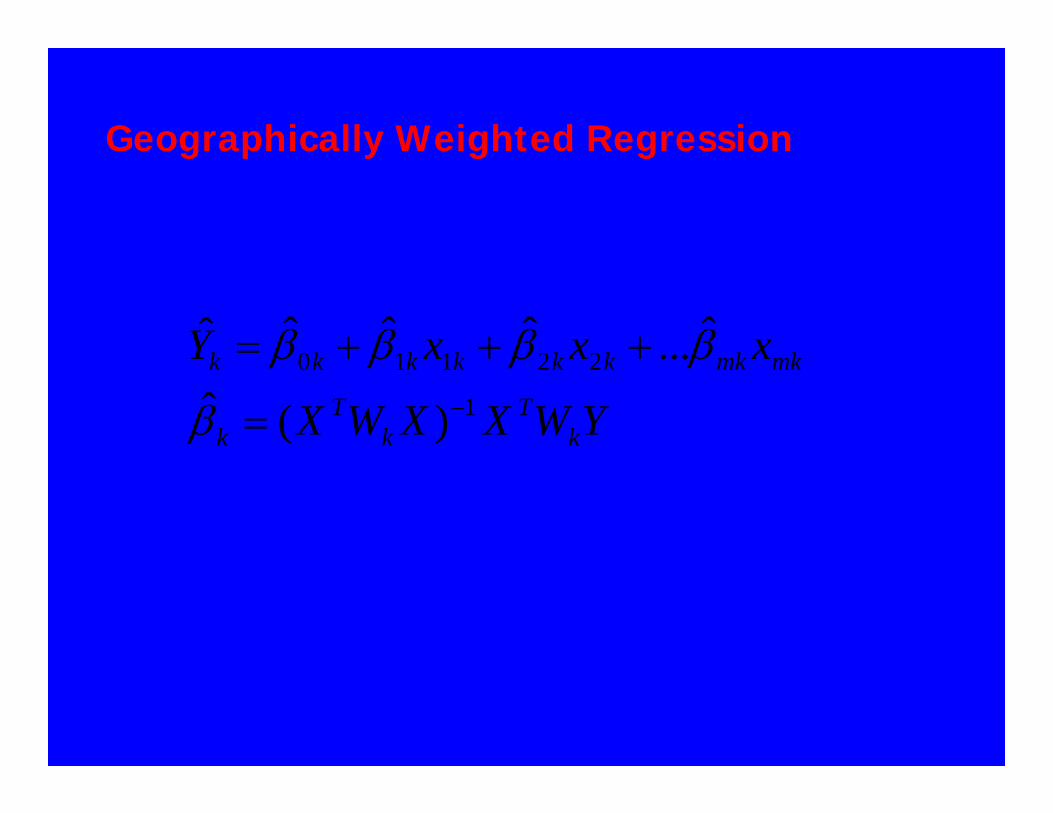
Geographically Weighted Regression

A model of spatial heterogeneity

• u is either the location of a sample point or any location in the study area (so these can be the validation point locations, or the prediction points

• Weights W(u) are generated from a kernel function which uses a bandwidth found by optimising a goodness-of-fit criterion

YWXXWX

xxxY

kT

kT

k

mkmkkkkkkk

1

22110

)(ˆ

ˆ...ˆˆˆˆ−=

+++=

β

ββββ

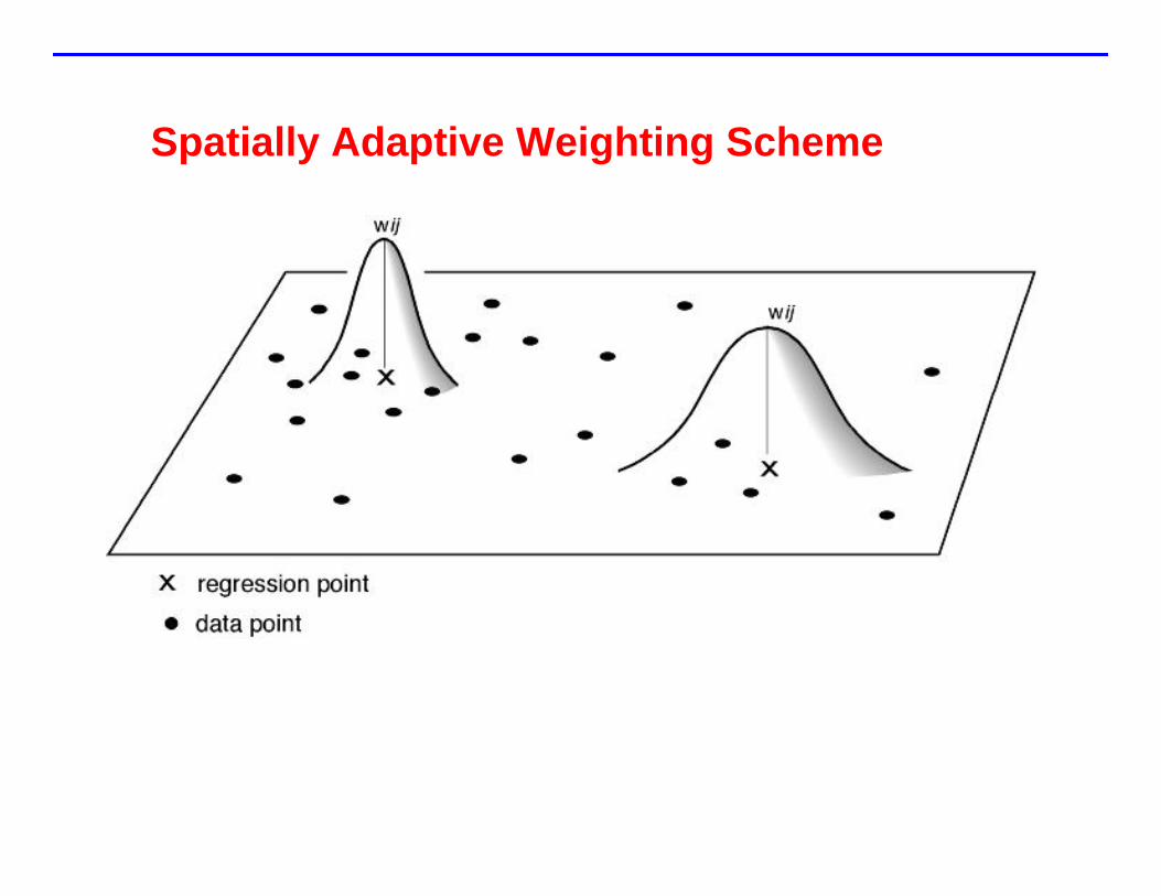
Spatially Adaptive Weighting Scheme

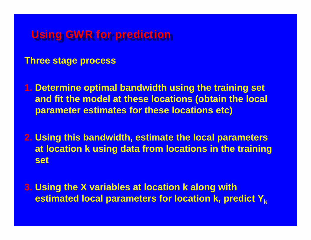
Using GWR for prediction

Three stage process

1. Determine optimal bandwidth using the training set and fit the model at these locations (obtain the local parameter estimates for these locations etc)

2. Using this bandwidth, estimate the local parameters at location k using data from locations in the training set

3. Using the X variables at location k along with estimated local parameters for location k, predict Yk

GWR outputs

Predicted dependent variable values at all locations Local parameter estimates for all locations Local standard errors for these parameter estimatesLocal T values for these parameter estimates

In addition, for the locations where Y is known (e.g. in the training set), we also get

Local influence measuresResiduals (and standardised residuals)Local goodness of fit measure (R2)Corrected Akaike Information Criterion (Hurvich/Tsai)

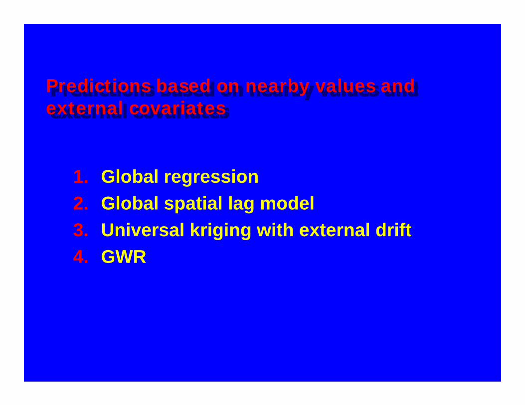
Predictions based on nearby values and external covariates

1. Global regression2. Global spatial lag model3. Universal kriging with external drift4. GWR

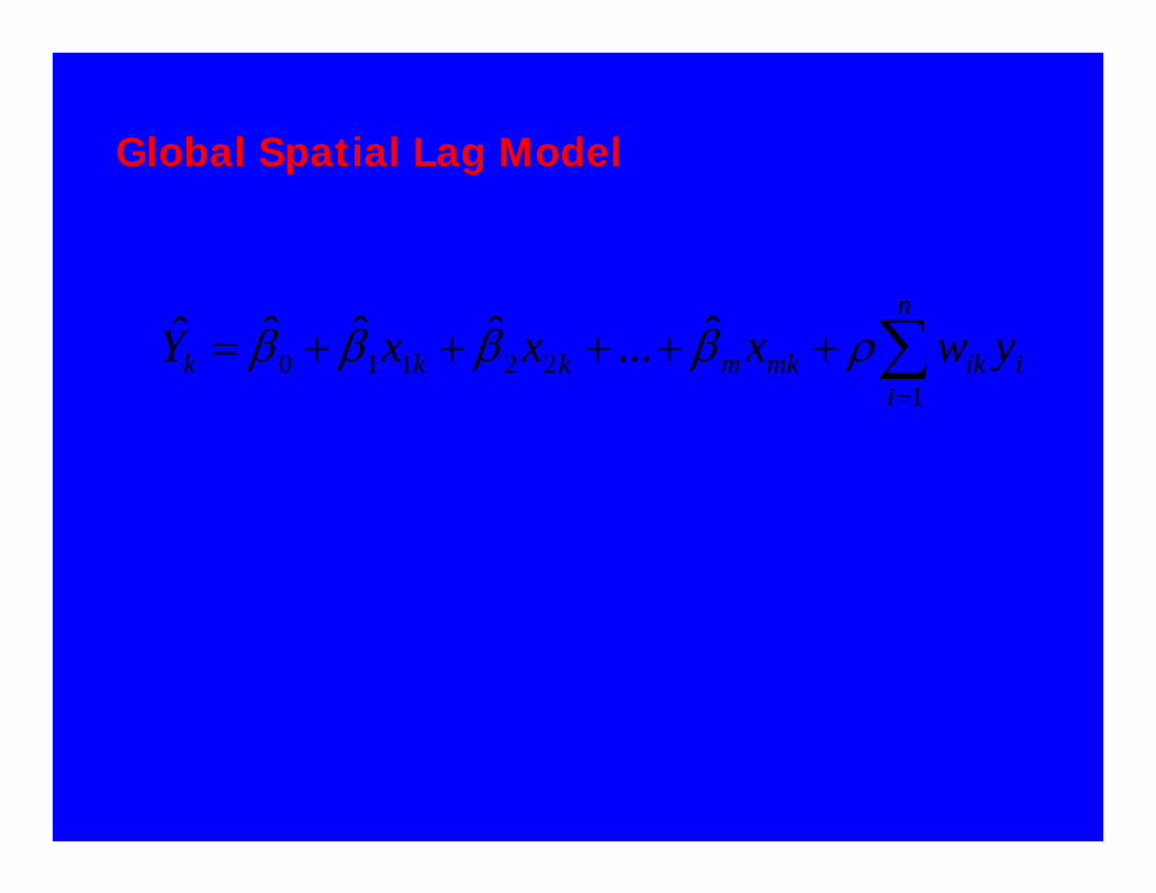
Global Spatial Lag Model

∑=

+++++=n

iiikmkmkkk ywxxxY

122110

ˆ...ˆˆˆˆ ρββββ

where ρ is a spatial autocorrelation parameter and wik is a externally derived weight for the observation at i on the regression at k

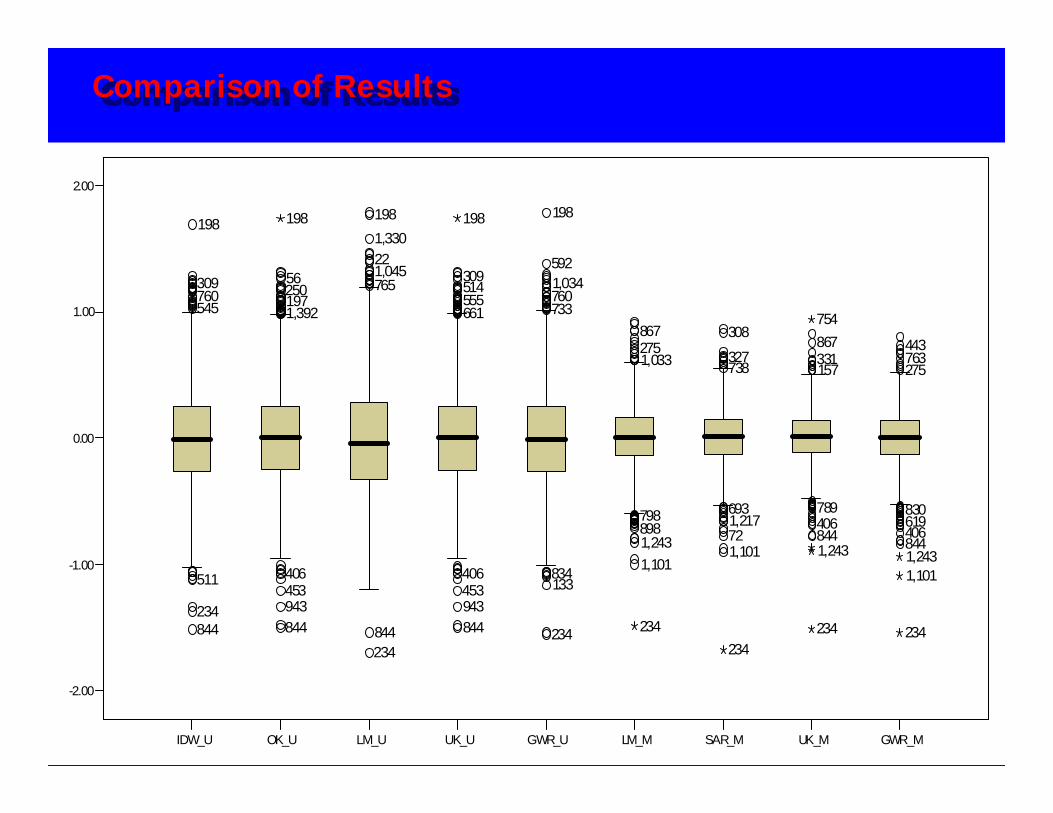
Comparison of Results

IDW_U OK_U LM_U UK_U GWR_U LM_M SAR_M UK_M GWR_M

-2.00

-1.00

0.00

1.00

2.00

844234

511

545760309

198

844943453406

1,39219725056

234844

7651,045221,330198

844943453406

661555514309

234

133834

7337601,034592

198

1,1011,243898798

1,033275867

1,101721,217693

738327

308

844406789

157331867

844406619830

275763443

198 198

234234

234

1,243

754

234

1,1011,243

Ordinary Kriging

Linear Model - locations

Universal Kriging – linear drift

Universal Kriging - hedonic

Linear Model - hedonic

GWR - hedonic

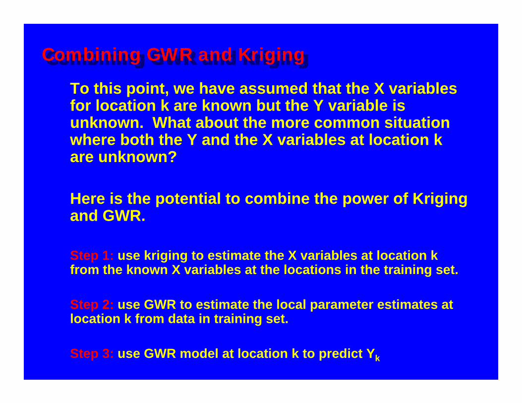
Combining GWR and Kriging

To this point, we have assumed that the X variables for location k are known but the Y variable is unknown. What about the more common situation where both the Y and the X variables at location k are unknown?

Here is the potential to combine the power of Kriging and GWR.

Step 1: use kriging to estimate the X variables at location k from the known X variables at the locations in the training set.

Step 2: use GWR to estimate the local parameter estimates at location k from data in training set.

Step 3: use GWR model at location k to predict Yk

Summary

Predicting unknown quantities at given locations is a generic spatial problemIt is neither new nor surprising that adding covariates to the prediction process is much better than simply relying on spatially weighted functions of Y or on modelling trends through spatial coordinates alone. What is perhaps surprising is the extent to which the latter two processes are still used.GWR can be used to predict values accurately (at least as well as most if not all kriging techniques) and is arguably easier to use and more intuitive in some circumstances.Combining kriging (to predict the X variables) and GWR (to obtain local parameter estimates) to predict the Y variables is the next logical step.

End of presentation

GWR Kernels

• There are several kernels which are used with GWR – the shape is not as important as the bandwidth h

• Bandwidth is chosen to minimise either a cross-validation score or an Akaike Information Criterion

• Models with different bandwidths have different hat matrices and therefore different degrees of freedom

• Bisquare kernel is frequently used

– Wi(u) = [1 - d(ui - u)2]2 if d(ui - u) < h– Wi(u) = 0 otherwise

– d(ui - u) is distance from location ui to regression point u

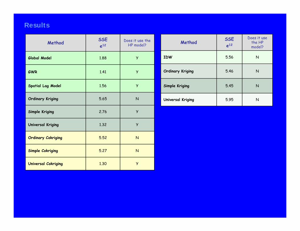
MethodSSEe12

Does it use the HP model?

Global Model 1.88 Y

GWR 1.41 Y

Spatial Lag Model 1.56 Y

Ordinary Kriging 5.65 N

Simple Kriging 2.76 Y

Universal Kriging 1.32 Y

Ordinary Cokriging 5.52 N

Simple Cokriging 5.27 N

Universal Cokriging 1.30 Y

MethodSSEe12

Does it use the HP model?

IDW 5.56 N

Ordinary Kriging 5.46 N

Simple Kriging 5.45 N

Universal Kriging 5.95 N

Results