2101

American Journal of Botany 88(11): 2101–2112. 2001.

GEOGRAPHIC DISTRIBUTION OF WILD POTATO SPECIES1

ROBERT J. HIJMANS2,4 AND DAVID M. SPOONER3

2International Potato Center, Apartado 1558, Lima 12, Peru; and3USDA, Agricultural Research Service, Department of Horticulture, University of Wisconsin, 1575 Linden Drive,

Madison, Wisconsin 53706-1590 USA

The geographic distribution of wild potatoes (Solanaceae sect. Petota) was analyzed using a database of 6073 georeferenced ob-servations. Wild potatoes occur in 16 countries, but 88% of the observations are from Argentina, Bolivia, Mexico, and Peru. Mostspecies are rare and narrowly endemic: for 77 species the largest distance between two observations of the same species is ,100 km.Peru has the highest number of species (93), followed by Bolivia (39). A grid of 50 3 50 km cells and a circular neighborhood witha radius of 50 km to assign points to grid cells was used to map species richness. High species richness occurs in northern Argentina,central Bolivia, central Ecuador, central Mexico, and south and north-central Peru. The highest number of species in a grid cell (22)occurs in southern Peru. To include all species at least once, 59 grid cells need to be selected (out of 1317 cells with observations).Wild potatoes occur between 388 N and 418 S, with more species in the southern hemisphere. Species richness is highest between 88and 208 S and around 208 N. Wild potatoes typically occur between 2000 and 4000 m altitude.

Key words: GIS; geographic distribution; geographic information systems; potato; section Petota; Solanum; Solanaceae; speciesrichness.

The wild tuber-bearing Solanum L. species (Solanaceae sect.Petota Dumort.) and outgroup relatives in Solanum sect. Etu-berosum (Bukasov and Kameraz) A. Child, hereafter calledwild potatoes, are relatives of the cultivated potato (Hawkes,1990; Contreras and Spooner, 1999). The cultivated potato(Solanum tuberosum L. and six other cultivated species thatare only grown in the Andes) is one of the world’s principalfood crops (Walker, Schmiediche, and Hijmans, 1999).

In addition to these seven cultivated potato species, thereare 199 wild potato species (Spooner and Hijmans, in press).These wild species all grow in the Americas, from the south-western United States to central Argentina and Chile. Theyhave been collected intensively to contribute to potato gene-banks, and they have been used in breeding programs to im-prove the cultivated potato (Ross, 1986; Hawkes, 1990). Thereis no evidence that wild potatoes are currently being domes-ticated or traded or that their geographic distribution is delib-erately altered by man, except for the case of S. chacoense, aspecies that is grown as an ornamental plant in Lima, Peru(Ochoa, 1962). However, in some parts of the Andes there isongoing gene flow between wild and cultivated potato species(Hawkes, 1979; Watanabe and Peloquin, 1989; Rabinowitz etal., 1990).

Despite a purported great variability in wild potatoes (Haw-kes, 1990), many of the species have a general appearancesimilar to the cultivated potato (Spooner and Van den Berg,1992). A typical wild potato has pinnately dissected leaves (afew species have entire leaves), corollas in various shades ofpurple (colors vary from white to blue to purple and pink),corollas pentagonal to rotate (some are stellate), and fruitsspherical to ovoid (some are conical). This similarity has ledto widely conflicting taxonomic treatments of wild potatoes.Hawkes (1990) and Spooner and Hijmans (2001) provide themost recent taxonomic overviews of the entire group.

1 Manuscript received 12 December 2000; revision accepted 19 April 2001.The authors thank Mariana Cruz, Jorge de la Cruz, Alberto Salas, and

Monica Tuesta for helping improve the coordinate data in the wild potatodatabase, and Luigi Guarino, Sandra Knapp, John Stares, Karl Zimmerer, andtwo unidentified reviewers for review.

4 Author for reprint requests.

Wild potatoes have been the object of intensive study. Spoo-ner and Hijmans (2001) recently reviewed wild potato system-atics and germplasm collection. Jansky (2000) reviewed thevalue of wild and cultivated potatoes in breeding for diseaseresistance. However, there has been no comprehensive analysisof the geographic distribution of wild potatoes, which we pro-vide here for the first time. We used geographic informationsystems (GIS) to analyze a large georeferenced database oflocations where wild potatoes were observed.

We computed country- and species-level statistics. For eachspecies, we estimated the geographic area over which it occursand mapped the number of observations and species richness,using grid cells. We determined the minimum number of gridcells needed to include all species and related species richnessto latitude and altitude. Species richness is used because it isa simple, widely used, well-understood, and useful measure oftaxonomic diversity (Gaston, 1996) and because it is less sen-sitive than diversity indices to the problems of unsystematicsampling intensities and procedures (Hijmans et al., 2000).

This study explores the use of geographic information sys-tems (GIS) to describe the geographic distribution of wild croprelatives. This type of study can provide baseline data for fur-ther GIS analysis for exploration, conservation, and use ofgermplasm of wild crop relatives (Guarino et al., in press), aswell as for studies of the factors that explain the geographicdistribution of these species.

MATERIALS AND METHODS

Wild potato distribution data—Our sources of wild potato distribution datawere the following: (1) the Inter-genebank Potato Database, which has datafrom seven genebanks in the USA, Peru, The Netherlands, Germany, Argen-tina, the UK, and Russia (in order of size of contribution) (Huaman, Hoekstra,and Bamberg, 2001). (2) Data from 16 collecting expeditions in 12 countriesby D. M. Spooner and coworkers (Spooner and Hijmans, 2001). These in-cluded records that are not in genebanks because they were collected as her-barium species or were lost as living specimens after collection. (3) A data-base of herbarium records developed by J. G. Hawkes (Hawkes, 1997). (4)Hawkes and Hjerting (1969; Argentina, Brazil, Paraguay and Uruguay). (5)Hawkes and Hjerting (1989; Bolivia). (6) Ochoa (1990; Bolivia). (7) Ochoa(1999, Peru). (8) Spooner et al. (1998; Guatemala). (9) Spooner et al. (1999;

2102 [Vol. 88AMERICAN JOURNAL OF BOTANY

Peru). (10) Spooner, Hoekstra, and Vilchez (2001; Costa Rica). (11) Spooneret al. (in press; Mexico).

We used all records from sources 1–3 that included a species name andpassport data. Passport data include a description of the location of origin(such as locality name), administrative units (such as departments and dis-tricts), and geographic coordinates. However, coordinate data were absent formany records. For the genebank databases, coordinates were assigned usingthe locality description where possible. For Hawkes’ (1997) database this wasonly attempted for species for which we had fewer than five observationswith coordinate data. Sources 5–7 were used to verify and improve the geo-graphic coverage of our species distribution data (see below). Additional her-barium records were taken from sources 8–11.

The presence of coordinate data allowed the analysis of the database withGIS; we used ArcView-GIS (Environmental Systems Research Institute, 1999)and DIVA-GIS software (Hijmans et al., 2001). Coordinate data in genebankdatabases often lack precision and were checked and modified following pro-cedures described by Hijmans et al. (1999). First, we checked for gross errors,such as accessions located in the oceans. Then, we made overlays (simulta-neous spatial queries) of the collection sites and administrative boundary da-tabases (first level subdivision for Mexico and Central America; first andsecond level for the United States and South America; and first, second, andthird level subdivision for Peru). We compared the names of the administrativeunits according to the wild potato distribution database with those of theadministrative boundary database. In case of discrepancies between the twodatabases, the coordinates were checked against the locality description andnew coordinates were assigned where needed.

Dot maps of the distribution of all species were compared with publishedspecies distribution maps from the floristic sources 5–7. When general areasof occurrence were already represented on our maps, we did not includeadditional points, because of a possible lack of precision of many of thesemaps, and the risk of duplicating records. However, if it appeared that ourdistribution maps did not include all major areas where a species was reportedto occur, we did copy additional observations for these areas. Species namesfollow Spooner and Hijmans (in press), who list 196 wild species in sect.Petota and three outgroup species in sect. Etuberosum. Taxonomic groupsbelow the species level (subspecies, varieties, and forms) are all treated withintheir component species.

Country- and species-level distribution—The number of observations andspecies in the database were tabulated by country. This was done separatelyfor rare species, here defined as species for which we had fewer than fiveobservations. The number of observations per species was calculated andplotted. The average number of observations per species was calculated toassess intensity of collection by country, given the species richness it harbors.

Area of distribution—For each species we estimated the area over whichit occurs, using two statistics: (1) Maximum distance (MaxD) between twoobservations of a single species was calculated as the largest distance (inmeters) between all possible pairs of observations of one species. (2) Weassigned a circular area (CAr) with a radius r to each observation and cal-culated the total area of all circles per species. Areas where circles of a speciesoverlap are only included once. Area is expressed as the area relative to thearea of one circle, i.e., the number of circular areas covered. We decided touse a radius of 50 km (i.e., CA50).

The assumption is that each point observation represents a group of plantsthat covers a circular area with a 50-km radius. Expressing CAr as the numberof circles instead of the absolute area makes it more easily comparable acrossdifferent studies and scales (when a radius other than 50 km is chosen).

The CA50 statistic was plotted against the number of observations to exploredifferences in abundance between species. A species with a relatively highnumber of observations per CA50 would be abundant within its area of dis-tribution, whereas a low number would indicate that a species was morescattered over the range in which it occurs.

To describe species distributions we use the terms ‘‘endemic’’ and ‘‘rare.’’We use ‘‘endemic’’ for species that occur in relatively small areas (have a

small range size) (Rabinowitz, 1981; Gaston and Williams, 1996) and ‘‘rare’’for species that have been observed in relatively few cases.

Grid based distribution—We compared the number of observations andspecies using a grid with 50 3 50 km cells and summarized the results bycountry. We used ArcView-GIS to transform the coordinate data to the Lam-bert equal-area azimuthal projection, with 808 W as the central meridian andthe equator as the reference latitude (Environmental Systems Research Insti-tute, 1999). Because the origin of a grid is arbitrary but can influence theresults, it may not be accurate to assign a point to one cell only, if the pointis located near one or three other cells. Therefore, the data were assigned togrid cells using a circular neighborhood (Bonham-Carter, 1994; Cressie, 1991)with a radius of 50 km, using the DIVA-GIS software. All the observationswithin that neighborhood were assigned to its respective grid cell, and anobservation can, therefore, be assigned more than once. The result is asmoother grid, which is less biased by the origin of the grid and also lesssensitive to small changes (errors) in the coordinate data. When we discussgrid cells in this paper, these refer to circles with an area of pr2 5 7854 km2

with their center in the middle of the grid cells with an area of 2500 km2.To assess the distribution of species over grid cells, we plotted the number

of species per grid cell against the number of grid cells. Data on plant dis-tributions can be biased due to spatial differences in recorder (a person whotakes data) effort (Rich and Woodruff, 1992; Gaston, 1996; Hijmans et al.,2000). In extreme cases, differences in number of species between areaswould reflect the amount of time spent there by recorders and not reflect actualdifferences in distribution. We assessed the extent to which the number ofobservations predicts the number of species by plotting the number of speciesvs. the number of observations per grid cell.

Complementarity analysis—To further analyze aspects of species distri-bution and endemicity we identified the smallest area (number of grid cells)needed to capture all wild potato species. This type of complementarity anal-ysis is typically used in studies for optimal reserve selection (Csuti et al.,1997). We used the algorithm described by Rebelo (1994; see also Rebeloand Siegfried, 1992) and implemented in the DIVA-GIS software that selectsgrid cells so as to identify the minimum set of cells that captures a maximumamount of species. The algorithm selects the cell with most species in it andthen, step by step, selects cells that contain the highest number of additional(not previously included) species. In the case of cells having the same numberof additional species, a random cell is selected from such cells. Selecting thesecomplementary cells is a nonlinear optimization problem for which Rebelo’s(1994) algorithm finds a near-optimal solution. We determined the minimumnumber of grid cells needed to include all species and mapped the locationof these grid cells.

Distribution by latitude and altitude—To summarize the species distribu-tion data, the number of species was tabulated by latitude and altitude. First,the number of species that occur in strips of 18 latitude was determined. Then,to obtain a smoothed line, for each 18 latitude zone the moving average wascalculated, using five adjacent zones (two at each side). The GTOPO30, a 300grid (each cell is ;0.8 km2) with altitude data (United States GeologicalSurvey, 1998) was used to estimate altitude for all wild potato localities. Thisestimate was only used for the records for which the passport data did notinclude altitude. Observations were then grouped in classes of 250 m altitudeand the number of species per class was plotted. The five-observation movingaverage was calculated and plotted.

RESULTS

Country- and species-level distribution—Wild potatoes oc-cur in 16 countries (Table 1). Four countries (Argentina, Peru,Bolivia, and Mexico) account for 88% of the records in thedatabase. Peru has by far the highest number of species (93species; 47% of the total). Peru also has the highest absoluteand relative (over all species in a country) number of rarespecies (here defined as species with five or fewer observa-

November 2001] 2103HIJMANS AND SPOONER—GEOGRAPHIC DISTRIBUTION OF WILD POTATOES

TABLE 1. Wild potato distribution by country. Number of observations(obs), species, rare species (obs # 5), and the ratio of observationsto species.

Country obs SpeciesRare

species obs/species

ArgentinaBoliviaBrazilChileColombiaCosta RicaEcuadorGuatemalaHondurasMexicoPanamaParaguayPeruUSAUruguayVenezuelaTotal

16881303

24100144

24142

691

9261522

1420158

1324

6073

2839

34

131

1561

3622

93323

199

450170700600

42001

72

60.333.4

8.025.011.124.0

9.511.5

1.025.7

7.511.015.352.7

6.58.0

30.5

Fig. 1. Number of observations of wild potatoes by species.

Fig. 2. Maximum distance between two observations of one wild potatospecies (MaxD) and circular area (CA50). A circular area with a 50 km radiuswas assigned to each observation. Areas where circles of a species overlapwere only counted once. The area is expressed relative to the area of onecircle. Species sequence is not necessarily the same for MaxD and CA.

tions), and 15 Peruvian species occur only once in our data-base (out of 17 species that occur once).

The distribution of the number of observations by speciesis far from uniform (Fig. 1). The most frequently observedspecies are S. acaule (630 observations), S. leptophyes (337),S. megistacrolobum (320), S. bukasovii (252), and S. cha-coense (205). These five species account for 29% of the re-cords and S. acaule alone accounts for 10%. The 72 species(36% of all species) with the least number of observations(five or less) make up only 3% of the records. A similarlyskewed distribution has been described for Bolivian genebankaccessions by Hijmans et al. (2000) and for the interpotatogenebank by Huaman, Hoekstra, and Bamberg (2001).

The ratio between the number of observations and the num-ber of species varies strongly across countries (Table 1). Theratio is very high in species-poor USA as well as in species-rich Argentina, indicating that these two countries have beenexplored more intensively for wild potatoes than have othercountries, relative to their species richness. The ratio is low inmany countries, some of which have low wild potato speciesrichness. However, other countries in this group have an in-termediate level of species richness, such as Ecuador and Co-lombia. Because the number of species tends to go up withcollecting effort, the countries with a low ratio between speciesand observations would be the most likely places to find spe-cies that have not yet been discovered.

Area of distribution—Most species are narrow endemicsand only 39 species occur in two or more countries. Most ofthese country co-occurrences are from Bolivia and Argentina(13 species in common) and from Bolivia and Peru (10 speciesin common). Solanum chacoense is the only species that oc-curs in five countries, followed by S. acaule and S. commer-sonii which occur in four countries. The average greatest dis-tance between two observations of the same species (MaxD)is 411 km. For 77 species, MaxD is ,100 km, and for 100species (50% of the total), MaxD is ,200 km (Fig. 2). Thegreatest MaxD observed was for S. acaule. At the time of thisresearch, this number had recently increased by 732 km to atotal of 3253 km, due to the recent discovery of this speciesin Ecuador (Spooner, Castillo T., and Lopez J. [1992] who

identified it as S. albicans; but Kardolus [1998] recognized itas an anomalous new hexaploid variety of S. acaule). Averagecircular area (CA50) over all species is 6.7, but its distributionis strongly skewed. Seventy-two species have a CA50 of ,2,and 124 have a CA50 of ,5 (Fig. 2).

Clearly, both maximum distance and circular area go upwith the number of observations. On average, a species has aCA50 of 0.16 times its number of observations (Fig. 3, regres-sion line). There are, however, important differences amongspecies. For example, S. acaule and S. chacoense occur in anarea of comparable size (CA50 5 73 for S. acaule and 74 forS. chacoense), but S. acaule has been observed about threetimes more often, suggesting that S. acaule is much moreabundant. Solanum commersonii is third in terms of CA50, butis only 17th in terms of number of observations. The CA50 ofS. commersonii is 0.36 times its number of observations whilefor S. acaule it is 0.12 times its number of observations. Thissuggests that S. commersonii is less abundant within its areaof distribution than S. acaule.

Grid based distribution—The grid based maps showing thenumber of observations (Fig. 4) and species richness (Fig. 5)give a much more refined picture than the country summaries

2104 [Vol. 88AMERICAN JOURNAL OF BOTANY

Fig. 3. Circular area (CA50) vs. number of observations of wild potatospecies. Each dot refers to one species. A circular area with a 50 km radiuswas assigned to each observation. Areas where circles of a species overlapwere only counted once. The area is expressed relative to the area of onecircle. Regression line: y 5 0.15x, R2 5 0.68. The two dotted lines (y 5 0.1xand y 5 0.5x) are included for comparison only.

presented in Table 1. Species richness is clearly not homoge-neously distributed within countries. There are few areas withmany species, and many areas with few species (Figs. 5, 6).The number of species follows a similar pattern to that of thenumber of observations. There is a strong positive correlationbetween the number of observations and species richness pergrid cell (Fig. 7; compare Figs. 4 and 5). On average over allgrid cells, there are 4.2 observations per species. Importantdeviations from this average are some areas in the USA andArgentina. As mentioned above, the number of observationsin these two countries is high in comparison to the number ofspecies. There is a relatively high number of samples in Ar-gentina, particularly in the areas with high diversity. For ex-ample, there are 421 observations in the cell in Argentina withthe highest number of species (17), a much higher ratio thanfor Peru (213 observations, 22 species) or Bolivia (141 ob-servations, 20 species). However, in Argentina wild potatoesoccur over a larger area than in any other country (295 gridcells) and the number of observations averaged out over thatarea has an intermediate value (17 per grid cell), lower thanthat of Peru (21) and of Bolivia (36; Table 2).

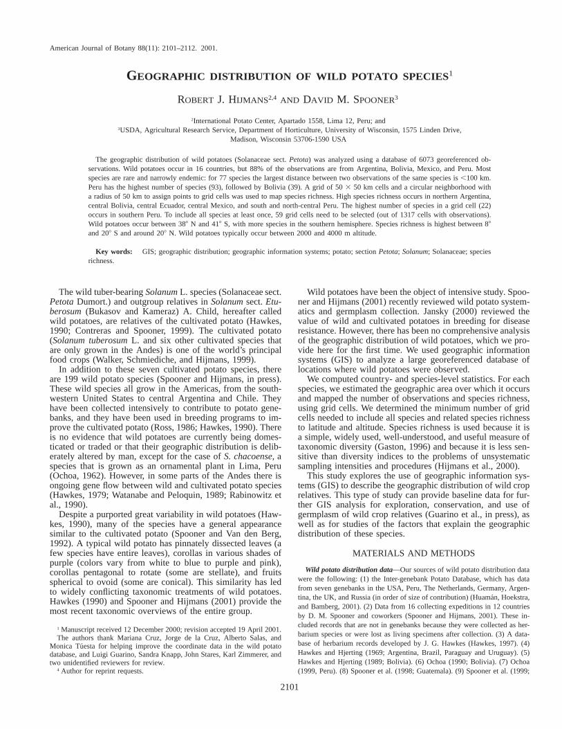
Species richness is particularly high in the southern and cen-tral Andes, and in central Mexico (Fig. 5). Going from northto south, the principal areas with high species richness are (1)the central Mexican highlands (Mexico and Michoacan states);(2) a small area in central Ecuador (Chimborazo province); (3)a stretch from northern to central Peru (in Ancash, southernCajamarca, La Libertad, and Lima departments); (4) southernPeru (in Cusco department); (5) central Bolivia (in Cochabam-ba, Chuquisaca, and Potosı and to a lesser extent La Paz anTarija departments); and (6) northern Argentina (Jujuy andSalta provinces).

There are few cells with many species (Fig. 6). Cells withmore than 15 species are only found in Peru, Bolivia, andArgentina; Ecuador and Mexico are the only two additionalcountries that have cells with nine or more species (Table 2).Only 5% of the cells have more than ten species, while 52%of the cells only have one species (Fig. 6).

The highest number of species in a single grid cell is 22

and occurs in the department of Cusco in south Peru. Twocells have 20 species, one in the Bolivian department of Potosı(on the border with Chuquisaca) and one in the Peruvian de-partment of Ancash. There are two cells in the Peruvian de-partment of Cusco with 19 species and one cell in the Boliviandepartment of Chuquisaca with 18 species. Although Peru hasmore species, its most species-rich areas are comparable inspecies richness to those of Bolivia. However, Peru has morecells with a high number of species, and its most species-richcell only has 24% of all species present in the country. Thisagain illustrates the high number of endemic species in Peru.In Bolivia, in contrast, the most species-rich grid cell has 51%of all Bolivian species (Table 2). There are also occurrencesof relatively species-rich areas in Ecuador (60% of all speciesin that country), Argentina (61%), and in all countries withonly a few species, but to a lesser extent in Colombia (31%)and Mexico (36%).

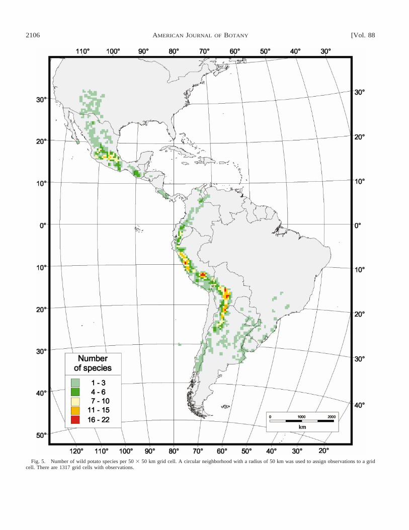
Complementarity analysis—Although nine grid cells areenough to capture 51% of all wild potato species, the mini-mum number of grid cells needed to capture all species at leastonce is 59 (out of 1317 total cells) (Figs. 8, 9). Twenty-threecells contribute only one additional species each (Fig. 9). Thelocations of the first 15 grid cells that get selected by Rebelo’s(1994) algorithm follow a pattern that can only partly be in-ferred from Fig. 5. The early appearance of cells from Mexicoand Ecuador (grid cells number 4 and 7 in Fig. 8) may seemsurprising because they have only an intermediate level of spe-cies richness (Fig. 5), but the species in these countries are alldifferent from those observed in Peru and Bolivia (the singleobservation of S. acaule mentioned above is the only excep-tion). Areas in Argentina are selected later (numbers 6 and 13in Fig. 8) than might be expected on the basis of its highnumber of species (Fig. 5). This is because some of the speciesin these cells were already included in area number 3 (Fig. 8)in southern Bolivia.

In northern Peru and southern Ecuador, there is a group offour nearby cells that are selected at an early stage (within thefirst 15 iterations). This means that in these areas, there arenot only individual cells with a high level of species richness,but that there is also a high turnover of species compositionbetween nearby grid cells. Despite its second rank (tied withEcuador) for rare species (Table 1), Colombia is not includedin the selection at an early stage because its species are notgeographically clustered (see also Fig. 5; Table 2).

Distribution by latitude and altitude—Wild potatoes occurbetween 388 N and 418 S. The highest number of species perdegree latitude (.20) occurs between 88 S and 208 S, i.e., fromnorth-central Peru to central Bolivia, and around 208 N, in thecentral Mexican highlands (Fig. 10). The distribution of thenumber of species by latitude follows a bimodal distribution.There is a remarkably similar pattern between 208 and 408 inboth hemispheres. However, in the zone between 208 N and208 S, and particularly the zones between 88 N and 158 N and88 S and 158 S, the number of species is rather different, witha conspicuously higher number of species in the southernhemisphere.

Wild potatoes are most common in the tropical highlands(compare Figs. 5 and 11), particularly between 2000 and 4000m (Fig. 12). The average elevation for all species is 2770 mwhen weighted by species, and 2890 m when giving equalweight to all observations in the database. Ninety-one percent

November 2001] 2105HIJMANS AND SPOONER—GEOGRAPHIC DISTRIBUTION OF WILD POTATOES

Fig. 4. Number of observations of wild potato species per 50 3 50 km grid cell. A circular neighborhood with a radius of 50 km was used to assignobservations to a grid cell. There are 1317 grid cells with observations.

2106 [Vol. 88AMERICAN JOURNAL OF BOTANY

Fig. 5. Number of wild potato species per 50 3 50 km grid cell. A circular neighborhood with a radius of 50 km was used to assign observations to a gridcell. There are 1317 grid cells with observations.

November 2001] 2107HIJMANS AND SPOONER—GEOGRAPHIC DISTRIBUTION OF WILD POTATOES

Fig. 6. Frequency distribution of the number of wild potato species per50 3 50 km grid cell. A circular neighborhood with a radius of 50 km wasused to assign observations to a grid cell.

Fig. 7. Ratio of the number of wild potato species to number of obser-vations for each grid cell (obs. 5 1247). Correlation coefficient 5 0.74. Re-gression line: y 5 0.11 1 1.91ln(x), R2 5 0.65.

TABLE 2. Grid-based species richness statistics by country.

Country

No. of gridcells with

one or moreobs.

Mean no.of spp. per

grid cell

Mean no.of obs. per

grid cell

Highestno. of spp.in one cell

Total no. ofspp. in thecell with

highest no. ofspp. (%)

ArgentinaBoliviaBrazilChileColombiaCosta RicaEcuadorGuatemalaHondurasMexicoPanamaParaguayPeruUSAUruguayVenezuela

295124

564965113719

2269

521

211119

2212

2.46.21.01.21.91.04.13.51.03.21.81.45.31.21.22.1

16.636.4

1.55.26.96.2

12.311.6

1.010.711.6

3.221.2

4.11.76.5

17202241961

1322

22223

6151675031

10060

10010036

1001002467

100100

of the wild potato species occur, on average, above 1750 m.Of all observations, 75% appear in areas above 2300 m. Al-most all of the lower elevation species and observations arefrom the plains and hills in Argentina, Brazil, Mexico, Para-guay, Uruguay, and USA, i.e., from high latitudes.

DISCUSSION

Although distribution maps of wild crop relatives are com-mon (e.g., Zeven and Zhukovsky, 1975), this is the first studyin which a group of closely related wild crop relatives is sys-tematically analyzed using GIS. This study is also unique inits use of a very large number of georeferenced observationsfor a single group of closely related wild species.

Wild potatoes occur between 388 N and 418 S. Species rich-ness of wild potatoes is particularly high in the Central andSouth American tropical highlands, with clear peaks between88 S and 208 S and around 208 N, i.e., areas in the Andes ofnorthern Argentina, Bolivia, Ecuador, and Peru, and in centralMexico. Peru stands out for the high number of wild potatospecies as well as for the high number of rare wild potatospecies.

Many wild potatoes species are narrowly endemic, and yeta selection of only nine grid cells was needed to include 51%of the species, which emphasizes the presence of areas of highspecies richness. In a number of countries, the most species-rich grid cell has a high percentage all species. This mightfacilitate the design of in situ conservation reserves to protectthese species (as called for by Huaman, Hoekstra, and Bam-berg, 2000). However, the clustering of species on the scaleused in this study is not directly meaningful for conservationprograms, which typically would operate in considerablysmaller areas.

The lower species richness around the equator, particularlyin the northern hemisphere, as compared with higher tropicallatitudes, contrasts with the general pattern of increasing spe-cies richness (of all flora and fauna) towards the equator (e.g.,Blackburn and Gaston, 1996; Gaston and Williams, 1996). Theabsence of cool tropical highlands appears to be an importantfactor that explains the paucity of wild potato species aroundthe equator, particularly in the northern hemisphere. The cli-mate in these equatorial areas is also more humid and less

seasonal. The absence of a clear dry (or cold) season coulddiminish the relative fitness of tuber-bearing perennials suchas wild potatoes. At higher latitudes, where the data are moresimilar for both hemispheres, there is a considerable stretch ofhigh mountains in central Mexico (the Mexican transvolcanicbelt). At even higher latitudes, wild potatoes mainly occur be-low 1500 m altitude.

Our data were gathered from several sources (expeditions)and this may have led to some redundancies. Particularly, typelocalities of rare species were visited by different expeditions,as these species may not be found elsewhere. Hence, some ofthese species are even more rare and endemic than appearsfrom our data. Overall, however, it may make our data morereliable given the timing dependency of the results of wildpotato exploration: there are differences within and amongyears in the likelihood of finding certain species in certainlocations.

Some of our records are recent, but many date back manyyears. In some cases, the habitat in which the species occurredhas now disappeared, and the species may no longer occurthere. For example, Spooner et al. (1998) describe a rapid rate

2108 [Vol. 88AMERICAN JOURNAL OF BOTANY

Fig. 8. The location of the first 15 grid cells selected and locations of the other 44 grid cells needed to include each wild potato species at least once.

November 2001] 2109HIJMANS AND SPOONER—GEOGRAPHIC DISTRIBUTION OF WILD POTATOES

Fig. 9. Number of additional species included per grid cell, when select-ing grid cells with the objective to select all species in as few grid cells aspossible. The first 15 sites correspond to the numbered grid cells in Fig. 8.

Fig. 10. Wild potato species richness by latitude. Each observation rep-resents the number of species found in a 18 latitude wide area. The line is thefive-observations moving average.

of loss of wild potato habitat in upland forests in Guatemala.However, our recent experience in Peru, and elsewhere, indi-cates that this is not always the case. For example, Spooneret al. (1999) and Salas et al. (2001) collected many wild potatospecies in Peru in the exact location, often at the type locality,where they had been collected many years before. In somecases, it was not possible to collect at documented localities,but this was often attributed to phenology, as wild potatoesoften have a short growing period. In other cases, incompletelocality data hindered collections.

Recorder effort (bias) (Rich and Woodruff, 1992; Gaston,1996; Hijmans et al., 2000) also influences the results. Nev-ertheless, the consistency of the results (there are no suddengaps in the distributions) leads us to believe that we havepresented a good representation of overall wild potato distri-bution, and this large database is one of the most comprehen-sive for any group of plants. Although the number of obser-vations per grid cell is a reasonably good predictor of thenumber of species in that cell, we do not think that a highnumber of species follows causally from a high number ofobservations.

Wild potatoes have been the object of intensive explorationover many years (Spooner and Hijmans, 2001). While therewill still be some areas where further exploration would dis-cover additional species, a low number of observations in acell is more likely to be the result than the cause of low speciesrichness. Hence, the logic might be reversed: much collectionhas taken place in areas with a known high species diversity,referred to by Hijmans et al. (2000) as ‘‘hotspot bias.’’ At-tempts could be made to correct for recorder effort throughrarefaction (estimating how many species would have beenobserved given a constant sample size per grid cell; Sanders,1968; Prendergast et al., 1993; Gaston, 1996). However, thiswould also lead to a great loss of information, because theobserved number of species would be replaced by an estimate.

Distributions of wild relatives of crop plants have previous-ly been summarized by country (e.g., Huaman, Hoekstra, andBamberg, 2001). However, countries (or their subsidiary ad-ministrative units) have different shapes and sizes. Hence, theyhave only limited value in comparing geographic distributionsof wild plants, despite the advantage of being familiar entities.Equal-area grid cells as used in this study are clearly to be

preferred. Nevertheless, there are a number of methodologicalissues that need to be considered when using grids.

Resolution (cell size) of the grid affects the results. Numberof species per grid cell will increase with the size of the gridcell, but this increase will be different among areas. We useda 50 3 50 km grid (and a circular neighborhood with a radiusof 50 km) to strike a balance between the desire for highresolution and geographic sampling bias (Hijmans et al.,2000). This bias becomes less important when grid cell sizeincreases. We used a neighborhood of 7854 km2; most otherstudies of species distribution on a continental (or global) scalehave used much larger grid cells. For example, Gaston andWilliams (1996) review various global studies using grids of611 000 km2. The same was also used by Blackburn and Gas-ton (1996) for a study on birds in the Americas. Given thehigh density of observations, it was not necessary to use suchlarge grid cells in our study. This would have amounted toserious information loss, and even smaller grid cells will bemore appropriate for design of in situ reserves or for planningcollecting expeditions to specific areas.

We used a circular neighborhood to assign values to gridcells because this gives a smoother result, particularly for areaswith few observations (Cressie, 1991; Bonham-Carter, 1994)and is less sensitive to the origin of the grid and small errorsin the locality data. However, this does include yet other fac-tors (size, shape, and method used to define the neighborhood)that need to be considered when interpreting the results, inaddition to the scale effect (effect of grid cell size). Researchis needed to better understand the effects of different griddingmethods and scales, in relation to data density and quality andthe objectives of the study.

A complication of using species richness is the existence ofconflicting taxonomic classifications (Gaston, 1996). Wild po-tatoes are a classic case in this respect (Harlan and De Wet,1971; Spooner and Van den Berg, 1992). We use the list ofspecies provided by Spooner and Hijmans (2001), which is acompilation of taxonomic names that updates Hawkes (1990).Nevertheless, future changes in species circumscription willlikely change the results presented here (Spooner and Hijmans,2001). For example, the results of ongoing research describedby Van den Berg et al. (1998) and Miller and Spooner (1999)on the 30 taxa of the S. brevicaule complex suggest a needfor reduction of the number of species in this group. Thesespecies occur in southern Peru and Bolivia and taxonomic re-vision would reduce species richness here.

2110 [Vol. 88AMERICAN JOURNAL OF BOTANY

Fig. 11. Elevation in Latin America and parts of the USA. Data source: United States Geological Survey (1998).

November 2001] 2111HIJMANS AND SPOONER—GEOGRAPHIC DISTRIBUTION OF WILD POTATOES

Fig. 12. Wild potato species richness by altitude. Each dot represents thenumber of species observed in an area covering 250 m of difference in alti-tude. The line is the five-observations (1250 m altitude difference) movingaverage.

Although Peru seems to be reasonably well explored (num-ber of species over observations), it has an extraordinarily highnumber of apparently rare species. This indicates that Perumay still harbor unknown species, as illustrated by the ten newPeruvian wild potato species described by C. M. Ochoa be-tween 1998 and 1999 (Ochoa, 1999; Spooner and Hijmans,2001). Peruvian species are also underrepresented in gene-banks, and a collecting program is currently under way to fillthis important gap (Spooner et al., 1999; Salas et al., 2001).

LITERATURE CITED

BLACKBURN, T. M., AND K. J. GASTON. 1996. Spatial patterns in the speciesrichness of birds in the New World. Ecography 19: 369–376.

BONHAM-CARTER, G. 1994. Geographic information systems for geoscien-tists. Modelling with GIS. Computer Methods in the Geosciences 13.Pergamon/Elsevier, London, UK.

CONTRERAS M. A., AND D. M. SPOONER. 1999. Revision of Solanum sectionEtuberosum (subgenus Potatoe). In M. Nee, D. E. Symon, R. N. Lester,and J. P. Jessop [eds.], Solanaceae IV, 227–245. Royal Botanic Gardens,Kew, UK.

CRESSIE, N. A. C. 1991. Statistics for spatial data. John Wiley & Sons, NewYork, New York, USA.

CSUTI, B., S. POLASKY, P. H. WILLIAMS, R. L. PRESSEY, J. D. CAMM, M.KERSHAW, A. R. KIESTER, B. DOWNS, R. HAMILTON, M. HURST, AND

K. SAHR. 1997. A comparison of reserve selection algorithms using dataon terrestrial vertebrates in Oregon. Biological Conservation 80: 83–97.

ENVIRONMENTAL SYSTEMS RESEARCH INSTITUTE. 1999. ArcView-GIS 3.1.Environmental Systems Research Institute, Redlands, California, USA.

GASTON, K. J. 1996. Species richness: measure and measurement. In K. J.Gaston [ed.], Biodiversity, a biology of numbers and difference, 77–113.Blackwell Science, London, UK.

GASTON, K. J., AND P. H. WILLIAMS. 1996. Spatial patterns in taxonomicdiversity. In K. J. Gaston [ed.], Biodiversity, a biology of numbers anddifference, 202–229. Blackwell Science, London, UK.

GUARINO, L., A. JARVIS, R. J. HIJMANS, AND N. MAXTED. In press. Geo-graphic information systems (GIS) and the conservation and use of plantgenetic resources. In: Proceedings of the international conference on sci-ence and technology for managing plant genetic diversity in the 21stcentury (SAT21), Kuala Lumpur, Malaysia, 12–16 June 2000. Interna-tional Plant Genetic Resources Institute, Rome, Italy.

HARLAN, J. R., AND J. M. J. DE WET. 1971. Towards a rational classificationof cultivated plants. Taxon 20: 509–517.

HAWKES, J. G. 1979. Evolution and polyploidy in potato species. In J. G.Hawkes, R. N. Lester, and A. D. Skelding [eds.], The biology and tax-onomy of the Solanaceae, 637–645. Academic Press, London, UK.

HAWKES, J. G. 1990. The potato: evolution, biodiversity and genetic resourc-es. Belhaven Press, London, UK.

HAWKES, J. G. 1997. A database for wild and cultivated potatoes. Euphytica93: 155–161.

HAWKES, J. G., AND J. P. HJERTING. 1969. The potatoes of Argentina, Brazil,Paraguay and Uruguay: a biosystematic study. Clarendon Press, Oxford,UK.

HAWKES, J. G., AND J. P. HJERTING. 1989. The potatoes of Bolivia, theirbreeding value and evolutionary relationships. Oxford University Press,Oxford, UK.

HIJMANS, R. J., M. CRUZ, E. ROJAS, AND L. GUARINO. 2001. DIVA-GIS,version 1.4. A geographic information system for the management andanalysis of genetic resources data. Manual. International Potato Centerand International Plant Genetic Resources Institute, Lima, Peru.

HIJMANS, R. J., K. A. GARRETT, Z. HUAMAN, D. P. ZHANG, M. SCHREUDER,AND M. BONIERBALE. 2000. Assessing the geographic representativenessof genebank collections: the case of Bolivian wild potatoes. ConservationBiology 14: 1755–1765.

HIJMANS, R. J., M. SCHREUDER, J. DE LA CRUZ, AND L. GUARINO. 1999.Using GIS to check co-ordinates of germplasm accessions. Genetic Re-sources and Crop Evolution 46: 291–296.

HUAMAN, Z., R. HOEKSTRA, AND J. B. BAMBERG. 2000. The Inter-genebankpotato database and the dimensions of wild potato germplasm. AmericanJournal of Potato Research 77: 353–362.

JANSKY, S. H. 2000. Breeding for disease resistance in potato. Plant BreedingReviews 19: 69–155.

KARDOLUS, J. P. 1998. A biosystematic analysis of Solanum acaule. Ph.D.dissertation, Wageningen Agricultural University, Wageningen, TheNetherlands.

MILLER, J. T., AND D. M. SPOONER. 1999. Collapse of species boundaries inthe Solanum brevicaule complex (Solanaceae, Sect. Petota): moleculardata. Plant Systematics and Evolution 214: 103–130.

OCHOA, C. M. 1962. Los Los Solanum tuberıferos silvestres del Peru (Tub-erarium subsecc. Hyperbasarthrum). Privately published.

OCHOA, C. M. 1990. The potatoes of South America: Bolivia. CambridgeUniversity Press, Cambridge, UK.

OCHOA, C. M. 1999. Las papas de sudamerica: Peru. International PotatoCenter, Lima, Peru.

PRENDERGAST, J. R., S. N. WOOD, J. H. LAWTON, AND B. C. EVERSHAM.1993. Correcting for variation in recording effort in analyses of diversityhotspots. Biodiversity Letters 1: 39–53.

RABINOWITZ, D. 1981. Seven forms of rarity. In H. Syne [ed.], The biologicalaspects of rare plant conservation, 205–217. John Wiley & Sons, NewYork, New York, USA.

RABINOWITZ, D., C. R. LINDER, R. ORTEGA, D. BEGAZO, H. MURGUIA, D.S. DOUCHES, AND C. F. QUIROS. 1990. High levels of interspecific hy-bridization between Solanum sparsipilum and S. stenotomum in experi-mental plots in the Andes. American Potato Journal 67: 73–81.

REBELO, A. G. 1994. Iterative selection procedures: centres of endemism andoptimal placement of reserves. Strelitzia 1: 231–257.

REBELO, A. G., AND W. R. SIEGFRIED. 1992. Where should nature reservesbe located in the Cape Floristic Region, South Africa? Models for thespatial configuration of a reserve network aimed at maximizing the pro-tection of diversity. Conservation Biology 6: 243–252.

RICH, T. C. G., AND E. R. WOODRUFF. 1992. Recording bias in botanicalsurveys. Watsonia 19: 73–75.

ROSS, H. 1986. Potato breeding: problems and perspectives. Advances inPlant Breeding 13. Paul Parey Verlag, Berlin, Germany.

SALAS A. R., D. M. SPOONER, Z. HUAMAN, R. VINCI TORRES M., R. HOEK-STRA, K. SCHULER, AND R. J. HIJMANS. 2001. Taxonomy and collectionsof wild potato species in Central and Southern Peru in 1999. AmericanJournal of Potato Research 78: 197–207.

SANDERS, H. L. 1968. Marine benthic diversity: a comparative study. Amer-ican Naturalist 102: 243–282.

SPOONER, D. M., R. CASTILLO T., AND L. LOPEZ J. 1992. Ecuador, 1991potato germplasm collecting expedition: taxonomy and new germplasmresources. Euphytica 60: 159–169.

SPOONER, D. M., AND R. J. HIJMANS. 2001. Potato systematics and germ-plasm collecting, 1989–2000. American Journal of Potato Research 78:237–268.

SPOONER, D. M., R. HOEKSTRA, R. G. VAN DEN BERG, AND V. MARTINEZ.1998. Solanum sect. Petota in Guatemala: taxonomy and genetic re-sources. American Journal of Potato Research 75: 3–17.

SPOONER, D. M., R. HOEKSTRA, AND B. VILCHEZ. 2001. Solanum sectionPetota in Costa Rica: taxonomy and genetic resources. American Journalof Potato Research 78: 91–98.

SPOONER, D. M., A. SALAS, Z. HUAMAN, AND R. J. HIJMANS. 1999. Wild

2112 [Vol. 88AMERICAN JOURNAL OF BOTANY

potato collecting expedition in southern Peru (Departments of Apurımac,Arequipa, Cusco, Moquegua, Puno, Tacna) in 1998: taxonomy and newgenetic resources. American Journal of Potato Research 76: 103–119.

SPOONER, D. M., AND R. G. VAN DEN BERG. 1992. An analysis of recenttaxonomic concepts in wild potatoes (Solanum sect. Petota). Genetic Re-sources and Crop Evolution 39: 23–37.

SPOONER, D. M., R. G. VAN DEN BERG, A. RIVERA-PENA, P. VELGUTH, A.DEL RIO, AND A. SALAS. In press. Taxonomy of Mexican and CentralAmerican members of Solanum Series Conicibaccata (sect. Petota). Sys-tematic Botany.

UNITED STATES GEOLOGICAL SURVEY. 1998. Database available at: http://edcwww.cr.usgs.gov/landdaac/gtopo30/gtopo30.html.

VAN DEN BERG, R. G., J. T. MILLER, M. L. UGARTE, J. P. KARDOLUS, J.

VILLAND, J. NIENHUIS, AND D. M. SPOONER. 1998. Collapse of mor-phological species in the wild potato Solanum brevicaule complex (So-lanaceae: sect. Petota). American Journal of Botany 85: 92–109.

WALKER, T. S., P. E. SCHMIEDICHE, AND R. J. HIJMANS. 1999. World trendsand patterns in the potato crop: an economic and geographic survey.Potato Research 42: 241–264.

WATANABE, K., AND S. J. PELOQUIN. 1989. Occurrence of 2n pollen and psgene frequencies in cultivated groups and their related wild species intuber-bearing solanums. Theoretical and Applied Genetics 78: 329–336.

ZEVEN, A. C., AND P. M. ZHUKOVSKY. 1975. Dictionary of cultivated plantsand their centres of diversity. Excluding ornamentals, forest trees andlower plants. Centre for Agricultural Publishing and Documentation (PU-DOC), Wageningen, The Netherlands.