Geoengineering impact of open ocean dissolution of olivine on atmospheric CO2, surface

ocean pH and marine biology

This article has been downloaded from IOPscience. Please scroll down to see the full text article.

2013 Environ. Res. Lett. 8 014009

(http://iopscience.iop.org/1748-9326/8/1/014009)

Download details:IP Address: 134.1.145.253The article was downloaded on 21/01/2013 at 17:02

Please note that terms and conditions apply.

View the table of contents for this issue, or go to the journal homepage for more

Home Search Collections Journals About Contact us My IOPscience

IOP PUBLISHING ENVIRONMENTAL RESEARCH LETTERS

Environ. Res. Lett. 8 (2013) 014009 (9pp) doi:10.1088/1748-9326/8/1/014009

Geoengineering impact of open oceandissolution of olivine on atmospheric CO2,surface ocean pH and marine biology

Peter Kohler, Jesse F Abrams1, Christoph Volker, Judith Hauck andDieter A Wolf-Gladrow

Alfred Wegener Institute for Polar and Marine Research (AWI), PO Box 12 01 61, D-27515Bremerhaven, Germany

E-mail: Peter.Koehler@awi.de

Received 22 October 2012Accepted for publication 7 January 2013Published 21 January 2013Online at stacks.iop.org/ERL/8/014009

AbstractOngoing global warming induced by anthropogenic emissions has opened the debate as towhether geoengineering is a ‘quick fix’ option. Here we analyse the intended and unintendedeffects of one specific geoengineering approach, which is enhanced weathering via the openocean dissolution of the silicate-containing mineral olivine. This approach would not onlyreduce atmospheric CO2 and oppose surface ocean acidification, but would also impact onmarine biology. If dissolved in the surface ocean, olivine sequesters 0.28 g carbon per g ofolivine dissolved, similar to land-based enhanced weathering. Silicic acid input, a byproductof the olivine dissolution, alters marine biology because silicate is in certain areas the limitingnutrient for diatoms. As a consequence, our model predicts a shift in phytoplankton speciescomposition towards diatoms, altering the biological carbon pumps. Enhanced olivinedissolution, both on land and in the ocean, therefore needs to be considered as oceanfertilization. From dissolution kinetics we calculate that only olivine particles with a grain sizeof the order of 1 µm sink slowly enough to enable a nearly complete dissolution. The energyconsumption for grinding to this small size might reduce the carbon sequestration efficiencyby ∼30%.

Keywords: geoengineering, carbon cycle, marine biology, olivine, enhanced weathering,ocean alkalinization, ocean fertilizationS Online supplementary data available from stacks.iop.org/ERL/8/014009/mmedia

1. Introduction

The Earth’s climate is currently perturbed by anthropogenicimpacts. The rise in atmospheric CO2 concentration causedby burning of fossil fuels and land use change leads not

Content from this work may be used under the termsof the Creative Commons Attribution-NonCommercial-

ShareAlike 3.0 licence. Any further distribution of this work must maintainattribution to the author(s) and the title of the work, journal citation and DOI.1 Present address: Leibniz-Zentrum fur Marine Tropenokologie (ZMT)GmbH, Fahrenheitstraße 6, D-28359 Bremen, Germany.

only to a global temperature increase, but also to otheradverse effects such as ocean acidification (Doney et al 2009).Over the coming century, most IPCC emission scenarios(Joshi et al 2011, Rogelj et al 2011) will lead to a globalwarming larger than 2 K, the limit that was set by theUnited Nations Framework Convention on Climate Changein Copenhagen in 2009 (UNFCCC 2009). To prevent Earth’sclimate from crossing this 2 K threshold atmospheric CO2must be stabilized below approximately 450–500 µatm.This requires massive reduction in future CO2 emissionsin the present century (Meinshausen et al 2009, Solomon

11748-9326/13/014009+09$33.00 c� 2013 IOP Publishing Ltd Printed in the UK

Environ. Res. Lett. 8 (2013) 014009 P Kohler et al

et al 2009) and even negative emissions over the nextmillennium (Friedlingstein et al 2011). In light of thesecircumstances, geoengineering is discussed as potentiallybeing of use as a relatively quick fix against these warmingtrends. Various geoengineering concepts relying on eithersolar radiation management or carbon dioxide removal (CDR)were proposed (Lenton and Vaughan 2009, The RoyalSociety 2009). CDR approaches remove CO2 from theatmosphere/surface ocean and might also address surfaceocean acidification, although some approaches re-locate theacidification problem to the seafloor (Williamson and Turley2012).

Enhanced silicate weathering—here by the dissolution ofthe silicate-containing mineral olivine—is one of the CDRapproaches. It should be mentioned that enhanced carbonateweathering (Kheshgi 1995, Caldeira and Rau 2000, Harvey2008, Rau 2008, 2011) is an alternative CDR approach whichwill not be discussed any further here. Olivine dissolution ispart of the natural silicate weathering process, which reducedatmospheric CO2 over geological timescales in the past(Berner 1990). Olivine (Mg2SiO4) is an abundantly availablemagnesium silicate which weathers according to the reaction(Schuiling and Krijgsman 2006)

(Mg, Fe)2SiO4 + 4 CO2 + 4H2O ⇒ 2(Mg, Fe)2+

+ 4 HCO−3 + H4SiO4. (1)

The abundance of Mg compared to Fe depends on the rock,but is about 90% in the well abundant dunite (Deer et al 1992).This net dissolution reaction suggests that 1 mole of olivinewould sequester 4 moles of CO2, equivalent to sequestrationrates of 0.34 g C per g olivine. It has been shown that those aretheoretical upper limits, and the effect of the ocean’s carbonchemistry lead to 20% smaller sequestration rates (Kohleret al 2010). The dissolution of one mole of olivine leads in thesurface ocean to an increase in total alkalinity by 4 moles andin silicic acid (H4SiO4) by one mole, the latter is a limitingnutrient for diatoms in large sections of the world’s oceans(Nelson et al 1995, Dugdale and Wilkerson 1998, Ragueneauet al 2006). Present day input of silicate (SiO4) due to naturalriverine fluxes (Beusen et al 2009), which account for 80%of silicate flux into the ocean (Treguer and De La Rocha2013), is 380 Tg Si yr−1 or 6 Tmol Si yr−1. The Si inputinto the ocean would be increased by 7 Tmol Si yr−1 per Pgof olivine dissolved. Recently, the geoengineering potentialof enhanced silicate weathering on land has been evaluated(Kohler et al 2010). They calculated that olivine distributedas fine powder over land areas of the humid tropics has thepotential to sequester up to 1 Pg C yr−1, but is limited by thesaturation concentration of silicic acid in rivers and streams.Here we extend the olivine dissolution scenarios from landto open ocean. We calculate for the first time not only theintended effects, but also some unintended side effects ofolivine dissolution in the open ocean on atmospheric CO2,surface ocean pH and on the marine biology with a marineecosystem model embedded in an ocean general circulationmodel. Our results also have implications for the land-basedapproach of enhanced weathering.

2. Methods

To explore the effectiveness of the enhanced weatheringof olivine, we use the biogeochemical model REcoM-2coupled to the Massachusetts Institute of Technology generalcirculation model (MITgcm). MITgcm (Marshall et al 1997)is configured globally, excluding the Arctic Ocean north of80◦N, with a longitudinal spacing of 2◦ and a latitudinalspacing that varies from 1/3◦ to 2◦, with a higher resolutionaround the equator to account for the equatorial undercurrentand to avoid nutrient trapping (Aumont et al 1999).Additionally, in the Southern Hemisphere the latitudinalresolution is scaled by the cosine of the latitude, to ensure anisotropic grid spacing even near the Antarctic continent. Themodel setup consists of 30 vertical levels, whose thicknessincreases from 10 m at the surface to 500 m in the deep ocean.A thermodynamic and dynamic sea-ice model is applied(Losch et al 2010).

The REcoM (Schartau et al 2007) (regulated ecosystemmodel) ecosystem and biogeochemistry model allows forchanges in phytoplankton C:N:Chl stoichiometry in responseto light, temperature and nutrient availability (Geider et al

1998). REcoM-2 allows for two phytoplankton speciestypes: diatoms and nanophytoplankton. The current versionof the model, and the applied forcing together with avalidation of the model’s biogeochemical fields are describedin detail elsewhere (Hauck 2012). The model structure isoutlined in figure S1 (available at stacks.iop.org/ERL/8/014009/mmedia). The model setup differs from that usedpreviously (Hauck 2012) in one detail, namely a slightlychanged parameterization of the formation of CaCO3 bynanophytoplankton. This difference leads to somewhat higheralkalinity near the surface in (Hauck 2012) than here. Themodel is spun up for a period of 100 yr from 1900 to 1999, andthen integrated from 2000 to the end of 2009 with and withoutolivine input. The period from 1900 to 1947 is forced withthe climatological CORE data set (Large and Yeager 2008).The period from 1948 to 2009 is forced with daily fields fromthe NCEP/NCAR-R1 data (Kalnay et al 1996). In the modelwe use a prescribed atmospheric CO2. Before 1958, the CO2values are derived from a spline fit (Enting et al 1994) to icecore data (Neftel et al 1985) and recent direct measurements.After 1958, annual averages of atmospheric CO2 from MaunaLoa are used (Keeling et al 2009).

We employed a non-interactive atmospheric pCO2.Neglecting the feedback of an interactive atmospheric CO2as done here may lead to an overestimation of the oceaniccarbon uptake and inventory. The reference run withoutolivine dissolution (CONTROL) is described in detail in thesupplementary data and figure S2 (available at stacks.iop.org/ERL/8/014009/mmedia). The dissolution of 1 mole of olivinewas simulated via the input of 4 moles of total alkalinity(TA) and/or 1 mole of silicic acid (Si) into the surface ocean(equation (1)). Increased alkalinity for constant dissolvedinorganic carbon leads to a reduction of the concentration ofCO2 in the surface water (Zeebe and Wolf-Gladrow 2001),followed by oceanic CO2 uptake from the atmosphere via gasexchange. We use 140 g as molar weight of olivine implying

2

Environ. Res. Lett. 8 (2013) 014009 P Kohler et al

Figure 1. Main simulation results. (a) The temporal evolution of the oceanic carbon uptake compared to CONTROL for all distributionscenarios. The short lines in year 2009 are the values for the annual mean in 2009 for scenarios STANDARD and SHIP. (b) The temporalevolution of the response of the ocean’s biology (total, diatom and non-diatom NPP, export production (of organic carbon) and of CaCO3out of the surface ocean) to olivine distribution for scenario STANDARD with respect to CONTROL. (c) Oceanic carbon uptake, total NPP,export production of organic carbon and of CaCO3 out of the surface ocean as a function of the amount of olivine dissolution (scenariosSMALL, STANDARD and LARGE with 1, 3, 10 Pg of olivine dissolution per year, respectively). Plotted are averages over the final year2009. (d) The temporal evolution of the accumulated change in mean sea surface pH.

that the dissolved olivine contains only Mg and no Fe. Thefluxes of TA and Si are evenly distributed throughout the year.We assume that olivine immediately dissolves completely, butsee section 3.2 for dissolution kinetics.

Six different olivine dissolution scenarios were simulated(table 1). The scenarios differ in (a) the amount of olivinedissolved (1, 3, 10 Pg olivine per year) to investigateany saturation/non-linear effects, (b) the input of eitherTA, or Si or both to investigate separately the effect onocean chemistry and on marine biology, and (c) the wayolivine is spatially distributed over the ocean. We distinguishbetween even distribution throughout the whole ocean and aship-based distribution. The even distribution is not a realisticscenario. Distribution via ships follows the idea of distributingdissolved olivine via ballast water of commercial ships. TheNOAA COADS (Comprehensive Ocean–Atmosphere DataSet) data set of monthly SST measurements taken by shipsof opportunity (Woodruff et al 1998) between 1959–1997 isused to serve as a proxy for ship tracks (figure S3 available atstacks.iop.org/ERL/8/014009/mmedia).

3. Results and discussion

3.1. Simulating open ocean dissolution of olivine

According to our simulation results with REcoM-2 embeddedin the MITgcm, the oceanic carbon uptake requires about

Table 1. Description of model runs.

AcronymAmount Pgolivine per year Whata

Spatial dis-tributionb

CONTROL 0 – –STANDARD 3 Si, TA EvenSTD SI 3 Si EvenSTD TA 3 TA EvenSHIP 3 Si, TA ShipSMALL 1 Si, TA EvenLARGE 10 Si, TA Even

a Distribution of silicate (Si) and/or total alkalinity (TA).b Even: over the global ocean; ship: along ship tracks.

five years to equilibrate to ∼0.29 Pg C per Pg olivine in ourSTANDARD scenario (figure 1(a)). This scenario assumes aneven distribution of 3 Pg of olivine per year over the entireopen ocean surface and calculates the effects of both alkalinityand silicic acid input. If not mentioned otherwise results referto this scenario. Our simulations show that alkalinity input isresponsible for 92%, silicic acid input for ∼8% of the carbonsequestration (figure 1(a)). Both effects are cumulative. Thecarbon sequestration caused by alkalinity is with 0.25 Pg Cper Pg olivine 10% smaller than previously assumed with asimpler model (Kohler et al 2010).

The addition of silicic acid which accompanies theolivine dissolution improves growing conditions for diatoms

3

Environ. Res. Lett. 8 (2013) 014009 P Kohler et al

Figure 2. Simulated anomalies (g C (m2 yr)−1) in scenario STANDARD with respect to CONTROL. Shown are annual average in year2009 (final year). (a) Diatom NPP. (b) Non-diatom NPP. (c) Export production of organic carbon at 87 m depth. (d) CaCO3 export at 87 mdepth.

in silicate limited waters. Our model predicts changes inthe net primary production (NPP) of diatom and non-diatomspecies groups. Diatom NPP rises by 2.4 Pg C yr−1

(+14%) to 19 Pg C yr−1, while non-diatom NPP shrinks by1.3 Pg C yr−1 (−4%) towards 32 Pg C yr−1 (figure 1(b)).Strong seasonal variations in diatom and non-diatom NPPpartially compensate each other resulting in a rather constantincrease in total NPP by 1 Pg C yr−1 (+2%) (figure 1(b)).Consequently, the species shift towards diatoms alters thebiological carbon pumps, leading to an increased exportof organic matter by about 0.08 Pg C yr−1 (+1%) and adecreased export of CaCO3 by the similar amount (−5%)(figure 1(b)). CaCO3 also has a ballasting effect on organicmatter export (De La Rocha et al 2008). A decrease of CaCO3export could therefore also lead to a decrease of carbon export,a process which is so far not considered in our study.

There is little biological response to olivine dissolutionin the Southern Ocean south of 60◦S and throughoutmost regions of the Southern Hemisphere because of thehigh natural silicate concentrations there. The diatom NPP(figure 2(a)) increases in the equatorial regime, in the coastalregime, in the North Atlantic, and in the Southern Ocean justnorth of the opal belt. The maximum increase in both totaland diatom NPP occurs in the North Atlantic where there isa low Si:N ratio and in the equatorial regime where silicateis limiting (Dugdale and Wilkerson 1998). The low latitudes

from 20◦S to 20◦N experience a fairly uniform increasein diatom NPP. Conversely, the average nanophytoplanktonNPP (figure 2(b)) was greatly reduced in the areas wherediatom NPP was increased. Spatial explicit changes in exportproduction of organic matter and CaCO3 are related to thechanges in diatom and non-diatom NPP, respectively (figures2(c) and (d)).

Olivine dissolution leads to a fairly uniform increase insea surface pH (figure S4(b) available at stacks.iop.org/ERL/8/014009/mmedia) counteracting the ongoing acidification ofthe surface ocean to some extent. Mean sea surface pH isincreased after ten years of olivine dissolution by 0.007(figure 1(d)), which is to 85% caused by the rise in alkalinityand only to the minor 15% by changes in the marine biology.Changes in carbon uptake, NPP, export production of organicmatter and CaCO3, and pH saturate after a few years (figures1(a), (b), (d)), which makes longer simulations unnecessary.The increase in oceanic carbon uptake with respect to theamount of olivine input is almost linear, with 1, 3, and 10 Pgof olivine addition leading to 0.29, 0.28, and 0.27 Pg C per Pgolivine, respectively (figure 1(c)).

In an alternative distribution scenario SHIP in whicholivine input into the surface ocean is weighted by commonship track densities (also called ships of opportunity) verysimilar results are obtained with some more localized effectson marine biology and pH. While the marine carbon uptake

4

Environ. Res. Lett. 8 (2013) 014009 P Kohler et al

Figure 3. Dissolution kinetics of olivine grains in the surface ocean. (a) Dependency of dissolution from SST (fT). Two alternativefunctions for fT are given. Global results differ by a few percentages only, mainly in cold regions (latitudes higher than 40◦). In thefollowing fT1 is used. (b) Relationship between relative dissolution rdiss and dissolution time fdiss for a given grain size of dgrain = 100 µm.(c) Calculated global mean relative dissolution rdiss as function of grain size dgrain between 0.1 and 10 µm (log x-axis). (d) Calculatedrelative dissolution rdiss for a given grain size dgrain of 1 µm as a function of maximum mixed layer depth and SST.

is with 0.28 Pg C per Pg olivine almost identical in SHIPand STANDARD (figure 1(a)), changes in marine biologyand sea surface pH are more localized in SHIP. Impacts onthe marine biology are now the results of a combinationof ship track density pattern with the spatial distribution ofsilicate limitation (figure S4 available at stacks.iop.org/ERL/8/014009/mmedia). In SHIP changes in sea surface pH arelimited to areas north of 40◦S, and they are much strongerin the Northern than in the Southern Hemisphere. In theNorth Atlantic, the impact of olivine dissolution on marinebiology is larger in SHIP than in STANDARD because moreolivine is dissolved. Marine biology in the North Pacificis not silicate limited, thus both scenarios lead to similarsmall changes in NPP and export production here. Land-basedenhanced weathering (Kohler et al 2010) would lead tosimilar effects localized to river mouths, but the amount ofsilicic acid reaching the open ocean is unknown becauseof the extensive anthropogenic alteration of the land–oceantransition (Laruelle et al 2009).

3.2. Dissolution kinetics

We calculate the grain size depending dissolution from theresidence time in the ocean surface layer and sea surfacetemperature (SST). For that purpose we generalize previous

findings (Hangx and Spiers 2009), which compiled thedependency of olivine dissolution rate as a function of grainsize and temperature. These authors assumed that olivinegrains are spherical particles, which dissolve according to ashrinking core model. Using their results we can write thefunctional dependency of dissolution time (tdiss in years),fraction of dissolution after a given time (rdiss in %), seasurface temperature (T in ◦C), and initial grain size (diameterassuming spherical shapes dgrain in µm) as

tdiss = fsize · fT · fdiss (2)fsize = dgrain/(100 µm) (3)

fT1 = e−((T−25)/10) or fT2 = 6

cosh2(T+217.5 )

(4)

fdiss = 0.023 · r2diss. (5)

Briefly, the first factor in equation (2), fsize, normalizes tothe standard case with grains of 100 µm. Previous results(Hangx and Spiers 2009) depend linearly on initial grain sizein the range from 10 to 1000 µm and we here assume itslinear extrapolation towards even smaller grain sizes. Thesecond term, fT, describes the temperature dependency. Thedissolution time (Hangx and Spiers 2009) is given for SSTof 25 ◦C (thus fT=25 ◦C = 1), tdiss roughly increases by afactor of 3 when T is reduced from 25 to 15 ◦C (figure 3(a)).

5

Environ. Res. Lett. 8 (2013) 014009 P Kohler et al

Uncertainties in dissolution are high for lower temperatures asdemonstrated by our suggested two different fitting functions(figure 3(a)). However, this effect is limited to high latitudinalareas and contributes only a few percentages to the globalrelative dissolution. In the following we will use fT1. Thethird term in equation (2), fdiss, is a second order polynomialfit to the empirically derived dependency between dissolutiontime and relative dissolution (figure 3(b)). Uncertainties on allthese functions are high, at least of the order of 50%. Thus,this exercise should only illustrate the order of magnitude inthe dissolution kinetics.

We furthermore estimate the available time for dissolu-tion tdiss from the residence time of the olivine particles inthe surface mixed layer tML. We here take the maximum ofthe monthly means of the surface mixed layer depth DMLcalculated in MITgcm, which has a global mean DML of 64 m.After Stokes law the settling velocity vStokes due to gravity canbe calculated by

vStokes = 29

· ρp − ρl

µ· g ·

�dgrain

2

�2

(6)

with the densities of the olivine particles and the waterfluid given by ρp = 3200 kg m−3 and ρl = 1000 kg m−3,respectively. The dynamic viscosity of water is µ =10−3 kg (m s)−1, g = 9.81 m s−2 is the gravitationalacceleration. We estimate the residence time tML in the surfacemixed layer as tML = DML

vStokes.

Our estimate leads to residence times of 3 yr, 10 dor 3 h for olivine particles with grain sizes of 1, 10 or100 µm, respectively. Accordingly, ∼80% of olivine in1 µm (initial diameter) grains would dissolve before leavingthe mixed layer (figure 3(d)), whereas this percentage isalready down to 5% for an initial grain size of 10 µm(figure 3(c)). Large particles will eventually dissolve inthe deep ocean and not lead to an immediate oceaniccarbon uptake. This maximum grain size estimate has alsoimplications for enhanced weathering of olivine on land.If particles are distributed on land they might potentiallybe transported by winds to open ocean areas. A previousstudy on land-based enhanced weathering (Kohler et al 2010)discussed sequestration efficiency of 10 µm large olivinegrains, a size which is easily transported by winds (Mulleret al 2010). These large grains distributed on land andpotentially dispersed by wind to the open ocean will accordingto our results sink largely undissolved to the deep oceanwithout the desired short-term carbon sequestration.

The dependences of the dissolution on both SST andmixed layer depth (figure 3(c)) also show that olivinedissolution is only feasible in the latitudinal band between40◦N and 40◦S, and additionally in the areas of deep waterproduction in the northern North Atlantic. However, theregions favourable for olivine dissolution largely overlap withcommercial shipping tracks, especially in the Atlantic (figures3(d), S3 available at stacks.iop.org/ERL/8/014009/mmedia)making a distribution scheme based on ships of opportunitiesa possible option.

Furthermore, scavenging by biogenic particles and phys-ical aggregation, especially at high particle concentrations,

might lead to larger, faster-sinking particles and aggregates.The addition of 3 Pg of olivine (as done in scenarioSTANDARD) with grain size of 1 µm homogeneouslydistributed over the world oceans would increase the numberdensity by 1011 particles per m3 in the mixed layercorresponding to 0.4 g olivine m−3. At a grain size of1 µm and below Brownian motion is the main processdriving aggregation. In a recent study (Bressac et al 2012)it was shown that adding dust particles of a similar amount(0.8 g m−3) with a somewhat smaller grain size (the numbersize distribution peaks at 0.1 µm) would lead in a part of thedistributed particles to fast particle aggregation resulting insinking velocities on the order of 50 m d−1. These velocitiesare orders of magnitude faster than our calculations implyingresidence times in the surface ocean of rather days than years.The experimental evidence (Bressac et al 2012) indicates thatour calculated sinking velocities and the estimated fractionof olivine dissolution applies only at low rates of olivineaddition.

3.3. General discussion

The sequestration of CO2 by olivine dissolution is restrictedin our study to the immediate effects caused by alkalinityenhancement and ocean fertilization by addition of silicicacid. The transition of CO2 from the atmosphere to theocean pools is thus envisaged which might play a role oncentennial to millennial timescales. On even longer timescalesapproaches which guarantee a deposition of C as part ofthe sediment on the ocean floor might need to be takeninto consideration, e.g. using calcium silicates which mightprecipitate in the form of calcite (Lackner 2002, 2003). Here,other constraints such as source material availability mightbecome important.

Our work shows that open ocean dissolution of olivineis ocean fertilization (Lampitt et al 2008). It might alsoaffect oxygen concentration below the surface if moreorganic matter is respired there. Nowadays ∼5% of theocean volume has hypoxic conditions located in the highlyproductive equatorial upwelling regions (Matear and Elliott2004, Lampitt et al 2008, Deutsch et al 2011). One study(Deutsch et al 2011) indicates that low-O2 waters are prone tofurther expansion, with the increase in anoxic water generallyconfined to intermediate waters of the equatorial Indian andPacific. The olivine dissolution leads to regionally relativelylarge impacts of up to ±30% in diatom and non-diatomNPP patterns (figures S5(a), (b) available at stacks.iop.org/ERL/8/014009/mmedia), but our simulations show less thana 10% change in regional export production of organicmatter (figures S5(c), (d) available at stacks.iop.org/ERL/8/014009/mmedia). In the upwelling regions export productionincreases by only a few per cent suggesting that the expansionof hypoxic regions due to olivine dissolution might be small.

Olivine dissolution might also lead to a substantial inputof iron into the ocean. Its impact on the marine biologymight be a subject for future studies. Back-of-the-envelopecalculations reveal that an annual dissolution of 3 Pg of olivinewith a Mg:Fe ratio of 9:1 is connected with an annual input

6

Environ. Res. Lett. 8 (2013) 014009 P Kohler et al

of 0.2 Pg Fe. This is an order of magnitude larger than thenatural iron input connected with dust deposition (Mahowaldet al 2005). Because iron solubility (and thus bio-availability)varies by several orders of magnitude between 0.01 and80% and is not well understood (Baker and Croot 2010),it is not directly clear, what the impact on marine biologywould be. Acid processing of aeolian dust particles seemsto be an important factor to enhance iron solubility interrestrial dust (Baker and Croot 2010). As this process ismissing in open ocean dissolution of olivine iron solubilityfrom these particles is expected to be on the lower endof the known range. Furthermore, other trace metals foundin olivine-containing rocks, e.g. nickel or cadmium (seegeochemistry of rocks database GEOROC, http://georoc.mpch-mainz.gwdg.de/georoc), might get dissolved and theireffects on marine ecosystems need to be considered.

The suspended olivine density of 0.4 g olivine m−3

corresponds to a flux of ∼8 g m−2 yr−1. Naturalbiogenic fluxes, e.g. our calculated export production oforganic matter (figure S2(e) available at stacks.iop.org/ERL/8/014009/mmedia) range from less than 10 to more than 200 gorganic matter m−2 yr−1 assuming a carbon content of organicmatter of 50%. This implies that especially in low-productiveopen ocean waters of the subtropical region light transparencyis expected to be reduced by the olivine input, but—as littleNPP or export production occurs there—with only marginaleffects on global biological fluxes. In high productivity areasthe relative change in the particle flux is on the order of10%. Global dust deposition in the world oceans is estimatedto about 0.5 Pg yr−1 (Mahowald et al 2005) correspondingto about 1 g m−2 yr−1, although the input is spatiallyvery heterogeneous. Furthermore, riverine input of suspendedmatter is on the order of 20 Pg yr−1 (Peucker-Ehrenbrink2009). The mass concentration of suspended particulatematter in coastal waters around Europe is in the range of 0.02to 50 g m−3 (Babin et al 2003). This implies that in coastalwaters (so-called ‘case 2’ waters) natural suspended matterconcentrations are for most cases larger than our olivine inputrates. All-together, geoengineering large scale distribution ofolivine in the open ocean surface waters might have a smallnegative effect on marine photosynthesis due to shading.

These multiple effects of olivine dissolution on themarine biology—silicic acid input, input of iron and othertrace metals, reduced water transparency—would certainlyalter our results. The addition of silicic acid added about10% to the CO2 uptake, corresponding to 0.1 Pg C yr−1 inour STANDARD scenario. The upper limit of CO2 uptakepotential for large scale iron fertilization is in the order of1 Pg C yr−1 (Aumont and Bopp 2006), but 90% of thisCO2 draw down is restricted to the Southern Ocean, whereolivine dissolution is according to our results very slow. Thecombined effect of ocean fertilization by both silicic acid andiron input was so far not investigated and might lead to somesurprising synergistic impacts.

The Lloyd’s Register Fairplay (Kaluza et al 2010)counted in year 2007 16 363 cargo ships and tankers with atotal capacity of 665×106 gross tonnage (deadweight tonnageDWT). Using an estimate for net tonnage as 50% of DWT

gives a total net tonnage of 0.33 Pg. With an average of32 ports called per ship per year this gives a total transportcapacity of 10 Pg per year. About 100 large ships (net tonnageof 300 000 t each) with a year-round commitment including32 port calls each would be necessary to distribute 1 Pg ofolivine. Alternatively, olivine might be distributed in the shipsof opportunity scenario via ballast water, which weighs atleast 30% of the DWT of ships running empty (AustralianQuarantine and Inspection Service 1993) summing up in theLloyd Register (Kaluza et al 2010) to a global ballast watercapacity of 0.2 Pg. Assuming all ships run empty every secondrun results in an annual ballast water capacity of 3.2 Pg (seealso http://globallast.imo.org/ for similar estimates), in which0.9 Pg of olivine can be dissolved considering that olivinedissolution is limited by the saturation concentration of silicicacid of 2 mmol kg−1 (Van Cappellen and Qiu 1997) derivedfrom biogenic silica reactivity. However, we like to emphasizethat the estimation of this limitation is subject to uncertainty,because direct olivine dissolution rates available to us were sofar obtained for silicic acid concentration below 1 mmol kg−1,thus at least a factor of 2 below its saturation concentration(Oelkers 2001, Pokrovsky and Schott 2000, Rimstidt et al

2012), although the decline of olivine dissolution rates forrising silicic acid concentrations (Pokrovsky and Schott 2000)hints already at a saturation effect.

Grinding particles to 1 µm grain size is a practicalchallenge which consumes by far the most energy in the wholeprocessing chain, at least an order of magnitude more thanmining and transport (Hangx and Spiers 2009, Kohler et al

2010, Renforth 2012). Energy costs for grinding 80% of theparticles down to 1 µm with present day technology are ashigh as 300–350 kWh t−1 (Renforth 2012). Depending onthe type of energy production (Rubin et al 2007) this mightrelease as much as 350 (gas) to 800 (coal) g of CO2 per kWhreducing carbon sequestration efficiency by up to 30%.

Implementation of enhanced weathering would requirean operation on a global scale that will bring olivine miningto one of the world’s largest mining sector (Schuiling andKrijgsman 2006, Mohr and Evans 2009). CO2 and othergreenhouse gases produced by grinding, mining, and transportof olivine would offset sequestration capacity of enhancedweathering. An estimate (Kohler et al 2010) assuming localmining and restricted transport (less than 1000 km and mainlyby ships) for the total CO2 expenditure is close to 10%, whichgives a carbon sequestration efficiency of 90%. This doesnot include the fuel required for ships that would distributeolivine nor the energy demand necessary for grinding tosmall grain sizes of 1 µm as calculated above. If they areincluded, carbon sequestration efficiency falls below 60% andmakes open ocean dissolution of olivine a rather inefficientgeoengineering technique.

Our results show that enhanced weathering might helpto reduce atmospheric CO2. However, with a carbon uptakerate of 0.28 g carbon per g of olivine (neglecting reducedefficiency as discussed above) the recent fossil emissionsof about 9 Pg C yr−1 (Peters et al 2012) are difficultif not impossible to be reduced solely based on olivinedissolution. An upper limit for the open ocean distribution

7

Environ. Res. Lett. 8 (2013) 014009 P Kohler et al

of olivine is difficult to estimate, but such a limit certainlydepends on shipping capacities, exploitation of olivine, andlow distribution rates to prevent particle aggregation. In ourSTANDARD scenario (3 Pg of olivine dissolution per year)about 9% of the anthropogenic CO2 emissions would becompensated. This is slightly higher than the compensationrate of about 7% after ten years of implementation for theongoing surface ocean acidification of nowadays 0.1 pH-units(Doney et al 2009).

4. Conclusions

In conclusion, our study provides a general picture of theintended and some of the unintended effects of open oceandissolution of olivine on atmospheric CO2, surface oceanpH, and marine biology. Most challenging is the necessityto grind olivine to grain sizes of the order of 1 µm toenable dissolution before sinking out of the surface mixedlayer. This size limitation is also of relevance for winddispersed olivine distributed on land. Energy consumptionfor grinding will reduce the CO2 sequestration efficiencysignificantly. It needs about 100 large dedicated ships todistribute 1 Pg of olivine per year over a large ocean surfacearea. Alternatively, the distribution of olivine in ballast waterof the fleet of commercial ships is an option which hasthe potential to distribute up to 0.9 Pg of olivine per year.Additionally, most shipping tracks lie in regions favourablefor olivine dissolution. There are two cumulative mechanismswhich contribute to the sequestration of carbon with themajority (∼92%) caused by ocean chemistry changes dueto alkalinity input and a minority (∼8%) by the changes inspecies composition and the biological carbon pumps due tosilicic acid input. Marine biology might be further influencedby the input of trace metals, e.g. Fe or Ni, and reducedlight availability connected with the olivine dissolution. Thealkalinity input counteracts the ongoing acidification of thesurface ocean. Land-based enhanced weathering of olivinemight lead to similar changes in marine biology (but morelocalized to river mouths) depending on the amount of silicicacid reaching the open ocean via rivers.

Acknowledgments

The authors declare no conflict of interest. Funding wasprovided by PACES, the research programme of AWIwithin the Helmholtz Association. JH was funded by‘Polar’ Flagship: Polar Ecosystem Change and Synthesis—PolEcoSyn, a call from the EUR-OCEANS Consortium.

References

Aumont O and Bopp L 2006 Globalizing results from ocean in situ

iron fertilization studies Glob. Biogeochem. Cycles 20 GB2017Aumont O, Orr J C, Monfray P, Madec G and Maier-Reimer E 1999

Nutrient trapping in the equatorial Pacific: the oceancirculation solution Glob. Biogeochem. Cycles 13 351–69

Australian Quarantine and Inspection Service 1993 Ballast Water

Management (Ballast Water Research Series vol 4) (Canberra:Australian Goverment Publishing Service)

Babin M, Stramski D, Ferrari G M, Claustre H, Bricaud A,Obolensky G and Hoepffner N 2003 Variations in the lightabsorption coefficients of phytoplankton, nonalgal particles,and dissolved organic matter in coastal waters around EuropeJ. Geophys. Res. 108 3211

Baker A and Croot P 2010 Atmospheric and marine controls onaerosol iron solubility in seawater Marine Chem. 120 4–13

Berner R A 1990 Atmospheric carbon dioxide levels overPhanerozoic time Science 249 1382–6

Beusen A H W, Bouwman A F, Durr H H, Dekkers A L M andHartmann J 2009 Global patterns of dissolved silica export tothe coastal zone: Results from a spatially explicit global modelGlob. Biogeochem. Cycles 23 GB0A02

Bressac M, Guieu C, Doxaran D, Bourrin F, Obolensky G andGrisoni J M 2012 A mesocosm experiment coupled withoptical measurements to assess the fate and sinking ofatmospheric particles in clear oligotrophic waters Geo-Marine

Lett. 32 153–64Caldeira K and Rau G H 2000 Accelerating carbonate dissolution to

sequester carbon dioxide in the ocean: geochemicalimplications Geophys. Res. Lett. 27 225–8

De La Rocha C L, Nowald N and Passow U 2008 Interactionsbetween diatom aggregates, minerals, particulate organiccarbon, and dissolved organic matter: further implications forthe ballast hypothesis Glob. Biogeochem. Cycles 22 GB4005

Deer W, Howie R and Zussman J 1992 An Introduction to the

Rock-Forming Minerals 2nd edn (Harlow: Longman)Deutsch C, Brix H, Ito T, Frenzel H and Thompson L 2011

Climate-forced variability of ocean hypoxia Science

333 336–9Doney S C, Fabry V J, Feely R A and Kleypas J A 2009 Ocean

acidification: the other CO2 problem Ann. Rev. Marine Sci.

1 169–92Dugdale R C and Wilkerson F P 1998 Silicate regulation of new

production in the equatorial Pacific upwelling Nature

391 270–3Enting I, Wigley T and Heimann M 1994 Future emissions and

concentrations of carbon dioxide: Key ocean/atmosphere/landanalyses Technical Report 31 (Melbourne: CSIRO Division ofAtmospheric Research)

Friedlingstein P, Solomon S, Plattner G K, Knutti R, Ciais P andRaupach M R 2011 Long-term climate implications oftwenty-first century options for carbon dioxide emissionmitigation Nature Clim. Change 1 457–61

Geider R J, MacIntyre H L and Kana T M 1998 A dynamicregulatory model of phytoplanktonic acclimation to light,nutrients, and temperature Limnol. Oceanogr. 43 679–94

Hangx S J and Spiers C J 2009 Coastal spreading of olivine tocontrol atmospheric CO2 concentrations: a critical analysis ofviability Int. J. Greenhouse Gas Control 3 757–67

Harvey L D D 2008 Mitigating the atmospheric CO2 increase andocean acidification by adding limestone powder to upwellingregions J. Geophys. Res. 113 C04028

Hauck J 2012 Processes in the Southern Ocean carbon cycle:dissolution of carbonate sediments and inter-annual variabilityof carbon fluxes PhD Thesis University of Bremen (http://hdl.handle.net/10013/epic.39964.d001)

Joshi M, Hawkins E, Sutton R, Lowe J and Frame D 2011Projections of when temperature change will exceed 2 ◦Cabove pre-industrial levels Nature Clim. Change 1 407–12

Kalnay E et al 1996 The NCEP/NCAR 40-year reanalysis projectBull. Am. Meteorol. Soc. 77 437–71

Kaluza P, Kolzsch A, Gastner M T and Blasius B 2010 Thecomplex network of global cargo ship movements J. R. Soc.

Interface 7 1093–103

8

Environ. Res. Lett. 8 (2013) 014009 P Kohler et al

Keeling R, Piper S, Bollenbacher A and Walker J 2009 AtmosphericCO2 records from sites in the SIO air sampling networkTrends: A Compendium of Data on Global Change (OakRidge, TN: Carbon Dioxide Information Analysis Center, OakRidge National Laboratory, US Department of Energy)(doi:10.3334/CDIAC/atg.035)

Kheshgi H S 1995 Sequestering atmospheric carbon dioxide byincreasing ocean alkalinity Energy 20 915–22

Kohler P, Hartmann J and Wolf-Gladrow D A 2010 Geoengineeringpotential of artificially enhanced silicate weathering of olivineProc. Natl Acad. Sci. 107 20228–33

Lackner K S 2002 Carbonate chemistry for sequestering fossilcarbon Ann. Rev. Energy Environ. 27 193–232

Lackner K S 2003 A guide to CO2 sequestration Science

300 1677–8Lampitt R et al 2008 Ocean fertilization: a potential means of

geoengineering? Phil. Trans. R. Soc. A 366 3919–45Large W and Yeager S 2008 The global climatology of an

interannually varying air-sea flux data set Clim. Dynam.

33 341–64Laruelle G G et al 2009 Anthropogenic perturbations of the silicon

cycle at the global scale: key role of the land–ocean transitionGlob. Biogeochem. Cycles 23 GB4031

Lenton T M and Vaughan N E 2009 The radiative forcing potentialof different climate geoengineering options Atmos. Chem.

Phys. 9 5539–61Losch M, Menemenlis D, Campin J M, Heimbach P and

Hill C 2010 On the formulation of sea-ice models. Part 1:effects of different solver implementations andparameterizations Ocean Model. 33 129–44

Mahowald N M, Baker A R, Bergametti G, Brooks N, Duce R A,Jickells T D, Kubilay N, Prospero J M and Tegen I 2005Atmospheric global dust cycle and iron inputs to the oceanGlob. Biogeochem. Cycles 19 GB4025

Marshall J, Adcroft A, Holl C, Perelman L and Heisey C 1997 Afinite-volume, incompressible Navier–Stokes model for studiesof the ocean on parallel computers J. Geophys. Res.

102 5753–66Matear R J and Elliott B 2004 Enhancement of oceanic uptake of

anthropogenic CO2 by macronutirent fertilization J. Geophys.

Res. 109 C04001Meinshausen M, Meinshausen N, Hare W, Raper S C B, Frieler K,

Knutti R, Frame D J and Allen M R 2009 Greenhouse-gasemission targets for limiting global warming to 2 ◦C Nature

458 1158–62Mohr S and Evans G 2009 Forecasting coal production until 2100

Fuel 88 2059–67Muller K, Lehmann S, van Pinxteren D, Gnauk T, Niedermeier N,

Wiedensohler A and Herrmann H 2010 Particlecharacterization at the Cape Verde atmospheric observatoryduring the 2007 RHaMBLe intensive Atmos. Chem. Phys.

10 2709–21Neftel A, Moor E, Oeschger H and Stauffer B 1985 Evidence from

polar ice cores for the increase in atmospheric CO2 in the pasttwo centuries Nature 315 45–7

Nelson D M, Treguer P, Brzezinski M A, Leynaert A andQueguiner B 1995 Production and dissolution of biogenicsilica in the ocean: revised global estimates, comparison withregional data and relationship to biogenic sedimentation Glob.

Biogeochem. Cycles 9 359–72Oelkers E H 2001 An experimental study of forsterite dissolution

rates as a function of temperature and aqueous Mg and Siconcentrations Chem. Geology 175 485–94

Peters G P, Marland G, Le Quere C, Boden T, Canadell J G andRaupach M R 2012 Rapid growth in CO2 emissions afterthe 2008–2009 global financial crisis Nature Clim. Change

2 2–4Peucker-Ehrenbrink B 2009 Land2Sea database of river drainage

basin sizes, annual water discharges, and suspended sedimentfluxes Geochem. Geophys. Geosyst. 10 Q06014

Pokrovsky O S and Schott J 2000 Forsterite surface composition inaqueous solutions: a combined potentiometric, electrokinetic,and spectroscopic approach Geochim. Cosmochim. Acta

64 3299–312Ragueneau O, Schultes S, Bidle K, Claquin P and Moriceau B 2006

Si and C interactions in the world ocean: importance ofecological processes and implications for the role of diatoms inthe biological pump Glob. Biogeochem. Cycles 20 GB4S02

Rau G H 2008 Electrochemical splitting of calcium carbonate toincrease solution alkalinity: implications for mitigation ofcarbon dioxide and ocean acidity Environ. Sci. Technol.

42 8935–40Rau G H 2011 CO2 mitigation via capture and chemical conversion

in seawater Environ. Sci. Technol. 45 1088–92Renforth P 2012 The potential of enhanced weathering in the UK

Int. J. Greenhouse Gas Control 10 229–43Rimstidt J D, Brantley S L and Olsen A A 2012 Systematic review

of forsterite dissolution rate data Geochim. Cosmochim. Acta

99 159–78Rogelj J, Hare W, Lowe J, van Vuuren D P, Riahi K, Matthews B,

Hanaoka T, Jiang K and Meinshausen M 2011 Emissionpathways consistent with a 2 ◦C global temperature limitNature Clim. Change 1 413–8

Rubin E S, Chen C and Rao A B 2007 Cost and performance offossil fuel power plants with CO2 capture and storage Energy

Policy 35 4444–54Schartau M, Engel A, Schroter J, Thoms S, Volker C and

Wolf-Gladrow D 2007 Modelling carbon overconsumption andthe formation of extracellular particulate organic carbonBiogeosciences 4 433–54

Schuiling R D and Krijgsman P 2006 Enhanced weathering: aneffective and cheap tool to sequester CO2 Clim. Change

74 349–54Solomon S, Plattner G K, Knutti R and Friedlingstein P 2009

Irreversible climate change due to carbon dioxide emissionsProc. Natl Acad. Sci. 106 1704–9

The Royal Society 2009 Geoengineering the Climate: Science,

Governance and Uncertainty (London: The Royal Society)(www.royalsoc.ac.uk)

Treguer P J and De La Rocha C L 2013 The world ocean silicacycle Ann. Rev. Marine Sci. 5 477–501

UNFCCC 2009 Copenhagen Accord (New York: United Nations)(http://unfccc.int/resource/docs/2009/cop15/eng/l07.pdf)

Van Cappellen P and Qiu L 1997 Biogenic silica dissolution insediments of the Southern Ocean. I. Solubility Deep Sea

Res. II: Topical Studies in Oceanography 44 1109–28Williamson P and Turley C 2012 Ocean acidification in a

geoengineering context Phil. Trans. R. Soc. A: Math., Phys.

Eng. Sci. 370 4317–42Woodruff S, Diaz H, Elms J and Worley S 1998 COADS Release 2

data and metadata enhancements for improvements of marinesurface flux fields Phys. Chem. Earth 23 517–26

Zeebe R E and Wolf-Gladrow D A 2001 CO2 in Seawater:

Equilibrium, Kinetics, Isotopes (Elsevier Oceanography Book

Series vol 65) (Amsterdam: Elsevier)

9

Supplementary Information to1

Geoengineering impact of open ocean dissolution of olivine on2

atmospheric CO2, surface ocean pH and marine biology3

P. Kohler, J.F. Abrams, C. Volker, J. Hauck, D.A. Wolf-Gladrow4

Supplementary Text: Control run5

We limit our analysis of the CONTROL run here to those variables for which we discuss the6

changes brought about by olivine input, the full model validation will be published elsewhere.7

After 100 years of spin-up important variables of the marine biology (e.g. NPP, export pro-8

duction) show some inter-annual variability that is mostly driven by the inter-annually varying9

atmospheric forcing, but no long-term trends are evident. Globally NPP is relatively constant with10

50.1 Pg C yr−1 in the final year, which is in the range of current satellite-based estimates (Carr11

et al. 2006). Diatoms account for 33% of the total NPP, while non-diatom species account for the12

other 67%. The export fluxes of organic carbon, of CaCO3 and of biogenic silica are 10.7 Pg C13

yr−1, 1.4 Pg C yr−1 and 104 Tmol Si yr−1, respectively, roughly in line with data-based estimates14

(Schlitzer 2000, Berelson et al. 2007, Treguer 2002).15

The spatial patterns of the annual average of both total and diatom NPP show maxima in16

coastal and equatorial upwelling regions, in sub-polar gyres and around the Antarctic Circumpolar17

Current (figures S2(a),(b)). In the subtropical gyres, diatom NPP is very small, while non-diatom18

NPP is more evenly distributed with a weaker maximum near the equator and a minimum in the19

Southern Ocean (figures S2(b),(c)) Except for areas with strong fresh-water influence, surface20

pH is relatively constant around 8.05, with somewhat higher values reached in the sub-polar North21

Atlantic and Pacific (figures S2(d)). Organic carbon export out of the euphotic zone is concentrated22

in the areas of highest NPP and there is very little export in the subtropical gyres (figure S2(e)).23

The carbon export production in the equatorial Pacific is likely too strong, a known feature of24

biogeochemical models with coarse resolution (Aumont et al. 1999). Export of CaCO3 is more25

homogeneous and reflects mostly the small phytoplankton NPP (figure S2(f)). Overall, the model26

gives similar spatial patterns in biological activity to other typical global biogeochemical models27

(Gehlen et al. 2006, Schneider et al. 2008, Steinacher et al. 2010).28

The net oceanic carbon uptake in the final simulated year 2009 is 1.5 Pg C yr−1. This is at29

the lower end of estimates of annual contemporary carbon uptake (Gruber et al. 2009), but it most30

1

likely also contains some contribution from the long-term adjustment of deep tracer fields, that31

have not come into equilibrium with atmospheric physical forcings yet after 110 simulated years.32

As we are focusing here mainly on differences between CONTROL and sensitivity runs, these33

effects should have only a marginal effect on our results.34

Supplementary References35

Aumont O, Orr J C, Monfray P, Madec G & Maier-Reimer E 1999 Nutrient trapping in the equa-36

torial Pacific: The ocean circulation solution Global Biogeochemical Cycles 13, 351–369.37

Berelson W M, Balch W M, Najjar R, Feely R A, Sabine C & Lee K 2007 Relating estimates of38

CaCO3 production, export, and dissolution in the water column to measurements of CaCO339

rain into sediment traps and dissolution on the sea floor: a revised global carbonate budget40

Global Biogeochemical Cycles 21, GB1024, doi: 10.1029/2006GB002803.41

Carr M E, Friedrichs M A M, Schmeltz M, Aita M N, Antoine D, Arrigo K R, Asanuma I, Aumont42

O, Barber R, Behrenfeld M, Bidigare R, Buitenhuis E T, Campbell J, Ciotti A, Dierssen43

H, Dowell M, Dunne J, Esaias W, Gentili B, Gregg W, Groom S, Hoepffner N, Ishizaka J,44

Kameda T, Le Quere C, Lohrenz S, Marra J, Melin F, Moore K, Morel A, Reddy T E, Ryan45

J, Scardi M, Smyth T, Turpie K, Tilstone G, Waters K & Yamanaka Y 2006 A comparison of46

global estimates of marine primary production from ocean color Deep-Sea Research Part II,47

Topical Studies In Oceanography 53(5-7), 741–770.48

Gehlen M, Bopp L, Emprin N, Aumont O, Heinze C & Ragueneau O 2006 Reconciling surface49

ocean productivity, export fluxes and sediment composition in a global biogeochemical ocean50

model Biogeosciences 3(4), 521–537.51

Gruber N, Gloor M, Mikaloff Fletcher S E, doney S C, Dutkiewicz S, Follows M J, Gerber M,52

Jacobson A R, Joos F, Lindsay K, Menemenlis D, Mouchet A, Muller S A, Sarmiento J L &53

Takahashi T 2009 Oceanic sources, sinks, and transport of atmospheric CO2Global Biogeo-54

chemical Cycles 23, GB1005, doi: 10.1029/2008GB003349.55

Schlitzer R 2000 Applying the adjoint method for biogeochemical modelling: export of particulate56

organic matter in the world ocean in P Kasibhatla, M Heimann, P Rayner, N Mahowald, R. G57

2

Prinn & D. E Hartley, eds, ‘Inverse methods in Global Biogeochemical Cycles’ Vol. 114 of58

Geophysical Monographs AGU Washington, D.C. pp. 107–124.59

Schneider B, Bopp L, Gehlen M, Segschneider J, Frolicher T L, Cadule P, Friedlingstein P, Doney60

S C, Behrenfeld M J & Joos F 2008 Climate-induced interannual variability of marine pri-61

mary and export production in three global coupled climate carbon cycle models Biogeo-62

sciences 5(2), 597–614.63

Steinacher M, Joos F, Frolicher T L, Bopp L, Cadule P, Cocco V, Doney S C, Gehlen M, Lindsay64

K, Moore J K, Schneider B & Segschneider J 2010 Projected 21st century decrease in marine65

productivity: a multi-model analysis Biogeosciences 7(3), 979–1005.66

Treguer P 2002 Silica and the cycle of carbon in the ocean Comptes Rendus Geoscience 334(1), 3–67

11.68

Woodruff S, Diaz H, Elms J & Worley S 1998 COADS Release 2 data and metadata enhancements69

for improvements of marine surface flux fields Physics and Chemistry of The Earth 23, 517–70

526.71

3

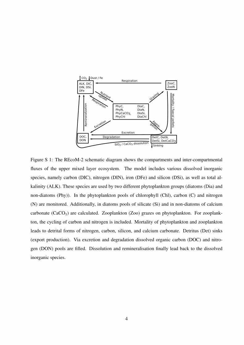
Figure S 1: The REcoM-2 schematic diagram shows the compartments and inter-compartmental

fluxes of the upper mixed layer ecosystem. The model includes various dissolved inorganic

species, namely carbon (DIC), nitrogen (DIN), iron (DFe) and silicon (DSi), as well as total al-

kalinity (ALK). These species are used by two different phytoplankton groups (diatoms (Dia) and

non-diatoms (Phy)). In the phytoplankton pools of chlorophyll (Chl), carbon (C) and nitrogen

(N) are monitored. Additionally, in diatoms pools of silicate (Si) and in non-diatoms of calcium

carbonate (CaCO3) are calculated. Zooplankton (Zoo) grazes on phytoplankton. For zooplank-

ton, the cycling of carbon and nitrogen is included. Mortality of phytoplankton and zooplankton

leads to detrital forms of nitrogen, carbon, silicon, and calcium carbonate. Detritus (Det) sinks

(export production). Via excretion and degradation dissolved organic carbon (DOC) and nitro-

gen (DON) pools are filled. Dissolution and remineralisation finally lead back to the dissolved

inorganic species.

4

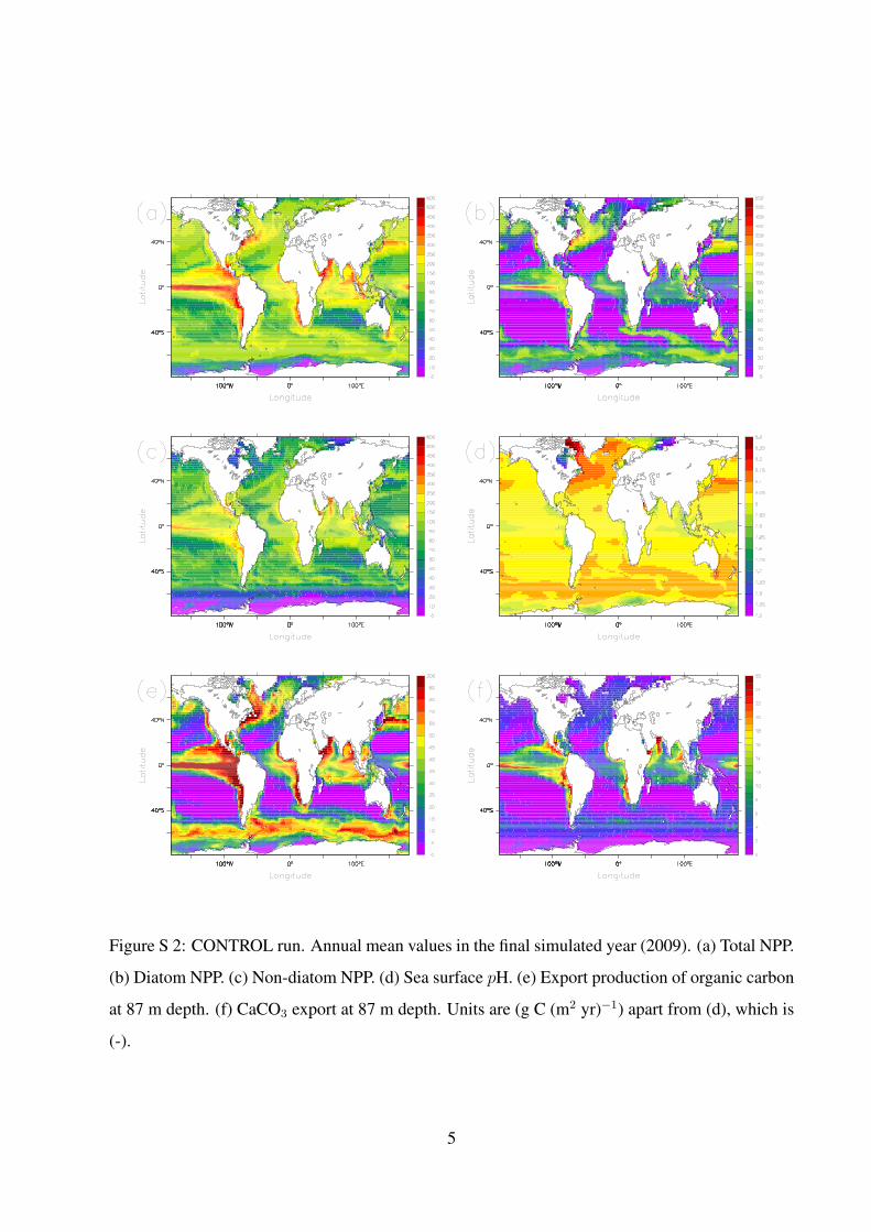
Figure S 2: CONTROL run. Annual mean values in the final simulated year (2009). (a) Total NPP.

(b) Diatom NPP. (c) Non-diatom NPP. (d) Sea surface pH. (e) Export production of organic carbon

at 87 m depth. (f) CaCO3 export at 87 m depth. Units are (g C (m2 yr)−1) apart from (d), which is

(-).

5

Figure S 3: Normalized ship track density derived from NOAA COADS data set of SST (Woodruff

et al. 1998) taken between 1959 and 1992.

6

Figure S 4: Simulated anomalies in total NPP (left) and sea surface pH (right) for scenarios STAN-

DARD and SHIP. Global surface maps of annual mean values in the final simulated year (2009).

Total NPP anomaly in (a) STANDARD vs. CONTROL and (c) SHIP vs. CONTROL. Sea surface

pH anomaly in (b) STANDARD vs. CONTROL and (d) SHIP vs. CONTROL. (e) Total NPP (SHIP

vs. STANDARD). (f) Sea surface pH (SHIP vs. STANDARD). Units in (a), (c) and (e) are (g C

(m2 yr)−1) and in (b), (d), and (f) are (-).

7

Figure S 5: Relative changes (in %) in scenario STANDARD with respect to CONTROL. Global

surface maps of annual mean values in the final simulated year (2009). (a) Non-diatom NPP, (b)

diatom NPP, (c) export production of organic matter and (d) CaCO3 export.

8