Geodesic Entropic Graphs for Dimension andEntropy Estimation in Manifold Learning

Jose A. Costa and Alfred O. Hero III

December 16, 2003

Abstract

In the manifold learning problem one seeks to discover a smooth low dimen-sional surface, i.e., a manifold embedded in a higher dimensional linear vector space,based on a set of measured sample points on the surface. In this paper we considerthe closely related problem of estimating the manifold’s intrinsic dimension and theintrinsic entropy of the sample points. Specifically, we view the sample points asrealizations of an unknown multivariate density supported on an unknown smoothmanifold. We introduce a novel geometric approach based on entropic graph meth-ods. Although the theory presented applies to this general class of graphs, we focuson the geodesic-minimal-spanning-tree (GMST) to obtaining asymptotically consis-tent estimates of the manifold dimension and the Renyi α-entropy of the sampledensity on the manifold. The GMST approach is striking in its simplicity and doesnot require reconstructing the manifold or estimating the multivariate density of thesamples. The GMST method simply constructs a minimal spanning tree (MST) se-quence using a geodesic edge matrix and uses the overall lengths of the MSTs tosimultaneously estimate manifold dimension and entropy. We illustrate the GMSTapproach on standard synthetic manifolds as well as real data sets consisting of im-ages of faces.

Keywords: Nonlinear dimensionality reduction, minimal spanning tree, intrinsic dimen-sion, intrinsic entropy, manifold learning, conformal embedding.

Corresponding author: Alfred O Hero III,Dept of EECS,Univ. of Michigan,Ann Arbor, MI 48109-2122734-763-0564 (Tel), 734-763-8041 (Fax)http://www.eecs.umich.edu/˜hero, hero@eecs.umich.edu

1

1 Introduction

Consider a class of natural occurring signals, e.g., recorded speech, audio, images, or

videos. Such signals typically have high extrinsic dimension, e.g., as characterized by the

number of pixels in an image or the number of time samples in an audio waveform. How-

ever, most natural signals have smooth and regular structure, e.g. piecewise smoothness,

that permits substantial dimension reduction with little or no loss of content information.

For support of this fact one needs only consider the success of image, video and audio

compression algorithms, e.g. MP3, JPEG and MPEG, or the widespread use of efficient

computational geometry methods for rendering smooth three dimensional shapes.

A useful representation of a regular signal class is to model it as a set of vectors which

are constrained to a smooth low dimensional manifold embedded in a high dimensional

vector space. This manifold may in some cases be a linear, i.e., Euclidean, subspace but

in general it is a non-linear curved surface. A problem of substantial recent interest in

machine learning, computer vision, signal processing and statistics is the determination

of the so-calledintrinsic dimensionof the manifold and the reconstruction of the manifold

from a set of samples from the signal class [17,26–28,34,36,37]. This problem falls in the

area ofmanifold learningwhich is concerned with discovering low dimensional structure

in high dimensional data.

When the samples are drawn from a large population of signals one can interpret

them as realizations from a multivariate distribution supported on the manifold. As this

distribution is singular in the higher dimensional embedding space it has zero entropy as

defined by the standard Lebesgue integral over the embedding space. However, when

defined as a Lebesgue integral restricted to the lower dimensional manifold the entropy

can be finite. This finiteintrinsic entropycan be useful for exploring data compression

over the manifold or, as suggested in [22], clustering of multiple sub-populations on the

manifold. The question that we address in this paper is: how to simultaneously estimate

2

the intrinsic dimension and intrinsic entropy on the manifold given a set of random sample

points? We present a novel geometric probability approach to this question which is based

on entropic graph methods developed by us and reported in publications [20–22].

Techniques for manifold learning can be classified into three categories: linear meth-

ods, local methods, and global methods. Linear methods include principal components

analysis (PCA) [25] and classical multidimensional scaling (MDS) [13]. They are based

on analyzing eigenstructure of empirical covariance matrices, and can be reliably ap-

plied only when the manifold is a linear subspace. Local methods include linear local

imbedding (LLE) [34], locally linear projections (LLP) [24], Laplacian eigenmaps [4],

and Hessian eigenmaps [17]. They are based on local approximation of the geometry of

the manifold, and are computationally simple to implement. Global approaches include

ISOMAP [36] and C-ISOMAP [15]. They preserve the manifold geometry at all scales,

and have better stability than local methods when the number of manifold samples is

limited.

With regards to estimation of the intrinsic dimensionm several methods have been

proposed [25, 33]. Most of these methods are based on linear projection techniques: a

linear map is explicitly constructed and dimension is estimated by applying Principal

Component Analysis (PCA), factor analysis, or MDS to analyze the eigenstructure of the

data. These methods rely on the assumption that only a small number of the eigenvalues of

the (processed) data covariance will be significant. Linear methods tend to overestimatem

as they don’t account for non-linearities in the data. Both nonlinear PCA [27] methods and

the ISOMAP circumvent this problem but they still rely on possibly unreliable and costly

eigenstructure estimates. Other methods have been proposed based on local geometric

techniques, e.g., estimation of local neighborhoods [37] or fractal dimension [8], and

estimating packing numbers [26] of the manifold.

We propose a geodesic-minimal-spanning-tree (GMST) method that jointly esti-

mates both the intrinsic dimension and intrinsic entropy on the manifold. The method

3

is implemented as follows. First a complete geodesic graph between all pairs of data sam-

ples is constructed, as in ISOMAP or C-ISOMAP. Then a minimal spanning graph, the

GMST, is obtained by pruning the complete geodesic graph down to a subgraph that still

connects all points but has minimum total geodesic length. The intrinsic dimension and

intrinsic α-entropy are then estimated from the GMST length functional using a simple

linear least squares (LLS) and method of moments (MOM) procedure.

The GMST method falls in the category of global approaches to manifold learn-

ing but it differs significantly from the aforementioned methods. First, it has a different

scope. Indeed, unlike ISOMAP and C-ISOMAP, the GMST method provides a statisti-

cally consistent estimate of the intrinsic entropy in addition to the intrinsic dimension of

the manifold. To the best of our knowledge no other such technique has been proposed

for learning manifold dimension. Second, unlike local methods that work on chunks of

data in local neighborhoods, GMST works on resampled data distributed over the global

data set. Third, the GMST method is simple and elegant: it estimates intrinsic entropy

and dimension by detecting the rate of increase of a GMST as a function of the number

of its resampled vertices.

The aims of this paper are limited to introducing GMST as a novel method for esti-

mating manifold dimension and entropy of the samples. As in work of others on dimen-

sion estimation [8,26] we do not here consider the issue of reconstruction of the complete

manifold. Similarly to these authors, we believe that dimension estimation and entropy

estimation for non-linear data are of interest in their own right. We also do not consider

the effect of additive noise or outliers on the performance of GMST. Finally, the consis-

tency results of GMST reported here are limited to domain manifolds defined by some

smooth unknown mapping. The extension of GMST methodology to general target man-

ifolds, e.g. those defined by implicit level set embeddings [29, 30], is a worthwhile topic

for future investigation.

What follows is a brief outline of the paper. We review some necessary background

4

on the mathematics of domain manifolds in Sec. 2. In Sec. 3 we review the asymptotic

theory of entropic graphs and obtain several new results required for their extension to

embedded manifolds. In Sec. 4 we define the general GMST algorithm. Finally, in Sec.

5 we test the GMST algorithm on standard synthetic manifolds and on a real data set

consisting of human faces from different subjects.

2 Geometric Background

2.1 A 3D Example

To illustrate ideas consider a 2D surface embedded in 3D Euclidean space, called the

embedding space. Letx1,x2, . . . ⊂ U ⊆ R2 be a set of points (samples) in a subset

U of the plane. Naturally, the shortest path between any pair(xi,xj) of these points is

given by the straight line inR2 connecting them, with corresponding distance given by

its Euclidean (L2) length,|xi − xj|. Now let U be used as a parameterization space to

describe a curved surface inR3 via a mappingϕ : U → R3. SurfacesM = ϕ(U) defined

in this explicit manner are called domain or parameterized manifolds and they inherit the

topological dimension, equal to 2 in this case, of the parameterization space. Whenϕ

is non-linear, the shortest path onM between pointsyi = ϕ(xi) andyj = ϕ(xj) is a

curve on the surface called the geodesic curve. In this paper we will primarily consider

domain manifolds defined by conformal mappingsϕ. Such conformal embeddings have

the property that the angles between tangent vectors to the surface are identical to angles

between corresponding vectors in the parameterization space, possibly up to a smoothly

varying local scale factor. This property guarantees that, regardless of how the mapping

ϕ “deforms”U ontoM, the geodesic distances inM are closely related to the Euclidean

distances inU . When this smooth surface representation holds there exist algorithms,

e.g. ISOMAP and C-ISOMAP [15, 36], which can be used to estimate the Euclidean

distances between points inU from estimates of the geodesic distances between points in

5

M. If a certain type of minimal spanning graph is constructed using these estimates, well

established results in geometrical probability [22,38] allow us to develop simple estimates

of both entropy and dimension of the points distributed on the surface.

2.2 Differential Geometry Setting

In the following, we recall some facts from differential geometry needed to formalize and

generalize the ideas just described. We will consider smooth manifolds embedded inRd.

For the general theory we refer the reader to any standard book in differential geometry

(for example, [9], [10], [7]). Anm-dimensionalsmooth manifoldM ⊆ Rd is a set such

that each of its points has a neighborhood that can be parameterized by an open set of

Rm through a local change of coordinates. Intuitively, this means that althoughM is a

(hyper) surface inRd, it can be locally identified withRm.

Let ϕ : Ω 7→ M be a mapping between two manifolds,Ω,M. Let γ be a curve

in Ω. The tangent mapdϕx assigns each tangent vectorv to Ω at pointx the tangent

vectordϕxv to M at pointϕ(x), such that, ifv is the initial velocity ofγ in Ω, then

dϕxv is the initial velocity of the curveϕ(γ) in M. For example, ifx ∈ U ⊆ Ω ⊆ Rm,

with U an open set ofRm, thendϕxv = Jϕ(x) v, whereJϕ = [∂ϕi/∂xj], i = 1, . . . , d,

j = 1, . . . ,m, is the Jacobian matrix associated withϕ at pointx ∈ Ω.

The lengthof a smooth curveΓ : [0, 1] → M is defined as(Γ) =∫ 1

0| ddt

Γ(t)|dt.

Thegeodesic distancebetween pointsy0,y1 ∈M is the length of the shortest (piecewise)

smooth curve between the two points:

dM(y0,y1) = infΓ`(Γ) : Γ(0) = y0, Γ(1) = y1 .

We can now define the following types of embeddings.

Definition 1 ϕ : Ω 7→ M is called a conformal mapping ifϕ is a diffeomorphism (i.e.,

ϕ is differentiable, bijective with differentiable inverseϕ−1) and, at each pointx ∈ Ω, ϕ

6

preserves the angles between tangent vectors, i.e.,

(dϕxv)T (dϕxw) = c(x) vT w , (1)

for all vectorsv and w that are tangent toΩ at x, and c(x) > 0 is a scaling factor

that varies smoothly withx. If for all x ∈ Ω, c(x) = 1, thenϕ is said to be a (global)

isometry. In this case the length of tangent vectors is also preserved in addition to the

angles between them.

If there is an open setU ⊆ Ω ⊆ Rm [9], then the diffeomorphismϕ is a conformal

mapping iffJϕ(x)T Jϕ(x) = c(x) Im, whereIm is them×m identity matrix. In this case,

the geodesic distance inM can be computed as follows. Any smooth curveΓ : [0, 1] 7→M can be represented asΓ(t) = ϕ(γ(t)), whereγ : [0, 1] 7→ Ω is a smooth curve inRm.

Then, the length(Γ) of the curveΓ is given by

`(Γ) =

∫ 1

0

∣∣∣∣d

dtϕ(γ(t))

∣∣∣∣ dt =

∫ 1

0

|Jϕ(γ(t)) γ(t)| dt =

∫ 1

0

√c(γ(t)) |γ(t)| dt .

As in Rm the shortest path between any two points is given by the straight line that con-

nects them,γ(t) = x0 + t(x1 − x0) minimizes∫ 1

0|γ(t)| dt, over all smooth curves with

start and end points atx0 andx1, respectively. So, ifc(x) is constant, i.e.c(x) = c for

all x ∈ Ω, the geodesic distance betweeny0 = ϕ(x0) andy1 = ϕ(x1) is

dM(ϕ(x0), ϕ(x1)) =√

c |x0 − x1| . (2)

Whenc = 1, i.e.,ϕ is an isometry, the geodesic distance inM and the Euclidean distance

in the parameterization spaceRm are the same. Ifc > 1 (c < 1) there is a global expansion

(contraction) in the distances between points.

It is evident from the above discussion that geodesic distances carry strong informa-

tion about a non-linear domain manifold such asM. However, their computation requires

the knowledge of the analytical form ofM via ϕ and its Jacobian. Our goal is to learn

7

the entropy of non-linear data on a domain manifold together with its intrinsic dimen-

sion, given only the data setYn of n samples in the embedding spaceRd, and without

knowledge of its embedding functionϕ.

3 Entropic Graph Estimators on Embedded Manifolds

Let Yn = Y 1, . . . , Y n ben independent identically distributed (i.i.d.) random vectors

in a compact subset ofRd, with multivariate Lebesgue densityf , which we will also call

random vertices. Define the distance matrixD as then× n matrix of edge weights (w.r.t.

a specified metric). A spanning graphT overYn is defined as the pairV, E where

V = Yn andE is a subset of all graph edges connecting pairs of vertices inV , with

weights given byD. WhenD is computed from pairwise Euclidean distances,T is called

a Euclidean spanning graph.

It has long been known [3] that, when suitably normalized, the sum of the edge

weights of certain minimal Euclidean spanning graphsT overYn converges with proba-

bility 1 (w.p.1) to the limit βd

∫Rd fα(y)dy, where the integral is interpreted in the sense

of Lebesgue,α ∈ (0, 1) andβd > 0. This a.s. limit is the integral factor∫

fα in what we

will call the extrinsicRenyiα-entropy of the multivariate Lebesgue densityf :

HRd

α (f) =1

1− αlog

∫

Rd

fα(y)dy . (3)

In the limit, whenα → 1 we obtain the usual Shannon entropy,− ∫Rd f(y) log f(y)dy.

Graph constructions that converge to the integral in the limit (3) were called continuous

quasi-additive (Euclidean) graphs in [38] and entropic (Euclidean) graphs in [22]. See

the monographs by Steele [35] and Yukich [38] for an excellent introduction to the theory

of such random Euclidean graphs. More details on these results are given in the next

subsection.

The relativeα-entropy has proved to be an important quantity in signal processing,

8

where its applications range from vector quantization [19,32] to pattern matching [23] and

image registration [22, 31]. Theα-entropy parameterizes the Chernoff exponent govern-

ing the minimum probability of error [12] making it an important quantity in detection and

classification problems. Like the Shannon entropy, theα-entropy also has an operational

characterization in terms of source coding rates. In [14] it was shown that theα-entropy

of a source determines the achievable block-code rates in the sense that the probability of

block decoding error converges to zero at an exponential rate with rate constantHRd

α (f).

3.1 Beardwood-Halton-Hammersley Theorem inRd

Let Yn = Y 1, . . . , Y n be a set of points inRd. A minimal Euclidean graph spanning

Yn is defined as the graph spanningYn having minimal overall length

LRd

γ (Yn) = minT∈T

∑e∈T

|e|γ . (4)

Here the sum is over all edgese (e.g.,e = Y i − Y j, i 6= j) in the graphT , |e| is the

Euclidean length ofe, andγ ∈ (0, d) is called theedge exponentor power-weighting con-

stant. For example whenT is the set of spanning trees overYn one obtains the MST. A

minimal Euclidean graph is continuous quasi-additive when it satisfies several technical

conditions specified in [38] (also see [21]). Continuous quasi-additive Euclidean graphs

include: the minimal spanning tree (MST), thek-nearest neighbors graph (k-NNG), the

minimal matching graph (MMG), the traveling salesman problem (TSP), and their power-

weighted variants. While all of the results in this paper apply to this larger class of mini-

mal graphs we specialize to the MST for concreteness.

A remarkable result in geometric probability was established by Beardwood, Halton

and Hammersley [3].

Beardwood-Halton-Hammersley (BHH) Theorem [35,38]: LetYn be an i.i.d. set

of random variables taking values in a compact subset ofRd having common probability

9

distribution P . Let this distribution have the decompositionP = F + Q whereF is

the Lebesgue continuous component andQ is the singular component. The Lebesgue

continuous component has a Lebesgue density (no delta functions) which is denotedf(x),

x ∈ Rd. LetLRd

γ (Yn) be the length of the MST spanningYn and assume thatd ≥ 2 and

0 < γ < d. Then, w.p.1

limn→∞

LRd

γ (Yn)/nα = βd

∫

Rd

fα(y)dy (5)

whereα = (d− γ)/d andβd is a constant not depending on the distributionP . Further-

more, the mean lengthE[LRd

γ (Yn)]/nα converges to the same limit.

The limit on the right side of (5) in the BHH theorem is zero when the distribution

P has no Lebesgue continuous component, i.e., whenF ≡ 0. On the other hand, whenP

has no singular component, i.e.,Q ≡ 0, a consequence of the BHH Theorem is that

HRd

α (Yn)def=

d

γ

[log

LRd

γ (Yn)

n(d−γ)/d− log βd

](6)

is an asymptotically unbiased and strongly consistent estimator of the extrinsicα-entropy

HRd

α (f) defined in (3). For a discussion about the role of the constantβd in the proposed

estimators see section 4.

3.2 Generalization of BHH Thm. to Embedded Manifolds

If the verticesYn are constrained to lie on a smooth compactm-dimensional manifold

M ⊂ Rd, the distribution ofY i is singular with respect to Lebesgue measure,F ≡ 0,

and, as previously mentioned, the limit (5) in the BHH Theorem is zero. However, as

shown below, ifM is defined by an isometric embedding from the parameterization space

Rm, if Y i has a densityf onM, and if the geodesic estimation step of ISOMAP is used to

approximate geodesic distances, then the length of an MST constructed from the geodesic

edge lengths can be made to converge, after suitable normalization and transformation, to

10

the intrinsic α-entropyHMα (f) onM defined by

HMα (f) =

m

γlog

∫

Mfα(y)µM(dy), (7)

whereµM(dy) denotes the differential volume element overM.

More generally, assume thatM is embedded inRd through the diffeomorphismϕ.

As X i = ϕ−1(Y i) lives inRm, let T be the Euclidean minimal graph spanningXn and

having length functionLRm

γ (Xn) = LRm

γ (ϕ−1(Yn)) according to definition (4). We have

the following extension of the BHH Theorem.

Theorem 1 LetM be a smooth compactm-dimensional manifold embedded inRd through

the diffeomorphismϕ : Ω 7→ M, Ω ⊂ Rm. Assume2 ≤ m ≤ d and0 < γ < m. Suppose

that Y 1, Y 2, . . . are i.i.d. random vectors onM having common densityf with respect

to Lebesgue measureµM onM. Then, the length functionalLRm

γ (ϕ−1(Yn)) of the MST

spanningϕ−1(Yn) satisfies

limn→∞

LRm

γ (ϕ−1(Yn))/n(d′−γ)/d′ =

∞, d′ < m

βm

∫M

[det

(JT

ϕ Jϕ

)]α−12 fα(y) µM(dy), d′ = m

0, d′ > m(8)

w.p.1, whereα = (m − γ)/m. Furthermore, the meanE[LRm

γ (ϕ−1(Yn))]/n(d′−γ)/d′

converges to the same limit.

Proof: This theorem is a simple consequence of relation (5) in the BHH Theorem and

properties of integrals over manifolds. By the BHH Theorem, w.p.1,

LRm

γ (Xn) = n(m−γ)/mβm

∫

Rm

fαX(x) dx + o(n(m−γ)/m), (9)

wherefX is the density ofX i = ϕ−1(Y i). Therefore the limits claimed in (8) ford′ < m

andd′ > m are obvious. Ford′ = m, relation (9) implies

limn→∞

LRm

γ (Xn)/n(m−γ)/m = βm

∫

Rm

fαX(x) dx, (10)

11

and it remains to show that this limit is identical to the limit asserted in (8).

For an integrable functionF defined on a domain manifoldM defined by the diffeo-

morphismϕ : Rm 7→ M, the integral ofF overM satisfies the relation [10]:∫

MF (y) µM(dy) =

∫

Rm

F (ϕ(x)) g(x) dx , (11)

whereg(x) =√

det(JT

ϕ Jϕ

)is the Riemannian metric associated withM. SpecializingF

to the indicator function of a small volume centered at a pointy, (11) implies the following

relation between volume elements inM andRm: µM(dy) = g(x) dx. Furthermore,

specializing toF (y) = f(y) it is clear from (11) thatfX(x) = f(ϕ(x))g(x). Therefore∫

Rm

fαX(x)dx =

∫

Rm

(f(ϕ(x))g(x))αdx =

∫

Rm

fα(ϕ(x))gα−1(x) g(x)dx,

which, after the change of variablex 7→ ϕ(x), is equivalent to the integral in the limit

(8). ¤

3.3 Estimating Geodesic Distances

If ϕ is an isometric or conformal embedding then it has been shown that for sufficiently

dense sampling overM, i.e., for largen, the ISOMAP or the C-ISOMAP algorithm sum-

marized in Table 1 will approximate the matrix of pairwise Euclidean distances between

pointsXn = ϕ−1(Yn) in the domain spaceRm without explicit knowledge ofϕ. This

estimate is computed from an Euclidean graphG connecting all local neighborhoods of

data points inM. Specifically, in the isometric case, ISOMAP proceeds as follows. Two

methods, called theε-rule and thek-rule [36], are available for constructingG. The first

method connects each point to all points within some fixed radiusε and the other con-

nects each point to all itsk-nearest neighbors. The graphG defining the connectivity of

these local neighborhoods is then used to approximate the geodesic distance between any

pair of points as the shortest path throughG that connects them. Finally, this results in a

distance matrix whose(i, j) entry is the geodesic distance estimate for the(i, j)-th pair

12

Table 1: Distance estimation steps of ISOMAP/C-ISOMAP algorithms to reconstructEuclidean distances betweenXn on the embedding parameterization space from pointsYn over the embedded manifold

Step 1. Determine a Euclidean neighborhood graphG of the observed dataYn

according to theε-rule or thek-rule as defined in ISOMAP [5].

Step 2. For isometric embeddings compute the edge matrixE of the ISOMAPgraph [36] and for conformal imbeddings compute the edge matrixEof the C-ISOMAP graph [15]. The(i, j) entry of this symmetric ma-trix is the sum of the lengths of the edges inG along the shortest pathbetween the pair of vertices(Y i, Y j) where the edge lengths betweenneighboring pointsY 1, Y 2 in G are defined as Euclidean distance|Y 1-Y 2| in the case of ISOMAP or|Y 1-Y 2|/

√M(1)M(2) in the case of

C-ISOMAP whereM(i) is the mean distance ofY i to its immediatenearest neighbors.

of points. The geodesic distance estimation algorithm just described is motivated by the

fact that locally a smooth manifold is well “approximated” by a linear hyper-plane and,

so, geodesic distances between neighboring points are close to their Euclidean distances.

For faraway points, the geodesic distance is estimated by summing the sequence of such

local approximations over the shortest path through the graphG.

Thus, if one uses these distances to construct an MST, its length function will ap-

proximateLRm

γ (ϕ−1(Yn)) and we can invoke Thm. 1 to characterize its asymptotic con-

vergence properties. As the estimated distances will use information about the geodesic

distances between pairs of points(Y i,Y j) this graph will be called ageodesicMST

(GMST).

More specifically, denote byDM the matrix of estimated pairwise distances between

pointsϕ−1(Y i) andϕ−1(Y j) in ϕ−1(Yn), and byd(eij) the estimated length of the cor-

responding edgeeij = (ϕ−1(Y i), ϕ−1(Y j)). Define the GMSTT as the minimal graph

13

overYn whose length is:

LMγ (Yn) = minT∈T

∑e∈T

dγ(e) . (12)

The following is the principal theoretical result of this paper and is a simple conse-

quence of Thm. 1.

Corollary 1 Let M be a smooth compactm-dimensional manifold embedded inRd

through the diffeomorphismϕ : Rm 7→ M. Let 2 ≤ m ≤ d and0 < γ < m. Suppose

that Y 1, . . . , Y n are i.i.d. random vectors onM with common densityf w.r.t. Lebesgue

measureµM onM. If the entriesdij of matrixDM satisfy

max1≤i,j≤n

∣∣∣∣∣dij

|ϕ−1(Y i)− ϕ−1(Y j)| − 1

∣∣∣∣∣ → 0 asn →∞ (13)

w.p.1, then the length functional of the GMST satisfies

limn→∞

LMγ (Yn)/n(d′−γ)/d′ =

∞, d′ < m

βm

∫M fα(y) g−

γm (ϕ−1(y)) µM(dy), d′ = m

0, d′ > m(14)

w.p.1, whereα = (m − γ)/m and g(x) =√

det(JT

ϕ Jϕ

). Furthermore, the mean

E[LMγ (Yn)]/n(d′−γ)/d′ converges to the same limit.

The sufficient condition (13) of Corollary 1 simply states that the pairwise Euclidean

distances between points inXn = ϕ−1(Yn) should be uniformly well approximated by the

entries of matrixDM. Constructions ofDM which satisfy condition (13) will be discussed

in the next subsection.

Proof of Corollary 1:Write LMγ (Yn) as

LMγ (Yn) = minT∈T

∑e∈T

[d(e)

|e|

]γ

|e|γ .

The uniform convergence expressed by condition (13) implies that

LMγ (Yn) = (1 + o(1))γLRm

γ (ϕ−1(Yn)) .

14

Applying Thm. 1 and identifying(α − 1) = −γ/m, x = ϕ−1(y) anddet(JT

ϕ Jϕ

)=

g(ϕ−1(y)) provides the desired result. ¤

If m > 2, as the parameterd′

is increased from2 to ∞ the limit (14) in Corollary

1 transitions from infinity to a finite limit and finally to zero over three consecutive steps

d′= m− 1,m,m + 1. As d

′indexes the rate constantn(d

′−γ)/d′

of the length functional

LMγ (Yn), this abrupt transition suggests that the intrinsic dimensionm and the intrinsic

entropy might be easily estimated by investigating the growth rate of the GMST’s length

functional. This observation is the basis for the estimation algorithm introduced in the

next section.

We now specialize Corollary 1 to the following cases of interest.

3.3.1 Isometric Embeddings

In the case thatϕ defines an isometric embedding, the geodesic estimation step of ISOMAP

is asymptotically able to recover the true Euclidean distances between the points inXn =

ϕ−1(Yn) and DM satisfies condition (13) [5]. Furthermore,JTϕ Jϕ = Im. Thus, using

ISOMAP to constructDM, limit (14) holds with thed′ = m limit replaced by

βm

∫

Mfα(y) µM(dy).

Furthermore,m/γ log(LMγ (Yn)/n(m−γ)/m − log βm

)converges w.p.1 to the intrinsic en-

tropy (7).

If ϕ defines an isometric embedding with contraction or expansion, the geodesic

estimation step of ISOMAP algorithm is able to recover the true Euclidean distances

between points inXn only up to an unknown scaling constantc (c.f. (2)). AsJTϕ Jϕ = c Im,

limit (14) holds with thed′ = m limit replaced by

βmc1−γ/2

∫

Mfα(y) µM(dy).

15

Now, the entropy estimator defined above converges w.p.1 up to an unknown additive

constant(1− γ/2) log c to the intrinsic entropy (7). We point out that in many signal pro-

cessing applications (e.g. image registration) a constant bias on the entropy estimate does

not pose a problem since an estimate of the relative magnitude of the entropy functional

is all that is required.

3.3.2 Non-isometric Embeddings Defined by Conformal Mappings

In the case thatϕ is a general (non-isometric) conformal mapping, it was stated in [16]

without proof, that the C-ISOMAP algorithm is once again able to recover the true Eu-

clidean distances between points inXn. Furthermore,JTϕ Jϕ = c(x) Im. Thus, when

LMγ (Yn) is the length of the geodesic MST constructed on the distance matrix generated

by the C-ISOMAP algorithm, we expect the limit (14) to hold with thed′ = m limit

replaced by

βm

∫

Mfα(y) c−γ/2(ϕ−1(y)) µM(dy).

In this case,m/γ log(LMγ (Yn)/n(m−γ)/m − log βm

)would converge a.s. to the weighted

intrinsic entropy

1

1− αlog

∫

Mfα(y) c−γ/2(ϕ−1(y)) µM(y) .

The weightedα-entropy is a “version” of the standard unweightedα-entropyHMα (f)

which is “tilted” by the space-varying volume element ofM. This unknown weighting

makes it impossible to estimate the intrinsic unweightedα-entropy. However, as can be

seen from the discussion in the next section, as the growth rate exponent of the GMST

length depends onm we can still perform dimension estimation in this case.

3.3.3 Non-conformal Diffeomorphic Embeddings

Whenϕ defines a general diffeomorphic embedding, an extension of the C-ISOMAP al-

gorithm that can provably learn the Euclidean distances between the pointsXn in the

16

parametrization space is needed in order to apply Corollary 1. To the best of our knowl-

edge such an extension of C-ISOMAP does not yet exist.

4 GMST Algorithm

Now that we have characterized the asymptotic limit (14) of the length functional of the

GMST we here apply this theory to jointly estimate entropy and dimension. The key is

to notice that the growth rate of the length functional is strongly dependent on the in-

trinsic dimensionm, while the constant in the convergent limit is equal to the intrinsic

α-entropy. We use this strong growth dependence as a motivation for a simple estimator

of m. Throughout we assume that the geodesic minimal graph lengthLMγ (Yn) is de-

termined from a distance matrixDM that satisfies the assumption of Corollary 1, e.g.,

obtained using ISOMAP or C-ISOMAP. We also assume thatm ≥ 2. This guarantees

that LMγ (Yn)/n(d′−γ)/d′ has a non-zero finite convergent limit ford′ = m. Next define

ln = log LMγ (Yn). According to (14)ln has the following approximation

ln = a log n + b + εn, (15)

where

a = (m− γ)/m,

b = log βm + γ/m HMα (f), (16)

α = (m− γ)/m andεn is an error residual that goes to zero w.p.1 asn →∞.

The additive model (15) could be the basis for many different methods for estimation

of m andH. For example, we could invoke a central limit theorem on the MST length

functional [1] to motivate a Gaussian approximate toεn and apply maximum likelihood

principles. However, in this paper we adopt a simpler non-parametric least squares strat-

egy which is based on resampling from the populationYn of available points inM. The

17

Table 2: GMST resampling algorithm for estimating intrinsic dimensionm and intrinsicentropyHM

α .

Initialize : Using entire database of signals Yn constructgeodesic distance matrix DM using ISOMAP or C-ISOMAPmethod.Select parameters : N > 0, Q > 0 and p1 < . . . < pQ ≤ n

for p = p1, . . . , pQ

L = 0for N ′ = 1, . . . , N

Randomly select a subset of p signals Yp from Yn

Compute geodesic MST length Lp over Yp and from DML = L + Lp

end forCompute sample average geodesic MST lengthE[LMγ (Yp)] = L/N

end forEstimate dimension m and α-entropy HM

α (f) from E[LMγ (Yp)]pQp=p1 via LLS/NLLS

algorithm is summarized in Table 2. Specifically, letp1, . . . , pQ, 1 ≤ p1 < . . . , < pQ ≤ n,

beQ integers and letN be an integer that satisfiesN/n = ρ for some fixedρ ∈ (0, 1]. For

each value ofp ∈ p1, . . . , pQ randomly drawN bootstrap data setsYjp , j = 1, . . . , N ,

with replacement, where thep data points within eachYjp are chosen from the entire data

setYn independently. From these samples compute the empirical mean of the GMST

length functionalsLp = N−1∑N

j=1 LMγ (Yjp). Defining l = [log Lp1 , . . . , log Lp1 ]

T , and

motivated by (15) we write down the linear model

l = A

[ab

]+ ε , (17)

where

A =

[log p1 . . . log pQ

1 . . . 1

]T

.

Expressinga and b explicitly as functions ofm and Hα via (16), the dimension and

entropy quantities could be estimated using a combination of non-linear least squares

18

(NLLS) and integer programming. Instead we take a simpler method-of-moments (MOM)

approach in which we use (17) to solve for the linear least squares (LLS) estimatesa, b of

a, b followed by inversion of the relations (16). After making a simple largen approxi-

mation, this approach yields the following estimates:

m = roundγ/(1− a)HM

α =m

γ

(b− log βm

).

It is easily shown that the law of large numbers and Thm. 1 imply that these estimators

are consistent asn →∞. We omit the details.

A word about determination of the sequence of constantsβmm is in order. First of

all, in the largen regime for which the above estimates were derived,βm is not required

for the dimension estimator.βm is the limit of the normalized length functional of the Eu-

clidean MST for a uniform distribution on the unit cube[0, 1]m. Closed form expressions

are not available but several approximations and bounds can be used in various regimes

of m [2, 38]. For example, one could use the largem approximation of Bertsimas and

van Ryzin [6]: log βm ≈ γ/2 log(m/2πe). Another strategy, adopted in this paper, is to

determineβm by simulation of the Euclidean MST length on them-dimensional cube for

uniform random samples.

Before turning to applications we briefly discuss computational issues. Forn sam-

ples, computing the MST scales asO(n log n), for which we have implemented Kruskal’s

algorithm [31]. On the other hand, the geodesic distances needed to compute the GMST

require O(n2 log n) operations using Dijkstra’s algorithm multiple times. Thus, like

ISOMAP, the GMST has overallO(n2 log n) computational complexity.

19

−1 −0.8 −0.6 −0.4 −0.2 0 0.2 0.4 0.6 0.8 100.5

1−2

−1.5

−1

−0.5

0

0.5

1

1.5

2

Original Data

−1 −0.5 0 0.5 1 0

0.5

1−2

−1.5

−1

−0.5

0

0.5

1

1.5

2

GMST

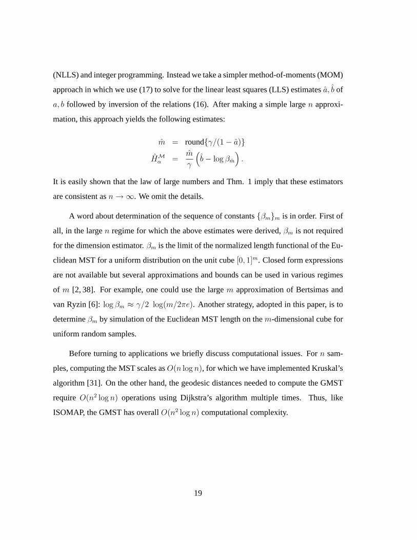
Figure 1: The S-shaped surface manifold and corresponding GMST (k = 7) graph on 400sample points.

5 Applications

We illustrate the performance of the GMST algorithm on manifolds of known dimension

as well as on a real data set consisting of face images. In all the simulations we fixed

the parametersγ = 1 and p1 = n − Q, . . . , pQ = n − 1. With regards to intrinsic

dimension estimation, we compare our algorithm to ISOMAP. In ISOMAP, similarly to

PCA, intrinsic dimension is usually estimated by detecting changes in the residual fitting

errors as a function of subspace dimension.

5.1 S-Shaped Surface

The first manifold considered is the standard2-dimensional S-shaped surface [34] em-

bedded inR3 (Fig. 1). Fig. 2 shows the evolution of the average GMST lengthLn as a

function of the number of samples, for a random set of i.i.d. points uniformly distributed

on the surface.

To compare the dimension estimation performance of the GMST method to ISOMAP

we ran a Monte Carlo simulation. For each of several sample sizes,30 independent sets

of i.i.d. random vectors uniformly distributed on the surface were generated. We then

counted the number of times that the intrinsic dimension was correctly estimated. To au-

20

200 250 300 350 400 450 500 550

32

34

36

38

40

42

44

46

48

50

n

GM

ST

leng

th

(a)

5.3 5.4 5.5 5.6 5.7 5.8 5.9 6 6.1 6.2 6.33.45

3.5

3.55

3.6

3.65

3.7

3.75

3.8

3.85

3.9

log nlo

g G

MS

T le

ngth

(b)

6.382 6.384 6.386 6.388 6.39 6.392 6.394

3.913

3.914

3.915

3.916

3.917

3.918

3.919

3.92

log n

log

GM

ST

leng

th

Ln

LS fit of Ln

(c)

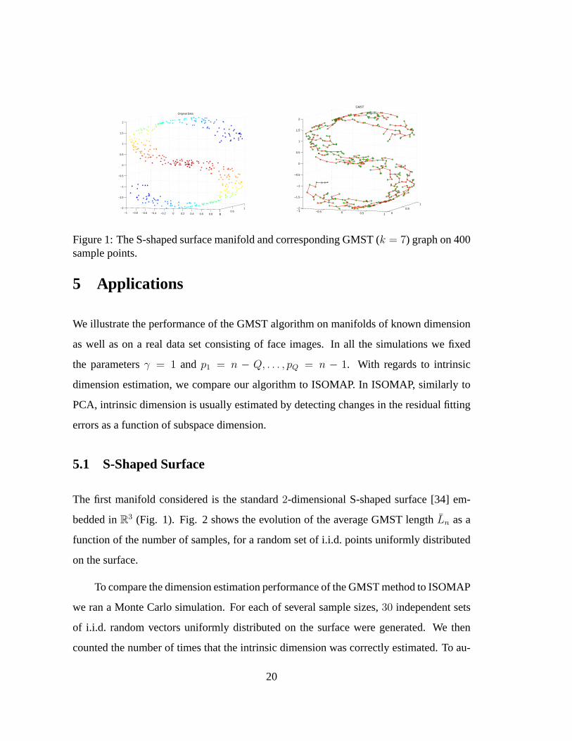
Figure 2: (a) plot of the average GMST lengthLn for the S-shaped manifold as a functionof the number of samples; (b) log-log plot of (a); (c) blowup of the last ten points in (b)and its linear least squares fit. The estimated slope isa = 0.4976 which impliesm = 2.(k = 7, N = 5)

tomatically estimate dimension with ISOMAP, we follow a standard PCA order estima-

tion procedure. Specifically, we graph the residual variance of the MDS fit as a function

of the PCA dimension and try to detect the “elbow” at which residuals cease to decrease

“significantly” as estimated dimension increases [36]. The elbow detector is implemented

by a simple minimum angle threshold rule. Table 3 shows the results of this experiment.

As it can be observed, the GMST algorithm outperforms ISOMAP in terms of dimension

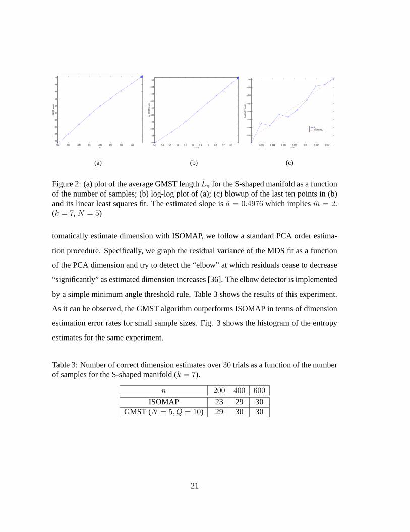
estimation error rates for small sample sizes. Fig. 3 shows the histogram of the entropy

estimates for the same experiment.

Table 3: Number of correct dimension estimates over30 trials as a function of the numberof samples for the S-shaped manifold (k = 7).

n 200 400 600

ISOMAP 23 29 30GMST (N = 5, Q = 10) 29 30 30

21

2 2.5 3 3.5 4 4.5 50

1

2

3

4

5

6

True estimated entropy (bits)

His

togr

am

Sample Mean

Figure 3: Histogram of entropy estimates over 30 trials of 600 samples uniformly dis-tributed on the S-shaped manifold (k = 7, N = 5, Q = 10). True entropy (”true”) wascomputed analytically from the area of S curve supporting the uniform distribution ofmanifold samples.

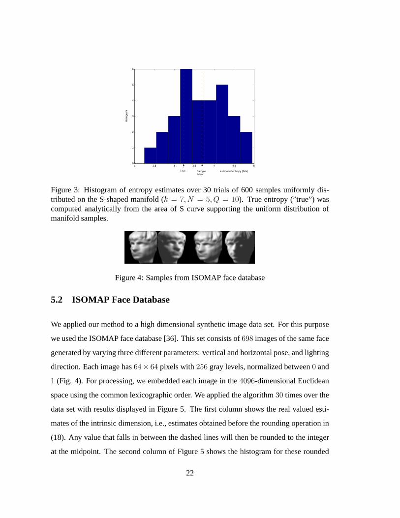
Figure 4: Samples from ISOMAP face database

5.2 ISOMAP Face Database

We applied our method to a high dimensional synthetic image data set. For this purpose

we used the ISOMAP face database [36]. This set consists of698 images of the same face

generated by varying three different parameters: vertical and horizontal pose, and lighting

direction. Each image has64× 64 pixels with256 gray levels, normalized between0 and

1 (Fig. 4). For processing, we embedded each image in the4096-dimensional Euclidean

space using the common lexicographic order. We applied the algorithm30 times over the

data set with results displayed in Figure 5. The first column shows the real valued esti-

mates of the intrinsic dimension, i.e., estimates obtained before the rounding operation in

(18). Any value that falls in between the dashed lines will then be rounded to the integer

at the midpoint. The second column of Figure 5 shows the histogram for these rounded

22

2 3 4 5 60

5

10

15

20

25

30

dimension estimate0 10 20 30

2

2.5

3

3.5

4

4.5

5

5.5

simulation number

real

val

ued

dim

ensi

on e

stim

ate

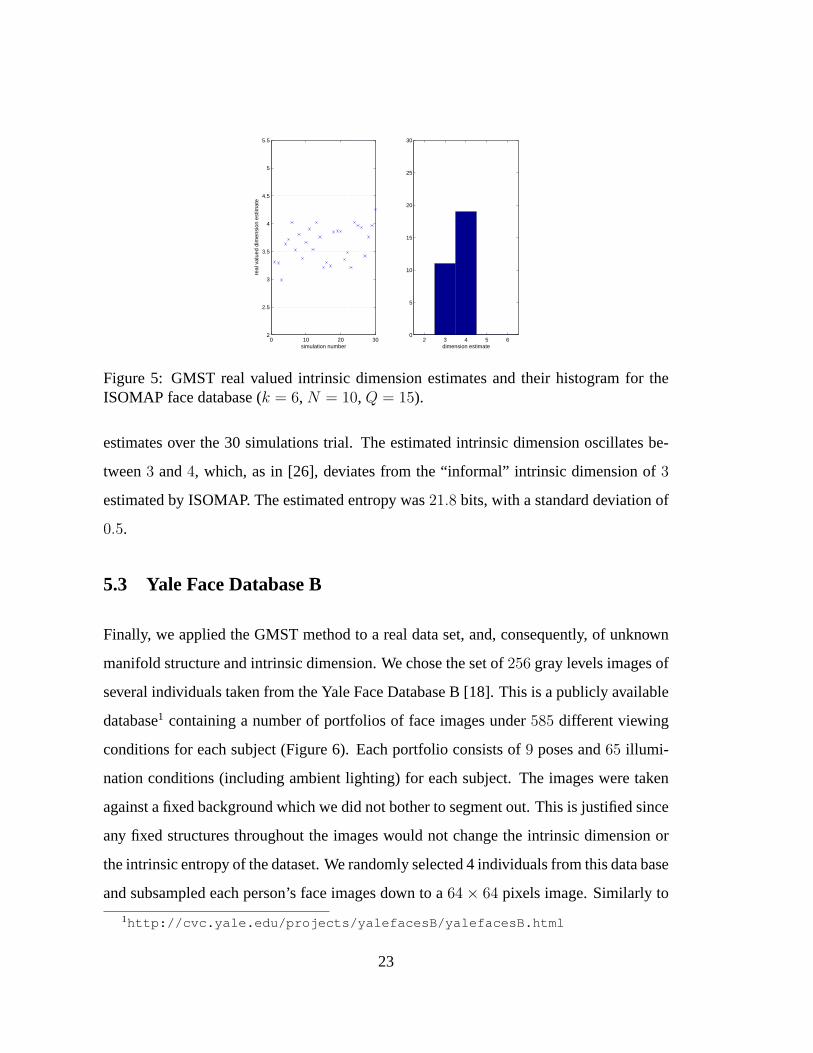
Figure 5: GMST real valued intrinsic dimension estimates and their histogram for theISOMAP face database (k = 6, N = 10, Q = 15).

estimates over the 30 simulations trial. The estimated intrinsic dimension oscillates be-

tween3 and4, which, as in [26], deviates from the “informal” intrinsic dimension of3

estimated by ISOMAP. The estimated entropy was21.8 bits, with a standard deviation of

0.5.

5.3 Yale Face Database B

Finally, we applied the GMST method to a real data set, and, consequently, of unknown

manifold structure and intrinsic dimension. We chose the set of256 gray levels images of

several individuals taken from the Yale Face Database B [18]. This is a publicly available

database1 containing a number of portfolios of face images under585 different viewing

conditions for each subject (Figure 6). Each portfolio consists of9 poses and65 illumi-

nation conditions (including ambient lighting) for each subject. The images were taken

against a fixed background which we did not bother to segment out. This is justified since

any fixed structures throughout the images would not change the intrinsic dimension or

the intrinsic entropy of the dataset. We randomly selected 4 individuals from this data base

and subsampled each person’s face images down to a64 × 64 pixels image. Similarly to

1http://cvc.yale.edu/projects/yalefacesB/yalefacesB.html

23

Face 1

Face 2

Face 3

Face 4

Figure 6: Samples from Yale face database B

3 4 5 6 70

5

10

15

20

25

30

dimension estimate0 10 20 30

3.5

4

4.5

5

5.5

6

6.5

7

7.5

simulation number

real

val

ued

dim

ensi

on e

stim

ate

Figure 7: GMST real valued intrinsic dimension estimates and histogram for face 2 in theYale face database B (k = 7, N = 10, Q = 20).

the ISOMAP face data set, we normalized the pixel values between0 and1. Figure 7

displays the results of running30 simulations of the algorithm using face2. The intrinsic

dimension estimate is between5 and6. Figure 8 shows the corresponding residual vari-

ance plots used by ISOMAP to estimate intrinsic dimension. From these plots it is not

obvious how to determine the “elbow” at which the residuals cease to decrease “signifi-

cantly” with added dimensions. This illustrates one of the major drawbacks of ISOMAP

(and other spectral based methods like PCA) as an intrinsic dimension estimator, as it

relies on a specific eigenstructure that may not exist in real data. The simple minimum

24

1 2 3 4 5 6 7 8 9 100.05

0.1

0.15

0.2

0.25

0.3

0.35

0.4

0.45

ISOMAP dimensionality

Res

idua

l var

ianc

e

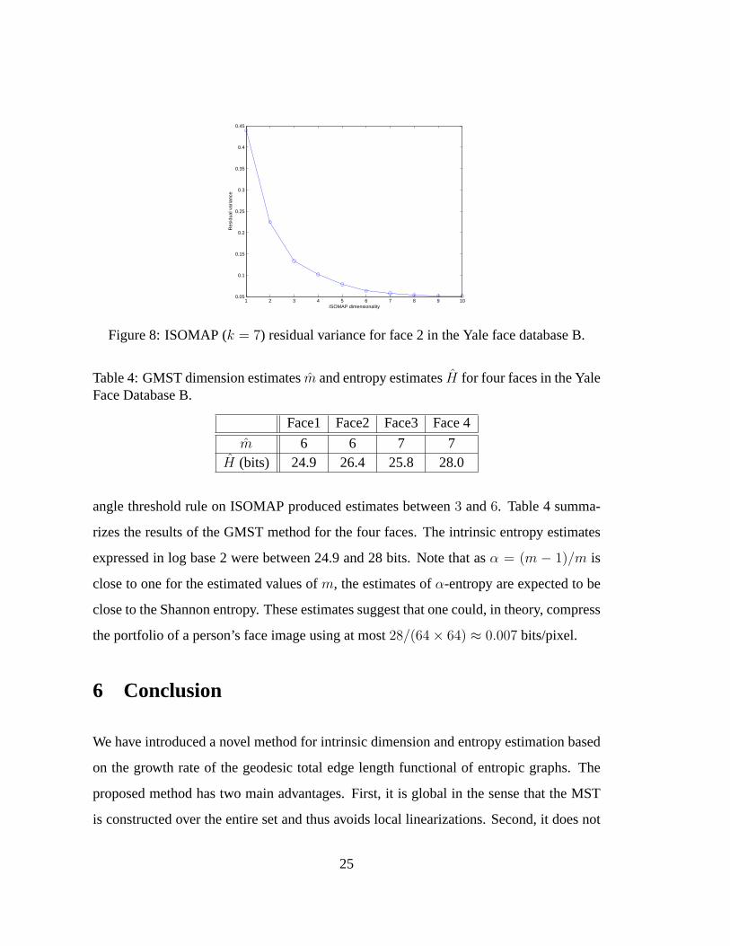
Figure 8: ISOMAP (k = 7) residual variance for face 2 in the Yale face database B.

Table 4: GMST dimension estimatesm and entropy estimatesH for four faces in the YaleFace Database B.

Face1 Face2 Face3 Face 4

m 6 6 7 7H (bits) 24.9 26.4 25.8 28.0

angle threshold rule on ISOMAP produced estimates between3 and6. Table 4 summa-

rizes the results of the GMST method for the four faces. The intrinsic entropy estimates

expressed in log base 2 were between 24.9 and 28 bits. Note that asα = (m − 1)/m is

close to one for the estimated values ofm, the estimates ofα-entropy are expected to be

close to the Shannon entropy. These estimates suggest that one could, in theory, compress

the portfolio of a person’s face image using at most28/(64× 64) ≈ 0.007 bits/pixel.

6 Conclusion

We have introduced a novel method for intrinsic dimension and entropy estimation based

on the growth rate of the geodesic total edge length functional of entropic graphs. The

proposed method has two main advantages. First, it is global in the sense that the MST

is constructed over the entire set and thus avoids local linearizations. Second, it does not

25

require reconstructing the manifold or estimating the multivariate density of the samples.

We validated the new method by testing it on synthetic manifolds of known dimension

and on high dimensional real data sets.

We are currently working on extending Thm. 1 and Corollary 1 to general Riemann

manifolds, thus avoiding any assumptions about global embeddings and eliminating the

effect of the Jacobian on the intrinsic entropy. We are also studying the use of entropic

graphs that bypass the complex step of geodesic estimation. In [11], we considerk-nearest

neighbor graphs due to their low complexity an local properties. The simple bootstrap

resampling step that we have used in the GMST estimator causes a small negative bias

in the dimension estimate for flat linear manifolds. Future work includes development

of GMST resampling bias correction, characterization of the statistics in the linear model

(15) and the study of the effect of additive noise on the manifold samples.

Acknowledgments

The authors acknowledge and thank the creators of Yale Face Database B for mak-

ing their face image data publicly available. The authors would also like to thank Huzefa

Neemuchwala and Arpit Almal for their help in acquiring and processing these face im-

ages. This work was partially supported by the DARPA MURI program under ARO con-

tract DAAD19-02-1-0262 and by the NIH Cancer Institute under grant 1PO1 CA87634-

01.

26

References

[1] K. S. Alexander, “The RSW theorem for continuum percolation and the CLT for Eu-

clidean minimal spanning trees,”Ann. Applied Probab., vol. 6, pp. 466–494, 1996.

[2] F. Avram and D. Bertsimas, “The minimum spanning tree constant in geometrical

probability and under the independent model: a unified approach,”Ann. Applied

Probab., vol. 9, pp. 223–231, 1990.

[3] J. Beardwood, J. H. Halton, and J. M. Hammersley, “The shortest path through many

points,”Proc. Cambridge Philosophical Society, vol. 55, pp. 299–327, 1959.

[4] M. Belkin and P. Niyogi, “Laplacian eigenmaps and spectral techniques for embed-

ding and clustering,” inAdvances in Neural Information Processing Systems, Volume

14, T. G. Diettrich, S. Becker, and Z. Ghahramani, editors, MIT Press, 2002.

[5] M. Bernstein, V. de Silva, J. C. Langford, and J. B. Tenenbaum, “Graph approx-

imations to geodesics on embedded manifolds,” Technical report, Department of

Psychology, Stanford University, 2000.

[6] D. Bertsimas and G. van Ryzin, “An aysmptotic determination of the minimum

spanning tree and minimum matching constants in geometrical probability,”Oper.

Research Letters, vol. 2, pp. 113–130, 1992.

[7] W. Boothby,An introduction to differentiable manifolds and Riemannian geometry,

Academic, San Diego, Calif., rev. 2nd edition, 2003.

[8] F. Camastra and A. Vinciarelli, “Estimating the intrinsic dimension of data with a

fractal-based method,”IEEE Trans. on Pattern Analysis and Machine Intelligence,

vol. PAMI-24, no. 10, pp. 1404–1407, October 2002.

[9] M. Carmo,Differential geometry of curves and surfaces, Prentice-Hall, Englewood

Cliffs, N.J., 1976.

27

[10] M. Carmo,Riemannian geometry, Birkhauser, Boston, 1992.

[11] J. A. Costa and A. O. Hero, “Entropic graphs for manifold learning,” inProc.

of IEEE Asilomar Conf. on Signals, Systems, and Computers, Pacific Grove, CA,

November 2003.

[12] T. Cover and J. Thomas,Elements of Information Theory, Wiley, New York, 1991.

[13] T. Cox and M. Cox,Multidimensional Scaling, Chapman & Hall, London, 1994.

[14] I. Csiszar, “Generalized cutoff rates and Renyi’s information measures,”IEEE

Trans. on Inform. Theory, vol. IT-41, no. 1, pp. 26–34, January 1995.

[15] V. de Silva and J. B. Tenenbaum, “Global versus local methods in nonlinear dimen-

sionality reduction,” inNeural Information Processing Systems 15 (NIPS), Vancou-

ver, Canada, Dec. 2002.

[16] V. de Silva and J. B. Tenenbaum, “Unsupervised learning of curved manifolds,” in

Nonlinear estimation and classification, D. Denison, M. H. Hansen, C. C. Holmes,

B. Mallick, and B. Yu, editors, Springer-Verlag, New York, 2002.

[17] D. Donoho and C. Grimes, “Hessian eigenmaps: locally linear embedding tech-

niques for high dimensional data,”Proc. Nat. Acad. of Sci., vol. 100, no. 10, pp.

5591–5596, 2003.

[18] A. Georghiades, P. Belhumeur, and D. Kriegman, “From few to many: Illumination

cone models for face recognition under variable lighting and pose,”IEEE Trans. on

Pattern Analysis and Machine Intelligence, vol. PAMI-23, no. 6, pp. 643–660, 2001.

[19] A. Gersho, “Asymptotically optimal block quantization,”IEEE Trans. on Inform.

Theory, vol. IT-28, pp. 373–380, 1979.

28

[20] A. Hero, J. Costa, and B. Ma, “Convergence rates of minimal graphs with random

vertices,” submitted toIEEE Trans. on Inform. Theory, 2002,www.eecs.umich.

edu/˜hero/det_est.html .

[21] A. Hero and O. Michel, “Asymptotic theory of greedy approximations to minimal

k-point random graphs,”IEEE Trans. on Inform. Theory, vol. IT-45, no. 6, pp. 921–

1939, September 1999.

[22] A. Hero, B. Ma, O. Michel, and J. Gorman, “Applications of entropic spanning

graphs,”IEEE Signal Processing Magazine, vol. SPM-19, no. 5, pp. 85–95, October

2002.

[23] A. Hero and O. Michel, “Estimation of Renyi information divergence via pruned

minimal spanning trees,” inIEEE Workshop on Higher Order Statistics, Caesaria,

Israel, Jun. 1999.

[24] X. Huo and J. Chen, “Local linear projection (LLP),” inProc. of First Workshop on

Genomic Signal Processing and Statistics (GENSIPS), 2002.

[25] A. K. Jain and R. C. Dubes,Algorithms for clustering data, Prentice Hall, Engle-

wood Cliffs, NJ, 1988.

[26] B. Kegl, “Intrinsic dimension estimation using packing numbers,” inNeural Infor-

mation Processing Systems: NIPS, Vancouver, CA, Dec. 2002.

[27] M. Kirby, Geometric Data Analysis: An Empirical Approach to Dimensionality Re-

duction and the Study of Patterns, Wiley-Interscience, 2001.

[28] V. I. Koltchinskii, “Empirical geometry of multivariate data: A deconvolution ap-

proach,”Annals of Statistics, vol. 28, no. 2, pp. 591–629, 2000.

29

[29] F. Memoli and G. Sapiro, “Fast computation of weighted distance functions and

geodesics on implicit hyper-surfaces,”Journal of Computationals Physics, vol. 73,

pp. 730–764, 2001.

[30] F. Memolia, G. Sapiro, and S. Osher, “Solving variational problems and partial dif-

ferentyial equations mapping into general target manifolds,” Technical Report 1827,

IMA, January 2003.

[31] H. Neemuchwala, A. O. Hero, and P. Carson, “Image registration using entropy

measures and entropic graphs,”to appear in European Journal of Signal Processing,

Special Issue on Content-based Visual Information Retrieval, 2003.

[32] D. N. Neuhoff, “On the asymptotic distribution of the errors in vector quantization,”

IEEE Trans. on Inform. Theory, vol. IT-42, pp. 461–468, March 1996.

[33] K. Pettis, T. Bailey, A. Jain, and R. Dubes, “An intrinsic dimensionality estimator

from near-neighbor information,”IEEE Trans. on Pattern Analysis and Machine

Intelligence, vol. PAMI-1, no. 1, pp. 25–36, 1979.

[34] S. Roweis and L. Saul, “Nonlinear dimensionality reduction by locally linear imbed-

ding,” Science, vol. 290, no. 1, pp. 2323–2326, 2000.

[35] J. M. Steele,Probability theory and combinatorial optimization, volume 69 of

CBMF-NSF Regional Conferences in Applied Mathematics, Society for Industrial

and Applied Mathematics (SIAM), 1997.

[36] J. B. Tenenbaum, V. de Silva, and J. C. Langford, “A global geometric framework

for nonlinear dimensionality reduction,”Science, vol. 290, pp. 2319–2323, 2000.

[37] P. Verveer and R. Duin, “An evaluation of intrinsic dimensionality estimators,”IEEE

Trans. on Pattern Analysis and Machine Intelligence, vol. PAMI-17, no. 1, pp. 81–

86, January 1995.

30

[38] J. E. Yukich,Probability theory of classical Euclidean optimization problems, vol-

ume 1675 ofLecture Notes in Mathematics, Springer-Verlag, Berlin, 1998.

31