Geodesic convexity & covariance estimation - IRIT · based power control for general SIR regime. In...

G-convexity Covariance Non Gaussian Kronecker Symmetry

Geodesic convexity & covariance estimation

Ami Wiesel

School of Engineering and Computer ScienceHebrew University of Jerusalem, Israel

June 28, 2013

1 / 40


Acknowledgments

Teng Zhang (Princeton).

Maria Greco (Universita di Pisa).

Ilya Soloveychik (Hebrew University).

Alba Sloin (Hebrew University).

2 / 40


1 Geodesic convexity

2 Covariance estimation

3 Non Gaussian

4 Kronecker models

5 Symmetry constraints

3 / 40


Outline



3 Non Gaussian

4 Kronecker models


4 / 40


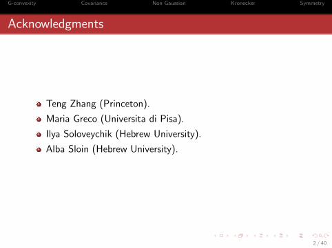
Convexity

Convex function

f (xt) ≤ tf (x1) + (1− t) f (x0)

xt = tx1 + (1− t)x0

f x0( )

f xt( )

f x1( )

Local solutions are easy to find and globally optimal!

Easy to generalize:

Building bricks: linear, quadratic, norms...Rules: convex+convex=convex,...

5 / 40


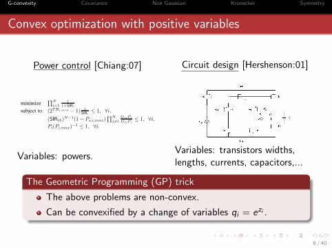
Convex optimization with positive variables

Power control [Chiang:07] Circuit design [Hershenson:01]

2646 IEEE TRANSACTIONS ON WIRELESS COMMUNICATIONS, VOL. 6, NO. 7, JULY 2007

B. Examples of successive convex approximation

1) Logarithmic approximation for GP: In [17], [18], anonconvex problem involving the function log(1 + SIR) isapproximated by a + b log(SIR) for some a and b that satisfythe above three conditions.

2) Single condensation method for GP: ComplementaryGPs involve upper bounds on the ratio of posynomials as in(9); they can be turned into GPs by approximating the denomi-nator of the ratio of posynomials, g(x), with a monomial g̃(x),but leaving the numerator f(x) as a posynomial.

Lemma 1: Let g(x) =!

i ui(x) be a posynomial. Then

g(x) ! g̃(x) ="

i

#ui(x)

!i

$!i

. (11)

If, in addition, !i = ui(x0)/g(x0), "i, for any fixed positivex0, then g̃(x0) = g(x0), and g̃(x0) is the best local monomialapproximation to g(x0) near x0 in the sense of first orderTaylor approximation.

Proof: The arithmetic-geometric mean inequality statesthat

!i !ivi ! %

i v!i

i , where v # 0 and ! $ 0, 1T ! =1. Letting ui = !ivi, we can write this basic inequality as!

i ui ! %i (ui/!i)!i . The inequality becomes an equality if

we let !i = ui/!

i ui, "i, which satisfies the condition that! $ 0 and 1T ! = 1. The best local monomial approximationg̃(x0) of g(x0) near x0 can be easily verified [4].

Proposition 3: The approximation of a ratio of posynomialsf(x)/g(x) with f(x)/g̃(x), where g̃(x) is the monomialapproximation of g(x) using the arithmetic-geometric meanapproximation of Lemma 1, satisfies the three conditions forthe convergence of the successive approximation method.

Proof: Conditions (1) and (2) are clearly satisfied sinceg(x) ! g̃(x) and g̃(x0) = g(x0) (Lemma 1). Condition (3) iseasily verified by taking derivatives of g(x) and g̃(x).

Suppose we want to minimize f0(x) subject to an equalityconstraint on a ratio of posynomials f(x)/g(x) = 1. Then,we can rewrite this as minimizing f0(x) + "t subject tof(x)/g(x) % 1 and f(x)/g(x) ! 1 & t where " is a suf-ficiently large number to guarantee that the optimum solutionwill have t ' 0.5 The second constraint can be rewritten asg(x)/(f(x) + tg(x)) % 1 where we can apply the singlecondensation method to the denominators of both constraints.

3) Double condensation method for GP[1]: Another choiceof approximation is to make a double monomial approxi-mation for both the denominator and numerator in (9). Wecan still use the arithmetic-geometric mean approximation ofLemma 1 as a monomial approximation for the denominator.But, Lemma 1 cannot be used as a monomial approximationfor the numerator. To satisfy the three conditions for theconvergence of the successive approximation method, a mono-mial approximation for the numerator f(x) should satisfyf(x) % f̃(x).

C. Applications to power control

Figure 5 shows a block diagram of the approach of GP-based power control for general SIR regime. In the high SIRregime, we need to solve only one GP. In the medium to low

5In our numerical analysis, we use ! = 1 + k at the k-th iteration.

(High SIR) OriginalProblem

Solve1 GP

(Mediumto

Low SIR)

OriginalProblem

SPComplementaryGP (Condensed)

Solve1 GP

!

! ! !

"

Fig. 5. GP-based power control for general SIR regime.

SIR regimes, we solve truly nonconvex power control prob-lems that cannot be turned into convex formulation through aseries of GPs.

GP-based power control problems in the medium to low SIRregimes become SP (or, equivalently, Complementary GP),which can be solved by the single or double condensationmethod. We focus on the single condensation method here.Consider a representative problem formulation of maximizingtotal system throughput in a cellular wireless network subjectto user rate and outage probability constraints in problem (6),which can be explicitly written out as

minimize%N

i=11

1+SIRi

subject to (2TRi,min & 1) 1SIRi

% 1, "i,

(SIRth)N!1(1 & Po,i,max)%N

j "=iGijPj

GiiPi% 1, "i,

Pi(Pi,max)!1 % 1, "i.(12)

All the constraints are posynomials. However, the objectiveis not a posynomial, but a ratio between two posynomialsas in (9). This power control problem can be solved by thecondensation method by solving a series of GPs. Specifically,we have the following single-condensation algorithm:

Algorithm Single condensation GP power controlInput An initial feasible power vector P.Output A power allocation that satisfies the KKT condi-

tions.1) Evaluate the denominator posynomial of the objective

function in (12) with the given P.2) Compute for each term i in this posynomial,

!i =value of ith term in posynomial

value of posynomial.

3) Condense the denominator posynomial of the (12) ob-jective function into a monomial using (11) with weights !i.

4) Solve the resulting GP using an interior point method.5) Go to step 1 using P of step 4.6) Terminate the kth loop if ( P(k) & P(k!1) (% # where

# is the error tolerance for exit condition.As condensing the objective in the above problem gives

us an underestimate of the objective value, each GP in thecondensation iteration loop tries to improve the accuracy of theapproximation to a particular minimum in the original feasibleregion. All three conditions for convergence in subsection IV.Aare satisfied, and the algorithm is provably convergent. Em-pirically through extensive numerical experiments, we observethat it often compute the globally optimal power allocation.

Example 4. We consider a wireless cellular network with 3users. Let T = 10!6s, Gii = 1.5, and generate Gij , i )= j, as

2 IEEE TRANSACTIONS ON COMPUTER-AIDED DESIGN OF INTEGRATED CIRCUITS AND SYSTEMS, VOL. 20, NO. 1, JANUARY 2001

Fig. 1. Two-stage op-amp considered herein.

ysis, …) are due to the formulation of the design problem as aconvex optimization problem. Geometric programming (whenreformulated as described in Section II-A) is just a special typeof convex optimization problem.Although general convex prob-lems can be solved efficiently, the special structure of geometricprogramming can be exploited to obtain an even more efficientsolution algorithm.The method we present can be applied to a wide variety of

amplifier architectures, but in this paper, we apply the methodto a specific two-stage CMOS op-amp. The authors show howthe method extends to other architectures in [49] and [50]. Alonger version of this paper, which includes more detail aboutthe models, some of the derivations, and SPICE simulationparameters, is available at the authors’ web site [51]. Relatedwork has been reported in several conference publications, e.g.,[48]–[50].

A. The Two-Stage AmplifierThe specific two-stage CMOS op-amp we consider is shown

in Fig. 1. The circuit consists of an input differential stage withactive load followed by a common-source stage also with ac-tive load. An output buffer is not used; this amplifier is as-sumed to be part of a very large scale integration (VLSI) systemand is only required to drive a fixed on-chip capacitive load ofa few picofarads. This op-amp architecture has many advan-tages: high open-loop voltage gain, rail-to-rail output swing,large common-mode input range, only one frequency compen-sation capacitor, and a small number of transistors. Its maindrawback is the nondominant pole formed by the load capac-itance and the output impedance of the second stage, whichreduces the achievable bandwidth. Another potential disadvan-tage is the right half-plane zero that arises from the feedforwardsignal path through the compensating capacitor. Fortunately, thezero is easily removed by a suitable choice for the compensationresistor (see [2]).This op-amp is a widely used general purpose op-amp [88];

it finds applications, for example, in switched capacitor filters[23], analog-to-digital converters [60], [72], and sensing circuits[85].There are 18 design parameters for the two-stage op-amp:• Thewidths and lengths of all transistors, i.e.,and .

• The bias current .• The value of the compensation capacitor .

The compensation resistor is chosen in a specific way that isdependent on the design parameters listed above (and describedin Section V). There are also a number of parameters that weconsider fixed, e.g., the supply voltages and , the ca-pacitive load , and the various process and technology pa-rameters associated with the MOS models. To simplify some ofthe equations we assume (without any loss of generality) that

.

B. Other ApproachesThere is a huge literature, which goes back more than 20

years, on computer-aided design (CAD) of analog circuits. Agood survey of early research can be found in the survey [11];more recent papers on analog-circuit CAD tools include [4],[12], [13]. The problem we consider in this paper, i.e., selectionof component values and transistor dimensions, is only a part ofa complete analog-circuit CAD tool. Other parts, which we donot consider here, include topology selection (see [66]) and ac-tual circuit layout (see, e.g., ILAC [27], KOAN/ANAGRAM II[15]). The part of the CADprocess that we consider lies betweenthese two tasks; the remainder of the discussion is restricted tomethods dealing with component and transistor sizing.1) Classical Optimization Methods: General-purpose clas-

sical optimization methods, such as steepest descent, sequen-tial quadratic programming, and Lagrange multiplier methods,have been widely used in analog-circuit CAD. These methodscan be traced back to the survey paper [11]. The widely usedgeneral-purpose optimization codes NPSOL [39] and MINOS[71] are used in [25], [64], and [67]. LANCELOT [16], an-other general-purpose optimizer, is used in [22]. Other CADapproaches based on classical optimization methods, and exten-sions such as a minimax formulation, include the one describedin [47], [61], and [63], OAC [78], OPASYN [56], CADICS [54],WATOPT [31], and STAIC [45]. The classical methods can beused with more complicated circuit models, including even fullSPICE simulations in each iteration, as in DELIGHT.SPICE[75] (which uses the general-purpose optimizer DELIGHT [76])and ECSTASY [86].The main advantage of these methods is the wide variety of

problems they can handle; the only requirement is that the per-formance measures, along with one or more derivatives, can becomputed. The main disadvantage of the classical optimizationmethods is they only find locally optimal designs. This meansthat the design is at least as good as neighboring designs, i.e.,small variations of any of the design parameters results in aworse (or infeasible) design. Unfortunately this does not meanthe design is the best that can be achieved, i.e., globally optimal;it is possible (and often happens) that some other set of designparameters, far away from the one found, is better. The sameproblem arises in determining feasibility: a classical (local) op-timization method can fail to find a feasible design, even thoughone exists. Roughly speaking, classical methods can get stuck atlocal minima. This shortcoming is so well known that it is oftennot even mentioned in papers; it is taken as understood.The problem of nonglobal solutions from classical optimiza-

tion methods can be treated in several ways. The usual approach

Variables: powers.Variables: transistors widths,lengths, currents, capacitors,...

The Geometric Programming (GP) trick

The above problems are non-convex.

Can be convexified by a change of variables qi = ezi .

6 / 40


Convexity with positive variables

Exp: ezi are convex in zi .

Log-sum-exp: log∑

i ezi is convex in zi .

If f (ez) is convex in z then f (ez1+z2) is convex in z1, z2.

ez transforms sums into products!

The Geometric Programming (GP) trick

Minimize products of positive numbers qi ≥ 0 using ezi .

7 / 40


Convexity with positive definite matrices Qi � 0

Today: GP with positive definite matrices

Can we minimize powers aTQ±1a?

Can we minimize log determinants log|Q|?Can we minimize products Q1 ⊗Q2?

The answers are YES!

But the solution is not a simple change of variables.

Instead, we turn to geodesic convexity.

8 / 40


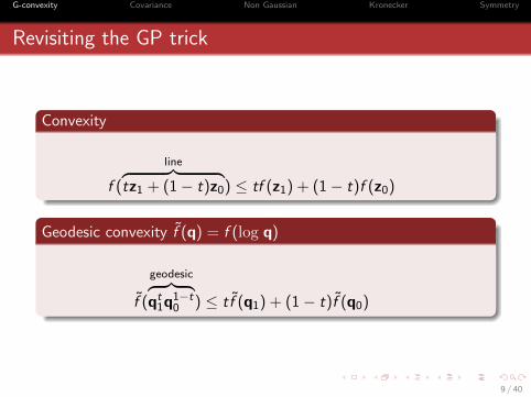
Revisiting the GP trick

Convexity

f (

line︷︸︸︷tz1 + (1− t)z0) ≤ tf (z1) + (1− t)f (z0)

Geodesic convexity f̃ (q) = f (log q)

f̃ (

geodesic︷︸︸︷qt1q

1−t0 ) ≤ tf̃ (q1) + (1− t)f̃ (q0)

9 / 40


Geodesic convexity [Rapcsak 91], [Liberti 04]

For any q1,q0 ∈ D we define a geodesicqt ∈ D parameterized by t ∈ [0, 1].

€

q0

€

q1

€

qt

A function f (q) is g-convex in q ∈ D if

f (qt) ≤ tf (q1) + (1− t) f (q0) ∀ t ∈ [0, 1].

Properties

Any local minimizer of f (q) over D is a global minimizer.

g-convex + g-convex = g-convex.

10 / 40


From scalars to matrices

We do not know the matrix version of ex .

We do know how to generalize the geodesics qt = qt1q1−t0 .

Geodesic between Q0 � 0 and Q1 � 0

Qt = Q120

(Q− 1

20 Q1Q

− 12

0

)t

Q120 , t ∈ [0, 1].

11 / 40


Powers (matrix case)

Theorem

The function

f (Q) = aTQ±1a

is g-convex in Q � 0.

Proof: eigenvalue decomposition reduces to scalar case.

12 / 40


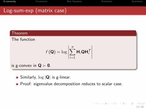
Log-sum-exp (matrix case)

Theorem

The function

f (Q) = log

∣∣∣∣∣n∑

i=1

HiQHTi

∣∣∣∣∣

is g-convex in Q � 0.

Similarly, log |Q| is g-linear.

Proof: eigenvalue decomposition reduces to scalar case.

13 / 40


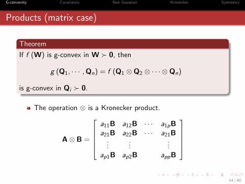
Products (matrix case)

Theorem

If f (W) is g-convex in W � 0, then

g (Q1, · · · ,Qn) = f (Q1 ⊗Q2 ⊗ · · · ⊗Qn)

is g-convex in Qi � 0.

The operation ⊗ is a Kronecker product.

A⊗ B =

a11B a12B · · · a1pBa21B a22B · · · a21B

......

...ap1B ap2B appB

14 / 40


Invariance to orthogonal operators

A set S is g-convex if

Q0,Q1 ∈ S ⇒ Qt ∈ S.

Local minimas over g-convex sets are global.

Theorem

For orthonormal U, the set {Q : Q = UQUT} is g-convex.

Proof: Matrix commutativity properties QU = UQ.

Trivial in scalar case.

15 / 40


Summary

aTQ±1a is g-convex.

log∣∣∑n

i=1HiQHTi

∣∣ is g-convex.

Qi ⊗ · · · ⊗Qj preserves g-convexity.

{Q : Q = UQUT} is g-convex.

16 / 40


Outline



3 Non Gaussian

4 Kronecker models


17 / 40


Covariance estimation

x: p-dimensional random vector.

Mean E{x} = 0, covariance Σ = E[xxT

].

{xi}ni=1: n independent & identically distributed realizations.

Goal

Problem: Derive Σ̂ ({xi}ni=1) to estimate Σ.

Solution: Maximum likelihood.

Emphasis on the hard non-Gaussian and structured cases.

18 / 40


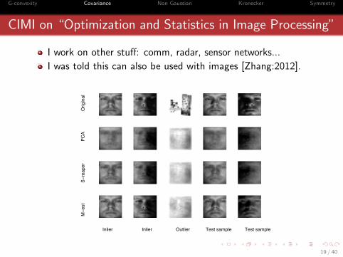
CIMI on “Optimization and Statistics in Image Processing”

I work on other stuff: comm, radar, sensor networks...

I was told this can also be used with images [Zhang:2012].7

Inlier Inlier Outlier Test sample Test sample

M−e

st

S−r

eape

r

PCA

O

rigin

al

Fig. 4. The projection of images to the fitted subspace.

300 400 500 600 700 800 900 1000100

200

300

400

500

600

700

800

900

1000

Distance to the PCA subspace

Dis

tanc

e to

the

robu

st s

ubsp

ace

M−estimatorS−reaper

Fig. 5. Ordered distances of the 32 test images to the fitted 9-dimensionalsubspaces by Algorithm 1, S-reaper and PCA.

for the test images. This observation can also be quantitativelyverified by checking the distances of 32 test images to the fittedsubspace by PCA, S-reaper and out algorithm, which is shownin Figure IV-E. The subspace generated by our algorithm hassmaller distances to the test images, which explain the betterperformance of our algorithm in Figure IV-E.Besides, in this experiment our algorithm performs much

faster than S-Reaper; our algorithm costs 4.4 seconds ona machine with Intel Core 2 Duo CPU at 3.00GHz and6GB memory, while S-reaper cost 40 seconds. it is expectedsince there is an additional eigenvalue decomposition in eachiteration of the S-Reaper algorithm.

V. DISCUSSION

In this paper we have investigated an M-estimator forcovariance estimation, and proved that this estimator canfind the underlying subspace exactly under a rather weak

assumption. We also demonstrated the virtue of this methodsby experiments on simulated data sets and real data sets.An open question is that, if we can have a theoretical

guarantee on the robustness of our algorithm to noise andtherefore verify the empirical performance in Section IV-D.We find it difficult to apply the commonly used perturbationanalysis in [35, Section 2.7] or [34, Theorem 2], which arebased on the size of the perturbation of the objective function,since the objective function F (!) at a singular matrix isundefined.An interesting direction is to extend the idea of geodesi-

cal convexity to other problems. Euclidean metric betweenmatrices is usually used and under this metric the set of allpositive definite matrices is considered as a cone. Howeverin this work we consider the set of all positive matrices as amanifold and use the Riemmannian metric between matrices.It turns out that while F (!) in nonconvex in Euclidean metric,it is convex in Riemmannian metric, and this formulation ismore powerful than similar formulations that are convex inEuclidean metric [35], [17]. It would be interesting if there areother optimization problems with the property of geodesicalconvexity.

VI. ACKNOWLEDGEMENTThe author would like to thank Michael Mccoy for reading

an earlier version of this manuscript and for helpful comments.The author is grateful to Lek Heng Lim for introducing thebook [4] and helpful discussions.

VII. APPENDIXA. Proof of Lemma III.2

Proof: Geodesical convexity of F (!) follows from (III.2)and Lemma II.1. Therefore we only need to prove (III.2) forgeodesic convexity.We will prove (III.2) by showing that, if !3 ! S++(D) is

the geometric mean of !1,!2 ! S++(D), then we have

ln(det(!1)) + ln(det(!2)) = 2 ln(det(!3)), (VII.1)

and

ln(xT !1x) + ln(xT !2x) " 2 ln(xT !3x). (VII.2)

We start with the proof of (VII.1). Use (II.2) with t = 12 ,

we have

!3!!11 !3

=!121 (!

! 12

1 !3!! 1

21 )

12 !

121 !!1

1 !121 (!

! 12

1 !3!! 1

21 )

12 !

121

=!2. (VII.3)

Using (VII.3), (VII.1) can be proved as follows:

det(!2) = det(!3!!11 !3) = det(!3) det(!!1

1 ) det(!3)

=det(!3)2/ det(!1).

To prove (VII.2), we let the SVD decomposition of!

! 12

1 !2!! 1

21 = U0!0U

T0 and define x̂ = U0!

121 x, then we

have xT !1x = x̂T x̂, xT !2x = x̂T !0x̂, and xT !3x =

19 / 40


Outline



3 Non Gaussian

4 Kronecker models


20 / 40


A popular robust covariance estimator

Elliptical distributions, Spherically Invariant Randomprocesses, Compound Gaussian, Multivariate Student, etc..

...xi...

=√qi

...ui...

︸︷︷︸N (0,Q)

Non-convex ML via fixed point iteration:

Qk+1 =p

n

n∑

i=1

xixTi

xTi Q−1k xi

21 / 40


A bit of background Qk+1 = pn

∑ni=1

xixTixTi Q

−1k xi

[Tyler:87] Introduction, fixed point iteration, existence,uniqueness, convergence analysis.

[Gini:95], [Conte:02] Analysis, array processing.

[Pascal:08] Analysis and generalizations.

[Gini:95], [Abramovich:07], [Bandeira:10] Regularization,normalization, diagonal loading, Bayesian priors.

[Chen:10] Regularization analysis via Perron Frobenius.

[Bombrun:2011], [Ollila:2012] Generalized Gaussian.

Lots of applications! Lots of difficult theory!But specific and hard to follow and generalize.

22 / 40


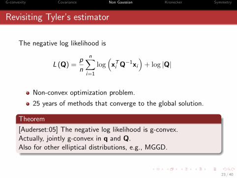
Revisiting Tyler’s estimator

The negative log likelihood is

L (Q) =p

n

n∑

i=1

log(xTi Q

−1xi)

+ log |Q|

Non-convex optimization problem.

25 years of methods that converge to the global solution.

Theorem

[Auderset:05] The negative log likelihood is g-convex.Actually, jointly g-convex in q and Q.Also for other elliptical distributions, e.g., MGGD.

23 / 40


Why is this helpful? Regularization

Often, we need regularization / prior.

[Abramovich:07], [Chen:10] difficult design and analysis.

We propose to use g-convex regularization schemes

Global solution to ML (+ regularization)

min L (·) + λh(·)︸︷︷︸needs to be g-convex

Guaranteed to be g-convex, and can be solved efficiently. We canput priors on both the covariance and the scalings.

24 / 40


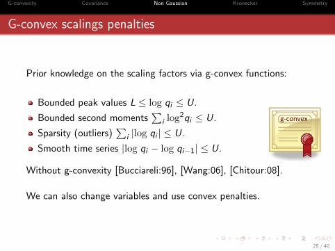
G-convex scalings penalties

Prior knowledge on the scaling factors via g-convex functions:

Bounded peak values L ≤ log qi ≤ U.

Bounded second moments∑

i log2qi ≤ U.

Sparsity (outliers)∑

i |log qi | ≤ U.

Smooth time series |log qi − log qi−1| ≤ U.

g"convex)

Without g-convexity [Bucciareli:96], [Wang:06], [Chitour:08].

We can also change variables and use convex penalties.

25 / 40


G-convex matrix penalties

Shrinkage to identity (T = I) or arbitrary target

h (Q) = plog(Tr{Q−1T

})+ log |Q|

Shrinkage to diagonal

h (Q) = log

p∏

i=1

[Q−1

]ii

+ log |Q|

Regularization of condition number

h (Q) =λmax (Q)

λmin (Q)

g"convex)

Non-Gaussian versions of [Stoica:08], [Schafer:05], [Won:09].

26 / 40


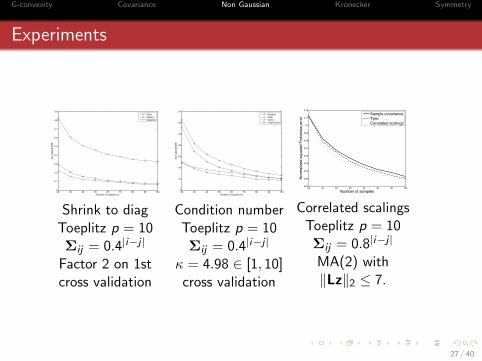
Experiments

20 30 40 50 60 70 80 90 1000

0.1

0.2

0.3

0.4

0.5

0.6

0.7

0.8

0.9

Number of samples (n)

Nor

mal

ized

MSE

TylerIdentityDiagonal

Shrink to diagToeplitz p = 10Σij = 0.4|i−j |

Factor 2 on 1stcross validation

20 30 40 50 60 70 80 90 1000

0.1

0.2

0.3

0.4

0.5

0.6

0.7

Number of samples (n)

Nor

mal

ized

MSE

SampleTylerCondTyler+Cond

Condition numberToeplitz p = 10Σij = 0.4|i−j |

κ = 4.98 ∈ [1, 10]cross validation

30 40 50 60 70 80 90 1000.02

0.03

0.04

0.05

0.06

0.07

0.08

0.09

0.1

0.11

0.12

Number of samples

Nor

mal

ized

squ

ared

Fro

beni

us e

rror

Sample covarianceTylerCorrelated scalings

Correlated scalingsToeplitz p = 10Σij = 0.8|i−j |

MA(2) with‖Lz‖2 ≤ 7.

27 / 40


Outline



3 Non Gaussian

4 Kronecker models


28 / 40


Kronecker (separable, transposable) model Q1 ⊗Q2

Estimating covariances of random p2 × p1 matrices.

A standard approach is to impose structure

X = Q122WQ

121

Wij are i.i.d. N (0, 1).Q2 correlates the columns.Q1 correlates the rows.

In vector notations, E[xxT

]= Q1 ⊗Q2

Examples: Tx ⊗ Rx, products ⊗ costumers, etc...

29 / 40


A bit of background Q1 ⊗Q2

[Mardia:93], [Dutilleul:99] Introduction, Flip-Flop.

[Kermoal:02] Experiments in MIMO radio channels.

[Lu:05], [Srivastava:08] Testing, uniqueness.

[Werner:08] Asymptotic analysis and extensions.

[Allen:10] Regularization and applications in bioinformatics.

[Zhang:10], [Stegle:11] Sparsity, multitask learning.

[Tsiligkaridis:12] COMING UP COLLOQUIUM.

[Akdemir:11] Multiway Kronecker models.

Lots of applications! Lots of difficult theory!But specific and hard to follow and generalize.

30 / 40


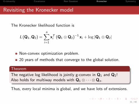
Revisiting the Kronecker model

The Kronecker likelihood function is

L (Q1,Q2) =n∑

i=1

xTi (Q1 ⊗Q2)−1 xi + log |Q1 ⊗Q2|

Non-convex optimization problem.

20 years of methods that converge to the global solution.

Theorem

The negative log likelihood is jointly g-convex in Q1 and Q2!Also holds for multiway models with Q1 ⊗ · · · ⊗Qn.

Thus, every local minima is global, and we have lots of extensions.

31 / 40


Why is this helpful? Regularized ML

Kronecker models do not require many samples.

[Allen:10] one sample + regularization via SVD.We propose

minQ1,Q2

L (Q1,Q2) + αTr{Q−11

}Tr{Q−12

}

which is jointly g-convex.

p1 = p2 = 5Σij = 0.8|i−j |

0 2 4 6 8 10 12 14 16 18 200

0.05

0.1

0.15

0.2

0.25

0.3

0.35

0.4

0.45

0.5

Number of samples

Nor

mal

ized

squ

ared

Fro

beni

us e

rror

SampleFPIRFPI 0.01RFPI 0.03

32 / 40


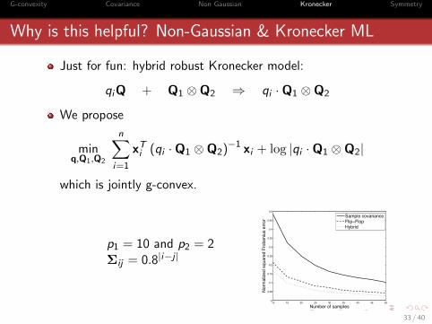
Why is this helpful? Non-Gaussian & Kronecker ML

Just for fun: hybrid robust Kronecker model:

qiQ + Q1 ⊗Q2 ⇒ qi ·Q1 ⊗Q2

We propose

minq,Q1,Q2

n∑

i=1

xTi (qi ·Q1 ⊗Q2)−1 xi + log |qi ·Q1 ⊗Q2|

which is jointly g-convex.

p1 = 10 and p2 = 2Σij = 0.8|i−j |

10 15 20 25 30 35 40 45 500

0.05

0.1

0.15

0.2

0.25

0.3

0.35

0.4

0.45

0.5

Number of samples

Nor

mal

ized

squ

ared

Fro

beni

us e

rror

Sample covarianceFlip−FlopHybrid

33 / 40


Outline



3 Non Gaussian

4 Kronecker models


34 / 40


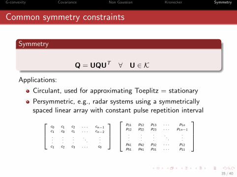
Common symmetry constraints

Symmetry

Q = UQUT ∀ U ∈ K

Applications:

Circulant, used for approximating Toeplitz = stationary

Persymmetric, e.g., radar systems using a symmetricallyspaced linear array with constant pulse repetition interval

c0 c1 c2 . . . cn−1c1 c0 c1 . . . cn−2

.

.

.

.

.

.

.

.

.. . .

.

.

.c1 c2 c3 . . . c0

p11 p12 p13 . . . p1np12 p22 p23 . . . p1n−1

.

.

.

.

.

.

.

.

.. . .

.

.

.p41 p42 p32 . . . p12p51 p41 p31 . . . p11

35 / 40


More symmetry constraints - properness

Symmetry

Q = UQUT ∀ U ∈ K

Applications:

Complex normal = double real normal (CN p = N2p)

Plus a symmetry constraint x ∼ e jθx.

cov

[Re (x)Im (x)

]=

[A B−B A

]

Recently, proper Gaussian quaternions x = a + ib + jc + kd.

For example, in radar with I/Q phase and polarizations

Here too: QN p = N4p + special symmetry x ∼ eνθx.

36 / 40


A bit of background Q = UQUT

Gaussian

Genreal symmetry groups [Shah & Chandrasekaran 2012]Everybody knows proper complex (circularly symmetric)Proper quaternion [Miron:06], [Bukhari:11], [Via:11]....

Non Gaussian

Persymmetric [Pailloux:11]Complex elliptical distributions [Bombrun:11], [Ollila:12]

Lots of applications! But specific and hard to follow and generalize.Easy in the Gaussian case (linear constraint).

37 / 40


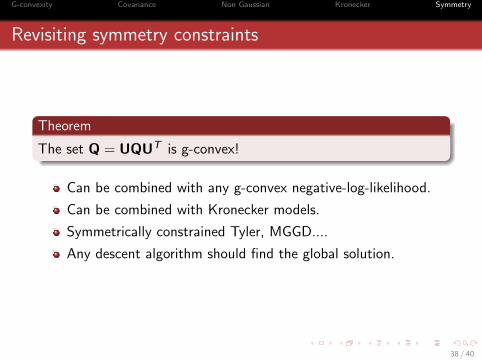
Revisiting symmetry constraints

Theorem

The set Q = UQUT is g-convex!

Can be combined with any g-convex negative-log-likelihood.

Can be combined with Kronecker models.

Symmetrically constrained Tyler, MGGD....

Any descent algorithm should find the global solution.

38 / 40


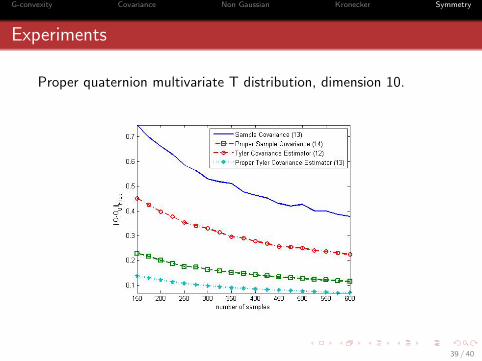
Experiments

Proper quaternion multivariate T distribution, dimension 10.

4

VI. NUMERICAL RESULTS

For numerical simulations, we chose Tyler’s scatter esti-mate in proper quaternion distributions. We have generated aproper real covariance matrix Q0 and generated ellipticallydistributed 10-dimensional quaternion random vectors assi =

p⌧v, where ⌧ ⇠ �2 and v is zero-mean normally

distributed with covariance matrix Q0. We choose ⇢(x) =plog(x) to get the Tyler’s covariance estimator [10].

We compare four different covariance estimators:

• Sample Covariance

QSC =1

n

nX

i=1

sisTi , (11)

• Proper Sample Covariance

QPSC =1

|K|nX

Ł2K

nX

i=1

ŁsisTi ŁT , (12)

• Tyler Covariance Estimator Iteration

Qk+1 =p

n

nX

i=1

sisTi

sTi Q�1

k si

. (13)

• Tyler Proper Covariance Estimator Iteration

Qk+1 =p

|K|nX

Ł2K

nX

i=1

ŁsisTi ŁT

sTi ŁT Q�1

k Lsi

=p

|K|nX

Ł2K

nX

i=1

(Łsi)(Łsi)T

(Łsi)T Q�1k (Łsi)

.

(14)

We repeat the computations for 100 times for the fourestimators with 150 � 600 samples. In order to make theresults consistent we divide all the matrices by their traces.

VII. ACKNOWLEDGEMENT

This work was partially supported by Israel Science Foun-dation Grant No. 786/11 and Kaete Klausner Scholarship.The authors would like to thank Alba Sloin for numerousand helpful discussions.

REFERENCES

[1] Krim H., Viberg M., Two decades of array signal processing research:The parametric approach, IEEE Signal Process. Mag., vol. 13, no. 4,pp. 6794, July 1996.

[2] Dougherty E. R., Datta A., Sima C., Research issues in genomicsignal processing, IEEE Signal Process. Mag., vol. 22, no. 6, pp.4668, November 2005.

[3] Abramovich Y. I., Spencer N. K., Diagonally loaded normalisedsample matrix inversion (LNSMI) for outlier-resistant adaptive filter-ing, IEEE International Conference on Acoustics, Speech and SignalProcessing, ICASSP, vol. 3, 2007.

[4] Bandiera F., Besson O., Ricci G., Knowledge-aided covariance matrixestimation and adaptive detection in compound-Gaussian noise, IEEETransaction on Signal Processing, vol. 58, no. 10, pp. 53915396, 2010.

[5] Chen Y., Wiesel A., Hero A. O., Robust shrinkage estimation ofhigh-dimensional covariance matrices, IEEE Transactions on SignalProcessing, vol. 59, no. 9, pp. 40974107, 2011.

[6] Wiesel A., Unified framework to regularized covariance estimationin scaled Gaussian models, IEEE Transactions on Signal Processing,vol. 60, no. 1, pp. 29 38, 2012.

[7] Wiesel A., Regularized covariance estimation in scaled gaussianmodels, 4th IEEE International Workshop on Computational Advancesin Multi-Sensor Adaptive Processing (CAMSAP) pp. 309312, 2011.

[8] Zhang T., Wiesel A., Greco M. S., Multivariate General-ized Gaussian Distribution: Convexity and Graphical Models,http://arxiv.org/pdf/1304.3206.pdf.

[9] Shah P., Chandrasekaran V., Group Symmetry and Covariance Reg-ularization, Electronic Journal of Statistics, vol. 6, pp. 1600-1640,2012.

[10] Tyler D. E., A distribution-free M-estimator of multivariate scatter,The Annals of Statistics, vol. 15, no. 1, pp. 234-251, 1987.

[11] Ramrez D. J. Via, Santamara I., Properness and widely linear pro-cessing of quaternion random vectors, IEEE Transactions on SignalProcessing, vol. 56, no. 7, pp. 3502-3515, 2010.

[12] Pascal F., Chitour Y., Ovarlez J.-F., Forster P., Larzabal P., CovarianceStructure Maximum-Likelihood Estimates in Compound GaussianNoise: Existence and Algorithm Analysis, IEEE Transactions onSignal Processing, vol. 56, no. 1, January 2008.

[13] Wiesel A., Geodesic convexity and covariance estimation, IEEETransactions on Signal Processing, vol. 60, no. 12, January 2012.

[14] Kay S. M., Fundamentals of Statistical Signal Processing: EstimationTheory, Volume 1, Prentice-Hall PTR, 1998.

[15] Maximum likelihood estimation of structured persymmetric covariancematrices, Signal Processing Volume 83, Issue 3, Pages 633640, March2003,

[16] Pailloux G., Forster P., Ovatlez J.-P., Pascal F., Persymmetric AdaptiveRadar Detectors, IEEE Transactions on Aerospace and ElectronicSystems, vol. 47, no. 4, pp. 2376-2389, October 2011.

[17] Dembo A., Mallows C. L., Shepp L. A., Embedding NonnegativeDefinite Toeplitz Matrices in Nonnegative Definite Circulant Matrices,with Application to Covariance Estimation, IEEE Transactions onInformation Theory, vol. 35, no. 6, pp. 2376-2389, November 1989.

[18] Rapcsak T., Geodesic convexity in nonlinear optimization, Journal ofOptimization Theory and Applications, vol. 69, pp. 169-183, 1991.

[19] Cai T. T., Ren Z., Zhou H. H., Optimal Rates ofConvergence for Estimating Toeplitz Covariance Matrices,http://www.stat.yale.edu/⇠hz68/Toeplitz.pdf

[20] Frahm G., Generalized Elliptical Distributions: Theory and Applica-tions, PhD thesis, Univesity of Keln, 2004.

[21] Chen Y., Wiesel A., Hero A. O., Robust Shrinkage Estimation of High-dimensional Covariance Matrices, http://arxiv.org/pdf/1009.5331.pdf

[22] Bickel P. J., Levina E., Regularized Estimation of Large CovarianceMatrices, Annals of Statistics, vol. 36, no. 1, pp. 199227, 2008.

[23] Sloin A. Wiesel A., Proper Quaternion Gaussian Graphical Models,in preparation.

[24] Ollila E., Tyler D. E., Koivunen, V., Poor H. V., Complex EllipticallySymmetric Distributions: Survey, New Results and Applications, IEEETransactions on Signal Processing, vol. 60, no. 11, pp. 5597-5625,November 2010.

[25] Ollila E., Tyler D. E., Distribution-free detection under complexelliptically symmetric clutter distribution, IEEE 7th Sensor Array andMultichannel Signal Processing Workshop (SAM), 2012.

[26] Miron S., Le Bihan N., Mars J. I., Quaternion-MUSIC foe Vector-Sensor Array Processing, IEEE Transactions on Signal Processing,vol. 56, no. 7, pp. 1218-1229, April 2006.

39 / 40


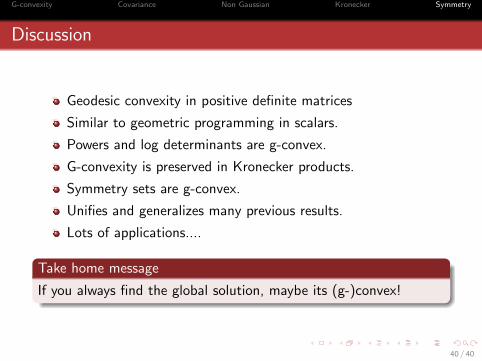
Discussion

Geodesic convexity in positive definite matrices

Similar to geometric programming in scalars.

Powers and log determinants are g-convex.

G-convexity is preserved in Kronecker products.

Symmetry sets are g-convex.

Unifies and generalizes many previous results.

Lots of applications....

Take home message

If you always find the global solution, maybe its (g-)convex!

40 / 40

Geodesic convexity & covariance estimation - IRIT · based power control for general SIR regime. In...

Documents

Transcript of Geodesic convexity & covariance estimation - IRIT · based power control for general SIR regime. In...