University of Rhode Island University of Rhode Island

DigitalCommons@URI DigitalCommons@URI

Open Access Master's Theses

2018

GEOCHEMISTRY OF HIGHLY ALKALINE WATERS OF THE COAST GEOCHEMISTRY OF HIGHLY ALKALINE WATERS OF THE COAST

RANGE OPHIOLITE IN CALIFORNIA, USA RANGE OPHIOLITE IN CALIFORNIA, USA

Mahrukh Shaikh University of Rhode Island, mahrukh79@gmail.com

Follow this and additional works at: https://digitalcommons.uri.edu/theses

Recommended Citation Recommended Citation Shaikh, Mahrukh, "GEOCHEMISTRY OF HIGHLY ALKALINE WATERS OF THE COAST RANGE OPHIOLITE IN CALIFORNIA, USA" (2018). Open Access Master's Theses. Paper 1310. https://digitalcommons.uri.edu/theses/1310

This Thesis is brought to you for free and open access by DigitalCommons@URI. It has been accepted for inclusion in Open Access Master's Theses by an authorized administrator of DigitalCommons@URI. For more information, please contact digitalcommons@etal.uri.edu.

GEOCHEMISTRY OF HIGHLY ALKALINE WATERS

OF THE COAST RANGE OPHIOLITE

IN CALIFORNIA, USA

BY

MAHRUKH ANWAR

A THESIS SUBMITTED IN PARTIAL FULFILLMENT OF THE

REQUIREMENTS FOR THE DEGREE OF

MASTER OF SCIENCE

IN

BIOLOGICAL AND ENVIRONMENTAL SCIENCES

UNIVERSITY OF RHODE ISLAND

2018

MASTER OF SCIENCE IN BIOLOGICAL AND ENVIRONMENTAL SCIENCES

OF

MAHRUKH ANWAR

APPROVED:

Thesis Committee:

Major Professor Dawn Cardace

Ali Akanda

Soni Pradhanang

Nasser H. Zawia

DEAN OF THE GRADUATE SCHOOL

UNIVERSITY OF RHODE ISLAND

2018

ABSTRACT

Altered waters impacted by serpentinization of Coast Range Ophiolite (CRO)

ultramafic units have been reacting with trapped Cretaceous seawaters, meteoric

waters, and other surface derived waters since tectonic emplacement of this ophiolite.

In 2011, groundwater monitoring wells of various depths were established near Lower

Lake, CA, USA in the McLaughlin Natural Reserve, administered by the University of

California-Davis, in order to understand ongoing low temperature alterations and

biogeochemical interactions taking place. Wells were installed at two sites in the

Reserve. There are three Quarry Valley area wells (QV1-1 [23m depth], QV1-2

[14.9m], QV1-3 [34.6m]) and five Core Shed area wells (CSW1-1 [19.5m], CSW1-2

[19.2m], CSW1-3 [23.2m], CSW1-4 [8.8m], CSW1-5 [27.4m]). Water samples were

collected from all installed wells, as well as from an older well drilled near the historic

core shed (Old Core Shed Well, or OCSW [82m]), and an upper (TC1) and lower

(TC2) site sampling a nearby groundwater-fed alkaline seep, at Temptation Creek.

Key environmental parameters (temperature, pH, conductivity, oxidation-reduction

potential, and dissolved oxygen) were collected in the field using YSI-556 multiprobe

meter, and total concentrations for major cations (Ca+2, Na+, Mg+2, K+) were analyzed

using Thermo Scientific iCAP 7400 Inductively Coupled Plasma-Atomic Emission

Spectrometry, and anions (F-, Cl-, SO4-2, NO3

-) on Dionex Modular DX 500 Ion

Chromatography.

Principal component analysis was conducted to determine key factors and

processes controlling water chemistries at CRO. Geochemist’s Workbench software

was used to model the low temperature alteration of a serpentinization-influenced

model water volume passing through serpentinite over a period of 100 million years.

Modeling provided insight into the changing pH, Eh, evolving water chemistries,

stepwise mineral assemblages, appearance of marker minerals at geochemical

transitions in the system, and supported evidence of pervasive impacts of low

temperature, oxidative weathering of serpentinites. This work supports the case of

incremental dilution and transformation of a deeply sourced Ca2+-OH- Type II water in

this environment, and constrains reaction status of present day CRO waters and those

of similar sites, in terms of the progress of serpentinite weathering reactions. Further,

the study informs our understanding of serpentinization-related geological

environments present on other celestial bodies (e.g., Mars, Europa, Enceladus) in our

Solar System and beyond.

iv

ACKNOWLEDGMENTS

It is not very often that we come across people who go above and beyond to

help, reach out and support in every way possible. For me, it has been Dr. Dawn

Cardace. She was my mentor the day I started my undergraduate studies at the

Department of Geosciences, at the University of Rhode Island. I had no idea then that

I would have the good fortune of returning back for a master’s program under Dr.

Cardace caring mentorship. She has been my guiding light, my anchor, and my rock

for all these years at URI. I can never thank her enough for all that she did for me.

I would also like to thank my thesis committee, Dr. Ali Akanda and Dr. Soni

Pradhanang, and my defense chair Dr. Alison Tovar, and my Geology Department

professors: Dr. Boving, Dr. Engelhart, Dr. Fastovsky, Dr. Laliberte, Dr. Pradhanang,

Dr. Savage, and Dr. Veeger. A special thank you to Julie Smallridge, and Ken

Wilkinson. I would also like to thank all my departmental colleagues, especially

Khurshid, Michaela, Reilly, and Jordanne.

Alex, Marzia, Jeeban: thank you for being wonderful officemates. I enjoyed

every minute I got to spend with you all in our tiny yet welcoming office.

Roger: thank you for always checking on how I am doing, for always encouraging,

and for the big smiles and hugs, and last but not least, our mutual love of anything

automobile-related.

Alex: I have lost count of the number of times you ran to print pages for me on a

minute’s notice for our meetings. Thank you for everything you have done, including

helping with the move and for sharing Trevor Noah You-Tube clips.

v

Meg: you were like a sister for me from the first day we met. From stickers, museum

tickets, delicious home cooked meals, you were always there to hug me and tell me

“Mahrukh, it will be okay!” And it was.

Alex, Meg, Roger: I will miss all the times we spent together gathered around the big

table for our meetings with Dr. Cardace.

I would like to acknowledge and thank my loving and supportive family for

not letting me give-up, for supporting me through all these years, and for being there

for me through thick and thin. Mom and dad, my siblings Naushin, Khurram, and

Sania, brothers in laws Naeem and Nabeel, and my nephew and niece Ayman, and

Asra. Thank you all so much!

To my daughters, Aiza and Rania: I love you both more than words can

describe. Thank you for understanding all the times you both endured my submission

deadlines and finals, for never complaining about me not being able to spend more

family time and weekends out of the house. Rania, thank you for accompanying me to

my college all these years and attending the classes with me since you were five years

old. Aiza, I cannot forget all the times you spent in the lab with me patiently waiting

for me to finish my work so we could go home.

I would also like to recognize the support and funding from the University of

Rhode Island, College of Environmental and Life Sciences for teaching assistantship,

NASA Astrobiology Institute CAN7 Rock Powered Life Award to Co-Investigator

Cardace (Solicitation # NNH13ZDA017C), and NASA Rhode Island Space Grant

College and Fellowship Program, Space Grant Opportunities in NASA STEM

vi

(Solicitation #NNX15AI06H). I would also like to thank Joseph Orchardo for helping

with the use of equipment necessary for this research at Brown University.

vii

PREFACE

This document is prepared in manuscript format and adheres to the style of the

scientific journal Chemical Geology.

viii

TABLE OF CONTENTS

ABSTRACT ................................................................................................................... ii

ACKNOWLEDGMENTS ............................................................................................ iv

PREFACE .................................................................................................................... vii

TABLE OF CONTENTS ............................................................................................ viii

LIST OF TABLES ........................................................................................................ ix

LIST OF FIGURES ....................................................................................................... x

MANUSCRIPT INTRODUCTORY PAGE. ................................................................. 1

INTRODUCTION ......................................................................................................... 2

GEOLOGIC SETTING .................................................................................................. 7

ANALYTICAL METHODS ........................................................................................ 10

RESULTS .................................................................................................................... 17

DISCUSSION .............................................................................................................. 28

CONCLUSION AND FUTURE WORK SUGGESTIONS ........................................ 33

REFERENCES………………………………………………………………………..34

APPENDICIES……………………………………………………………………….75

ix

LIST OF TABLES

TABLE PAGE

Table 1. The inputs used in GWB modeling. .............................................................. 69

Table 2. Ionic composition of regional precipitation at Menlo Park, California. ....... 70

Table 3. Ionic composition of seawater. ..................................................................... 71

Table 4. Field data collected in 2017 .......................................................................... 72

Table 5. Ionic Composition of the CROMO samples from 2017 ............................... 73

Table 6. Principal components analysis data table...................................................... 74

Table A-1. Making dilutions for IC calibrations using the Standard Stock Solutions 76

Table A-2. Sample dilution protocol ………………………………………………. 77

x

LIST OF FIGURES

FIGURE PAGE

Figure 1. Geologic map of the Coast Range, with the ophiolite exposures in solid

black, and the star indicating the location of McLaughlin Natural Reserve in Western

California……………………………………………………………………………. 39

Figure 2. Global distribution of ophiolites, except Spain, Japan (peridotite massifs)

and Portugal (peridotite intrusion).…………………………………………………. 40

Figure 3. Aerial map of the three main sampling locations from McLaughlin Reserve

created in Google Earth……………………………………………………………....41

Figure 4. The conceptual model of the REACT mode simulation…………………. 42

Figure 5. Depth profile of the wells at McLaughlin Natural Reserve, California…... 43

Figure 6. Calcium to magnesium ratios plot………………………………………… 44

Figure 7. Ca+2 and Mg+2 ionic composition of CRO samples……………………….. 45

Figure 8. Na+ and Cl- ionic composition of CRO samples…………………………...46

Figure 9. XY plot of sodium and chloride ion concentrations………………………. 47

Figure 10. Electrical conductivity of the CRO samples………………………………48

Figure 11. Eh-pH plot for CRO samples……………………………………………...49

Figure 12. Electrical conductivity (as a proxy for total dissolved solids) and ionic

concentrations of samples…………………………………………………………….50

Figure 13. Stiff diagrams of major ionic makeup for CRO

samples……………………………………………………………………………….51

Figure 14. Ionic makeup of the 2017 CRO waters………………………………….. 52

Figure 15. Principal components analysis results with Eigenvalue Pareto Plot, Score

xi

Plot, and Loading Plot………………………………………………………………...53

Figure 16. GWB REACT mode simulation for changing pH over the course of 100

million years at 250C………………………………………………………………….54

Figure 17. GWB REACT mode simulation for changing pH over the course of 100

million years at 1000C. ……………………………………………………………….55

Figure 18. GWB REACT mode simulation for changing pH over the course of 100

million years at 20C. ………………………………………………………………….56

Figure 19. GWB REACT mode simulation for changing Eh (mV) over the course of

100 million years at 250C. ……………………………………………………………57

Figure 20. GWB REACT mode simulation for changing Eh (mV) over the course of

100 million years at 1000C. …………………………………………………………. 58

Figure 21. GWB REACT mode simulation for changing Eh (mV) over the course of

100 million years at 20C. ……………………………………………………………. 59

Figure 22. GWB REACT mode simulation for changing fluid chemistries (mg/kg)

over the course of 100 million years at 250C…………………………………………60

Figure 23. GWB REACT mode simulation for changing fluid chemistries (mg/kg)

over the course of 100 million years at 1000C………………………………………. 61

Figure 24. GWB REACT mode simulation for changing fluid chemistries (mg/kg)

over the course of 100 million years at 20C…………………………………………. 62

Figure 25. GWB REACT mode simulation for changing mineralogy (volume%) over

the course of 100 million years at 250C………………………………………………63

Figure 26. GWB REACT mode simulation for changing mineralogy (volume%) over

the course of 100 million years at 1000C……………………………………………. 64

xii

Figure 27. GWB REACT mode simulation for changing mineralogy (volume%) over

the course of 100 million years at 20C………………………………………………. 65

Figure 28. Classification of water samples based upon the Ca/Mg ratios……………66

Figure 29. Classification of water samples based upon Eh-pH………………………67

Figure 30. Summary of bedrock-water interactions taking place at the Coast Range

ophiolite, as a framework for grouping CRO waters…………………………………68

1

MANUSCRIPT

This manuscript is prepared for submission to the Chemical Geology.

2

INTRODUCTION

The Coast Range Ophiolite (CRO) is a tectonized mélange of units of the

oceanic lithosphere, stretching north of San Francisco area in California, U.S.A.

(Cardace et al., 2013). Here, the Middle to Late Jurassic CRO exposures represent

deformed and structurally dismembered segments of oceanic crust and uppermost

mantle, now incorporated within the continental block (Dickinson et al., 1996), that

are undergoing a unique process of long-term aqueous alteration, characterized as

vigorous serpentinization (Figure 1) followed by low temperature, oxidative

weathering.

Serpentinization is the process during which ultramafic mantle rocks rich in

olivine and pyroxene react with water, leading to formation of serpentinite rock that is

dominated by serpentine group minerals including lizardite, chrysotile and antigorite

(Moody, 1976). This water-rock reaction is accompanied by the generation of fluids

with high concentrations of hydrogen (Corliss et al. 1981; Russell, 2007; Ehlmann et

al, 2010), increase in rock volume, and release of heat energy (Allen and Seyfried,

2004). Serpentinization can be summarized as:

olivine + water → serpentine + brucite + magnetite

(Mg,Fe)2SiO4 + H2O → (Mg,Fe)3Si2O5(OH)4 + (Mg,Fe)(OH)2 + Fe3O4 + H2

2(FeO) rock + H2O → (Fe2O3) rock + H2

Here, the parent mineral olivine, containing magnesium, iron, silicon, and

oxygen, reacts with H2O resulting in the oxidation of iron from ferrous ions (Fe+2) to

ferric ions (Fe+3), while the water molecules are reduced to hydrogen gas and

3

hydroxide ions (OH-). These OH- ions drive the pH of the serpentinizing waters to

high alkaline levels. Coast Range Ophiolite is one of the rare, well documented sites

where these hyperalkaline waters exist (Figure 2).

The process of serpentinization has recently gained attention due to the

production of highly reducing environments enriched in molecular hydrogen and

methane, all of which can provide microbial communities with chemical energy that

can sustain biomass--providing favorable living conditions within the deep biosphere.

Life support by chemical energy instead of photosynthesis has provided prospects for

life’s existence on other celestial bodies like Mars and Jupiter’s moon Europa

(McCollom et al., 2013). The characteristic mineralogy and aqueous geochemistry at

Earth-based serpentinizing sites are analogous to subsurface Martian environments,

where the altered olivine-rich rocks (olivine detections, Koeppen et al. 2008,

serpentine detections, Ehlmann et al., 2010) suggest occurrence of serpentinization in

past. In fact, serpentinization may be ongoing in the subsurface, with some evidence

for continuing groundwater flow (Michalski et al., 2013), conveniently sheltered from

sterilization by incoming cosmic radiation on the surface of Mars (Zeitlin et al., 2004).

Simultaneously, this ability of microorganisms to survive also provides explanation

and insight into synthesis of organic compounds needed in the origination of life on

Earth (Lang et al., 2010, Martin et al., 2008).

Another important area of significance and ongoing research involves

serpentinization for its role in carbon sequestration (carbon capture and storage, CCS).

The hyperalkaline serpentinizing waters contain almost no dissolved inorganic carbon

(DIC). When these waters reach the surface or get discharged, atmospheric carbon

4

dioxide is rapidly taken up and converted into insoluble carbonates (Burns & Matter,

1995; Chizmeshya et al., 2007; Andreani et al., 2009; Kelemen et al., 2011; Paukert et

al., 2012). This presents a way to store the increasing and alarming concentrations of

carbon dioxide from the atmosphere and is now an active area of ongoing research

with a promising potential of reversing the effects of anthropogenic global warming

(McCollom et al., 2013).

Given these recent scientific research interest in serpentinites, the objective of

this paper is to develop a more thorough understanding of the serpentinite weathering,

geochemistry of the serpentinizing fluids, serpentinite rock-water interactions, and

changes in mineralogy and fluids chemistry with the passage of time.

The interaction of the serpentines with water and causing the resulting waters

to undergo unique chemical changes was first reported and studied by Barnes and

colleagues in 1967. Barnes compared the ionic concentrations of the unusual

ultrabasic spring samples from Red Mountain in California, John Day in Oregon, and

Cazadero in California, and proposed that these unusual waters were genetically

related to serpentinization (Barnes et al., 1967). Later, in 1977, Barnes and O’Neil

compared the pH, ionic makeup, and other compositional properties of the water

samples collected from the serpentinizing sites in New Caledonia and Yugoslavia and

compared those with the samples from Oman (collected by Bailey and Coleman), and

the samples from Oregon and California. Barnes and O’Neil found the water

composition of all these sites to be similar in composition and reaction pathways for

low-temperature based serpentinization rock-water reactions (Barnes & O’Neil, 1977).

In 2012, Paukert et al., characterized the ionic makeup of spring and well water

5

samples from Samail ophiolite using ion chromatography (IC) on a Dionex 2000 with

an AS18 column for the anions, and inductively coupled plasma atomic emission

spectrometry (ICP-AES) with Horiba Jobin-Yvon Activa M with PFA nebulizer for

the cations (Paukert et al., 2012). The resulting geochemistry of waters were classified

as being of two different types: those that were high in the Mg2+ and -HCO3- (named

Type I waters), and those with high Ca+2 and -OH- (named Type II waters).

The serpentine soils are unique as they are naturally deprived in nutrients that

plants need; instead they are rich in Mg, Fe, and trace elements that include Ni, Cr,

Cd, Co, Cu, and Mn (Wildman et al., 1968, D’Amico & Previtali, 2012). This creates

a challenging environment for plants to grow in. The serpentine endemic species are

visibly different from other plants growing in a landscape with serpentine soil

exposures and have evolved and shown adaptations that fit this unique environment

(Safford et al., 2005; Alexander, 2007). Due to their harsh nature, the serpentine soils

at Coast Range locale and other similar sites have been studied from an ecological

point of view. How they weather under natural environments is little studied as yet.

Also, the weathering processes tend to differ site to site due to differences in

topography, parent rock mineralogy, climate and rainfall.

It is proposed that CRO is a site of on-going low temperature serpentinization

leading to production of different fluids that are reflective of rock-water interactions.

A reaction pathway can be modeled to explain the temporal changes in mineralogy

and fluid chemistries. To confirm this, water samples were collected from Coast

Range ophiolite, McLaughlin Natural Reserve area. The key environmental

parameters were recorded onsite and the ionic makeup of the waters were determined

6

using ion chromatography (IC) for the concentrations of major anions (F-, Cl-, SO4-2,

NO3-), and Inductively Coupled Plasma Atomic Emission Spectrometer system (ICP-

AES) for major cations (Ca+2, Na+, Mg+2, K+). The ionic data were quantified and

analyzed. JMP Statistical Data Analysis Software was used for principal components

analysis (PCA) to explain key factors and processes controlling the water chemistries

at CRO. X-ray diffraction (XRD) data from CRO well cores and ionic make up of four

types of waters (local meteoric water, seawater, a 10% dilute seawater, and an

ultrabasic groundwater solution) were added as an input in Geochemist’s Workbench

(GWB) software to model the evolving water chemistry, mineralogy, pH and Eh

changes. As the terrestrial sites of serpentinization experience low temperature,

relatively oxidizing weathering near the planetary surface, the aqueous geochemistry

of waters and the corresponding mineral lithologies evolve and provide insight into the

complex rock-water interactions.

7

GEOLOGIC SETTING

During the Jurassic and Cretaceous periods, the oceanic Farallon Plate, moving

west, collided with the North American continental margin and underwent subduction.

This subduction lead to the formation of the Coast Ranges and Sierra Nevada on the

west coast of United States. With time, the scraping off of material from the down-

going Farallon plate formed an accretionary wedge, known now as the Franciscan

mélange (French for “mixture”), and the weathering of the Sierra Nevada settled in the

ocean basin just beyond the tip of continent and became known as the Great Valley

Sequence. Later, complex folding and faulting events between the two plates exposed

a piece of the Middle Jurassic oceanic crust and mantle (ophiolite) named Coast Range

Ophiolite, which has the Great Valley Sequence on the east, and the Franciscan

complex on the west. The Coast Range Ophiolite consists largely of serpentinite,

partly serpentinized peridotite, gabbro, and basalt (University of California, 2003).

8

FIELD SITE

About 600 km north of the Golden Gate Bridge is one block of the Coast

Range Ophiolite, in the McLaughlin Natural Reserve, near the junction of Napa, Lake,

and Yolo Counties. This unique geologic area of 6,940 acres is managed by the

University of California to protect and conduct research in the unusual serpentine-rich

habitats. In 2011, eight monitoring wells were installed, funded by the NASA

Astrobiology Institute, in ultramafic units rich in serpentine minerals, derived from the

regionally important convergent margin mélange environment. The CRO monitoring

wells at the McLaughlin Natural Reserve provide a means to sample periodically the

formation waters moving through a shallowly emplaced ultramafic unit, with

logistically simple access.

Climate

The reserve receives an average precipitation of 75.7 cm per year, with the

average temperatures of July as 24.6 ºC and January’s average temperature of 7.3 ºC

(Natural Reserve System University of California, 2018). Regional climate is

Mediterranean-type, with summers being dry and hot, and winters wet and cold

(Mathany & Belitz, 2015).

Hydrogeology

The movement of groundwater follows the area’s topography and the direction

of flow of the surface water features. The recharge to groundwater is primarily

through the precipitation and runoff from surface water features (Mathany & Belitz,

2015).

9

Sampling Locations

Eight monitoring wells were installed near Lower Lake, CA, in the McLaughlin

Natural Reserve. Wells were installed at two sites in the Reserve, namely the Quarry

Valley and the Core Shed. These wells are designated (bottom of hole depth in meters

provided in brackets after well ID): QV1-1 [23 m], QV1-2 [14.9 m], QV1-3 [34.6 m],

CSW1-1 [19.5 m], CSW1-2 [19.2 m], CSW1-3 [23.2 m], CSW1-4 [8.8 m], CSW1-5

[27.4 m]. An old well known as Old Core Shed well, OCSW [82 m] is present near the

Core Shed wells. This deep well was already present on site before the other wells

were drilled. The main well for Core Shed wells is the CSW1-1, with the other Core

Shed wells located within 5m of CSW1-1. The main well for the Quarry Valley wells

is the QV1-1, with the other Quarry Valley wells present within 3m of QV1-1. Each

well reaches a different depth in the shallow subsurface.

The two other sampling sites (TC1 and TC2) include an upstream and

downstream point along a seasonally active ground-water fed creek, the Temptation

Creek (TC). TC1 is the area where the groundwater seep is emerging from, and TC2 is

the percolating water before it disperses into the landscape. The distance between TC1

and TC2 is about 515m with a relief of 65m (Figure 3).

10

ANALYTICAL METHODS

Field Methods

Collection of Water Samples

Water samples were collected during the months of May and June of 2016 and

of 2017. The sampling sites included the 8 groundwater wells (CSW1-1, CSW1-2,

CSW1-3, CSW1-4, CSW1-5), the Old Core Shed well (OCSW), and two surface

water sites, Temptation Creek 1 (TC1) and Temptation Creek 2 (TC2).

Samples were collected via syringes (rinsed three times) fitted with 0.22 µm pore size

filters. No pretreatment was required for IC samples, which were stored in clean,

plastic laboratory bottles and frozen until analysis. The samples for ICP-AES were

collected in certified 100 ml Nalgene bottles, spiked with 70% trace metal grade

HNO3, such that after sample addition, the solution concentration was ~2% HNO3.

Samples were chilled and transported to University of Rhode Island.

Collection of Field Data

Using the pre-installed bladder pumps manufactured by Geotech

Environmental (Geotech Environmental Equipment, Inc., 2018) in each well, the

waters were pumped into a flow through cell connected to a YSI-556 multiprobe that

measures real time changes in chemical parameters observed during pumping. The

environmental parameters noted on site were the pH, temperature (°C), conductivity

(EC, in mS/cm), dissolved oxygen (DO, in mg/L), and oxidation reduction potential

(ORP, in mV, corrected to Eh by addition of 200 mV to the value observed in the

field).

11

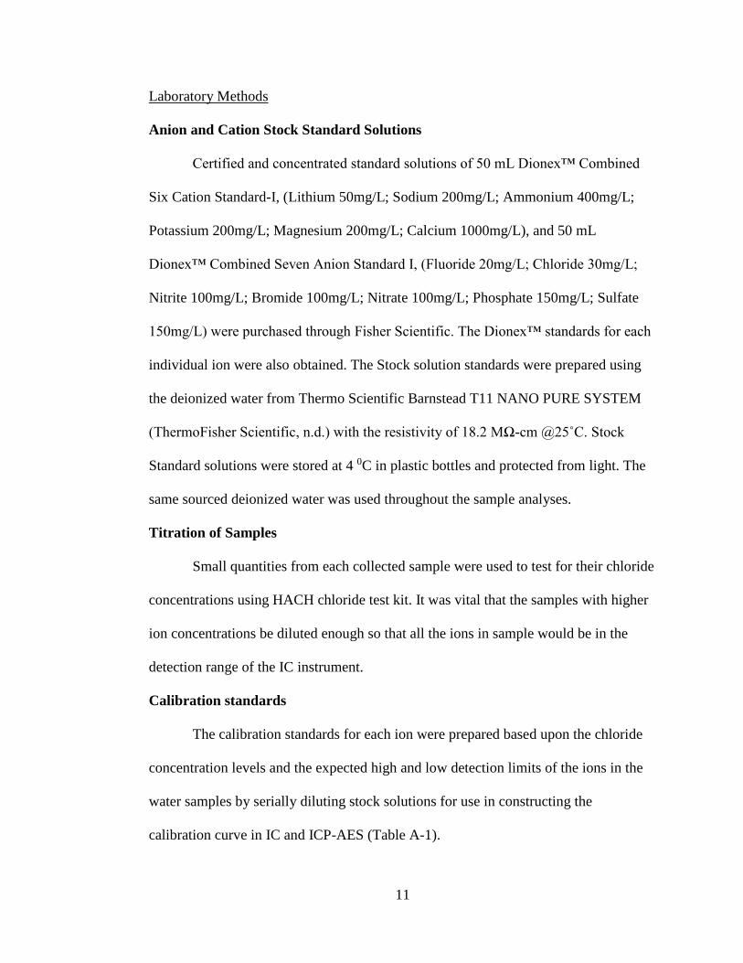
Laboratory Methods

Anion and Cation Stock Standard Solutions

Certified and concentrated standard solutions of 50 mL Dionex™ Combined

Six Cation Standard-I, (Lithium 50mg/L; Sodium 200mg/L; Ammonium 400mg/L;

Potassium 200mg/L; Magnesium 200mg/L; Calcium 1000mg/L), and 50 mL

Dionex™ Combined Seven Anion Standard I, (Fluoride 20mg/L; Chloride 30mg/L;

Nitrite 100mg/L; Bromide 100mg/L; Nitrate 100mg/L; Phosphate 150mg/L; Sulfate

150mg/L) were purchased through Fisher Scientific. The Dionex™ standards for each

individual ion were also obtained. The Stock solution standards were prepared using

the deionized water from Thermo Scientific Barnstead T11 NANO PURE SYSTEM

(ThermoFisher Scientific, n.d.) with the resistivity of 18.2 MΩ-cm @25˚C. Stock

Standard solutions were stored at 4 0C in plastic bottles and protected from light. The

same sourced deionized water was used throughout the sample analyses.

Titration of Samples

Small quantities from each collected sample were used to test for their chloride

concentrations using HACH chloride test kit. It was vital that the samples with higher

ion concentrations be diluted enough so that all the ions in sample would be in the

detection range of the IC instrument.

Calibration standards

The calibration standards for each ion were prepared based upon the chloride

concentration levels and the expected high and low detection limits of the ions in the

water samples by serially diluting stock solutions for use in constructing the

calibration curve in IC and ICP-AES (Table A-1).

12

Eluent Solution

The DX-500 IC requires the eluents 0.5 M sodium bicarbonate, 0.5M sodium

carbonate, and 05M sodium bicarbonate-sodium carbonate eluent.

Sample preparation

Samples were individually diluted based upon their titration results and their

expected ionic detection limits. For IC, samples were diluted as a solution of 1:10,

1:100, 1:1000, or no dilution was done. For ICP-AES, two sets were prepared. Set one

contained all the non-diluted samples. Set two was diluted as 1:10, prepared by taking

5mL of sample and adding 45 mL of 2% HNO3 to reach a final volume of 50mL in

falcon tubes. Samples were diluted as per the protocol in appendix (Table A-2) and

taken to the Brown University laboratory for anion and cation analysis. Samples were

allowed to equilibrate to room temperature before analysis.

Procedural Lab Blanks

a) Blank preparation for IC:

IC procedural blanks were prepared by taking two 60 mL syringes, filled with

deionized water. They were flushed three times, and then, for the fourth time, filled

while attached with a Millipore Sterivex syringe-filter (22µm pore size) and emptied

into 50 mL falcon tubes. Two falcon tubes were prepared for use as blanks.

b) Blank preparation for ICP-AES:

Two 60 mL syringes were each filled with 20 mL of 2% HNO3. Syringe were

covered at end with thumb and rotated to agitate the syringes so that both were all

agitated inside with the 2% HNO3. The 2% HNO3 was drained, and procedure was

13

repeated three times. The fourth time, syringes were filled with 50 mL of 2% HNO3.

Two of these were prepared for use as blanks.

Quality Controls

In addition to the standards prepared, the IC and ICP-AES used internal check

standards different from the calibration standards. For IC the FAS1, and for ICP-AES

QC28 were used, both available from Inorganic Vendors. FAS1 is a 5-anion standard

(Fluoride 0.2mg/L; Chloride 0.3mg/L; Nitrate 1mg/L; Phosphate 1.50mg/L; Sulfate

1.5mg/L), that is now sold as FAS 1A as a 7-anion standard (additional Bromide

1mg/L; and Nitrite 1mg/L).

The QC28 (Quality Control Standard 28) is a 125mL certified reference

material set in a nitric acid / hydrofluoric acid matrix for stability. It is a multi-analyte

custom made solution (Al, As, Be, Cr, Cd, Cu, Pb, Mg, Mo, K, Na, Tl, V, Sb, Ba, B,

Ca, Co, Fe, Li, Mn, Ni, Se, Ag, Sr, Ti, Zn as 1mg/L and Si as 0.5mg/L).

Instrumentation

Dionex Modular DX 500 Ion Chromatography system

The detection of anions (F-, Cl-, SO4-2, NO3

-) was done by measuring the

conductivity of the separated anions as they eluted from the separation column based

upon their affinity with the ion exchange column in the IC. The water samples were

analyzed for their anion makeup by the use of Dionex Modular DX 500 Ion

Chromatography system at the Brown University, Providence. The samples were

prepared as two sets. Set one was non-diluted but filtered for removal of chloride. The

samples were filtered for chlorine by running through the Fisher Scientific silver

cartridges. Set two was diluted as per the dilution protocol per each sample. The

14

anions present were identified by their retention times, and their quantities were

determined by the area of their peaks. The determination of peak parameters (area,

height, retention time) was done using Dionex software. The samples were from 9

wells: OCSW, CSW 1-1, CSW 1-2, CSW 1-3, CSW 1-4, CSW 1-5, QV 1-1, QV 1-2,

QV 1-3, and two were from a surface water creek site: TC1 and TC2.

Thermo Scientific iCAP 7400 Duo Inductively Coupled Plasma Atomic Emission

Spectrometer system

The well water samples were analyzed for their cation makeup (Ca+2, Na+, Mg+2,

K+) by the use of Thermo Scientific iCAP 7400 Duo Inductively Coupled Plasma

Atomic Emission Spectrometer system at the Brown University, Providence. An ICP-

AES system is made up of two parts: the inductively coupled plasma source, and the

atomic emission spectrometry detector. The principal behind the working of ICP AES

is the excitation of the samples as electrons, which emit energy at a diagnostic

wavelength as they return to their ground states. The emitted energy is characteristic

of each element and the intensity of energy is proportional to the concentration of that

element. This method identifies the elemental wavelength, and their intensities, the

ionic composition can be identified and quantified, relative to a standard. For ICP-

AES analysis, the samples were prepared as two sets: Set one was non-diluted. Set two

was diluted as 1:10. A total of 11 collected samples were tested for their cation

composition, namely Old Core Shed Well (OCSW), Core Shed Wells (CSW 1-1,

CSW 1-2, CSW 1-3, CSW 1-4, CSW 1-5), Quarry wells (QV 1-1, QV 1-2, QV 1-3),

Temptation Creek (TC1, TC2).

Data Analysis

15

Principal Components Analysis

JMP Statistical Data Analysis Software (JMP version 10) was used to explain

key factors and processes controlling the water chemistries at Coast Range Ophiolite.

Water chemistry data and related environmental parameters (with exception of depth)

were entered for multivariate statistical analysis and subjected to correlation matrix.

Eigenvalue Pareto Plot, Score Plot, and Loading Plot were generated to extract

information on the correlating factors.

Geochemist's Workbench

Geochemist's Workbench (GWB) REACT mode was used to model the low

temperature alteration of a serpentinization-influenced water package passing through

serpentinite host rock environment. React mode is a program in GWB that models and

simulates reactions taking takes in a geochemical system. The REACT mode can trace

the evolution of a system as it undergoes reactions in open and closed systems, under

various defined conditions.

The conceptual model of the REACT mode simulation is shown in Figure 4

(Bethke & Yeakel, 2015). An initial system is defined, and then the REACT program

calculates the system’s initial equilibrium state. The program then simulates a reaction

path by adding or removing reactants and adjusting the reaction conditions

accordingly. The results are generated as an output dataset and calculations are broken

down in a tabular form. REACT works by using the built-in rate laws for different

reactions (mineral dissolution and precipitation; aqueous and surface complex

dissociation and association; redox; microbially mediated reactions; gas transfers).

16

The inputs used in GWB modeling are shown in Table 1, Table 2 and Table 3.

Minerals including antigorite, magnetite, greenalite react with four types of input

waters (seawater, 10% dilution of seawater, local meteoric water, ultrabasic

groundwater). The system is water-dominated, simulating reactions taking place about

1 to 3 meters below land surface at CRO.

17

RESULTS

The water samples collected at CRO are from nine wells, contextualized by one

nearby groundwater-fed alkaline seep (Temptation Creek, TC), from which high

elevation (TC1) and low elevation (TC2) samples were obtained. The three Quarry

Valley wells (QV1-1, QV1-2, QV1-3) and six Core Shed wells (OCSW, CSW1-1,

CSW1-2, CSW1-3, CSW1-4, CSW1-5) sample from different depths in peridotite

bedrock at CRO (Figure 5) The QV wells are all within 3m of the main QV1-1 well,

from which rock cores were obtained. The CSW wells are within 5m of the main

CSW1-1 well, which also produced cores.

The key environmental parameters collected at CRO are shown in Table 4. The

environmental parameters noted on site were the pH, temperature (°C), conductivity

(EC, in mS/cm), dissolved oxygen (DO, in mg/L), and oxidation reduction potential

(ORP, in mV, corrected to Eh by addition of 200 mV to the value observed in the

field). The concentrations for major anions and cations are expressed as mg/L in Table

5.

The Ca/Mg ratios for TC1, TC2 and CSW1-4 are <1, dominated by Mg+2; while

the rest of the wells (OCSW, CSW1-1, CSW1-2, CSW1-3, CSW1-5, QV1-1, QV1-2,

QV1-3) are >1, dominated by Ca+2 (Figure 6).

The high Ca+2 and Mg+2 concentration values for all the CRO samples can be

seen in the Figure 7.

18

Another notable ionic composition of the CRO waters is their extremely high Na+

and Cl- concentrations (Figure 8). The Na+ and Cl- concentration overload is many

times higher than that of the seawater.

When the individual Na+ and Cl- concentration cross-plot is graphed for the CRO

samples and seawater, with the trendline passing through the SW, it can be seen that

the Na/Cl ratio is low for QV1-1, CSW1-5, OCSW and high for QV1-3, CSW1-1,

whereas the remaining wells QV1-2, CSW1-2, CSW1-3, CSW1-4 appear to be

dilutions of seawater as they remain very close on the seawater trendline (Figure 9). If

the increased Na drives these ratios up, there is possible Na desorption from clays or

albite dissolution, however if the low Na drives these ratios down, there may be

albitization of altered mafic (CSW site) or Na-sorption in the new smectite group

clays.

In Figure 9, the OCSW well, shows the most deviation in the Na+ and Cl- content

from the rest of the wells, being extremely high in Na+ as well as in Cl- concentrations

(Na+=1822ppm, Cl-=4041ppm).

Regarding the ratio of total Na+ ion content versus total Cl- ions, all the well

samples contain more Cl- ions than Na+ ions, which is the case for seawater’s Na+ and

Cl- content. An exception of this is present for the sole well CSW1-1 (Na+

=312.8ppm, Cl-=113.6 ppm). Here, Na+ concentration is higher than Cl-. The order of

wells from most to least is OCSW> CSW1-3> CSW1-5> CSW1-2> QV1-5> QV1-2>

QV1-3> CSW1-4> CSW1-1. The briniest OCSW is the deepest well (82m). The least

saline is CSW1-1 (the sole well with more Na+ than Cl-), and second-from-least-saline

CSW1-4 is the shallowest well (8.8m) in the entire set of monitoring wells. The

19

proximity of the CSW1-1 to CSW1-2 is also of interest as not only are the two wells

close to each other but are also of very similar depths (CSW1-1=19.5m, CSW1-

2=19.2m), yet where the CSW1-2 is the fourth most saline one (with similar Na+/Cl-

ratio to that of the seawater), but CSW1-1 is the least saline of all. Overall, the Core

Shed Valley wells are brinier than the Quarry Valley wells (with the exception of

CSW1-1, and least deep CSW1-4).

The in-field temperature measurements of the samples show the highest

temperature bearing well as the OCSW (17.810C), with the QV1-2 (17.350C) being

very close to the OCSW. Though the OCSW is the deepest and warmest in

temperature, the data for other wells and springs show no correlation between the

temperature and depth. Overall, the temperature range very close for the CSW and QV

wells (between 15-170C), and the temperatures for the TC1 and TC2 are on slightly

lower side of ~ 13-140C.

The deepest OCSW has the highest electrical conductivity (EC) of 11.44 mS/cm,

and the shallowest CSW1-4 has the least EC reading of only 1.86 mS/cm, though no

direct relation is seen for the EC and depth in the other wells (Figure 10). With the

exception of the OCSW (deepest) and CSW1-4 (shallowest), the CSW wells are

~5mS/cm in range, the QV wells are on slightly lower EC range of ~4mS/cm, and

TC1 and TC2 both show almost the same EC of ~3mS/cm.

The dissolved oxygen (DO) is highest for the shallowest well CSW1-4 (19.5%

DO), while its neighboring well CSW1-3 has the lowest DO of 0.7%. The range for

QV wells for DO is ~2-5%, and ~1-2% DO for CSW wells and the TC springs. There

20

is no apparent relationship of DO% with bottom of well depth; though the shallowest

well (CSW1-4) does reflect the greatest well DO reading of 19.5%.

The Eh values range from +418mV (TC1) to -110mV (CSW1-1). Using Garrels

and Christ (1965) plot that shows the Eh-pH relation of waters of various natural

environments, OCSW, CSW1-1, and CSW1-5 plot at pH of between 10-14, with very

negative Eh values, plotting within natural environments that are isolated from the

atmosphere. TC1 and TC2 plot around pH 8, with positive Eh values, signalling

environments in contact with the atmosphere (Figure 11).

The pH ranges for samples are from 13.5 to 7.6 in the following order: CSW1-1>

QV1-1> CSW1-3> OCSW> CSW1-5> QV1-3> QV1-2> CSW1-2> TC2> TC1. The

highest pH well CSW1-1 has the lowest Eh value, while the lowest pH site TC1 has

the highest Eh value; however, no linearity exists between the other samples.

The graphs for EC (as a proxy for total dissolved solids) and ionic concentrations

for CRO show similar curve profiles for both, except for CSW1-1 (Figure 12). The

unique ionic composition and concentrations that makes CSW1-1 differ from other

CRO wells, can further be seen in the Stiff diagrams of the samples created in the

GWB (Figure 13). The Stiff diagram for OCSW is most unique among the CRO

samples, followed only by CSW1-1. The CSW1-2, CSW1-4, and QV1-2, show similar

ionic compositions, though the concentrations seem to shift amongst the samples,

while maintaining the same overall Stiff diagram features. The Stiff diagrams for TC1

and TC2 are very closely related with each other, showing more ionic concentration of

the same makeup present in TC1, than for TC2.

21

Overall, the ionic concentrations of all the CRO samples, MW and SW show

that the CRO samples distinguish themselves from other waters due to their extremely

high Na+- Cl- concentrations, followed by the high Mg+2 and Ca+2 concentrations. The

complete concentration range of all the anions and cations can be seen in Figure 14.

The principal components analysis shows that the first two principal

components together account for 64.4% (41+23.4=64.4) of the total variation in the

data. The 1st component (PC1) accounts for 41% of the variation, and the 2nd

component (PC2) accounts for 23.4% of the variation in the data set (Figure 15).

The Loading Plot shows that if divided vertically into two equal halves, the

right half side shows factors that are positively correlated to the 1st component. These

factors include Ca+2, K+, NO3 -, Mg+2, and F-. The left half side includes factors that

are negatively correlated to the 1st component. These include DO, SO4-2, pH,

temperature, conductivity, Na+ and Cl-. The top right quadrant (I) containing Ca+2, K+,

NO3 -, Mg+2 show positive correlations with 2nd component (and are also positively

correlated with the 1st component). The lower right quadrant (IV) containing F- shows

the negative correlation with the 2nd and positive with the 1st component. The top left

quadrant (II) containing pH, temperature, conductivity, Na+ and Cl- show negative

correlation with 1st and positive correlation to the 2nd component. Similarly, the lower

left quadrant (III) containing DO and SO4-2 show negative correlation to 1st as well as

2nd component.

The scatter plot representation of the first two principal components can be

seen in the Score Plot. Here, the triangles represent the Temptation Creek, circles are

the Core Shed Wells, and the squares are the Quarry Valley Wells. Temptation Creek

22

data for both sites (TC1, TC2) lies in quadrant I, showing positive correlation with

first and second components in regards to Ca+2, Mg+2, K+, and NO3 -. The majority of

the clustering is within the quadrant III which shows the negative correlation of 1st and

2nd components in regards to their DO and SO4-2 content. The OCSW is plotted as

being the furthest from all the data points (quadrant II). Therefore, the OCSW shows a

marginal difference in Na+, Cl-, conductivity, temperature, and pH from all the rest of

the water samples. The correlations data table is provided in the (Table 6).

The GWB software was used to simulate the possible reaction pathways using

the input minerals from X-ray diffraction (XRD) profiles of the cores taken from CRO

(Cardace et al., 2013) with four types of water inputs (seawater, 10% dilute seawater,

local meteoric water, ultrabasic groundwater). The minerals were made to react at

three different temperatures (250C, 1000C, 20C). The GWB software predicted the

changes in pH, Eh, mineralogy, and in fluid chemistry as the serpentine-rich

environment reacted with the different waters over a total time span of 100 million

years (Ma). The software inputs are listed in Tables 1-3. It should be noted that for the

ultrabasic groundwater reacting with serpentine, the system could only proceed to

reach completion at the temperature of 250C. Under 1000C the residual was too large,

and at 20C the initial solution was too supersaturated to proceed.

Changes in pH at 250C:

In the case of the seawater reacting with serpentine, there is a small pH increase in the

initial 15 Ma (starting from time= 0 Ma), however the system gains a stable pH soon

and then stabilizes itself for the rest of the defined time period. In the case of the dilute

seawater a very small pH increase occurs in the very beginning, however the pH drops

23

back to the original very soon and stays close to the starting pH for the rest of the time

period. The model for meteoric water shows an impressive and sharp increase in pH

immediately after the system starts to react. The high pH increase is achieved very

quickly within the first few years and then the system stabilizes itself somewhat, with

a very gradual increase over the 100 Ma. The model for the ultrabasic groundwater

shows a high starting pH value that continuously keeps on decreasing with the passage

of time. Even after 100 Ma, the system still maintains high pH values with no

stabilization (Figure 16).

Changes in Eh at 250C:

The Eh models for seawater and dilute seawater show a steep and immediate decrease

in values (reaching very high negative values) followed by stabilization within the first

10-15 Ma. The meteoric seawater shows a similar immediate drop in Eh, however the

Eh drop reach extremely high negative values within the first 5 Ma. Starting from

zero, the Eh value drops to negative 340, followed by brief stabilization and then

dropping again to reach negative 400, and finally gaining somewhat stabilization for

the remaining time period. The last model that includes the ultrabasic groundwater

shows the most Eh variation over 100 Ma. It decreased to high negative values like the

other three models, but unlike the others, the system struggles to gain stabilization.

Even after 100 Ma, the system’s redox potential is still changing (Figure 17).

Changes in fluid chemistry at 250C:

In the case of the seawater, notable shifts are seen in Al+++, Fe++, H+, SiO2(aq) and

HCO3- ions for the first 20 Ma. Al+++, Fe++ increase, SiO2(aq) increase and then

decrease, and H+, and HCO3 decrease. For the dilute seawater, a slight concentration

24

increase takes place for Al+++, Fe++, SiO2 (aq) and H+. The system attains stability

within the first 10 Ma. The meteoric water shows different ionic fluctuations. Unlike

the first two models, Fe++ drops but then reaches back to the same initial concentration

within 20 Ma. H+ shows increase in concentration as in the dilute seawater scenario,

but with much steeper gradient and more quickly. Instead of Al+++, SO4-- shows a

notable decline during the first 20 Ma, after which the water chemistries show no

noticeable change. The ultrabasic groundwater shows the most evolved waters, that

are still changing after 100 Ma. The changes involve leaching of ions that include

Fe++, SiO2(aq) and HCO3- into the waters. The ions that decrease in the fluids are Al+++

and SO4--. Even after the 100 Ma, the waters are still reacting and evolving in this

mode (Figure 18).

Changes in mineralogy at 250C:

The models for seawater show emergence of a few different minerals during the first

20 Ma. The mineral makeup after 100 Ma includes dolomite (carbonate mineral),

saponite-Na (smectite group clay mineral), phlogopite (mica family of phyllosilicate),

hematite (oxide mineral), pyrite (sulfide mineral), muscovite (hydrated phyllosilicate),

phengite (mica group), quartz (oxide), Talc (silicate mineral) and the antigorite clays

minerals. The mineral that shows the most significant increase in concentration is

Hematite (within 10 Ma). Overall, antigorite is the most abundant mineral. The dilute

seawater shows simpler mineralogy consisting of saponite-Mg (smectite group clay

mineral), muscovite (hydrated phyllosilicate), hematite (oxide mineral), pyrite (sulfide

mineral), gibbsite (aluminum hydroxide), and phlogopite (mica family of

phyllosilicate), with emergence of Hematite after 10 Ma. The meteoric water shows

25

antigorite (most abundant), saponite-Mg, clinochl 14A (chlorite mineral), magnetite,

hematite, Ripidolite 14A (chlorite mineral), and pyrite. Magnetite appears after 20 Ma,

however Ripidolite 14A appears to be an indicator mineral as it appears after 80 Ma.

The ultrabasic model shows most dynamic mineralogy with emergence of various

minerals over the entire time period. Here, the notable minerals forming are magnetite

(after ~40 Ma), FeO (~60 Ma) with the most recent one being annite (~90 Ma). The

mineralogy at the end of 100 Ma includes presence of antigorite (most abundant),

phlogopite, andradite (garnet group mineral), wollastonite (inosilicate mineral),

clinochl 14A (chlorite group), diopside (inosilicate mineral), calcite (carbonate),

hematite, magnetite, FeO, annite (phyllosilicate mineral of mica family), and pyrite

(Figure 19).

pH variations among different temperature models:

The pH at 250C and 20C for seawater, dilute sea, and meteoric water (no ultrabasic

water model present) show very similar patterns. All three types of waters show an

initial increase in pH (dilute seawater pH drops down after the initial increase).

However, the pH model at 1000C show decreasing pH values for seawater and dilute

seawater. In the case of the meteoric water model at 1000C, it shows the same pH

increase as seen in meteoric waters at 250C and 20C temperatures (Figure 16, 20,21).

Eh variations among different temperature models:

Like the pH patterns, the Eh at 250C and 20C for seawater, dilute sea, and meteoric

water (no ultrabasic water model present) show very similar patterns. The seawater at

250C and 20C show same patterns of decrease in redox potential. The dilute seawaters

of 250C and 20C also show similar behavior to each other. Likewise, the meteoric

26

waters at 250C and 20C show patterns identical to each other. All four types of waters

at 250C and 20C, show trend of decreasing redox values, resulting in very reducing

waters. In the case of the model for 1000C, both the seawater and dilute seawater

decrease in Eh values like the waters at 250C and 20C, however instead of gaining

stability the values show increase before finally achieving stability. The behavior of

meteoric water for 1000C is the same as that of meteoric waters at 250C and 20C

(Figure 17, 22, 23).

Fluid chemistry variations among different temperature models:

Like pH and Eh, the seawaters and the meteoric waters at 250C and 20C show

similarities as the same ions undergo changes in similar ways, for both temperature

models. The dilute seawater models for 250C and 20C are also similar to each other.

However, at 1000C, the seawater shows a different water chemistry with HCO3- and

H+ leaching into the waters, and Al+++ with an initial increase and then stabilizing. The

meteoric water at 1000C also behaved differently than that of other temperature

models. SO4-- concentrations remain higher in this model, and unlike the absence of H+

under 250C and 20C, here H+ is produced after 70 Ma (Figure 18, 24, 25).

Mineralogy variations among different temperature models:

The greatest variation due to temperature difference is present in the mineralogy of the

models. The input minerals included antigorite, beidellite-Mg, brucite, clinochi-7A,

greenalite, and magnetite. The seawater end products include antigorite, saponite-Na,

dolomite, phlogopite, hematite, pyrite, muscovite, phengite, nontronite-Na, talc and

quartz. No new minerals are forming beyond the first 15 Ma. In the case of 1000C the

mineralogy includes antigorite, dolomite, hematite, pyrite, brucite, saponite-Mg, and

27

clinochl 14A. New minerals are forming after 15 Ma. In the case of 20C, the end

minerals are antigorite, saponite-Mg, clinochl 14A, hematite, pyrite, talc, saponite-Ca,

with the emergence of Ripidolite 14A around 25 Ma. In the case of dilute seawater,

250C shows very simple mineralogy makeup consisting of saponite-Mg, hematite,

pyrite, muscovite, phlogopite, and gibbsite. No antigorite is present. At the

temperature of 1000C, we see appearance of different minerals over time. It includes

all the minerals of 250C (except phlogopite) and also additional ones that include

amesite 14A, clinochl 14A, dolomite, and antigorite. The emergence of muscovite

and gibbsite takes place after 40 Ma. At 20C, the mineralogy is simple like in 250C

model, with the minerals saponite-Na, hematite, pyrite, muscovite, dolomite, and a

different mineral nontronite-Na emerging after ~60 Ma. In the case of meteoric

waters, all three temperature models include antigorite, saponite-Mg, clinochl 14A,

magnetite, hematite, and pyrite. What sets these apart is the formation of Ripidolite

14A after 80 Ma (at 250C), absence of Ripidolite 14A (at 1000C), and presence of talc

and saponite-Ca (at 20C) (Figure 19, 26, 27).

28

DISCUSSION

The process of serpentinization leads to the formation of waters that are

extremely rare in the natural environments (Neal, 1984; Chavagnac et al., 2013). The

physical and chemical data from CRO shows the presence of Type I and Type II

waters at CRO. The Ca/Mg ratios show that TC1, TC2 and CSW1-4 are Type I (high

Mg+2) open system waters. OCSW, CSW1-1, CSW1-3, and QV1-1 are the Type II

(high Ca+2) closed system water. CSW1-2, CSW1-5, QV1-2, and QV1-3 are found to

be the intermediate, mixed water (Figure 28). CSW1-4, the shallowest of all the wells,

is an open water system, unlike any other groundwater wells. High pH, high Ca+2-OH-

waters, and lower pH, high Mg+2-HCO3- waters are unique to serpentinizing sites

(Barnes and O’Neil, 1969; Paukert et al., 2012).

All the samples show high Na+ and Cl- concentrations. This is due to the reaction

of Cretaceous seawater trapped within the ophiolite during its emplacement and

reacting with the surrounding rocks (Peter, 1993; Schulte, 2006). The stable isotope

data from CRO also supports presence of seawater as the serpentinizing fluid (Barnes

et al., 2013). The OCSW shows the greatest Na+ and Cl- concentration due to being

the deepest with more surface area for interacting with altered fluids and bedrock

constituents. CSW1-2, CSW1-3, CSW1-4, and QV1-2 show similar Na+ and Cl- ratios

as that of sea water, therefore they appear to be dilutions of varying extent of the

trapped sea waters. These dilutions of SW can be due to the influx of meteoric and

other shallowly sourced waters.

29

All the well samples maintain the same Cl- > Na+ content as in seawater, with the

exception of CSW1-1. CSW wells are brinier than the QV wells. Despite the close

proximity of all the CSW wells to each other, CSW 1-1 is least saline of all the wells,

including the QV wells. One of the possible explanation that puts CSW1-1 apart from

others might be a result of casing. All the wells except for CSW1-1 and QV1-1 were

cased with PVC pipes. The CSW1-1 and QV1-1 are also larger in diameter than the

other pipes (Twing et al., 2017).

Temperature profile of the wells show variations that are irrespective of the depth.

The subtle temperature variations noted here are seasonal and site-specific (related to

heat from solar radiation striking the land surface, conducted to some depth below the

land surface), or in-flow of regional geothermal waters. Using Garrels and Christ’s

Eh-pH plot for finding the limits of the naturally occurring aqueous environments,

OCSW, CSW1-1, and CSW1-5 show stability range within environments that are

isolated from the atmosphere (Figure 29). These are the highly alkaline waters with

strong reducing values. The two alkaline springs (TC1, TC2) are in the environment

that are in contact with the atmosphere and thereby have the most oxidizing values,

while still being slightly alkaline. The rest of the samples, CSW1-2, CSW1-3, CSW1-

4, QV1-2, QV1-2, and QV1-3 show properties of transitional environments, and are in

the spectrum of high alkaline waters. Overall, CSW groundwaters are more reducing

than the QV ones. Based upon this data, a graphical representation showing observed

bedrock-water interactions for the wells and spring waters, is proposed in Figure 30.

GWB software was used to predict the changes that took place over the 100 Ma

time frame, using four kinds of input waters (seawater, 10% dilute seawater, meteoric

30

water, ultrabasic groundwater) and under three different temperature settings (2OC,

25OC, 100OC). The GWB software showed no effect of temperature for 2OC and

25OC. In both models, the pH increases sharply for meteoric water, gradually for

seawater, and a very small change in the case of dilute seawater. This is consistent

with the observed high alkaline pH values for CRO as well as other known

serpentinizing site. Similarly, the results for Eh showed no effect of temperature over

Eh changes. All kinds of water, at all three temperatures, showed the decreasing (high

negative) Eh values which are consistent with extremely reducing waters as observed

in field at CRO and other serpentinizing sites. The software also showed leaching of

minerals in and out of the water as it flows through the bedrock, with corresponding

mineralogical changes in the serpentine rich environment. Leaching of the ultramafic

rocks into the reacting waters is considered to be influenced by the chemical properties

of water, the temperature, pressure, and the chloride content (Moody, 1976). The

models for all the waters show that the leaching is lowest for 2OC, with an increase for

25OC, and the most leaching taking place at 100OC. Study on Oman and Ligurian

ophiolites show that the fluid compositions vary among one ophiolite to another, and

also within the same ophiolite (Chavagnac et al., 2013).

The main ions that take place in noticeable chemical changes in waters are Al+++,

Fe++, H+, SiO2(aq), SO4--

and HCO3-. Major changes are noted for the first 20 Ma,

however the model for the ultrabasic groundwater show considerable changes

throughout the 100 Ma. Generally, the concentrations of Al+++, SiO2(aq), and Fe++

show leaching in as well as out of the waters over time. These ions provide

explanation for corresponding mineralogical changes. The models for all three

31

temperatures show weathering of various minerals into their constituents, as well as

appearance of characteristic new minerals over time. Model show antigorite as the

most abundant serpentine mineral, which is a prograde metamorphism indicator

(Moody, 1976). Numerous smectites, phyllosilicates, inosilicates are formed. Al+++

concentrations in fluids are explained by the emergence of albites (saponite-Na,

muscovite, annite, gibbsite). This also provides the answer to the observed Na/Cl

ratios in the CRO groundwaters (Figure 9). GWB modeling suggests that it must be

the low Na that drove the Na/Cl ratio down due to albitization of altered mafic and/or

Na-sorption in the new smectite group clays. Changes in observed Fe++ concentration

in fluid waters can be the result of formation of hematite, pyrite, and magnetite. Annite

(ultrabasic model at 25OC) appears to one of the marker minerals forming during the

last 15 Ma (around ~85 Ma and onwards). Also, a smectite nontronite is formed in

dilute seawater at 2OC (as an apparent marker mineral, appearing ~60 Ma after start of

serpentinization process) and seawater at 25OC. Nontronite (dioctahedral smectite) has

been found on Mars surface by orbiting CRISM (Compact Reconnaissance Imaging

Spectrometer for Mars) (Morris et al., 2010) and OMEGA (Observatoire pour la

Mine´ralogie, l’Eau, les Glaces, et l’Activite) (Bibring, et al., 2005). Along with the

smectite clay minerals, kaolinites have also been found at Mars (Baumeister et al.,

2011). All the GWB models show the formation of antigorite, hematite, muscovite,

pyrite, and saponite. The ultrabasic groundwater model (25OC) show these same

minerals along with emergence of some minerals unique to this system only. These

include andradite, wollastonite, diopside, calcite, annite, and FeO(c). Andradite,

wollastonite, diopside, and calcite contain Ca++. Their presence only in the ultrabasic

32

model supports the presence of Ca++ in high alkaline, closed water systems (Type II).

Also, FeO(c) formation is limited to highly reducing environment (highly alkaline,

Type II). This is supported by the findings that Mg is completely depleted in waters of

pH 10.5 and higher, whereas Ca++ accumulates with pH increase (Chavagnac, 2013).

Among all the GWB models, the most difficult model to predict fluid

composition accuracy would be in the case of meteoric model because meteoric waters

undergo unpredictable compositional changes during runoff.

33

CONCLUSION AND FUTURE WORK SUGGESTIONS

The Coast Range Ophiolite can be considered a site of ongoing low

temperature serpentinization, with weathering related processes at work evidenced by

environmental and geochemical parameters (redox measurements, temperature, pH,

electrical conductivity, ionic composition). Physical parameters highlight that these

high pH and low Eh groundwaters fall into known ranges for serpentinizing systems.

The analytical chemistry confirms presence of different fluids that are reflective of

rock-water interactions. Ca+2-OH- and Mg+2-HCO3- waters are present and still

evolving. Use of the Geochemist’s Workbench provides insight into the changing fluid

chemistry and corresponding mineralogical changes in the bedrock. The software

further identifies the weathering profiles and appearance of indicator minerals (e.g.,

smectites, albites, chlorites) that not only reflect the weathered stage of post-

serpentinization, but also help in identification of serpentinizing terranes on Mars and

other serpentinization-related celestial bodies (e.g., Europa, Enceladus) in our Solar

System and beyond.

Future works are suggested in collection of soil samples from Coast Range

ophiolite and tested for modeling accuracy. The software Geochemist’s Workbench

did not allow for biological inputs, which are also an important aspect to consider in

water-rock reactions. Furthermore, the local rain samples’ isotope data can provide us

with more detailed insight into the complex weathering of serpentinites.

34

REFERENCES

Alexander, E. B., Coleman, R. G., Harrison, S. P., & Keeler-Wolfe, T. (2007).

Serpentine geoecology of western North America: geology, soils, and

vegetation. OUP USA.

Allen, D. E., & Seyfried Jr, W. E. (2004). Serpentinization and heat generation:

constraints from Lost City and Rainbow hydrothermal systems1. Geochimica

et Cosmochimica Acta, 68(6), 1347-1354.

Alt, J. C., Schwarzenbach, E. M., Früh-Green, G. L., Shanks III, W. C., Bernasconi, S.

M., Garrido, C. J., & Marchesi, C., (2013). The role of serpentinites in cycling

of carbon and sulfur: seafloor serpentinization and subduction

metamorphism. Lithos, 178, 40-54.

Andreani, M., Luquot, L., Gouze, P., Godard, M., Hoise, E., & Gibert, B. (2009).

Experimental study of carbon sequestration reactions controlled by the

percolation of CO2-rich brine through peridotites. Environmental Science &

Technology, 43(4), 1226-1231.

Barnes, I., & O'Neil, J. R. (1969). The relationship between fluids in some fresh

alpine-type ultramafics and possible modern serpentinization, western United

States. Geological Society of America Bulletin, 80(10), 1947-1960.

Barnes, I., LaMarche, V. C., & Himmelberg, G. (1967). Geochemical evidence of

present-day serpentinization. Science, 156(3776), 830-832.

Barnes, I., O'Neil, J. R., & Trescases, J. J. (1977). Present day serpentinization in New

Caledonia, Oman and Yugoslavia. Geochimica et Cosmochimica Acta, 42(1),

144-145.

Barnes, I., Rapp, J. B., O'Neil, J. R., Sheppard, R. A., & Gude, A. J. (1972).

Metamorphic assemblages and the direction of flow of metamorphic fluids in

four instances of serpentinization. Contributions to Mineralogy and

Petrology, 35(3), 263-276.

Barnes, J. D., Eldam, R., Lee, C. T. A., Errico, J. C., Loewy, S., & Cisneros, M.

(2013). Petrogenesis of serpentinites from the Franciscan Complex, western

California, USA. Lithos, 178, 143-157.

Berner, E. K., & Berner, R. A. (1987). Global water cycle: geochemistry and

environment. Prentice-Hall.

Bethke, C. M., & Yeakel, S. (2015). The Geochemist’s Workbench (Version 10.0):

Reaction modeling guide. Aqueous Solutions, LLC, Champaign, Ill.

35

Bibring, J. P., Langevin, Y., Gendrin, A., Gondet, B., Poulet, F., Berthé, M., ... &

Drossart, P. (2005). Mars surface diversity as revealed by the OMEGA/Mars

Express observations. Science.

Blank, J. G., Green, S. J., Blake, D., Valley, J. W., Kita, N. T., Treiman, A., &

Dobson, P. F. (2009). An alkaline spring system within the Del Puerto

Ophiolite (California, USA): a Mars analog site. Planetary and Space Science,

57(5), 533-540.

Burns, S. J., & Matter, A. (1995). Geochemistry of carbonate cements in surficial

alluvial conglomerates and their paleoclimatic implications, Sultanate of

Oman. Journal of Sedimentary Research, 65(1).

Cardace, D., Hoehler, T., McCollom, T., Schrenk, M., Carnevale, D., Kubo, M., and

Twing, K. 2013. Establishment of the Coast Range ophiolite microbial

observatory (CROMO): drilling objectives and preliminary outcome. Scientific

Drilling, 16: 45–55, www.sci-dril.net/16/45/2013/ doi:10.5194/sd-16-45-2013.

Cardace, D., Hoehler, T. M., McCollom, T. M., Schrenk, M. O., & Kubo, M. D.

(2014). Integration of 3 Consecutive Years of Aqueous Geochemistry

Monitoring Serpentinization at the Coast Range Ophiolite Microbial

Observatory (CROMO), Northern California, USA. In AGU Fall Meeting

Abstracts (Vol. 1, p. 4835).

Chavagnac, V., Monnin, C., Ceuleneer, G., Boulart, C., & Hoareau, G. (2013).

Characterization of hyperalkaline fluids produced by low‐temperature

serpentinization of mantle peridotites in the Oman and Ligurian ophiolites.

Geochemistry, Geophysics, Geosystems, 14(7), 2496-2522.

Chizmeshya, A. V., McKelvy, M. J., Squires, K., Carpenter, R. W., & Bearat, H.

(2007). A novel approach to mineral carbonation: Enhancing carbonation

while avoiding mineral pretreatment process cost. Arizona State University.

Choi, S. H., Shervais, J. W., & Mukasa, S. B. (2008). Supra-subduction and abyssal

mantle peridotites of the Coast Range Ophiolite, California. Contributions to

Mineralogy and Petrology, 156(5), 551

Corliss, J. B., Baross, J. A., & Hoffman, S. E. (1981). A hypothesis concerning the

relationships between submarine hot springs and the origin of life on earth.

Oceanologica Acta, Special issue.

D’Amico, M. E., & Previtali, F. (2012). Edaphic influences of ophiolitic substrates on

vegetation in the Western Italian Alps. Plant and soil, 351(1-2), 73-95.

Dickinson, W. R., Hopson, C. A., Saleeby, J. B., Schweickert, R. A., Ingersoll, R. V.,

36

Pessagno Jr, E. A., & Munoz, I. M. (1996). Alternate origins of the Coast

Range ophiolite (California): Introduction and implications. GSA today, 6(2),

1-10.

Ehlmann, B. L., Mustard, J. F., & Murchie, S. L. (2010). Geologic setting of

serpentine deposits on Mars. Geophysical research letters, 37(6).

Etiope, G. (2017). Abiotic methane in continental serpentinization sites: an

overview. Procedia Earth and Planetary Science, 17, 9-12.

Garrels, R. M., and Christ, C. L., 1965, Solutions, minerals, and equilibria: San

Francisco, California, Freeman, Cooper & Company, 450 p.

Geotech Environmental Equipment, Inc. (2018). Geotech Bladder Pumps: Installation

and Operation Manual. Retrieved January 10, 2017, from

http://www.geotechenv.com/Manuals/Geotech_Bladder_Pumps.pdf

Hill, S. J. (Ed.). (2008). Inductively coupled plasma spectrometry and its

applications (Vol. 8). John Wiley & Sons.

Kelemen, P. B., Matter, J., Streit, E. E., Rudge, J. F., Curry, W. B., & Blusztajn, J.

(2011). Rates and mechanisms of mineral carbonation in peridotite: natural

processes and recipes for enhanced, in situ CO2 capture and storage. Annual

Review of Earth and Planetary Sciences, 39, 545-576.

Lang, S. Q., Butterfield, D. A., Schulte, M., Kelley, D. S., & Lilley, M. D. (2010).

Elevated concentrations of formate, acetate and dissolved organic carbon

found at the Lost City hydrothermal field. Geochimica et Cosmochimica Acta,

74(3), 941-952.

Martin, W., Baross, J., Kelley, D., & Russell, M. J. (2008). Hydrothermal vents and

the origin of life. Nature Reviews Microbiology, 6(11), 805.

Mathany, T.M., and Belitz, K. (2015). Groundwater quality in the Northern Coast

Ranges Groundwater Basins, California: U.S. Geological Survey Fact Sheet

2014–3114, 4 p., https://dx.doi.org/10.3133/fs20143114.

Moody, J. B. (1976). Serpentinization: a review. Lithos, 9(2), 125-138.

Morris, R. V., Ming, D. W., Golden, D. C., Graff, T. G., & Achilles, C. N. (2010,

March). Evidence for interlayer collapse of nontronite on Mars from laboratory

visible and near-IR reflectance spectra. In Lunar and Planetary Science

Conference (Vol. 41, p. 2156).

Natural Reserve System University of California (2018). McLaughlin Natural

37

Reserve. Retrieved January 12, 2017, from

https://ucnrs.org/reserves/mclaughlin-natural-reserve/

Neal, C., & Stanger, G. (1983). Hydrogen generation from mantle source rocks in

Oman. Earth and Planetary Science Letters, 66, 315-320.

Neal, C., & Stanger, G. (1984). Calcium and magnesium hydroxide precipitation from

alkaline groundwaters in Oman, and their significance to the process of

serpentinization. Mineralogical Magazine, 48(347), 237-241.

Paukert, A. N., Matter, J. M., Kelemen, P. B., Shock, E. L., & Havig, J. R. (2012).

Reaction path modeling of enhanced in situ CO 2 mineralization for carbon

sequestration in the peridotite of the Samail Ophiolite, Sultanate of Oman.

Chemical geology, 330, 86-100.

Peters, E. K. (1993). D-18O enriched waters of the Coast Range Mountains, northern

California: Connate and ore-forming fluids. Geochimica et Cosmochimica

Acta, 57(5), 1093-1104.

Russell, M. J. (2007). The alkaline solution to the emergence of life: energy, entropy

and early evolution. Acta biotheoretica, 55(2), 133-179.

Safford, H. D., Viers, J. H., & Harrison, S. P. (2005). Serpentine endemism in the

California flora: a database of serpentine affinity. Madroño, 52(4), 222-257.

Salhi, E., & Von Gunten, U. (1999). Simultaneous determination of bromide,

bromate and nitrite in low μg l− 1 levels by ion chromatography without sample pretreatment. Water Research, 33(15), 3239-3244.

Schulte, M., Blake, D., Hoehler, T., & McCollum, T. H. O. M. A. S. (2006).

Serpentinization and its implications for life on the early Earth and

Mars. Astrobiology, 6(2), 364-376.

Szponar, N., Brazelton, W. J., Schrenk, M. O., Bower, D. M., Steele, A., & Morrill, P.

L. (2013). Geochemistry of a continental site of serpentinization, the

Tablelands Ophiolite, Gros Morne National Park: a Mars analogue. Icarus,

224(2), 286-296.

ThermoFisher Scientific. (n.d.). Thermo Scientific™ Barnstead™ Nanopure™

Accessories and Consumables. Retrieved August 13, 2017, from

https://www.thermofisher.com/order/catalog/product/D50280.

Tu, V., Baumeister, J., Metcalf, R., Olsen, A., & Hausrath, E. (2011). Serpentinite

weathering and implications for Mars.

Twing, K. I., Brazelton, W. J., Kubo, M. D., Hyer, A. J., Cardace, D., Hoehler, T. M.,

38

... & Schrenk, M. O. (2017). Serpentinization-influenced groundwater harbors

extremely low diversity microbial communities adapted to high pH. Frontiers

in microbiology, 8, 308.

University of California, Davis. (2003). Natural history of the McLaughlin Reserve:

Napa, Lake and Yolo counties California. Davis, Calif: University of

California, Natural Reserve System. Retrieved September 22, 2017, from

https://naturalreserves.ucdavis.edu/sites/g/files/dgvnsk1091/files/inline-

files/MCL_geology.pdf

Wildman, W. E., Jackson, M. L., & Whittig, L. D. (1968). Iron-Rich Montmorillonite

Formation in Soils Derived from Serpentinite 1. Soil Science Society of

America Journal, 32(6), 787-794.

39

FIGURES AND TABLES

Figure 1. Geologic map of the Coast Range, with the ophiolite exposures in solid

black, and the star indicating the location of McLaughlin Natural Reserve in Western

California (modified from Choi et al., 2008).

40

Figure 2. Global distribution of ophiolites, except Spain, Japan (peridotite massifs)

and Portugal (peridotite intrusion). Modified from Etiope, G. (2017).

41

Figure 3. Aerial map of the three main sampling locations from McLaughlin Reserve

created in Google Earth. The Quarry Valley Wells are named for historic quarrying of

shale beds in the vicinity. The Core Shed Wells are named for the nearby regional core

archive structure. A seasonally active groundwater-fed Temptation Creek is the third

area for sample collection, with its two sampling points and their elevation profile

shown inside the upper right box.

42

Figure 4. The conceptual model of the REACT mode simulation (Bethke & Yeakel,

2015).

43

Figure 5. Depth profile of the wells at McLaughlin Natural Reserve, California. The

QV wells are all within 3 m of the main QV1-1 well, from which rock cores were

obtained. The CSW wells are within 5 m of the main CSW1-1 well, which also

produced cores. The deepest well OCSW is 82 m deep.

44

Figure 6. Calcium to magnesium ratios, plotted on Y-axis, with the

sampling sites on X-axis. Ca/Mg ratios for TC1, TC2 and CSW1-4 are <1,

being dominated by Mg+2; while the rest of the wells (OCSW, CSW1-1,

CSW1-2, CSW1-3, CSW1-5, QV1-1, QV1-2, QV1-3) are >1, dominated by

Ca+2.

45

Figure 7. Ca+2 and Mg+2 ionic concentrations of CRO samples.

46

Figure 8. Sodium and Chloride ion composition present in the CRO samples.

47

Figure 9. XY plot of sodium and chloride ion concentration with sodium ions plot on

Y-axis, and chloride ions, on the X-axis. The trend-line passing through the seawater.

Upper right box: Enlarged view of the samples shown along SW trendline.

48

Figure 10. The electrical conductivity measured in mS/cm (milli second) and

expressed here in uS/cm (micro second) for graphing the CRO samples.

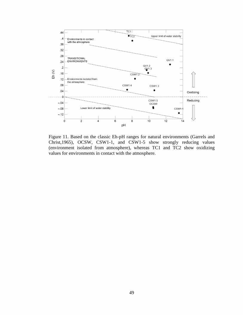
49

Figure 11. Based on the classic Eh-pH ranges for natural environments (Garrels and

Christ,1965), OCSW, CSW1-1, and CSW1-5 show strongly reducing values

(environment isolated from atmosphere), whereas TC1 and TC2 show oxidizing

values for environments in contact with the atmosphere.

50

Figure 12. The graph profiles for the electrical conductivity (as a proxy for total

dissolved solids) on the left, and the graph for the ionic concentrations of samples, on

the right. Both graphs show similar graph profile curves, with the exception of CSW1-1.

51

Figure 13. Stiff diagrams made in GWB showing the major ionic makeup and the

compositional variations/similarities as a visual graphic for CRO samples.

52

Figure 14. Ionic makeup of the 2017 CRO waters and. Overall, the ionic

concentrations of all the CRO samples show that the Coast Range fluid samples

distinguish themselves from other waters due to their high Na+- Cl- concentrations,

followed by the high Mg+2 and Ca+2 concentrations.

53

Figure 15: Principal components analysis results with Eigenvalue Pareto Plot (on the

left), Score Plot (in the middle), and Loading Plot (on the right). In the Score Plot, the

triangles (black and dark gray) represent Temptation Creek TC1 and TC2, circles

(light gray, yellow, orange, pink, light blue, light green) as Core Shed Wells, and

squares (red, dark blue, dark green) as Quarry Valley Wells.

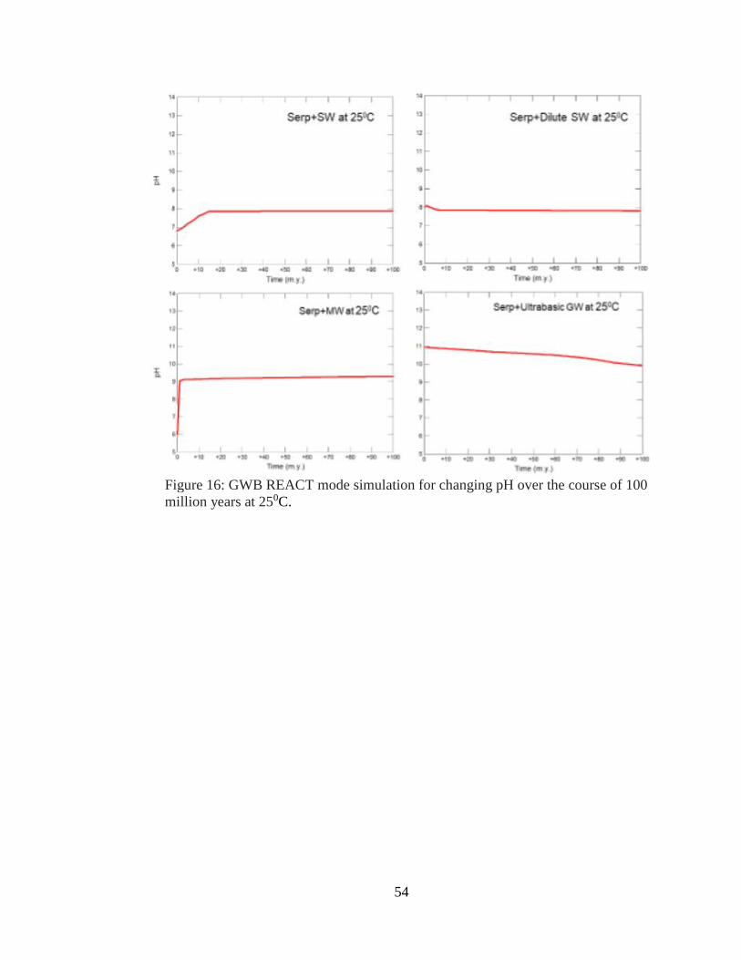
54

Figure 16: GWB REACT mode simulation for changing pH over the course of 100

million years at 250C.

55

Figure 17: GWB REACT mode simulation for changing Eh (mV) over the course of

100 million years at 250C.

56

Figure 18: GWB REACT mode simulation for changing fluid composition (mg/kg)

over the course of 100 million years at 250C.

57

Figure 19: GWB REACT mode simulation for changing mineralogy (volume%) over

the course of 100 million years at 250C.

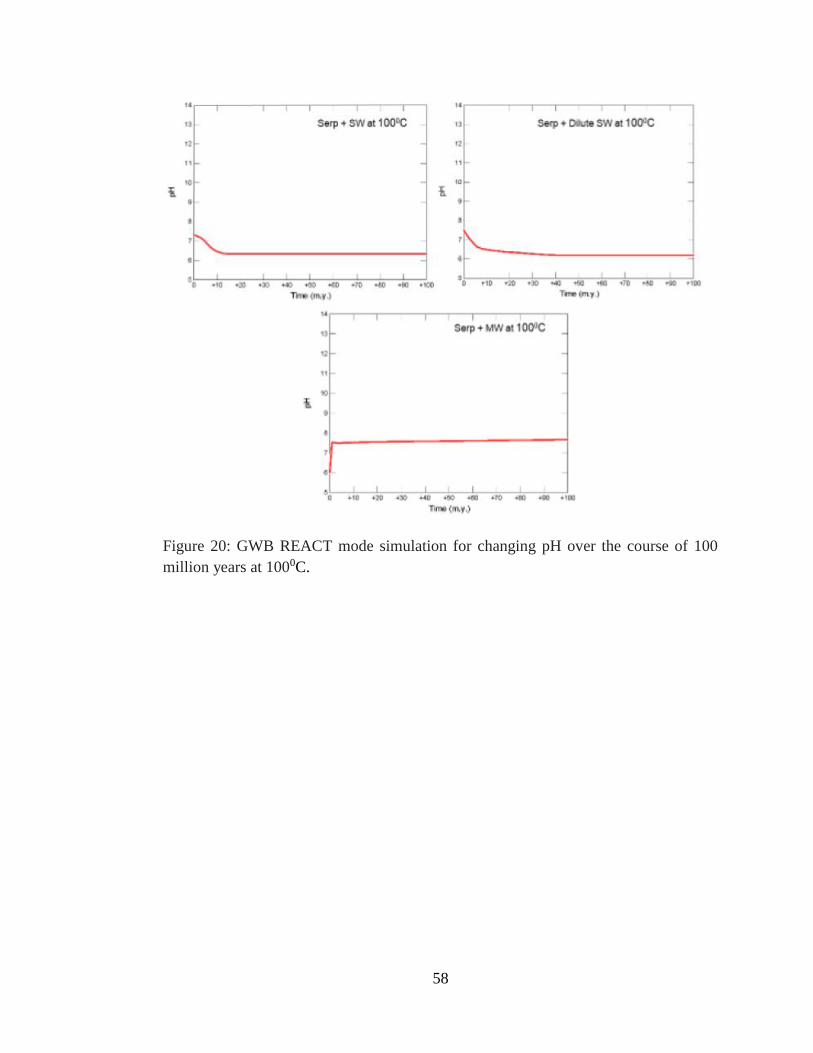
58

Figure 20: GWB REACT mode simulation for changing pH over the course of 100

million years at 1000C.

59

Figure 21: GWB REACT mode simulation for changing pH over the course of 100

million years at 20C.

60

Figure 22: GWB REACT mode simulation for changing Eh (mV) over the course of

100 million years at 1000C.

61

Figure 23: GWB REACT mode simulation for changing Eh (mV) over the course of

100 million years at 20C.

62

Figure 24: GWB REACT mode simulation for changing fluid chemistries (mg/kg)

over the course of 100 million years at 1000C.

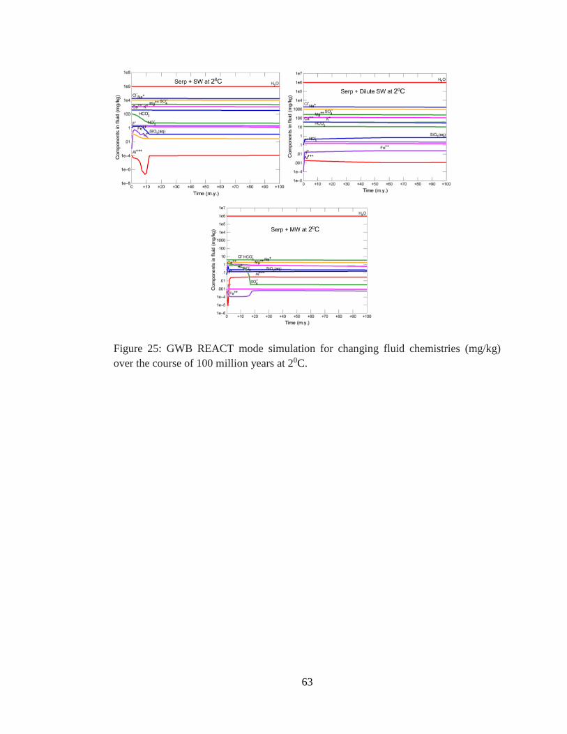
63

Figure 25: GWB REACT mode simulation for changing fluid chemistries (mg/kg)

over the course of 100 million years at 20C.

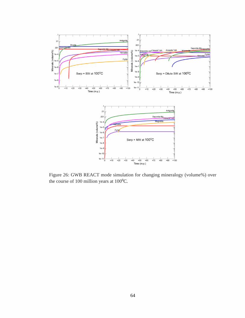
64

Figure 26: GWB REACT mode simulation for changing mineralogy (volume%) over

the course of 100 million years at 1000C.

65

Figure 27: GWB REACT mode simulation for changing mineralogy (volume%) over

the course of 100 million years at 20C.

66

Figure 28: Type I, Type II and the mixed waters, based upon the Ca/Mg ratios. TC1,

TC2 and CSW1-4 are Type I, open system waters. OCSW, CSW1-1, CSW1-5, and

QV1-1 are the Type II, closed system waters. CSW1-2, CSW1-5, QV1-2, and QV1-3

are the mixed waters.

67

Figure 29. Eh-pH plot (modified from Garrels and Christ plot for limits of the natural

environments, show OCSW, CSW1-1, and CSW1-5 as being strongly reducing. The

wells CSW1-4, CSW1-3, CSW1-2, QV1-3, and QV1-2 show decreasing reducing

trend with QV1-1 as the least reducing well. TC1 and TC2 are oxidizing waters.

68

Figure 30. Summary of bedrock-water interactions taking place at the Coast Range

ophiolite, as a framework for grouping CRO waters.

69

Table 1: The inputs used in GWB modeling. Geochemist's Workbench (GWB)

REACT mode was used to model the low temperature alteration of a serpentinization-

influenced water package passing through serpentinite rich environment. Three types

of input waters were used: meteoric water, seawater, and a 10% seawater solution.

Parameters Descriptions

Antigorite 0.5 mol/kg

Beidellite-Mg 0.1 mol/kg

Brucite 0.05 mol/kg

Clinochl-7A 0.1 mol/kg

Greenalite 0.2 mol/kg

Magnetite 0.05 mol/kg

Total mass input of solids 1 mol/Kg

Temperature 250C

Porosity 0.1

Water 1 kg free water + 0.1 kg/year

Initial pH 8

Time Frame 100 my

Pressure 1.0 bar

Type of water-rock system Water dominated

70

Table 2: Ionic composition of regional precipitation (MW) at Menlo Park, California,

from 1957-1959 (from Berner & Berner, 1987).

Ionic composition of regional precipitation at Menlo Park, California (1957-1959)

Ion Concentration (in mg/l)

Na+ 2.0

K+ 0.25

Mg++ 0.37

Ca++ 0.79

Cl- 3.43

SO4-- 1.39

NO3- 0.16

NH4+ _

Ca-/Na+ 1.7

pH 6.0

71

Table 3: Ionic composition of seawater (SW) (from Berner & Berner, 1987).

Major Dissolved Components of Seawater for a Salinity of 35% (*P=1 atm, T=250 C)

Ion Concentration in g/Kg

Na+ 10.77

K+ 0.399

Mg++ 1.290

Cl- 19.354

SO4-- 2.712

Ca++ 0.412

HCO3- * 0.12

72

Table 4: Field data collected in 2017. The environmental parameters noted on site

were the pH, temperature (°C), conductivity (EC, in mS/cm), dissolved oxygen (DO,

in mg/L), and oxidation reduction potential (ORP, in mV, corrected to Eh by addition

of 200 mV to the value observed in the field). TC1 and TC2 data here is from

December of 2012.

2017

Sample

ID

Temp

(°C)

Cond.

(mS/cm)

DO (%) ORP

(Eh,

mV)

pH Depth

(m)

OCSW 17.81 11.44 1.9 -76.6 10.52 82

CSW1-1 15.89 3.758 1.1 -110 13.54 19.5

CSW1-2 15.85 4.602 0.9 124.8 8.35 19.2

CSW1-3 15.69 4.794 0.7 45.2 10.64 23.2

CSW1-4 15.34 1.86 19.5 49.6 7.42 8.8

CSW1-5 15.89 4.905 0.9 -69.2 10.5 27.4

QV1-1 15.55 3.526 2 222.1 12.49 23

QV1-2 17.35 3.073 3.6 183.7 9.73 14.9

QV1-3 15.93 3.918 4.8 163.9 9.9 34.6

TC1 14.24 2.833 1.32 7.61

TC2 13.3 2.963 8.03

73

Table 5. Ionic Composition of the CROMO samples from 2017 (expressed in mg/L)

Ionic Composition of the CROMO samples from 2017 (expressed in

mg/L)

2017

Sample

ID

F- NO3- SO4-2

Cl-

K+ Na+ Mg+2 Ca+2

OCSW 0.018 9.437 4041 24.33 1822 0.06 76.13

CSW1-

1

0.22 0.262 40.444 113.62 31.28 312.

8

<0.003

8

7.42

CSW1-

2

0.164 3.791 1229 11.3 728.

6

0.38 11.2

CSW1-

3

0.012 0.272 10.061 1663 11.69 802.

6

0.006 14.36

CSW1-

4

0.082 0.413 25.783 462.6 5.21 256.

5

17.9 8.91

CSW1-

5

0.058 0.388 70.488 1625 6.71 336.

8

0.027 6.9

QV1-1 0.17 0.321 3.252 950 34.51 347.

1

<0.003

8

127.6

QV1-2 0.07 0.623 7.375 831 4.84 480.

9

0.18 5.66

QV1-3 0.042 0.773 8.084 854 7.16 701.

8

0.109 21.02

TC1 0.185 18.023 67.34 753.

9

571.3 235.7

TC2 0.482 1.889 47.81 531.

2

539.3 140.3

74

Table 6: Principal components analysis data table. Bold blues values show significant,

strong, positive linear correlation. Faint blue values are weak but significant positive

correlation, with grey values showing no correlation. Faint red values show weak,

negative correlation and bold red values shows strong, negative correlation (inverse

relationship).

75

APPENDICES

Supplementary material that is pertinent to data accuracy and precision, and other

technical details, are included in the following pages.

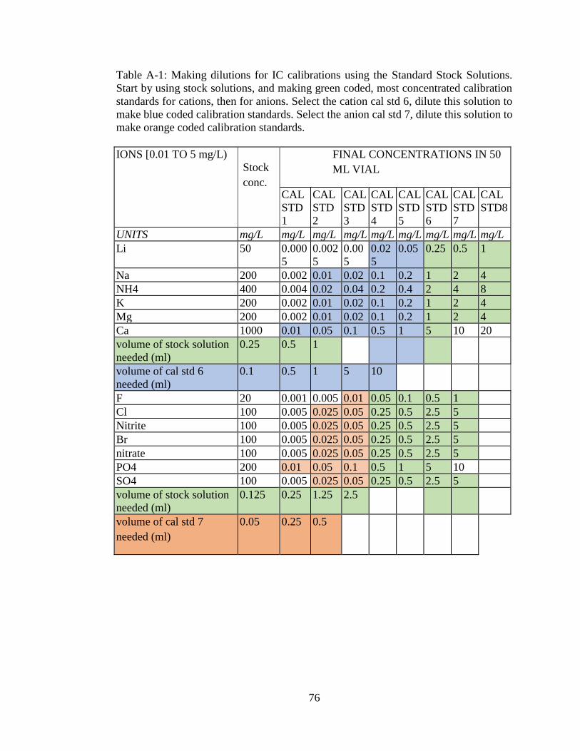
76

Table A-1: Making dilutions for IC calibrations using the Standard Stock Solutions.

Start by using stock solutions, and making green coded, most concentrated calibration

standards for cations, then for anions. Select the cation cal std 6, dilute this solution to

make blue coded calibration standards. Select the anion cal std 7, dilute this solution to

make orange coded calibration standards.

IONS [0.01 TO 5 mg/L)

Stock

conc.

FINAL CONCENTRATIONS IN 50

ML VIAL

CAL

STD

1

CAL

STD

2

CAL

STD

3

CAL

STD

4

CAL

STD

5

CAL

STD

6

CAL

STD

7

CAL

STD8

UNITS mg/L mg/L mg/L mg/L mg/L mg/L mg/L mg/L mg/L

Li 50 0.000

5

0.002

5

0.00

5

0.02

5

0.05 0.25 0.5 1

Na 200 0.002 0.01 0.02 0.1 0.2 1 2 4

NH4 400 0.004 0.02 0.04 0.2 0.4 2 4 8

K 200 0.002 0.01 0.02 0.1 0.2 1 2 4

Mg 200 0.002 0.01 0.02 0.1 0.2 1 2 4

Ca 1000 0.01 0.05 0.1 0.5 1 5 10 20

volume of stock solution

needed (ml)

0.25 0.5 1

volume of cal std 6

needed (ml)

0.1 0.5 1 5 10

F 20 0.001 0.005 0.01 0.05 0.1 0.5 1

Cl 100 0.005 0.025 0.05 0.25 0.5 2.5 5

Nitrite 100 0.005 0.025 0.05 0.25 0.5 2.5 5

Br 100 0.005 0.025 0.05 0.25 0.5 2.5 5

nitrate 100 0.005 0.025 0.05 0.25 0.5 2.5 5

PO4 200 0.01 0.05 0.1 0.5 1 5 10

SO4 100 0.005 0.025 0.05 0.25 0.5 2.5 5

volume of stock solution

needed (ml)

0.125 0.25 1.25 2.5

volume of cal std 7

needed (ml)

0.05 0.25 0.5

77

Table A-2. Sample dilution protocol. Samples were titrated for chloride concentrations

using HACH titration kit and diluted accordingly.

Sample Target dilution Sample Split Wt. Water Wt.

OCSW 1_1000 0.0154 14.9738

CSW1-1 1_10 1.5088 13.7644

CSW1-2 1_1000 0.0156 14.9954

CSW1-3 1_1000 0.0152 14.9954

CSW1-4 1_100 0.1509 14.8188

CSW1-5 1_1000 0.015 15.0072

QV1-1 1_1000 0.0154 15.1095

QV1-2 1_1000 0.0154 15.0286

QV1-3 1_1000 0.0159 15.1456