Genome-wide ancestry of 17th-century enslavedAfricans from the CaribbeanHannes Schroedera,b,1,2, María C. Ávila-Arcosa,c,1, Anna-Sapfo Malaspinasa, G. David Poznikd,Marcela Sandoval-Velascoa, Meredith L. Carpenterc,3, José Víctor Moreno-Mayara, Martin Sikoraa,c, Philip L. F. Johnsone,Morten Erik Allentofta, José Alfredo Samaniegoa, Jay B. Haviserf, Michael W. Deeg, Thomas W. Stafford Jr.h,Antonio Salasi, Ludovic Orlandoa, Eske Willersleva, Carlos D. Bustamantec, and M. Thomas P. Gilberta,2

aCentre for Geogenetics, Natural History Museum of Denmark, University of Copenhagen, 1350 Copenhagen, Denmark; bFaculty of Archaeology, LeidenUniversity, 2300 Leiden, The Netherlands; cDepartment of Genetics, Stanford University, Stanford, CA 94305; dProgram in Biomedical Informaticsand Department of Statistics, Stanford University, Stanford, CA 94305; eDepartment of Biology, Emory University, Atlanta, GA 30322; fSt. MaartenArchaeological Center, Philipsburg, Saint Martin; gResearch Laboratory for Archaeology and the History of Art, University of Oxford, OX1 3QY Oxford,United Kingdom; hAMS 14C Dating Centre, Department of Physics and Astronomy, Aarhus University, 8000 Aarhus, Denmark; and iUnidade de Xenética,Departamento de Anatomía Patolóxica e Ciencias Forenses, and Instituto de Ciencias Forenses, Facultade de Medicina, Universidade de Santiago deCompostela, 15872 Galicia, Spain

Edited by Rick A. Kittles, University of Arizona, Tucson, AZ, and accepted by the Editorial Board February 2, 2015 (received for review November 17, 2014)

Between 1500 and 1850, more than 12 million enslaved Africanswere transported to the New World. The vast majority wereshipped from West and West-Central Africa, but their preciseorigins are largely unknown. We used genome-wide ancient DNAanalyses to investigate the genetic origins of three enslavedAfricans whose remains were recovered on the Caribbean islandof Saint Martin. We trace their origins to distinct subcontinentalsource populations within Africa, including Bantu-speakinggroups from northern Cameroon and non-Bantu speakers livingin present-day Nigeria and Ghana. To our knowledge, thesefindings provide the first direct evidence for the ethnic origins ofenslaved Africans, at a time for which historical records arescarce, and demonstrate that genomic data provide another typeof record that can shed new light on long-standing historicalquestions.

ancient DNA | genomics | slave trade

Historians have long been interested in the origins of themillions of enslaved Africans who were transported to the

Americas, but there is little direct evidence to go on (1, 2).Although much is known about the volume and changing de-mographic trends of the Atlantic slave trade, the African originsof the enslaved remain largely unknown (3). Genome-wide analysesof SNPs provide a powerful tool for estimating individual ancestry,and several studies (e.g., refs. 4 and 5) have shown that they can beused to infer an individual’s geographic origin with great accuracy.In the present study, we used genome-wide data to trace the originsof three enslaved Africans whose remains were recovered in theZoutsteeg area of Philipsburg on the Caribbean island of SaintMartin (Materials and Methods). Previous reports (6) suggest thatthe “Zoutsteeg Three,” as they became known locally, were likelyborn in Africa as opposed to the New World. But they did notreveal where in Africa they originated.Bayesian analysis of individual calibrated radiocarbon dates

suggests that the burials date between A.D. 1660 and 1688 (formore details, see SI Appendix, Section 2). During this period,Saint Martin—like other islands—relied to a large extent onAfrican slave labor, but there are no records about the slaves’origins in Africa. The Transatlantic Slave Trade Database(slavevoyages.org), a large online repository containing in-formation on over 35,000 slaving voyages, lists only a singlevessel that arrived in Saint Martin between A.D. 1650 and 1700,although there were undoubtedly more for which there are norecords. Moreover, the lone entry does not give the African portof embarkation or any information on the slave cargo. Given thelack of documentation, we embarked on a genomic study withthe goal of identifying the genetic origins of the Zoutsteeg Threein Africa.

ResultsInitial shotgun sequencing revealed that the DNA in the sampleswas very poorly preserved (SI Appendix, Section 8). This resultwas expected because DNA preservation in the Caribbean isknown to be poor (7). The fraction of nonredundant readsmapping to the human reference genome varied between 0.3%and 7.6%, and the sequences showed all features typical ofancient DNA, including short average read lengths (∼67 bp),characteristic fragmentation patterns, and an increased fre-quency of apparent C-to-T substitutions toward the 5′ ends ofmolecules (see Table 1 and SI Appendix, Fig. S7). To increasesequencing efficiency and lower cost, we enriched the ancient

Significance

The transatlantic slave trade resulted in the forced movementof over 12 million Africans to the Americas. Although manycoastal shipping points are known, they do not necessarilyreflect the slaves’ actual ethnic or geographic origins. Weobtained genome-wide data from 17th-century remains ofthree enslaved individuals who died on the Caribbean island ofSaint Martin and use them to identify their genetic origins inAfrica, with far greater precision than previously thoughtpossible. The study demonstrates that genomic data can beused to trace the genetic ancestry of long-dead individuals,a finding that has important implications for archeology, es-pecially in cases where historical information is missing.

Author contributions: H.S., M.C.A.A., and M.T.P.G. designed research; H.S., M.S.V., M.L.C.,J.B.H., M.W.D., and T.W.S. performed research; H.S., M.C.A.A., A.S.M., G.D.P., J.V.M.M., M.S.,P.L.F.J., M.E.A., J.A.S., M.W.D., A.S., and L.O. analyzed data; H.S., M.C.A.A., and M.T.P.G.wrote the paper; J.B.H. provided samples; and H.S., E.W., C.D.B., and M.T.P.G.supervised research.

Conflict of interest statement: C.D.B. is the founder of IdentifyGenomics, LLC, and is onthe Scientific Advisory Boards of Personalis, Inc., and Ancestry.com as well as the MedicalAdvisory Board of InVitae. M.L.C. is now the Chief Scientific Officer at IdentifyGenomics,LLC. None of this played a role in the design, execution, or interpretation of experimentsand results presented here.

This article is a PNAS Direct Submission. R.A.K. is a guest editor invited by the EditorialBoard.

Freely available online through the PNAS open access option.

Data deposition: The data reported in this paper have been deposited in the EuropeanNucleotide Archive, www.ebi.ac.uk/ena (project accession no. PRJEB8269). The mappeddata are available upon request.1H.S. and M.C.A.A. contributed equally to this work.2To whom correspondence may be addressed. Email: hschroeder@snm.ku.dk or tgilbert@snm.ku.dk.

3Present address: IdentifyGenomics, LLC, Menlo Park, CA 94305.

This article contains supporting information online at www.pnas.org/lookup/suppl/doi:10.1073/pnas.1421784112/-/DCSupplemental.

www.pnas.org/cgi/doi/10.1073/pnas.1421784112 PNAS Early Edition | 1 of 5

ANTH

ROPO

LOGY

DNA libraries using two recently developed whole-genomecapture methods (8, 9). Following enrichment, we generatedbetween 0.1- and 0.5-fold genome-wide coverage for the threeindividuals, which proved to be sufficient to infer their likelyorigins within Africa.Although the presence of characteristic damage patterns and

short average read lengths suggest that authentic ancient mol-ecules were sequenced, it is possible that some degree of moderncontamination could be present in the data. Therefore, we useda previously published Bayesian method (10) to detect contam-ination and found very low (i.e., <1%) levels overall (see Table 1and SI Appendix, Section 9). We then merged our ancient se-quence data with genotype data from the Human Genome Di-versity Cell Line Panel (HGDP) reference panel (11) and usedprincipal component analysis (PCA) (12) to confirm the indi-viduals’ African ancestry (for more details, see SI Appendix,Section 12). Because of low depth, we randomly sampled a singleallele from both ancient and modern individuals, as done in ref.13. As expected, all three individuals fell within African variationas defined by PC1 and PC2 (SI Appendix, Fig. S17). This clus-tering was retained upon restricting the analysis to sequencesshowing signs of ancient DNA damage (14) (SI Appendix, Fig.S18), indicating that the signal was not driven by modern DNAcontamination.

D-Statistic Test. We then tested the relationships between eachsample (henceforth referred to as STM1, STM2, and STM3) and11 populations from across the world for which whole genomedata were available (15), using a D-test of the form D (chim-panzee, STM; Yoruba, X), where X stands for a populationother than Yoruba (for more details, see SI Appendix, Section

13). We found that the STMs were significantly more closelyrelated to the Yoruba than to any non-African population (Fig.1A), again confirming their African origins. Within Africa, theSTMs appeared significantly more closely related to the Yorubathan to hunter-gatherer populations (San, Mbuti Pygmies). Thiswas not surprising, as the San and the Mbuti were not repre-sented in the transatlantic slave trade. For the Mandenka andDinka, the D-test results were not significant, suggesting thatthese populations are equally closely related to the STMs as arethe Yoruba. The lack of rejection for the Dinka was surprising,as this population—from southern Sudan—is not known to havebeen involved in the Atlantic slave trade (16).

Principal Component Analysis. To refine our assignment withinAfrica, we compared our samples to another reference panel,consisting of genotype data from 11 West African populations(Fig. 1B) (17). We intersected 294,651 sites from this referencepanel with our sequence data (SI Appendix, Section 14) andconducted PCA to determine whether the individuals showedclose affinity to a particular population within the panel. Foreach of the three individuals, we merged the sequence data withthe reference panel genotypes and calculated PC1 and PC2based on the overlapping sites (SI Appendix, Fig. S19). We thencombined the three analyses using Procrustes transformation, asdone in ref. 13. Interestingly, the samples clustered with differentpopulations: Bantu-speaking groups in the case of STM1 (spe-cifically, Bamoun) and non-Bantu–speaking groups for STM2and STM3 (Fig. 1C). We observed similar patterns using theprobabilistic model of population splits and divergence imple-mented in TreeMix (18) (SI Appendix, Fig. S20).

Fig. 1. Genetic affinities of the Zoutsteeg individuals. (A) D-statistic test results for STM3. Error bars correspond to 3 SEs of the D-statistic. Results for STM1and STM2 are plotted in SI Appendix, Fig. S18. (B) Sampling locations for the 11 African populations in our reference panel (17). (C) Procrustes-transformedPCA plot of the Zoutsteeg individuals with African reference panel samples. (D) Ancestry proportions for the Zoutsteeg individuals and those of 188 Africanindividuals in the reference panel, as inferred by ADMIXTURE analysis (19).

2 of 5 | www.pnas.org/cgi/doi/10.1073/pnas.1421784112 Schroeder et al.

ADMIXTURE Analysis. To further explore the genetic ancestry ofthe STMs, we used the maximum-likelihood–based clusteringalgorithm ADMIXTURE (19). When assuming three ancestralpopulations (K = 3), the clusters in the reference panel mirrorthe grouping of individuals in the space defined by PC1 and PC2:a cluster predominating in Bantu-speaking populations, a clusterfor non-Bantu West African populations, and a third restrictedmostly to Kaba, Mada, and Bulala (Fig. 1D). The distribution ofthese components in our samples indicates that STM1 has ahigher proportion of Bantu-specific ancestry, whereas STM2 andSTM3 carry higher proportions of the component prevalentamong the non-Bantu–speaking Yoruba, Brong, and Igbo. No-tably, STM2 also shows a slightly higher proportion of thecomponent prevalent among the Kaba, Mada, and Bulala, per-haps suggesting closer affinity with Chadic or Sudanic speakers(Fig. 1D).

Uniparental Markers. Furthermore, we determined the individuals’mitochondrial DNA (mtDNA) haplogroups and the Y-chromo-some haplogroup of STM1 (SI Appendix, Section 11). ThemtDNAs were assigned to haplogroups L3b1a, L3d1b2, andL2a1f, respectively. Tracing these lineages to particular regionsin Africa is challenging because of their pan-continental distri-bution, which is the result of thousands of years of populationmovements (e.g., the Bantu migrations) and continued gene flow(20–22). Nevertheless, we note that haplogroup L3b1a is one ofthe most common lineages found in the Lake Chad Basin (23).This finding is noteworthy, because the Y-chromosome lineageof this individual (STM1) was identified as belonging to haplo-group R1b1c-V88, which—although quite rare in Africa on thewhole—occurs at extremely high frequency in the Lake ChadBasin, rising to 95% in one population of northern Cameroon (24).

DiscussionTaken together, the genetic data suggest that STM1 may haveoriginated among Bantu-speaking groups in northern Cameroon,whereas STM2 and STM3 more likely originated among non-Bantu speakers living in present-day Nigeria and Ghana. To ourknowledge, these findings provide the first direct evidence forthe ethnic origins of enslaved Africans, with the important caveatthat the modern reference populations might not be the same asthe historical populations who lived in the same locations at thetime of the Atlantic slave trade. Nevertheless, the data suggestthat the Africans who reached Saint Martin were drawn fromdiverse cultures and societies. This finding highlights interestingquestions regarding the formation of Creole communities andthe survival of African cultures in the Americas. Chief amongthese is to what extent Africans were able to maintain Africancultural beliefs and practices following their arrival in the NewWorld (see, for example, refs. 25–27).Genome-wide analyses clearly bear great potential to predict

a person’s place of origin, but we caution that there are also lim-itations. First, accuracy is limited by the number of markers used,although new methods (e.g., ref. 28) are constantly being de-veloped, claiming to achieve greater accuracy using relatively smallsets of makers. Unfortunately, however, many of these methods

rely on called genotypes, which makes them unsuited to low-cov-erage ancient genome studies. Second, accuracy also depends onthe appropriate samples being represented in our reference panels,highlighting the need for more comprehensive sampling and se-quencing of human populations across Africa. Third, tracing theancestry of admixed individuals is more complicated, but advancesare also being made in the study of the ancestral composition ofadmixed genomes (see, for example, refs. 29 and 30). Many ofthese limitations will be overcome, as more data are being gener-ated and new analytical methods are being developed.

ConclusionOur study has several major implications. First, it demonstratesthat it is possible to obtain genome-wide data from poorly pre-served archeological remains found in tropical settings like theCaribbean. This has important implications for future ancientDNA studies in the region, including those addressing pre-Columbian population movements (7). Second, our study under-scores the value of whole-genome capture methods (e.g., ref. 8)for ancient DNA research. These new methods enable us to usesamples that were previously thought to be beyond our reachbecause of their low endogenous DNA contents. Third, our studyhighlights the power of genome-wide analyses for tracing thegenetic origins of long-dead individuals, in this case victims ofthe transatlantic slave trade. As our study shows, genomic datacan provide an alternative kind of record that can help shed lighton long-standing historical questions, in cases where documen-tary records are scarce or unavailable.

Materials and MethodsSamples. The samples used in this study stem from three 17th-century burialsthat were recovered during construction work in the Zoutsteeg area ofPhilipsburg, the capital of the Caribbean island of Saint Martin in 2010.Skeletal analysis suggested that the individuals—two males and onefemale—were of African ancestry and that they had been aged between 25and 40 y at the time of death. The most striking feature of the skeletonswas that all three had culturally modified teeth (SI Appendix, Section 1). Similartypes of dental modification are known to have been practiced by differentgroups in Africa but a look at the ethnographic literature (e.g., refs. 31 and32) suggests that they cannot be used to infer points of origin or specific“tribal” affiliations.

DNA Extraction and Library Preparation. DNA was extracted from tooth rootsusing a silica-based method (33) and eluted in 60 μL EB. Thirty microliters ofextract were then built into Illumina libraries using the NEBNext DNASample Prep Master Mix Set 2 (New England Biolabs) and Illumina-specificadapters (34) following the manufacturer’s instructions, with some minorchanges to the protocol (SI Appendix, Section 3). The remaining 30 μL ofDNA extract were built into Illumina libraries using a single-stranded librarypreparation protocol, as described in ref. 35 but without first removingdeoxyuracils. Both sets of libraries were amplified and indexed in 50-μL PCRreactions, purified, quantified, and pooled for sequencing (for more details,see SI Appendix, Section 3).

Whole-Genome Capture.Weused twowhole-genome capturemethods to enrichtwo sets of aDNA libraries in their human DNA content. Both methods make useof biotinylated RNA probes transcribed from genomic DNA libraries to capturethe human DNA in the aDNA libraries. The first method, which we refer to as

Table 1. Modeled radiocarbon dates and sequencing results for the Zoutsteeg Three

Sample Modeled 14C age* Sex† Nuclear coverage Contamination (%)‡ Damage (%)§ Mt coverage Mt haplogroup Y haplogroup

STM1 A.D. 1660–1688 M 0.3× 0.63 16.8 641× L3b1a R1b1c-V88STM2 A.D. 1660–1688 M 0.1× 0.22 23.2 543× L3d1b —

STM3 A.D. 1660–1688 F 0.5× 0.15 14.9 651× L2a1f —

*Modeled age range of the samples based on Bayesian analysis of individual calibrated radiocarbon dates.†Biological sex inferred from the ratio of reads mapping to X and Y chromosomes (44).‡Likelihood-based contamination estimate based on mtDNA reads (10).§Frequency of C-to-T misincorporations at 5’ ends of sequencing reads.

Schroeder et al. PNAS Early Edition | 3 of 5

ANTH

ROPO

LOGY

WISC (Whole Genome In-Solution Capture), was carried out as described in ref. 8,using home-made biotinylated RNA probes. For the second capture experiment,we used the MYbait Human Whole Genome Capture Kit (MYcroarray), follow-ing the manufacturer’s instructions (9). Following the capture experiments, theenriched libraries were amplified again, purified, quantified, and sequenced onan Illumina HiSeq 2000 (for more details, see SI Appendix, Section 4).

Data Processing. We used AdapterRemoval (36) to trim adapter sequencesand to remove adapter dimers and low quality reads (SI Appendix, Section 5).Filtered fastq files were mapped to the human reference genome versionhg18 and hg19, but replacing the mitochondria with the revised CambridgeReference Sequence (37). Mapping was done using BWA v0.7.5a-r405 (38),keeping only reads with mapping quality 30 and above. Duplicate readswere removed using SAMtools’ (39) rmdup function. BAM files from dif-ferent runs were merged using SAMtools merge. Sequencing error rateswere estimated to be on the order of 0.3% (SI Appendix, Section 6). Map-Damage2 (40) was used to rescale the quality of bases that had a mismatchto the reference likely derived from damage (for more details, see SI Ap-pendix, Section 7).

mtDNA and Y-Chromosome Haplogroups. mtDNA haplogroups were deter-mined by recovering reads mapping to the revised Cambridge ReferenceSequence (37) from the BAM files and generating a consensus sequence andlist of variants using SAMtools/BCFtools v0.1.19 (38). Indels and hotspotmutations were excluded from analysis. Haplogroups were determined us-ing HaploGrep (41). The maximum parsimony tree (SI Appendix, Fig. S12)was built using mt-Phyl (eltsov.org). The Y-chromosome haplogroup forSTM1 was determined by assembling a panel of phylogenetically in-formative SNPs, with emphasis on those lineages previously reported tooccur at appreciable frequencies within Africa. For more details, see SI Ap-pendix, Section 11.

Reference Panels. For the genome-wide analyses we used three previouslypublished reference data sets, including: (i) a dataset of 11 modern genomesused in ref. 15, (ii) genotype data for 854 unrelated individuals from 52worldwide populations from the HGDP reference panel described in ref. 11,and (iii) a reference panel consisting of 146 individuals from 11 sub-Saharanpopulations genotyped on the Affymetrix 500k array set (17). Beforemerging with the aDNA sequence data, we randomly sampled one allele ateach site and for each individual in the reference panel and made such sitehomozygous for the drawn allele, as described in ref. 13. For more details,see SI Appendix, Section 12.

Principal Component Analysis. For each file containing the genotypes of thesample and reference panels, we ran smartpca (EIGENSOFT v4.0) (42) toperform PCA. Eigenvectors were plotted independently for each datasetusing RStudio (www.rstudio.com). To visualize the three samples in a singlePCA plot we used Procrustes transformation as done in ref. 13. We transformed

the first two PCs calculated for each intersected dataset to match the reference-only PC1 and PC2. When transforming the PCs, the ancient individual wasexcluded. The configuration of transformed PC1 and PC2 was then applied tothe ancient individuals, and transformed coordinates were overlaid on thereference-only PC1 and PC2 plot (Fig. 1C). For more details, see SI Appendix,Section 14.

TreeMix Analysis. We used the probabilistic model of population splits anddivergence implemented in TreeMix (18) to infer ancestry graphs (SI Ap-pendix, Fig. S20). As input we used estimated allele frequencies for oursamples and the populations in our reference panel (17). For each datasetwe ran 100 bootstraps with random seeds and with the -noss and -global flags todisable sample size correction, and perform a round of global rearrangements ofthe graph, respectively. Additionally, the number of SNPs per block was calcu-lated for each dataset to allow ∼1,000 blocks. Finally, the root of the tree was setto Xhosa. For more details, see SI Appendix, Section 15.

ADMIXTURE Analysis. We used the maximum-likelihood–based clustering algo-rithm ADMIXTURE (19) to estimate the genetic structure in our merged dataset(for more details, see SI Appendix, Section 16). We first estimated the cross-validation error with the -cv flag for K values between 1 and 6. This analysisrevealed that the CV error increased with K, probably reflecting the very low Fstbetween the populations in the reference panel. For K = 4 to K = 6 we ran 100replicates using a random seed and kept the Q (ancestral cluster proportions)and P (inferred ancestral cluster allele frequencies) matrices from the run withthe best log likelihood. We used the P matrix from each K to estimate the mostlikely cluster proportions in the ancient samples as was done in ref. 43. SI Ap-pendix, Fig. S21 shows the converged runs from K = 2 to K = 6 for STM1, STM2,and STM3 and 11 sub-Saharan populations in our reference panel (17).

ACKNOWLEDGMENTS. We thank the staff at the Danish National High-throughput Sequencing Centre for technical support; P. F. Campos,M. Rasmussen, T. Korneliussen, F. Sánchez-Quinto, P. Skoglund, A. Moreno-Estrada, F. Mendez, and P. Underhill for their various input and helpfuldiscussions; and J.S. Handler for reading earlier drafts of the paper and pro-viding valuable comments. The Centre for Geogenetics is funded by theDanish National Research Foundation (DNRF94). This work was supportedin part by Marie Curie Fellowships from the Directorate General for Researchand Innovation of the European Commission FP7/2007-2013/236435 and317184 (to H.S. and M.E.A.); Grants FP7/2007-2013/269442 and 319209 fromthe European Research Council (to H.S. and M.E.A.); National Science Foun-dation Grants DMS-1201234 and DGE-1147470 (to M.C.A.A. and G.D.P.);Swiss National Science Foundation Fellowship PBSKP3-143529 (to A.S.M.);National Institute of Health Grants NRSA 5F32HG007342 and K99 GM104158(to M.L.C. and P.L.F.J.); Leverhulme Early Career Fellowship ECF-2012-123(to M.W.D.); Ministerio de Ciencia e Innovación Grant SAF2011-26983 (toA.S.); the “Plan Galego IDT” EM 2012/045 (to A.S.); “Sistema UniversitarioGallego-Modalidad REDES” Grant 2012-PG226 from the Xunta de Galicia(to A.S.); Lundbeck Foundation Grant R52-A5062 (to M.T.P.G.); and DanishCouncil for Independent Research Grant 10-081390 (to M.T.P.G.).

1. Palmer CA (1995) From Africa to the Americas: Ethnicity in the early black commu-

nities of the Americas. J World Hist 6(2):223–236.2. Morgan PD (1997) The cultural implications of the Atlantic slave trade: African re-

gional origins, American destinations and new world developments. Slavery Abol

18(1):122–145.3. Northrup D (2000) Igbo and Myth Igbo: Culture and ethnicity in the Atlantic world,

1600–1850. Slavery Abol 21(3):1–20.4. Novembre J, et al. (2008) Genes mirror geography within Europe. Nature 456(7218):

98–101.5. Lao O, et al. (2008) Correlation between genetic and geographic structure in Europe.

Curr Biol 18(16):1241–1248.6. Schroeder H, et al. (2014) The Zoutsteeg Three: Three new cases of African types of

dental modification from Saint Martin, Dutch Caribbean. Int J Osteoarchaeol 24(6):

688–696.7. Lalueza-Fox C, Gilbert MT, Martínez-Fuentes AJ, Calafell F, Bertranpetit J (2003) Mi-

tochondrial DNA from pre-Columbian Ciboneys from Cuba and the prehistoric colo-

nization of the Caribbean. Am J Phys Anthropol 121(2):97–108.8. Carpenter ML, et al. (2013) Pulling out the 1%: Whole-genome capture for the tar-

geted enrichment of ancient DNA sequencing libraries. Am J Hum Genet 93(5):

852–864.9. MYcroarray (2013) MYbaits Manual. Available at www.mycroarray.com/pdf/

MYbaits-manual.pdf. Accessed March 1, 2014.10. Fu Q, et al. (2013) A revised timescale for human evolution based on ancient mito-

chondrial genomes. Curr Biol 23(7):553–559.11. Rosenberg NA (2006) Standardized subsets of the HGDP-CEPH Human Genome Di-

versity Cell Line Panel, accounting for atypical and duplicated samples and pairs of

close relatives. Ann Hum Genet 70(Pt 6):841–847.

12. Patterson N, Price AL, Reich D (2006) Population structure and eigenanalysis. PLoSGenet 2(12):e190.

13. Skoglund P, et al. (2012) Origins and genetic legacy of Neolithic farmers and hunter-gatherers in Europe. Science 336(6080):466–469.

14. Skoglund P, et al. (2014) Separating endogenous ancient DNA from modern daycontamination in a Siberian Neandertal. Proc Natl Acad Sci USA 111(6):2229–2234.

15. Meyer M, et al. (2012) A high-coverage genome sequence from an archaic Denisovanindividual. Science 338(6104):222–226.

16. Diouf S (2013) Servants of Allah: African Muslims Enslaved in the Americas (New YorkUniv Press, New York, NY).

17. Bryc K, et al. (2010) Genome-wide patterns of population structure and admixture inWest Africans and African Americans. Proc Natl Acad Sci USA 107(2):786–791.

18. Pickrell JK, Pritchard JK (2012) Inference of population splits and mixtures fromgenome-wide allele frequency data. PLoS Genet 8(11):e1002967.

19. Alexander DH, Novembre J, Lange K (2009) Fast model-based estimation of ancestryin unrelated individuals. Genome Res 19(9):1655–1664.

20. Salas A, et al. (2004) The African diaspora: mitochondrial DNA and the Atlantic slavetrade. Am J Hum Genet 74(3):454–465.

21. Salas A, Carracedo A, Richards M, Macaulay V (2005) Charting the ancestry of AfricanAmericans. Am J Hum Genet 77(4):676–680.

22. Ely B, Wilson JL, Jackson F, Jackson BA (2006) African-American mitochondrial DNAsoften match mtDNAs found in multiple African ethnic groups. BMC Biol 4:34.

23. Cerezo M, �Cerný V, Carracedo Á, Salas A (2011) New insights into the Lake Chad Basinpopulation structure revealed by high-throughput genotyping of mitochondrial DNAcoding SNPs. PLoS ONE 6(4):e18682.

24. Cruciani F, et al. (2010) Human Y chromosome haplogroup R-V88: A paternal geneticrecord of early mid Holocene trans-Saharan connections and the spread of Chadiclanguages. Eur J Hum Genet 18(7):800–807.

4 of 5 | www.pnas.org/cgi/doi/10.1073/pnas.1421784112 Schroeder et al.

25. Mintz SW, Price R (1992) The Birth of African-American Culture: An AnthropologicalPerspective (Beacon Press, Boston, MA).

26. Midlo Hall G (2007) Slavery and African Ethnicities in the Americas: Restoring theLinks (Univ of North Carolina Press, Chapel Hill, NC).

27. Lovejoy PE, ed (2009) Identity in the Shadow of Slavery (Continuum, London, UK).28. Elhaik E, et al.; Genographic Consortium (2014) Geographic population structure

analysis of worldwide human populations infers their biogeographical origins. NatCommun 5:3513.

29. Yang WY, Novembre J, Eskin E, Halperin E (2012) A model-based approach foranalysis of spatial structure in genetic data. Nat Genet 44(6):725–731.

30. Moreno-Estrada A, et al. (2013) Reconstructing the population genetic history of theCaribbean. PLoS Genet 9(11):e1003925.

31. von Jehring H (1882) Die künstliche Deformierung der Zähne. Z Ethnol 14:213–262.32. Lignitz H (1919-1922) Die künstlichen Zahnverstümmelungen in Afrika im Lichte der

Kulturkreisforschung. Anthropos 14-15:891–943.33. Rohland N, Hofreiter M (2007) Ancient DNA extraction from bones and teeth. Nat

Protoc 2(7):1756–1762.34. Meyer M, Kircher M (2010) Illumina Sequencing Library preparation for highly multi-

plexed target capture and sequencing. Cold Spring Harb Protoc 2010(6):pdb.prot5448.35. Gansauge MT, Meyer M (2013) Single-stranded DNA library preparation for the se-

quencing of ancient or damaged DNA. Nat Protoc 8(4):737–748.

36. Lindgreen S (2012) AdapterRemoval: Easy cleaning of next-generation sequencing

reads. BMC Res Notes 5:337.37. Andrews RM, et al. (1999) Reanalysis and revision of the Cambridge reference se-

quence for human mitochondrial DNA. Nat Genet 23(2):147.38. Li H, Durbin R (2009) Fast and accurate short read alignment with Burrows-Wheeler

transform. Bioinformatics 25(14):1754–1760.39. Li H, et al.; 1000 Genome Project Data Processing Subgroup (2009) The Sequence

Alignment/Map format and SAMtools. Bioinformatics 25(16):2078–2079.40. Jónsson H, Ginolhac A, Schubert M, Johnson PL, Orlando L (2013) mapDamage2.0:

Fast approximate Bayesian estimates of ancient DNA damage parameters. Bio-

informatics 29(13):1682–1684.41. Kloss-Brandstätter A, et al. (2011) HaploGrep: A fast and reliable algorithm for au-

tomatic classification of mitochondrial DNA haplogroups. Hum Mutat 32(1):25–32.42. Price AL, et al. (2006) Principal components analysis corrects for stratification in ge-

nome-wide association studies. Nat Genet 38(8):904–909.43. Sikora M, et al. (2014) Population genomic analysis of ancient and modern genomes

yields new insights into the genetic ancestry of the Tyrolean Iceman and the genetic

structure of Europe. PLoS Genet 10(5):e1004353.44. Skoglund P, et al. (2013) Accurate sex identification of ancient human remains using

DNA shotgun sequencing. J Arch Sci 40:4477–4482.

Schroeder et al. PNAS Early Edition | 5 of 5

ANTH

ROPO

LOGY

1 of 47

Supplementary Information

Genome-wide ancestry of 17th-century enslaved Africans from the Caribbean

H. Schroeder1,2, M.C. Ávila-Arcos1, A.-S. Malaspinas, G.D. Poznik, M. Sandoval-Velasco, M.L. Carpenter,

J.V. Moreno-Mayar, M. Sikora, P.L.F. Johnson, M.E. Allentoft, J.A. Samaniego, J.B. Haviser, M.W. Dee, T.W. Stafford, Jr., A. Salas, L. Orlando, E. Willerslev, C.D. Bustamante, M.T.P. Gilbert2

1These authors contributed equally to this work. 2To whom correspondence should be addressed. E-mail: hschroeder@snm.ku.dk; tgilbert@snm.ku.dk

2 of 47

Table of Contents

1 Samples and archeological context ............................................................................................................... 3

2 Radiocarbon dating and Bayesian analysis of radiocarbon dates ................................................................... 4

3 DNA extraction and library preparation ......................................................................................................... 5

4 Whole genome capture and sequencing ....................................................................................................... 6

5 Sequence data filtering and mapping ........................................................................................................... 7

6 Relative sequencing/alignment error rates .................................................................................................... 7

7 mapDamage analysis .................................................................................................................................... 9

8 Characterization of DNA preservation ........................................................................................................... 9

9 Contamination estimates .............................................................................................................................. 11

10 Determining the biological sex of the Zoutsteeg Three ................................................................................ 11

11 Mitochondrial DNA and Y-chromosome analysis ......................................................................................... 11

12 Genotype reference panels ......................................................................................................................... 14

13 D-statistic tests ........................................................................................................................................... 15

14 Principal component analysis ...................................................................................................................... 15

15 TreeMix analysis ......................................................................................................................................... 16

16 Admixture analysis ..................................................................................................................................... 16

Supplementary Figures .................................................................................................................................... 17

Supplementary Tables ..................................................................................................................................... 38

References and Notes ...................................................................................................................................... 44

3 of 47

1 Samples and archeological context

Construction work in the Zoutsteeg area of Philipsburg on the Caribbean island of Saint Martin in March 2010 revealed three articulated human skeletons. The remains were found at a depth of ca. 140-160 cm in a layer of fine loose beach sand. The layer above the burials contained several modern, 18th- and 19th-century artifacts including ceramics, red brick fragments and two unidentified iron fragments. The layer with the burials contained several other artifacts, including several pieces of late 17th-century ceramics (slipware, porcelain, salt-glaze stoneware, lead-glaze earthenware and coarse earthenware) and several glass bottle fragments including two square bottle bases with rough pontil scars (Fig. S1). In addition, two modified green stones and an almost intact conch shell were found in association with the second skeleton. Whether or not these artifacts were deliberately placed in the graves is difficult to say. However, it should be noted that pottery shards, glass bottle fragments and other seemingly insignificant objects were a common feature of African-American burial traditions, as were conch shells, especially in the Caribbean (1, 2).

Age, sex and ancestry estimates were made using standard osteological criteria, including cranial and pelvic morphology, dental eruption and wear, cranial suture and epiphyseal closure, and overall robusticity (3, 4). The remains belonged to three adults of probable African ancestry, aged between 25 and 40 years at the time of death. The first skeleton (STM1) belonged to a 25-30 year-old probable male. The skeleton was relatively well preserved with over 40% of the bones present, some of which showed clear signs of treponemal infection. Skeleton number two (STM2) belonged to an older male who would have been approximately 35-40 years old at the time of death. The skeleton was nearly complete with over 80% of the bones preserved. The skull, however, was only partially preserved, and large parts of the right side of the skull were missing. The size of the long bones suggests that this individual had been a very tall person, with a calculated stature of about 190 cm. The third skeleton (STM3) belonged to that of a female who died when she was 30-35 years of age. Her skeleton was also relatively well preserved with over 60% of the bones present. Unfortunately, however, the mandible was missing.

The most striking feature of the skeletons was that their teeth had been intentionally modified. In case of STM1, the occlusal edge of the two central upper incisors had been filed down horizontally, save for the distal extremities, which had been left and cut vertically (Fig. S2). The lateral upper incisors had also been filed on the distal side, creating a pointed shape. The lower incisors were all missing but it is possible that they had also been modified. In case of STM2, the upper incisors had been chipped on both the mesial and distal sides, resulting in a pointed shape (Fig. S3). The two left lower incisors were missing but the other two had also been modified to create a pointed shape and it seems safe to assume that all four had been originally modified the same way. For STM3, the whole mandible and both central upper incisors were missing but both upper lateral incisors were still present and had also been modified to produce a pointed shape (Fig. S4). Although the central incisors were missing, it can be assumed that they had also been filed, as it was very uncommon to modify the lateral incisors alone (5-8).

Similar types of dental modification are known from Africa but it is difficult to be more specific because the designs, especially some of the more common ones, were used by several groups (35-39). The W-shaped pattern used in case of STM2 (Fig. S3) appears to have been fairly common, as it has been reported from several parts of Africa (5-8). The design used in case of STM1 (Fig. S2) seems to have been less common but it was also used by several groups, including the Bakongo, the Loango and others (6). Unfortunately, the dentition of STM3 was incomplete so that it was not possible to identify a specific pattern. But in any case it seems clear that, as Witkin (10) rightly points out, the modifications on their own cannot be used to suggest points of origin or specific tribal affiliations.

4 of 47

To further investigate the origins of the Zoutsteeg Three, Schroeder et al. (11) used strontium isotope analyses, a technique that had been used previously to identify African-born individuals at other archeological sites in the Americas (e.g., 12). The strontium values for the Zoutsteeg Three were clearly distinct so as to suggest that they originated in different parts of Africa but as with previous studies (e.g., 12, 13) it was not possible to pinpoint where in Africa they had originated (11). In summary, neither the patterns of dental modification nor the isotope values could be used to suggest possible points of origin in case of the Zoutsteeg Three which is why we embarked on the genomic analysis of the remains.

2 Radiocarbon dating and Bayesian analysis of radiocarbon dates

We radiocarbon dated the skeletons to determine the precise date of burial. However, this was complicated by the fact that calibrating radiocarbon dates post 1500 AD generally results in broad calendar date ranges due to the shape of the calibration curve (14). To obtain more precise date ranges we incorporated the dates into a Bayesian model that included independent prior information regarding the burials, as well as an approximation for the turnover rate of bone collagen, i.e. 10 ± 5 years. That way, we obtained a calibrated date range of 1660-1688 AD (95.4% probability) as the most likely date of burial. The Transatlantic Slave Trade Database lists only a single slaving voyage (15) that arrived in Saint Martin during that period although there were undoubtedly others that went unrecorded. Unfortunately, however, the records do not contain any information regarding the place of slave purchase, let alone the actual origins of the enslaved.

Radiocarbon dating

The bone samples were dated at the W. M. Keck Carbon Cycle AMS facility of the University of California, Irivine (UCIAMS). Sample preparation and collagen extraction were done following established protocols (16). The bone samples were initially cleaned by removing adhering sediment and the outer 1 mm layer of the bone. Subsequently, approximately 200-400 mg of bone were broken up and left to demineralize in 0.5 N HCl at 5°C for 36 hr. Following a brief alkali bath in 0.1 N NaOH at room temperature to remove humates, the resulting residue was rinsed several times in ultrapure water, and then gelatinized for 12 hr at 70°C in 0.01N HCl. The gelatin solution was then pipetted into pre-cleaned Amicon Centriprep® 30 ultrafilters (30 kD MWCO) and centrifuged three times for 30 min, diluted with distilled H2O and centrifuged three more times for 30 min to desalt the solution. The filtered collagen solution was then freeze-dried and weighed to determine percent yield. For 14C dating, approx. 2.5 mg of collagen was combusted at 900°C in vacuum-sealed quartz tubes with CuO and Ag wire. The sample CO2 was then reduced to graphite at 550°C using H2 and a Fe catalyst, with reaction water drawn off with Mg(ClO4)2. Graphite samples were pressed into targets in Al boats and loaded on the target wheel for AMS analysis. The 14C ages were δ13C-corrected for mass dependent fractionation with measured 14C/13C values, and compared with samples of Pleistocene horse bone (background, >48 14C kyr BP), middle Holocene pinniped bone (~6500 14C BP), late 1800 AD cow bone, and OX-1 oxalic acid standards for calibration. Stable isotope ratios and atomic C/N ratios were determined using a Fisons NA1500NC elemental analyzer/Finnigan Delta Plus isotope ratio mass spectrometer with a precision of <0.1‰ for δ13C and δ15N. The radiocarbon and stable isotope results are listed in Table S1. All three bone samples yielded acceptable C/N ratios. Radiocarbon dates were calibrated using OxCal v4.2.3 (17) and the IntCal13 calibration curve (14).

Bayesian modeling of the radiocarbon results

Radiocarbon dates are never single-year estimates but probability density functions in absolute time, usually expressed as 68% (1σ) or 95% (2σ) ranges. A powerful tool for analyzing such

5 of 47

probability functions is Bayesian statistical modeling (18). This approach allows radiocarbon data to be combined with independent chronological information, such as ordering from stratigraphy. The modeling process often generates probability functions of improved precision.

In the case of these three burials, the independent or prior information is fundamental to the refinement of the dating. The individual calibrated dates for each sample essentially take the form of tri-modal distributions, with some probability allocated to each of the 17th, 18th and 20th centuries. However, archaeological excavation has previously established that the burials predate the foundation of the town of Philipsburg (1735 AD). By incorporating this information in a Bayesian model using the program OxCal v4.2.3 (17), and recalculating the resulting probability estimates, it is clear that only the 17th-century portion of the original calibrations is relevant. Further information may be included in the modeling to improve the dating precision or test archaeological hypotheses. For example, it is widely accepted (e.g., 19), that the radiocarbon concentration of collagen (the fraction extracted for dating) is the result of several years metabolism. Indeed, a the bone collagen of adults in their twenties and thirties is thought to be approximately 10 years older than the individuals themselves (20). This minor offset is accounted for here using a Normal distribution (10 ±5 years). Finally, the impact of the relative ordering of the burials can also be assessed. Fig. S5 shows the date ranges produced if they are assumed to have occurred independently over an unknown period of time, and also gives the results if they are assumed to have occurred in the same year.

3 DNA extraction and library preparation

DNA extraction

DNA was extracted from tooth roots, using a modified silica extraction method (21). All DNA extraction and library preparation steps were performed in dedicated clean laboratories at the Centre for Geogenetics in Copenhagen, Denmark. The samples were initially cleaned by removing any adhering sediment and the surface layer using Dremel tool fitted with a disposable rotating disc. The samples were then wiped with a tissue dipped in 10% bleach solution and UV-irradiated for 2 min on each side to further reduce the amount of surface contaminants and inhibitors. Subsequently, the tooth root was cut off and ground to a coarse powder using a ball mill. Between 200-300 mg of root powder was then weighed into 5 ml Eppendorf tubes and digested overnight at 37°C in 4 ml of an EDTA-based digestion buffer containing 0.25 mg/mL Proteinase K. The digests were then purified using a silica method as described in (21) but with the following modifications. During the binding step, we used 50 µl of silica suspension and samples were eluted in 60 µl TET buffer.

Library preparation

Thirty µl of each of the DNA extracts were built into NGS libraries using the NEBNext DNA Sample Prep Master Mix Set 2 (New England Biolabs Inc., Beverly, MA, USA) and Illumina specific adapters (22). The libraries were prepared according to manufacturer’s instructions, with the following modifications. The initial nebulization step was skipped because of the fragmented nature of ancient DNA (aDNA). End-repair was performed in 50 µl reactions using 30 µl of DNA extract. The reactions were incubated for 20 min at 12°C and 15 min at 37°C, purified using QIAGEN MinElute spin columns (Hilden, Germany) and 10X PN buffer, and eluted in 30 µl EB. The adapter ligation step was performed in 50 µl reactions using 30 µl of end-repaired DNA and Illumina-specific adapters (22). The reactions were incubated for 15 min at 20°C and purified using QIAGEN MinElute columns and 5X PB before being eluted in 25 µl EB. The adaptor fill-in step was performed in a reaction of 30 µl and incubated for 20 min at 37°C followed by 20 min at 80°C to inactivate the Bst polymerase. The entire DNA libraries were then amplified and indexed in a 50 µl PCR reactions, containing 1X KAPA HiFi HotStart Uracil+ ReadyMix (KAPA

6 of 47

Biosystems, Woburn, MA, USA) and 200 nM of each of Illumina’s Multiplexing PCR primer inPE1.0 (5’- AATGATACGGCGACCACCGAGATCTACACTCTTTCCCTACACGAC GCTCTT CCGATCT) and a custom-designed index primer with a six nucleotide index (5’- CAAGCAGAAGACGGCATAC GAGATNNNNNNGTGACTGGAGTTC). Thermocycling conditions were as follows: 1 min at 94°C, followed by 8-12 cycles of 15 sec at 94°C, 20 sec at 60°C, and 20 sec at 72°C, and a final extension step of 1 min at 72°C. The optimal number of cycles was determined by qPCR, as done in (22). The amplified libraries were then purified using Agencourt AMPure XP beads (Beckman Coulter, Krefeld, Germany) and quantified on an Agilent 2100 bioanalyzer (Agilent Technologies, Palo Alto, CA, USA) run in High Sensitivity mode.

The remaining 30 µl of the DNA extracts were also built into Illumina libraries using a single-stranded library preparation protocol that has been specifically designed for the sequencing of ancient or damaged DNA (23). The libraries were prepared as described in (23) but without first removing deoxyuracils.

As expected, ‘shotgun’ yields were consistently higher for the libraries prepared with the single-stranded method than those prepared with NEB’s NEBNext library preparation kit (see Tables S2 and S3). This is mainly due to the fact that the single-stranded method is entirely devoid of purification steps that are an integral part of NEB’s library preparation protocol. Further, the single-stranded method is able to incorporate DNA molecules with single-strand breaks into libraries, which tend to be lost with the double-stranded method, as described in (23). This is also reflected in the shorter average read length for the single-stranded libraries (see Table S3).

4 Whole genome capture and sequencing

We enriched the endogenous component of the three double-stranded and the three single-stranded libraries using two different whole genome target enrichment schemes. Both methods make use of biotinylated RNA probes transcribed from genomic DNA libraries to capture the human DNA in the aDNA libraries. The first method, which we refer to as WISC (for Whole Genome In Solution Capture), was carried out as described in (24) using homemade biotinylated RNA probes. For the second capture experiment, we used the MYbait Human Whole Genome Capture Kit (MYcroarray, Ann Arbor, MI). The libraries were captured according to manufacturer’s instructions (25). The captured libraries were amplified for 10-20 cycles using primers IS5 (5’-AATGATACG GCGACCACCGA) and IS6 (5’-CAAGCAGAAGACGGCA TACGA) and the same PCR set-up conditions as above. Subsequently, the libraries were purified using Agencourt AMPure XP beads, quantified using an Agilent 2100 bioanalyzer, pooled in equimolar amounts, and sequenced on six lanes of an Illumina HiSeq 2000 run in 100 SR mode. Base-calling was performed using the Illumina software CASAVA 1.8.2.

The sequencing results for both types of libraries, before and after capture, are listed in Tables S2 and S3. Whole genome capture led to a significant gains in library yields overall, although we obtained slightly better results using MYbait’s Human Whole Genome Capture Kit (25) than WISC (24). Further, it is worth pointing out that both whole genome target enrichment methods performed better on double- than on single-stranded libraries. For double-stranded libraries we achieved up to 6-fold enrichment with MYbait’s Human Whole Genome Capture Kit (25) and up to 4-fold enrichment using WISC (24). In contrast, for the single-stranded libraries maximum enrichment was only 2-fold. This difference can be explained by the fact that hybridization-based capture methods, like those employed here, bias against the shorter fragments that are present in single-stranded libraries. This is reflected in the dramatic increase in average read lengths after capture. We obtained similar results with a larger set of samples (26).

7 of 47

5 Sequence data filtering and mapping

We used AdapterRemoval (27) to trim adapter sequences on the 3’ end of single end reads and to exclude adapter dimers, low quality stretches and N’s at the ends of reads. The program was run in default mode, allowing for up to three mismatches between reads and the adapter sequence. Filtered fastq files were then mapped to the human reference genome version hg18 and hg19 but replacing the mitochondria with the revised Cambridge Reference Sequence (rCRS). Mapping was done using BWA version 0.7.5a-r405 (28) keeping only reads with mapping quality ≥30. Clonal reads were removed using SAMtools’ (29) rmdup function, and reads reported as having alternative mapping coordinates discarded by controlling for XA, XT and X0 tags. Endogenous content was estimated dividing the number of reads retained after filtering by the total number of trimmed reads. Bam files from different runs were merged using SAMtools (29) merge. MapDamage2 (30) was used to generate fragmentation and damage plots (see Fig. S7) and to rescale the quality of bases that had a mismatch to the reference likely derived from damage (see also section 7).

Filtering damaged reads using PMDtools To assess the effect of potential contamination on the results, we used PMDtools (31) to filter bam files and retain only reads showing signs of aDNA damage. We only retained reads with a pmd (post-mortem damage) score ≥3 and intersected them with the reference panel (see section 12) to assess if the PCA displayed the same clustering of the samples as with the unfiltered set (see section 14). Following filtering we retained 58,078, 59,994, and 103,464 reads for STM1, STM2, and STM3, respectively. The results of the PC analysis restricted to damaged reads only are shown in Fig. S18.

6 Relative sequencing/alignment error rates

We estimated overall error rates (sequencing errors or post-mortem damage) by two different methods: 1) by using an approach similar to the one used by Reich et al. in (32) and 2) by making use of the Y-chromosome sequence data obtained for STM1.

Overall and type-specific error rate estimates

The first method makes use of a high-quality human genome and the chimpanzee sequence as an outgroup and works on the assumption that any given human sample should have on average the same number of derived alleles compared to the chimpanzee sequence. The numbers of derived alleles are counted from the high quality genome and it is assumed that any excess of derived alleles (compared to the high quality genome) observed in our sample is due to errors. Since the high-quality genome has errors as well, the estimated error rate can roughly be understood as the excess error rate relative to the error rate of the high quality genome. Overall error rates were estimated using a method of moments estimator, while the type specific error rates were estimated based on a maximum likelihood approach as described in (33).

We used NA12778 from the 1000 Genomes Project (34) as the high-quality genome and the chimpanzee genome (pantro2 from the hg19 multiz46) to determine the ancestral allele. The high quality genome was filtered with minimum base quality 35 and minimum mapping quality 35. For STM1, STM2, and STM3, we removed all reads with a mapping quality below 30 and all bases with a quality score below 20 (see section 5).

The estimated error rates are shown in Figure S6. Each bar represents a type-specific error. Overall error rates are 0.3%, 0.6%, and 0.3% for STM1, STM2, and STM3, respectively. These estimates are ca.10 times higher than those reported for modern genomes but they are comparable to previously reported error rates for other ancient genomes including the Siberian Mal’ta genome (0.3% overall) (35) and the Native American Anzick genome (0.8%) (36). The main reason for

8 of 47

the increased error rates in ancient genomes is the expected increase C→T and G→A transitions cause by ancient DNA damage (see section 7). Indeed, when excluding C→T and G→A errors, the average error rate of the ancient genomes is comparable to those of modern genomes (e.g., 34).

Leveraging the Y-chromosome to estimate the error rate

Upon identifying the point of divergence of STM1’s Y-chromosome lineage from the known phylogeny (see section 12), we gained an expectation for both the genotypes STM1 carried across the vast majority of known variant sites and for the number of derived alleles he likely carried at unknown sites of variation. We leveraged this information to empirically estimate the genotype error rate, where we define an error as any call that does match the true genotype of STM1. These include both sequencing errors and DNA damage—mutations that have arisen due to post-mortem deamination events.

Elsewhere in the genome, there is no ground-truth. Each locus has its own genealogical tree, and any locus within an individual has the potential to diverge from haplotype reference panels or to represent a previously unobserved recombinant haplotype. Consequently, we cannot know with certainty what the genotypes “should” be at known sites, nor how many novel variants to expect. In contrast, the entire length of the Y chromosome constitutes a single locus with a single genealogy. Once we assign an individual lineage to its place in the phylogeny, we know with great precision what the individual’s genotype “should” be from the point of departure from the known tree all the way back to the root, notwithstanding the modest effect of reversion mutations. Furthermore, based on the height of the tree, we can reasonably estimate the number of novel mutations to expect. We can use this information to construct an empirical estimate of the genotype error rate.

The high-quality human reference sequence was constructed primarily of BAC clones derived from a single individual, RP11. This individual carried the R1b1a-M269 haplogroup, so we expect the STM1 genotype to match the reference/derived allele for all SNPs from the root down to the branch upon which R1b-M343 arose (Fig. S17). Furthermore, the genotype should match the non-reference/derived allele for SNPs on the R1b-V88 branch. Because the bifurcation downstream of the V88 branch is the last point of phylogenetic certainty, we do not know which allele STM1 should have carried from this point to the tip of the tree. However, by comparing to higher coverage R1b1a-M269 lineages of (37), we can estimate that STM1 carried approximately 69 additional non-reference alleles amongst all 9,988,118 callable (i.e., post site-level quality control) sites defined by (38).

We defined a list of coordinates according to three criteria. First, we used data from the UCSC Table Browser (39) and the National Center for Biotechnology Information (NCBI) Nucleotide database (40) to construct a BED file indicating the library source of each stretch of the Y chromosome, and we restricted to the RP11 regions. Second, we used BEDTools (41) to restrict to regions deemed callable in (38) and analyzed in (42). Finally, we considered the subset of these sites for which we had STM1 sequencing data. There were 1,431,890 sites for consideration, and 1821 genotypes did not accord with expectation, as defined above. We estimate that 10 (69 · 1.43 / 9.99) were genuine singletons and that the remaining discordances were sequencing errors or post-mortem mutations. Thus, we measured the empirical error rate to be approximately 1.3 errors per 1000 sites (0.13%). Amongst the 1821 mismatches, 1088 (59.8%) were C→T or A→G, whereas just 39.3% of SNPs on the internal branches of the Y-chromosome phylogeny (38) are C→T or A→G.

9 of 47

7 mapDamage analysis

Bam files were processed using mapDamage2 (30) to generate fragmentation and nucleotide misincorporation plots and to rescale the quality of bases that had a mismatch to the reference likely to be derived from damage. The double-stranded libraries all showed the characteristic damage patterns of ancient DNA libraries (Fig. S7) with sample STM2 showing a slightly higher frequency of damaged sites, reaching 13.2% at the 5’ end of reads. The single-stranded libraries also showed the characteristic damage patterns but in contrast to the double-stranded libraries the same substitution pattern was observed at both the 5’ and the 3’ ends of the DNA molecules (Fig. S7). As observed previously (43), the excess of G→A substitutions seen at the 3’ ends of DNA molecules in most aDNA libraries prepared with the double-stranded method are an artifact of the blunt-end repair step during which 3’ overhangs (carrying deaminated cytosines) are removed and 5’ overhangs are complemented resulting in G→A substitutions on the opposite strand. In contrast, the single-stranded protocol produces the same C→T substitution pattern at both ends, as there is no end-repair step (44). The libraries built with the single-stranded method also exhibited a higher proportion of damaged reads (Fig. S7), reaching 23.2% at the 5’ end of reads for STM2. This pattern is consistent with recovering a larger fraction of shorter, damaged reads that are not captured when using the double-stranded method.

8 Characterization of DNA preservation

The ability to successfully isolate aDNA is highly sample dependent. Most aDNA studies (e.g., 35, 36) are conducted on well-preserved samples from permafrost or temperate environments, which are known to preserve DNA better than hot and humid environments. With average temperatures around 30ºC the Caribbean presents a particularly challenging environment for aDNA studies. It was, therefore, not surprising that the three samples analyzed in this study yielded comparatively low amounts of endogenous DNA despite their relatively young age. However, the endogenous DNA contents varied substantially between samples, with values ranging from 0.3 to 7.6% before capture. One of the samples (STM2) in particular yielded consistently lower endogenous DNA contents than the other two irrespective of the library preparation method used (see Tables S2 and S3). Since the burials were found closely together and also appear to be of the same age, the question arose as to why STM1 and STM3 were so much better preserved than STM2. We therefore investigated the molecular preservation of the samples in greater detail using fragment length distributions and metagenomic analysis. The results of these two analyses are being discussed below.

Metagenomic analysis

DNA degradation is known to be partly caused by the action of bacteria in the burial environment (45). Differences in the bacterial profile between samples might therefore explain differences in preservation. To reconstruct the bacterial profile of the samples, we analyzed the non-human shotgun reads using the software package MG-RAST (46). Reads with length of 70 bp or more of each library were uploaded to the MG-RAST servers. The pipeline options in the upload step that were used are dereplication, screening for Homo sapiens NCBI v36, dynamic trimming with options 15 for the lowest phred score that will be counted as a high-quality base and 5 for the minimum number of bases below the previous quality mentioned. In the analysis step, the best hit classification method was chosen to get the organism abundance, using M5NR as database with a maximum e-value cut-off of 1e-5, minimum % of identity of 70 and minimum alignment length of 40 bp. The results of the analysis are shown in Fig. S8. There were no obvious differences in the bacterial profiles between samples that could explain the difference in preservation. The plots were made with KronaTools-2.4 (47).

10 of 47

Fragment length distributions and molecular decay rates

To further investigate the molecular preservation of the samples analyzed in this study, we generated read length distributions of the human (mapped) reads (Fig. S9). In ancient samples there usually is a negative correlation between the number of DNA molecules and their length (48). This is an effect of the post mortem fragmentation of DNA, leaving few long DNA fragments and many short ones. For all three samples a large proportion of the DNA fragments proved to be longer than 94 bp, resulting in a large peak at maximum length. This peak is a methodological artifact as we only sequenced to a length of 94 bp (100bp with 6 bp index sequence subtracted). When excluding this peak, a clear molecular decay pattern emerges for STM2 but not for STM1 and STM3 where longer fragments keep increasing in numbers (Fig. S9). For STM2 we observe an initial increase in frequency towards longer fragment lengths before it drops off. The initial increase is an artifact of the DNA extraction (and presumably also the library build) being less efficient at retaining short molecules (49). When examining only the declining part of the fragment length distribution we were able to fit an exponential decay function for both the nuclear (R2 = 0.96) and mtDNA (R2 = 0.64) (Fig. S10).

Deagle et al. (50) showed that the decay constant (λ) in this exponential relationship represents the damage fraction (i.e. the fraction of bonds in the DNA backbone being broken). By solving the equation for STM2’s nuclear and mtDNA respectively (Fig. S12), we retrieved DNA damage fractions (λ) of 1.4% and 1.2% (Table S4), which corresponds to an expected average fragment length of 71 bp and 83 bp for nuclear and mtDNA respectively. The difference between mt and nuclear DNA is in line with previous findings, which suggest that mtDNA is being fragmented at a slower rate than nuclear DNA (48). This could be because of the circular structure of mtDNA or because mtDNA is better protected behind the double membranes of mitochondria.

It has been shown (48) that post mortem DNA fragmentation can be described as a rate process, and that the damage fraction (λ, per site) can be converted to a decay rate (k, per site per year), when the age of the sample is known. Here we assume an age of 340 years based on radiocarbon dating (see section 2). The corresponding decay rates (k) are listed in Table S4. We also calculated the molecular half-life (t1/2 = ln 2/k) for STM2 to 169 and 197 years for a 100 bp nuclear DNA and mtDNA respectively (Table S4). With the decay rate observed in STM2, it would take 971 years post mortem (of which c. 340 years have already passed) for the average fragment length of the DNA molecules to be reduced to 25 bp, which is below the length of what we can bioinformatically identify as human DNA, and hence use in genomic analyses.

This rate of decay is much faster than those reported for much older samples (see Table S4) including a 7,000 year-old sample from Spain (51) and 12,800 year-old sample from North America (36) underlining the adverse effects of the Caribbean climate on DNA preservation. The much better preservation for the samples from Europe and North America can almost certainly be ascribed to low burial temperatures, estimated to average between 4-8ºC for the two sites respectively (Table S4) compared with the >25ºC for Saint Martin.

Curiously, STM1 and STM3 appeared to be much better preserved than STM2. It is generally accepted that the main factors determining the molecular preservation of an ancient sample is its age and the temperature at which it has been preserved (52, 53). Intuitively, this would suggest that STM1 and STM3 are either younger than STM2 or have been exposed to lower burial temperatures. Neither of these two explanations seems to apply, since the remains were buried together and also appear to be of the same age (see section 2). However, it should be noted that given the very fast rate of DNA decay estimated for STM2, even subtle differences in age, perhaps not identified within the accuracy of radiocarbon dating, would result in significant differences in average fragment lengths. All else being equal, the only obvious difference between the burials was that STM2 was found at greater depth, closer to the water table, which

11 of 47

might well explain the difference in preservation as the presence of water is also known to adversely affect DNA preservation (52).

9 Contamination estimates

Probabilistic-based method for estimating contamination using mtDNA reads

To estimate contamination, we used a previously described method (54) that generates a moment-based estimate of the sequencing error rate and a Bayesian-based estimate of the posterior probability of the contamination fraction. To prepare the data for this method, we first generated a mtDNA consensus sequence for each sample. To do so we mapped the reads for each sample to the rCRS (55) and called the consensus using SAMtools (29). We inspected the consensus visually using tablet (56) and then used BWA version 0.7.5a-r405 (28) to map the data to the whole nuclear genome (hg18) as well as to the corresponding consensus mt sequence. We only retained reads that mapped to the consensus mt with a mapping quality >30, and excluded reads with potential alternative mapping coordinates to the nuclear genome by controlling for XT, XA and X0 tags. This has the effect of reducing the number of reads that map to the mitochondrial genome as well as to nuclear copies of mitochondrial genes (“numts”). We ran then three chains of 50,000 iterations for the Monte Carlo Markov Chain and discarded the first 10,000, as was done in (57). We assessed convergence of the chain by visualizing the potential scale reduction factor (PSRF) and verifying that the median of PSRF is below 1.01 for all cases (57, 58). Results are shown in Table S5. The maximum a posteriori probability for the contamination rates for all three samples are all below 1% (Table S5). Given these low estimates together with the high mt genome coverage, the chance of a mis-called base in any of the three consensus sequences is vanishingly low.

10 Determining the biological sex of the Zoutsteeg Three

We determined the biological sex of the Zoutsteeg Three by comparing the number of high-quality Y-chromosome reads to those mapping to both sex chromosomes. The relationship between the two can be expressed as a ratio (RY) as previously described (59). We then compared this ratio to those obtained for seven modern individuals of known sex, including three males and four females. The mean RY ratio for the females was ~0.0022 and ~0.09 for the males. In addition, we also calculated the RY ratio for three previously published ancient genomes including the Australian Aborigine (60), the Saqqaq (61), and the Mal’ta individual (35). Lastly, we calculated the RY for the three Zoutsteeg individuals. The analysis was restricted to reads with a mapping quality of 30 or higher.

The results of the analysis are shown in Fig. S11. For STM1 and STM2 the RY ratio was 0.102 and 0.093, respectively. These RY values are well over the conservative threshold of 0.075 for males, allowing confident assignment as males in both cases. The ratio for STM3 was 0.024. Although this RY value lies above the assignment threshold defined by Skoglund et al. (59) as 3 standard errors from the mean we note that the value falls much closer to the female than to the male range and conclude that the biological sex of this individual is indeed female, in agreement with the morphological data (see section 1).

11 Mitochondrial DNA and Y-chromosome analysis

Mitochondrial DNA Haplogroups

To determine the mitochondrial DNA (mtDNA) haplogroups of the Zoutsteeg individuals we first recovered reads mapping to the revised Cambridge Reference Sequence (rCRS, NC_012920.1) (55) from the bam files (see section 5) and generated consensus sequences using SAMtools/BCFtools version 0.1.19 (29). We also generated a list of variants for each individual,

12 of 47

using a minimum depth of 10. Indels and hotspot mutations were excluded from analysis. Haplogroups were determined using HaploGrep (62). Lastly, we used mtPhyl (http://eltsov.org) to build a maximum parsimony tree to illustrate the position of the three mitogenomes on the mtDNA phylogeny (Fig. S12).

Using this approach the three mtDNAs could be assigned to haplogroups L3b1a, L3d1b2 and L2a1f, respectively. Haplogroup L3b1a is found at very high frequency in the Lake Chad Basin (63) but it also occurs in other parts of sub-Saharan Africa, although at lower frequencies (64-71). Haplogroups L3d1b2 and L2a1f are found at similar frequencies all across sub-Saharan Africa (64-71), as a result of several thousand years of population movements (e.g., the Bantu migrations) and continued gene flow, and it is therefore not possible to trace them to a particular region or population within modern-day Africa (72-74).

Y-chromosome Haplogroup for STM1

To classify the Y-chromosome haplogroup of STM1, we assembled a panel of phylogenetically informative SNPs, with emphasis on those lineages previously reported to occur at appreciable frequencies within Africa. First, toward the root of the tree (Fig. S13), we included all SNPs specific to haplogroups A00, A0-T, A0, A1, A1a, A1b, A1b1, and BT, as listed in the database maintained by the International Society of Genetic Genealogy (http://www.isogg.org/). Second, to probe the internal branches of the tree, we included all SNPs specific to haplogroups B, CT, E, F, HIJK, K, K(xLT), and P, as described in a study of 69 globally diverse Y-chromosome sequences (37). Finally, we utilized data from 1204 Sardinian sequences (42), restricted to coordinates deemed callable in (37), to identify SNPs specific to the roots of haplogroups J and T and to all hg R branchings leading to and descending from R1b-V88.

We formulated the haplogroup classification question as a decision tree and observed (Fig. S13): (i) exclusively ancestral alleles within paraphyletic “A” (haplogroups A00, A0, A1a, and A1b1), as well as in haplogroups B, E, J, and T; (ii) exclusively derived alleles along the path leading to R1b, which includes A0–T, A1, A1b, BT, CT, CF, F, HIJK, IJK, K(xLT), P, R, R1, and R1b. Within R1b, the STM1 lineage was ancestral for all R1b1a-M269 SNPs and derived for 4 of the 5 R1b1c-V88 SNPs for which sequencing data were available. The one anomalous SNP, at hg19 coordinate 18,685,985, had been assigned to this clade on the basis of just two observations amongst 29 individuals, thus rendering the SNP itself suspect. Therefore, we could definitively classify STM1 as a descendant of R1b1c-V88, despite the fact that no sequencing data were available for the V88 SNP itself.

Downstream of R1b1c-V88, there are two main subgroups in (42). A cluster of 18 individuals represents a lineage we refer to as “R1b1c-V88*,” and the remaining 11 represent R1b1c3-V35, which ISOGG currently labels “R1b1c2.” We observed 7 ancestral alleles amongst 7 R1b1c-V88* sites for which STM1 had data, and we observed 5 derived and 9 ancestral alleles on the R1b1c3-V35 branch. Upon diverging 5/14 of the way down this branch, the STM1 lineage parts company with fully-sequenced Y chromosomes of the current literature.

No sequencing data were available for the V35 mutation, but this SNP most likely arose subsequent to the split, as Cruciani et al. (75) observed it just twice in a survey of 5326 Y chromosomes that included more than 1800 individuals from 69 African populations, and both carriers were Italian. This leaves two other known subgroups of R1b1c-V88, those defined by V69 and those that carry the two-base insertion, M18. Unfortunately, no sequencing data were available at either site. Because M18 was only observed in a single Corsican and V69 was present in about one third of the Central African R-V88 lineages, we suggest that STM1 most likely claims affinity to either R-V69 or to another, as yet uncharacterized, branch of the R-V88 subtree.

13 of 47

Our Y-chromosome haplogroup classification is robust to three potential pitfalls. First, because genotypes were called directly from the sequencing read data, there was no opportunity for reference bias to affect the classification. Furthermore, reference bias could not explain the clear affinity to V88. Second, since the V88 lineage is almost entirely confined to Africa, modern contamination is extremely unlikely to have affected the analysis. Third, the haplogroup classification holds when we remove SNPs that could potentially have arisen due to a post-mortem deamination event (C→T or G→A) and confine the analysis to the ten remaining types of mutation (Fig. S14).

Haplogroup R1b is more commonly known as the predominant haplogroup of Europe, but European R1b sequences primarily belong to the R1b1a2-M269 sublineage. Though R1b is, on the whole, quite rare in Africa, R1b1c-V88 occurs at high frequency in the central Sahel, likely the result of an Asia-to-Africa back-migration in prehistory (75). The lineage occurs principally amongst Chadic-speaking populations, rising to 95% in one population of Northern Cameroon and dropping precipitously down to 0.0–4.8% in populations of Southern Cameroon. Thus, the paternal inheritance of STM1 strongly supports a homeland near the meeting-points of Cameroon, Nigeria, Niger, and Chad.

Divergence time of the STM1 Y-chromosome lineage

Upon merging STM1 data with related modern Y-chromosome sequences, we estimated a split-time of roughly 8500 years between the STM1 lineage and the closest fully sequenced Y chromosomes currently in the literature, a cluster of eleven R1b1c3-V35 sequences reported in a sample of 1204 Sardinians (42). To do so, we estimated the length of time between the STM1-lineage divergence and the emergence of R1b, and then we compared this interval to the age of R1b (Fig. S17).

Underhill et al. (37) report two R1b1a-M269 Y-chromosomes sequenced to sufficiently high coverage (20.1x and 8.4x) that missingness was kept to a minimum. By comparing these sequences to a number of high-coverage flow-sorted R1a sequences and suitable outgroup lineages also reported therein, we can estimate the mean number of mutations accumulated since the emergence of R1b. They report 126 SNPs shared amongst their R1b lineages, however because the study did not include R1b1c-V88, these 126 include SNPs shared with R1b1c-V88 (branch 1 in Fig. S17) as well as SNPs specific to R1b1a-M269 (branch 2). There were an average of 62.5 SNPs on each side of the split between the two higher coverage samples (branches 3 and 4). Using the mutation period reported in (38), 122 years per mutation, 188.5 accumulated mutations (126 + 62.5) equates to approximately 23.0 kya for the age of R1b.

Francalacci et al. (42) report a cluster of 29 R1b1c-V88 lineages from Sardinia. Though the terminal branch lengths from this study must be viewed with caution due the low-pass sequencing approach, the internal branches had high effective coverage due to the superposition of multiple sequences. Consequently, we can regard internal branch lengths with confidence. Specifically, they report 30 SNPs on the R1b-M343 branch shared by R1b1a-M269 and R1b1c-V88 (branch 1), 51 exclusive to the 29 R1b1c-V88 lineages (branch 5), and 62 SNPs on the branch shared by 11 R1b1c3-V35 lineages (branches 6 and 7). Based on the subset of 14 sites for which we have sequencing data, we infer that 5/14 of these 62 (~ 22.1) were carried by STM1 (branch 6). Consequently, approximately 103.1 (30 + 51 + 22.1) SNPs accumulated between the emergence of R1b and the time when the STM1 lineage diverged from R1b1c3-V35. Because this study was based on 8.97 Mb of sequence, whereas that of Underhill et al. (37) analyzed 10.35 Mb, we must scale the mutation period by a factor of 1.154. Thus, we estimate that this interval corresponds to 14.5 ky (103.1 SNPs · 1.154 · 122 years/SNP). Consequently, we conclude that it was approximately 8.5 kya that the Y-chromosome lineage carried by STM1 diverged from that carried by the 11 Sardinians.

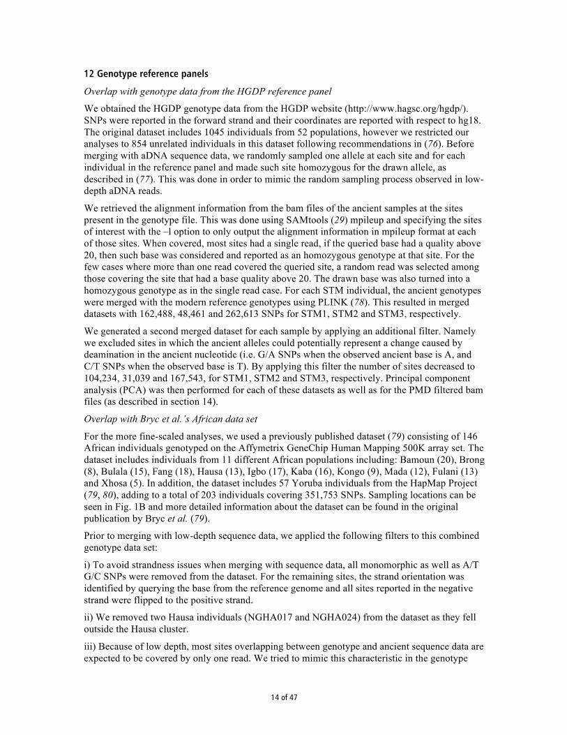
14 of 47

12 Genotype reference panels

Overlap with genotype data from the HGDP reference panel

We obtained the HGDP genotype data from the HGDP website (http://www.hagsc.org/hgdp/). SNPs were reported in the forward strand and their coordinates are reported with respect to hg18. The original dataset includes 1045 individuals from 52 populations, however we restricted our analyses to 854 unrelated individuals in this dataset following recommendations in (76). Before merging with aDNA sequence data, we randomly sampled one allele at each site and for each individual in the reference panel and made such site homozygous for the drawn allele, as described in (77). This was done in order to mimic the random sampling process observed in low-depth aDNA reads.

We retrieved the alignment information from the bam files of the ancient samples at the sites present in the genotype file. This was done using SAMtools (29) mpileup and specifying the sites of interest with the –l option to only output the alignment information in mpileup format at each of those sites. When covered, most sites had a single read, if the queried base had a quality above 20, then such base was considered and reported as an homozygous genotype at that site. For the few cases where more than one read covered the queried site, a random read was selected among those covering the site that had a base quality above 20. The drawn base was also turned into a homozygous genotype as in the single read case. For each STM individual, the ancient genotypes were merged with the modern reference genotypes using PLINK (78). This resulted in merged datasets with 162,488, 48,461 and 262,613 SNPs for STM1, STM2 and STM3, respectively.

We generated a second merged dataset for each sample by applying an additional filter. Namely we excluded sites in which the ancient alleles could potentially represent a change caused by deamination in the ancient nucleotide (i.e. G/A SNPs when the observed ancient base is A, and C/T SNPs when the observed base is T). By applying this filter the number of sites decreased to 104,234, 31,039 and 167,543, for STM1, STM2 and STM3, respectively. Principal component analysis (PCA) was then performed for each of these datasets as well as for the PMD filtered bam files (as described in section 14).

Overlap with Bryc et al.’s African data set

For the more fine-scaled analyses, we used a previously published dataset (79) consisting of 146 African individuals genotyped on the Affymetrix GeneChip Human Mapping 500K array set. The dataset includes individuals from 11 different African populations including: Bamoun (20), Brong (8), Bulala (15), Fang (18), Hausa (13), Igbo (17), Kaba (16), Kongo (9), Mada (12), Fulani (13) and Xhosa (5). In addition, the dataset includes 57 Yoruba individuals from the HapMap Project (79, 80), adding to a total of 203 individuals covering 351,753 SNPs. Sampling locations can be seen in Fig. 1B and more detailed information about the dataset can be found in the original publication by Bryc et al. (79).

Prior to merging with low-depth sequence data, we applied the following filters to this combined genotype data set:

i) To avoid strandness issues when merging with sequence data, all monomorphic as well as A/T G/C SNPs were removed from the dataset. For the remaining sites, the strand orientation was identified by querying the base from the reference genome and all sites reported in the negative strand were flipped to the positive strand.

ii) We removed two Hausa individuals (NGHA017 and NGHA024) from the dataset as they fell outside the Hausa cluster.

iii) Because of low depth, most sites overlapping between genotype and ancient sequence data are expected to be covered by only one read. We tried to mimic this characteristic in the genotype

15 of 47

dataset by randomly sampling one allele at each site and for each individual and making the site homozygous for the drawn allele, as done in (77).

After filtering we retained 294,651 sites in 201 individuals. The filtered genotype data was then merged with the low-depth sequence data, as described above for the HDGP dataset. The merged data sets consisted of 73,926, 21,819, and 119,140 SNPs for STM1, STM2 and STM3, respectively.

13 D-statistic tests

We used D-statistics as previously described (82) to determine the relationship between the Zoutsteeg Three and a set of 11 previously published high coverage genomes from different worldwide populations (17). For each of the Zoutsteeg Three, we calculated D-statistics of the form:

D(chimp, STM; Yoruba, X)

with X representing all modern human genomes other than Yoruba. The expected value for this configuration is D=0 if Yoruba and population X are equally closely related to the one of the Zoutsteeg Three (STM). If the Zoutsteeg individual is more closely related to Yoruba, the statistic is expected to be negative, while it will be positive if individual X is more closely related. By analyzing all configurations with the modern individuals X in turn, we are therefore testing whether the Zoutsteeg individuals are more closely related to any modern individuals than to Yoruba. The significance of the deviation from D=0 was assessed by calculating a Z-score from a block jackknife as previously described (82), using a block size of 5 MB.

We applied this test to each of the STMs, with results shown in Fig. S16 (D-statistics and Z-scores are listed in Table S6). We find that each STM individual is significantly closer related to Yoruba than to any non-African individual, consistent with an African origin of the individuals. Within Africa, the ancient individuals are significantly closer related to Yoruba than to individuals from hunter-gatherer populations (San, Mbuti Pygmy). The only non-significant statistics result from tests involving Mandenka and Dinka. This is more likely to be due to a lack of ancient sequence data, as opposed to low population differentiation (Fst) between these populations.

14 Principal component analysis

For each file containing the genotypes of the sample and reference panels, we ran smartpca (EIGENSOFT vers. 4.0) (83, 84) to perform principal components analysis (PCA). We also ran smartpca on the filtered reference panel (prior to step iii. in section 12) to calculate the reference-only eigenvectors. Eigenvectors were plotted independently for each dataset using RStudio (http://www.rstudio.org/). In order to visualize the three samples in a single PCA plot we used the VEGAN package (http://vegan.r-forge.r-project.org) to perform Procrustes transformation in R, as done in (77). We transformed the first two principal components calculated for each intersected dataset to match the reference-only PC1 and PC2. When transforming the PCs, the ancient individual was excluded. The configuration of transformed PC1 and PC2 was then applied to the ancient individuals, and transformed coordinates were overlaid on the reference-only PC1 and PC2 plot (Fig. 1C). Individual PCA plots for STM1-3 are shown in Fig. S19.

Assessing the effect of potential contamination

We used PMDtools (31) to filter bam files and retain only reads carrying the characteristic signatures of aDNA damage. We selected reads with a pmd (post-mortem damage) score of ≥3 (retaining 58,078, 59,994 and 103,464 reads after setting the pmd threshold of 3 for STM1, STM2, STM3, respectively) and intersected them with the reference panel to assess if the PCA

16 of 47

using only damaged reads displayed the same clustering of the sample as with the unfiltered set (Fig. S18).

15 TreeMix analysis

We used the files with the intersected genotypes between our samples and our reference panel (79) to estimate the allele frequencies per population and considering each of the Zoutsteeg individuals as one population, therefore the allele frequency would always be either 0 or 1 (or 0 and 2 in terms of allele counts). We used PLINK (78) to estimate allele frequencies per population and formatted the output with the script plink2treemix.py distributed along with the TreeMix (85) software. We used these frequencies as input for TreeMix (85) in order to infer ancestry graphs. For each dataset we ran 100 bootstraps with random seeds and with the –noss and –global flags to disable sample size correction, and perform a round of global rearrangements of the graph, respectively. Additionally, the number of SNPs per block was calculated for each dataset to allow approximately 1000 blocks. Finally, the root of the tree was set to Xhosa. The results of the TreeMix (85) analysis are shown in Fig. S20.

16 Admixture analysis

We used the maximum likelihood-based clustering algorithm ADMIXTURE (86) to estimate the genetic structure in our merged dataset (see section 12). We first estimated the cross-validation error running ADMIXTURE (86) with the --cv flag for K values between 1 and 6. This analysis revealed that the CV error increased with K, probably reflecting the very low Fst between the populations in such reference panel. For K=4 to K=6 we ran a hundred replicates using a random seed and kept the Q (ancestral cluster proportions) and P (inferred ancestral cluster allele frequencies) matrices from the run with the best log likelihood. We used the P matrix from each K to estimate the most likely cluster proportions in the ancient samples as was done in (87). Fig. S21 shows the ancestry proportions of STM1, STM2 and STM3 and 11 sub-Saharan populations from our reference panel (79). Plots were generated using a maximum-likelihood approach implemented in ADMIXTURE (86) and show converged runs from K=2 to K=6 in 100 replicates.

17 of 47

Supplementary Figures

Fig. S1. Late 17th-century artifacts found in the same layer as three Zoutsteeg burials. Reproduced with permission from ref. 11.

18 of 47

Fig. S2. STM1 maxilla showing a type of dental modification common in West-Central Africa. Reproduced with permission from ref. 11.

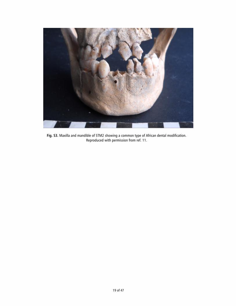
19 of 47

Fig. S3. Maxilla and mandible of STM2 showing a common type of African dental modification. Reproduced with permission from ref. 11.

20 of 47

Fig. S4. Maxilla of STM3 showing a modified incisor. Reproduced with permission from ref. 11.

21 of 47

Fig. S5. The calibrated radiocarbon dates obtained for the three individuals (STM1-3, 68% and 95% probability ranges given beneath). These results were added to a Bayesian model that also included the foundation date of St Martin (1735 AD), and an approximation for the turnover rate of bone collagen (10 ± 5 years). The modeled output for the date of the burials is given by the dark blue distribution [1667-1682 AD (68%); 1658-1691 AD (95%)]. The output if the assumption is made that the burials all took place in the same year is also given [light blue distribution, 1668-1681 AD (68%); 1660-1688 AD (95%)].

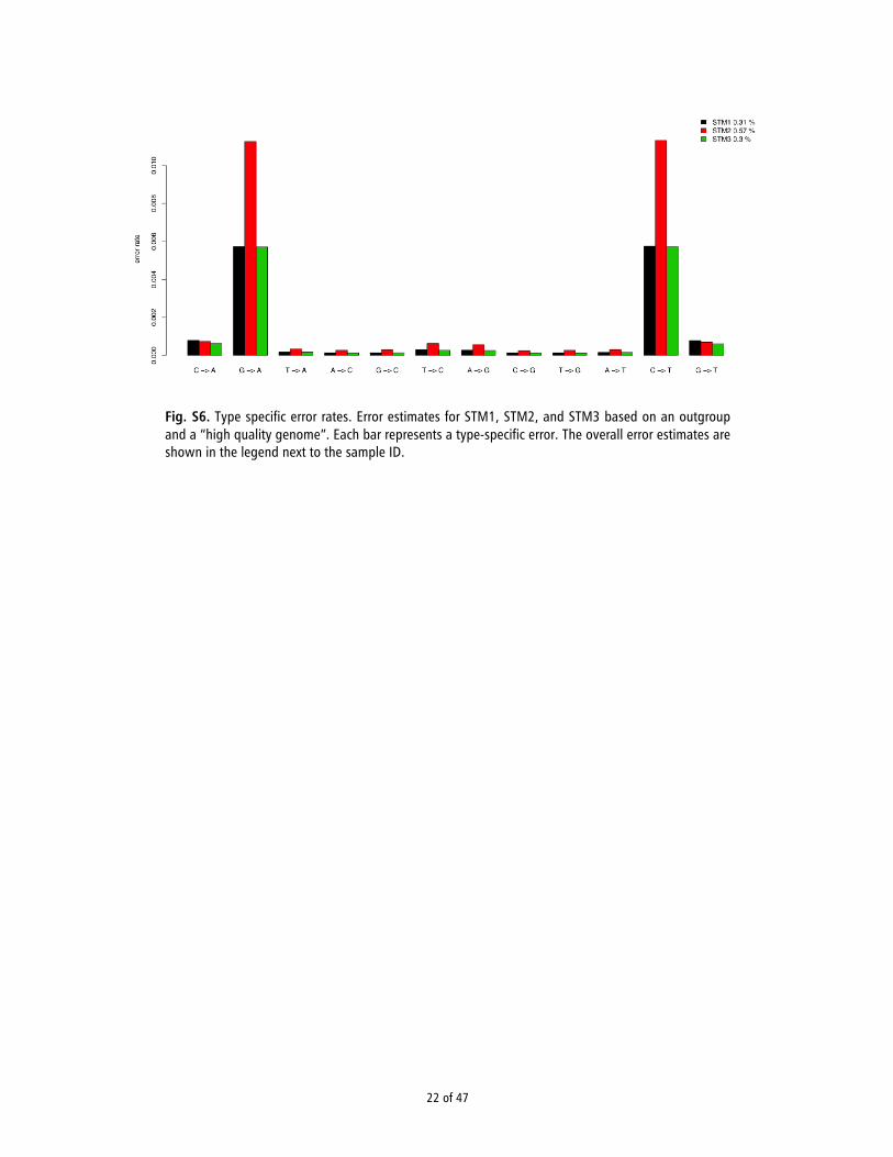
22 of 47

Fig. S6. Type specific error rates. Error estimates for STM1, STM2, and STM3 based on an outgroup and a “high quality genome”. Each bar represents a type-specific error. The overall error estimates are shown in the legend next to the sample ID.

23 of 47

Fig. S7. Damage patterns for STM1-3. Plots on the left show damage patterns for libraries built with the double-stranded method. Plots on the right show the patterns for those built with the single-stranded method. Plots were made with mapDamage2.0 (29).

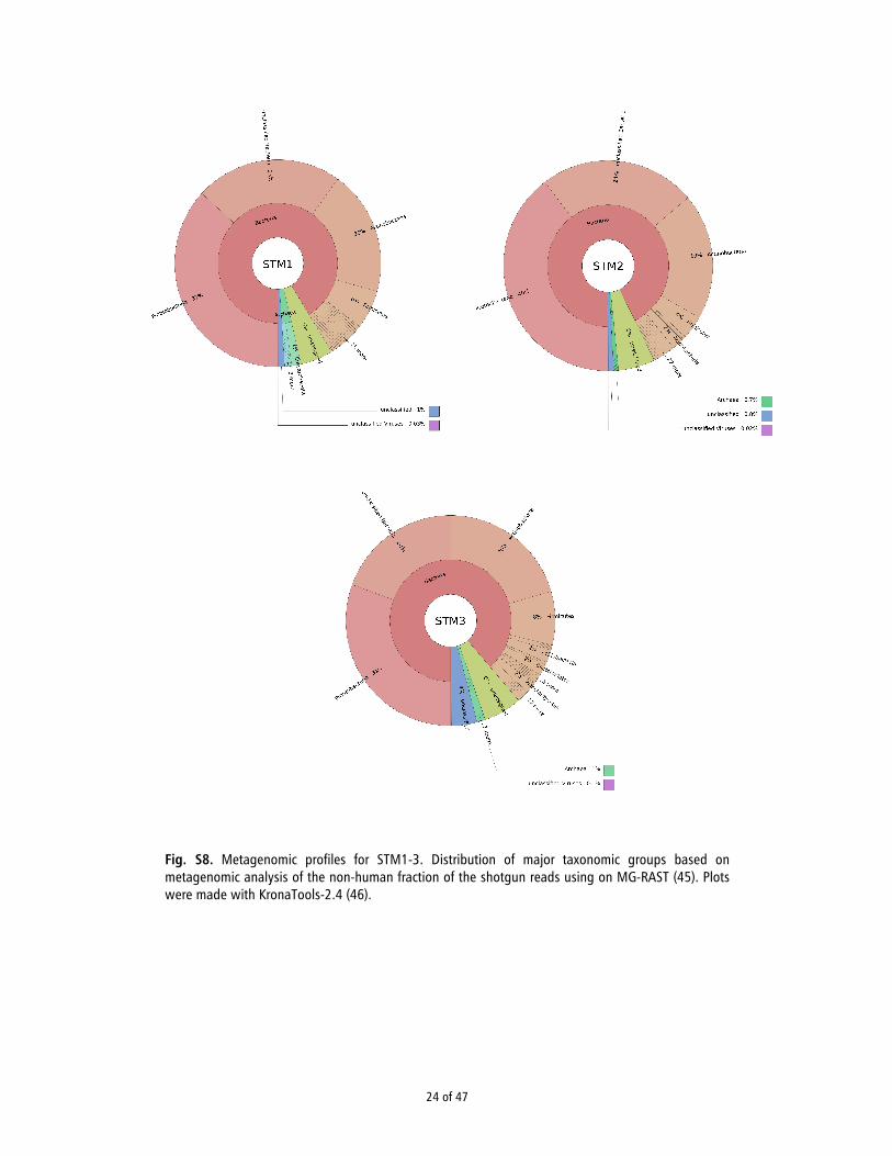
24 of 47

Fig. S8. Metagenomic profiles for STM1-3. Distribution of major taxonomic groups based on metagenomic analysis of the non-human fraction of the shotgun reads using on MG-RAST (45). Plots were made with KronaTools-2.4 (46).

25 of 47

Fig. S9. Read length distributions for samples STM1-3.

26 of 47

Fig. S10. Molecular decay rates for STM2. Nuclear and mitochondrial read length distributions showing only the declining part of the distributions, used to estimate DNA decay rates. Trendline, equation and R2 value represent best fit for an exponential decline, as expected under a model of random fragmentation. The correlation for mtDNA is weaker due to a smaller dataset and hence more stochasticity.

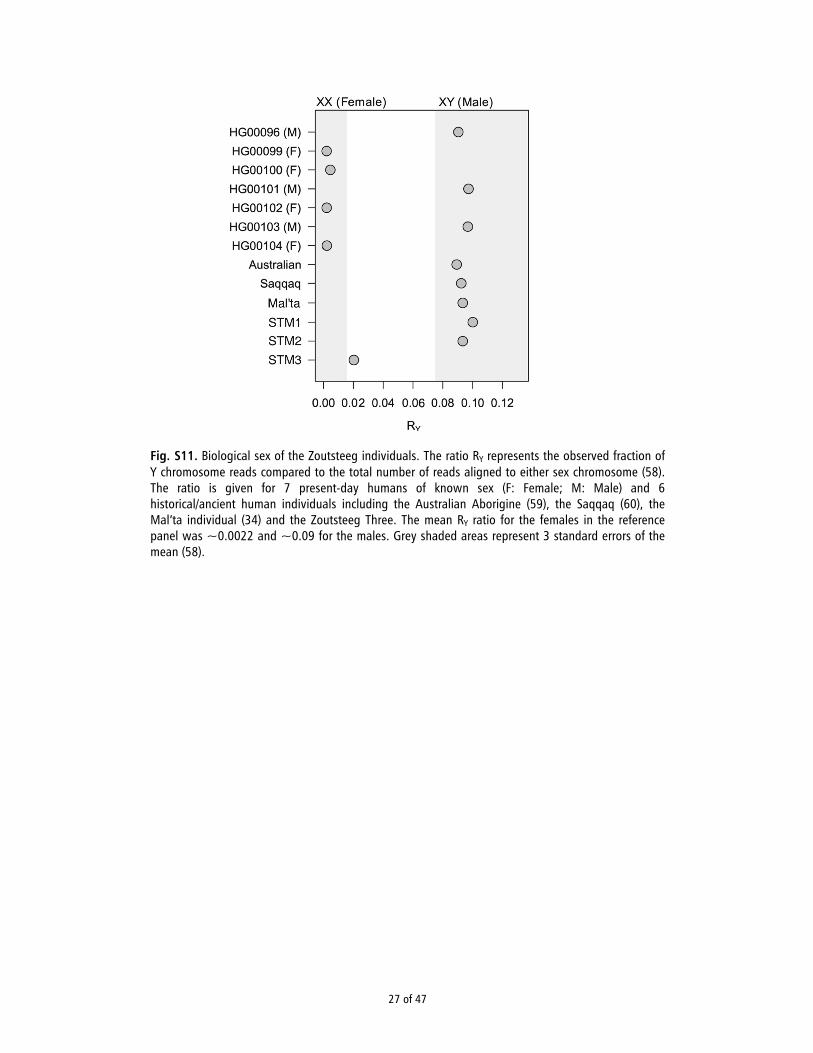
27 of 47

Fig. S11. Biological sex of the Zoutsteeg individuals. The ratio RY represents the observed fraction of Y chromosome reads compared to the total number of reads aligned to either sex chromosome (58). The ratio is given for 7 present-day humans of known sex (F: Female; M: Male) and 6 historical/ancient human individuals including the Australian Aborigine (59), the Saqqaq (60), the Mal’ta individual (34) and the Zoutsteeg Three. The mean RY ratio for the females in the reference panel was ~0.0022 and ~0.09 for the males. Grey shaded areas represent 3 standard errors of the mean (58).

28 of 47

Fig. S12. Maximum parsimony tree of the mitogenomes analyzed in the present study. The position of the rCRS (54) is indicated for reading off sequence motifs. Rectangular boxes contain haplogroup labels following Phylotree Build 16 (http://www.phylotree.org; and the rCRS orientated version). Mutational changes are shown along branches. In blue are polymorphisms falling in the control region. Mutations are transitions unless a suffix A, C, G, or T indicates a transversion. Other suffixes are: insertions (+), synonymous substitutions (s), mutations changes occurring at tRNAs (-t), mutational changes occurring at rRNAs (-r), non-coding variants located in the mtDNA coding region (-nc), and amino acid replacements. A back mutation is represented with the prefix “@”, whereas an underlined mutation represents a recurrent mutation in the phylogeny represented in the figure. As usual, variants at positions A16182C, A16183C, variation around position 310 and length or point heteroplasmies were not considered for the phylogenetic reconstruction.

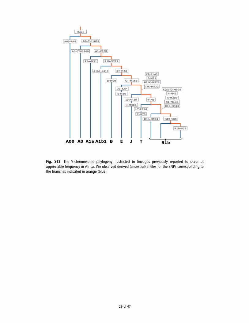
29 of 47

Fig. S13. The Y-chromosome phylogeny, restricted to lineages previously reported to occur at appreciable frequency in Africa. We observed derived (ancestral) alleles for the SNPs corresponding to the branches indicated in orange (blue).

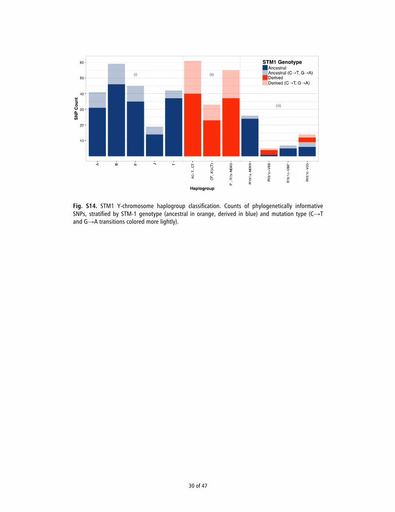
30 of 47

Fig. S14. STM1 Y-chromosome haplogroup classification. Counts of phylogenetically informative SNPs, stratified by STM-1 genotype (ancestral in orange, derived in blue) and mutation type (C→T and G→A transitions colored more lightly).

31 of 47

Fig. S15. The Y-chromosome lineage of STM1, with respect to 29 low-coverage R1b1c-V88 sequences from (65) and two higher coverage R1b1a-M269 sequences from (36). Divergence times indicated in grey were directly estimated, and their difference was used to infer an 8.5 kya split-time between STM1 and the Sardinian V35 lineages. The shortness of the STM1 branch is due to low coverage.

(11)

R1b1a-S116

STM-1

(18)

R1b1a-Z2105

R1b-M343

R1b1c-V35

R1b1a-M269

R1b1c-V88*

R1b1c-V885

1

2

3

4

7

6

~ 23.0 ky

~ 14.5 ky ~ 8.5 ky

32 of 47

Fig. S16. Results for sequence-based D-statistic test. The test takes the form D(chimp, STM; Yoruba, X) with STM standing for one of the Zoutsteeg Three and X representing one of 11 modern human genomes other than Yoruba (17). We find that each of the Zoutsteeg individuals is significantly closer related to Yoruba than to any non-African individual, consistent with an African origin of the individuals. Within Africa, the ancient individuals are significantly closer related to Yoruba than to individuals from hunter-gatherer populations (San, Mbuti pygmies). The only non-significant statistics result from tests involving Mandenka and Dinka, which are consistent with forming a clade with Yoruba to the exclusion of the ancient individuals. This is likely a consequence of a lack of power to detect more fine scale population relatedness within sub-Saharan African populations that are not of a hunter-gatherer origin. D-statistic values and Z scores are listed in Table S6.

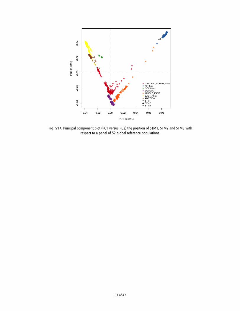
33 of 47

Fig. S17. Principal component plot (PC1 versus PC2) the position of STM1, STM2 and STM3 with respect to a panel of 52 global reference populations.

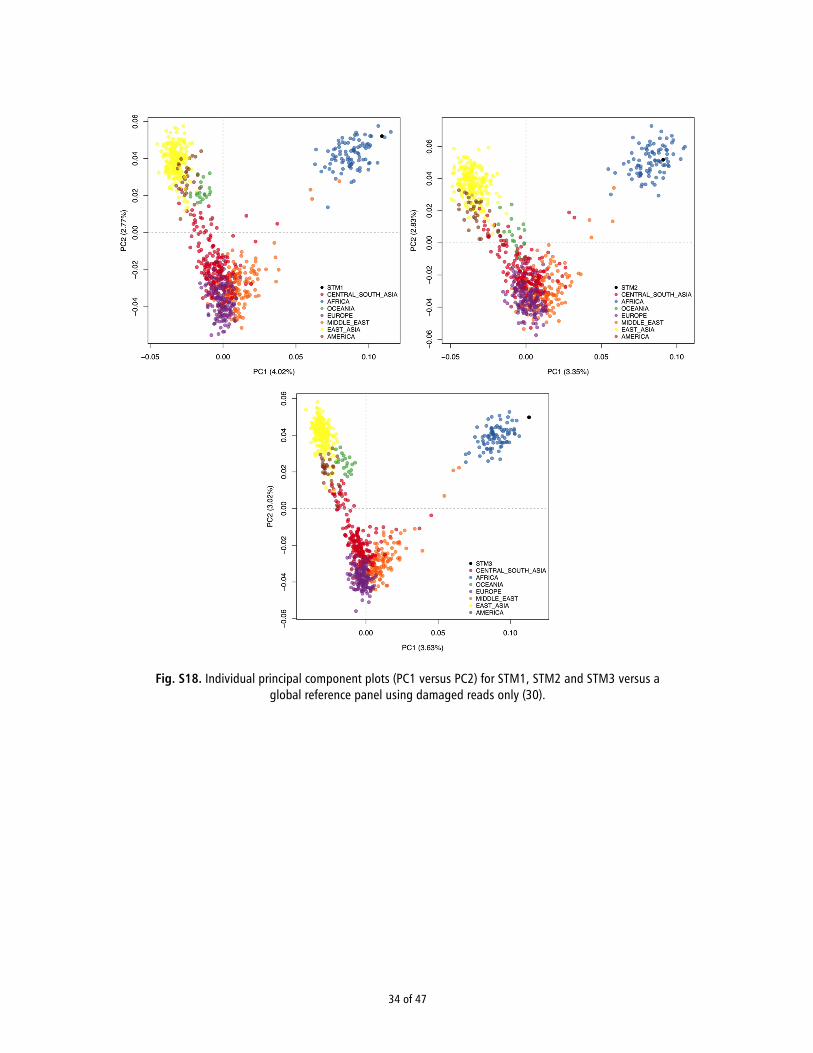
34 of 47

Fig. S18. Individual principal component plots (PC1 versus PC2) for STM1, STM2 and STM3 versus a global reference panel using damaged reads only (30).

35 of 47

Fig. S19. Individual principal component plots (PC1 versus PC2) for STM1, STM2 and STM3 and 11 African populations from our reference panel (78). Plots have been rotated to mirror the geographic distribution of the reference populations.

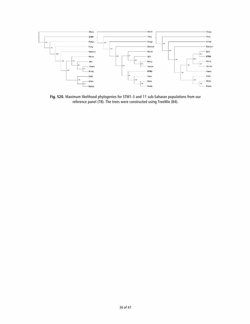
36 of 47

Fig. S20. Maximum likelihood phylogenies for STM1-3 and 11 sub-Saharan populations from our reference panel (78). The trees were constructed using TreeMix (84).

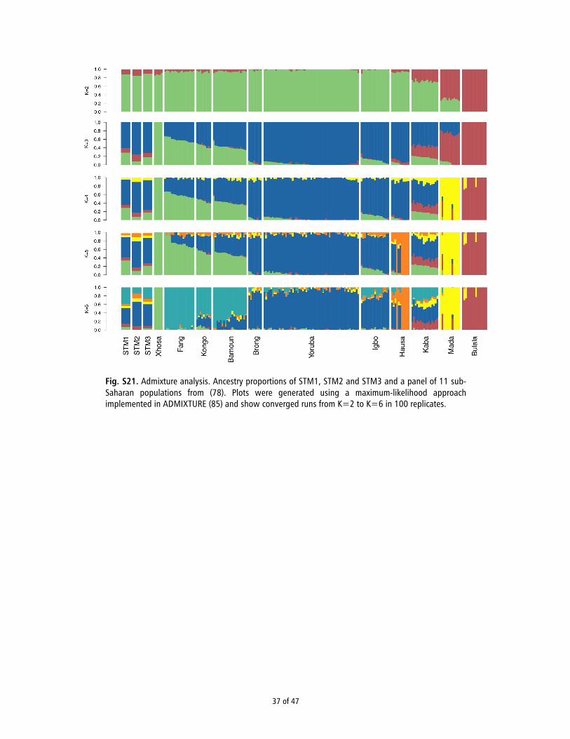
37 of 47

Fig. S21. Admixture analysis. Ancestry proportions of STM1, STM2 and STM3 and a panel of 11 sub-Saharan populations from (78). Plots were generated using a maximum-likelihood approach implemented in ADMIXTURE (85) and show converged runs from K=2 to K=6 in 100 replicates.

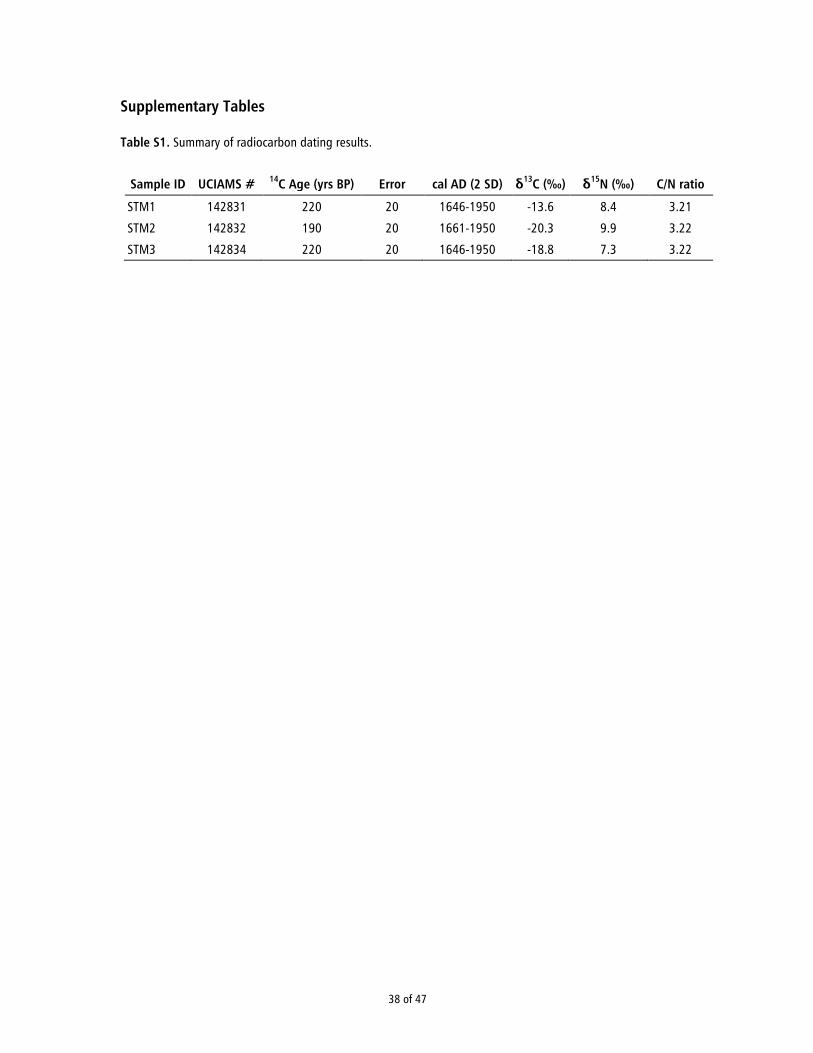
38 of 47

Supplementary Tables Table S1. Summary of radiocarbon dating results.

Sample ID UCIAMS # 14C Age (yrs BP) Error cal AD (2 SD) δ13C (‰) δ15N (‰) C/N ratio

STM1 142831 220 20 1646-1950 -13.6 8.4 3.21

STM2 142832 190 20 1661-1950 -20.3 9.9 3.22

STM3 142834 220 20 1646-1950 -18.8 7.3 3.22

39 of 47

Table S2. Sequencing results for double-stranded libraries before and after whole genome capture.

Before capture (shotgun) After capture (WISC/MYBait)

STM1 STM2 STM3 STM1 STM2 STM3

Raw reads 122,654,644 377,671,782 111,370,579 85,135,530 395,550,610 75,195,196

Trimmed reads 115,192,135 350,113,051 99,196,939 83,337,755 383,644,976 72,023,222

Mapped reads 3,369,606 1,264,824 8,685,823 20,941,366 36,236,367 24,640,959

Unique reads 3,323,371 1,253,484 8,518,830 12,447,508 2,128,028 16,455,675

Endogenous (%) 2.7 0.3 7.6 14.6 0.5 21.9

Clonality (%) 1.4 0.9 1.9 40.6 94.1 33.2

Read length 80.5 69.9 81.1 88.3 86.1 87.6

40 of 47

Table S3. Sequencing results for single-stranded libraries before and after whole genome capture.

Before capture (shotgun) After capture (WISC/MYBait)

STM1 STM2 STM3 STM1 STM2 STM3

Raw reads 1,157,288 871,151 1,203,557 34,742,844 121,722,782 31,466,527

Trimmed reads 1,035,524 779,225 1,082,887 30,278,361 103,569,318 28,039,274

Mapped reads 55,371 13,618 175,600 6,059,526 12,006,896 10,157,948

Unique reads 55,290 13,595 175,302 2,331,771 1,484,184 7,219,555

Endogenous (%) 5.3 1.7 16.2 6.7 1.2 22.9

Clonality (%) 1.4 0.9 1.9 61.5 87.6 28.9

Read length 55.1 49.2 62.6 64.9 64.4 70.7

41 of 47

Table S4. Comparison of DNA decay in genomic data from bones of different preservation environments. Approximate ages and estimated burial temperatures are listed. Lambda (λ) is the DNA damage fraction (per site) estimated directly from the fragment length distributions and 1/λ is the estimate true average DNA fragment length in the bone. Lambda is converted to decay rate (k, per site per year) by dividing with sample age. Molecular half-lives for 100 bp fragments are calculated as in (47). La Braña results are based on data from (50) and Clovis results are based on data from (35).

Age Temp. λ k Fragment length Half-life

STM2, Caribbean, nuDNA 340 yrs BP 25°C 0.014 4.12E-05 71 bp 169 yrs

STM2, Caribbean, mtDNA 340 yrs BP 25°C 0.012 3.53E-05 83 bp 197 yrs

La Braña, Spain, nuDNA 7,500 yrs BP 8°C 0.033 4.40E-06 30 bp 1,576 yrs

Anzick, Montana, nuDNA 12,800 yrs BP 5°C 0.018 1.41E-06 56 bp 4,916 yrs

42 of 47

Table S5. Contamination rate estimates for each sample. The second column represents the number of reads for each sample mapping to the consensus mtDNA sequence. The point estimate error rate is shown on the third column. The maximum a posteriori probability and 95% credible interval for the contamination rate are on column four and five, respectively. Mt reads Error rate MAP contamination (%) 95% CI

STM1 50,868 0.011 0.63 0.32-1.07

STM2 49,784 0.012 0.22 0.02-0.63

STM3 51,441 0.008 0.15 0.03-0.38

43 of 47

Table S6. Summary results for sequence data-based D-statistic tests. H1 stands for Yoruba, H2 for one of 10 other global populations (one genome per population) and H3 one of the STMs. The ‘Difference’ column shows the number of ABBA minus the number of BABA sites (nABBA-nBABA); the ‘Total’ column shows the total number of ABBA and BABA sites (nABBA+nBABA); the ‘Dstat’ column lists the test statistic (nABBA-nBABA)/(nABBA+ nBABA); the ‘Jackknife’ column shows the bias corrected Dstat; the ‘SE’ column shows the estimated standard error of the estimate used to obtain the Z value; and, the ‘Z’ column shows the significance value of the test. Negative D-statistics correspond to H3 sharing more alleles with Yoruba than with H2.

H1 H2 H3 Difference Total Dstat Jackknife SE Z

Yoruba San STM1 -52,331 350,007 -0.149514 -0.149514 0.004348 -34.38317

Yoruba Mbuti STM1 32,882 342,222 -0.096084 0.096084 0.004449 -21.59600

Yoruba Mandenka STM1 -3,374 330,114 -0.010221 -0.010221 0.004460 -2.29165

Yoruba Dinka STM1 1,629 329,483 -0.004944 0.004944 0.004136 -1.19550

Yoruba Sardinian STM1 9,442 331,046 -0.028522 0.028522 0.004437 -6.42871

Yoruba French STM1 10,030 332,086 -0.030203 0.030203 0.004328 -6.97929

Yoruba Han STM1 11,093 332,789 -0.033333 0.033333 0.004225 -7.88885

Yoruba Dai STM1 -10,330 331,586 -0.031153 -0.031153 0.004269 -7.29738

Yoruba Karitiana STM1 -10,762 331,772 -0.032438 -0.032438 0.004602 -7.04889

Yoruba Papuan STM1 14,422 335,270 -0.043016 0.043016 0.004468 -9.62833

Yoruba San STM2 -18,983 122,475 -0.154995 -0.154995 0.004924 -31.47631

Yoruba Mbuti STM2 12,860 119,446 -0.107664 0.107664 0.004728 -22.77179

Yoruba Mandenka STM2 -1,413 115,559 -0.012228 -0.012228 0.004939 -2.47575

Yoruba Dinka STM2 1,393 115,375 -0.012074 0.012074 0.004835 -2.49731

Yoruba Sardinian STM2 3,165 116,101 -0.027261 0.027261 0.004865 -5.60317

Yoruba French STM2 3,034 116,092 -0.026134 0.026134 0.004721 -5.53532

Yoruba Han STM2 4,367 117,063 -0.037305 0.037305 0.004854 -7.68580

Yoruba Dai STM2 -3,000 116,536 -0.025743 -0.025743 0.004706 -5.47008

Yoruba Karitiana STM2 -4,206 116,780 -0.036016 -0.036016 0.005054 -7.12577

Yoruba Papuan STM2 4,839 117,977 -0.041016 0.041016 0.004987 -8.22500

Yoruba San STM3 -83,211 537,697 -0.154754 -0.154754 0.003817 -40.54369

Yoruba Mbuti STM3 53,652 526,988 -0.101809 0.101809 0.004104 -24.81020

Yoruba Mandenka STM3 -3,409 509,017 -0.006697 -0.006697 0.004099 -1.63399

Yoruba Dinka STM3 2,476 507,590 -0.004878 0.004878 0.004095 -1.19114

Yoruba French STM3 17,724 509,850 -0.034763 0.034763 0.004252 -8.17586

Yoruba Sardinian STM3 17,981 509,315 -0.035304 0.035304 0.004315 -8.18268

Yoruba Han STM3 19,042 513,304 -0.037097 0.037097 0.004303 -8.62139

Yoruba Dai STM3 -17,945 510,107 -0.035179 -0.035179 0.004187 -8.40273

Yoruba Karitiana STM3 -22,270 511,022 -0.043579 -0.043579 0.004165 -10.46407

Yoruba Papuan STM3 25,217 516,839 -0.048791 0.048791 0.004662 -10.46557

44 of 47

References

1. Nichols E (1989) The Last Miles of the Way: African-American Homegoing Traditions 1890-Present. South Carolina State Museum, Columbia, SC.

2. Jamieson RW (1995) Material Culture and Social Death: African-American Burial Practices. Hist Arch 29:39-58.

3. Bass WM (1987) Human osteology: a laboratory and field manual. Missouri Archaeological Society Inc., Columbia, MO.

4. Buikstra JE, Ubelaker DH (1994) Standards for Data Collection from Human Skeletal Remains. Arkansas Archaeological Survey, Fayetteville, AR.

5. von Jehring H (1882) Die künstliche Deformierung der Zähne. Zeitschrift für Ethnologie 14:213-62. 6. Lignitz H (1919-1922) Die künstlichen Zahnverstümmelungen in Afrika im Lichte der

Kulturkreisforschung. Anthropos 14-15:891-943. 7. Goose DH (1963) Tooth-mutilation in West Africans. Man 63:91-3. 8. Gould AR et al. (1984) Mutilations of the Dentition in Africa: A Review with Personal Observations.

Quintessence International 15:89-94. 9. Reichart PA et al. (2007) Dental mutilations and associated alveolar bone pathology in African

skulls of the anthropological skull collection, Charité, Berlin. J Oral Path Med 37:50-5. 10. Witkin A (2011) The human skeletal remains. In: A. Pearson et al. (eds.), Infernal Traffic: Excavation

of a Liberated African Graveyard in Rupert’s Valley, St Helena. CBA Research Report 169. Council for British Archeology, York, UK.

11. Schroeder H et al. (2014) The Zoutsteeg Three: Three New Cases of African Types of Dental Modification from Saint Martin, Dutch Caribbean. Int J Osteoarch 24:688-96.

12. Schroeder H et al. (2009) Trans-atlantic slavery: Isotopic evidence for forced migration to Barbados. Am J Phys Anth 139:547-57.

13. Price TD et al. (2006) Early African diaspora in colonial Campeche, Mexico: Strontium isotopic evidence. Am J Phys Anth 130:485-90.

14. Reimer PJ et al. (2013) IntCal13 and Marine13 Radiocarbon Age Calibration Curves 0–50,000 Years cal BP. Radiocarbon 55:1869-87.

15. The Transatlantic Slave Trade Database (available at http://slavevoyages.org). 16. Brown TA et al. (1988) Improved collagen extraction by modified Longin method. Radiocarbon

30:171-7. 17. Bronk Ramsey C (1995) Radiocarbon calibration and analysis of stratigraphy: the OxCal program.

Radiocarbon 37:425-30. 18. Bronk Ramsey C (2009), Bayesian analysis of radiocarbon dates. Radiocarbon 51:337-60. 19. Hedges REM et al. (2007) Collagen turnover in the adult femoral mid-shaft: modeled from

anthropogenic radiocarbon tracer measurements. Am J Phys Anth 133:808-16. 20. Wild EM et al. (2000) 14C dating with the bomb peak: an application to forensic medicine. Nucl

Instr Meth Phys Res B 172:944-50. 21. Rohland N, Hofreiter M (2007) Ancient DNA extraction from bones and teeth. Nature Protocols

2:1756-62. 22. Meyer M, Kircher M (2010) Illumina Sequencing Library Preparation for Highly Multiplexed Target

Capture and Sequencing. Cold Spring Harb Protoc 2010 (6), pdb.prot5448. 23. Gansauge MT, Meyer M (2013) Single-stranded DNA library preparation for the sequencing of

ancient or damaged DNA. Nature Protocols 8:737-48.

45 of 47

24. Carpenter ML et al. (2013) Pulling out the 1%: Whole-Genome Capture for the Targeted Enrichment of Ancient DNA Sequencing Libraries. Am J Hum Genet 93:852-64.

25. MYbaits manual (available at http://www.mycroarray.com/pdf/MYbaits-manual.pdf). 26. Ávila-Arcos MC et al. (in press) Comparative Performance of Two Whole Genome Capture

Methodologies on Ancient DNA Illumina Libraries. Methods Ecol Evol. DOI: 10.1111/2041-210X.12353

27. Lindgreen S (2012) AdapterRemoval: Easy Cleaning of Next Generation Sequencing Reads. BMC Res Notes 5:337.

28. Li H, Durbin R (2009) Fast and accurate short read alignment with Burrows-Wheeler transform. Bioinform 25:1754-60.

29. Li H et al. (2009) The Sequence Alignment/Map format and SAMtools. Bioinform 25:2078-9. 30. Jónsson H et al. (2013) mapDamage2.0: fast approximate Bayesian estimates of ancient DNA

damage parameters. Bioinform 29:1682-4. 31. Skoglund P et al. (2014) Separating endogenous ancient DNA from modern day contamination in a

Siberian Neandertal. Proc Natl Acad Sci USA 111:2229-34. 32. Reich D. et al. (2011) Genetic history of an archaic hominin group from Denisova Cave in Siberia.

Nature 468:1053-60. 33. Orlando L et al. (2013) Recalibrating Equus evolution using the genome sequence of an early

Middle Pleistocene horse. Nature 499:74-78. 34. The 1000 Genomes Project Consortium (2012) An integrated map of genetic variation from 1,092

human genomes. Nature 491:56-65. 35. Raghavan M et al. (2014) Upper Palaeolithic Siberian genome reveals dual ancestry of Native

Americans. Nature 505:87-91. 36. Rasmussen M et al. (2014) The genome of a Late Pleistocene human from a Clovis burial site in

western Montana. Nature 506:225-9. 37. Underhill PA et al. (2014) The phylogenetic and geographic structure of Y-chromosome haplogroup

R1a. Eur J Hum Genet 1-8. 38. Poznik GD et al. (2013) Sequencing Y chromosomes resolves discrepancy in time to common

ancestor of males versus females. Science 341:562-5. 39. Karolchik D et al. (2004) The UCSC Table Browser data retrieval tool. Nucleic Acids Res 32, D493-6. 40. NCBI: National Center for Biotechnology Information (available at http://www.ncbi.nlm.nih.gov) 41. Quinlan AR, Hall IM (2010) BEDTools: a flexible suite of utilities for comparing genomic features.

Bioinform 26:841-2. 42. Francalacci P et al. (2013) Low-pass DNA sequencing of 1200 Sardinians reconstructs European Y-

chromosome phylogeny. Science 341:P565-9. 43. Briggs AW et al. (2007) Patterns of damage in genomic DNA sequences from a Neandertal. Proc

Natl Acad Sci USA 104:14616-21. 44. Meyer M et al. (2012) A high-coverage genome sequence from an archaic Denisovan individual.

Science 338:222-6. 45. Campos PF et al. (2012) DNA in ancient bone – Where is it located and how should we extract it?

Ann Anat 194:7-16. 46. Meyer F et al. (2008) The Metagenomics RAST server – A public resource for the automatic

phylogenetic and functional analysis of metagenomes. BMC Bioinform 9:386. 47. Ondov BD et al., Interactive metagenomic visualization in a Web browser. BMC Bioinformatics 12,

385 (2011). 48. Allentoft ME et al. (2012) The half-life of DNA in bone: measuring decay kinetics in 158 dated

46 of 47

fossils. Proc R Soc B 279:4724-33. 49. Dabney J et al. (2013) Complete mitochondrial genome sequence of a Middle Pleistocene cave

bear reconstructed from ultrashort DNA fragments. Proc Natl Acad Sci USA 110:15758-63. 50. Deagle BE et al. (2006) Quantification of damage in DNA recovered from highly degraded

samples—a case study on DNA in faeces. Front Zool 3:11. 51. Olalde I et al. (2014) Derived immune and ancestral pigmentation alleles in a 7,000-year-old

Mesolithic European. Nature 507:225-8. 52. Lindahl T (1993) Instability and decay of the primary structure of DNA. Nature 362:709-15. 53. Smith CI et al. (2003) The thermal history of human fossils and the likelihood of successful DNA

amplification. J Hum Evol 45:203-17. 54. Fu Q. et al. (2013) A Revised Timescale for Human Evolution Based on Ancient Mitochondrial

Genomes. Curr Biol 23:553-9. 55. Andrews RM et al. (1999) Reanalysis and revision of the Cambridge reference sequence for human

mitochondrial DNA. Nat Genet 23:147. 56. Milne I et al. (2013) Using Tablet for visual exploration of second-generation sequencing data.

Brief Bioinf 14:193-202. 57. Gelman A, Rubin DB (1992) Inference from Iterative Simulation Using Multiple Sequences. Statist

Sci 7:457-511. 58. Plummer M et al. (2006) CODA: Convergence Diagnosis and Output Analysis for MCMC. R News

6:7-11. 59. Skoglund P et al. (2013) Accurate sex identification of ancient human remains using DNA shotgun

sequencing. J Arch Sci 40:4477-82. 60. Rasmussen M et al. (2011) An Aboriginal Australian Genome Reveals Separate Human Dispersals

into Asia. Science 334:94-8. 61. Rasmussen M et al. (2010) Ancient human genome sequence of an extinct Palaeo-Eskimo. Nature

463:757-62. 62. Kloss-Brandstätter A et al. (2010) HaploGrep: a fast and reliable algorithm for automatic

classification of mitochondrial DNA haplogroups. Hum Mut 32:25-32. 63. Cerezo M et al. (2011) New Insights into the Lake Chad Basin Population Structure Revealed by

High-Throughput Genotyping of Mitochondrial DNA Coding SNPs. PLoS ONE 6:e18682. 64. Salas A et al. (2002) The making of the African mtDNA landscape. Am J Hum Genet 71:1082-111. 65. Beleza S et al. (2005) The genetic legacy of western Bantu migrations. Hum Genet 117:366-375. 66. Fendt L et al. (2012) MtDNA diversity of Ghana: a forensic and phylogeographic view. Forensic Sci

Int Genet 6:244-9. 67. Hünemeier T et al. (2007) Niger-Congo speaking populations and the formation of the Brazilian

gene pool: mtDNA and Y-chromosome data. Am J Phys Anth 133:854-67. 68. Jackson BA et al. (2005) Mitochondrial DNA genetic diversity among four ethnic groups in Sierra

Leone. Am J Phys Anth 128:156-63. 69. Plaza S et al. (2004) Insights into the western Bantu dispersal: mtDNA lineage analysis in Angola.

Hum Genet 115:439-47. 70. Rosa A et al. (2004) MtDNA Profile of West Africa Guineans: Towards a Better Understanding of

the Senegambia Region. Ann Hum Genet 68:340-52. 71. Soares P et al. (2012 )The Expansion of mtDNA Haplogroup L3 within and out of Africa. Mol Biol

Evol 29:915-27. 72. Salas A et al. (2004) The African diaspora: Mitochondrial DNA and the Atlantic slave trade. Am J

Hum Genet 74:454-65.

47 of 47

73. Salas A et al. (2005) Charting the ancestry of African Americans. Am J Hum Genet 77:676-80. 74. Ely B et al. (2006) African-American mitochondrial DNAs often match mtDNAs found in multiple

African ethnic groups. BMC Biol 4:34. 75. Cruciani F. et al. (2010) Human Y chromosome haplogroup R-V88: a paternal genetic record of

early mid Holocene trans-Saharan connections and the spread of Chadic languages. Eur J Hum Genet 18:800-7.

76. Rosenberg NA (2006) Standardized subsets of the HGDP-CEPH Human Genome Diversity Cell Line Panel, accounting for atypical and duplicated samples and pairs of close relatives. Ann Hum Genet 70:841-7.

77. Skoglund P et al. (2012) Origins and genetic legacy of Neolithic farmers and hunter-gatherers in Europe. Science 336:466-9.

78. Purcell S et al. (2007) PLINK: a tool set for whole-genome association and population-based linkage analyses. Am J Hum Genet 81:559-75.

79. Bryc K et al. (2010) Genome-wide patterns of population structure and admixture in West Africans and African Americans. Proc Natl Acad Sci USA 107:786-91.

80. The International HapMap Consortium (2007) A second generation human haplotype map of over 3.1 million SNPs. Nature 449:851-61.

81. The International HapMap 3 Consortium (2010) Integrating common and rare genetic variation in diverse human populations. Nature 467:52-8.

82. Durand EY et al. (2011) Testing for ancient admixture between closely related populations. Mol Biol Evol 28:2239-52.

83. Patterson N et al. (2006) Population structure and eigenanalysis. PLoS Genet 2:e190. 84. Price AL et al. (2006) Principal components analysis corrects for stratification in genome-wide

association studies. Nat Genet 38:904-9. 85. Pickrell JK, Pritchard JK (2012) Inference of Population Splits and Mixtures from Genome-Wide

Allele Frequency Data. PLoS Genet 8:e1002967. 86. Alexander DH et al. (2009) Fast model-based estimation of ancestry in unrelated individuals.

Genome Res 19:1655-64. 87. Sikora M et al. (2014) Population genomic analysis of ancient and modern genomes yields new

insights into the genetic ancestry of the Tyrolean Iceman and the genetic structure of Europe. PLoS Genet 10:e1004353.