NCAR/TN-367+STRNCAR TECHNICAL NOTE

January 1992

GENLN2A General Line-by-Line AtmosphericTransmittance and Radiance Model

Version 3.0 Description and Users Guide

D.P. Edwards

Atmospheric Chemistry Division

NATIONAL CENTER FOR ATMOSPHERIC RESEARCHBOULDER, COLORADO

· · I

i

CONTENTS

PageLIST OF FIGURES . . . . . . . . . . . . . . . . vLIST OF TABLES . . . . . . . . . . . . . . . . . . . . viiPREFACE . .. . .. ... .. . ..... .. .. .. .. .. ixACKNOWLEDGEMENTS ....................... xi

1. INTRODUCTION1.1 Atmospheric Radiative Transfer ..................... 11.2 The GENLN2 Suite of Programs .. . . . . . . . . . . .... . 21.3 Input File Formats for GENLN2 Input Files . . . . . . . . . . . . . . . 31.4 GENLN2 Implementation . . . . . . . . . . . . . . . 3

2. SPECTRAL LINE DATA: PROGRAM HITLIN2.1 Spectral Line Data Bases ....................... 72.2 Overview of Program HITLIN ..................... 72.3 Line Coupling . . . . . . . . . . . . . . . . . . . . . . . .. . 82.4 Description of HITLIN Subroutines. 82.5 Description of the HITLIN Input File .................. 92.6 HITLIN Implementation . . . . . . . . . . . . . . . . . . 10

3. ATMOSPHERIC MODELLING: PROGRAM LAYERS3.1 Layers, Paths, and Mixed Paths . ................... 153.2 Overview of Program LAYERS ... . . . . . . . . . . . . . . . . 153.3 Atmospheric Profiles ........................ 163.4 Atmospheric Layering ......................... 163.5 Description of LAYERS Subroutines . . . . . . . . . . . . . . . . . . . 183.6 Description of the LAYERS Input File ................. 193.7 LAYERS Implementation . . . .................... 22

4. THE LINE-BY-LINE CALCULATION: PROGRAM GENLN24.1 Overview of Program GENLN2 ................... . 314.2 Spectral Modelling . . . . . . . . . . . . . . . . . . . . . . . . . 314.3 Line Shape Modelling . . . . . . . . . . . . . . . . . . . . . . . . . 324.4 Molecular Cross-Section Data . . . . . . . . . . . . . . . . . . . . . 344.5 The Line-By-Line Calculation ............... .. . . 354.6 Continuum Absorption . . . . . . . . . . . . . . . . . . . . . 364.7 Transmittance Calculations ...................... 384.8 Radiance Calculations . . .. . . . . . . . . . . . .. . . . . . . . . 394.9 Description of GENLN2 Subroutines . . . . . . . . . . . . . . . . . 414.10 Description of the GENLN2 Input File ................. 444.11 GENLN2 Implementation . . . . . . . . . . . . . . . ........ 51

5. GRAPHICS AND POST-PROCESSING: PROGRAMS GENGRP AND RDOUT5.1 Overview of Program GENGRP . . . . . . . . . . . . . . . . . . . 635.2 Description of GENGRP Subroutines . . . . . . . . . . . . 635.3 Description of the GENGRP Interactive Input ... . . . . . . . . . . . 655.4 GENGRP Implementation ....................... 695.5 Overview of Program RDOUT . . . . . . . . . . . . . 69

iii

6. CALCULATIONS WITH A RADIOMETER: PROGRAMS BRIGHT AND RADTEM6.1 Overview of Programs BRIGHT and RADTEM . . . . . . . ... . . . .736.2 Description of BRIGHT and RADTEM Subroutines . . . . . . . . . . . . 746.3 Description of the BRIGHT Interactive Input . . . . . . . . . . 756.4 BRIGHT Implementation ...................... 756.5 Description of the RADTEM Interactive Input . . . . . . . . . . 766.6 RADTEM Implementation . . . . . . . . . . .. . . . . . . . . 77

APPENDIX 1. EXAMPLE CALCULATION 1: NADIR VIEWAl.l Overview of Example Calculation 1 ................. 81A1.2 Program HITLIN . .. . . . . . . 81A1.3 Program LAYERS ......................... 81A1.4 Program GENLN2 .............. ......... . 82A1.5 Program GENGRP ..................... 83A1.6 Programs RADTEM and BRIGHT ................. 83

APPENDIX 2. EXAMPLE CALCULATION 2: LIMB VIEWA2.1 Overview of Example Calculation 2 ........... ...... 107A2.2 Program HITLIN . ........................ 107A2.3 Program LAYERS ...... ................... 107A2.4 Program GENLN2 . ............ .......... 108A2.5 Program GENGRP ........................ 109

APPENDIX 3. EXAMPLE PMR CALCULATIONA3.1 Overview of Example PMR Calculation 1 . . . . ...... . 123A3.2 Modelling the PMR Response Functions .. ............. 123A3.3 The Gas Correlation Response Function ... 124A3.4 Example PMR Calculation: ISAMS CO2 Channel 7.1 . . . . . . ... 125A3.5 Program GENLN2: Calculation of the cell transmittances ....... 125A3.6 Program PMRFIL . ........................ 125A3.7 Program GENLN2: Atmospheric Calculation ............. 126A3.8 Program BRIGHT . .................... 127

REFERENCES .......... 144

iv

LIST OF FIGURES

1. INTRODUCTION1.1 Transmittance of radiation through a slab of absorbing material1.2 The GENLN2 suite of programs ...............

2. SPECTRAL LINE DATA: PROGRAM HITLIN2.1 Program structure for the HITLIN subroutines .

3. ATMOSPHERIC MODELLING: PROGRAM LAYERS3.1 Decomposition of an atmospheric path of mixed gases into layersand single gas paths . . . . . . . .. ..3.2 Geometry of a limb path through a refractive atmosphere ....3.3 Program structure for the LAYERS subroutines.

4. THE LINE-BY-LINE CALCULArION: PROGRAM GENLN24.1 The GENLN2 spectral calculation scheme ..........4.2 Uplooking radiance in a tropical atmosphere .........4.3 Illustration of mixed paths formed from the paths of Fig.3.1 anddefined by mixing table . . . . . . . . . . . . . . . ...4.4 Program structure for the GENLN2 subroutines

Page

. . . . . 5

. . . . 116

. . . . . 11

232425

... . . . 53

... . . . 54

. . . . . . 55... . . . 56

5. GRAPHICS AND POST-PROCESSING: PROGRAMS GENGRP AND RDOUT5.1 Program structure for the GENGRP subroutines . . . . . . . . . .. 70

6. CALCULATIONS WITH A RADIOMETER: PROGRAMS BRIGHT AND RADTEM6.1 Program structure for the BRIGHT and RADTEM subroutines ....... 78

APPENDIX 1. EXAMPLE CALCULATION 1: NADIR VIEWA1.1 Paths, mixed paths and radiating atmospheres for the nadir viewof Example Calculation 1 . . . . . . . . . . . . . . . . . . . . . . . .84

APPENDIX 2. EXAMPLE CALCULATION 2: LIMB VIEWA2.1 Paths, mixed paths and radiating atmospheres for the limb viewof Example Calculation 2 ...................... ..

APPENDIX 3. PMR CALCULATIONA3.1 ISAMS channel 7.1 response functions . . . . . . . . .....A3.2 Principle features of a pressure modulator radiometer (PMR) ......A3.3 Transmittance of a line in a PMR cell................

110

128129129

v

LIST OF TABLES

Page2. SPECTRAL LINE DATA: PROGRAM HITLIN

2.1 Gas molecular ID's .......................... 122.2 Format of the HITRAN line data base ............. . 132.3 Program HITLIN reference input file ................. 14

3. ATMOSPHERIC MODELLING: PROGRAM LAYERS3.1 Program LAYERS reference input file . . . . . .. . . . . . . . . . . . 263.2 Example of user profile data arrangement . . . . . . . . . . . . . . . .283.3 Listing of the PARRAY parameter file .... . . . . 29

4. THE LINE-BY-LINE CALCULATION: PROGRAM GENLN24.1 Program GENLN2 reference input file . . . . . . . . . . . . . . . . . . 584.2 Format of molecular cross-section data file . . . . . . . . . . . . . . . . 62

5. GRAPHICS AND POST-PROCESSING: PROGRAMS GENGRP AND RDOUT

5.1 Example of the External Spectra Data Arrangement . . . . . . . . 71

6. CALCULATIONS WITH A RADIOMETER: PROGRAMS BRIGHT AND RADTEM6.1 Example of radiance to brightness temperature look-up file . . . . . . . . . 79

vii

PREFACE

This report constitutes the latest documentation for Version 3.0 of the GENLN2 suiteof programs as of November 1991.

The need for a new atmospheric transmittance and radiance model at Oxford was rec-ognized by John Eyre of the UK Meteorological Office Unit in the Robert Hooke Institutefor Cooperative Atmospheric Research in 1986. At the time, more than 25 members of theDepartment of Atmospheric Physics and Hooke Institute at Oxford University were engagedin radiative transfer calculations or were direct users of such data. It was decided that therewas a strong case for developing a general purpose computation facility which would reducethe time spent duplicating effort in this area. Previously, a general line-by-line code GENLINhad been in use in Oxford. This along with other local codes was found to be limiting andinflexible, and although powerful facilities already existed, for example the Air Force Geo-physical Laboratory's FASCODE (Clough et al., 1988), a total re-design to meet current andanticipated needs was considered justified. This would hopefully promote understanding ofthe physical method and avoid the 'black-box' approach to computer modelling.

The essential computational model was designed first and coded afterwards. The mainaims were efficiency of calculation and a clear modular structure so that the model can beeasily adapted as a research tool for specific needs. This has taken precedence over speed ofcomputation or loosing sight of the physics in difficult to understand algorithms. The modelcan then be used in an educational role and enables workers to refine the treatment of onepart of the problem in isolation. Conversely, computations may also be performed quicklyand without the users having detailed knowledge of the calculation methods involved.

This report is intended to be a working document for those using GENLN2. A sep-arate section is devoted to each of the programs that comprise the GENLN2 suite. Eachsection begins with a brief overview of the purpose of the program and the physics involved.This is followed by a detailed description of the code structure, required input and codeimplementation. The appendices include the input and output for two example calculations.

Part of the work presented here was done during the time I held a post-doctoral positionin the Satellite Meteorology Group of the Hooke Institute in Oxford. The project has contin-ued since I moved to the Global Atmospheric Change Section of the Atmospheric ChemistryDivision at the National Center for Atmospheric Research, Boulder Co.

David P. EdwardsNovember 1991

Atmospheric Chemistry DivisionNational Center for Atmospheric ResearchP.O. Box 3000, Boulder, CO 80307-3C00Tel: (303) 497-1467, Fax: (303) 497-1492Email: edwards@ncar.ucar.edu

ix

ACKNOWLEDGEMENTS

I would like to acknowledge the initial guidance of this project by John Aire (ECM-RWF), Roger Saunders (U.K. Met. Office), and John Barnett (Oxford University) and thehelp of Peter Rayer (U.K. Met. Office). I am also grateful to Tony Clough (Atmosphericand Environmental Research Inc.) for helpful discussions and for providing me with contin-uum data and also to Larry Rothman (GL/OPI) for supplying the TIPS program for thecalculation of partition functions. Steve Massie (NCAR) and John Ballard (RAL) providedmolecular cross-section data. I would like to thank Larrabee Strow (University of Maryland)for his encouragement and help with line shape modelling and for providing line couplingdata. Scott Hannon (University of Maryland) read the documentation and helped test muchof the coding. Finally, I would like to thank my colleagues at NCAR and Oxford for manyuseful discussions.

xi

1. INTRODUCTION

1.1 Atmospheric Radiative Transfer

Many workers in atmospheric physics and related fields are involved in transmittanceand radiance calculations or are direct users of this information. The applications are varied,ranging through remote sensing and satellite meteorology, the measurement of atmosphericconstituent gases, comparison calculations with laboratory spectroscopy studies, and devel-oping radiation schemes as a basis for climate models. Calculations are performed over largespectral ranges, from the visible to the microwave, and many radiating gases and atmospherictrace constituents are considered. The physics that must be included has resulted in largeand complex computer models.

Although there is great diversity in these calculations, at the heart of each lies an anal-ysis of the effect of absorbing and emitting gases on the propagation of radiation. Thecomputational modelling requirements for widely differing cases have much in common andgeneral purpose radiative transfer models have been developed. For calculations where thedetailed spectral structure is important, a high resolution method is necessary. This takesa line-by-line approach where the absorption and emission of radiation by each moleculartransition is considered in turn over the spectral range of interest. GENLN2 is a generalpurpose line-by-line model.

Consider the passage of radiation of wavenumber v [cm- 1] in the z-direction through anelement of absorber thickness dz [cm]. The radiation attenuation, Fig.1.1, is

-dI(, z) = I (, z) k(v, z) pa(z) dz, (1.1)

where I(v,z) is the radiation intensity in W/(m 2 .sr.cm'1), pa(z) is the absorber num-ber density in molecules.cm-3 , and k(v, z) is the monochromatic absorption coefficient inl/(molecules.cmn2 ).

Integrating this equation from a source point z8 to an observation point Zobs gives

I(VZobo) Zobs

/ d(,z ) = f k(v,z) p.(z) dz, (1.2)

I(Vzo) ZS

and performing the integral

Zobs

r(v, zs, Zob,) =I(v, Zb = exp(- f k(v,z) pa(z)dz) (1.3)I(v, z8) J

Zs

where r(v, zs, Zobs) is defined as the transmittance between z8 and Zobs.

The element of absorbing gas will also emit radiation, the intensity of which dependson its temperature T in K. If the element were enclosed in a perfectly black box, then theradiation intensity B(v, T) in W/(m2.sr.cm 1l ) entering the gas would be given by the Planckfunction

B(v,T) -c (1.4)exp(c2v/T)- 1

where cl = 2hc2 = 1.1911 x 10- 8 W/(m 2 sr.cm-4), c2 = hc/k = 1.439 K/cm-1 , and h,k and c are the Planck constant, Boltzmann constant and speed of light respectively. Thus

1

from Eqn.(1.1) the absorbed radiation in the z-direction would be B(y,T)k(v,z)pa(z)dz.Assuming the gas to be local thermodynamic equilibrium, the temperature must remainconstant and it follows from Kirchhoff's law that the radiation intensity emitted in the z-direction will also be

B(v,T) k(v,z) Pa(z) dz. (1.5)

The total radiative transfer equation will therefore have two parts: a transmitted radia-tion component which depends on the intensity at zs and the transmittance from Z8 to Zobs,and a radiation component due to the emission from all elements dz between z, and Zbs thatactually arrive at Zobs8

Zobs

I(V, Zbs) = I(V Z)rT(v, ZZobs) + f [B(^, T(z))k(, z)pa(z) dz] r(V, Zobs) (1.6)ZS

Solving this radiative transfer equation for the atmosphere is the basic aim of theGENLN2 code.

1.2 The GENLN2 Suite of Programs

The GENLN2 suite of programs (Edwards, 1987,1988) is shown schematically in Fig.1.2.Each of the boxes in bold outline represents a program and the other boxes represent inputand output files. In this text, the names of program routines are capitalized. References tofiles provided with the GENLN2 programs are written in bold lower-case. The programs thatwill be described in this document are:

HITLINThis program creates a spectral line data file in the binary form used by GENLN2. Theinputs to HITLIN are a user input file to define the task, and one or more line data files inthe standard HITRAN (Rothman et al., 1987) format. The output is the GENLN2 line datafile.

LAYERSProgram LAYERS performs the atmospheric modelling for GENLN2. The inputs are a file todefine the task and an atmospheric profile for temperature, pressure, density and gas mixingratios. This profile is either supplied by the user or a model profile may be used. The outputis a file of path data according to the specified geometry of the calculation. A path is the basicunit for calculation of optical depth in GENLN2. After the atmosphere has been layered, aray path is defined for each of the gases within the layer. Over the path length the gas isassumed to be homogeneous and average values of temperature, pressure, density and gasamount are calculated.

GENLN2This program performs the basic line-by-line calculation. The inputs for GENLN2 are theline data file from HITLIN which provides the spectral line parameters for the calculationand the primary user input file to define the task. This primary input file may call on otherinput files, the path data from LAYERS for example. GENLN2 has two output files. One isa formatted file which contains a summary of the user input and a summary of the outputspectra. The second file is the main output for use with the post-processing programs. Thisis written unformatted and contains all required spectra.

GENGRPGENGRP is the GENLN2 interactive graphics program. It is set up to select and plot

2

required spectra. The spectra may be plotted as calculated or degraded by an instrumentscanning function. There are options to plot on the same graph other user supplied spectrasuch as an instrument response function or experimental measurement.

RDOUTProgram RDOUT is a skeleton program to read the GENLN2 unformatted output file. Thisprogram can be modified by users to perform any specialized spectral post-processing notcarried out by programs GENGRP or BRIGHT.

BRIGHTProgram BRIGHT is an interactive routine to convolve high resolution GENLN2 spectra witha wide-band radiometer response profile supplied by the user. Convolved radiances can alsobe converted to equivalent brightness temperatures with the aid of a radiance to brightnesstemperature look-up table.

RADTEMProgram RADTEM is an interactive routine to calculate a radiance to equivalent brightnesstemperature look-up table for use with program BRIGHT.

1.3 Input File Formats for GENLN2 Input Files

Input to the programs HITLIN, LAYERS and GENLN2 is by means of user suppliedinput files which define the tasks. The required input parameters for these files will bedescribed in the appropriate sections but the general input system used is described here.

Input parameters on each file are divided between several sections each specified by a*KEYWORD that is recognized by the program. Once a keyword has been read, the programexpects certain parameters relevant to the keyword section to follow. Some input sectionsare mandatory and are required to set up the basic problem. For other input, there maybe a choice of keyword sections depending on the required calculation. The following pointsshould be noted:1. Comments may be included in the file by starting the line with a ! character.2. Free format input is used throughout, i.e. it is not necessary to input parameters in any

particular format and several input parameters may be separated by either a comma or aspace.

3. Character input MUST be enclosed by quotes.4. Blank lines in the input file are NOT allowed.5. Certain devices used in the reading of the input file require the records not to be greater

than 130 characters long.6. When file names are supplied in the input files they should not be greater than 80 char-

acters long.

Other input data files have a required format that will be described in the appropriatesection. As a general point, comment lines may be included at the top of any input file beforethe data is read. Comment lines always begin with a ! character.

1.4 GENLN2 Implementation

The GENLN2 suite of programs was originally developed in a VAX/VMS environment.However, the coding is in standard FORTRAN77 with only one extension to standard FORTRAN,

the INCLUDE statement. This allows a parameter list of maximum array dimensions to beglobally set at the time of compilation. The INCLUDE statement is allowed as an extensionunder VAX VMS FORTRAN, and as an extension under most UNIX compilers, including the CRAY

CFT77 compiler. The parameter statements are set in the file PARRAY, and the statement

3

as it appears in the code isINCLUDE 'PARRAY'.

With the exception of program HITLIN all the other GENLN2 programs use the PAR-RAY file. It has parameter statements which are specific to individual programs and othersthat are used by several programs. Using the same PARRAY to set maximum array dimen-sions between different programs ensures compatibility of the different computation stagesand should reduce the possibility array dimension errors. The parameters in the PARRAYfile that need to be set are described in each program section.

There is one system specific subroutine for the GENLN2 program named TIMER. Thisreturns the accumulated CPU time of a calculation and relies on system specific timer calls.The routine is supplied in skeleton form and the user should modify the routine accordingthe their system.

The VAX VMS COMMAND files and the IBM UNIX make files for the compilation, link,assignment of external input/output FORTRAN units and run stages are also supplied withthe programs. These are intended as a guide and users who have other systems can use themto write the corresponding job control.

4

4

I(V,Zobs)_....E.EE*** I _EE EEEEEE EZ__ E N s N E _ 1 _ Pi it 81 i~~-----lil_

4 l(v,z) - dl(v,z)

dz

4 I(v,z)

_ _ :~~~~~~~~~~~~~~~~---------------------------------------------------------------------------------- ------------- -------- --

4"s

I(v,z,)

Fig. 1.1Transmittance of radiation through a slab ofabsorbing material

5

obsi

] NeNw line data

LAYERSLayers atmosphere,

calculates CurtisGodson mean path

parameters

GENLN2Une-by-line atmospherictransmittance / radiance

calculations

RADTEMCalculates a radiance to

equivalent brightnesstemperature look-up

table

GENLN2 formattedoutput summary file

GENGRPPlots GENLN2 and other

spectra, convolvesspectra with high

resolution instrumentfunction

Fig. 1.2The GENLN2 suiteof programs

BRIGHTConvolves GENLN2 spectrawith radiometer response,

calculates equivalentbrightness temperatures

BRIGHT output file ofradiometer averaged

transmittance / radiance

6

2. SPECTRAL LINE DATA: PROGRAM HITLIN

2.1 Spectral Line Data Bases

The increasing use of line-by-line radiative transfer codes has been made possible bythe availability of comprehensive molecular spectral line data compilations. These draw onthe laboratory and atmospheric measurements and calculations of many workers and areperiodically up-dated.

There are currently four widely used spectroscopic data bases for use with line-by-lineradiative transfer codes. These are the:

GL/HITRAN (Air Force Geophysical Laboratory / High Resolution Transmission) MolecularAbsorption Data base (Rothman et al., 1987). The latest edition of the HITRAN data basewas released in early 1991, and will be described in a paper by Rothman et al. -in a specialedition of J. Quant. Spectrosc. Radiat. Transfer to be published in 1992.

GEISA (Gestion et Etude des Informations Spectroscopiques Atmospheriques) data base(Husson et al., 1986, 1991);

ATMOS (Atmospheric Trace Molecule Spectroscopy) molecular line list compiled for theATMOS experiment (Brown et al., 1987);

JPL (Jet Propulsion Laboratory) catalogue and atlas of microwave and submillimeter trans-mission (Poynter et al., 1985).

There has been considerable interaction between the data base managers in recent yearsand much of the data is common to the various editions. A description of the status of thedifferent compilations can be found in Husson (1986).

The HITRAN data base has been adopted for use with the GENLN2 programs. The 1991edition contains line parameters for 32 molecules, each of which is assigned an ID numberas shown in Table 2.1. Also shown are the ID's used with the molecular cross section datasets. These will be discussed in Section 4.4. The HITRAN format is shown in Table 2.2. Atable of the HITRAN gases with their different isotopes and relative natural abundances canbe found in Rothman et al. (1987, and to be published, 1992). It should be noted that theHITRAN line strengths for a particular isotope have been weighted according to the naturallyoccurring terrestrial abundance of the isotope.

2.2 Overview of Program HITLIN

The program HITLIN has the facility for merging several line data bases to form a singleline file that is then used by GENLN2. This is useful for up-dating lines on the HITRANdata base with new line data as it becomes available. The input to the program is a usersupplied input file, which is described in c Etail in Section 2.5, together with one or more linedata bases having the HITRAN format.

The HITRAN data base, as distributed, is blocked with 51 lines per record. Before usingprogram HITLIN the data base must be un-blocked so that each line occupies one record.

The program carries out the steps described below.

1. Line records from the input line data bases are first merged together in order of increasingwavenumber between the lower and upper wavenumber bounds specified by the user in the

7

HITLIN input. A direct access, unformatted output line file is created and the followingstages manipulate this new output file. The 1986 version of the HITRAN data basecontains 348043 line transitions between 0 and 17900 cm- 1 and future versions are likelyto be considerably larger as more line data becomes available. The option of creating asub-set of the HITRAN data base will be useful for users with limited on-line storage whoare only interested in part of the spectrum.

2. To avoid possible computer underflow problems or very small numbers being setequal to zero, HITLIN scales up the value of the line strength, originally in units ofcm- 1/(molecule.cm- 2), by the Avogadro number (6.022 x 1026). The line strength thenhas units cm-1 /(kg.mole.cm- 2). In the GENLN2 input file, the gas amounts are stated inunits of kg.mole.cm -2 to compensate for this scaling. The wavenumber of the transitionis also written as a double precision number in the output line file.

3. Each line record is assigned a status number according to which input data base the linecame from. These status numbers are defined by the user in the HITLIN input file. Ifthere is more than one input data base and new line data is merged with older data, theremay be duplicate lines. These will be distinguished by having different status numbers.

4. Each line record is assigned a forward pointer. This indicates how many lines forward ofthe current record the next line record occurs for the same gas. This allows lines for anyparticular gas or set of gases to be accessed directly without reading unwanted line records.This results in a considerable time saving over reading and sorting all lines sequentiallyduring the execution of the GENLN2 line-by-line program.

5. Every 200 line records a forward pointer block is inserted into the line file. This blockcomprises 3 records that contain the forward pointers to each of the gases on the line file.It ensures that no more than 200 line records will ever be read by GENLN2 in searchingfor the first occurrence of a line for a particular wanted gas.

6. By comparing the quantum numbers of the line transitions, a check is made for duplicatelines on the output line file. The duplicate lines with the lower status number are flaggedby changing the status number to the negative of itself. The input to GENLN2 allowsthe user to choose which status lines are used in the line-by-line calculation.

2.3 Line Coupling

GENLN2 has the facility for including the effect of spectroscopic line coupling in the line-by-line calculation. This is described in Section 4.3. The line coupling calculation requiresa line coupling parameter which is essentially an extra line parameter not included on theHITRAN data base. Rather than modify the HITRAN line data format to include thisparameter, the required coefficients for several CO2 Q-branches are stored in GENLN2 blockdata subroutine LINMIX. These coefficients are calculated from, and are specific to, a givenset of lines since they depend on the line strengths and widths. The file containing the linesfor which coupling coefficients have been calculated, co2mix.dat, is supplied with the code.These lines contain a flag in the HITRAN REF field to send the code to look for line couplingdata when they are read during a GENLN2 calculation. If the line coupling calculation isgoing to be used then co2mix.dat should form the highest status input data base to programHITLIN.

2.4 Description of HITLIN Subroutines

The HITLIN program structure is shown in Fig.2.1.

HITLIN - Main program. This routine performs all the processing stages described above.

8

HITINP - Subroutine. This routine reads and processes the users input data file whichdefines the HITLIN task.

2.5 Description of the HITLIN Input File

Input to HITLIN is by means of a user supplied input file. This is assigned to FORTRAN

unit number 4 before execution commences. Table 2.3 gives details of the input file andis useful as a reference to the format of the different *KEYWORD sections. The requiredparameters are indicated and the variable name as used by the code is given. The purposeof the different *KEYWORD sections are described below.

*TITLESThis section is mandatory.(1A) AHEAD (48 character string) is the title of the HITLIN run. This is used as a headerfor the output line file and should be descriptive.

*LINDATThis section is mandatory.(1A) NFIL (integer) specifies the number of line data bases having the HITRAN format thatwill be merged to form the unformatted direct access output line file. The maximum numberof input data bases is set by a parameter MXFIL in routines HITLIN and HITINP. Thiscurrently has the value 5. There then follows NFIL records, one for each input line data file.(2A) NEWST (integer) is the status number that will be used for labelling lines from thisdata base.(2B) FNIN (80 character string) is the file name of the input line data base.

When a new line data base is merged with the HITRAN data base, some lines thathave been up-dated may be duplicated. When HITLIN encounters duplicate lines for a giventransition, those with the higher status number assume priority. Status numbers shouldtherefore be assigned with new up-dates having higher values. The HITRAN data base willalways have the lowest status number and this should be set equal to 10. It is possible toselect which version of duplicate lines are used by the GENLN2 line-by-line calculation. Thiswill be described in full in Section 4.10 but for clarity will be mentioned here. A GENLN2parameter LCHOSE is assigned to each gas. This specifies that for the gas in question and forany given transition, the line version with the highest status will be used by GENLN2 up toand including a line with status LCHOSE.

*RANGESThis input section is mandatory.(1A) NGAS (integer) gives the maximum number of different gases for which lines will appearon the merged output line file.(1B) WN1 (real) is the lower wavenumber boundary for selecting lines from the input databases.(1C) WN2 (real) is the upper wavenumber boundary for selecting lines from the input databases. These two parameters allow a subset of the HITRAN data base to be created.

*OUTPUTThis input section is mandatory.(1A) FNOUT (80 character string) is the file name of the merged, unformatted direct accessoutput line file that will be used by GENLN2.(2A) MACH (integer) is a machine specifier that determines the record length of the outputline file. For a machine that has a 4 byte per word representation and defines the FORTRAN

OPEN statement RECL in words, MACH= 1. This is the ANSII standard and is used underVAX/VMS. Other 4 byte per word machines specify the RECL in bytes, eg. IBM/RISC and

9

MACH= 2. For the CRAY which has an 8 byte per word representation and defines RECL inbytes, MACH= 3. Which ever option is used, the output line file will be specific to the machinetype. The same MACH value is also an input parameter for GENLN2 to allow the GENLN2subroutine HITINI to correctly open the line file.

*ENDINPThis section is mandatory and signals the end of the input file.

2.6 HITLIN Implementation

The execution of the HITLIN program is performed with the following operations:

1. The HITLIN and HITINP FORTRAN files are compiled and linked.

2. The users input file is assigned to unit 4.

3. The program is executed.

Program HITLIN does not use the PARRAY parameter statement file to set the maxi-mum array dimensions. These are defined in parameter statements in the routines HITLINand HITINP and described below.

MXLDF - Maximum number of HITRAN format line data bases to be used by programHITLIN. Current value is 5.

MXNEW - Maximum number of lines on any one input data base (excluding the HITRANline data base). Current value is 15000.

MXRCT - When a new transition record is inserted into the main line data file, MXRCT

records are checked either side the new record position for a duplicate transition.Current value is 50.

The input/output FORTRAN unit numbers used by program HITLIN are:

Unit 4. InputUsed for reading the user input file that defines the HITLIN task. This unit number mustbe assigned outside the FORTRAN program.

Units 10 - (10+NFIL-1). InputUsed for input of the NFIL HITRAN formatted line data bases.

Unit 30. Input/OutputUsed for the output unformatted direct access line data file.

10

OutputL! _ ,, d

oinary linedata

Fig. 2.1Program structure for theHITLIN subroutines

11

I!I

_- - - - - - - - - -A

Table 2.1Gas molecular ID 's

HITRAN line data Cross-Section data

ID GAS ID GAS

_ = 0- -A=0% aIt 5 11234567891011121314151617181920212223242526272829303132

H20C0203N20COCH402NOSO 2NO2NH3HN03OHHFHCIHBrHICIOOCSH2COHOCIN2HCNCH3CIH202C2H2C2H6PH3COF2SF6H2SHCOOH

51525354555657585960616263

CFC13CF2CI2CCIF3CF4CHCI2FCHCIF2C2C13F3C2C12F4C2CIF5CCl4CION02N205HNO4

(F11)(F1 2)(F13)(F14)(F21)(F22)

(F113)(F114)(Fl 15)

12

I

9

9

9

I

I

A1%

I

I

I

I

I

I

I

II

Table 2.2 Format of the HITRAN line data base

.... H I . A N .:. . . ..... ..:, ,

Example line list in the HITRAN format:

101 728.236100 8.520E-23 9.063E-06.0630.0000 706.76200.500.000000 221 728.238900 1.850E-25 6.785E-04.0785.1098 2854.68870.750.000000 22

101 728.241300 6.850E-24 7.290E-06.0630.0000 1180.57700.500.000000 2

728.244500 2.400E-22 0.OOOE+00.0758.0000728.245700 2.450E-23 0.OOOE+00.0618.0000728.247180 2.670E-23 0.OOOE+00.1300.0000

728.247180 2.670E-23 0.OOOE+00.1300.0000

728.248000 2.117E-21 4.OOOE+00.0600.0000728.248300 1.803E-21 3.750E+00.0600.0000

728.259800 1.280E-25 0.OOOE+00.0618.0000728.261500 4.470E-27 2.092E-03.0559.0606

728.266100 1.780E-23 0.OOOE+00.0618.0000728.267300 2.250E-23 1.726E-05.0630.0000728.267800 1.120E-26 3.718E-04.0646.0821728.271400 6.710E-24 7.140E-06.0630.0000728.272300 1.170E-24 0.OOOE+00.0618.0000728.275500 9.300E-24 0.OOOE+00.0758.0000728.277200 8.310E-23 8.840E-06.0630.0000

100.57240.760.000000 21425.03870.760.000000 3596.99000.500.000000 30596.99000.500.000000 305.97000.500.000000 5

25.97000.500.000000 5

2243.33350.760.000000 32388.56340.750.000000 2775.32160.760.000000 31113.25900.500.000000 21247.44140.750.000000 51180.56600.500.000000 21565.91950.760.000000 31221.74800.760.000000 2706.78300.500.000000 2

140 04014149 446116 214243 143

143822161438231614041413

260 35712 7 5 3150 1492149 446246 145153 450140 040

+40 139 +084 0 0 0P 15 186. 0 0 0

+48 543 +084 0 0 015 115 000 0 0 042 042 000 0 0 0392316 000 0 0 0392416 000 0 0 0

3 0 3 000 0 0 031 2 000 0 0 0

60 258 000 0 0 0R 79 186 0 0 0

74 4 000 0 0 00-50 248 -084 0 0 0

R 40 186 0 0 0-48 543 -084 0 0 0

46 046 000 00053 351 000 000

-40 139 -084 0 0 0

QUANTITES AND FORMATS READ FROM HITRAN FORMAT LINE DATA BASE

VARIABLE FORMAT DESCRIPTION

IGAS 12 Molecule ID numberISO I1 Isotope number (l=most abundant, 2=second,)tHUM F12.6 Line wavenumber [cm-l1

STREN E10.3 Line strength (cm-1/(molec.cm-2))Q 296K

TPROB E10.3 Transition probability (Debyes2i

ABROAD F5.4 Air-broad half width (HWHM) (cm-1/atml9 296KSBROAD F5.4 Self-broad half width (HWHM) (cm-1/atm]@ 296K

ELS F10.4 Lower-state energy (cm-1)ABCOEF F4.2 Coefficient of temperature dependance of

air-broadened half width

TSP F8.6 Transition shift due to pressure (now empty)

IUSGQ 13 Upper state global quanta index

ILSGQ 13 Lower state global quanta index

USLQ A9 Upper state local quantaBSLQ A9 Lower state local quantaAI 311 Accuracy indices for frequency, intensity

and half widthREF 312 Indices for lookup of references for

frequency, intensity, and half width

Total = 100 characters per transition

QUANTITES WRITTEN FOR THE HITLIN OUTPUT BINARY LINE DATA FILE

VARIABLE TYPE DESCRIPTION_ _ _ _ _ _ _ _ _ _ _ _ .. _ _ . . . _ _ _ . _ _ _ _ _ _ . _ _ _ _ _ _ _ _ _ _ _ _ _ _ _ _ _ _ _ _ _ _ _ _ _ _ _ _ _ _ _

LSTATIGASISOWtUHSTREN

TPROBABROADSBROADELSABCOEF

TSPIUSGQILSGQUSLQBSLQAI

IntIntIntDbl PReal

RealRealRealRealReal

RealIntIntA*9A*9

A*3

REF A*6

IFWDPT Int

Status number of transition

Molecule ID numberIsotope number (l=most abundant, 2=second,)

Line frequency (cm-1] in double precisionLine strength [cm-l/(kg.mole.cm-2)] 0 296K

(HITRAN value * 6.022E26 to avoid underflows)Transition probability IDebyes2)

Air-broad half width (HWHM) (cm-l/atm) 0296KSelf-broad half width (HWHM) [cm-1/atml 0296KLower-state energy (cm-l1Coefficient of temperature dependance ofair-broadened half widthTransition shift due to pressure

Upper state global quanta indexLower state global quanta index

Upper state local quantaLower state local quanta

Accuracy indices for frequency, intensityand half width

Indices for lookup of references forfrequency, intensity, and half width

Forward pointer to next record for this gas

13

3131

121121

211211312431101251013131

101

-------------

Table 2.3 Program HITLIN reference input f.. . .. ..... . . ... .. ... . ....

* *!* PROGRAM HITLIN: INPUT FILE *

* ---------------------* PROGRAM TO CREATE A BINARY LINE DATA BASE ** FROM ONE OR MORE LINE DATA FILES IN THE ** HITRAN FORMAT. THE BINARY FILE IS IN THE ** REQUIRED FORM FOR GENLN2. *

!I * VERSION 3.0: D.P. EDWARDS 26/03/90 ** *

~~~~~~~~~~~! ~~~INPUT PARAMETER NAMEI---------.........--------------------------.------------------.---------.----!..TITLE LABEL FOR THIS HITLIN RUN (*TITLES) [MANDATORY]*TITLES

1A. Title label of this HITLIN run : AHEADAHEAD!!!!!! !! End of section !!!!!!!--------------------------------------------------------.---------------

!..LINE DATA FILES (*LINDAT) (MANDATORY]*LINDAT

1A. No of formatted line data files (HITRAN format) NFILNFIL

! For each line data file, 1 record (IFIL=1,NFIL)2A. Status number for lines on file IFIL: NEWST(IFIL)2B. Filename of line data file: FNIN(IFIL)

NEWST(l), FNIN(l)NEWST(2), FNIN(2)

NEWST(NFIL), FNIN(NFIL).'!! !! :End of section !!!-------------.-------------------------------------------.-----.----- »--.-----.--

!..FREQUENCY RANGE FOR OUTPUT (*RANGES) [MANDATORY]*RANGES

1A. Maximum number of different gases on output file: NGAS* (32 for HITRAN gases only)

! lB. Lowest wavenumber for output file: WN1! lC. Highest wavenumber for output file: WN2

NGAS, WN1, WN2!!.:!.!' End of section !'!

-----------------------------------------------------------------------.----.--I..OUTPUT FILE (*OUTPUT) [MANDATORY]*OUTPUT

: l.A File name of the binary output line file to be used by GENLN2: FNOUTFNOUT!

2.A Machine specifier, determines record length:I MACH=l: 4 byte/word machine, OPEN RECL in words (eg. VAX, ANSII stand)

! MACH=2: 4 byte/word machine, OPEN RECL in bytes (eg. IBM RISC)MACH=3: 8 byte/word machine, OPEN RECL in bytes (eg. CRAY)

MACH.!.!!!!! End of section '''!'!'.

1----------------.-----. ----------------.-------------------.-------------------

!..END OF HITLIN INPUT (*ENDINP) [MANDATORY]*ENDINP!.' !! !! End of section !: !!!!

14

3. ATMOSPHERIC MODELING: PROGRAM LAYERS

3.1 Layers, Paths, and Mixed Paths

The definitions of layers, paths and mixed paths are important for understanding theGENLN2 calculation procedure. These quantities will be defined here and used in the fol-lowing discussions.

LayersThe inhomogeneous nature of the atmosphere along a radiation path is most readily treatedby sub-dividing the atmosphere into a set of layers. In this way the integration over z inEqn.1.6 becomes a summation over the constituent layers. The layer boundaries shouldbe chosen in such a way that the gas within the layer may be considered homogeneousand well represented by appropriate Curtis-Godson absorber weighted mean parameters fortemperature and pressure. In spherical geometry the layers may be thought of as concentricshells. In a plane-parallel atmosphere the layers take the form of horizontal slabs as shownin Fig.3.1.

PathsWithin each layer a series of single gas paths are defined. A path is defined along the actualray trajectory within the layer for each of the different gases comprising the layer. Since thegas within the layer is homogeneous, a path forms the basic unit for the calculation of opticaldepth.

Mixed PathsGENLN2 calculates the optical depths for each of the single gas paths within each layerand these are stored individually. The path optical depths are later combined, or mixed,to obtain multi-gas optical depths and optical depths over several layers according to theproblems being addressed. A mixed path is therefore defined as the combination of severalpaths either within the same layer or across different layers. By keeping the single gas pathoptical depths separate, several different mixed path calculations that use the same basic setof path optical depth components can be performed by GENLN2 in parallel.

Consider the simple example of Fig.3.1. One mixed path that might be of interest couldbe formed from the combination of paths 6, 7, 8, 9, and 10 to obtain a mixed path representingthe passage of radiation through the CO2 component of the atmosphere alone. By summingthe optical depths of these paths the total CO2 optical depth is formed. Another calculationmight be the combination of paths 4, 9, and 14 to obtain a mixed path representing thepassage of radiation through all the gases of layer 4. By summing the optical depths of thesepaths the total optical depth of layer 4 is obtained.

3.2 Overview of the Program LAYERS

The main purpose of the LAYERS program is to calculate a set of mean gas parameters;temperature, pressures and gas amount, for each of the single gas paths defined by the userinput. The output path file from LAYERS is in a format that can be read directly byGENLN2. The line-by-line calculations then proceed for each of the paths.

The LAYERS calculation of an atmospheric path file is kept as a pre-processing stage toGENLN2 so that users who are interested in performing line-by-line simulations of laboratoryexperiments can go straight into GENLN2 and miss the LAYERS calculation. Experiencehas also shown that the same set of path data may be required for several different GENLN2calculations and the ability to store a path file for future calculations has been useful.

15

3.3 Atmospheric Profiles

The atmospheric profile that is going to be used for the LAYERS calculation can besupplied by the user or taken from one of six zonal and seasonal averaged model profiles(Anderson et al., 1986). These are provided on file glatm.dat. The program also allows theuser's profile, if used, to be merged with the model profile when necessary data is missing fromthe former. The program requires vertical atmospheric profiles for pressure [mb], temperature[K], air density [molecules.cm-3 , and gas mixing ratios [ppmv] for each of the gases specifiedin the input file. The users file is first searched for the mixing ratio profile of a required gasand if it is not present the specified model profile is used. There is also the option to continuethe users profile to higher altitudes using the model profile. This is especially useful forcontinuing experimentally determined mixing ratio data. A vertical profile for the refractiveindex is calculated from the temperature and pressure profiles. The equation for calculatingthe index of refraction is taken from Elden (1966).

Altitude in km is the vertical variable used by LAYERS. If the atmospheric profiles aresupplied at pressure levels, then a corresponding height must be calculated. This is doneusing the hydrostatic equation taking into account the dependence of air molecular weighton humidity and the variation of gravitational acceleration with altitude and latitude.

3.4 Atmospheric Layering

The atmospheric layer boundaries may be supplied by the user or alternatively, an opti-mal set of boundaries are calculated based on a maximum allowed variation of temperatureand average Voigt line half width across a layer. The maximum variations of temperatureacross the lowest and highest layers are supplied by the user. The allowed temperature vari-ation at middle altitudes is determined by exponentially interpolating between these twovalues. The choice of temperature variation will depend on the viewing geometry and therequired accuracy. It allows a finer layer structure to be calculated at lower altitudes and inthe region of a temperature inversion. As a guide, the variation in the lowest layer shouldbe a few degrees, less than 5 K, and for most applications, it can be around 20 K for thetop layer. The temperature condition determines the accuracy of the GENLN2 radiancecalculation. This is dependent on the evaluation of the Planck function at the mean layertemperature which should be representative of the temperature variation within the layer.The fractional variation of Voigt half width across a layer is also set by the user and shouldhave a value between 1 and 2. This condition ensures the accuracy of the transmittancecalculation. For some applications it may be necessary to perform sensitivity calculations toensure that the optimum number of layers is being used for the desired accuracy and speedof computation.

Since the transmittance weighting functions for limb viewing geometries peak near thetangent point, it is important that a fine layer structure be used in this region. A verticallayer thickness of 1 km or less is suggested for the lowest layer.

Once the layer structure has been determined, a path is defined for each of the requiredgases within the layer. The parameters required to define the ray trajectory over the pathare the layer boundary altitudes and the local zenith angle at the lower layer boundary, seeFig.3.2. The initial ray zenith angle at the lower boundary of the atmosphere is supplied bythe user. The local zenith angle 0 at the lower boundary of each layer is then calculated bythe code according to Snell's law

c = n(r)r sin 0, (3.1)

where c is a constant along the ray path and n(r) is the refractive index of air at a radius rfrom the Earth's center.

16

When the ray paths have been fully defined, the Curtis-Godson absorber weighted meanvalues are calculated for each path j. The integrated absorber amount uj for the ray path sbetween the vertical layer boundary heights zl_ and zL+ is

az+

ZI+ Z1+

Pi = p(z) pa(z) dz; Tj T(z) (Pa(Z)j dz. (3.3)Zl _ _

Z- ZI

In this way, slightly different values for the layer mean temperature and pressure are obtainedfor each path gas. The layer is sub-divided into several thinner layers in order to performthe in-layer ray tracing and integration. The algorithm used is similar to that used in theLOWTRAN7 code (Kneizys et al, 1988). The temperature and gas mixing ratio are assumedto vary linearly between the layer boundaries, whilst the pressure and density are assumedto vary exponentially.

The LAYERS program is set up to perform ray tracing in the Earth's atmosphere. Thecalculation of the hydrostatic equation and the refractive index are specific to the Earth.If the program is to be used for layering the atmosphere of a different planet then severalmodifications will be necessary. The calculation of the Earth's radius and refractive index insubroutine REFRAC will need to be changed, as will the calculation of the gravitational con-stant in subroutine PRESHT. The lines of code requiring change are indicated by commentsin the routines. The atmospheric profiles will have to be supplied in full.

Fig.3.2 defines the geometry of the LAYERS calculation. For a nadir or zenith viewingproblem the local zenith angle 0 at any layer will be zero. For a limb viewing calculationo0 = 90° at the tangent point and decreases with altitude. For a spherically symmetric

atmosphere the transmittances in layers either side the tangent point are identical and pathparameters are only required from the tangent point to space. The total transmittance fromspace to the tangent point and back to space again can be formed as a mixed path in theGENLN2 calculation by doubling the calculated path optical depths from the tangent pointto space. If a limb path through a non-symmetrical atmosphere is required, the LAYERSprogram should be run twice, once with the atmospheric profile relevant to the ray pathfrom space to the tangent point and once with the profile for use with the ray path from thetangent point to space. This will produce two paths files for use with the GENLN2 input.The calculated path optical depths can then he combined in GENLN2 as required.

The angle parameters defining the refracted ray path are shown in Fig.3.2. These quan-tities are also written to the path output file. Each path j is defined by the zenith angle atthe lower layer boundary 0i, the path Earth-centered angle ,@j, the path bending angle Ij,the zenith angle at the upper layer boundary Oj, and the path length within the layer PLj.For each of the gases for which refractive ray paths are calculated through the atmosphere,the total column amount, total ray path length PLtot, total Earth-centered angle /3tot, andtotal ray path bending angle Vtot are also given.

17

3.5 Description of LAYERS Subroutines

The LAYERS program structure is shown in Fig.3.3.

LAYERS - Main program. Management program for the calculation.

LAYDAT -

LAYOT1 -

Block data subroutine. Initializes input/output unit numbers and physicalconstants that are used in the calculation.

Subroutine. Opens the output path data file in readiness for any error mes-sages that will be written during program execution.

LAYINP - Subroutine. Reads the user supplied input file defining the LAYERS task. Itinterprets the *KEYWORD input options and reads data.

PROFIL - Subroutine. Creates the atmospheric profile arrays that will be used. It readsa profile supplied by the user and the specified model profile. If required, theprofiles are merged.

REFRAC -

PRESHT -

Subroutine. Calculates the radius of the Earth at the location of the atmo-spheric profile, and forms a vertical refractive index profile at the same altitudelevels as the pressure and temperature profiles.PLANET SPECIFIC routine.

Subroutine. Uses the hydrostatic equation to calculate the heights correspond-ing to the pressure levels of the users atmospheric profile when the latter isgiven at pressure levels only. The variation of air molecular weight with humid-ity and the variation of gravitational acceleration with latitude and altitudeare considered.PLANET SPECIFIC routine.

INTEG - Subroutine. General purpose numerical routine to calculate a weighted inte-gration using Simpsons rnile.

INTER - Subroutine. General purpose numerical interpolation routine for interpolatingbetween two arrays at a supplied argument value. Several interpolation optionsare available.

LAYCAL -

AUTLAY -

Subroutine. Defines the layer and path structure of the LAYERS calculation.Layer boundaries are either taken from the user input or an optimum layerstructure is calculated by AUTLAY. Single gas paths are then defined by thelayer boundary heights and lower layer boundary zenith angle.

Subroutine. Calculates an optimum layer structure for the pressure and tem-perature profiles based on a maximum allowed variation in Voigt line halfwidth and temperature across a layer.

WIDTH - Subroutine. Calculates an average Voigt line half width.

CURGOD -

RAYTCE -

Subroutine. Checks and organizes the path input parameters to the ray-tracing routine RAYTCE.

Subroutine. Performs the ray-tracing of the radiation along each path and cal-culates Curtis-Godson absorber weighted mean path values for temperature,pressure, partial pressure and absorber amount. The layer width is sub-dividedonto a finer sub-layer structure for the ray-tracing and integration.

18

LAYOT2 - Subroutine. Writes the LAYERS output path file. This is written in therequired format for reading by the GENLN2 subroutine PTHFIL.

LEVELS - Subroutine. Writes a summary of the layer structure used in the LAYERScalculation to the output path data file.

3.6 Description of the LAYERS Input File

Input to LAYERS is by means of a user supplied input file in the format described inSection 1.3. This is assigned to FORTRAN unit number 4 before execution commences. Table3.1 gives details of the input file. The purpose of the different *KEYWORD sections is describedbelow.

*TITLESThis section is mandatory.(1A) TITLEP (80 character string) is the title of the LAYERS run. This is used as a headerfor the output path file and should be descriptive.

*USEPROThis section should be supplied if and only if *MODPRO is not supplied, in which case it ismandatory. *USEPRO contains the input for the user's atmospheric profile to be used in theLAYERS calculation.(1A) FNPROF (80 character string) is the file name of the user's profile data set. The profiledata should be arranged and have the units of the example shown in Table 3.2. This tableillustrates the description below.Header records:The profile file may have title header records beginning with the ! character. These recordswill be printed in the LAYERS output file so they should be fully descriptive of the profile.The input parameters in the records that follow are read free format.First input record:The first parameter is the character 'H' or 'P. This specifies whether the profile will be suppliedat Height levels or at Pressure levels. The second parameter is the number of profile levelsthat follow (92 in this case). The third parameter is the number of gas mixing ratio profilessupplied (8 gas profiles here).Second input record:A list of the molecular ID's of the gases for which mixing ratio profiles are supplied (8 profiles,gas ID's 1 (H 2 0), 3 (O3), 4 (N 2 0), 5 (CO), 6 (CH4), 8 (NO), 10 (NO2), and 12 (HNO3) ).Third input record:The first parameter is the Earth latitude where the profile was taken (30°in this case) andthe second parameter is the height in km of the first profile point (9.5 km).Profile records:There then follows a record for each of the profile levels (92 here). If the profile is definedat height levels 'H' the first parameter is the level height in km. This parameter is absentif the profile is defined at pressure levels 'P. Then come the level pressure ii mb, the leveltemperature in K and the total gas number density in molecules.cm- 3. The volume mixingratios in ppmv for each of the gases specified in the second input record then follow in turn(ppmv of H20 followed by ppmv of 03 and so on through to ppmv of HNO3 ).

If the profile is supplied at pressure levels, corresponding altitudes are calculated by thecode in routine PRESHT.

Returning now to the main input file, Table 3.1.(2A) FNAFGL (80 character string) is the name of the file containing the model atmospheresbeing used. These are used to provide other gas mixing ratio profiles that are not present in

19

the user's profile. The set of Air Force Geophysical Laboratory model atmospheres (Andersonet al., 1986) are provided in the file glatm.dat.(3A) MONO (integer) is the the number identifying the model atmosphere to be used.(4A) WADD (logical) when set to .TRUE. causes the user's gas mixing ratio profile to besupplemented from the model profile if the former falls to zero at any of the profile levels.This is often useful when using an atmospheric profile where the water vapor radiosonde runsout at a low altitude.(4B) TOPADD (logical) when set to .TRUE. causes the model profile to be appended to thetop of the user's profile if layers are required at altitudes higher than the highest level of theuser's profile.

*MODPROThis section should be supplied if and only if *USEPRO is not supplied, in which case it ismandatory.(1A) FNAFGL (80 character string) is the name of the file containing the model atmospheresas described in the *USEPRO section.(2A) MONO (integer)is the number identifying the model atmosphere to be used.

*SUBLAYThis section is mandatory.(1A) NP (integer) determines the number of sub-layers used in performing the Curtis-Godsonpath integrations. The width of a sub-layer Al is given by

Al = x cosO (3.4)

where AL is the total layer width and cos 0 is the cosine of the local zenith angle. A value ofaround 10 should be adequate.(1B) LREF (logical) is a switch which when set to .TRUE. includes atmospheric refraction inthe calculation.

*FREQCYThis section is mandatory.(1A) vi (real) is the lower wavenumber of the spectral range for the proposed GENLN2calculation.(1B) V2 (real) is the upper wavenumber of the spectral range for the proposed GENLN2calculation. The mean value of vi and V2 is used in determining the refractive index profileand the Voigt half width for the optimal layering option.

*USELAYThis section should be supplied if and only if *DEFLAY is not supplied, in which case it ismandatory. It allows the user to define the layer boundaries to be used by the LAYERScalculation.(1A) COOR (1 character) specifies whether the layer boundaries will be given at height 'H' orpressure 'P' levels.(1B) NOLAY (integer) is the number of layers for calculation.(1C) NOGAS (integer) is the number of different path gases in each layer.

The output path file written by LAYERS is in a format for direct input into GENLN2.Therefore several other path input parameters that are required as part of the path datainput to GENLN2 must be specified at this stage. There follows a record for each of theNOGAS different path gases for the calculation.(2A) IFILE (integer) identifies the line data file to be used for paths of this gas. GENLN2is able to access several line data files in the HITLIN output form during the line-by-linecalculation since it is sometimes convenient to be able to read line data for different gases

20

from different line files.(2B) LISTG (integer) is the molecular ID of the gas.(2C) LISTI (integer) is the HITRAN isotope abundance ID. This is defined as follows; forLISTI= 0 lines of all isotopes of the gas are considered, for LISTI= 1 lines of the 1st mostabundant isotope are taken, and so on.(2D) SHAPE (8 character string) is the line shape that will be used during the line-by-linecalculation for paths of gas LISTG. The various options will be described in Section 4.10.(2E) CNTM (8 character string) is the path input parameter used to specify if a continuumcalculation is to be performed for the path. This takes the values 'CON' or 'NOCON'.(2F) MLANG (integer) is the layer number, the lower boundary height of which will be addedto the Earth's radius to form the radius r in Eqn.(3.1). This is then used in the initialcalculation of the ray-path refraction constant c.(2G) THETAL (real) is the value of the local zenith angle 0 in degrees of the ray path at thelower boundary of layer MLANG. The same value of c is then used for all paths of a particulargas. Since the height of the layer lower boundary of each path will be defined, this allows thepath local zenith angle to be calculated.

For each of the NOLAY layers there follows one record of input containing:(3A) ILAY (integer) the layer number.(3B) XLL (real) the lower layer boundary level in km if COOR='H' or in mb if cooR='P'.(3C) XLU (real) the upper layer boundary level in km if COOR='H or in mb if CooR='P'.

*DEFLAYThis section should be supplied if and only if *USELAY is not supplied, in which case it ismandatory. It allows the layer boundary heights to be internally calculated by the code.(1A) WDIF (real) is the maximum allowed fractional variation factor for an average Voigthalf width across a layer. This value should be between 1 and 2.(1B) TDIFB (real) is the maximum allowed variation of temperature in K across the lowestatmospheric layer.(1C) TDIFT (real) is the maximum allowed variation of temperature in K across the highestatmospheric layer.The Voigt half width is calculated for a representative gas of molecular weight 36 and air-broadened half width at 1 atm and 296 K of 0.1 cm - 1. The allowed temperature variationat some intermediate altitude is obtained by exponentially interpolating between TDIFB andTDIFT.(2A) COOR (1 character) specifies whether the atmosphere boundaries will to be given atheight 'H' or pressure 'P' levels.(2B) NOGAS (integer) is the number of different path gases to be included in each layer.

As with the *USELAY option, several path input parameters that are required as part ofthe path data input to GENLN2 must be specified at this stage. There follows a record foreach of the NOGAS different path gases for the calculation.(3A) IFILE (integer) identifies which line data file should be used for paths of this gas.(3B) LISTG (integer) is the molecular ID of the gas.(3C) LISTI (integer) is the HITRAN isotope abundance ID. This is defined as follows; forLISTI= 0 lines of all isotopes of the gas are considered, for LISTI= 1 lines of the 1st mostabundant isotope are taken, and so on.(3D) SHAPE (8 character string) is the line shape that will be used during the line-by-linecalculation for paths of gas LISTG.(3E) CNTM (8 character string) is the path input parameter used to specify if a continuumcalculation is to be performed for the path.(4A) ALL (real) is the atmosphere lower boundary height.(4B) ALU (real) is the atmosphere upper boundary height. The layering will be performed

21

between ALL and ALU. These parameters are given in km if COOR='H' or in mb if COOR='P'.(4C) THETAA (real) is the value of the initial ray zenith angle at the lower atmosphericboundary. This is required for the calculation of the Snell's law ray-path constant c and isthe same as the 00o parameter in Fig.3.2. It takes the value of 0° for a nadir view or 90° fora limb viewing geometry.

*LEVELSWhen specified this section sets a logical switch that causes a summary of the layer structureto be written at the end of the output path file.

*ENDINPThis section terminates the LAYERS input file and is mandatory.

3.7 LAYERS Implementation

The execution of the LAYERS program is performed with the following operations:

1. Program LAYERS and its subroutines are compiled and linked.

2. The users input file is assigned to FORTRAN unit 4 and the output line data file is assignedto unit 30.

3. The program is executed.

Program LAYERS uses the PARRAY parameter file to set the maximum array dimen-sions. An example of the file is shown in Table 3.3. The first section refers specifically to theLAYERS program.

MXPRO - Maximum number of levels in the model or user's profile. For the set of modelprofiles this is 50.

MXMOL - Highest molecular ID used in the calculation. It is safest to set this to the currenthighest value, including the cross-section molecular ID's, which is 63.

MXPTH - Maximum number of paths that will appear on the output path data file. Thiswill be equal to the number of layers x the number of gases per layer. If *DEFLAY is chosenthe number of layers will be unknown at the start of the calculation so a large value shouldbe used.

The input/output FORTRAN unit numbers used by program LAYERS are:

Unit 4. InputUsed for reading the input file that defines the LAYERS task. This unit number must beassigned outside the FORTRAN program. This unit is also used for reading the atmosphericprofile data sets.

Unit 30. OutputUsed for the output of the LAYERS path file.

22

Layer 5

Layer 4

H 2 CO2 03-----

Layer 3

Layer 2

Layer 1

4 4

Path 5: H 2O

APath 4: H 2

4Path 3: H 0

Path 2:H 2 O

Path 1: H20

Path 10: CO2

Path 9: CO2

L4Path 8: CO2

Path 7: CO2L_________

Path 15: 03

Path 14: 033

Path 13: 03

Path 12: 03-f _f M -t -t - a - ". - -t -

Path 6: C02 Path 11: 03

Atmospheric Path of Mixed Gases Single Gas Paths

Fig. 3.1Decomposition of an atmospheric path ofmixed gases into layers and single gas paths

23

A

- - II l

. I I~~~~ ·

A A

0 tot· Jtot

_-tot a _ _- *^o

height

Fig. 3.2Geometry of a limb path througha refractive atmosphere

24

0

LAYDAT

CiO 02rly. o.o

Program structure for theLAYERS subroutines

25

.. .

! * PROGRAM LAYERS: INPUT FILE! * __------_-------------------

GENLN2 PATH PRE-PROCESSING PROGRAM. PERFO* ATMOSPHERIC LAYERING AND CALCULATES CURTI* --GODSON ABSORBER WEIGHTED MEAN PATH* PARAMETERS. OUTPUT PATH FILE IS IN THE FO

! * REQUIRED FOR DIRECT INPUT TO GENLN2.* * VERSION 3.0: D.P. EDWARDS 01/08/90! *! *-****.****e*.****** s***

'..TITLE INFORMATION FOR THIS LAYERS RUN (*TITLES) (MAND,*TITLES!! 1A. Title of this LAYERS run (80 characters max)}:

TITLEP!!!!!!!! End of section 111 f!!I

!ONE and ONLY ONE of the following *USEPRO or *MODPRO mu

!------------------------__-____________________________!..USER PROFILE {*USEPRO) [(MANDATORY if *MODPRO is not s

*USEPRO!! lA. Filename of user's profile data set (80 character

FNPROF

! 2A. Filename of model profile data set to be used In! with user's profile for minor gas number densitie! (80 characters max):

FNAFGL!! 3A. Number of model profile to be used:! I. Tropical 2. Midlatitude Summer! 3. Midlatitude Winter 4. Subarctic Summer* 5. Subarctic Winter 6. U.S. StandardMONO

! 4A. Logical specifier for supplementing the user's ga! number density profiles from the model profile if! the former fall to zero at the user's profile levl! 4B. logical specifier for supplementing the user's pr,! levels with model profile levels at higher altitu,

WADD, TOPADD! 1 ! ,l!! End of section I! !I!!:

!..MODEL PROFILE (*MODPRO) (MANDATORY if *USEPRO is not*MODPRO

! 1A. Filename of model profile data set to be used (80FNAFGL' 2A. Number of model profile to be used:! 1. Tropical 2. Midlatiude Summer! 3. Midlatitude Winter 4. Subarctic Summer! 5. Subarctic Winter 6. U.S. StandardMONO!!!1!!!! End of section I! Il ! !!-----------------------------------------------------__!..INTEGRATION PARAMETERS (*SUBLAY) (MANDATORY)*SUBLAY

!

Table 3.1 Program LAYERS reference input fi... . ... . ... .................. ......... .i......

~~~~.: . :..:. ... : :..~::: ayersi nput--::: ::.e

* I 1A. Integration sub-layer accuracy : NP* ! IB. Refraction switch : LREF* NP, LREF

RMS * !!!!1!! End of section IIII!I!S * I ------------------------...---.-------------------

* !..FREQUENCY PARAMETERS (*FREQCY) (MANDATORY)RMAT * *FREQCY

* l.A Lower wavenumber bound of proposed GENLN2 calculation : VI* ! 1.A8 Upper wavenumber bound of proposed GENLN2 calculation : V2

-** **** VI, V2INPUT PARAMETER NAME I ! ! End of section 11! ! !

ATORY I ..PRINT SWITCH (*LEVELS) (NOT MANDATORY]*LEVELS!

TITLEP I This section sets a logical flag that causes extra data aboutI the level height structure to be output. This might be usedI later In the input to a weighting function calculation.!II !!!! End of section I!!!! I

st be supplied. !IONE AND ONLY ONE of *USELAY or *DEFLAY must be supplied.

uppl led !-------------------- -----------------------!..USER SUPPLIED LAYERS (*USELAY) (MANDATORY if *DEFLAY are not supplied)*USELAY

s max) * FNPROF !! I.A Layer boundaries at height ('H') or pressure {'P') levels: COORI I.B Number of layers for calculation : NOLAY

conjunction I! .C Number of different path gases in each layer : NOGASs etc COOR, NOLAY, NOGAS

FNAFGL !! For each different layer path gas (IG..,NOGAS) I input record! 2.A Line file no to be used in output file for paths of this gas t IFILE(IG)

MON 1 2.B Molecular ID of gas : LISGI(IG)! 2.C Isotope ID of gas : LISTI(IG)! 2.D Line shape character string (8 Char.) to be used in! output file for paths of this gas : SHAPE(IG)! 2.E Continuum character string specifier 'CON ' or 'NOCON'! to be used in output file for paths of this gas a CNTM(IG)

s ! 2.F Layer number to be used in defining Snell's Law! constant. n(r)*r*sin(theta) for paths of this gas : MLAMG(IG)

els : WADD ! 2.G Ray initial zenith angle (theta) for layer MLANG(IG) s THETAL(IG)ofile IFILE(ll, LISTGl1), LISTI(l), SHAPE;1), CNTH(l), MLANG(l), THETAL(1)de : TOPADD IFILE(2), LISTG(2), LISTI(2), SHAPE(2), CNTH(2), MLANG(2), THETAL(2)

----------------------- IFILE(NOGAS) .LISTI(NOGAS), LISTI (NOGAS), SHAPE(NOGAS) ,CNTK(NOGAS)},supplied) MLANGJNOGAS), THETAL(NOGAS)

! For each layer (ILAY.1,NOLAY) 1 input recordcharacters max): FNAFGL ! 3.A Layer number : ILAY

I 3.B Layer lower boundary (km if COOR-'H' or mb if COOR='P') : XLL(ILAY)MONO I 3.C Layer upper boundary (km if COOR-'H' or mb if COOR='P') : XLU(ILAY)

1 XLL(l) XLU(l)2 XLL(2) XLU(2)

INOLAY XLL(NOLAY) XLU(NOLAY)------------------------ !!!1!! End of section !'!!!!!

. .AUTOMATIC LAYERING (*DEFLAY)1 (MANDATORY if and only if *USEPTH, *USELAY, and *GASLAY are not supplied)

26

___ __ (7::. :..\ .T able 3.1 F

.... ... .. .... . . ........ .... ... ... .. .. ....

*DEFLAY

I Default layering controls:I 1.A Max variation factor for average Voigt half width across a layer.I This value should lie between 1.0 and 2.0:I l.B Max temperature difference (K) across a layer at! the bottom of the atmosphere:

I.C Max temperature difference (K) across a layer at! the top of the atmosphereWDIF, TDIFB, TDIFT

! 2-A Atmosphere boundaries at height ('H') or pressure ('P') levels:2.B Number of different path gases in each layer

COOR, NOGAS

!For each different layer path gas (IG=I,NOGAS) 1 input record3.A Line file no to be used in output file for paths of this gas: I1

! 3.8 Holecular ID of gas : L3.C Isotope ID of gas : L

! 3.D Line shape character string (8 Char.) to be used in! output file for paths of this gas : SI

3.E Continuum character string specifier 'CON ' or 'NOCON'! to be used in output file for paths of this gas :IFILEII), LISTG(l), LISTIll), SHAPE(1), CNTM(l)IFILE(2), LISTG(2), LISTI(2), SHAPE(2), CNTM(2)

IFILEINOGAS),LISTO(NOGAS). LISTI NOGAS), SHAPE(NOGAS) CNHTH(NOGAS)

Program LAYERS.layers input,........... .. .

WDIF

TDIFB

TDIFT

COORNOGAS

FILE IG)ISTG (IG)ISTI (IG)

HAPE(IG)

C14TM IG)

4.A Atmosphere lower boundary (ka if COOR.'H' or mb if COOR-'P') : ALL4.B Atmosphere upper boundary (km if COOR.'H' or mb if COOR-'P') : ALU4.C Ray initial zenith angle (theta_O) at bottom of atmosphere : ITETAA

ALL, ALU, THETAA!!!!!!!! End of section II ! !!!-- -------------------------------------.. END OF LAYERS INPUT (*ENDINP) (MANDATORY)EJDII P

!!!!!!I! End of section !!!I!!!

27

... I. .. . . . . I1'- "

I

Table 3.2 Example of user profile data arrangement*I. ...;...--.. ;IP.r .l .- ..... l.... -;-. -

..;.; ..... .... ...... . . .... .. ...... ,. ., .. . ---.. .-..,;

! *** ***********************************************************! NORTHERN LATITUDES (+30deg) SPRING ATMOSPHERIC PROFILEI ***************************************************************

! Profile records:! Altitude (kn), Pressure (mb), Temperature (K), Total Density (molecules/cm3)! Gas mixing ratios for listed gases (ppmv)

8 ! 1st rec:1 2nd rec:! 3rd rec:

226.83 9.790E+18

10.50 2.6344E+02 219.93 8.670E+18

11.50 2.2494E+02 213.29 7.640E+18

12.50 1.9150E+02 207.52 6.680E+18

13.50 1.6212E+02 203.20 5.780E+18

14.50 1.3679E+02 204.05 4.870E+18

15.50 1.1652E+02 204.76 4.110E+18

16.50 9.8488E+01 205.51 3.470E+18

17.50 8.3492E+01 207.16 2.920E+18

18.50 7.0927E+01 207.95 2.470E+18

19.50 6.0288E+01 209.90 2.080E+18

20.50 5.1372E+01 212.46 1.750E+18

21.50 4.3772E+01 214.31 1.480E+18

22.50 3.7389E+01 214.94 1.260E+18

23.50 3.2019E+01 218.49

24.50 2.7358E+01 219.74

1.060E+18

9.030E+17

25.50 2.3507E+01 221.91 7.670E+17

26.50 2.0164E+01 224.28 6.520E+17

27.50 1.7327E+01 226.75 5.550E+17

28.50 1.4996E+01 229.90 4.720E+17

29.50 1.2970E+01 231.39 4.050E+17

30.50 1.1146E+01 232.77 3.480E+17

H or P, # of levels, # of gas profilesgas ID's, H20,03,N20,CO,CH4,NO,N02,HNO3latitude (deg), height (km) first levxel5.045E+02 1.985E-01 3.072E-01 3.514E-021.797E+00 6.553E-06 5.091E-04 1.739E-041.743E+02 1.989E-01 3.074E-01 3.601E-021.783E+00 2.093E-05 3.425E-04 2.050E-046.019E+01 1.993E-01 3.076E-01 3.691E-021.768E+00 6.685E-05 2.304E-04 2.418E-042.079E+01 1.997E-01 3.078E-01 3.783E-021.754E+00 7.698E-05 1.550E-04 2.850E-047.181E+00 2.001E-01 3.083E-01 3.798E-021.740E+00 7.834E-05 1.269E-04 3.361E-045.806E+00 2.253E-01 3.076E-01 3.746E-021.726E+00 7.461E-05 1.279E-04 3.963E-043.932E+00 3.046E-01 3.037E-01 3.532E-021.654E+00 7.836E-05 1.502E-04 5.051E-043.229E+00 5.164E-01 2.954E-01 3.080E-021.598E+00 9.355E-05 1.952E-04 6.912E-043.131E+00 9.546E-01 2.826E-01 2.424E-021.545E+00 1.164E-04 2.795E-04 1.066E-033.481E+00 1.514E+00 2.655E-01 1.776E-021.471E+00 1.366E-04 4.165E-04 1.657E-033.832E+00 2.090E+00 2.445E-01 1.328E-021.378E+00 1.492E-04 5.956E-04 2.473E-034.118E+00 2.763E+00 2.223E-01 1.091E-021.288E+00 1.701E-04 8.297E-04 3.289E-034.259E+00 3.558E+00 2.016E-01 9.964E-031.214E+00 2.212E-04 1.154E-03 3.954E-034.457E+00 4.397E+00 1.818E-01 9.789E-031.157E+00 3.097E-04 1.537E-03 4.503E-034.679E+00 5.340E+00 1.615E-01 9.953E-031.101E+00 4.246E-04 1.976E-03 4.806E-034.746E+00 6.182E+00 1.402E-01 1.019E-021.033E+00 5.846E-04 2.599E-03 4.907E-034.813E+00 7.036E+00 1.164E-01 1.047E-029.538E-01 8.437E-04 3.424E-03 4.824E-034.736E+00 7.593E+00 9.112E-02 1.097E-028.768E-01 1.187E-03 4.244E-03 4.624E-034.944E+00 8.081E+00 7.021E-02 1.183E-028.160E-01 1.558E-03 5.017E-03 4.351E-035.165E+00 8.578E+00 5.751E-02 1.297E-027.776E-01 2.011E-03 5.911E-03 4.025E-035.315E+00 8.959E+00 5.163E-02 1.422E-027.613E-01 2.583E-03 6.836E-03 3.667E-035.572E+00 9.203E+00 4.921E-02 1.547E-027.616E-01 3.130E-03 7.487E-03 3.277E-03

etc.

28

'H' 921 3 4 5 6 8 10 12

30.0 9.59.50 3.0701E+02

Table 3.3 Listing of the PARRAY parameter file. ... PARRAY : .: ..

..:. :.:: :::.::::.'~j~i~iiii''i'Iii·.ii':i:i:ili'f~i j~.;: ·:: . .:,i; .. l: ::i:::-: .. .::;.: - -.:.i~3P c~'··..PA;RR~CI~R~RA~· .... . ..... ..... .....

C* INCLUDE FILE: PARAMETER LIST DEFINING -I Y DIESIONS.C*** INCLUDE FILE: PARAMETER LIST DEFINING MAXIMUM ARRAY DIMENSIONS. ***C -....- .----- ____-- -------------...-------.------------------

C***** PROGRAM LAYERS: ARRAY DIMENSIONS: *****C MXPRO - MAX NO. OF PROFILE DATA POINTSC MXMOL - HIGHEST MOLECULAR ID IN USE [63]C MXPTH - MAX NO. OF PATHS TO BE CALCULATEDC

PARAMETER (MXPRO=100,MXMOL=63 ,MXPTH=100)C---------------------------------------------------------C***** PROGRAM GENLN2: TRANSMISSION ARRAY DIMENSIONS: *****C MXFIL - MAX NO. OF LINE DATA OR XSEC DATA FILES TO BE READC MXISO - HIGHEST MOLECULAR ISOTOPE ID IN USE [8]C MXGAS - MAX NO. OF GASES TO BE READ FROM ANY LINE OR XSEC DATA SETC MXPMX - MAX NO. OF MIXED PATHS TO BE CALCULATEDC MXINT - MAX NO. OF WAVENUMBER INTERVALS + 1C MXDIV - MAX NO. OF WAVENUMBER INTERVAL DIVISIONS + 1C MXLIN - MAX NO. OF LINES STORED IN CYCLIC BUFFER AT ANY TIMEC MXXPT - MAX NO. OF XSEC POINTS PER TEMP FOR ANY MOLECULE [12808]C MXTEM - MAX NO. OF XSEC TEMPERATURE SETS PER MOLECULE [6]C

PARAMETER (MXFIL=2, MXISO=8, MXGAS=5, MXPMX=50, MXINT=201,+ MXDIV=4001,MXLIN=4000,MXXPT=12808, MXTEM=6)

C --- . ..---_ _ -- --- --- --- --- --- -- -- -- _ _ _

C***** PROGRAM GENLN2: RADIANCE ARRAY DIMENSIONS: *****C THESE CAN ALL BE SET TO 1 TO SAVE SPACE IF A TRANSMISSION ONLYC CALCULATION IS PERFORMED.C MXLAY - MAX NO. OF LAYERS USED TO DESCRIBE RADIATING ATMOSPHEREC MXATM - MAX NO. OF RADIATING ATMOSPHERES TO BE CONSIDEREDC MXIRD = MXINTC MXDRD = MXDIVC

PARAMETER (MXLAY=50,MXATM=3,MXIRD=201,MXDRD=4001)C--- --- - -- - - - - -C MXPDM - MAX VALUE OF MXPTH, MXPMX OR MXLAYC

PARAMETER (MXPDM=100)C- -----------------------------------------

C***** POST-PROCESSING PROGRAMS: ARRAY DIMENSIONS: *****C MXCUR - MAX NO. OF CURVES FOR GRAPHICSC MXPTS - MAX NO. OF PLOTTING POINTSC MXRES - MAX NO. OF EXTERNAL SPECTRA FOR PLOTTINGC MXRPT - MAX NO. OF DATA POINTS PER EXTERNAL SPECTRAC

PARAMETER (MXCUR=4,MXPTS=32768, MXRES=, MXRPT=150)C--------------------------------------------

29

4. THE LINE-BY-LINE CALCULATION: PROGRAM GENLN2

4.1 Overview of the Program GENLN2

The GENLN2 program performs the line-by-line calculations. The basic input to theprogram are the line file produced by the HITLIN program and a set of homogeneous gaspaths each defined by a gas amount, temperature and pressure. For atmospheric radiativetransfer problems, the path data is obtained as the output of the LAYERS program. Forthe simulation of a laboratory experiment the path will be defined by the conditions withinthe gas cell. The input file also specifies how the optical depths of the various paths, oncecalculated, are to be combined to form mixed path transmittances and defines the radiancecalculations. The basic stages of the line-by-line calculation are described below.

4.2 Spectral Modelling

The monochromatic absorption coefficient k(v) in units of 1/(molecules.cm, 2), at wavenumber v [cm-1], is calculated for each spectral line i using the line parameters obtainedfrom the HITLIN spectral line file. In the atmosphere, a spectral line is collision and Dopplerbroadened about the transition wavenumber Vi, the spread being represented by the normal-ized line shape function g(v, vi) in 1/cm -1 such that

k(v) = Si g(v,vi), (4.1)

where Si, in cm'-/(nolecules.cmn2), is the line strength adjusted for the local gas tem-perature. The line strengths and widths are read from the line data files at a standardtemperature Tref of 296 K and pressure Pref of 1 atm, and must be adjusted to the pathpressure p and temperature T. The following expression is used to calculate the line strengthS(T)i from the strength S(Tref)i read from the line data file

S(T)i _Q(Tref) exp(-hcEL/kT) [1 - exp(-hcvi/kT)](4.2)S(Tref)i Q(T) exp(-hcEL,/kTref) 11 - exp(-hcvi/kTre)]' ()

Here Q(T) is the total internal partition function, EL the energy of the lower state of thetransition, c the speed of light, h the Planck constant, and k the Boltzmann constant.The ratio of total internal partition functions is calculated using the parameterization ofGamache et al. (1990). This is an improvement over the usual classical approximationfor the independent temperature variation of the rotational and vibrational components ofthe partition function. The second term on the right in Eqn.(4.2) accounts for the ratioof Boltzmann populations, and the third for the effect of stimulated emission. It shouldbe noted that the strengths as they appear on the HITRAN line data base are weightedfor the natural abundance of the particular isotope in the terrestrial atmosphere. The lineparameters may be used in calculations where different isotope abundances apply. In this casethe line strength for a given isotope should be divided by the terrestrial fractional abundanceand scaled according to the new fractional abundance.

The collision broadened line half width aL (p, T) in cm-' at a pressure p, partial pressureps, and temperature T is calculated as

aL(P,T),= (T)m (CLa(Pref.Tref)i p + re )i (4.3)Pref Pref

where m is the positive coefficient of temperature dependence of the air-broadened half width(in the absence of other data, this coefficient is assumed the same for self-broadening), aLais the air-broadened half width, and aLS the self-broadened half width.

31

The 1991 HITRAN data base includes some self-broadened half width data, but this isnot complete for all molecules or all bands of a given molecule. If the data is absent, theself-broadened half width is set equal to the air-broadened half width, with the exception ofH 20 where atL = 5 x aLa (Burch, 1982). The user can modify this treatment by examiningthe code in subroutine PTHADJ.

4.3 Line Shape Modelling

Considerable attention has been given to line shape modelling in GENLN2. In the loweratmosphere pressure broadening of spectral lines is the dominant broadening process. Thisarises as a result of collisions between molecules producing a deformation of the molecularenergy levels. This is most simply represented by the Lorentz line shape (Goody and Yung,1989)

gL(V, vi) = L,( (4.4)7r aLi + (V - i)

The Lorentz line shape agrees well with infrared measurements within a few wavenumbersof the centers of absorbing lines. Other theoretical line shape formulations have also beendeveloped for the treatment of collision broadened lines. Each is derived with a different setof assumptions to describe the mechanism of the collisional process. GENLN2 has provisionfor calculating the Van Vieck and Huber (1977) line shape extended by Clough et al. (1980).This is applicable to absorption over the infrared and microwave regions,

v tanh(hcv/2kT)9vvH(, vi) = v tanh(hcvi/2kT) [L(V, i) + gL(-V, i) (4.5)

At high altitudes where the pressure is low, Doppler broadening of the spectral lines mustbe taken into account. This is a result of the velocity distribution of absorbing moleculesrelative to an observer. The normalized line shape is given by

9D(V, Vi)= aVT exp ( 2(-v (4.6)aDi N \ O Di

where aD is the Doppler half width,

CaD, i= i(n ) 2 (4.7)

The height at which Lorentz and Doppler broadening become comparable is dependent on themolecular mass m of the radiating molecule and the wavenumber vi of the transition. Becausethis height may be as low as the upper troposphere and since an atmospheric transmittanceproblem may extend from low to high altitude, it is in general important to consider thecombined effect of Lorentz and Doppler broadening. For the 4.3 /im band of CO2 the twobroadening mechanisms become comparable at an altitude of about 27 km.

The Voigt profile (Armstrong, 1967) is appropriate to most cases of atmospheric trans-mittance. It may be regarded as a convolution of the Lorentz and Doppler line shapes andapproximates to each in the appropriate limit. The normalized line shape is given by

:gv(v, vi) = 0go K(Xi, i), (4.8)

where

I =o aD, 2 e t 2g Ioi 'y'i 2 + (Xi - t)2 d tQD 7 7r

32

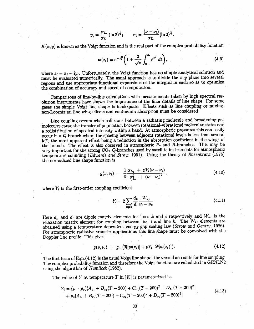
i = (ln2); i = ln2)aD, aDi

K(x, y) is known as the Voigt function and is the real part of the complex probability function

w(zi) = ez 1 + ; e' t dt) (4.9)

where zi = Xi + iyi. Unfortunately, the Voigt function has no simple analytical solution andmust be evaluated numerically. The usual approach is to divide the x, y plane into severalregions and use appropriate functional expansions of the integral in each so as to optimizethe combination of accuracy and speed of computation.

Comparisons of line-by-line calculations with measurements taken by high spectral res-olution instruments have shown the importance of the finer details of line shape. For somegases the simple Voigt line shape is inadequate. Effects such as line coupling or mixing,non-Lorentzian line wing effects and continuum absorption must be considered.

Line coupling occurs when collisions between a radiating molecule and broadening gasmolecules cause the transfer of population between rotational-vibrational molecular states anda redistribution of spectral intensity within a band. At atmospheric pressures this can easilyoccur in a Q-branch where the spacing between adjacent rotational levels is less than severalkT, the most apparent effect being a reduction in the absorption coefficient in the wings ofthe branch. The effect is also observed in atmospheric P- and R-branches. This may bevery important for the strong CO2 Q-branches used by satellite instruments for atmospherictemperature sounding (Edwards and Strow, 1991). Using the theory of Rosenkranz (1975)the normalized line shape function is

g(, i) = . l £ + p (4.10)ir a2 + (V -i)

where Yi is the first-order coupling coefficient

Y= 2E k Wki 2 (4.11)kTi d vi- vkkqi

Here dk and di are dipole matrix elements for lines k and i respectively and Wki is therelaxation matrix element for coupling between line i and line k. The Wki elements areobtained using a temperature dependent energy-gap scaling law (Strow and Gentry, 1986).For atmospheric radiative transfer applications this line shape must be convolved with theDoppler line profile. This gives

9(Y,Yi) = go,(Yt[w(zi)]+pYi 9[w1(Zi). (4.12)

The first term of Eqn.(4.12) is the usual Voigt line shape, the second accounts for line coupling.The complex probability function and therefore the Voigt function are calculated in GENLN2using the algorithm of Humlicek (1982).

The value of Y at temperature T in [K] is parameterized as

Yi = (p - p)[Aa, + Ba,(T - 200) + Ca,(T - 200)2 + Di(T - 200)]

+p,[A,, + B,, (T - 200) + C, (T - 200)2 + D, (T - 200) 3]

33

where the parameters with the subscript a account for air-broadening, those with subscript sfor self-broadening. This description of line coupling has been incorporated into the GENLN2model. The parameters A, B, C, and D are stored in block data subroutine LINMIX for theC02 Q-branches at 617, 667, 720, 740, and 791 cm-t. The Y coefficient is calculated at thesame time that line strength and half width are adjusted for the temperature and pressureof the atmospheric path under consideration. Y is then carried in the code as an extra lineparameter until the line profile is calculated according to Eqn.(4.12).

The sub-Lorentzian nature of the far wings of C02 lines is well known (Cousin et al.,1985, and references therein). Usually, the line shape function g(v, vi) based on the impacttheory is multiplied by a corrective factor X to give an empirical line shape

g(, asi)empir ic atl = g(c, i) x(t, vi). (4 .14)

The X-factor is a correction to account for the finite duration of collision between the broad-ening gas and the radiating molecule. This is assumed instantaneous in the impact approxi-mation which forms the basis of most collision broadened lined shape theories. It also includesthe effect of line coupling far from band center since the X-factor essentially represents thedifference between measurement and Lorentzian line wing theory. The factor usually takesthe form of an exponential with adjustable parameters and decays and from unity at line center.These parameters have traditionally been chosen by fitting the calculated absorption to themeasured absorption in the region above the C02 v3 band head at 4.3 pm. The X-factorscalculated in this region are often used in C02 line shapes at other vibrational bands. Theuser should be aware that the component of the factor due to line coupling will then be inerror as it is dependent on the symmetry of e the vibrational levels connected by the transitionthrough the number of available final rotational states. This is not usually a problem as theexponential part of the X-factor due to duration of collision effects quickly dominates thecontribution due to coupling. Birnbaum (1979) suggested a X-factor comprising the productof a decaying exponential to account for the finite duration of collisions alone and a constantterm for line coupling. The exponential term should be band independent while the constantcoupling term will not. This is discussed further in Edwards and Strow (1991).

GENLN2 includes a CO2 line shape option that includes the effect of line coupling andsub-Lorentzian line wings. If data is available, line coupling is included explicitly according toEqn.(4.12) out to an arbitrary 10 cmnl from line center. The line wings at greater distancesfrom line center are modified by the temperature dependent x-factor of Cousin et al. (1985).If line coupling data is not available then this sub-Lorentzian line shape is used everywhere.

4.4 Molecular Cross-Section Data

High resolution cross-section data are used to calculate absorption by molecules for whichline data is not available. These molecules and the molecular ID's assigned to them are listedin Table 2.1. The data sets currently used are temperature dependent cross-sections for theCFCs (McDaniel et al., 1991), N20 5 (Cantrell et al., 1988), CION0 2 (Ballard et al., 1988)and the room temperature sets acquired at the University of Denver (Massie et al., 1985).The temperature dependent data are a significant improvement over room temperature dataand allow greater confidence in the results. When only room temperature data are available,the cross-section is scaled by the ratio of the total internal partition function evaluated at296 K to that evaluated at the path temperature. Cross-sectional data is very importantfor modelling many of the heavy molecules of interest in atmospheric studies and althoughthe method is only approximate, the errors are considerably less than if the absorptioncontribution of these molecules is neglected.

34

4.5 The Line-By-Line Calculation

The line-by-line calculation involves calculating transmittances over the spectral range ofinterest in wavenumber space for each gas in several atmospheric layers. The simplest proce-dure is to choose a wavenumber grid fine enough that the narrowest line is adequately sampled,typically 0.0005 cm-1. Then for each line i of path gas j taken in turn the monochromaticabsorption is calculated at each grid point over the whole wavenumber range. The absorptioncoefficient at a wavenumber v can be written as the sum over the absorption contributionsfrom all lines i in the spectral range,

k(v)j= E Si g(v,vi)j. (4.15)all lines i

Here Sij is the strength of line i adjusted to the conditions of path j and g(v, vi)j is the lineshape function for line i. The total transmittance of a mixed path comprising J single gaspaths over several layers of the atmosphere is then

r(v)= exp(- k(v) u, (4.16)j=i

where the path gas amount uj per cross-sectional area in molecules.cm- 2 is defined inEqn.(3.2). Eqn.(4.16) is the approximation used to calculate the integral of Eqn.(1.3). InGENLN2 the line strength is scaled by the Avagadro number (6.022 x 1026) in programHITLIN to avoid underflow problems with very weak lines. To compensate for this, the unitactually used by the code for gas amount is kg.moles.cnm2 .

To calculate the absorption coefficient for every line at every wavenumber grid point isprohibitive for most applications and represents an excessive amount of computer time andstorage. Most algorithms that speed up the computation work on the basis that a widerwavenumber grid may reasonably be used in the wings of lines whilst a fine grid is requiredover the line center where the line profile is changing rapidly. The calculation also only needsto be performed for lines of significant strength.

In GENLN2 the spectral calculation is fully specified by the user input. The wavenum-ber range is first divided into a number of wide mesh intervals, Fig.4.1, which may be ofconstant or variable spacing. The line-by-line multi-path calculation proceeds in two stages.For each gas path a 'wide-pass' is first made over the total spectral range. For each widemesh in turn, the absorption due to the wings of lines whose centers fall into the range FEXC

to FwvND [cm - ' ] from the wide mesh boundaries are computed at the lower boundary, cen-ter, and upper boundary of the interval. The absorption contribution of the wings of lineswhose centers are further than FWIND [cm - 1 ] from the wide mesh boundary are included bymeans of a pre-computed temperature dependent continuum described in the next section.The contribution of far line wings and of lines lying outside of the wavenumber range ofinterest is importa t, especially near strong absorption bands (Fischer et al., 1988). Whenthe absorption contributions from all far-off line wings have been considered, a quadraticinterpolation between the three values at the wide mesh wavenumber points gives the totalline wing absorption at intermediate points.

A 'fine-pass' is then made over a fine wavenumber grid obtained by sub-dividing thewide mesh interval into many smaller intervals. This absorption calculation is performed forclose lines where the line shape may be changing very rapidly. All lines whose centers liewithin FEXC [cm Il of the wide mesh boundaries are included. The number of fine grid pointswithin each wide mesh interval defines the resolution of the calculation and is determined bythe width of the narrowest line encomuntered.

35

The interpolated wide-pass absorptions at the fine grid wavenumber points are thenadded to the fine-pass absorptions at these same points. This gives the line absorption totalswithin each wide mesh interval.

GENLN2 includes a line selection so that the line-by-line calculation is not performedfor extremely weak lines. The minimum line strength is determined as follows. An Elsasserdistribution of lines (Goody and Yung, 1989) of half width 0.1 cm - ', peak separation 0.01cm- ' and constant strength S, is assumed to represent the extreme case of a tight absorptionband of low optical depth. If for path j, the transmittance of such a line distribution is greaterthan 0.99999 then the lines are not considered significant. This condition implies a minimumvalue of SjUj for the line to be used. The wide-pass stage of the calculation rejects linesfor which SjUj < 10- 7 and the fine-pass stage rejects lines for which Sjuj < 10-8. Thesevalues are set in subroutines WIDEPS and FINEPS with the variable STMIN. To performthe calculation using all lines STMIN should be set to zero. The user should be aware thatthis condition for line rejection is only relevant for lower and middle terrestrial atmospherestudies and should be changed if GENLN2 is used for other applications.

Transmittances are required over the spectral range of interest for each single gas pathin the several tens of atmospheric layers. To store the absorption coefficients for the wholespectrum for all paths would result in prohibitively large array sizes. GENLN2 performsa 'vertical' calculation in that the absorption coefficients are calculated for all paths in alllayers but are only stored for each wide mesh interval before being written to output. Thusat any one time the monochromatic optical depths of all gas paths in all layers are known forone wide mesh interval.

4.6 Continuum Absorption

In addition to line-by-line absorption, the continuum absorption of certain molecules,in particular water vapor, must also be considered. This is especially important in remotesensing applications which utilize the infrared atmospheric windows around 4 pm and at 8-12/m. The H 2 0 continuum is responsible for most of the absorption in these regions and thelarge seasonal and zonal variations in the H2 0 mixing ratio in the troposphere can lead to awide range of calculated attenuations.

The continuum absorption has sometimes been called "anomalous" absorption becauseit is not accounted for by line shapes based on simple collision broadening theory and havingLorentzian wings. It may be considered as making up the difference between the observedabsorption and that resulting from a sum over all H 2 0 spectral lines in the atmosphericwindow regions that are located near to strong water bands. Thus its definition will dependon the reference line shape chosen, and this, along with the spectral region of interest, willdetermine if the continuum represents a "surplus" or "deficit" of absorption. The continuumformulation is therefore inextricably linked to the line shape description and the lack offormal agreement on definition has led to confusion and hindered comparison of differentmodels (Clough et al., 1989b).

Despite much effort, there is still no comprehensive theory to account for the contin-uum. It is essentially broadband, decreases rapidly with temperature and in the 8-12 p/mwindow, is much stronger for pure water vapor where self-broadening effects are importantthan for air-broadened lines. Fig. 4.2 shows the continuum contribution to the total radi-ance for a zenith view at sea level in a tropical atmosphere. There have been two generaltheories for explaining the continuum; the far spectral line wing absorption by water vapormonomers, and the absorption by water vapor dimers (Bignell, 1970; Gebbie, 1982). The neg-ative temperature dependence is suggested as possible evidence for the dimer theory (Suck,1982; Varanassi, 1988) since dimer populations would be expected to decrease rapidly with

36

increasing temperature. However, spectral features of the dimer are not observed in the wa-ter vapor continuum (Burch, 1982), and the theory would require a strong dimer absorptionband everywhere that the continuum is found. Measurements on saturated water vapor alsosuggest that dimer absorption is an of magnitude too small to account for the observations(Hinderling et al., 1987).

Recent studies have concentrated on explaining the far wing contributions to the watervapor absorption and to understanding the intermolecular potential and duration of collisionwhich determine absorption in this part of the line profile. Total line shapes that includeempirically fitted parameters have been developed by a number of authors (Clough et al.,1980; Thomas and Nordstrom, 1985; Rosenkranz, 1985, 1987; Ma and Tipping, 1990), andthese have met with some success in reproducing the continuum magnitude, frequency andquadratic pressure dependences, as well as the relative effectiveness of self-broadening com-pared to foreign-broadening. The strong negative temperature dependence remains a prob-lem, although advances have been made recently with the work of Rosenkranz, extended byMa and Tipping. This is able to produce a strong temperature dependence that is consistentwith observations in the far-wing.

Laboratory studies of water vapor continuum absorption using a spectrometer are madedifficult by the long paths required, and most (notably those of Burch) have been of necessityconducted at temperatures of 296 K or higher. Atmospheric temperatures are usually con-siderably lower, and due to the strong temperature dependence of continuum absorption alarge degree of uncertainty exists if, as is usual, an exponential relation is used to extrapolatemeasurements above 296 K to lower temperatures. Measurements in the atmosphere aretherefore very useful but few in number. A review of atmospheric and laboratory measure-ments is given by Grant (1990). For a more detailed discussion of continuum modelling seeKilsby et al. (1992).

The need for a continuum absorption parameterization that can be used in radiativetransfer models has led to the semi-empirical approach being adopted. The model of Cloughet al. (1980, 1989b) has been used in the Air Force Geophysics Laboratory codes FAS-CODE (Clough et al., 1989a), LOWTRAN (Kneizys et al., 1988), and is used in GENLN2.It describes the far line wings using the Van Vleck and Huber impact approximation lineshape modified by an empirically determined factor to fit the calculated absorption to theexperimental data of Burch and Alt (1984).

The continuum absorption coefficient kc(v) due to all lines i is defined by

k(v) =v tanh( 2 ) vi tanh(hcvi/2kT) (Yc( , vi) X(V, vi) + 9(-vi) X(-, 'i))

(4.17)where

gc( ±, i) = ( 2 for (v vi) > 25cm-, (4.18)ir a( + (V±Vi) 2

andgc(±VVi) = 1 aL for (v vi) I < 25cm-. (4.19)

ir a4 + 252

This description includes a constant continuum component over the line center region toavoid a discontinuity at 25 cm-' from line center. This component must be rememberedwhen performing the line-by-line calculation out to 25 cm - 1 from line center so that it is notcounted twice.

Eqn.(4.17) may be writtenkcc(=) =v tanh(hcv/2kT) C(v) (4.20)

37

where C(v) is the wavenumber dependent continuum parameter. For water vapor in theinfrared, X = 1 within about 5 cm- ' of the line center. At greater distances up to about500 cm - ' the line shape becomes super-Lorentzian. The X factor is dependent on (v - vi)and approaches values as high as 10 for the self-broadened case. At greater distances still theline becomes sub-Lorentzian. Similar behavior is found in the air-broadened case though toa lesser extent, with X > 1 up to about 100 cm - ' from line center.

Applying this definition of the continuum, the total continuum contribution to the ab-sorption coefficient kc(v) at some wavenumber v can be written

-r C, -kc() = tanh(hcv/2kT) ( C T)+ (P -) Cf(vT) (4.21)

T 1 / Pre! Pref

C ° is the continuum absorption parameter for the self component and Cf is the parameter forthe foreign component, both have units of 1/(cm- .molecules.cm- 2). C O and Cf are definedat a reference pressure, and the temperature and pressure factors in Eqn.(4.21) take intoaccount the density dependence of the self and foreign broadened line half widths. Valuesof C O are stored in the code at temperatures of 260 K and 296 K. The strong negativetemperature dependence is obtained by exponentially extrapolating between these values atthe required wavenumber. Due to a lack of measurements at lower temperatures, the 260K data is an extrapolation of Burch's measurements at 296 K and 338 K and as such is apotential source of error. The temperature dependence of Cf has not been determined androom temperature values are used.

The line-by-line part of the GENLN2 calculation takes into account line wings up to25 cm-' from the line center. The pre-computed continua described here account for theabsorption contribution of the line wings at greater separations.

In addition to H 20, a C02 continuum is also included. This has been calculated usingthe GENLN2 CO 2 line shape. The continuum is stored in the code at temperatures of 230K, 250 K and 296 K and the absorption at a particular path temperature is obtained byinterpolation between these values at the required wavenumber.

The pressure broadened band of N2 at 2350 cm-' (Clough et al., 1981) and that of02 at 1550 cm-' (Titnofeyev and Tonkov, 1978; Rinsland et al., 1989) are also included asbroad-band continuum contributions to the absorption. The same facility may be used toinclude other grey absorptions such as aerosols.

4.7 Transmittance Calculations

Having calculated the various components contributing to absorption at the fine gridwavenumber points for some path j, the total monochromatic absorption coefficient may beformed,

k(v)j = k(v)"l e- n + k(v)?e ines + k(v)o . (4.22)

The broadband absorption includes the continuum and molecular cross-section contributions.The monochromatic optical depth of the path is given by the product of the absorptioncoefficient and the total path absorber amount, k(v)juj. At this stage the optical depthsof the various single gas paths may be combined to obtain multi-gas optical depths andoptical depths over several layers according to the problem being addressed. This operationis performed in GENLN2 by a device called a mixing table, here represented by the matrixM. The elements Mm,j specify the contribution that each path optical depth k(v)juj is tomake in forming the mixed path optical depth K(v)m for some mixed path m. If there

38

are Nm mixed path absorptions to be formed from the Np computed path absorptions thecalculation takes the form,

K(I v) Ml,1 Ml,2 ... M1,N \ k(v)1iUK(v)2 2,1 M2,2 ... M2,Np k k(v)22

(4.23): - : ; -. : e e e

K(V)N \MN,,I MN.,2 .. MN,,NpJ k(v)N

This calculation is performed over each point of the fine wavenumber grid. The transmittanceof each mixed path is then calculated according to

T(V)m = exp(-K(v)m). (4.24)

The mixing table is a versatile device which allows for economy of calculation of many at-mospheric mixed paths. For example, slant path calculations through the atmosphere for aseries of small angles may be simply performed by multiplying the vertical path absorptionsby secO, where 0 is the local zenith angle. Such a calculation does not take into accountrefraction effects but this is not found to be a serious source of error for values of 0 less thanabout 60°. It represents a considerable economy of calculation when several slant path viewsfor the same atmospheric profile are to be computed. The mixing table is also very usefulfor performing several transmittance calculations in parallel for slightly different atmosphericprofiles. If the profiles have paths in common then the optical depths of these need only becomputed once and combined with the path absorptions of other gases in the mixed paths asrequired. An application of this might be in determining the sensitivity of the atmosphericabsorption to differing amounts of one particular gas, the mixing ratio profiles of the othergases remaining constant.

An example mixing table is shown in Fig.4.3 along with an illustration of the mixedpaths it calculates. The table uses the set of 15 paths shown in the example of Fig.3.1.Mixed path 1 shows how the optical depths of several layers may be combined for a singlegas. This mixed path may be used to find the transmittance of the atmosphere due to watervapor alone. Mixed paths 2-4 are for a calculation to investigate the attenuating effect ofmixed gas absorption from different levels in the atmosphere. Mixed paths 5 and 6 representa slant path calculation for a zenith angle of 0 = 45°. Mixed paths 7-11 calculate the totaloptical depth for each layer of the atmosphere. These mixed paths could be used to representthe layer in a GENLN2 radiance calculation in the way described in the next section. Theexample shown here is for a nadir viewing geometry. For a limb-viewing geometry the mixingtable is used to combine path optical depths for different gases within a layer and betweenlayers in the same manner.

4.8 Radiance Calculations

GENLN2 may be run in one of two modes, for transmittance calculations only or fortransmittance and radiance. A typical nadir viewing problem in satellite remote sensing mightbe the calculation of radiance at some altitude Zobs above the Earth due to the coi lbinedeffect of a radiating surface at z, such as the land, sea or cloud top and the thermal emissionof the atmosphere. In this case the radiative transfer equation from Eqn.(1.6) is

zobs

I(V, Zobs) = I(v, zs) T(Y, ZS Zobs) + [B( T(z)) k(, z)p(z) dz] Tr(V, Z, Zobs) (4.25)

Z's

where I(v, zs) is the intensity of radiation leaving the surface, p, is the density of the absorbinggas and B(v, T) is the Planck emission function at temperature T. In general I(v, z,) is given

39

by

I(v, z8) = E B(v, T) + (1 - E) (B(v, Tb) (,Zb, )

Z. (4.26)

+ i[B(, T(z)) k(v )(z) d] T(v, Z z))Zb

where E is the emittance and T, the temperature of the surface. The effective edge ofthe Earth's atmosphere is Zb, and Tb the temperature at this boundary. The first termof Eqn.(4.26) is the thermal emission of the surface. Assuming specular reflection, the secondterm represents the reflectance multiplied by the total radiation reaching the surface fromthe atmosphere. The latter is zero if the surface is a blackbody with e = 1. For a limb view-ing case looking into deep space, the observed radiance will be due to atmospheric thermalemission alone and will be given by a term similar to Eqn.(4.25) with the first term set tozero and Zb substituted for z 8.

In the GENLN2 radiance calculation the atmosphere is considered sub-divided into anumber of homogeneous layers. The total optical depth of each layer I is defined in theGENLN2 input from among the computed path optical depths, k(v)juj, or mixed pathoptical depths, K(v)m. Assuming that the layer is made up of J single gas paths, the totallayer optical depth b(v)l will be given by a mixed path m for which

J

0(v), K(v)m == k(v)juj, (4.27)j=1

and the layer transmittance isT(V)I= exp(-((v)l). (4.28)

Each layer also has an associated temperature T1 which is an absorption weighted mean of thepath temperatures that constitute the layer. For a layer in local thermodynamic equilibriumthis allows the layer thermal emission E(v)I to be defined from the integral in Eqn.(4.25) andEqn.(3.2) as

J fz1+E(v) = B(v,Ti) Zk(v)j pa, r(v (yz, Z+) dz

-j=i J zl (4.29)

= B(,T) () [1 - '(v)],

where J

f = Z k(v)juj. (4.30)j=l

The optical depth ratio (q(v)l//(v)L) is unity as it stands, but has been retained here todemonstrate how GENLN2 performs an emission calculation. It is often useful to know whatcomponent of the total radiance at some point in the atmosphere is due to the emission fromone particular gas species. For example, it is necessary to know how much of the measuredinstrument signal in a CO2 sounding channel is due to a contaminating 03 signal. Considera calculation to find the radiance due only to gas C when the atmosphere is composed ofgases A, B, C, and D. Whatever the emission source, it will be attenuated according to thelayer transmittance r(v)l which is defined by the layer optical depth Il of all the gases A,B, C and D. The optical depth of gas C alone is then used to define the layer emission, i.e.

40

0(v)l = k(v)cuc only. For such a GENLN2 calculation, the user must define in each layer,a total optical depth '(v)l and the emission source optical depth 0(v)l, by choosing fromamong the previously calculated path and mixed path optical depths.

The radiance calculation then proceeds in two stages. First Eqn.(4.26) for the radiationleaving the surface is evaluated if it is defined by the problem. The radiance at the point ofobservation is then calculated using Eqn.(4.25). In both cases the same step-wise algorithmis used to calculate the radiance at the furthest boundary of the Ith layer as

I(v), = I(v)i-I r(v)1 + E(v),. (4.31)

GENLN2 allows several radiance calculations to be performed at once. Each calculation isspecified by the layer optical depths which define the radiating atmosphere and the boundarytemperatures and emittances where appropriate.

4.9 Description of GENLN2 Subroutines

The GENLN2 program structure is shown in Fig.4.4.

GENLN2 - Main program. Management program for the calculation.

GENDAT - Block data subroutine. Initializes data for GENLN2 common blocks.

OUTDT1 - Subroutine. Initializes the formatted summary output data file and writes aheader. The output file will be used for any error messages written during theinput processing.

TIMER - SYSTEM SPECIFIC: Subroutine. This routine returns the system date and thecru run time at call. It relies on system specific function calls. It is suppliedin skeletal form and will require editing before it will perform its function.

INPUT - Subroutine. Main input routine to read the user's input data file which definesthe GENLN2 task. The routine searches the input for the *KEYWORD entriesand calls the relevant input subroutine to read the section.

TITLES - Subroutine. Reads the *TITLES title and output specification section of themain input file.

GASFIL - Subroutine. Reads the *GASFIL line data file information section of the maininput file.

XSCFIL - Subroutine. Reads the *XSCFIL molecular cross-section information section ofthe main input file.

USEGRD -

DEFGRD -

RADIOM -

Subroutine. Reads the *USEGRD and *GRDFIL sections of the main input file.Opens and reads the user's data file defining the wavenumber boundaries ofthe wide mesh intervals.

Subroutine. Reads the *DEFGRD section of the main input file and calculatesthe wavenumber boundaries of the wide mesh intervals.

Subroutine. Reads the *RADIOM section of the main input file. Opens andreads the user's data file containing wavenumber boundaries of the wide meshintervals and the values of the radiometer filter response mask.

SPECTM - Subroutine. Reads the *SPECTM spectral calculation definition section of themain input file.

41

PTHFIL - Subroutine. Reads the *PTHFIL section of the main input file. Opens andreads the user's path data file from the output of program LAYERS.

PTHPAR - Subroutine. Reads the *PTHPAR path data section of the main input file.

MIXING -

RADNCE -

OUTPUT -

OUTDT2 -

WIDEPS -

Subroutine. Reads the *MIXING and *MIXFIL sections of the main input file.Opens and reads the user's mixing table data file.

Subroutine. Reads the *RADNCE and *RADFIL section of the main input file.Opens and reads the user's radiance input data file.

Subroutine. Reads the *OUTPUT output data specification section of the inputfile.

Subroutine. Writes a summary of the input file data just read to the formattedsummary output data file.

Subroutine. Performs the line-by-line wide-pass absorption calculation forabsorption due to the line wings over all the wide mesh wavenumber intervalsand for all paths. If the fine grid wavenumber interval is being chosen accordingto the minimum line width encountered, i.e. NDIV< 0 in the *SPECTM sectionof the input file, then this minimum line width adjusted for path conditionsis found and used to calculate the fine grid spacing in each wide mesh.

HITINI - Subroutine. Initializes the reading of the line data file(s) containing the lineparameters (output of the HITLIN program).

HITRD - Subroutine. Reads the line data file and returns the line parameters of awanted gas.

LINMIX - Block data. Contains the parameters for the line coupling calculation.

PTHADJ - Subroutine. According to the gas path conditions, this routine calculates thepressure and Doppler broadened widths, strength and line coupling coefficientfrom the parameters of the last line read from the line data file. If isotopeabundances other than those of the terrestrial atmosphere are to be used, theyshould be set in this subroutine.

ISOTPE - Block data. Contains the HITRAN isotope masses and abundances.

QTFCT - Subroutine. Calculates the total internal partition function for the moleculesincluded on the HITRAN data base given the given molecular species and thetemperature.

QTIPS - Block data. Data for the calculation of total partition function. This is essen-tially the TIPS program of Gamache et al. (1990).

QTIN T- Subroutine. Calculates the total internal partition function for gases otherthan the 32 included on the HITRAN data base, i.e. the heavy molecules forwhich only cross-section data are available.

QSHEV - Block data. Data for the calculation of the total internal partition function ofthe heavy molecules.

CONSUB- Subroutine. This routine calculates the absorption component over the linecenter that is included in the Clough et al. (1980, 1989) definition of the H 20

42

continuum. This component is not then included in the GENLN2 line-by-linecalculation when a continuum calculation is involved.

LORNTZ - Subroutine. Calculates the absorption assuming a Lorentz line profile over thewide mesh interval.

VOIGT - Subroutine. Calculates the absorption assuming a Voigt line profile over thewide mesh interval.

VOIVEC - Subroutine. Calculates the complex probability function using a vectorizedversion of the Humlicek (1982) routine.

NEWSHP - Subroutine. This is a skeleton routine which the user can modify for their ownline shape function which is than calculated over the wide mesh interval.

VOIC02- Subroutine. Calculates the absorption assuming a Voigt line profile modi-fied for CO2 sub-Lorentzian line wings and line coupling over the wide meshinterval.

VANHUB - Subroutine. Calculates the absorption assuming the modified Van Vleck andHuber line profile over the wide mesh interval.

DOPLER- Subroutine. Calculates the absorption assuming a Doppler line profile overthe wide mesh interval.

CONTUM- Subroutine. Calculates the continuum absorption over all the wide meshwavenumber intervals for specified paths.

CO2FTO - Block data. C02 continuum coefficients at 296 K.

CO2FT1 - Block data. C02 continuum coefficients at 260 K.

C02FT2 - Block data. CO2 continuum coefficients at 230 K.

H20STO - Block data. H20 self-density dependent continuum coefficients at 296 K.

H20ST1 - Block data. H20 self-density dependent continuum coefficients at 260 K.

H2OFTO - Block data. H20 foreign-density dependent continuum coefficients at 296 K.

N2CTO - Block data. N2 collision induced continuum coefficients at 296 K.

02CTT - Block data. 02 collision induced continuum coefficients at 293 K, 253 K and213 K.

OUTGR1- Subroutine. Opens the unformatted output data file specified in the*OUTPUT section of the input file and writes a summary of the input filedata.

WINGCO - Subroutine. Interpolates the wide-pass and continuum absorptions calculatedat the three wavenumber points of the current wide mesh interval onto thefine grid of the interval for all paths.

XSECAB- Subroutine. Calculates the absorption by path and wide mesh interval forthose heavy molecules whose absorption is represented by molecular cross-sections. This routine uses the cross-section absorption data file xsec.dat.

43

FINEPS- Subroutine. Performs the line-by-line fine-pass calculation of the absorptiondue to near lines at the fine grid wavenumber points of the current wide meshinterval and for all paths.

CYCRD - Subroutine. Manages the cyclic buffers of line parameters for lines that con-tribute to the fine-pass line-by-line absorption calculation over the fine gridwavenumber points in the current wide mesh interval.

BUFSWP -

TRINTG -

MIXPTH -

OUTGR2 -

Subroutine. Stores the line parameters for the last line read in the currentcyclic buffer range for a particular line data file before bringing into play theline parameters of the first useful line of the next line data file being used.

Subroutine. General purpose integration routine using the trapezium rule.Used to integrate the radiometer response function, path, mixed path, andlayer transmittances and radiances over each wide mesh interval.

Subroutine. Performs the mixed path absorption calculation for all mixedpaths over the fine grid of the current wide mesh interval. Uses the mixingtable and path absorptions already calculated. A path absorption weightedmean temperature is also calculated to represent the temperature of eachmixed path.

Subroutine. Writes to the unformatted output data file the specified path andmixed path transmittances at the fine grid wavenumber points of the currentwide mesh interval.

EMISSN- Subroutine. Performs the transmittance, emission and radiance calculationon the fine wavenumber grid for all layers of the current radiating atmosphereand wide mesh interval.

PLANCK -

OUTGR3 -

OUTDT3 -

OUTGR4 -

Subroutine. Calculates the Planck function at given temperature over the finewavenumber grid for the current wide mesh interval.

Subroutine. Writes to the unformatted output data file the specified atmo-sphere and layer transmittances and radiances over the fine wavenumber gridfor the current wide mesh interval.

Subroutine. Writes to the formatted output file the specified spectra binnedand integrated over the current wide mesh interval.

Subroutine. Writes to the unformatted output file the specified spectra binnedand integrated over the current wide mesh interval.

4.10 Description of the GENLN2 Input File

Input to GENLN2 is by means of a user supplied input file in the standard formatdescribed in Section 1.3. This is assigned to FORTRAN unit number 4 before execution com-mences. Table 4.1 gives details of the input file. The different *KEYWORD sections aredescribed below.

*TITLESThis section is mandatory.(1A) TITLE (40 character string) is the title of the GENLN2 run. This is used as a headerfor the output files and should be descriptive.(2A) AVER (logical) is a print switch to reduce the amount of output in the formatted

44

summary output file. If AVER is set to .TRUE. then the printing of the average spectral valuesbinned over each wide mesh is suppressed and only the average value over the full passbandrange is printed. If AVER is set to .FALSE. then the full data is output.(2B) MXER (logical) is also a print switch. If it is set to .TRUE. then the mixing table is notreproduced in the summary output file. Remember that mixing tables can get very large!

Next comes the input that will specify which transmittances and radiances are writtento the formatted summary output data file as it is unlikely that all the possible GENLN2output will be needed.(3A) IDAT (integer) allows the path, mixed path or layer transmittance and radiance in-tegrated spectra to be chosen. These three categories take the values IDAT= 1, 2, and 3respectively.(4A) IATM (integer) specifies the relevant atmosphere number (radiance calculation number)when IDAT= 3. For IDAT= 1 or 2 this is absent. Setting IATM< 0 results in spectra for allatmospheres being printed.(4B) NP (integer) specifies the number of paths, mixed paths or layers to be printed. If NP< 0then all are printed.(5A) IOPDT (integer) gives the list of NP (if NP> 0) path, mixed path, or layer numbers to beprinted. 5A is absent if NP< 0. The above input parameters are repeated as required, eachtime beginning at the value of IDAT.

In the output section here and in *OUTPUT which specifies the spectral output that willbe written to the GENLN2 unformatted output file, a path or mixed path transmittance isthe transmittance calculated over the specified path or mixed path. The layer transmittancecalculated during the the radiating atmosphere calculation refers to the total transmittancefrom the initiating boundary of the atmosphere to the furthest boundary of the specified layerin the direction of radiation travel along the ray path. The radiance is also reported at thissame layer boundary. Note that layers for a radiance calculation are numbered sequentiallyin the direction of radiation travel with the initiating surface of the radiating atmosphereforming the lower boundary of layer 1.

*GASFILThis input section is mandatory and specifies where the line data files are to be found andwhich gas lines are to be read from which file. These line data files are the unformatted directaccess files produced as the output of the program HITLIN.(1A) NFILE (integer) specifies the number. of line data files to be used. NFILE must be lessthan or equal to MXFIL in the PARRAY statement.(1B) MACH (integer) is a machine specifier that determines the record length of the linefile. For a machine that has a 4 byte per word representation and defines the FORTRAN OPEN

statement RECL in words, MACH= 1. This is the ANSII standard and is used under VAX/VMS.

Other 4 byte per word machines specify the RECL in bytes, eg. IBM/RISC and MACH= 2. Forthe CRAY which has an 8 byte per word representation and defines RECL in bytes, MACH= 3.The same MACH value should be used here as was used by program HITLIN when the linefile was written.

The following section is then repeated NFILE times.(2A) FNAM (80 character string) is the file name of the line data file.(3A) NGAS (integer) specifies the number of gases to be read from the data file. NGAS mustbe less than or equal to MXGAS in the PARRAY statement.(4A) LGASES (integer) lists the NGAS molecular ID's of the gases to be read. These are theHITRAN molecular ID's given in Table 2.1.(5A) LCHOSE (integer) lists the line version parameters to distinguish between the versionsof duplicate lines on the data file. If LCHOSE= m then the most recent line versions up toand including the lines with status m are used. Only one version of any particular line will

45

be used in the line-by-line calculation. For example, program HITLIN may be used to mergethe HITRAN data base (identified as having status 10) with line updates of a particular gas(identified as having status 11 say). Where HITLIN encounters a duplicate line, the linewith the lower status number will have its status number set equal to the negative of itself.Thus the status number of a line on the HITRAN data base that has been updated will beset to -10. If the LCHOSE parameter for this gas is set equal to 11 then GENLN2 will uselines that have a status number greater than or equal to 10 and less than or equal to 11 orequal to -11, i.e. the lines used have a status number between 10 and LCHOSE inclusive orstatus equal to -LCHOSE. This will not include the HITRAN lines with status -10 that havebeen updated. However, if only HITRAN lines are required for the calculation the LCHOSEparameter can be set to 10 and only lines with status numbers of ±10 will be used.

*XSCFILThis section it not mandatory. It includes the input necessary to define an absorption calcu-lation for those molecules for which cross-section data files are used.(1A) NXSFIL (integer) is the number of cross-section data files to be used. NXSFIL must beless than or equal to MXFIL in the PARRAY statement. The following section is then repeatedNXSFIL times.(2A) FXSNAM (80 character string) is the cross-section data file name. The file xsec.dat isprovide.(3A) NXSEC (integer) is the number of gases for which cross-sections should be read from thecross-section file. NXSEC must be less than or equal to MXGAS in the PARRAY statement.(4A) LXSEC (integer) is a list of molecular ID's of the gases for which cross-sections are to beread from the file. Table 2.1 shows the molecular ID-gas pairings being used. For paths thatuse cross-section data, the (3A) LINSHP parameter in *PTHPAR or *PTHFIL takes the value'XSECTION'.

The cross-section data set is written in the NCAR format which will likely be adoptedfor the next edition of HITRAN on which these same cross-sections will be included. The filexsec.dat contains cross-sections for the molecules important for middle atmosphere studies.The header record and first line of the data are shown for the first few cross-section sets inTable 4.2.

*LINMIXLogical switch. This section is not mandatory and indicates that line coupling should beincluded where appropriate. Data is currently available for the CO2 Q-branches at 617, 667,720, 740, and 791 cm- 1, and is based on the CO2 line parameters in file CO2MIX. In creatingthe line data file for use with a GENLN2 run with line coupling, the lines on CO2MIX shouldform the line input to HITLIN with the highest status number. The CO2 LCHOSE value in*GASFIL should then be equal to this status number so that the required lines are selected.The 'VOIGTCO2' line shape should be used for the (3A) LINSHP parameter in *PTHPAR or*PTHFIL. In any computation with line coupling it is ESSENTIAL that the spectral rangeof the line-by-line calculation include all lines of the band for which coupling parameters havebeen calculated. This is to satisfy the line strength and coupling parameter sum rules (Strowand Reuter, 1988).

One and only one of the input sections *USEGRD, *GRDFIL, *DEFGRD or *RADIOM mustbe supplied. These sections perform the same task in setting up the spectral range to beinvestigated. The input wavenumber parameters are illustrated in Fig.4.1.

*USEGRDWith *USEGRD the user supplies the wide mesh interval boundary wavenumber grid to coverthe total spectral range of interest. Besides the passband wavenumber range, an adequatemargin on either side should be included if a line-wing absorption calculation is to be per-

46

formed.(1A) MINT (integer) is the number of wide mesh wavenumber intervals. MINT+1 must beless than or equal to MXINT in the PARRAY statement.(2A) FBDY (real) is the array of MINT+I wavenumber boundaries in cm- 1. The intervalboundaries do not have to be of equal spacing, but the spacing should not be greater than afew wavenumbers.(3A) NPL (integer) is index of the FBDY element corresponding to the wavenumber of thelower passband boundary.(3B) NPU (integer) is index of the FBDY element corresponding to the wavenumber of theupper passband boundary.

*GRDFILThis section allows the same input as the *USECRD section to be read from an external file.(1A) GRDFIL (80 character string) is the file name of the user's wide mesh interval boundarywavenumber file. The data on GRDFI should appear in exactly the same form as specifiedabove for *USEGRD beginning at input record 1.

*DEFGRDA default array of wide mesh interval boundary wavenumbers is calculated in this section.The intervals are calculated with constant spacing.(1A) FMIN (real) is the minimum wavenumber cmn1 of any line to be considered in theGENLN2 calculation.(1B) FPSL (real) is the lower passband wavenumber cm -1 .(1C) FPSU (real) is the upper passband wavenumber cm 1.(1D) FMAX (real) is the maximum wavenumber cmn- of any line to be considered in theGENLN2 calculation.(1E) DELTA (real) is the constant wide mesh interval spacing in cm - '. This should have avalue of about 1 cm-' for accurate interpolation of the wing absorption during the fine-passstage.

*RADIOMThis section is used to input a radiometer spectral filter for the GENLN2 calculation. Theoption is primarily of use in performing radiative transfer studies using gas correlation in-struments. The use of this option in Pressure Modulator Radiometer (PMR) calculations isdescribed in Appendix 3.

*SPECTMThis section is mandatory if *USEGRD, *GRDFIL or *DEFGRD are used but must not be usedwith *RADIOM. It supplies the spectral calculation parameters illustrated in Fig.4.1.(1A) FEXC (real) is the wavenumber range in cm-' either side of a wide mesh intervalfor which the fine-pass calculation is performed. For wide mesh interval IPW a line-by-lineabsorption calculation is performed over the fine wavenumber grid FF(IPT,IPW) for line centerwavenumbers WNUM cr- 1 falling in the rangeFBDY(IPW+NPL-1) - FEXC < WNUM < FBDY(IPW+NPL) + FEXC(1B) FWIND (real) is the wavenumber range cm - ' either side of a wide mesh interval outsideof which lines are not considered. The line wing absorption calculation is performed over thethree wavenumber points FW(IP,IPW) of the wide mesh for line center wavenumbers WNUMcm -r falling in the rangesFW(IP,IPW) - FWIND < WNUM < FBDY(IPW+NPL-1) - FEXC andFW(IP,IPW) +FWIND > WNUM > FBDY(IPW+NPL) + FEXC.FWIND should be set equal to 25 cm- 1 if a continuum absorption calculation is to be performedas discussed in Section 4.6.(1C) NDIV (integer) determines the spectral resolution of the calculation. If NDIV> 0 thenthe wide mesh interval is divided into NDIV fine mesh intervals over which the spectrum

47

is calculated. In this case NDIV+I must be less than or equal to MXDIV in the PARRAYstatement. The line-by-line calculation is then performed on a grid with spacing DELTA/NDIVcm-l. If NDIV< 0 then the wide mesh interval IPW is divided such that the fine mesh gridspacing is set equal to the minimum path adjusted line width encountered in the wavenumberrangeFBDY(IPW+NPL-1) - FEXC < WNUM < FBDY(IPW+NPL) + FEXCdivided by the absolute value of NDIV. This can lead to different fine grid spacing in differentwide mesh intervals. If the calculated spectra are to be convolved with an instrument functionin the GENGRP program, this option is not recommended (see the discussion of Section 5.3).

One at least of the input sections *PTHPAR or *PTHFIL must be supplied. The totalnumber of paths from all sources must be less than or equal to MXPTH in the PARRAYstatement.

*PTHPARThis section includes the information required to define the path conditions.(1A) NPATH (integer) specifies the number of paths to be read from this section. Thefollowing section is then repeated NPATH times.(2A) IDFIL (integer) indicates from which line data file or cross-section data file (IFILE value)the data for the path gas should be read.(2B) IDGAS (integer) is the molecular ID of the path gas. This should be the same as oneof the LGASES gases specified in section *GASFIL or one of the LXSEC gases in section *XSCFILfor file IDFIL.(2C) IDISO (Integer) is the HITRAN isotope abundance ID. This is defined as follows; forIDISO= 0 lines of all isotopes of the gas are considered, for IDISO= 1 lines of the 1st mostabundant isotope are taken, and so on. It should be remembered when specifying IDISO asanything other than 0 that the line strengths for a particular gas in the HITRAN data baseare weighted according to the terrestrial atmospheric isotope abundance.(2D) AMT (real) is the path integrated gas amount in units of kg.moles.cm 2.(2E) T (real) is the average path temperature in K.(2F) P (real) is the average path pressure in atm.(2G) PARTP (real) is the average partial pressure of the path gas in atm.(2H) VEL (real) is the path velocity relative to the line of sight in m.s-1 but is not yetimplemented and should be set to zero.3(A) LINSHP (8 character string) describes which line shape should be used for the path gas.At present the options are:

'LORENTZ' The Lorentz line shape;'DOPPLER' The Doppler line shape;

'VOIGT' The Voigt line shape using the Humlicek (1982) routine;'VANVHUB' The modified Van-Vleck Huber line shape (Clough et al., 1980);'VOIGTCO2' The Voigt line shape modified for sub-Lorentzian CO 2 line wing behavior

(Cousin et al., 1985) and line coupling (Edwards and Strow, 1991);'NEWSHAPE' For the user to supply their own line shape routine NEWSHP;

'XSECTION' If the calculation is to use cross-section data.(3B) CONT (8 character string) determines if a continuum calculation is to be performedfor this path and takes the value 'CON' or 'NOCON' appropriately. Continuum data areavailable for H20, CO2, and the N2 and 02 pressure broadened bands.

*PTHFILThis section allows the same input as the *PTHPAR section to be read from an external file.(1A) PFNAM (80 character string) is the file name of the user's path data file. The data onPFNAM should appear in exactly the same form as specified above for *PTHPAR beginning atinput record I. This section is used to input the path data calculated by program LAYERSwhich is already in the required format and can be used directly. The *PTHFIL section can

48

be included several times to allow for more than one LAYERS output path file to be used.The paths are then numbered sequentially in the order that they are read.

*MIXINGThis section defines the mixed path calculation. It is not mandatory and must not be suppliedwith *MIXFIL.(1A) NPMIX (integer) specifies the number of mixed paths to be calculated. NPMIX must beless than or equal to MXPMX in the PARRAY statement. This is followed by the mixing tableitself.(2A) IPMIX (integer) is the mixed path number.(2B) TABMIX (real) is the mixing table. The table has NPMIX rows and NPATH columns. Theinput fields can be up to 130 characters wide. Remember that NPATH here is the sum of allthe paths read in the *PTHPAR and *PTHFIL sections. The entries for a particular mixed pathmay run over several lines of the input file, and input for a new mixed path must begin anew line.

It is often the case when mixing many paths together that a whole string of zeros or someother number must be entered in the table. In this case, an alternative to typing a numberx n times is to type RxTn. So for example a line of input 0, 0, 0, 0, , could be writtenROT5. This reduces the physical size of the mixing table and helps prevent input errors. Themixing table entries should be written either as integers or F format real numbers.

*MIXFILThis section allows the same input as the *MIXING section to be read from an external file.It is not mandatory and must not be specified with *MIXING.(1A) MIXFI (80 character string) is the file name of the user's mixing table file. The data onMIXFI should appear in exactly the same form as specified above for *MIXING beginning atinput record 1.

*RADNCEThis section is included if a radiance calculation is required. It is not mandatory and mustnot be specified with *RADFIL.(1A) NATM (integer) specifies the number of different radiance ('radiating atmosphere') cal-culations that are to be performed. NATM must be less than or equal to MXATM in thePARRAY statement. The following section is then repeated NATM times.(2A) IATM (integer) is the atmosphere index.(2B) IVIEW (integer) is the viewing parameter. This can take two values which determinethe boundary condition to be used in the radiation transfer equation as discussed in Section4.8. If IVIEW= 1 then the radiance at the inward boundary to the first layer is set equal tozero. This would be appropriate to a limb emission calculation. If IVIEW= 2 a radiating sur-face boundary condition is applied. This would be appropriate for a nadir sounding problemwhere the surface emission term is non-negligible.(2C) IEMS (integer) is the layer emission parameter. If IEMS= 1 then a single optical depthis later specified for each layer and this is used to determine both the layer transmittanceand emission, i.e. )(v)l and k(v)l in Eqn.(4.29) are identical. Setting IEMS= 2 specifies anemission calculation and two optical depths are required for each layer, one to determine thelayer transmittance ?(v)l, and the other to determine the layer emission O(v)l.(2D) NLAY (integer) specifies the number of layers for the atmosphere. NLAY must be lessthan or equal to MXLAY in the PARRAY statement.(2E) LAYSP (integer) indicates if the set of indices that follow (LAYER) for specifying the layeroptical depth for the transmittance calculation b(v)lj (and emission calculation if IEMS= 1)refer to path numbers, LAYSP= 1, or mixed path numbers, LAYSP= 2.(2F) LAYER (integer) are a list of NLAY indices referring to the path numbers (LAYSP= 1)or mixed path numbers (LAYSP= 2) whose optical depth are to be used to define the optical

49

depths I(v)i of the layers for the layer transmittance calculation. The indices defining eachlayer should be listed in the direction of radiation travel through the atmosphere.

If IVIEW= 2 then the parameters defining the radiating boundary surface come next. IfrvIEW= 1 this section is absent.(3A) TBDY (real) is the temperature of the atmospheric boundary furthest away from thereflecting surface. For example in the case of a nadir viewing satellite, TBDY= 2.96 K thetemperature of cold space and the effective top of the atmosphere. This corresponds to thequantity Tb in Eqn.(4.26).(3B) TINIT (real) is the boundary surface temperature corresponding to T8 in Eqn.(4.26).(3C) EMSTY (real) is the surface emittance corresponding to e in Eqn.(4.26).

If IEMS= 2 then a different set of optical depths, q(v)i in Eqn.(4.29), are required todefine the layer emission. If IEMS= 1 then this section is absent.(4A) LEMSP (integer) indicates if the set of indices that follow (LAYEMS) for specifying thelayer optical depth 0(v)l for the emission calculation refer to path numbers, LEMSP= 1, ormixed path numbers, LEMSP= 2.(4B) LAYEMS (integer) are a list of NLAY indices referring to the path numbers (LEMSP= 1)

or mixed path numbers (LEMSP= 2) whose optical depths are to be used to define the opticaldepths b(v)l of the layers for the layer emission calculation. The indices defining each layershould be listed in the direction of radiation travel through the atmosphere.

*RADFILThis section allows the same input as the *RADNCE section to be read from an external file.It is not mandatory and must not be specified with *RADNCE.

(1A) RADFI (80 character string) is the file name of the user's radiance input data file.The data on RADFI should appear in exactly the same form as specified above for *RADNCE

beginning at input record 1.

*OUTPUTIf *OUTPUT is specified then an unformatted output file will be written. It is not mandatory.This file is in addition to the formatted summary output data file that is assigned prior toexecution and for which output data selection is made in *TITLES. As this file is for graphicsuse, there is provision for output of the point spectra calculated on the fine wavenumber gridas well as the binned spectra integrated over the wide mesh intervals.(1A) OPFNAM (80 character string) is the file name of the output file.(2A) IDAT (integer) is an output selection parameter similar to that used in the *TITLES

section. For the different output categories this now takes the values:1. for the path point transmittance spectra;2. for the path integrated transmittance spectra;3. for the mixed path point transmittance spectra;4. for the mixed path integrated transmittance spectra;5. for the radiating atmosphere layer point transmittance spectra;6. for the radiating atmosphere layer integrated transmittance spectra;7. for the radiating atmosphere layer point radiance spectra;8. for the radiating atmosphere layer integrated radiance spectrum.

(3A) IATM (integer) specifies the relevant atmosphere number (radiance calculation number)when IDAT> 4. For IDAT< 4 it is absent. Setting IATM< 0 results in spectra for all atmospheresbeing written.(3B) NP (integer) specifies the number of paths, mixed paths or layers to be written. If NP< 0then all are written.(4A) IOPGR (integer) gives the list of NP (if NP> 0) path, mixed path, or layer numbers tobe written. 4A is absent if NP< 0. The above input parameters are repeated as required eachtime beginning at the value of IDAT.

50

*INTEGNLogical switch, not mandatory. Specifying *INTEGN results in the fine grid transmittancesand radiances being binned and integrated over the wide mesh interval.

*ENDINPMandatory specifier signalling the end of the input file.

4.11 GENLN2 Implementation

The execution of the GENLN2 program is performed with the following operations:

1. Program GENLN2 and its subroutines are compiled and linked.

2. The users input file is assigned to unit 4 and the formatted summary output data file isassigned to unit 30.

3. The program is executed.

Program GENLN2 uses the PARRAY parameter file (Table 3.3) to set the maximumarray dimensions.

MXMOL - Highest molecular ID used in the calculation. This parameter was also used byprogram LAYERS. Currently MXMOL=63.

MXPTH- Maximum number of paths for calculation. This parameter was also used byprogram LAYERS.

MXFIL - Maximum number of line data files or cross-section data files (whichever is greater)that will be used.

MXISO - Maximum molecular isotope ID used. This currently follows the HITRAN defini-tion where the maximum number of isotopic species MXiso=8.

MXGAS - Maximum number of gases for which line or cross-section data will be read fromany one data file.

MXPMX - Maximum number of mixed paths to be calculated.

MXINT- Maximum number of elements in the the array FBDY of wide mesh boundarywavenumbers. This is equal to the total number of wide mesh intervals (passbandrange plus the wing regions) plus one.

MXDIV - Maximum number of fine mesh boundary wavenumbers per wide mesh. This isequal to the maximum number of fine meshes plus one.

MXLIN - Maximum number of lines that will be stored in the fine-pass line buffer at anytime. This is equal to the maximum number of lines that at any time fall in therange from the wide mesh lower boundary - FEXC to the upper boundary + FEXC.A value of MXLIN=4000 will be sufficient for most calculations.

MXXPT - Maximum number of data points for any molecular cross-section data set. If thexsec.dat data file is used MXXPT=12808.

MXTEM - Maximum number of temperature molecular cross-section sets for any one molec-ular absorption band. If the xsec.dat data file is used MXTEM=6.

MXPDM - This parameter should be set equal to the maximum value of MXPTH, MXPMX, and

51

MXLAY (described below).

If a transmittance only calculation is required the following parameters that define themaximum dimensions for the arrays used in the radiance calculation can be set to 1 to savespace.

MXLAY - Maximum number of atmospheric layers in any radiance calculation atmosphere.

MXATM - Maximum number of radiance calculation atmospheres.

MXIRD - The same as MXINT but used for the radiance calculation arrays.

MXDRD - The same as MXDIV but used for the radiance calculation arrays.

The input/output FORTRAN unit numbers used by program LAYERS are:

Unit 4. InputUsed for reading the input file that defines the GENLN2 task. This unit number must beassigned outside the FORTRAN program.

Unit 6. OutputUsed for writing a calculation progress status.

Unit 10. InputUsed to input the data from the input *KEYWORD sections that read subsidiary input files.These are the users wide mesh boundary wavenumber data in *GRDFIL, the path data file in*PTHFIL, the mixing table file in *MIXFIL and the radiance data file in *RADFIL.

Units 11 (11+NFIL-1). InputUsed for reading line parameters from the NFIL line data files.

Units 20 - (20+NXSFIL-1). InputUsed for reading cross-section data from the NXSFIL cross-section data files.

Unit 30. OutputUsed for the output of the formatted summary data file. This unit number must be assignedoutside the FORTRAN program.

Unit 31. OutputUsed for the output of the unformatted spectral data file. This is the file specified in the*OUTPUT section of the input file.

52

FEXC and FWIND are frequency parametersdefining the wide-pass and fine-pass calculationregions FWIND

Wavenumberinterval underconsideration

IPW

Lowest passband..... _. .. . . L

Lowest wavennumhAr linf

Fhl

wave

25 cm'1

Wide mesh in ervalIPW = 1 1

UIN FBDY(NPL)AIN FBDY(NPL)

FFxYr

II I

- i

Highest passbanduaumrIo imlorFFxYC

-..P. JFO* A.

·. 4 e.·~~~~~~~~~~~~~~~~~~~~~~~~~~~~~~~~~~~~~~~~~~.

0 I

I I

I

i

000

2

.44

ff

E »f

4I I

DELTA 4

F.4.4.41

.1~~ · · · · · ·~ff, · · · · · · · · ·~~. . .

4

JIIIUIa

Highest wavenumhbr line

25cm'1

No. of wideIPW = meshes for

calculationsFBDY(NPU) FlVAAX

The absorption contribution oflines whose centres fall in thesewavenumber ranges areconsidered in the wide-passcalculation.

IP= 1FBDY(NPL+IPW-1)

The absorption contribution oflines whose centres fall in thiswavenumber range areconsidered in the fine-passcalculation.

Fig. 4.1The GENLN2 spectralcalculation scheme IPT=

Absorption due to line wings andcontinuum calculated at the threepoints FW(IP,IPW) within the widewavenumber interval.

2 3FBDY(NPL+IPW)

Absorption due to near linescalculated over the NDIV finemeshes at wavenumber pointsFF(IPT,IPW) within the widemeshwavenumber interval.

/+1

53

FWIND1 I l g -

· I%1 · MIOW Eitl..I FAa I 9 Oa i

L1

I

I64.

4141

IIIIIIIIIIIII

Fig.4.2. Uplooking Radiance in a Tropical Atmosphere.0.

800 850 900 950

Wavenumber [cm'1]

0.

0.

0.

0.E

0.'

I-

E0L..

E

Q)C)(0E

C3

n-'

750750 1000

0.1

n i

Path Number1_ 2 3 4 5 6 7 8 9 10 11 12 13 14 15

MixedPathnumber1 1.o 1.0 1.0 1.0 0 0.0 0.0 0.0 0.0 0.0 0.0 0.0 0.0 0.0 0.0o2 0.0 0.0 0.0 0.0 1.0 o.o o.o 0.o o.o 1.0 0.0 0.0 . 0.0 1.03 0.0 0.0 1.0 1.0 1.0 0.0 0.0 1.0 1.o 1.0 0.0 0.0 1.0 1.0 1.04 1.0 1.0 1.0 1.0 1.0 1.0 1.0 1.0 1.0 1.0 1.0 1.0 1.0 1.0 1.05 o.o o.o o.o 1.4 1.4 0.0 0.0 0.0 1.4 1.4 0.0 0.0 0.0 1.4 1.46 0.0 1.4 1.4 1.4 1.4 0.0 1.4 1.4 1.4 1.4 0.0 1.4 1.4 1.4 1.47 1.0 o.o o.o o.o o.o 1.0 o.o o.o o.o o.0 -1.0 0;o 0.0 0.0 o.o8 o.o 1.0 o.o o.o o.o o.o 1.0 0.0 0.0 0.0 0.0 1.0 0.0 0.0 0.09 0.0 0.0 1.0 o.0 0.0 0.0 0.0 1.0 0.0 0.0 0.0 0.0 1.0 0.0 0.090 o.o o.o o.o 1.o o.o o.o o.o o.o 1.o o.o o.o o.o 0 o 1.o o.o10 0.0 0.0 0.0 1.0 0.0 0.0 0.0 0.0 1.0 0.0 0.0 0.0 0.0 1.0 0.01 0.0 0.0 0.0 0.0 1.0 0.0 0.0 0.0 0.0 1.0 0.0 0.0 0.0 0.0 1.0

Purpose of the Mixed Paths:1. H 20 only Mixed Path through all layers of the atmosphere2-4. Mixed Paths from different levels to the top of the atmosphere for all gases5-6. Slant Mixed Path at 0=45 deg from different levels to top of the

atmosphere for all gases7-11. Single layer Mixed Paths for all gases

Laye

Laye

Laye

Laye

Layer 1 IH2 only

MixedPath 3

MixedPath 1 I

1

0

Mixed MixedPath 4 T ath 7

H2O, CO and 03 - '2' 2 3

Fig. 4.3Illustration of Mixed Paths formed from the Pathsof Fig. 3.1 and defined by the mixing table above

55

m, m

.1)

3

Fig. 4.4Program structure for theGENLN2 subroutines continued over....

56

I .

HITRD PTHADJI ----- I I -- _-

a W a -a

Program structure for theGENLN2 subroutines ..... continued

57

Fin_ 4.d I

I

Table 4.1 Prograr! · .. : ......!'.':.:!...:;:? :

!i~. * *

PROGRAM GENLN2: INPUT FILE

* INPUT FILE FOR THE GENLN2 LINE-BY-LINE* COMPUTER MODEL. CALCULATES ATMOSPHERIC *

I*~ * ~TRANSMITTAICE AND RADIANCE.VERSIOII 3.0: D.P. EDWARDS 21/08/90 *

! *-*--**- ***.*,*******.**.*** ** *.*****. ***

INPUT PARAMETER NAME-------------------------------------------------------------------------------

I..TITLE INFORMATION AND SUMMARY OUTPUT SPECIFICATION FOR THIS GEIJLN12 RUN!..('TITLES) (MANDATORY)*TITLES!i 1A. Title of this GENLN2 run (40 characters MAX) : TITLE

TITLE

2A. Passband average spectral values only are printed informatted summary output file if logical is set true: AVER

2B. Mixing table not printed if logical is set true: MXERAVER, MXER

I Data to be printed in the formatted summary output file is! specified by the IDAT parameter for the following categories:-! IDAT 1 Path integrated transmittance spectrum.

2 Mixed path integrated transmittance spectrum.! 3 Radiating atmosphere layer integrated

transmittance and radiance spectra.The following section is repeated for each required IDAT.

* 3A. Index (1.2 or 3 above): IDATIDAT

I If IDAT * I or IDAT * 2:4A. Ho. of paths or mixed paths to be printed: NP;

* if all paths are to be print set NP<0.Else if IDAT=3:

! 4A. Atmosphere no. for printing: IATH! if all atmospheres are to be printed set IATM<0.

! 4B. no. of layers to be printed: NP! if all layers are to be printed set NP<0.IATM(if IDAT=3), NP

! For all IDAT:I 5A. List of path, mixed path or layer nos. for printing;

only required if NP>0: (IOPDT(IDAT, IATMI),I=l,NP)IOPDT(IDAT,IATM,1), IOPDT(IDAT,IATH,2), .... IOPDT(IDAT,IATM,NP)

IDATIATM(if IDAT.3). NPIOPDT(IDAT, ATM, 1 , IOPDT(IDAT,IATM,2) .... IOPDT(IDAT, IATM,NP)

etc.!----------!!!!! End of section IIII I

----------------------------------------

!..THE GAS LINE DATA FILE(S) TO BE USED (*GASFIL) (MANDATORY]*GASFIL

I 1A. No. of line data files to be read: NFILE! B. Machine specifier, determines record length: MACH

MACH=1: 4 byte/word, OPEN RECL In words leg. VAX, ANSII stand)

n GENLN2 reference input filernln2 input. ref : : :' : . 1:: ' l.2:': . ::: : : .' :.Wffi~s~sW Itsy v~sko . s: ." .: '' ::. ,-.:: ' ',',',:,, :,.' ,: ,. ,; . ,,,,, : : , : : , :,.

I HACH.=2 4 byte/word, OPEN RECL in bytes leg. IBM RISC)I MACH=3: 8 byte/word, OPEN RECL in bytes (eg. CRAY)I This should be the same as was used in HITLIN

NFILE, MACH

! For each file (IFILE.l,NFILE) 4 input recordsI---.------

I 2A. Filename of line data file: FNAM(IFILE)FNAM (I)

3A. No. of gases to be read from this file: NGAS(IFILE)INAS(l1)

I 4A. Molecular ID's of the gas(es) to be read:t!~ (LG~~(WASES(IFILE,IGAS),IGAS-1,NGASIIFILE))

LGASES(1, ), LGASES(1 ,, .... LGASES(1,NGAS(1))

! 5A. Line data version(s) to be chosen:~~~~~~! I ~ ~(LCHOSE(IFIILE,IGAGA)IGASl,NAS(IFILE )

LCHOSE(I, 1, LCHOSE(1,2), .... LCHOSEI1, NGAS(I))

FNA (2)I4GAS (2)LGASES(2, 1, LGASES(2,2), .... LGASES(2, NGAS(2 )LC)IOSE(2, 1, LCHOSE(2,2) .... LCHOSE(2,NGAS(2))!-----_....

!----------

FIAM (NFILE)IJGAS (HFI LE tLGASES(NFILE, 1, LGASES(INFILE,2) .... LGASES(NICFILE, NGAS (NFILE))LCHOSE(NFILE, I, LCHOSE(NIFILE,2) .... LCHOSE(1, NGAS(NFILE))---------- .!1! l End of section !! III

!--------------------------------------------- -- ------- -------- _____________ --__ _--_ _

!..THE GAS CROSS-SECTION DATA FILE(S) TO BE USED (*XSCFIL) (NOT MANDATORY!°XSCFIL!! 1A. ' o. of xsec data files to be read: NXSFILNXSFIL!I For each file (IFILE.INXSFIL) 3 input records

2A. Filename of xsec data file: FXSNAN(IFILE)FXSNAM (1)I! 3A. No. of gas xsecs to be read from this file: NXSEC(IFILE)NXSEC(1)

I 4A. Molecular ID's of the xsec gas(es) to be read:!~~~~I . ~~~(LXSEC(IFILE, IGGAIGASI,NXSEC(IFILE))

LXSEC(l1l), LXSEC(1,2) .... LXSEC(1,NXSEC(1 )

FXSNAM(2)NXSEC(2)LXSEC(2,1), LXSEC(2,2), .... LXSEC(2,NXSEC(2))1----------

!------_----FXSNAM (NXSFI L)NXSEC( NXSFIL)LXSEC(NXSFIL, ), LXSEC(NXSFIL,2), .... LXSEC(NXSFIL,NXSEC(1))

58

. . 6 ..- I . . .. . " . . ..

---- ----- ----------------~·~I: 3I I::······ \ss;~~~~~~~~~~~z~;,:

renl2_input.ref ·: : :::; ::«----------!!!!!! End of section !1!!!!!

!..LINE COUPLING CALCULATION FOR FLAGGED LINES ON THE DATABASE (*LINMIX)!.. (NOKT MANDATORY]'LINMIX! Logical switch. When present line mixing is include in the calculation.

!

!!'! End of section I!!)111

!ONE AND ONLY ONE of *USEGRD, *GRDFIL, *DEFGRD or *RADIOM must be supplied.

!-------------------------_--_ _- _------------------------------_----!..USER'S WIDE MESH BOUNDARY WAVENUMBER GRID (*USEGRD)!..(MAIIDATORY if one of *GRDFIL, *DEFGRD or *RADIOM is not supplied)*USEGRD! . i

MINT1A. No. of wide mesh intervals: MINT

2A. Array of MINT+1 boundary wavenumbers (cm-l): (FBDY(IPW),IPWil.MINT+1)FBDY(l), FBDY(2), FBDY(3), .... FBDY(MINT), FBDY(MINT*1)

3A. The FBDY index IPW value specifying the wavenumberboundary corresponding to the lower integration(pass-band) frequencies: NPL

3B. upper integration (pass-band) wavenumber: NPUNPL , NPU

!!!!!! End of section !'!Il!!!-------------------------------------------------------------------------------!..USER'S WIDE MESH BOUNDARY WAVENUMBER GRID ON EXTERNAL FILE (*GRDFIL)!..(MANDATORY if one of *USEGRD, *DEFGRD or *RADIOM is not supplied)GRDFI L

IA. Filename of the users wide mesh boundary wavenumber file: GRIDFI

! The file GRDFI then contains the same informationas the *USEGRD section beginning with input record 1

!!!!! End of section I!!!!!!!------------------------------------------------------_

I!..DEFAULT CALCULATION OF WIDE MESH BOUNDARY WAVEIUMBER GRID (*DEFGRD)!..(MAtIDATORY if one of ^USEGRD, *GRDFIL or *RADIOM is not supplied)*DEFGRD!{ 1A. The minimum wavenumber to be considered (cm-l): FMIN

IB. the lower integration (passband) wavenumber (cm-l): FPSL1C. the upper integration (passband) wavenumber (cm-1): FPSU

! ID. the maximum wavenumber to be considered (cm-l): FMAX! 1E. the wide mesh constant wavenumber interval spacing (cm-l): DELTAFMIN, FPSL, FPSU, FMAX. DELTA!!!!!! End of section !!!!!)!

------------------------------------------------------------------------------!..CALCULATION OF SPECTRA CONVOLED WIT)H RADIOMETER RESPONSE FILTER (*RADIOM)!..(MANDATORY if one of *USEGRD, *GRDFIL or *DEFGRD is not supplied)*RADIOM

! 1A. The wavenumber range either side of a wide mesh interval forwhich a fine grid line-by-line calculation is performed (cm-l): FEXC

! lB. the wavenumber range either side of a wide mesh interval! outside of which lines are not considered (cm-1): FWINDI 1C. the width of the wide mesh interval to be used in the wing! regions either side the passband (cm-l): DELWNGFEXC. FWIND, DELWNG

2A. The filename of the radiometer response profile: RESFIRESFI!!!!!! End of section ! !!!------------ -------------------------- -------------------- --------

!..PARAMETERS DEFININIG THE SPECTRAL CALCULATION REGIONS (*SPECTM)!..(MANDATORY with *USEGRD, *GRDFIL or *DEFGRD.!..Must not appear if *RADIOM is suppliedl*SPECTM! IA. The wavenumber range either side of a wide mesh interval for! which a fine grid line-by-line calculation is performed (cm-l): FEXC

IB. the wavenumber range either side of the current intervaloutside of which lines are not considered (cm-1): , FWIND

1C. the parameter specifying the division of the wide mesh! wavenumber interval to produce the fine mesh wavenumber grids NDIVFEXC, FWIND, NDIVi!!!!! End of section !!!!!!I------------------------_-----__________________________

!'ONE AT LEAST of PTHFIL or *PTHPAR must be supplied.

!..PATH PARAMETERS (*PTHPAR)*PTHPAR

IIPATH1A. No. of paths to be read from this file: NPAIT

For each path (IPATH-l,NPATH) 2 input records

Path parameters required are:-2A. The file (IFILE) off of which the path gas is to be read:IDFIL(IPATH)2B. the molecular ID of the path gas: IDGAS(IPATH)2C. the isotope abundance ID of the path gas: IDISO(IPATH)

! 2D. the amount of gas in the path (kg.moles/cm2): ANT(IPATH)! 2E. the average path temperature (K): T(IPATH)

! 2F. the total gas pressure of the path (atm): P(IPATH)I 2G. the partial pressure of the path gas (atm): PARTP(IPATH)

! 2H. the gas velocity (m/s) not used at present: VEL(IPATH)IDFIL(IPATH), IDGASIl), IDISO(lI, AMT(l), T(l), P(l), PARTP(l), VEL(I)!

3A. Line shape to be used for this path:I 3B. Continuum specifier for this path 'CON' or 'NOCON':

Character variables must be enclosed by quotes.LINSHP(I), CONTi1)!----------IDFIL(2), IDGAS(2), IDISO(2), AMT(2), T(2), P12), PARTP(2), VEL(2)LINSHP(2), CONT(2)!--------_-

LINSHP(IPATH)CONT(IPATH)

!----------IDFIL(NPATH) , IDGAS(NPATH), IDISO(NPATH),AMT(NPATH),T(NPATH),P(ItPATH) ,PARTP(NPATH) ,VEL(NPATH)LINSHP(NPATH) , CONT(NPATH)

i!!!! End of section 1! I !-----------------------------------------------------

!..PATH! PARAMETERS READ FROM EXTERNAL FILE, EG. LAYERS OUTPUT FILE ('PTHFIL)*PTHFIL!

PFNAMI 1A. File name of external path parameter file:PFNAM

59

Table 4.1 Program GENLN2 reference input file

II

I . .: - .I 4 . . - . .- . I .-+I ~ . ~. .: .-. .

I

I

! File PFIAM then contains the same information asPTHPAR section beginning with input record 2

'!!'!! End of section !''!!'!

!ONLY ONIE (if either) of the following *MIXING or 'MIXFI

!-------------------------------------------------------.!..MIXING PATHS TO FORM ATMOSPHERIC MIXED PATHS (NMIXING*MIXIIG

! 1A. No. of mixed paths to be calculated:NPMIX

Mixing table is of length HPATH and depth NPMIX:( remember HPATH is the sum of tte number of paths

! in the *PTHPAR and the *PTHFI- sections)The required mixing table parameters are:-2A. The mixed path index:

* 2B. the mixing table: 1 (TABMIX IPATIEach new mixed path must begin a new line, and th,input field must not exceed 130 characters.

1, TABMIXi1,1l TABMIX(2,1) TABMIX(3,112, TABMIX(1.2) TABIX TAABIX,2) TAHX(3,2)3, TABMIX(1,3) TABMIX(2,3) TABHIX(3,3)

HPMIX, TABMIX(lHPMIX) TABMIX(2,NPMIX) TABMIX(3,NPMIX)!!!!:! End of section !!:!

11

!--------------------------------_-----

!..MIXING TABLE READ FROM EXTERNAL FILE (*MIXFILI (IOT K

HMIXFIL

{ 1A. Name of external file containing mixing tableMIXFI

! File HIXFI then contains the same informationas in the *MIXING section beginning at input reco

I!!!!! End of section !!!!!!!!--------------------------------------------------------

!..RADIANCE CALCULATION O*RADNCE) (NOT MANDATORY]*RADNCE

! 1A. No. of radiating atmospheres to be calculatedNATH

For each atmosphere (IATMHl,NATM) 3 input records!----------

Layer table data consists of the following:-! 2A. The radiating atmosphere Index:! 2B. the viewing parameter:

2C. the layer emission parameter:I 2D. the no. of layers in the atmosphere:

2E. path or mixed path specifier for total layer2F. the path ILAYSP(IATH)!I) or mixed path nos.(L;

to be used to specify the layer total absorptof radiation travel: (LAYER'ILAY,

1, IVIEW(l), IEMS(l), NLAY(l), LAYSP(1),LAYER(1,1) LAYER(2,1) LAYER(3,) .... LAYER(NLAY(1),l

! If IVIEW(IATH)=2 then the initiating surface parai3A. Atmospheric boundary temperature (K):3B. temperature of the initiating surface:

i 3C. emissivity of initiating surface:TBDY(l), TINIT(I), EMSTY(1)

Table 4.1 Program GENLN2 reference input file: enln2 input.ref . . : ::-~~~~~~~~~~~~~~~~~~~~~~~"' .'_

the

L should be supplied

I (NOT MANDATORY!

NPMIX

read

IPMIXH, IPMIX), IPATH=1,NPATH )e

. TABMIX (PATH, 1TABMI X (IPATH, 2 )

. TABMIX (IIPATH, 3

... TABMIX(-{PATH, IPMIX)

ANDATORY 1

: MIXFI

rd 1

1 ~~: MNATH

IATMIVIEW(IATH)IEMS(IATMH)NLAY(IATH)

absorption: LAYSP(IATH)AYSP (IATH) 2)ion in orderIATM), ILAY=1,NLAY( IAT)

meters are supplied:TBDY(IATM)

TINIT(IATM)EMSTY(IATM)

!If IEMS(IATH)&2 different paths/mixed paths can to be used for

! layer emission to those used for layer transmittance:4A. path or mixed path specifier for emission layer absorption:LEMSP(IATMH

! 4B. the path (LEMSP(IATM).1) or mixed-path nos.(LEMSP(IATM)-2)! to be used to speclfy the layer emission in order

in order of radiation travel: (LAYEMS(ILAY,IATM),ILAY-INLAY(IATM)ILEMSP(1), LAYEMS(I1,1 LAYEMS(2,1) LAYEHS(3,1) .... LAYEMSI(LAY(1 .1

2, IVIEW(2), IEMS(2), NLAY(2), LAYSP(2),LAYER(1,2) IAYER(2,2) LAYER(3,2) .... LAYER(NLAY(2),2)

TBDYI2), TINIT(2), EMSTY(2)LEMSP(2), LAYEMS(1,2) LAYEHS(2,2) LAYEMS(3,2) .... LAYEMS(NLAY(2),2)I----------

HATH, IVIEW(NAT1), IEMS(HATMH, NLAY(NATM., LAYSP(NATH),LAYER 1, IATMH LAYER(2,NATH) LAYER(3, NATH) .... LAYER(NLAY(NATHM ,NATH)

TBDY(NATH), TINIT(NATH), EMSTY(NATH)LEMSP(IIATMI,

LAYEMS 1,HATH) LAYEMS (2,1 ATH) LAYEMS(3, JATM) .... LAYEMS (HLAYINATH) , HATM-!----------!!!!!! End of section 11!1!!1-------------------------------------------------------------------------------..RADIANCE DATA READ FROM EXTERNAL FILE (*RADFIL) (NOT MANDATORY)

*RADFI L

1A. Name of external file containing mixing table: RADFIRADFI

File RADFI then contains the same information! as in the *RADIJCE section beginning at input record 1!!! !!!! End of section !!!!!!

!. .I{TEGRATIONI SWITCH ('INTEGN) (NOT MANDATORY]* ITEGH! Logical switch. When present the transmittance and radiance! spectra are integrated over each wide mesh interval.!!!!!! End of section !!!!!!------------------------------------------------ A---------__--------------------

!..UNFORMATTED OUTPUT FILE SPECIFICATION (*OUTPUTD (MOT MANDATORY!*OUTPUT!! 1A. File name of output file: OPFNAHOPFNAM

! Data to be output is specified by IDAT parameterI for the following categories:-

IDAT- 1 Path point transmission spectrum;* * 2 Path Integrated transmission spectrum;! - 3 Mixed path point transmission spectrum;! = 4 Mixed path integrated transmission spectrum;! . 5 Layer point transmission spectrunl

* 6 Layer integrated transmission spectrum;! . = 7 Layer point radiance spectrum;

! = 8 Layer integrated radiance spectrum.! The following section is repeated for each required IDAT.!----------

2A. Index (1 thru 8 above): IDATIDAT

For IDAT - 1, 2, 3 or 4:3A. no. of paths or mixed paths to be output: NP

60

. . I . .. - ;; -. - --- -. : : I : , .. .. .. ... .' .

! i f all paths are to be output set NP<0.! For IDAT 5, 6, 7 or 8:! 3A. atmosphere no. for output:! i f all atmospheres are to be output set IATM<0.! 3B. no. of layers to be output:! i f all layers are to be output set NP<O.IATMlif IDAT>41, NP

rable 4.1 Program GENLN2 reference input filegenln2_input.ref:::

IATM

lIP

For all IDAT:i 4A. List of path, mixed path or layer nos. for output;! only required if 14P>0: (IOPGR(IDAT,IATM,I),I.l,NP)IOP.R(IDAT,IAT, 1 ), IOPGR(IDAT,IATH,2), .... IOPGR(IDAT,IATM,NP);----------

IDATIATM(if IDAT>4), NPIOPGR(IDAT.IAT, 11, IOPGR(IDATIATH,2 , .... IOPGRIIDAT.IATH,NP)!----------

etc.!---_______!!!!!! End of section !I!! !!

---- __------ --------------------- ----

.. EIID OF GEI4L12 IIPUT (EN4DINP) (MANDATOlRYI*ENDINP

!!!!!!! End of input data to GEIJLN2 !!!I!!!

61

Table 4.2 Format of the molecular cross-:--:- : : -- :- : : -xsec dat

The cross-section data files are set out according to:* MOL NT

(A3, 17,110)CHARID FMIN FMtAX NCPT TX HEADER(A10 .F10.4.F10.4. I1010 O.1 .ASO)XDATA( I ),I 1 ,NOPT(1PIOE10 .3)where:

Each cross-section set begins with this flag. Forthe same molecule there is a separate cross-sectionset for each band and each band starts with thisheader.

NOL Is the molecular ID.NT Number of temperature cross-section sets.CHARID Molecule character identifier (chemical name).FI3l Wavenumber of first cross-section data point..FMAX Wavenumber of last cross-section data point.NOPT Number of cross-section data points.TX Temperature at which data was taken [K].HEADER Header information about the cross-section includes:

pressure at which data was taken (Torr),laboratory at which data was taken.,common name of the molecule.

XDATA Cross-section data in units of (cm2/molecule].

The header record and 1st data line for some examplecross-section sets:

51 6CCL3F 830.0010 859.9960 2023 293.0 0.0000 NCAR CFC-11

3.510E-19 3.450E-19 3.290E-19 3.390E-19 3.480E-19 3.380E-19 3.400E-19 3.510E-19 3.510E-19 3.540E-19etc.

CCL3F 830.0010 859.9960 2023 273.0 0.0000 NCAR CFC-1ll2.830E-19 2.960E-19 2.950E-19 2.830E-19 2.740E-19 2.640E-19 2.700E-19 2.860E-19 2.900E-19 3.030E-19

etc.CCL3F 830.0010 859.9960 2023 253.0 0.0000 NCAR CFC-11

2.420E-19 2.310E-19 2.180E-19 2.290E-19 2.270E-19 2.030E-19 2.090E-19 2.330E-19 2.330E-19 2.410E-19etc.

CCL3F 830.0010 859.9960 2023 233.0 0.0000 NCAR CFC-111.940E-19 1.960E-19 1.790E-19 1.710E-19 1.730E-19 1.730E-19 1.670E-19 1.670E-19 1.760E-19 1.910E-19

etc.CCL3F 830.0010 859.9960 2023 213.0 0.0000 NCAR CFC-11

1.480E-19 1.530E-19 1.520E-19 1.510E-19 1.350E-19 1.170E-19 1.170E-19 1.170E-19 1.380E-19 1.560E-19etc.

CCL3F 830.0010 859.9960 2023 203.0 0.0000 NCAR CFC-111.450E-19 1.390E-19 1.270E-19 1.360E-19 1.240E-19 1.070E-19 1.210E-19 1.240E-19 1.090E-19 1.110E-19

etc.°*' 51 6

CCL3F 1060.0090 1106.9890 3168 293.0 0.0000 NCAR CFC-111.430E-19 1.420E-19 1.370E-19 1.330E-19 1.340E-19 1.360E-19 1.310E-19 1.210E-19 1.230E-19 1.210E-19

etc.CCL3F 1060.0090 1106.9890 3168 273.0 0.0000 NCAR CFC-11

1.030E-19 1.040E-19 9.900E-20 9.380E-20 9.830E-20 1.060E-19 1.090E-19 1.060E-19 I.IOOE-19 1.060E-19etc.

CCL3F 1060.0090 1106.9890 3168 253.0 0.0000 NCAR CFC-119.550E-20 9.000E-20 8.260E-20 7.670E-20 8.510E-20 9.040E-20 8.440E-20 8.520E-20 9.180E-20 8.110E-20

etc.CCL3F 1060.0090 1106.9890 3168 233.0 0.0000 NCAR CFC-11

6.720E-20 6.870E-20 5.780E-20 4.900E-20 6.610E-20 7.620E-20 6.630E-20 6.350E-20 6.540E-20 5.790E-20etc.

CCL3F 1060.0090 1106.9890 3168 213.0 0.0000 NCAR CFC-115.610E-20 4.900E-20 4.880E-20 5.010E-20 4.420E-20 4.180E-20 5.250E-20 5.790E-20 6.250E-20 5.610E-20

etc.CCL3F 1060.0090 1106.9890 '3168 203.0 0.0000 NCAR CFC-11

4.550E-20 4.730E-20 4.390E-20 4.550E-20 5.060E-20 4.710E-20 4.890E-20 4.850E-20 4.820E-20 5.170E-20etc.

62

5. GRAPHICS AND POST-PROCESSING:PROGRAMS GENGRP AND RDOUT

5.1 Overview of the Program GENGRP

Program GENGRP performs spectral data post-processing and produces a graphicsmetacode file using the NCAR graphics package. The graphics are easy to understand andcalls to graphics routines are confined to four of the GENGRP subroutines; PAXIS, PLT-GRP, PLTBIG and TITGRP. A brief note in the code before each graphics call describes thetask to be performed. This should make conversion to a different graphics package relativelypainless.

GENGRP is an interactive program that prompts the user for information about thespectra to be plotted. The program reads the unformatted output file written by GENLN2.The spectra contained in this file are defined in the *OUTPUT section of the GENLN2 inputfile, see Section 4.10. GENGRP produces a single frame on which several curves can beplotted. The user has full control over the axis limits and labels and the curve pen colorand dash pattern. Any of the spectra contained on the output file can be plotted: the high-resolution point spectra that were calculated on the fine wavenumber grid and/or the binnedspectra integrated over the wide mesh intervals.

There is provision for degrading the point spectra with an instrument function. Thechoices here are a user supplied function, a boxcar, triangle or a cut-off of the Fourier trans-form of the spectrum appropriate when modelling a Fourier transform spectrometer. Fourapodizing functions due to Norton and Beer (1976) are available with the last option. Degra-dation of the spectrum is performed by taking the forward fast Fourier transform (FFT),convolving the transforms of the spectrun and instrument function in Fourier space andthen transforming back to wavenunber space.

There is also facility within the program for plotting other spectra, (referred to as ex-ternal), that are read from a user supplied data file. This is useful for comparing GENLN2spectra with other spectra, or for super-imposing a radiometer channel response functionover the calculated spectra.

5.2 Description of GENGRP Subroutines

The GENGRP program structure is shown in Fig.5.1.

GENGRP - Main program. Management program for the calculation.

GRPDAT - Block data subroutine. Initializes data for GENGRP common blocks. Thisincludes data for pen colors and dash patterns.

RDOG1 - Subroutine. Reads the first section of the GENLN2 output file, that writtenby GENLN2 subroutine OUTGR1. The information read here is mainly fordata management.

ASKME - Subroutine. Routine for the interactive input to GENGRP. Question are writ-ten to FORTRAN unit 6. A check is made to ensure that the curve data requestedfor plotting is available on the GENLN2 output data file.

PAXIS - Subroutine. Graphics routine for producing the plot frame, axes and titles.NCAR GRAPHICS SPECIFIC.

63

ARRCHK - Subroutine. Checks that the maximum array dimensions defined in PARRAYare large enough to accommodate the GENLN2 spectral data.

RDOG2 - Subroutine. Reads the section of the GENLN2 output file written by GENLN2subroutine OUTGR2. The information read here are path and mixed pathpoint transmittance spectra.

PTHST - Subroutine. Creates a curve data array if a path or mixed path point trans-mittance spectrum is to be plotted

RDOG3 - Subroutine. Reads the section of the GENLN2 output file written by GENLN2subroutine OUTGR3. The information read here are layer transmittance andradiance point spectra.

RADST - Subroutine. Creates a curve data array if a layer transmittance or radiancepoint spectrum is to be plotted.

RDOG4 - Subroutine. Reads the section of the GENLN2 output file written by GENLN2subroutine OUTGR4. The information read here are binned spectra integratedover the wide mesh intervals.

INTST - Subroutine. Creates a curve data array if an integrated spectrum is to beplotted.

INSFCT- Subroutine. Main routine for managing the convolution of the spectra withan instrument response fimction

DEGUNE - Subroutine. Degrades a spectrum with either a boxcar or triangle instrumentfunction when the spectral fine grid points are not evenly spaced. The con-volution is performed via a trapezium rule integration in spectral space. Thismethod is time consuming. If evenly spaced fine mesh points are defined forthe GENLN2 calculation then the more efficient convolution in Fourier spacewill automatically be used.

ILSINT - Subroutine. Prepares the instrument response function (boxcar, triangle oruser supplied) data array before the forward FFT is made.

ILSFFT - Subroutine. Takes the forward FFT of the instrument response function fromspectral to Fourier space.

FFTRC - Subroutine. Takes forward FFT of an array.

FFT2V - Subroutine. FFT array management routine.

APODIZ - Subroutine. This routine degrades the spectrum with the instrument functionof a Fourier transform spectrometer. The forward FFT of the spectrum ismade, the transform is truncated according to the spectrometer resolutionand the apodizing function is applied. The backward FFT is then made toobtain the degraded spectrum in wavenumber space.

FFTCR - Subroutine. Takes backward FFT of an array.

CONSPC - Subroutine. Takes the forward FFT of the spectrum and convolves it withthe transform of the instrument function (boxcar, triangle or user supplied)that was created by ILSFFT. The backward FFT is then made to obtain thedegraded spectrum in wavenumber space.

64

NORMAL - Subroutine. The maximum y-value, /max, of all the spectrum curves is found.This is then used to normalize the curves to unity according to y' = y/ymax.

PLTGRP - Subroutine. If the spectral range for plotting and the point density are suchthat all the spectral curve data can be held in memory at one time, i.e. thetotal number of points is less than or equal to MXPTS in the PARRAY state-ment, this routine plots the spectral curves according to the chosen pen colorand dash pattern. If the arrays are too large, then the routine writes the curvedata to-a temporary work file for later analysis in sections determined by thesize of MXPTS.NCAR GRAPHICS SPECIFIC.

PLTBIG - Subroutine. If subroutine PLTGRP used the temporary work file, this routinereads the sections of spectral data, performs any required normalization andplots the spectral curves according to the chosen pen color and dash pattern.NCAR GRAPHICS SPECIFIC.

TITGRP - Subroutine. This routine labels the graph with titles and adds keys to identifythe different spectral curves. Any external spectra that are to be plotted onthe same graph as the GENLN2 spectra are plotted and labelled at this time.NCAR GRAPHICS SPECIFIC.

5.3 Description of the GENGRP Interactive Input

GENGRP is an interactive program. During execution it prompts the user for requiredinput. The questions asked are described below along with the different options.

PROGRAM GENGRP

GENERAL PURPOSE GRAPHICS FOR PLOTTINGGENLN2 TRANSMITTANCE AND RADIANCE SPECTRAVERSION 3.0 D.P. EDWARDS 27/02/91(C) COPYRIGHT 1991 UCAR/NCARALL RIGHTS RESERVEDGENLN2 SOFTWARE AND RELATED MATERIALS MAYBE USED ONLY UNDER AN EXECUTED VALIDLICENCE AGREEMENT

#######################f^####~#~~~~~~~f###############################################**Q** Name of GENLN2 unformatted output file to plot? :

Enter the file name of the GENLN2 unformatted output file.

**Q** Enter filename of,output graphics metacode file :

Enter the file name of the out put graphics metacode.

**Q** Do you want the default picture size? [Y/N]

The default picture size is the largest NCAR graphics frame size available with the outputdevice being used. If N then:

**Q** Enter X-axis length, Y-axis length in cm :

The graphics program plots a single frame but several (up to MXCUR in the PARRAY file)curves can be plotted within this frame.

**Q** For a default axis, the axis drawn will be

65

�tS/########

####

##

###########�##XWX######X�WW###XW####X###w�ta���t�t����a�t�l�######�t############Tr Tr TV 'F

mmA AL AL J

that appropriate for the first curve entered.Is a default X-axis to be drawn? [Y/N]

For Y a default X-axis scale will cover the full wavenumber range of the GENLN2 run.

**Q** Is a default Y-axis to be drawn? [Y/N]

For Y the Y-axis scale will cover the appropriate range of values for the first curve to bespecified later. If the answer is N to either of the above questions you will be prompted forlimiting axis values and axis titles:

**Q** Enter XMIN and XMAX values for user's X axis:

**Q** Enter X axis title:

and/or.

**Q** Are normalized spectra to be plotted? [Y/N]

If Y the maximum Y-value of all the spectra to be plotted yma, will be used to normalizeall the other spectra such that the quantity plotted is y' = y/,,ax. If N then:

**Q** Enter YMIN and YMAX values for user's Y axis:

**Q** Enter 1 for linear scale, 2 for log scale:

then:

**Q** Enter Y axis title**Q** Enter graph title:

You will then be asked about the curves to be plotted:

**Q** Enter the no. of curves to be plotted on this graph?:

**Q** Do you want to supply your own curve captions? [Y/N]

The next section specifies the curves to be plotted. The following questions will be repeateduntil all the curves to be plotted are defined.##### CURVE NO. 1 #####**Q** Is a path transmittance spectrum (PT),

a mixed path transmittance spectrum (XT),a radiating atmosphere layer transmittance spectrum (AT),or a radiating atmosphere layer radiance spectrum (AR)to be plotted?Enter one of PT, XT, AT or AR:

If you enter PT you will be asked for the path number IPATH to be plotted:

**Q** Curve 1. IPATH no. of path to be plotted?:

or if you enter XT you will be asked for the mixed path number IPMIX to be plotted:

**Q** Curve 1., IPMIX no. of mixed path to be plotted? :

or if you enter AT or AR you will be asked for the atmosphere number IATM and layer numberILAY:

**Q** Curve 1. IATM no. of layer atmosphere? :

**Q** Curve 1. ILAY no. of layer to be plotted? :

You will then be asked if you want to plot a binned spectra integrated over the wide meshintervals or a fine wavenumber grid point spectra:

66

**Q** Are wide mesh binned spectral values to be plotted? [Y/N] :

You will be asked which pen and curve dash pattern are to be used to plot this curve. Thiswill depend on the output device being used. There are eight pen colors and eight dashpatterns defined in block data GRPDAT.**Q** Enter line type and pen type for drawing :

If you said you wanted to supply your own curve captions:**Q** Enter curve caption, 50 chars. max. :

The spectra that are written by GENLN2 to the output data file are specified in the GENLN2input file section *OUTPUT. Obviously the spectrum selected for plotting above must be oneof those written to the output file. At this stage the the program checks the output data fileto ensure the spectral data for the selection is available. If it is, the program proceeds withthe data input for curve 2. When input data for all NCUR curves is complete, the user willbe prompted with the questions below.

If binned spectra integrated over the wide mesh intervals are not being plotted, the programwill either plot the spectra at effectively infinite resolution as calculated by GENLN2 or thespectra may be degraded by an instrument line shape function.

**Q** Do you want to degrade the spectra with aninstrument line shape (ILS) function? [Y/N] :

If Y then:

**Q** ILS function type specifier;1 = square boxcar2 = triangle3 = Fourier spec. (only with evenly spaced points)4 = user supplied (only with evenly spaced points)Enter 1,2,3 or 4

If 1 then:

**Q** Enter square box resolution in cm- :

or else if 2:

**Q** Enter triangle half power band width in cm-1

Choices 3 and 4 are only available if the GENLN2 fine wavenumber grid has a constant spacingover all wide meshes. See the description of the GENLN2 input file *SPECTM section (1C)NDIV parameter in Section 4.10. The constant spacing is required by the FFT routines thatconvolve the spectra and instrument function in Fourier space. If the wavenumber grid hasunequal spacing choices 1 and 2 are still available but the convolution integral is performedin spectral space.

If choice 3 is selected you will be asked for the maximum optical retardation of the spectrom-eter and the apodization model that should be used:

**Q** Enter max. retardation length in cm

**Q** Fourier apodization specifier;1 = no apodization2 = triangular apodization3 = Norton & Beer weak apodization4 = Norton & Beer medium apodization5 = Norton & Beer strong apodizationEnter 1,2,3,4 or 5

67

or else if the choice is 4 you will be asked for the name of the file that contains the instrumentresponse function data:**Q** Enter ILS function data filename

The ILS function data file follows the format used by all GENLN2 programs for readingexternal spectral values as a function of wavenumber. It will be referred to from here on asthe External Spectra Data Arrangement (ESDA). An example instrument function data setis shown in Table 5.1 and illustrates the description given below.Header records:The file may have any number of title header records beginning with the ! character.First input record:This record contains two data labels. The first label is a five character string ('INST1' in theexample), and the second label is an integer (792). Some of the GENLN2 codes that use theESDA make use of these labels, in this case they are not used.Second input record:The first parameter (integer) is the number of spectral points that appear in the file (26 inthis case). This value must be less than or equal to MXRPT in the PARRAY statement. Thesecond is a number (real) to characterize the resolution of the spectral data in wavenumbers.In the instrument response file here it defines the resolution of the instrument (0.25 cm-~).Spectral point records:There then follows a record for each of the spectral data point (26 here). The first parameter(integer) is the point number, the second is the wavenumber (real), and the third the spectralvalue. In this example the spectral values are the instrument function responses. Since thefunction will be used as a spectral filter, the starting wavenumber value is arbitrary and onlythe increment between wavenumber points is important.

You will then be asked to supply the point density for plotting. Plotting all points of a highresolution spectra is not always necessary and a reduced graphics metacode file plots fasteron an output device.**Q** Are all points to be plotted? [Y/N]

If N then:

**Q** Enter no of plot points/cm- :

The graphics program has the facility for plotting spectral curves on this picture from datataken from an external file. Up to MXRES (in the PARRAY) file external curves, each takenfrom a different data file having the ESDA format described above can be plotted within thisframe.**Q** Is an external spectra to be plotted? [Y/N] :

If Y then:

**Q** Enter number of external spectra for plotting :

##### EXTERNAL SPECTRUM NO. 1 #####**Q** Enter name of file containing spectrum data

Enter the name of the external spectra data file in the ESDA format.

**Q** Enter spectrum caption, 50 chars. max.

The program then continues with the data input for the other external spectra curves. Finally:

**Q** Enter spectrum plot Y-axis title:

68

5.4 GENGRP Implementation

The execution of the GENGRP program is performed with the following operations:

1. Program GENGRP and its subroutines are compiled and linked. The NCAR graphicslibrary should be linked with the program at this time.

3. The program is executed. The input is via interactive prompting at the terninal.

Program GENGRP uses the PARRAY parameter file (Table 3.3) to set the maximumarray dimensions.

MXCUR- Maximum number of GENLN2 spectral curves that will be plotted.

MXPTS - Maximum number of data points that will be held in memory at any one timefor any one spectral curve. If the spectra are being convolved with an instrumentresponse function, MXPTS should by a power of 2. Besides this requirement, thevalue will probably be dictated by machine memory limitations. A value of 8192,16384 or 32768 should work.

MXRES - Maximum number of external spectra that will be plotted.

MXRPT - Maximum number of external spectra points in any external spectra curve.

The input/output FORTRAN unit numbers used by program GENGRP are:

Unit 5. InputUsed for reading the interactive input from the terminal.

Unit 6. OutputUsed for writing interactive questions to the terminal.

Unit 10. InputUsed to read the GENLN2 unformatted output file containing the spectral data.

Unit 11. InputUsed to input the instrument response function and/or the external spectra for plotting.

Unit 30. Input/OutputUsed for writing and reading the temporary spectral array storage data file.

5.5 Overview of the Program RDOUT

Program RDOUT is a skeleton routine for reading the GENLN2 unformatted output file.It is provided as a basis for users who wish to perform their own GENLN2 post-processing.Program GENGRP is itself built on the RDOUT framework. The program consists of themain program and calls to the reading routines RDOG1, RDOG2, RDOG3 and RDOG4 asdescribed in Section 5.2. The program RDOUT is well commented and describes in detailthe spectral data as they are read. This data may then be manipulated as required. It isanticipated that users will write their own input and output interface to this program.

69

PLTGRP TITGRP

Fig. 5.1PrograrGENGR

70

I1 I II~E·II R DOG4GRPDAT

Table 5.1 Example of the External Spectra Data Arrangement* : .. '' .~ . E D .A . .'.*-. .....-. .. - .. * **. *.- ..-..M D.. ... ... .. ... .........

!***EXAMPE IT F***UT**** ****IO****N DA

! EXAMPLE INSTRUMENT FUNCTION DATA FILEUSING THE ESDA

Data arrangement of spectral point records:Point no., wavenumber, spectral value

!'INST1', 792 ! 5 character label, integer label26, 0.25 ! # data pts, resolution cm-1

1 791.0000 O.OOOE+002 791.5183 0.000E+003 791.5673 0.000E+004 791.6163 0.000E+005 791.6654 1.000E+006 791.7144 4.000E+007 791.7635 7.000E+008 791.8125 1.100E+019 791.8615 1.800E+01

10 791.9106 3.100E+0111 791.9596 5.100E+0112 792.0087 7.700E+0113 792.0577 8.800E+0114 792.1067 6.600E+0115 792.1558 3.600E+0116 792.2048 2.300E+0117 792.2538 1.400E+0118 792.3029 8.000E+0019 792.3519 5.000E+0020 792.4010 3.000E+0021 792.4500 1.OOOE+0022 792.4990 5.000E-0123 792.5481 O.OOOE+0024 792.5971 0.OOOE+0025 792.6462 0.OOOE+0026 793.0000 0.OOOE+00

71

6. CALCULATIONS WITH A RADIOMETER:PROGRAMS BRIGHT AND RADTEM

6.1 Overview of Programs BRIGHT and RADTEM

The program BRIGHT was originally written for application in satellite meteorologywhere the simulation of the signal detected by a wide-band radiometer is required. The basicfunction of the code is to convolve the high-resolution GENLN2 spectra with the radiometerchannel response function.

The calculation may be performed in two ways and the choice will depend on the res-olution of the radiometer. If the channel covers only a few wavenumbers then the responsefunction is likely to be changing significantly over the interval of the GENLN2 wide meshspacing. In this case the monochromatic spectra R(v) (transmittance or radiance for somepath, mixed path or layer), calculated on the fine wavenumber grid should be convolved withthe channel response function f(v). If the channel width, Av wavenumbers, covers N widemesh intervals i each of width 6vi wavenumbers such that

N

Av= Z6vi,i=l

then the calculation takes the form

RLv Ei=J1/= *i (6.1)R i= fl6vi (v)dv

to give the channel convolved signal Ra,,. Alternatively, if the channel is wide, greater than20 cm-'say, the response function can be convolved with the binned spectra that have beenintegrated over the wide mesh intervals in GENLN2. The advantage of this approach is thatthe calculation is quicker. Also, since the binned spectra and not the fine grid spectra areoutput from GENLN2, it can significantly reduce computer storage if the spectra of manyGENLN2 calculations are saved for convolution with channel response functions at a latertime. In this case Rz, is calculated as

'J5 X=l Rvi f6p/R = -- , (6.2)2 i=l J6vi

where

fi =j f(v)dv (6.3)

and R?, is the GENLN2 binned spectral value. The choice of calculation scheme should ben ade before the GENLN2 run so that the required spectra can be output.

It is often useful to convert a channel radiance I,^ into an equivalent brightness temper-ature, Teqv. This is defined by the equation

= , B(v, Teq) f (v)dv (6.4)fA,, f(v)dv

where B(v, Teqv) is the Planck function. Program BRIGHT allows for an equivalent brightnesstemperature to be assigned to a channel radiance once a look-up table for converting radianceto brightness temperature has been made. This is done using the program RADTEM.

73

6.2 Description of BRIGHT and RADTEM Subroutines

The BRIGHT and RADTEM program structure is shown in Fig.6.1.

BRIGHT - Main program. Management program for the calculation.

RDINT - Subroutine. Reads the GENLN2 output file and returns the binned averagewide mesh transmittances and radiances.

RDOG1 - Subroutine. Reads the first section of the GENLN2 output file, that writtenby GENLN2 subroutine OUTGR1. The information read here is mainly fordata management.

RDOG2 - Subroutine. Reads the section of the GENLN2 output file written by GENLN2subroutine OUTGR2. The information read here are path and mixed pathpoint transmittance spectra.

RDOG3 - Subroutine. Reads the section of the GENLN2 output file written by GENLN2subroutine OUTGR3. The information read here are layer transmittance andradiance point spectra.

RDOG4 - Subroutine. Reads the section of the GENLN2 output file written by GENLN2subroutine OUTGR4. The information read here are binned spectra integratedover the wide mesh intervals.

FILTER - Subroutine. Calculates the integral of the radiometer channel response func-tion over the GENLN2 wide mesh, fa,, in Eqn.(6.3).

INTEG - Subroutine. General purpose numerical routine to calculate a weighted inte-gration using Simpson's rule.

INTER - Subroutine. General purpose numerical interpolation routine for interpolatingbetween two arrays at a supplied argument value. Several interpolation optionsare available.

RDPTS- Subroutine. Reads the GENLN2 output file. The transmittance and radi-ance spectra calculated on the fine wavenumber grid are convolved with theradiometer response function. The convolved spectra binned over the widemesh, the upper integral in Eqn.(6.1), is returned.

TRINTG - Subroutine. General purpose integration routine using the trapezium rule.Used to integrate the radiometer response function, path, mixed path andlayer transmittances and radiance over each wide mesh interval.

CONVOL - Subroutine. Performs the convolutions represented by the sums of Eqns.(6.1)and (6.2).

BRTEMP - Subroutine. Converts convolved radiances to equivalent brightness tempera-ture with the aid of the look-up table produced by program RADTEM.

BRIOUT - Subroutine. Output routine for writing the channel response convolved trans-mittances, radiances and equivalent brightness temperatures.

RADTEM - Main program. Computes the radiance to equivalent brightness temperaturelook-up table for a given radiometer channel response function.

74

6.3 Description of the BRIGHT Interactive Input

BRIGHT is an interactive program. During execution it prompts the user for requiredinput. The questions asked are described below along with the different options.

################################################################################################ PROGRAM BRIGHT #### ----- #### POST-PROCESSING PROGRAM FOR GENLN2: #### CONVOLVES TRANSMITTANCES/RADIANCES WITH #### A RADIOMETER WIDEBAND RESPONSE FUNCTION #### AND OPTIONALLY CONVERTS TO EQUIVALENT #### BRIGHTNESS TEMPERATURE #### VERSION 3.0 D.P. EDWARDS 27/02/91 #### (C) COPYRIGHT 1991 UCAR/NCAR ### ALL RIGHTS RESERVED #### GENLN2 SOFTWARE AND RELATED MATERIALS MAY #### BE USED ONLY UNDER AN EXECUTED VALID ### LICENCE AGREEMENT ##

#################################################################################################**Q** Enter name of GENLN2 unformatted output file :

Enter the file name of the GENLN2 unformatted output file. You will then be asked if youwant to convolve the binned spectra integrated over the wide mesh as in Eqn.(6.2) or use thefine wavenumber grid point spectra as in Eqn.(6.1):

**Q** Are wide mesh binned spectral values to be used? [Y/N]

Then give the name of the file containing the radiometer channel response data, f(v). Thisfile should be arranged in the ESDA format, Section 5.3.

**Q** Enter name of channel response data file:

You will be asked to specify which spectra (if present on the GENLN2 output file) are to beconvolved:

**Q** Are path transmittances to be convolved? [Y/N] :**Q** Are mixed path transmittances to be convolved? [Y/N]**Q** Are layer transmittances to be convolved? [Y/N] :**Q** Are layer radiances to be convolved? [Y/N]

If the radiances are to be convolved there is the option to convert to equivalent brightnesstemperature. The radiance to brightness temperature look-up table must previously havebeen calculated using program RADTEM.

**Q** Are brightness temps,:to be calculated? [Y/N]**Q** Enter name of rad.--> bright.T. look-up file:

Finally, you will be asked for the Lame of the output file:

**Q** Enter name of output file

6.4 BRIGHT Implementation

The execution of the BRIGHT program is performed with the following operations:

1. Program BRIGHT and its subroutines are compiled and linked.

3. The program is executed. The input is via interactive prompting at the terminal.

75

Program BRIGHT uses the PARRAY parameter file (Table 3.3) to set the maximumarray dimensions. The PARRAY file used should be that used by the corresponding GENLN2calculation.

The input/output FORTRAN unit numbers used by program BRIGHT are:

Unit 5. InputUsed for reading the interactive input from the terminal.

Unit 6. OutputUsed for writing interactive questions to the terminal.

Unit 10. InputUsed to read the GENLN2 unformatted output file containing the spectral data.

Unit 11. InputUsed to input the radiometer channel response function.

Unit 12. InputUsed to input the radiometer channel radiance to equivalent brightness temperature conver-sion look-up table.

Unit 30. OutputUsed for writing the BRIGHT output data file.

6.5 Description of the RADTEM Interactive Input

RADTEM is also an interactive program. During execution it prompts the user forrequired input. The questions asked are described below along with the different options.

##########################XX############################################################## - PROGRAM RADTEM #### ......------ -- #### PROGRAM TO CALCULATE A RADIANCE TO ### EQUIVALENT BRIGHTNESS TEMPERATURE #### LOOK-UP TABLE FOR A GIVEN RADIOMETER #### WIDEBAND RESPONSE FUNCTION. #### VERSION 3.0 D.P. EDWARDS 27/02/91 #### (C) COPYRIGHT 1991 UCAR/NCAR #### ALL RIGHTS RESERVED ### GENLN2 SOFTWARE AND RELATED MATERIALS #### MAY BE USED ONLY UNDER AN EXECUTED #### VALID LICENCE AGREEMENT #########################################################################################**q** Enter name of channel response data file:

Give the name of the file containing the radiometer channel response data f(v). This fileshould be arranged in the ESDA format, Section 5.3.

**Q** Enter name of rad.--> bright.T. output look-up file:

Give the name of the output look-up file for the conversion of radiance to equivalent brightnesstemperature. This is the file used by BRIGHT.

**Q** Enter the lower and upper temperatures [K] andno of temperature points per degree K:

76

Give the lower and upper temperatures in K for the look-up table. For the Earths atmo-sphere the range should be somewhere between 150 and 350 K. The number of temperaturepoints for calculation will determine how accurate the conversion from radiance to equivalentbrightness temperature is. If the number of temperature points is 10 then the temperaturestep in the look-up table will be 0.1 K. Program BRIGHT performs a linear interpolation ofthe convolved radiance between the radiances of consecutive temperatures separated by onestep in the look-up table.**Q** Enter number of points for spectral integration

The convolution represented in Eqn.(6.4) is performed using a trapezium rule integration withthe specified number of points over the width Av. wavenumbers of the radiometer channelresponse. An example of the look-up table is shown in Table 6.1.

6.6 RADTEM Implementation

The execution of the RADTEM program is performed with the following operations:

1. Program RADTEM and its subroutines are compiled and linked.

3. The program is executed. The input is via interactive prompting at the terminal.

Program RADTEM uses the PARRAY parameter file.

The input/output FORTRAN unit munbers used by program BRIGHT are:

Unit 5. InputUsed for reading the interactive input from the terminal.

Unit 6. OutputUsed for writing interactive questions to the terminal.

Unit 10. InputUsed to input the radiometer channel response function.

Unit 30. OutputUsed to output the radiometer channel radiance to equivalent brightness temperature con-version look-up table.

77

Fig. 6.1Program structure for theBRIGHT and RADTEM subroutines

78

Table 6.1 Example of radiance to brightness temperature look-up iRADEM.. ......... . . .. . ... . . . .. ......-RADTEM * , . .,,...

* RADTEM: POST-PROCESSING PROGRAM FOR *** GENLN2. RADIANCE-->EQUIVALENT BRIGHTNESS **** TEMPERATURE ([W/(m2.sr.cm-1)]-->[K]) *** CONVERSION LOOKUP TABLE **** VERSION 3.0 D.P. EDWARDS 27/02/91 **** (C) COPYRIGHT 1991 UCAR/NCAR**** ALL RIGHTS RESERVED**' GENLN2 SOFTWARE AND RELATED MATERIALS **** MAY BE USED ONLY UNDER AN EXECUTED VALID ***LICENCE AGREEMENT **

RADIANCE AT TEMPERATURES BETWEEN 150.0 AND 350.0 K IN 0.100 K INTERVALSFILTER PROFILE TAKEN FROM:-

* RADIOMETER RESPONSE PROFILE FOR INST2, CHANNEL 3 *

DATA FOR CHANNEL NO. 3FREQUENCY MESH FOR PLANCK FUNCTION CONVOLUTION 0.500 cm-1.

150.0 350.0 10150.000 1.299519E-03

1.338425E-03151.000 1.378227E-03

1.418940E-03152.000 1.460577E-03

1.503151E-03153.000 1.546678E-03

1.591169E-03154.000 1.636640E-03

1.683105E-03155.000 1.730577E-03

1.779071E-03156.000 1.828603E-03

1.879184E-03157.000 1.930829E-03

1.983554E-03158.000 2.037374E-03

2.092301E-03159.000 2.148350E-03

2.205537E-03160.000 2.263877E-03

2.323383E-03161.000 2.384070E-03

2.445953E-03162.000 2.509048E-03

2.573368E-03163.000 2.638930E-03

2.705747E-03164.000 2.773834E-03

2.843206E-03165.000 2.913881E-03

2.985868E-03etc

1.307230E-031.346314E-031.386297E-031.427193E-031.469017E-031.511780E-031.555498E-031.600184E-031.645854E-031.692519E-031.740195E-031.788895E-031.838634E-031.889428E-031.941288E-031.994231E-032.048272E-032.103422E-032.159697E-032.217114E-032.275685E-032.335426E-032.396351E-032.458478E-032.521815E-032.586382E-032.652193E-032.719263E-032.787606E-032.857239E-032.928172E-033.000426E-03

1.314974E-031.354237E-031.394402E-031.435483E-031.477493E-031.520447E-031.564357E-031.609239E-031.655105E-031.701972E-031.749851E-031.798759E-031.848707E-031.899714E-031.951789E-032.004950E-032.059210E-032.114585E-032.171088E-032.228734E-032.287538E-032.347515E-032.408678E-032.471045E-032.534628E-032.599442E-032.665503E-032.732828E-032.801427E-032.871318E-032.942517E-033.015035E-03

1.322756E-031.362198E-031.402545E-031.443811E-031.486008E-031.529152E-031.573256E-031.618334E-031.664399E-031.711467E-031.759550E-031.808665E-031.858824E-031.910042E-031.962334E-032.015714E-032.070197E-032.125796E-032.182526E-032.240402E-032.299440E-032.359652E-032.421057E-032.483664E-032.547493E-032.612556E-032.678868E-032.746446E-032.815303E-032.885454E-032.956914E-033.029699E-03

1.330572E-031.370194E-031.410724E-031.452174E-031.494560E-031.537895E-031.582192E-031.627466E-031.673731E-031.721002E-031.769290E-031.818612E-031.868982E-031.920414E-031.972923E-032.026521E-032.081225E-032.137049E-032.194008E-032.252116E-032.311387E-032.371837E-032.433479E-032.496330E-032.560406E-032.625716E-032.692281E-032.760112E-032.829228E-032.899640E-032.971362E-033.044415E-03

79

: ' "' '""""

I

I

I

I

I

1

I

I

I

I

I

I

I

t

APPENDIX 1. EXAMPLE CALCULATION 1: NADIR VIEW

Al.1 Overview of Example Calculation 1

Example calculation 1 is for a nadir viewing geometry problem from satellite meteorology.The object is to calculate the observed brightness temperature of the Advanced Very HighResolution Radiometer (AVHRR) in channel number 4 of the 10 ,pm window (Saunders andEdwards, 1989). Three parallel radiance calculations are performed. The first assumes a clearsky view of the sea surface, the second and third calculate the radiance from cloud tops at 5and 10 km. In addition, transmittance calculations are performed to find the transmittanceof the total atmosphere due to the different gases, including CFC12, that are important inthis spectral region.

This calculation uses all the programs of the GENLN2 suite. The reader is referred tothe input and output listings and the main text. As some of the output files are large, only asummary is given here. The full files are included on the GENLN2 tape. The PARRAY fileused for the calculations is that shown in Table 3.3.

Both the example calculation given here were run on an IBM RS6000/530 under UNIX anda XLF compiler.

A1.2 Program HITLIN

This calculation assumes that a line data file for use with GENLN2 is not already avail-able. Only one input line data file in the HITRAN format is used, the March 1991 HITRANgeneral release, and all the lines from this file are given status 10. For an accurate com-parison, users wishing to run these examples should also use this version of HITRAN. Theoutput file contains lines over the spectral range 800 to 1050 cm-1 only. A binary line datafile exlihitlin-op.dat for use by GENLN2 is created, with MACH=2 since the calculation isperformed on an the IBM. The input file exlhitlinip.dat should be assigned to FORTRANunit 4 before execution.

A1.3 Program LAYERS

The LAYERS calculation layers the atmosphere using the mid-latitude summer profiledata set exllayers-pro.dat supplied by the user in the *USEPRO option. The mid-latitudesummer model profile (MONO=2) on the model atmosphere profile data set glatm.dat is alsoprovided in case data for the calculation is required which is not available on the users profile(in this example the profile exllayers-pro.dat contains all necessary data). An integrationsub-layer accuracy of 10 is specified and since this is a nadir viewing problem, the refractioncalculation is switched off. The lower and upper wavenumbers of the proposed calculationrange are provided for use in the calculation of the Doppler line half width in the layeringcalculation.

The default layering option is used with the conditions that the fractional variation inVoigt half width across a layer is not greater than 2.0 and that the layer temperature stepsare not greater than 5 and 30 K for the lowest and highest layers respectively. Four gases,H 2 0, CO 2, 03 and CFC12 are included in each layer. The CO 2 line shape is specified for usewith CO 2 in the GENLN2 calculation. H20 and 03 will use the Voigt line shape, and sinceline data is not available for CFC12, cross-section data will be used. Continuum absorptionwill be included for H2 0 and CO2. The lower and upper boundaries of the atmosphere areset at 0 km and 80 kmn respectively. The initial zenith angle at the bottom of the atmosphereis 00 for the vertical ray path of a nadir view.

81

The input file exljayersip.dat and the output path data file exlJayersop.datshould be assigned to FORTRAN units 4 and 30 respectively before execution.

This calculation produces a 24 layer atmosphere with each layer containing 4 gases,Fig.Al.1. There are 96 paths in total, paths 1-24 are for H20 in layers 1-24, paths 25-48are for CO2 in layers 1-24, etc. The output file, exlUayers-op.dat, is used as the input tothe *PTHFIL input stage of GENLN2.

A1.4 Program GENLN2

The line data file produced by HITLIN, ex1.hitlinop.dat, is used when performingthe line-by-line calculation for H 2 0, CO2 and 03. The cross-section data file xsec.dat isused for CFC12.

A default, *DEFGRD, wavenumber grid is used and 25 cm-4 are allowed for line wingseither side of the pass-band range of 850-1000 cm-'. The wide mesh interval DELTA is set at1 crnm-. In the *SPECTM section FEXC=I cm- 1, and because a continuum calculation will beincluded FWIND=25 cm - 1. NDIV=500 will result in a fine wavenuunber grid spacing of 0.002cm-1

The path data is read in the *PTHFIL input section from the output file of LAYERS,exllayers-op.dat. The mixing table defines 28 mixed paths as shown in Fig.Al.1. Thefirst 24 combine the paths of the individual gases for layers 1-24. For example, mixed path 1is made up of path 1 (H 2 0 in layer 1), path 25 (CO2 in layer 1), path 49 (03 in layer 1) andpath 73 (CFC12 in layer 1). Mixed paths 1-24 will be used in the radiance calculations todefine the total optical depth due to all gases for each layer of the atmosphere. Mixed path25 combines all the H20 paths from the bottom to the top of the atmosphere, mixed path26 does the same for CO2, 27 for O3, and 28 for CFC12.

Three radiating atmosphere calculations are performed. The viewing parameter IVIEW=2

defines nadir views and the layer emission parameter IEMS=1 signifies that emission calcula-tions are not being performed. All 3 atmospheres define the optical depth of the layers interms of mixed path numbers, LAYSP=2. The first radiating atmosphere calculation assumesa clear sky view of the sea surface at 293.2 K and emittance in this spectral range of 0.9889.The temperature of the effective top of the atmosphere is assumed to be 2.96 K. There are24 layers through which the radiation must travel between sea and satellite and the corre-sponding mixed path numbers of these are listed in the direction of radiation travel. Thesecond radiating atmosphere assumes a view of a cloud top at 265 K at a height of 4.9 kmn,i.e. layer 1 of this calculation is defined by mixed path 6. In this case there are a total of19 layers for the radiation to pass through defined by mixed paths 6 through 24. The thirdatmosphere is similar, with a cloud top at 230 K at a height of 10.4 kin, i.e. layer 1 of thiscalculation is defined by mixed path 12. There are a total of 13 layers for the radiation topass through defined by mixed' paths 12 through 24.

The *INTEGN section is included so the spectra will be binned and averaged over thewidth of the wide mesh intervals. Selection of the spectra to be output is made in in the*OUTPUT section. The mixed path fine wavenumber grid point spectra for the total atmo-spheric transmittance of each gas, IDAT=3 mixed paths 25-28 are selected. Also sected arethe point transmittance IDAT=5, and radiance spectra IDAT=7, at the top layer for each ofthe radiating atmosphere calculations. For the first atmosphere, the final layer of the calcu-lation is number 24, for the second atmosphere it is 19, and for the third 12. The integratedradiance spectra, IDAT=8, are also output for these layers.

A listing is given of the formatted summary output data file. This gives a summaryof the GENLN2 input to the calculation together with any integrated spectra specified for

82

output in *TITLES. The input file exlgenln2ip.dat and the formatted summary outputdata file exlgenln2_opd.dat should be assigned to FORTRAN units 4 and 30 respectivelybefore execution.

A1.5 Program GENGRP

The input dialogues and plots for three runs of GENGRP are listed. The first plot,exlgengrptrans.dat, is of the total transmittance of the atmosphere to the four gasesH 20, CO2, 03, and CFC12 considered. The spectra are degraded using a triangular scanningfilter with ahalf power band width of 0.5 cm-. The AVHRR channel 4 response function,exl-gengrp-res.dat, is also plotted on this graph. This is read as an external file havingthe ESDA data arrangement.

The second plot, ex1_gengrpcfc12.dat, is an enlargement of part of the first plot toshow in detail the CFC12 absorption band and to demonstrate changing plot axis.

The third plot, exl-gengrp.rad.dat, shows the radiance at the top of the atmospherefor the three cases considered here: the sea surface view and the cloud top views at 4.9 and10.4 km. The AVHRR channel 4 response function is plotted again.

A1.6 Programs RADTEM and BRIGHT

The final part of the calculation is to convolve each radiance spectra with the AVHRRchannel 4 response function, exlgengrp-res.dat, to find the channel signal and to convertthis signal to equivalent brightness temperature. In order to perform the conversion, a radi-ance to equivalent brightness temperature look-up table, exlradtem-op.dat, must first becalculated using program RADTEM as shown in exlradtemip.dat.

Program BRIGHT can then be used together with the response function data and thelook-up table to perform the spectral convolution. The output, exlbrightop.dat, liststhe convolved radiances and equivalent brightness temperatures by radiating atmospherecalculation and layer, layer 24 being the top of the atmosphere for the first calculation, layers19 and 12 being the top for the second and third calculations respectively.

83

I80km

H20 I I I

CFC12

2 t 26 50 74 X Layer 2

: 1 25 49 73 Layer 1nkLm -

H2 CO2 03 CFC122

A~tmosphere of Single Gas PathsMixed Gases

24

23r r ·r r rlrr r r rlr I r r I r r I · Ir r r rt-r~

12 '25 26 277 28 1*;-..---- --- ---- -.T -. .---- ---- - .- ....-- .-- - -3. Cloud Top 10.4km:-- - - -- - - - -- -. ,-: - u - - - - --0- - - -

2. Cloud Top 4.9km

All Gases H0 cO '0"3 CFC12 1.SeaSurface

Mixed Paths Radiating Atmospheres

Fig. A1.1Paths, Mixed Paths and Radiating Atmospheres for theNadir View of Example Calculation 1.

84

f Oki --

1

� II

Ex.1. Nadir View: Program HITLIN-: -: :;:' :*s% -' ; -^: -: ^ -exl ihtlin.p.dat. .'

! * * *

! +* PROGRAM HITLIN: INPUT FILE *i * ---- -,~,---------------______--- *-

* PROGRAM TO CREATE A BINARY LINE DATA BASE ** FROM ONE OR MORE LINE DATA FILES IN THE *

i ~ ~* HITRAN FORMAT. THE BINARY FILE IS IN THE ** REQUIRED FORM FOR GENLN2. *

I "* VERSION 3.0: D.P. EDWARDS 26/03/90 *! * *

f~~~~~~! - T~~~~~INPUT PARAMETER NAME....-----------------------.----------- _------- .--- ..i__ ---------

!..TITLE LABEL FOR THIS HITLIN RUN (*TITLES) [MANDATORY]*TITLES!! 1A. Title label of this HITLIN run : AHEAD'Nadir example calculation: AVHRR Ch.4'!!!!!!!! End of section !!!!!!!!---------------------------------_______________________-____________________

!..LINE DATA FILES (*LINDAT) [MANDATORY]*LINDAT

! 1A. No of formatted line data files (HITRAN format) NFIL1

! For each line data file, 1 record (IFIL=1,NFIL)! 2A. Status number for lines on file IFIL: NEWST(IFIL)!2B. Filename of line data file: FNIN(IFIL)

10, 'hitran91.asc'!!!!!!!! End of section !!!!!!-------------------------------------------------------------------------------

!..FREQUENCY RANGE FOR OUTPUT (*RANGES) [MANDATORY]*RANGES

! 1A. Maximum number of different gases on output file: NGAS! B. Lowest wavenumber for output file: WN1

! 1C. Highest wavenumber for output file: WN235, 800.0, 1050.0!!I!!!!! End of section !!!!!!

!..OUTPUT FILE (*OUTPUT) [MANDATORY]*OUTPUT

! 1.A File name of the binary output line file to be used by GENLN2: FNOUT'exl_hitlinop.dat'

2.A Machine specifier, determines record length:! MACH=1: 4 byte/word machine, OPEN RECL in words (eg. VAX, ANSII stand)! MACH=2: 4 byte/word machine, OPEN RECL in bytes (eg. IBM RISC)! MACH=3: 8 byte/word machine, OPEN RECL in bytes (eg. CRAY)

2!!!!!!!! End of section !!!!!!

!..END OF HITLIN INPUT (*ENDINP) [MANDATORY]*ENDINP!!!!!! End of section !!!!!!

85

Ex. 1. Nadir View: Program LAYERS....... .-.''l: '':':-'--'"'':'-. : "-4':-exl lla........ ..... .... .. . . ........ ... ... .... .i~iit

! ,

I ATMOSPHERIC PROFILE FOR MIDLATITUDE SUMMER:! GASES IMPORTANT FOR AVHRR CHANNEL 4.i***************************************************************

! Data arrangement:! Altitude (km), Pressure (mb), Temperature (K), Total Density (molecules/cm3)! Gas mixing ratios for listed gases (ppmv)

'H' 39 41 2 345.0 0.0

0.00 1.013E+031.00 9.020E+022.00 8.020E+023.00 7.100E+024.00 6.280E+025.00 5.540E+026.00 4.870E+027.00 4.260E+028.00 3.720E+029.00 3.240E+0210.00 2.810E+0211.00 2.430E+0212.00 2.090E+0213.00 1.790E+0214.00 1.530E+0215.00 1.300E+0216.00 1.110E+0217.00 9.500E+0118.00 8.120E+0119.00 6.950E+0120.00 5.950E+0121.00 5.100E+0122.00 4.370E+0123.00 3.760E+0124.00 3.220E+0125.00 2.770E+0127.50 1.907E+0130.00 1.320E+0132.50 9.300E+0035.00 6.520E+0037.50 4.640E+0040.00 3.330E+0042.50 2.410E+0045.00 1.760E+0050.00 9.510E-0155.00 5.150E-0160.00 2.720E-0170.00 6.700E-0290.00 1.640E-03

52

294.2289.7285.2279.2273.2267.2261.2254.7248.2241.7235.3228.8222.3215.8215.7215.7215.7215.7216.8217.9219.2220.4221.6222.8223.9225.1228.4233.7239.0245.2251.3257.5263.7269.9275.7269.3257.1218.1165.0

2.496E+192.257E+192.038E+191.843E+191.666E+191.503E+191.351E+191.212E+191.086E+199.716E+188.656E+187.698E+186.814E+186.012E+185.141E+184.368E+183.730E+183.192E+182.715E+182.312E+181.967E+181.677E+181.429E+181.223E+181.042E+188.919E+176.050E+174.094E+172.820E+171.927E+171.338E+179.373E+166.624E+164.726E+162.500E+161.386E+167 .668E+152.227E+157.204E+13

! Profile pts by height, # pts, # gases! Gas ID's: H20, C02, 03, CFC12! Latitude, height of 1st pt.

1.88E+04 3.30E+02 3.02E-02 5.57E-041.38E+04 3.30E+02 3.34E-02 5.57E-049.68E+03 3.30E+02 3.69E-02 5.57E-045.98E+03 3.30E+02 4.22E-02 5.57E-043.81E+03 3.30E+02 4.82E-02 5.57E-042.23E+03 3.30E+02 5.51E-02 5.57E-041.51E+03 3.30E+02 6.41E-02 5.57E-041.02E+03 3.30E+02 7.76E-02 5.56E-046.46E+02 3.30E+02 9.13E-02 5.56E-044.13E+02 3.30E+02 1.11E-01 5.56E-042.47E+02 3.30E+02 1.30E-01 5.56E-049.56E+01 3.30E+02 1.79E-01 5.55E-042.94E+01 3.30E+02 2.23E-01 5.55E-048.00E+00 3.30E+02 3.00E-01 5.55E-045.00E+00 3.30E+02 4.40E-01 5.54E-043.40E+00 3.30E+02 5.00E-01 5.54E-043.30E+00 3.30E+02 6.00E-01 5.53E-043.20E+00 3.30E+02 7.00E-01 5.52E-043.15E+00 3.30E+02 1.00E+00 5.51E-043.20E+00 3.30E+02 1.50E+00 5.49E-043.30E+00 3.30E+02 2.00E+00 5.47E-043.45E+00 3.30E+02 2.40E+00 5.45E-043.60E+00 3.30E+02 2.90E+00 5.42E-043.85E+00 3.30E+02 3.40E+00 5.37E-044.00E+00 3.30E+02 4.00E+00 5.32E-044.20E+00 3.30E+02 4.80E+00 5.25E-044.45E+00 3.30E+02 6.00E+00 4.92E-044.70E+00 3.30E+02 7.00E+00 4.49E-044.85E+00 3.30E+02 8.10E+00 3.09E-044.95E+00 3.30E+02 8.90E+00 1.61E-045.00E+00 3.30E+02 8.70E+00 3.83E-055.10E+00 3.30E+02 7.55E+00 8.69E-065.30E+00 3.30E+02 5.90E+00 9.13E-075.45E+00 3.30E+02 4.50E+00 2.49E-075.50E+00 3.30E+02 2.80E+00 1.00E-075.35E+00 3.30E+00 1.80E+00 1.00E-105.00E+00 3.30E+02 1.30E+00 1.00E-143.70E+00 3.30E+02 4.00E-01 1.00E-188.SOE-01 3.10E+02 7.50E-01 1.00E-18

86

Ex. 1. Nadir View: Program LAYERSex: l_layersip.dat

PROGRAM LAYERS: INPUT FILE

GENLN2 PATH PRE-PROCESSING PROGRAM. PERFORMSATMOSPHERIC LAYERING AND CALCULATES CURTIS--GODSON ABSORBER WEIGHTED MEAN PATHPARAMETERS. OUTPUT PATH FILE IS IN THE FORMAT*REQUIRED FOR DIRECT INPUT TO GENLN2. *VERSION 3.0: D.P. EDWARDS 01/08/90 *

*

,!~~~~~~~~ ~~~~INPUT PARAMETER NAME------------------------------------------------------------------ --------------

! .TITLE INFORMATION FOR THIS LAYERS RUIN (*TITLES) (MANDATORY]*TITLES

1A. Title of this LAYERS run (80 characters max): TITLEP'Nadir example calculation: AVHRR Ch.4'

! ! ! End of section !!!!!i_------------------------------------------------------------------------------

!..USER PROFILE (*USEPRO) [MANDATORY if *MODPRO is not supplied)*USEPRO!! 1A. Filename of user's profile data set (80 characters max): F14PROF

'exl_layerspro.dat'!

2A. Filename of model profile data set to be used in conjunction! with user's profile for minor gas number densities etc

! (80 characters max): FNAFGL

'glatm.dat'

! 3A. Number of model profile to be used : MONO1. Tropical 2. Midlatitude Summer

! 3. Midlatitude Winter 4. Subarctic Summer5. Subarctic Winter 6. U.S. Standard

2

4A. Logical specifier for supplementing the user's gasnumber density profiles from the model profile ifthe former fall to zero at the user's profile levels : WADD

! 4B. logical specifier for supplementing the user's profile! levels with model profile levels at higher altitude : TOPADD

.FALSE., .FALSE.!!,!!!!! End of section !! I!!-----------------------------------------------------------------------------_

!..INTEGRATION PARAMETERS (*SUBLAY) (MANDATORY]*SUBLAY!! 1A. Integration sub-layer accuracy : NP

! 1B. Refraction switch : LREF

10, .FALSE..!!!!!!! End of section II !!!!

!---------------------------------------------_-_!..FREQUENCY PARAMETERS (*FREQCY) [MANDATORY)*FREQCY

! .A Lower wavenumber bound of proposed GENLN2 calculation : VI! .B Upper wavenumber bound of proposed GENLN2 calculation : V2

850.0. 1000.0! ! ! ! End of section !!!!!!!

!.-..--------------------------------------_--_-_--____________

I..AUTOMATIC LAYERING I(DEFLAY)

(MANDATORY if and only if *USEPTH, *USELAY, and *GASLAY are not supplied)*DEFLAY

Default layering controls:1.A Max variation factor for average Voigt half width across a layer.

This value should lie between 1.0 and 2.0: 1l.B Max temperature difference (K) across a layer at

the bottom of the atmosphere : TI! .C Max temperature difference (K) across a layer at

the top of the atmosphere: TI2.0, 5.0, 30.0

2.A Atmosphere boundaries at height ('H') or pressure ('P') levels:2.B Number of different path gases in each layer : N(

'H', 4

For each different layer path gas (IG-l,NOGAS) 1 input record3.A Line file no to be used in output file for paths of this gas : IFILE3.B Molecular ID of gas : LISTGi3.C Isotope ID of gas : LISTII4.C Line shape character string (8 Char.) to be used in

output file for paths of this gas : SHAPE5.D Continuum character string specifier 'CON ' or 'NOCON'

to be used in output file for paths of this gas : CNTMi1, 1, 0, 'VOIGT', 'CON'1, 2, 0, 'VOIGTCO2', 'CON'1, 3, 0, 'VOIGT', 'NOCON'1, 52, 0, 'XSECTION', 'NOCON'!

WDIF

DIFB

DIFT

COORXGAS

(IG)(IG)

IG)

IIG)I fIG )

! 4.A Atmosphere lower boundary (km if COOR.'H' or mb if COOR='P') : ALL! 4.B Atmosphere upper boundary (km if COORH'H' or mb if COOR='P') : ALU! 4.C Ray initial zenith angle (theta_0) at bottom of atmosphere : THETAA

0.0, 80.0, 0.0!!!!!!! !End of section !!!!!!------------------------------------_ _--!..END OF LAYERS INPUT (*ENDINP) (MANDATORY]*ENDINP!!!!!'! End of section !!!!!

87

II

.. � "" ·tW��·· ���5·.;s·2.:.�::·:�·;.�i·��R:: 'c� "��:.·:-:·�·�·�

:�::�:�:·:·:·�:·t.;:%�r�.�.t:.�!.U::::�:k:�::�:::::�:::·''·''.·''.:.'.�':.:.:'·:�:·rj'�:::�:�:�::'::':··:''''::'''�;�; zrr�

! *-»****-*»*-*****-*-**-**-*****....e *e***e*e***

** LAYERS: GENL42 PATH PRE-PROCESsING* ATMOSPHERIC LAYERING AND PATH GAS CURTIS **

GODSON CALCULATION **! VERSION 3.0 D.P. EDWARDS 27/02/91 **

IC) COPYRIGHT 1991 UCAR/NCAR** ALL RIGHTS RESERVED ** GENLN2 SOFTWARE AND RELATED MATERIALS MAY *** BE USED ONLY UNDER AN EXECUTED VALID **

** LICENCE AGREEMEN4T **************************************************

!

TITLE OF THIS LAYERS RUN:Nadir example calculation: AVHRR Ch.4--

USER'S ATMOSPHERIC PROFILE TAKEN FROM:exl_layerspro.dat

ATMOSPHERIC PROFILE FOR MIDLATITUDE SUMMER:GASES IMPORTANT FOR AVHRR CHAINNEL 4.

.********-***-*****************

!Data arrangement:Altitude (kml, Pressure Imb>, Temperature (K., Total Density

Gas mixing ratios for listed gases (ppmv)!! AFGL MODEL USED: 2. Midlatiude Summer

DEFAULT AVERAGE LAYERING FOR USE WITH ALL GASES.RESTRICTION FACTOR ON VOIGT HALF-WIDTH ACROSS A LAYER

! MAX. TEMPERATURE CHANGE ACROSS LAYER AT BOTTOM OF ATMOSPHERE

! MAX. TEMPERATURE CHANGE ACROSS LAYER AT TOP OF ATMOSPHEREWAVENUMBER FOR DOPPLER WIDTH CALCULATION

ATMOSPHERIC REFRACTION NOT INCLUDED.

INTEGRATION ACCURACY CRITERION PARAMETER - 10

TOTAL NO. OF PATHS CALCULATED:96

! PATH 1 ** H20 ** HEIGHTS: .000 - 1.100 km, 1.013E+03 -

RAY LENGTH . 1.1000 km, THETA - O.OOOOE+00.

1, 1, 0, 6.9506E-05, 291.911, 9.4306E-01, 1.5615E-

'VOIGT ' 'CON 'PATH 2 ** H20 ** HEIGHTS: 1.100 - 2.200 km, 8.915E+02 -

! RAY LENGTH 1.1000 km, THETA - O.OOOOE+00.

1, 1, 0. 4.3125E-05. 286.966, 8.2984E-01, 9.6400E-

'VOIGT ' 'CONetc.

' PATH 24 ** H20 ** HEIGHTS: 71.400 - 80.000 km, 5.168E-02 -

! RAY LENGTH = 8.6000 km, THETA = O.OOOOE+00.

1, 1, 0, 3.9663E-12, 206.369, 3.1573E-05, 1.1224E-

'VOIGT ' 'CON! PATH 25 ** C02 ** HEIGHTS: .000 - 1.100 km, 1.013E+03 -

! RAY LENGTH , 1.1000 km, THETA = O.0000E00.1, 2. 0, 1.4242E-06, 291.771, 9.3967E-01, 3.1009E-

'VOIGTC02' 'CON! PATH 26 ** C02 ** HEIGHTS: 1.100 - 2.200 km, 8.915E+02 -

Ex. 1. Nadir View: Program LAYERSexl_layersop.dat

! RAY LENGTH . 1.1000 km, THETA = 0.0000E+00.1, 2, 0, 1.2739E-06, 286.795, 8.2626E-01, 2.7266E-04, 0.0

'VOIGTCO2' 'CONetc.

PATH 48 *' C02 ** HEIGHTS: 71.400 - 80.000 km, 5.168E-02 - 1.048E-02 mb.

RAY LENGTH - 8.6000 km, THETA = 0.000E+00.1, 2, 0, 4.2540E-10, 205.722, 3.0380E-05, 9.9161E-09, 0.0

'VOIGTCO2 ' 'CONPATH 49 ** 03 *** HEIGHTS: .000 - 1.100 km, 1.013E+03 - 8.915E+02 mb.

! RAY LENGTH - 1.1000 km, THETA - 0.0000E+00.1, 3, 0, 1.3780E-10, 291.725, 9.3857E-01, 3.0010E-08, 0.0

'VOIGT ' 'NOCON! PATH 50 ** 03 **' HEIGHTS: 1.100 - 2.200 km, 8.915E+02 - 7.827E+02 mb.

! RAY LENGTH x 1.1000 km, THETA = 0.0000E+00.1, 3, 0, 1.3769E-10, 286.747, 8.2525E-01, 2.9485E-08, 0.0

'VOIGT ' 'tNOCONetc.

PATH 96 * CFC12 * HEIGHTS: 71.400 - 80.000 km, 5.168E-02 - 1.048E-02 mb.

RAY LENGTH - 8.6000 km, THETA = 0.0000E+00.1, 52, 0, 1.3076E-30, 205.677, 3.0296E-05, 3.0296E-29, 0.0

'XSECTION' 'NOCON '!

PATHS 1 -- 24GAS ID I ** H20 **

(molecu ! TOTAL GAS COLUMN AMOUNT [kg.moles/cm2] - 1.6448E-04

TOTAL RAY PATH LENGTH (km) - 80.000TOTAL EARTH CENTRED BENDING ANGLE (deg] - 0.0000E+00TOTAL RAY PATH BENDING ANGLE (degl) 0.OOOOE+00

PATHS 25 -- 48. 2.00 GAS ID 2 ** C02 **

5.00 K TOTAL GAS COLUMN AMOUNT (kg.moles/cm2]1 1.1826E-05

30.00 K TOTAL RAY PATH LENGTH (kml - 80.000

925.00 cm-1. I TOTAL EARTH CENTRED BENDING ANGLE [degl a 0.OOOOE+00

TOTAL RAY PATH BENDING ANGLE (deg] .0.000E+00

PATHS 49 -- 72GAS ID 3 ** 03 ***TOTAL GAS COLUMN AMOUNT (kg.moles/cm21 a 1.4975t-08TOTAL RAY PATH LENGTH [km)l 80.000

TOTAL EARTH CENTRED BENDING ANGLE (deg) a 0.0000E+00TOTAL RAY PATH BENDING ANGLE (deg) = 0.0000E+00

8.915E+02 mb.PATHS 73-- 96

02, 0.0 GAS ID 52 * CFC12 *TOTAL GAS COLUMN AMOUNT [kg.moles/cm21 -1.9708K-11

7.827E+02 mb. ! TOTAL RAY PATH LENGTH (km] - 80.000

TOTAL EARTH CENTRED BENDING ANGLE [deg]) 0.0000E+00

03, 0.0 ! TOTAL RAY PATH BENDING ANGLE Idegl - 0.0000E+00

1.048E-02 mb.

10, 0.0

8.915E+02 mb.

-04, 0.0

7.827E+02 mb.

88

Ex. 1. Nadir View: Program GENLN21 eenln2 in.dat

! * PROGRAM GENLN2: INPUT FILE! . * ------------------------- *

' * INPUT FILE FOR THE GENLN2 LINE-BY-LINE *'! ~ ~ * COMPUTER MODEL. CALCULATES ATMOSPHERIC *'~! ~ * TRANSMITTANCE AND RADIANCE.'«! ~ * VERSION 3.0: D.P. EDWARDS 21/08/90

! * *

'~~~~~~~~~~! ~~INPUT PARAMETER NAME!--------------------------------------__________________-_________-__-__-__

!..TITLE INFORMATION AND SUMMARY OUTPUT SPECIFICATION FOR THIS GENLN2 RUN1!..(*TITLES) (MANDATORY)*TITLES

! 1A. Title of this GENLN2 run (40 characters MAX) : TITLE'Nadir example calculation: AVHRR Ch.4'

! 2A. Passband average spectral values only are printed in' formatted summary output file if logical is set true: AVER! 28 Mixing table not printed if logical is set true: MXER.FALSE., .TRtE.

! Data to be printed in the formatted summary output file is! specified by the IDAT parameter for the following categories:-! IDAT = 1 Path integrated transmittance spectrum.* ! 2 Mixed path integrated transmittance spectrum.! = 3 Radiating atmosphere layer integrated! transmittance and radiance spectra.: The following section is repeated for each required IDAT.

! 3A. Index (1,2 or 3 above): IDAT2

If IDAT = 1 or IDAT -2:4A. No. of paths or mixed paths to be printed: NP;

if all paths are to be print set NP<0.Else if IDAT=3:4A. Atmosphere no. for printing:

if all atmospheres are to be printed set IATM<0.4B. no. of layers to be printed:

if all layers are to be printed set NP<O.

IATM

NP

4

For all IDAT:! 5A. List of path, mixed path or layer nos. for printing;

! only required if NP>0: (IOPDT(IDAT,IATM,I),I-1,NP)25 26 27 28

31, 124!-----_----32, 119I-----___ _33, 113!----------

!!!! ! End of section !!!!!!!

!..THE GAS LINE DATA FILE(S) TO BE USED (*GASFIL) (MANDATORY)*GASFI L

1A. No. of line data files to be read: NFILE! B. Machine specifier, determines record length: MACH

! MACH=1: 4 byte/word, OPEN RECL in words (eg. VAX, ANSII stand)MACH=2: 4 byte/word, OPEN RECL in bytes (eg. IBM RISC)MACH=3: 8 byte/word, OPEN RECL in bytes (eg. CRAY)This should be the same as was used in HITLIN

1, 2

For each file (IFILEl,NFILE) 4 input records

! 2A. Filename of line data file: FNAM(IFILE)'exl_hitlin_op.dat'!

3A. No. of gases to be read from this file: NGAS(IFILE)3

4A. Molecular ID's of the gas(es) to be read:~~~~! IU~~~(LGASES(IFILE,IGAS),IGAS1.,NGAS(IFILE))

1, 2, 3

5A. Line data version(s) to be chosen:'~~~~~~! I (LCHOSE(IFILE,IGAS),IGAS=1,NGAS(IFILE))

10, 10, 10!----------!!!!!! End of section !!!!!!!---------------------------------------------------_--------------__!..THE GAS CROSS-SECTION DATA FILE(S) TO BE USED (*XSCFIL) (NOT MANDATORY)*XSCFIL

1A. No. of xsec data files to be read: NXSFIL

! For each file (IFILE=l,NXSFIL) 3 input records!---_-----

! 2A. Filename of xsec data file: FXSNAM(IFILE)'xsec.dat'!! 3A. No. of gas xsecs to be read from this file: NXSEC(IFILE)1!

! 4A. Molecular ID's of the xsec gas(es) to b4 read:! - (LXSEC(IFILE, IGAS), IGAS-l,NXSEC(IFILE))52!----------!1! !! End of section !!! !!!

!..DEFAULT CALCULATION OF WIDE MESH BOUNDARY WAVENUMBER GRID (*DEFGRD)[..[MANDATORY if one of *USEGRD, *GRDFIL or *RADIOM is not supplied]

*DEFGRD

1A. The minimum wavenumber to be considered (cm-l): FMIN! B. the lower integration (passband) wavenumber (cm-l): FPSL

I 1C. the upper integration (passband) wavenumber (cm-l): FPSU! 1D. the maximum wavenumber to be considered (cm-l): FMAX

! 1E. the wide mesh constant wavenumber interval spacing (cm-l): DELTA825.0, 850.0, 1000.0, 1025.0, 1.0! ! ! End of section I!! !!!

---------------------------------------PARAMETERS DEFINING THE SPECTRAL CALCULATION REGIONS *SPECTM!..PARAMETERS DEFINING THE SPECTRAL CALCULATION REGIONS (*SPECTM)

89I

.........~t~i .... . .. .... .. .. ..I- I . I-'

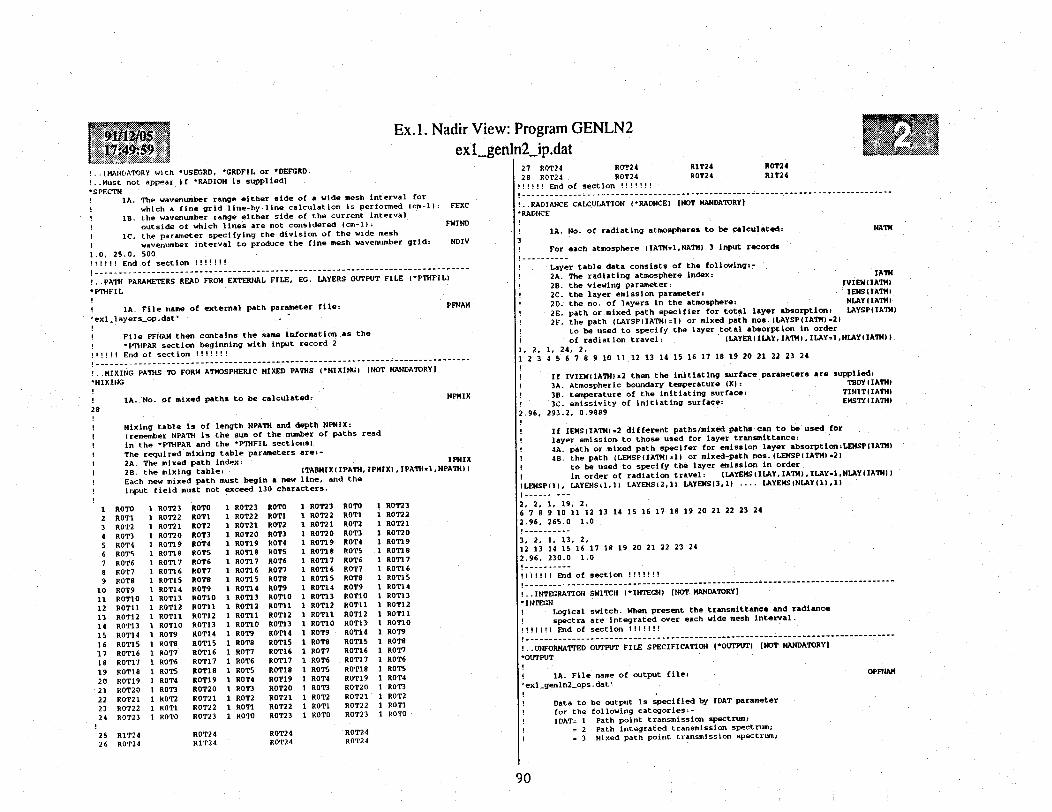
Ex. 1. Nadir'exl

!..(MANDATORY with *USEGRD, *GRDFIL or *DEFGRD.

!..Must not appear if *RADIOM is supplied)*SPECTM

1A. The wavenumber range either side of a wide mesh interval for

* which a fine grid line-by-line calculation is performed (cm-1): FEXC

! B. the wavenumber range either side of the current interval

! outside of which lines are not considered (cm-l): FWIND

1C. the parameter specifying the division of the wide mesh

, wavenumber interval to produce the fine mesh wavenumber grid: NDIV

1.0, 25.0, 500! I!!! End of section ! !!!!!

!--------------------------------------

!..PATH PARAMETERS READ FROM EXTERNAL FILE, EG. LAYERS OUTPUT FILE (*PTHFIL)

*PTHFIL

1A. File name of external path parameter file: PFNAM

'exl_layers_op.dat'

! File PFNAM then contains the same information as the

! PTHPAR section beginning with input record 2

!1!!!! End of section !!!!!!

!..MIXING PATHS 'D FORM ATMOSPHERIC MIXED PATHS (*MIXING} INOT MANDATORYI

*MIXING

1A. No. of mixed paths to be calculated: NPMIX

28

Mixing table is of length NPATH and depth NPMIX:

i remember NPATH is the sum of the number of paths read

in the *PTHPAR and the *PTHFIL sections)

The required mixing table parameters are:-

2A. The mixed path index: IPMIX

2B. the mixing table: (TABMIX(IPATH,IPMIX),IPATH=I,NPATH))

Each new mixed path must begin a new line, and the

input field must not exceed 130 characters.

123456789

101112131415161718192021222324

ROTOROT1ROT2ROT3ROT4ROT5ROT6ROT7ROT8ROT9ROT10ROTI1ROT12ROT13ROT14ROT15ROT16ROT17ROT18ROT19ROT20ROT21ROT22ROT23

1 ROT231 ROT221 ROT211 ROT201 ROT191 ROT181 ROT171 ROT161 ROT151 ROT141 ROT131 ROT121 ROT111 ROT101 ROT91 ROT81 ROT71 ROT61 ROT51 ROT41 ROT31 ROT21 ROT11 ROTO

25 R1T2426 ROT24

ROTOROT1ROT2ROT3ROT4ROT5ROT6ROT7ROT8ROT9ROT10ROT1ROT12ROT13ROT14ROT15ROT16ROT17ROT18ROT19ROT20ROT21ROT22ROT23

ROT24R1T24

1 ROT231 ROT221 ROT211 ROT201 ROT191 ROT181 ROT171 ROT161 ROT11 ROT141 ROT131 ROT121 ROT111 ROT101 ROT91 ROT81 ROT71 ROT61 ROT51 ROT41 ROT31 ROT21 ROT11 ROTO

ROTOROT1ROT2ROT3ROT4ROTSROT6ROT7ROT8ROT9ROT10ROT1ROT12ROT13ROT14ROT1SROT16ROT17ROT18ROT19ROT20ROT21ROT22ROT23

ROT24ROT24

1 ROT231 ROT221 ROT211 ROT201 ROT191 ROT181 ROT171 ROT161 ROT151 ROT141 ROT131 ROT121 ROT11 ROT101 ROT91 ROT81 ROT71 ROT6I ROTS1 ROT41 ROT31 ROT21 ROT11 ROTO

ROTOROT1ROT2ROT3ROT4ROT5ROT6ROT7ROT8ROT9ROT10ROT1ROT12ROT13ROT14ROT 5ROT16ROT17ROT18ROT19ROT20ROT21ROT22ROT23

ROT24ROT24

1 ROT231 ROT221 ROT211 ROT201 ROT191 ROT181 ROT171 ROT161 ROT151 ROT141 ROT131 ROT121 ROT111 ROT101 ROT91 ROT81 ROT71 ROT61 ROT51 ROT41 ROT31 ROT21 ROT11 ROTO

View: Program GENLN2[_genln2_ip.dat

2? R0T24 R0T24 R1T24 R0T2427 ROT24 ROT24 R1T24 ROT24

28 ROT24 ROT24 ROT24 R1T24i!!! End of section i!!!!!!

.. RADIANCE CALCULATIOI (*RADNCE) (NOT MANDATORY)RADICE

1A. No. of radiating atmospheres to be calculated:

For each atmosphere (IATM=1,NATM) 3 input records

Layer table data consists of the following:-2A. The radiating atmosphere index: IATH

2B. the viewing parameter: IVIEWIIATM»

2C. the layer emission parameter: IEMS(IATM)

2D. the no. of layers in the atmosphere: NLAYIIATMI

2E. path or mixed path specifier for total layer absorption: LAYSP(IATM)

2F. the path (LAYSP(IATM)=1) or mixed path nos. LAYSP(IATM-.2)

to be used to specify the layer total absorption in order

of radiation travel: (LAYER(ILAY,IATM),ILAYI1,NLAY(IATM))

1, 2, 1, 24, 2,23 4 5 6 7 8 9 10 11 12 13 14 15 16 17 18 19 20 21 22 23 24

If IVIEW(IATM)=2 then the initiating surface parameters are supplied:

! 3A. Atmospheric boundary temperature (K): TBDYIIATM)

! 3B. temperature of the initiating surface: TINIT(IATH)

! 3C. emissivity of initiating surface: EMSTY(IATM)

2.96, 293.2, 0.9889

! If IEMS(IATM)=2 different paths/mixed paths can to be used for

! layer emission to those used for layer transmittance:

4A. path or mixed path specifer for emission layer absorption:LEMSP(IATM)

! 4. the path (LEMSP(IATM)=1) or mixed-path nos.(LEMSP(IATM)-2)to be used to specify the layer emission in order

in order of radiation travel: (LAYEMS(ILAY,IATM),ILAY=1,NLAY(IATH))

!LEMSP(l), LAYEMSl,1) LAYEMSI2,1 ) LAYEMS(3,1 .... LAYEMS31LAY(l),I)I.---------

2, 2, 1, 19, 2,6 7 8 9 10 11 12 13 14 15 16 17 18 19 20 21 22 23 24

2.96, 265.0 1.0I---------3, 2, 1, 13, 2,12 13 14 15 16 17 18 19 20 21 22 23 24

2.96, 230.0 1.0!----------!!!!!!! End of section !!!!!!

!.. ITEGRATION SWITCH (*INTEG;) (NOT MANDATORYI*INTEGN! Logical switch. When present the transmittance and radiance

! spectra are integrated over each wide mesh interval.

!!!!! ! End of section i !!!!!!---------------------------------__-------------------__---____________________!..UNFORMATTED OUTPUT FILE SPECIFICATION (*OUTPUT) (NOT MANDATORY)

*OUTPUT

1IA. File name of output file: OPFNAM

'exl_genln2_ops.dat'

, Data to be output is specified by IDAT parameter

! for the following categories:-IDAT= 1 Path point transmission spectrum;

! = 2 Path integrated transmission spectrum;! = 3 Mixed path point transmission spectrum;

90

3

INATI

I

! = 4 Mixed path integrated transmission spectrum;! · S Layer point transmission spectrum;

! 6 Layer integrated transmission spectrum;! = 7 Layer point radiance spectrum;* = 8 Layer integrated radiance spectrum.

The following section is repeated for each required IDAT.

2A. Index (1 thro' 8 above):3

For IDAT = 1, 2, 3 or 4:3A. no. of paths or mixed paths to be output:

! if all paths are to be printed set NP<0.For IDAT = 5, 6, 7 or 8:

! 3A. atmosphere no. for output:! if all atmospheres are to be output set IATM<0.

3B. no. of layers to be output:! if all layers are to be output set NP<0.

.---.. 3'-

IDAT

NP

IATM

NP

4

For all IDAT:! 4A. List of path, mixed path or layer nos. for output;

! only required if NP>0; (IOPGR(IDAT,IATM,I,.I=1,NP)25 26 27 28

71, 124!----------72, 119!----------73, 113

81, 124!----------82. 119

83, 113!----------i!!!!! End of section !!!!I!!!---------------------------------------------------------_

!..END OF GENLN2 INPUT (*ENDINP) (MANDATORY]*ENDINP!!!!!!! End of input data to GENLN2 !!!!!!

Ex. 1. Nadir View: Program GENLN2exl eenln2 intdat

91

--- - IroA-AW

Ex. 1. Nadir View: Program GENGRP

: : .:S .:: ::::: ::::::. :::: -: : : . : . . . : ._.. ... - : r ....... I .. ... :**********************************************

************************************************

** GENLN2: GENERAL LINE-BY-LINE ATMOSPHERIC **** TRANSMITTANCE AND RADIANCE MODEL **** VERSION 3.0 D.P. EDWARDS 27/02/91 **** (C) COPYRIGHT 1991 UCAR/NCAR **** ALL RIGHTS RESERVED **** GENLN2 SOFTWARE AND RELATED MATERIALS **

** MAY BE USED ONLY UNDER AN EXECUTED VALID **** LICENCE AGREEMENT ***************************************************

***************************** * ****************** *

DATE (DAY.MON.YR): 20.12.91

*************** CHECK INPUT DATA FOR ERRORS ***************

*************** INPUT DATA SUCCESSFULLY READ *************

*************** SUMMARY OF INPUT DATA *************

TITLE OF THIS RUN :- Nadir example calculation: AVHRR Ch.4

LINE AND CROSS-SECTION DATA*****************************

1 LINE DATA FILE(S) WILL BE USED

FILE NO. 1 FILENAME exl_hitlin_op.dat3 GAS(ES) TO BE READ, MOLEC ID NO(S):- 1 2 3

GAS LINE VERSION(S) TO BE CHOSEN:- 10 10 10

1 XSEC DATA FILE(S) WILL BE USEDFILE NO. 1 FILENAME xsec.dat

1 XSEC(S) TO BE READ, MOLEC ID NO(S):- 52

!II I ! I I I I I I I I I I I -l I I I II111 1l I t1 1 1 l I I I I I I ! I 11 1 ! I I 1 1 11 l l I I I 11l I l l I 1 l l l l l l l I 1 1 I l l l l l 1

WAVENUMBER GRID

TOTAL WAVENUMBER RANGE CONSIDERED 825.000 - 1025.000 cm-1

PASSBAND (INTEGRATION) WAVENUMBER RANGE 850.000 - 1000.000 cm-1

THIS CONSISTS OF 150 INTERVALS OF AVERAGE WAVENUMBER WIDTH 1.000 cm-1

EACH INTERVAL WILL BE DIVIDED INTO 500 FINE MESHES FOR THE TRANSMITTANCE CALCULATION.

TRANSMITTANCE CALCULATION***************************

THE LINE ABSORPTION IN A RANGE OF 1.000 cm-1 EITHER SIDE OF THE WIDEMESH INTERVAL WILL BE TREATED EXPLICITLY.

THE WING ABSORPTION DUE TO LINES LYING IN THE RANGE 1.000 - 25.000 cm-1

EITHER SIDE OF THE WIDEMESH INTERVAL WILL BE INCLUDED.

THE CONTINUUM ABSORPTION WILL BE INCLUDED FOR APPROPRIATE PATHS.

1l!!1 !lllllll ! l1llll1!1 1 1111 !lllllllllllllllllll!lllll 1l1!ll 11111111111I1111I111I

92

Ex.1. Nadir View: Program GENGRP..i ex|geln .. pd..dat.. .::.- :: . * . :* * :: ........ ............ ........ . :. . ..... .... ... ....... ...... . .......Iliil~iliii:::i: I i

PATH DATA*********

PATH FILE GAS ID ISO ID AMT kg.moles/cm2 T K P atm PARTP atm VEL m/s LINESHAPE CONTINUUM

1 1 1 0 6.951E-05 291.911 9.431E-01 1.562E-02 0.000E+00 VOIGT CON

2 1 1 0 4.313E-05 286.966 8.298E-01 9.640E-03 0.000E+00 VOIGT CON

3 1 1 0 2.086E-05 281.543 7.352E-01 5.721E-03 0.000E+00 VOIGT CON

4 1 1 0 1.251E-05 276.124 6.583E-01 3.333E-03 0.000E+00 VOIGT CON

etc.

93 1 52 0 6.652E-18 272.120 1.343E-03 3.115E-16 0.000E+00 XSECTION NOCON

94 1 52 0 3.324E-26 247.872 1.962E-04 1.962E-24 0.000E+00 XSECTION NOCON

95 1 52 0 5.769E-27 230.602 1.047E-04 1.047E-24 0.000E+00 XSECTION NOCON

96 1 52 0 1.308E-30 205.677 3.030E-05 3.030E-29 0.000E+00 XSECTION NOCON

11111 |1 l111i lii ~11111 1!! -11111111 ilt1 !11 III I iI II 11i i i !1111 1

l111it lI tl 1 1ti 11111 Il It

MIXING TABLE DATA***** ************

MIXING TABLE IS OF LENGTH 96 PATH(S) AND DEPTH 28 MIXED PATH(S)

I I I I I I III IIIIII 1 ! 11 I I I I I I I I I I I I I I I I I I II I I I I I I I I I I I I I I I 1I I I I I I I I I I I I I I I I I I I 1 1 1 1 1 1 1 1 1 1 1 1 1 1 11 1 1 i 1 1 1 1 1 1 111 1 11 1

RADIANCE DATA

CALCULATIONS WILL BE PERFORMED FOR 3 RADIATING ATMOSPHERE(S)

ATMOSPHERE NO LAY PTHMIX PATH/MIX ED PATH NOS TO BE USED FOR LAYER TRANSMITTANCE IN ORDER OF THE DIRECTION OF RADIATION TRAVEL

1 24 2 1 2 3 4 5 6 7 8 9 10 11 12 13 14 15 16 17 18 19 20 21 22 23 24

VIEWING PARAMETER = 2 ATMOSPHERIC BOUNDARY TEMP. (K) = 2.960 SURFACE EMITTANCE = .98890 SURFACE TEMP. (K) = 293.200

2 19 2 6 7 8 9 10 11 12 13 14 15 16 17 18 19 20 21 22 23 24

VIEWING PARAMETER = 2 ATMOSPHERIC BOUNDARY TEMP. (K) = 2.960 SURFACE EMITTANCE = 1.00000 SURFACE TEMP. (K) = 265.000

3 13 2 12 13 14 15 16 17 18 19 20 21 22 23 24

VIEWING PARAMETER = 2 ATMOSPHERIC BOUNDARY TEMP. (K) = 2.960 SURFACE EMITTANCE = 1.00000 SURFACE TEMP. (K) = 230.000

SPECTRA WILL BE INTEGRATED OVER THE WIDEMESH INTERVALS.

I I I I I I I I I I I I I I I I I I I I I I I I I I I I I I I I I I I I I I I I I I I I I I I I I I I I I I I I I I I I I I I I I I I I I I I I I I I I I I ! I I I I I I I I I I I I 1 1 1 1 1 1 1 1 1 1 1 I I I i 1 1 1 1 1 1 1 1 1 1 1 1 1 1 1 1 1 1 1 1

+************** CALCULATION BEGINS **********

*************** ELAPSED CPU TIME: 2:17:38.13 ***************

****** ****** CALCULATION COMPLETE. ********

1If1 Illllil11ll lll11 lllll ll l! I ll l 1l SlllllllI Illl!l ll lllllll i l llllllllllll.ll I!!!! !lll IIII

INTEGRATED MIXED PATH TRANSMITTANCES************ ******************

*** MIXED PATH NO. 25 **

93

1. Nadir View: Program GENGFilexl: genl ̂ ::d

. ... .... .. .. .. .....

INTERVAL LOW BDY cm-1 UPP BDY cm-1 FINE MESHES TRANSMITTANCE

1 850.000 851.000 500 .359862E+00

2 851.000 852.000 500 .660303E+00

3 852.000 853.000 500 .603862E+00

etc.

148 997.000 998.000 500 .818423E+00

149 998.000 999.000 500 .810427E+00

150 999.000 1000.000 500 .719268E+00

AVERAGE VALUE OVER PASSBAND .714597E+00

*** MIXED PATH NO. 26 ***INTERVAL LOW BDY cm-1 UPP BDY cm-1 FINE MESHES TRANSMITTANCE

1 850.000 851.000 500 .999121E+00

2 851.000 852.000 500 .999402E+00

3 852.000 853.000 500 .999660E+00

etc.

148 997.000 998.000 500 .999132E+00

149 998.000 999.000 500 .999743E+00

150 999.000 1000.000 500 .999131E+00

AVERAGE VALUE OVER PASSBAND .986363E+00

*** MIXED PATH NO. 27 ***INTERVAL LOW BDY cm-1 UPP BDY cm-1 FINE MESHES TRANSMITTANCE

.1 850..000 851.000 500 ...........99 ...9963E+....00

2 851.000 852.000 500 .999963E+002 851.000 852.000 500 .999950E+00

3 852.000 853.000 500 .999977E+00

etc.

148 997.000 998.000 500 .914000E+00

149 998.000 999.000 500 .871733E+00

150 999.000 1000.000 500 .870319E+00

AVERAGE VALUE OVER PASSBAND .991805E+00

*** MIXED PATH NO. 28 ***INTERVAL LOW BDY cm-1 UPP BDY cm-1 FINE MESHES TRANSMITTANCE

1 850.000 851.000 500 .10000.....0......E+..01

2 851.000 851.000 500 .100000E+012 851.000 852.000 500 .100000E+013 852.000 853.000 500 .100000E+01

etc.

148 997.000 998.000 500 .100000E+01

149 998.000 999.000 500 .100000E+01

150 999.000 1000.000 500 .100000E+01

AVERAGE VALUE OVER PASSBAND .995772E+00

INTEGRATED ATMOSPHERIC LAYER TRANSMITTANCES AND BOUNDARY RADIANCES****************************** ***** *

*** ATMOSPHERE 1 ***

94

--------------------

i: tr.·. · .X ·· ·. ···. .. .. ...... . ... . ...

Ex.1. Nadir View: Program G:. ie:in2:. :;1: l i .. .f:d: dnl2 d at

.. .f . .... ... . ... ....; ... . . . . _ . . ..... ......:-:::::--·: ---- ·-- : · · : ex~nl~a~at

*** LAYER NO. 24 ***INTERVAL LOW BDY cm-1 UPP BDY cm-1 FINE MESHES TRANSMITTANCE BDY RADIANCE

W/(m2.sr.cm-1)

1 850.000 851.000 500 .359468E+00 .103922E+002 851.000 852.000 500 .659876E+00 .110991E+00

3 852.000 853.000 500 .603635E+00 .110248E+00

etc.

147 996.000 997.000148 997.000 998.000149 998.000 999.000150 999.000 1000.000

AVERAGE VALUES OVER PASSBAND

500500500500

.721097E+00

.747411E+00

.705887E+00

.623999E+00

.694896E+00

.809996E-01

.823899E-01

.797261E-01

.786304E-01

.975753E-01

*** ATMOSPHERE 2 ***

*** LAYER NO. 19 ***INTERVAL LOW BDY cm-1 UPP BDY cm-1 FINE MESHES TRANSMITTANCE BDY RADIANCE

W/(m2.sr.cm-1)

1 850.000 851.000 500 .931149E+00 .725256E-01

2 851.000 852.000 500 .994890E+00 .729145E-013 852.000 853.000 500 .992876E+00 .727609E-01

etc.

148 997.000 998.000149 998.000 -39.000150 999.000 1000.000

AVERAGE VALUES OVER PASSBAND

500500500

.919950E+00

.879940E+00

.874501E+00

.977949E+00

.507644E-01

.495883E-01

.494062E-01

.622611E-01

*** ATMOSPHERE 3 ***

*** LAYER NO. 13 ***INTERVAL LOW BDY cm-1 UPP BDY cm-1 FINE MESHES TRANSMITTANCE BDY RADIANCE

W/(m2.sr.cm-l)

1 850.000 851.000 500 .999057E+00 .360143E-01

2 851.000 852.000 500 .999915E+00 .359162E-013 852.000 853.000 500 .999934E+00 .358169E-01

148149150

AVERAGE VALUES

997.000 998.000998.000 999.000999.000 1000.000OVER PASSBAND

500500500

.930116E+00

.892822E+00

.892637E+00

.991183E+00

.232589E-01

.232763E-01

.231814E-01

.291857E-01

*************** END OF DATA OUTPUT ***************

*************** GRAPHICS FILE WRITTEN TO: exl_genln2_ops.dat

95

IIIIIII IIIIIIII11111t1111 '1111111111111-

I| PROGRAM GENGRP IIII _II------- -|

II GENERAL PURPOSE GRAPHICS FOR PLOTTING IIII GENLN2 TRANSMITTANCE AND RADIANCE SPECTRA II

II VERSION 3.0 D.P. EDWARDS 27/02/91 II

II (C) COPYRIGHT 1991 UCAR/NCAR IIII ALL RIGHTS RESERVED IIII GENLN2 SOFTWARE AND RELATED MATERIALS MAY 11II BE USED ONLY UNDER AN EXECUTED VALID II

II LICENCE AGREEMENT II1111111111111111111111111111 1111111ffiI

II ""I"IIIl I"it1111111111111111 1.111111111.1111111

**Q** Name of GENLN2 unformatted output-'file to plot? :

ex1 _genln2_ops dat**Q** Enter filename of output graphics metacode file:

exlgengrp_trans .meta**Q** Do you want the default picture size (Y/NI

Y**Q** For a default axis, the axis drawn will be

that appropriate for the first curve entered.Is a default X-axis to be drawn? (Y/N) :

Y**Q** Is a default Y-axis to be drawn? (Y/N :

Y**Q** Enter the no. of curves to be plotted on this graph? :

4**Q* Do you want to supply your own curve captions? [Y/N) :

Y1101 CURVE 1O. 1 11111**Q** Is a path transmittance spectrum (PT),

a mixed path transmittance spectrum (XT),

a radiating atmosphere layer transmittance spectrum (AT),

or a radiating atmosphere layer radiance spectrum (AR)

to be plotted?Enter one of PT, XT, AT or AR:

XT**Q** Curve 1. IPMIX no. of mixed path to be plotted?

25**Q** Are wide mesh binned spectral values to be plotted? [Y/N)

N**Q** Enter line type and pen type for drawing curve LTYPE,IPEN

1,2**Q** Enter curve caption, 50 chars. max.:H20 transmittance111 CURVE NO. 2 11111**Q** Is a path transmittance spectrum (PT),

a mixed path transmittance spectrum (XT),

a radiating atmosphere layer transmittance spectrum (AT),

or a radiating atmosphere layer radiance spectrum (AR)

to be plotted?Enter one of PT, XT, AT or AR:

XT**Q** Curve 2. IPMIX no. of mixed path to be plotted?

26**Q** Are wide mesh binned spectral values to be plotted? (Y/N]

N**Q** Enter line type and pen type for drawing curve LTYPE,IPEN

1,3**Q** Enter curve caption, 50 chars. max.:

Ex.1. Nadir View: Program GENGRP.exlgengr trans.dat' ' : 'I: :

C02 transmittance1IIII CURVE NO. 3 1111**Q** Is a path transmittance spectrum (PT),

a mixed path transmittance spectrum (XT),a radiating atmosphere layer transmittance spectrum (AT),

or a radiating atmosphere layer radiance spectrum (AR)

to be plotted?Enter one of PT, XT, AT or AR

XT*'Q** Curve 3. IPMIX no. of mixed path to be plotted?27**Q** Are wide mesh binned spectral values to be plotted? [Y/N :

N**Q** Enter line type and pen type for drawing curve LTYPE,IPEN :

1,4**Q** Enter curve caption, 50 chars. max. ,03 transmittance11111 CURVE NO. 4 11111**Q* Is a path transmittance spectrum (PT),

a mixed path transmittance spectrum (XT),a radiating atmosphere layer transmittance spectrum (AT),

or a radiating atmosphere layer radiance spectrum (AR)

to be plotted?Enter one of PT, XT, AT or AR:

XT**Q** Curve 4. IPMIX no. of mixed path to be plotted?

28**Q** Are wide mesh binned spectral values to be plotted? (Y/IN)

N**Q** Enter line type and pen type for drawing curve LTYPE,IPEN :

1,5»*Q** Enter curve caption, 50 chars. max.CFC12 transmittance**Q** Do you want to degrade the spectra with an

instrument line shape (ILS) function? (Y/NI :Y**Q** ILS function type specifier;

1 square boxcar2 = triangle3 = Fourier spec. (only with evenly spaced points)4 , user supplied (only with evenly spaced points)Enter 1,2,3 or 4

2~: *~'*Q** Enter triangle half power band width in cm-1 i0.5

l~: '~**Q** Are all points to be plotted? Y/N):N**Q** Enter no of plot points/cm-:50*'Q** Is an external spectra to be plotted? (Y/N] iY**Q** Enter number of external spectra for plotting111111 EXTERNAL SPECTRUM NO. 1 110ll**Q** Enter name of file containing spectrum dataex l_gengrp_res .dat**Q** Enter line type and pen type for drawing curve LTYPE,IPEN :

2,1**Q** Enter spectrum caption, 50 chars. max. :

1~~~: ~ AVHRR Channel 4**Q** Enter spectrum plot Y-axis title:

I : RADIOMETER RESPONSE

96

GENLN2, TRANSMITTANCE SPECTRUM

860 880 900 920 940 960 980 1000

WAVENUMBER cm-1

Nadir example calculation: AVHRR Ch.4H20 transmittanceC02 transmittance03 transm ttanceCF'C12 transm ttance

------- AVHRR Channel 4

97

1.0

.9

.8

.7

wL.)z

t-

2,

zcc

.6

.5

.4

wtnz0U,

Ix

0

c0c

.3

.2

.1

0

III IIIIIUIIIIIIIIIIIIIIIIIII IIIIIIIII1 INBIit l I II IIIIIiimIII iiiIII II I Ii ii ii iI

I PROGRAM GENGRP IIII IIII GENERAL PURPOSE GRAPHICS FOR PLOTTING II1I GENLN2 TRANSMITTANCE AND RADIANCE SPECTRA IIII VERSION 3.0 D.P. EDWARDS 27/02/91 11II (C) COPYRIGHT 1991 UCAR/NCAR I1II ALL RIGHTS RESERVED IIII GENLN2 SOFTWARE AND RELATED MATERIALS MAY IIII BE USED ONLY UNDER AN EXECUTED VALID IIII LICENCE AGREEMENT II11"§1111Illlllllllllllllllllll Illlllllllllllll

I11111111I1 111II 11III IIII 111 1111111I1tll lIIIII

** N* Name of GENLN2 unformatted output file to plot? :exl_genln2_ops.dat**Q** Enter filename of output graphics metacode file :ex _gengrp_cfc12 met a**Q*' Do you want the default picture size [Y/N:Y**Q** For a default axis, the axis drawn will be

that appropriate for the first curve entered.Is a default X-axis to be drawn? (Y/N :

**Q* Is a default Y-axis to be drawn? (Y/N :N**Q** Enter XMIN and XMAX values for user's X axis :900.0, 940.0**Q** Enter X axis title:WAVENUMBER cm-1**Q* Are normalized spectra to be plotted? (Y/N]N**Q** Enter YMIN and YMAX values for user's Y axis :0.95, 1.0**Q** Enter 1 for linear scale, 2 for log scale:1**Q** Enter Y axis title:TRANSM I TTANCE

*Q** Enter graph title:GENLN2: TRANSMITTAINCE**Q** Enter the no. of curves to be plotted on this graph? :

1**Q** Do you want to supply your own curve captions? IY/N]Y!111 CURVE NO. 1 III!**Q** Is a path transmittance spectrum (PT),

a mixed path transmittance spectrum (XT),a radiating atmosphere layer transmittance spectrum (AT),or a radiating atmosphere layer radiance spectrum (AR)to be plotted?Enter one of PT, XT, AT or AR:

XT**Q** Curve 1. IPMIX no. of mixed path to be plotted? :

28**Q** Are wide mesh binned spectral values to be plotted? (Y/N)N**Q** Enter line type and pen type for drawing curve LTYPE, IPEN :1,5**Q** Enter curve caption, 50 chars. max.

.x.l. Nadir View: Program GENGRPexl_gengrp_cfcl2.dat .t : : .7: :::7 :!.. I . . .... ..

CFC12 transmittance**Q** Do you want to degrade the spectra with an

instrument line shape (ILS) function? (Y/IN)Y*Q** ILS function type specifier;

1 = square boxcar2 a triangle3 = Fourier spec. (only with evenly spaced points)4 = user supplied (only with evenly spaced points)Enter 1,2,3 or 4

2**Q** Enter triangle half power band width in cm-10.5**Q** Are all points to be plotted? (Y/N]N**Q** Enter no of plot points/cm-150**Q** Is an external spectra to be plotted? Y/N):N

98

i

GENLN2, TRANSMITTANCE

f1TU1- I rrjJ r1SrrIrlrrr r rrlrtf]ut E~jI~ I I I I jIruIl

910 915 920 925 930WAVENUMBER cm-1

Nadir examole calculationt AVHRR Ch.4

935

I CFC12 transmittanceb·~~~~~~~~~~~~~~~~~~~~~~~~~~~~~~~~~~~~~~~~~~,

99

1.101

.995

.991

.985

.989

9uz

9CI.975.

2

2U)

.971

.965

.968

.955

1.000

.995

.990

.985

.980

.975

.970

.965

.960

.955

.950900 905

. . a. . . . . . . . . . . . .... . . . . . . . . . . . . . . . . . . . . ..a. . .e.i. .a I I .a a a u.. . . . . .

940

I I I I I I I I I I I I I I I 9 I I I I I I I I I I I lln I I I I

E

E

to . .III11 11 IIII111)111)1

11111)11~~~~~~~~~11111111~~~~~~~~11()(111( ~ ~ ~ ~ ~ ~ ~ ~ ~ ~ ~ 1

I

Irlllcclllrltll��r 1rlllIlrl-ltlloca

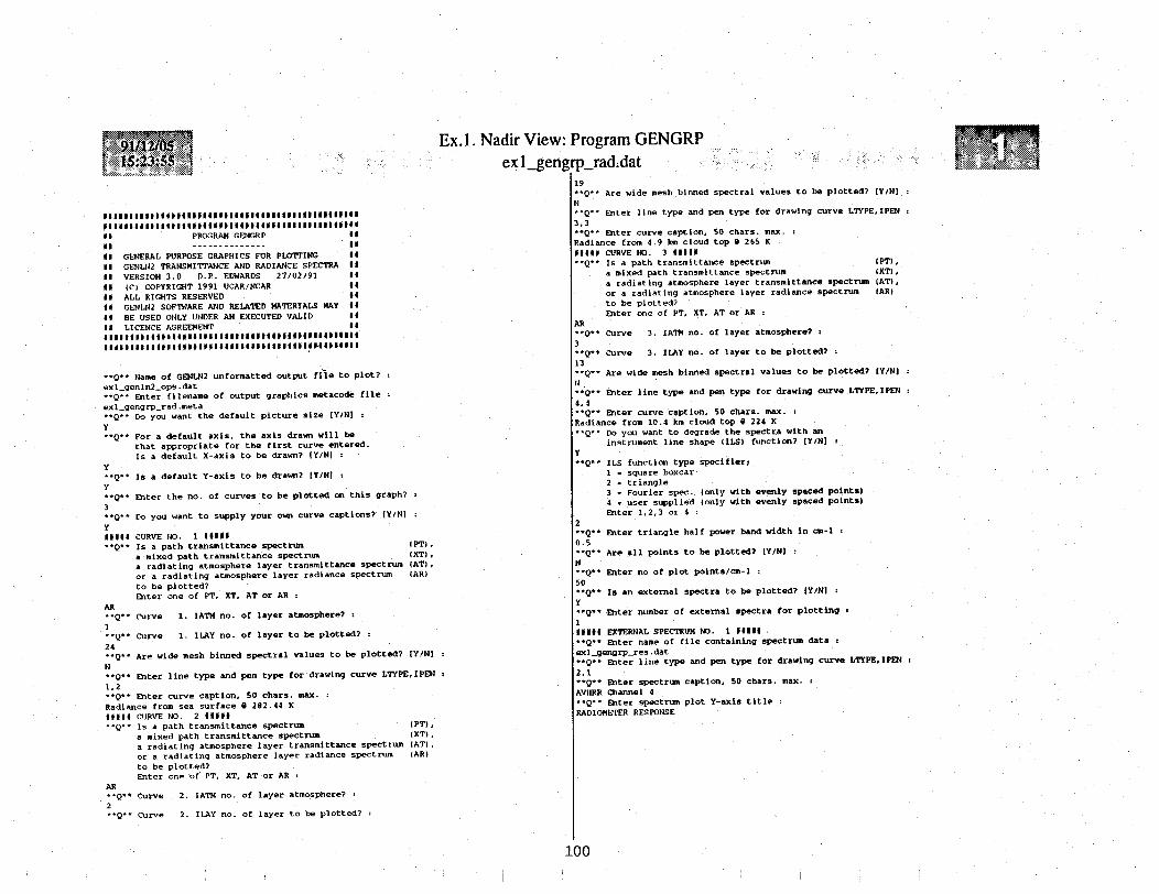
Ex.1. Nadir View: Program GENGRPexigengrprad.dat_.- e da . .

IIIIII11II11II 1111111 1I1I11111II111111I11

II PROGRAM GENGRP I1

II --------- I-II GENERAL PURPOSE GRAPHICS FOR PLOTTING II11 GE4NLN2 TRANSMITTANCE AND RADIANCE SPECTRA 11II VERSION 3.0 D.P. EDWARDS 27/02/91 1III (C) COPYRIGHT 1991 UCAR/NCAR IIII ALL RIGHTS RESERVED II

II GENLN2 SOFTWARE AND RELATED MATERIALS MAY II

II BE USED ONLY UNDER AN EXECUTED VALID IIII LICENCE AGREEMENT II

II 1111)1 II 1III)II1 11113111 111111111111111

OQ** Name of GENLN2 unformatted output file to plot? :

exl_genln2_ops. dat**Q** Enter filename of output graphics metacode file :

exl_gengrp_rad .meta**Q** Do you want the default picture size [Y/NIY**Q** For a default axis, the axis drawn will be

that appropriate for the first curve entered.Is a default X-axis to be drawn? (Y/N :

Y**Q** Is a default Y-axis to be drawn? (Y/N :Y**Q** Enter the no. of curves to be plotted on this graph? :

3**Q** Do you want to supply your own curve captions? (Y/N :

Y1111 CURVE O10. 1 11111**Q** Is a path transmittance spectrum (PT),

a mixed path transmittance spectrum (XT),a radiating atmosphere layer transmittance spectrum (AT),

or a radiating atmosphere layer radiance spectrum (AR)

to be plotted?Enter one of PT, XT, AT or AR:

AR**Q** Curve 1. IATH no. of layer atmosphere? :

1**Q** Curve 1. ILAY no. of layer to be plotted?:

24**Q** Are wide mesh binned spectral values to be plotted? (Y/N:

N**Q** Enter line type and pen type for drawing curve LTYPE,IPEN:

1,2**Q** Enter curve caption, 50 chars. max. :

Radiance from sea surface B 282.44 K1111 CURVE NO. 2 11111**Q* Is a path transmittance spectrum (PT),

a mixed path transmittance spectrum (XT),

a radiating atmosphere layer transmittance spectrum (AT),

or a radiating atmosphere layer radiance spectrum (AR)

to be plotted?Enter one of PT, XT, AT or AR

AR**Q** Curve 2. IATM no. of layer atmosphere?2**Q** Curve 2. ILAY no. of layer to be plotted?:

19**Q** Are wide mesh binned spectral values to be plotted? (Y/N]H**Q** Enter line type and pen type for drawing curve LTYPE,IPEN :

3,3**Q** Enter curve caption, 50 chars. max. :Radiance from 4.9 km cloud top 0 265 K11ll1 CURVE TO. 3 11111**Q** Is a path transmittance spectrum (PT),

a mixed path transmittance spectrum (XT),

a radiating atmosphere layer transmittance spectrum (AT),

or a radiating atmosphere layer radiance spectrum (AR)

to be plotted?Enter one of PT, XT, AT or AR:

AR**Q** Curve 3. IATM no. of layer atmosphere? :

3*Q** Curve 3. ILAY no. of layer to be plotted? :

13**Q** Are wide mesh binned spectral values to be plotted? (Y/N:

N**Q** Enter line type and pen type for drawing curve LTYPE,IPEN:

4,4**Q** Enter curve caption, 50 chars. max.Radiance from 10.4 km cloud top Q 224 K**Q** Do you want to degrade the spectra with an

instrument line shape (ILS) function? (Y/N] :Y**Q** ILS function type specifier;

1 = square boxcar2 = triangle3 = Fourier spec. (only with evenly spaced points)4 = user supplied (only with evenly spaced points)Enter 1,2,3 or 4

2**Q** Enter triangle half power band width in cm-l

0.5**Q** Are all points to be plotted? (Y/N :N**** Enter no of plot points/cm-l50**Q** Is an external spectra to be plotted? (Y/N:Y**Q** Enter number of external spectra for plotting :111111 EXTERNAL SPECTRUM NO. 1 11 11**Q** Enter name of file containing spectrum data:exl_gengrpres.dat**Q** Enter line type and pen type for drawing curve LTYPE,IPEN:

2,1**Q** Enter spectrum caption, 50 chars. max.AVHRR Channel 4**Q** Enter spectrum plot Y-axis title:RADIOMETER RESPONSE

100

T

GENLN2. RADIANCE SPECTRUM

_I.~~~~~ ~ ~~~ _-~~~~ ~ ~~~~~~ _-~~ _- " \ . -].013

E -\

h ~_ _ /-. 007

- /_ I -.es: . t -_

' r I _\-- I i^.

I

_ 0 \ _~._~~~~~~~~~~~~~~~~~~~~~~.003

-~: I/~ \

_ /_

- I L I I I , I I I I II I I -I I 1.0

860 80 900 920 940 960 980 1000

WAVENUMBER cm-1

Nadir example calculation: AVHRR Ch.4Radiance from sea surface · 282.44 K

- - - - - Radiance from 4.9 km cloud top · 265 KRadiance from 10.4 km cloud top 0 224 K

-- ----- -AVHRR Channel 4

101

.12

.11

.10

* .09

L

E .08

wu .07z

-cJ

: .06

-J

.04

.03

.02

2

C

I-

Ln

z

CCw

wwX

ct

cc

I

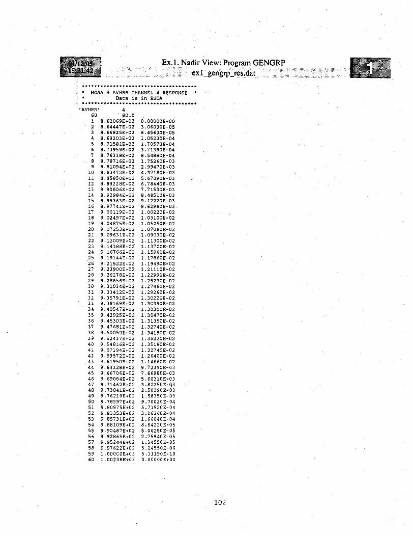
Ex. 1. Nadir View: Program GENGRP;;,:: :::' ;. .. :.:.;.:g s: .: ; ; ... :..... ...

* NOAA 9 AVHRR CHANNEL 4 RESPONSE *! * Data is in ESDA! *************************************

'AVHRR' 460 80.01 8.62069E+02 O.OOOOOE+002 8.64447E+02 3.06030E-053 8.66825E+02 6.45630E-054 8.69203E+02 1.05230E-045 8.71581E+02 1.70570E-046 8.73959E+02 3.71390E-047 8.76338E+02 8.54880E-048 8.78716E+02 1.75260E-039 8.81094E+02 2.99470E-03

10 8.83472E+02 4.37180E-0311 8.85850E+02 5.67390E-0312 8.88228E+02 6.78440E-0313 8.90606E+02 7.71530E-0314 8.92984E+02 8.48510E-0315 8.95363E+02 9.12220E-0316 8.97741E+02 9.62980E-0317 9.00119E+02 1.00220E-0218 9.02497E+02 1.03100E-0219 9.04875E+02 1.05250E-0220 9.07253E+02 1.07080E-0221 9.09631E+02 1.09030E-0222 9.12009E+02 1.11300E-0223 9.14388E+02 1.13700E-0224 9.16766E+02 1.15960E-0225 9.19144E+02 1.17860E-0226 9.21522E+02 1.19490E-0227 9.23900E+02 1.21110E-0228 9.26278E+02 1.22990E-0229 9.28656E+02 1.25230E-0230 9.31034E+02 1.27460E-0231 9.33412E+02 1.29260E-0232 9.35791E+02 1.30220E-0233 9.38169E+02 1.30390E-0234 9.40547E+02 1.30300E-0235 9.42925E+02 1.30470E-0236 9.45303E+02 1.31350E-0237 9.47681E+02 1.32740E-0238 9.50059E+02 1.34190E-0239 9.52437E+02 1.35220E-0240 9.54816E+02 1.35180E-0241 9.57194E+02 1.32740E-0242 9.59572E+02 1.26400E-0243 9.61950E+02 1.14660E-0244 9.64328E+02 9.72390E-0345 9.66706E+02 7.66980E-0346 9.69084E+02 5.60310E-0347 9.71462E+02 3.82250E-Q348 9.73841E+02 2.50390E-0349 9.76219E+02 1.58350E-0350 9.78597E+02 9.70020E-0451 9.80975E+02 5.71920E-0452 9.83353E+02 3.16260E-0453 9.85731E+02 1.66040E-0454 9.88109E+02 8.84220E-0555 9.90487E+02 5.06250E-0556 9.92865E+02 2.75940E-0557 9.95244E+02 1.34550E-0558 9.97622E+02 5.24550E-0659 1.OOOOOE+03 5.31190E-1060 1.00238E+03 0.OOOOOE+00

102

Ex. 1. Nadir View: Program RADTEM.. e::x..;... . ..eX iadtem ip.dat :..... ... . .... . ..... ... .......

Q^ ^# #i##^##^^ ##^^#^^^#^### ### # ###I#Q######### ##########

#*# PROGRAM RADTEM #### ##----------## PROGRAM TO CALCULATE A RADIANCE TO #### EQUIVALENT BRIGHTNESS TEMPERATURE #### LOOK-UP TABLE FOR A GIVEN RADIOMETER #### WIDEBAND RESPONSE FUNCTION. ###1 VERSION 3.0 D.P. EDWARDS 27/02/91 #*### (C) COPYRIGHT 1991 UCAR/NCAR #### ALL RIGHTS RESERVED ##*# GENLN2 SOFTWARE AND RELATED MATERIALS #*## MAY BE USED ONLY UNDER AN EXECUTED #### VALID LICENCE AGREEMENT ##

**Q** Enter name of channel response data file :exl_gengrp_res.dat**Q** Enter name of rad.--> bright.T. output look-up file :exl_radtem_op.dat**Q** Enter the lower and upper temperatures [K] and

no of temperature points per degree K:150.0, 350.0, 10**Q** Enter number of points for spectral integation200

103

Ex.l. Nadir View: Progra: : -. ... .... ... . ... ..... . -. .

............ .. .......::.~: ;:.::.:

....... . . .... . ... .. . ... . - .*.-* ..*...--.-- i

.IIIIIIY IIIIIII~~~~~~~~~~~~~~~~~~~~~..-e

****************************************

** RADTEM: POST-PROCESSING PROGRAM FOR **** GENLN2. RADIANCE-->EQUIVALENT BRIGHTNESS **** TEMPERATURE ((W/(m2.sr.cm-1) ]-->[K]) **** CONVERSION LOOKUP TABLE **** VERSION 3.0 D.P. EDWARDS 27/02/91 **** (C) COPYRIGHT 1991 UCAR/NCAR **** ALL RIGHTS RESERVED **** GENLN2 SOFTWARE AND RELATED MATERIALS **** MAY BE USED ONLY UNDER AN EXECUTED VALID **** LICENCE AGREEMENT **************************************************

************************************************

TEMPERATURES BETWEEN 150.0 AND 350.0 K IN .100 K INTERVALSFILTER PROFILE TAKEN FROM:-

*************************************

* NOAA 9 AVHRR CHANNEL 4 RESPONSE ** Data is in ESDA*************************************

DATA FOR CHANNEL NO. 4FREQUENCY MESH FOR PLANCK FUNCTION CONVOLUTION .705 cm-1.

150.0 350.0 10150.000 1.299550E-03

1.338456E-03151.000 1.378259E-03

1.418973E-03152.000 1.460611E-03

1.503186E-03153.000 1.546712E-03

1.591205E-03154.000 1.636678E-03

1.683143E-03etc.

340.000 1.909020E-011.920293E-01

341.000 1.931601E-011.942942E-01

342.000 1.954319E-011.965730E-01

343.000 1.977175E-011.988655E-01

344.000 2.000170E-012.011718E-01

345.000 2.023301E-012.034919E-01

346.000 2.046570E-012.058256E-01

347.000 2.069975E-012.081731E-01

348.000 2.093518E-012.105342E-01

349.000 2.117198E-012.129088E-01

350.000 2.141013E-012.152972E-01

1.307260E-031.346345E-031.386330E-031.427227E-031.469050E-031.511815E-031.555535E-031.600221E-031.645891E-031.692557E-03

1.911273E-011.922552E-011.933866E-011.945214E-011.956598E-011.968017E-011.979468E-011.990955E-012.002477E-012.014033E-012'.025623E-012.037247E-012.048905E-012.060598E-012.072324E-012.084085E-012.095880E-012.107709E-012.119573E-012.131471E-012.143402E-012.155368E-01

1.315005E-031.354269E-031.394435E-031.435516E-031.477528E-031.520481E-031.564393E-031.609275E-031.655143E-031.702010E-03

1.913526E-011.924812E-011.936134E-011.947489E-011.958879E-011.970304E-011.981763E-011.993257E-012.004784E-012.016347E-012.027944E-012.039575E-012.051241E-012.062940E-012.074674E-012.086441E-012.098244E-012.110080E-012.121950E-012.133854E-012.145793E-012.157765E-01

1.322787E-031.362230E-031.402578E-031.443844E-031.486042E-031.529187E-031.573292E-031.618370E-031.664437E-031.711505E-03

1.915779E-011.927073E-011.938401E-011.949764E-011.961161E-011.972593E-011.984059E-011.995559E-012.007095E-012.018663E-012.030268E-012.041905E-012.053578E-012.065283E-012.077024E-012.088799E-012.100608E-012.112451E-012.124328E-012.136239E-012.148183E-012.160162E-01

1.330603E-031.370226E-031.410756E-031.452208E-031.494594E-031.537930E-031.582229E-031.627503E-031.673769E-031.721039E-03

1.918036E-011.929336E-011.940671E-011.952040E-011.963445E-011.974883E-011.986356E-011.997864E-012.009406E-012.020982E-012.032592E-012.044237E-012.055916E-012.067629E-012.079376E-012.091158E-012.102974E-012.114823E-012.126707E-012.138626E-012.150577E-012.162562E-01

104

I

I

1

I

Ex.1. Nadir View: Program BRIGHT. :. ,, .'. '-":: . .exl'bigh itp. '

######################## ######################################################################### PROGRAM BRIGHT #### --------- ##-## POST-PROCESSING PROGRAM FOR GENLN2: #### CONVOLVES TRANSMITTANCES/RADIANCES WITH #### A RADIOMETER WIDEBAND RESPONSE FUNCTION #### AND OPTIONALLY CONVERTS TO EQUIVALENT #### BRIGHTNESS TEMPERATURE #### VERSION 3.0 D.P. EDWARDS 27/02/91 #### (C) COPYRIGHT 1991 UCAR/NCAR #### ALL RIGHTS RESERVED #### GENLN2 SOFTWARE AND RELATED MATERIALS MAY ### BE USED ONLY UNDER AN EXECUTED VALID #### LICENCE AGREEMENT #### ########*###### #################################################################################

**Q** Enter name of GENLN2 unformatted output file:exl_genln2_ops.dat**Q** Are wide mesh binned spectral values to be used? [Y/N]Y**Q** Enter name of channel response data file :exl_gengrp_res.dat**Q** Are path transmittances to be convolved? [Y/N] :N**Q** Are mixed path transmittances to be convolved? [Y/N] :N**Q** Are layer transmittances to be convolved? [Y/N]N**Q** Are layer radiances to be convolved? [Y/N] :Y**Q** Are brightness temps to be calculated? [Y/N] :Y**Q** Enter name of rad.--> bright.T. look-up file :exl_radtem_op.dat**Q** Enter name of output file :exl_bright_op.dat

105

Ex.1. Nadir View: Program BRIGHT..... x... b.r.igh.o......a..

**.********* ***'*Ww*********** *****WWWWWWWWWW

**************************************************

** BRIGHT: POST-PROCESSING PROGRAM FOR **** GENLN2. CONVOLVES TRANSMITTANCES/RADIANCES **** WITH RADIOMETER WIDEBAND RESPONSE FUNCTION **** AND OPTIONALLY CONVERTS TO EQUIVALENT **** BRIGHTNESS TEMPERATURE **** VERSION 3.0 D.P. EDWARDS 27/02/91 **** (C) COPYRIGHT 1991 UCAR/NCAR **** ALL RIGHTS RESERVED **** GENLN2 SOFTWARE AND RELATED MATERIALS MAY **** BE USED ONLY UNDER AN EXECUTED VALID **** LICENCE AGREEMENT **

GENLN2 OUTPUT DATA FILENAME : exl_genln2_ops.dat

FILTER RESPONSE DATA FILENAME: exl_gengrpres.dat

RADIANCE-->BT TABLE FILENAME : exl_radtem_op.dat

TITLE OF GENLN2 RUN : Nadir example calculation: AVHRR Ch.4

* NOAA 9 AVHRR CHANNEL 4 RESPONSE *! * Data is in ESDA

CONVOLVED LAYER RADIANCES

ATMOSPHERE NO. LAYER NO. CONVOLVED RADIANCE BRIGHTNESS TEMPERATURE[W/(cm-l.sr.m2)] [K]

1 24 9.72727E-02 290.819

2 19 6.17255E-02 264.807

3 13 2.86707E-02 229.983

106

I- - - -- --- - - - - - - - - - - - - - - - - - - - -16 .6 - .6 d

APPENDIX 2. EXAMPLE CALCULATION 2: LIMB VIEW

A2.1 Overview of Example Calculation 2

Example calculation 2 is for a limb viewing geometry problem to reproduce a measure-ment from a high resolution satellite interferometer. The object is to calculate the transmit-tance spectrum for a narrow spectral region near the 720 cm - CO2 Q-branch at a tangentheight of 30 km. An emission calculation is also performed to separate the thermal emissionof C02 and 03.

A2.2 Program HITLIN

Line coupling will be included in this calculation so it is necessary to update the 1991 HI-TRAN database with the line data file, co2mix.dat, that includes the CO2 lines that couple.These lines have the HITRAN REF parameter flagged to indicate that line coupling coeffi-cients exist and will be included in the GENLN2 calculation. The lines from the HITRANfile are given status 10 and those from co2mix.dat are given status 11.

Lines are included over the spectral range 550 to 760 cm-l to cover the CO2 15 Amregion. A binary line data file ex2.hitlin-op.dat for use by GENLN2 is created, with MACH=2since the calculation is performed on the IBM. This file will also be used by the GENLN2PMR calculations of Appendix 3. The input file ex2.hitlinip.dat should be assigned toFORTRAN unit 4 before execution.

A2.3 Program LAYERS

The LAYERS calculation layers the atmosphere using the *MODPRO option and the U.S.1976 Standard atmosphere model profile (MONO=6) from the model atmosphere profile dataset glatm.dat. An integration sub-layer accuracy of 10 is specified and because this is alimb viewing calculation, the refraction calculation is switched on. The lower and upperwavenumbers of the proposed calculation range are provided for use in the calculation of therefractive index of air. The *LEVELS option is used to switch on the printing of a summaryof the layer structure.

The user defined layering option is used and 20 vertical atmospheric layers are definedstarting at the tangent height of 30 km and finishing at 80 km. Notice that a narrow layerstructure is used near the tangent height. A symmetric atmosphere is assumed here, i.e. thesame layers will be used anterior and posterior to the tangent point as shown in Fig.A2.1.Two gases, CO2 and 03 are included in each layer. The C02 line shape with continuum isspecified for use with C02 in the GENLN2 calculation. The Voigt line shape will be usedfor 03. The ray paths are launched from the tangent point at a local zenith angle of 90°and the ray tracing calculation defines curved paths in each concentric layer. The geometryof each path is defined by Fig.3.2 and the angle parameters are output for each path inex2Jayersop.dat.

The input file ex2Jayersip.dat and the output path file ex2Jayers.op.dat shouldbe assigned to FORTRAN units 4 and 30 respectively before execution.

This calculation produces a 20 layer atmosphere with each layer containing 2 gases.There are 40 paths in total, paths 1-20 are for CO2 in layers 1-20, and paths 21-40 are for03 in layers 1-20. The output file, ex2Jayers.op.dat, is used as the input to the *PTHFILinput stage of GENLN2. This file will also be used by the GENLN2 PMR calculations ofAppendix 3.

107

A2.4 Program GENLN2

The line data file produced by HITLIN, ex2_hitlinop.dat, is used when performingthe line-by-line calculation for CO2 and O3. Line coupling is included in the calculation bysetting LCHOSE= 11 for C02 so that the status 11 line parameters, i.e. those lines involved incoupling from file co2mix.dat, are used when they appear on the line file in preference tostatus 10 HITRAN lines. HITRAN status 10 lines are used for O3.

A default, *DEFGRD, wavenumber grid is used and 25 cm- l are allowed for line wingseither side of the pass-band range of 718-722 cm - '. The wide mesh interval DELTA is setat lcm- '. In the *SPECTM section FEXC=1 cm-1, and because a continuum calculation willbe included FWIND=25 cm 1. With NDIV=4000 a fine wavenumber grid spacing of 0.00025cm-' is produced.

The path data is read in the *PTHFIL input section from the output file of LAYERS,ex2Jayers.op.dat. The mixing table defines 20 mixed paths as shown in Fig.A2.1. Mixedpath 1 is made up of path 1 (CO2 in layer 1), path 21 (03 in layer 1), mixed path 2 is madeup of path 2 (CO2 in layer 2), path 22 (03 in layer 2), etc. These mixed paths will be usedin the radiance calculations to define the total optical depth due to all gases in each layer ofthe atmosphere.

Three radiating atmosphere calculations are performed. The viewing parameter IVIEw=1defines limb views with no initiating boundary condition. For the first two calculations thelayer emission parameter IEMS=2 to signify that emission calculations are being performed.The first radiating atmosphere is for a CO2 emission calculation. The optical depths of thelayers for absorption are first defined in terms of mixed paths, LAYSP=2. The 40 layers of theatmosphere in absorption are defined from space to the tangent point, down from mixed path20 to mixed path 1, and then back to space, up from mixed path 1 to mixed path 20. Theoptical depths of the layers for emission are then defined in terms of CO2 paths, LEMSP=1.The 40 layers of the atmosphere in emission are defined from space to the tangent point,down from path 20 to path 1, and then back to space, up from path 1 to path 20.

The second radiating atmosphere is for an 03 emission calculation. This is the sameas the first radiating atmosphere but now the 40 layers of the atmosphere in emission aredefined in terms of 03 paths; from space to the tangent point, down from path 40 to path21, and then back to space, up from path 21 to path 40.

In the third radiating atmosphere the layer emission parameter IEMS=I and an emissioncalculation is not performed. In this case the same set of mixed path optical depths (20down to 1 at the tangent point, and then 1 to 20 back to space) are used to define theatmosphere in both absorption and emission, therefore giving the total radiance. All theradiance calculations define atmospheres of 40 layers, with the interferometer situated at thefurthest boundary of layer 40.,

The *INTEGN section is included so the spectra will be binned and averaged over thewidth of the wide mesh intervals. Selection of the spectra to be output is made in in the*OUTPUT section. The point transmittance IDAT=5, and radiance spectra IDAT=7, at layer40 are selected for each of the radiating atmosphere calculations.

A listing is given of the formatted summary output data file. This gives a summaryof the GENLN2 input to the calculation together with the integrated spectra specified foroutput in *TITLES. The input file, ex2_genln2ip.dat, and the formatted summary outputdata file, ex2_genln2_opd.dat, should be assigned to FORTRAN units 4 and 30 respectivelybefore execution.

108

A2.5 Program GENGRP

The input dialogues and plots for two runs of GENGRP are listed. The first plot,ex2_gengrp.rad.dat, shows separatelythe CO2 and 03 emission of the limb path, witheach attenuated by the combined gas absorption. The spectra are degraded assuming aninterferometer of resolution 0.01 cm-1, i.e. a maximum optical retardation length of 50 cm.The spectra have also been apodized using a medium apodizing function.

The second plot,- ex2-gengrptrans.dat, shows the total transmittance of the limbpath. The spectrum has also been degraded and apodized assuming the interferometer ofresolution 0.01 cm-'.

109

Single Gas Paths

Radiating Atmosphere 1: C

Fig. A2.1Paths, Mixed Paths andRadiating Atmospheresfor the Limb ViewExample Calculation 2

40 layers total

3: Total radiance

40 layers total

110

Mixed Paths

- Ex.2. Limb View: Program HITLIN: :::: -Z~. : :~~~~~::: :-::::Z.::: : :.:: : :: : :e 2 : : : ~ip :. t ' ::..-.:'.1 :...:.:!.. . : ..:........:iii.::: ?....................................... ..................................h-.........-

! ***********************************************! * *

It * PROGRAM HITLIN: INPUT FILE *! * _ -- *--------------

~I ·* PROGRAM TO CREATE A BINARY LINE DATA BASE *I · ~* FROM ONE OR MORE LINE DATA FILES IN THE *

~! "* HITRAN FORMAT. THE BINARY FILE IS IN THE ** REQUIRED FORM FOR GENLN2. ** VERSION 3.0: D.P. EDWARDS 26/03/90 *

! * *

I ***********************************************I~~~~~~~~~~~! ~~INPUT PARAMETER NAME

1--I…-------….-----------------------------------------------------------!..TITLE LABEL FOR THIS HITLIN RUN (*TITLES) [MANDATORY]*TITLES

! 1A. Title label of this HITLIN run : AHEAD'Limb example calculation'I!!!!!! End of section !!!!!!

!..LINE DATA FILES (*LINDAT) [MANDATORY]*LINDAT

I 1A. No of formatted line data files (HITRAN format) NFIL2!! For each line data file, 1 record (IFIL=1,NFIL)! 2A. Status number for lines on file IFIL: NEWST(IFIL)

2B. Filename of line data file: FNIN(IFIL)10, 'hitran91.asc'11, 'co2mix.dat'!!!!!!! End of section !!!!!!

!..FREQUENCY RANGE FOR OUTPUT (*RANGES) [MANDATORY]*RANGES!! 1A. Maximum number of different gases on output file: NGAS

! 1B. Lowest wavenumber for output file: WN1

! 1C. Highest wavenumber for output file: WN2

35, 550.0, 760.0.!!!!!!! End of section !!!!!!

!..OUTPUT FILE (*OUTPUT) [MANDATORY]*OUTPUT

! 1.A File name of the binary output line file to be used by GENLN2: FNOUT

'ex2_hitlin_op.dat'

! 2.A Machine specifier, 'etermines record length:! MACH=1: 4 byte/word machine, OPEN RECL in words (eg. VAX, ANSII stand)

! MACH=2: 4 byte/word machine, OPEN RECL in bytes (eg. IBM RISC)! MACH=3: 8 byte/word machine, OPEN RECL in bytes (eg. CRAY)

2i!!!!!!! End of section !!!!!!

------------------------------------------ ______-__________-________________

I..END OF HITLIN INPUT (*ENDINP) [MANDATORY]*ENDINP!I!!!!!! End of section !! !!

111

ex.2.... .... .... I .

! * PROGRAM LAYERS: INPUT FILE! * -_____----------------------

* GENLN2 PATH PRE-PROCESSING PROGRAM. PERFORMSI * ATMOSPHERIC LAYERING AND CALCULATES CURTIS! * --GODSON ABSORBER WEIGHTED MEAN PATHI * PARAMETERS. OUTPUT PATH FILE IS IN THE FORMAT *

I * REQUIRED FOR DIRECT INPUT TO GENLN2. *! * VERSION 3.0: D.P. EDWARDS 01/08/90 *

************************************************INPUT PARAMETER NAME

!------------------------------------------------------------------------------!..TITLE INFORMATION FOR THIS LAYERS RUN (*TITLES) (MANDATORY]*TITLES

1A. Title of this LAYERS run (80 characters max): TITLEP'Limb example calculation'! !!! !! End of section 111 1!!-----------------------------------------------------------------------------!..MODEL PROFILE (*MODPRO)' MANDATORY if *USEPRO is not supplied)*MODPRO

! 1A. Filename of model profile data set to be used (80 characters max): FNAFGL'glatm.dat'

!2A. Number of model profile to be used : MONO! 1. Tropical 2. Midlatiude Summer! 3. Midlatitude Winter 4- Subarctic Summer! 5. Subarctic Winter 6. U.S. Standard6

I ! !!! End of section 1I11!!!----------------------------------------------- ___________ ____

!..INTEGRATION PARAMETERS (*SUBLAY) [MANDATORY]*SUBLAY

1 1A. Integration sub-layer accuracy : NP! 1B. Refraction switch : LREF10, .TRUE.

!!!!!!!! End of section !!!!1I--------------------------------------

!..FREQUENCY PARAMETERS (*FREQCY! [MANDATORY)*FREQCY

! .A Lower wavenumber bound of proposed GENN2 calculation : VI! 1.B Upper wavenumber bound of proposed GENLN2 calculation : V2718.0, 722.0!!!!!!! End of section 111111!I--------------------------------------------------------_!..PRINT SWITCH (*LEVELS) (NOT MANDATORY)*LEVELS!

This section sets a logical flag that causes extra data about!the level height structure to be output. This might be used!later in the input to a weighting function calcultion.

I!!!!!!! End of section I!. I I!!!------------------------------------------------------_!..USER SUPPLIED LAYERS (*USELAY) (MANDATORY if *DEFLAY are not supplied)'USELAY

! 1.A Layer boundaries at height ('H') or pressure ('P') levels:! 1.B Number of layers for calculation :

Limb View: Program LAYERS:.: -. ex2 laversi::i .dat:: :.. 4 1:---------

COORNOLAY

! .C Number of different path gases in each layer'H', 20, 2

For each different layer path'gas (IG.1,NOGAS) 1 input record2.A Line file no to be used in output file for paths of this gas

! 2.B Molecular ID of gasI 2.C Isotope ID of gas :I 2.D Line shape character string (8 Char.) to be used inI output file for paths of this gas :I 2.E Continuum character string specifier 'CON ' or 'NOCON'I to be used in output file for paths of this gas s

2.F Layer number to be used in defining Snell's Lawconstant= n(r)*r*sin(theta) for paths of this gas

2.G Ray initial zenith angle (theta) for layer MLANG(IG)1, 2, 0, 'VOIGTC02', 'CON ', 1, 90.01, 3, 0, 'VOIGT', 'NOCON', 1, 90.0

I For each layer (ILAY.1,NOLAY) 1 input recordI 3.A Layer number1 3.B Layer lower boundary (km if COOR.'H' or mb if COOR-'P') :!3.C Layer upper boundary (km if COOR-'H' or mb if COOR'P') :

1 30.0 30.52 30.5 31.03 31.0 32.04 32.0 33.05 33.0 34.06 34.0 35.07 35.0 36.08 36.0 37.09 37.0 38.0

10 38.0 40.011 40.0 42.012 42.0 44.013 44.0 46.014 46.0 48.015 48.0 50.016 50.0 55.017 55.0 60.018 60.0 65.019 65.0 70.020 70.0 80.0!! !I I! End of section I!!!!!!---------------------------- m------------------ -------------------------!..END OF LAYERS INPUT (*ENDINP) [MANDATORY)*ENDINP!lI!!!!! End of section !!!!!!!

112

NOGAS

, IFILE(IG)LIST (IG)LISTI (IG)

SHAPE(IG)

CNTM (IG)

MLANG(IG)THETAL (IG)

ILAYXLL(ILAY)XLU(ILAY)

. 9- I ..�. .I., ... .... .. I. .. 0 .. . I. :- ....... . I -; ,

.Ii.| ~~ **.~~EEx.2. Lin:S~f:·:~ T·: ~ ~ ·..~·~.~. ·~.~.~~.~.~.~. .+ ^ . ...... ... ......... .... ....... ... ; -. ....... . .; .

! ***********************************************! * **** *********************************

** LAYERS: GENLN2 PATH PRE-PROcESSING **** ATMOSPHERIC LAYERING AND PATH GAS CURTIS *** GODSON CALCULATION** VERSION 3.0 D.P. EDWARDS 27/02/91 **

! ** (C) COPYRIGHT 1991 UCAR/NCAR **! **ALL RIGHTS RESERVED *

* GENLN2 SOFTWARE AND RELATED MATERIALS MAY **! ** BE USED ONLY UNDER AN EXECUTED VALID **! **LICENCE AGREEMENT **

! ************************************************! * ************************* *

!

! TITLE OF THIS LAYERS RUN:! Limb example calculation

! AFGL MODEL USED: 6. U.S. Standard

! LAYER HEIGHTS DEFINED FOR USE WITH ALL GASES.

! ATMOSPHERIC REFRACTION INCLUDED.!

INTEGRATION ACCURACY CRITERION PARAMETER - 10!! TOTAL NO. OF PATHS CALCULATED:

40!! PATH 1 ** C02 ** HEIGHTS: 30.000 - 30.500 km, 1.197E+01 - 1.105E+01 mb.

RAY LENGTH = 80.1632 km, THETA a 9.0000E+01.!PHI = .9071E+02, BETA a .7182E+00, BEND a .3137E-02 deg.1, 2, 0, 1.6368E-06, 226.728, 1.1511E-02, 3.7987E-06, 0.0

'VOIGTCO2' 'CONI PATH 2 ** C02 ** HEIGHTS: 30.500 - 31.000 km, 1.105E+01 - 1.019E+01 mb.! RAY LENGTH - 33.1990 km, THETA = 8.9285E+01.

PHI - .9101E+02, BETA = .2976E+00, BEND - .1182E-02 deg.1, 2, 0, 6.1648E-07, 227.525, 1.0505E-02, 3.4666E-06, 0.0

'VOIGTCO2' 'CONetc.

! PATH 20 ** C02 ** HEIGHTS: 70.000 - 80.000 km, 5.220E-02 - 1.050E-02 mb.! RAY LENGTH = 84.9106 km, THETA = 8.3612E+01.! PHI = .9714E+02, BETA = .7502E+00, BEND = .7202E-05 deg.

1, 2, 0, 4.2534E-09, 211.467, 3.1263E-05, 1.0313E-08, 0.0'VOIGTC02' 'CON! PATH 21 ** 03 *** HEIGHTS: 30.000 - 30.500 km, 1.197E+01 - 1.105E+01 mb.! RAY LENGTH = 80.1632 km, THETA . 9.0000E+01.! PHI = .9071E+02, BETA - .7182E+00, BEND - .3137E-02 deg.

1, 3, 0, 3.2769E-08, 226.730, 1.1509E-02, 7.6093E-08, 0.0'VOIGT ' 'NOCON! PATH 22 ** 03 *** HEIGHTS: 30.500 - 31.000 km, 1.105E+01 - 1.019E+01 mb.! RAY LENGTH = 33.1990 km, THETA - 8.9285E+01.! PHI = .9101E+02, BETA - .2976E+00, BEND = .1182E-02 deg.1, 3, 0, 1.2691E-08, 227.527, 1.0503E-02, 7.1554E-08, 0.0

'VOIGT ' 'NOCONetc.

! PATH 39 ** 03 *** HEIGHTS: 65.000 - 70.000 km, 1.090E-01 - 5.220E-02 mb.! RAY LENGTH * 46.4235 km, THETA = 8.4023E+01.! PHI = .9639E+02, BETA = .4113E+00, BEND = .9704E-05 deg.

1, 3, 0, 9.9901E-12, 228.137, 8.3072E-05, 5.1213E-11, 0.0'VOIGT ' 'NOCON

PATH 40 ** 03 *** HEIGHTS: 70.000 - 80.000 km, 5.220E-02 - 1.050E-02 mb.

nb View: Program LA'ex2 lavers on'dat

I RAY LENGTH - 84.9106 km, THETA * 8.3612E+01.PHI = .9714E+02, BETA = .7502E+00, BEND - .7202E-05 deg.1, 3, 0, 3.5625E-12, 211.583, 3.1579E-05, 8.8820E-12, 0.0

'VOIGT ' 'NOCON

PATHS 1 -- 20GAS ID 2 ** C02 **

! TOTAL GAS COLUMN AMOUNT tkg.moles/cm2] * 5.3863E-06! TOTAL RAY PATH LENGTH [km] - 802.268I TOTAL EARTH CENTRED BENDING ANGLE [deg] - 7.1544E+00

TOTAL RAY PATH BENDING ANGLE (deg] -9.7558E-03!! PATHS 21 -- 40

GAS ID 3 ** 03 ***! TOTAL GAS COLUMN AMOUNT (kg.moles/cm2J 1 1.1235E-07! TOTAL RAY PATH LENGTH (kml) 802.268! TOTAL EARTH CENTRED BENDING ANGLE (deg) * 7.1544E+00I TOTAL RAY PATH BENDING ANGLE Idegl - 9.7558E-03

f! llllllhlllilI i iH8lllLiiHiiiiil11 � T lAfi ir1! LAYER HI H2 DELTAH DELTAX dX/dH

! 20123456789

10111213141516171819

30.00030.50031.00032.00033.00034.00035.00036.00037.00038.00040.00042.00044.00046.00048.00050.00055.00060.00065.000

30.50031.00032.00033.00034.00035.00036.00037.00038.00040.00042.00044.00046.00048.00050.00055.00060.00065.00070.000

.500

.5001.0001.0001.0001.0001.0001.0001.0002.0002.0002.0002.0002.0002.0005.0005.0005.0005.000

80.16333.19946.95736.02730.37126.75724.19122.24620.70637.84634.21931.47129.29727.52126.03459.90154.18149.85046.424

1.603E+026.640E+014.696E+013.603E+013.037E+012.676E+012 .419E+012.225E+012.071E+011.892E+011.711E+011.574E+011.465E+011.376E+011.302E+011.198E+011.084E+019.970E+009.285E+00

20 70.000 80.000 10.000 84.911 8.491E+00

113

: . _ _ ,_ ..... ... ....I ....

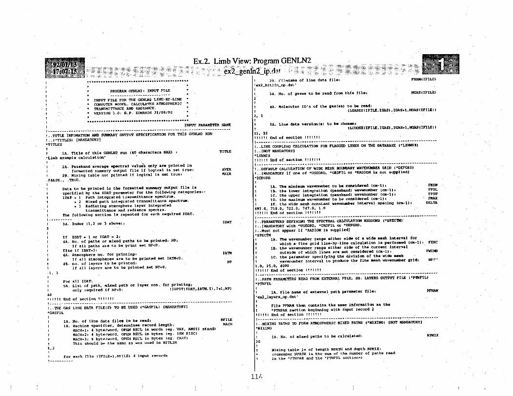
Ex.2. Limb View: Program GENLN2e : :ex2 gen . i .. :; .. : . .. :..

.***************+t-*******+*+t***+* *

,!~ ~ * PROGRAM GENLN2: INPUT FILE

1 , e * ____________-------------------

! * INPUT FILE FOR THE GENLN2 LINE-BY-LINE~! ,~ * COMPUTER MODEL. CALCULATES ATMOSPHERIC

!? * TRANSMITTANCE AND RADIANCE.!, * VERSION 3.0: D-P. EDWARDS 21/08/90

! INP%!…----- -------------------------- ____ ______ _ --

!..TITLE INFOMATION AND SUMMARY OUTPUT SPECIFICATION FOR THIS Gl

!..(*TITLES) [MANDATORY)*TITLES

! 1A. Title of this GENLN2 run (40 characters MAX) :

'Limb example calculation'

2A. Passband average spectral values only are printed in

! formatted summary output file if logical is set true

! 2B. Mixing table not printed if logical is set true:

.FALSE., .TRUE.

Data to be printed in the formatted summary output file

specified by the IDAT parameter for the following catego

IDAT -1 Path integrated transmittance spectrum.

! 2 Mixed path integrated transmittance spectrum.

.3 Radiating atmosphere layer integrated

I| ~ ~transmittance and radiance spectra.The following section is repeated for each required IDAT

-_---------

! 3A. Index (1,2 or 3 above):3

If IDAT * 1 or IDAT = 2:! 4A. No. of paths or mixed paths to be printed: NP;

! if all paths are to be print set NP<0.

Else if IDAT=3:! 4A. Atmosphere no. for printing:

if all atmospheres are to be printed set IATM<0.

4B. no. of layers to be printed:* if all layers are to be printed set NP<0.

-1, 1

* For all IDAT:! 5A. List of path, mixed path or layer nos. for printing;

! only required if NP>0: (IOPDT(IDA

40!!!,! End of section !1!I!lI!---------------------------------_-_-_-_ _ _ _

!..THE GAS LINE DATA FILE(S) TO BE USED (*GASFIL) (MANDATORY]

*GASFIL

! 1A. No. of line data files to be read:

I lB. Machine specifier, determines record length:MACHIl: 4 byte/word, OPEN RECL in words (eg. VAX, AN

MACH=2: 4 byte/word, OPEN RECL in bytes (eg. IBM RIS

MACH=3: 8 byte/word, OPEN RECL in bytes (eg. CRAY)

This should be the same as was used in HITLIN

1,2

For each file (IFILE=1,NFILE) 4 input records,----------

! 2A. Filename of line data file: FNAM(IFILE)

'ex2_hit 1n_op.dat'

3A. No. of gases to be read from this file: NGAS(IFILE)

2

: 4A. Molecular ID's of the gas(es) to be read:LGASES(IFILE,IGAS), IGGA1,NGAS(IFILE))

2, 3

lT PARAMETER NAME I SA. Line data version(s) to be chosen,

____------- ____I! (LCHOSE(IFILE,IGAS),IGAS1.,NCGAS(IFILE))

ENLN2 RUN 11, 10!!1!11 End of section 1! !!M1!---------------------------------------_------_--_____________________________!..LINE COUPLING CALCULATION FOR FLAGGED LINES ON THE DATABASE (*LINMIX)

TITLE I.. NOT MANDATORY]*LINMIX!! !!! End of section ! ! !!

AVER !..DEFAULT CALCULATION OF WIDE MESH BOUNDARY WAVENUMBER GRID (*DEFGRD)

MXER !.. MANDATORY if one of *USEGRD, *GRDFIL or *RADIOM is not supplied)

*DEFGRD

is , 1A. The minimum wavenumber to be considered (cm-l): FMIN

ries:- 1B. the lower integration (passband) wavenumber (cm-l): FPSL

I 1C. the upper integration (passband) wavenumber (cm-l): FPSU

! D. the maximum wavenumber to be considered (cm-1): FMAX

, 1E. the wide mesh constant wavenumber interval spacing (cm-l1) DELTA

693.0, 718.0, 722.0, 747.0, 1.0?>. !,, ~!! !II End of section !! ! I

!--------------------------------------- --_--------___________________________

IDAT I..PARAMETERS DEFINING THE SPECTRAL CALCULATION REGIONS (*SPECTM)

I..(MANDATORY with *USEGRD, *GRDFIL or *DEFGRD.

I..Must not appear if *RADIOM is supplied]*SPECTM

1A. The wavenumber range either side of a wide mesh interval for

I which a fine grid line-by-line calculation is performed (cm-1): FEXC

! B. the wavenumber range either side of the current interval

lATMH outside of which lines are not considered (cm-l): FWIND

! 1C. the parameter specifying the division of the wide mesh

NP ! wavenumber interval to produce the fine mesh wavenumber grid: NDIt'

1.0, 25.0, 4000i!!!I! End of section !!!I!!!

------------------------------------ ----- -----------------------------------

!..PATH PARAMETERS READ FROM EXTERNAL FILE, EG. LAYERS OUTPUT FILE (*PTHFIL)

*PTHFILT. IATM,I), Il,NP) !

! 1A. File name of external path parameter file: PFNAN

'ex2_layers_op.dat'

! File PFNAM then contains the same information as the

! *PTHPAR section beginning with input record 2

!!!I!! End of section H!!!i!!

NFILE! . ---.----------------------------.--------.---------------------- --- --- -

MACH I..MIXING PATHS TO FORM ATMOSPHERIC MIXED PATHS (*MIXING) (NOT MANDATORY]

ISII stand) *MIXINGSC) !

! 1A. No. of mixed paths to be calculated: NPMIX

20

! Mixing table is of length NPATH and depth NPMIX:(remember NPATH is the sum of the number of paths read

in the *PTHPAR and the *PTHFIL sections)

114

Ex.2. Limb View: Program GENLN2**---*...-.--. ..-. ,..* . - .-....-.P. .d.... . . ...........-..

! The required mixing table parameters are:-2A. The mixed path index: IPMIX

! 2B. the mixing table: (TABMIX(IPATH,IPMIX),IPATHl1,NPATH))! Each new mixed path must begin a new line, and the! input field must not exceed 130 characters.!

1 ROTO 1 ROT19 ROTO 1 ROT192 ROT1 1 ROT18 ROT1 1 ROT183 ROT2 1 ROT17 ROT2 1 ROT174 ROT3 1 ROT16 ROT3 1 ROT165 ROT4 1 ROT15 ROT4 1 ROT156 ROTS 1 ROT14 ROTS 1 ROT147 ROT6 1 ROT13 ROT6 1 ROT138 ROT7 1 ROT12 ROT7 1 ROT129 ROT8 1 ROT11 ROT8 1 ROT11

10 ROT9 1 ROT10 ROT9 1 ROT1011 ROT10 1 ROT9 ROT10 1 ROT912 ROT11 1 ROT8 ROT11 1 ROT813 ROT12 1 ROT7 ROT12 1 ROT714 ROT13 1 ROT6 ROT13 1 ROT615 ROT14 1 ROTS ROT14 1 ROTS16 ROT15 1 ROT4 ROT15 1 ROT417 ROT16 1 ROT3 ROT16 1 ROT318 ROT17 1 ROT2 ROT17 1 ROT219 ROT18 1 ROT1 ROT18 1 ROT120 ROT19 1 ROTO ROT19 1 ROTO

I!!I ! End of section I! !!!I---------------------------------------

!..RADIANCE CALCULATION (*RADNCE) [NOT MANDATORY)*RADNCE!

! 1A. No. of radiating atmospheres to be calculated: NATH

3! For each atmosphere (IATM=1,NATM) 3 input records

! Layer table data consists of the following:-2A. The radiating atmosphere index: IATM

! 2B. the viewing parameter: IVIEW(IATM)

! 2C. the layer emission parameter: IEMS(IATM)

! 2D. the no. of layers in the atmosphere: NLAY(IATM)

! 2E. path or mixed path specifer for total layer absorption: LAYSP(IATM)2F. the path (LAYSP(IATM)=1) or mixed path nos.(LAYSP(IATM)=2)

! to be used to specify the layer total absorption in order

! of radiation travel: (LAYER(ILAY,IATM),ILAY=1,NLAY(IATM))1, 1, 2, 40, 220 19 18 17 16 15 14 13 12 11 10 9 8 7 6 5 4 3 2 11 2 3 4 5 6 7 8 9 10 11 12 13 14 15 16 17 18 19 20

! If IVIEW(IATM)-2 then the initiating surface parameters are supplied:! 3A. Atmospheric boundary temperature (K): TBDY(IATM)! 3B. temperature of the initiating surface: TINIT(IATM)

I 3C. emissivity of initiating surface: EMSTY(IATM)

ITBDY(1), TINIT(l), EMSTY(1)

If IEMS(IATM)=2 different paths/mixed paths can to be used for

I ,layer emission to those used for layer transmittance:! 4A. path or mixed path specifer for emission layer absorption:LEMSP(IATH)! 4B. the path (LEMSP(IATM)=1) or mixed-path nos.(LEMSP(IATM)=2)! to be used to specify the layer emission in order! in order of radiation travel: (LAYEMS(ILAY,IATM),ILAY=1,NLAY(IATM))120 19 18 17 16 15 14 13 12 11 10 9 8 7 6 5 4 3 2 11 2 3 4 5 6 7 8 9 10 11 12 13 14 15 16 17 18 19 20!---- -----

2, 1, 2, 40, 22, 1, 2, 40, 220 19 18 17 16 15 14 13 12 11 10 9 8 7 6 5 4 3 2 11 2 3 4 5 6 7 8 9 10 11 12 13 14 15 16 17 18 19 20140 39 38 37 36 35 34 33 32 31 30 29 28 27 26 25 24 23 22 2121 22 23 24 25 26 27 28 29 30 31 32 33 34 35 36 37 38 39 40

3, 1, 1, 40, 220 19 18 17 16 15 14 13 12 11 10 9 8 7 6 5 4 3 2 11 2 3 4 5 6 7 8 9 10 11 12 13 14 15 16 17 18 19 20! ! !! End of section !!!!!!

I..INTEGRATION SWITCH (*INTEGN) [NOT MANDATORY)*INTEGNI Logical switch. When present the transmittance and radianceI spectra are integrated over each wide mesh interval.I!!!! ! End of section !!!!!!

I..UNFORMATTED OUTPUT FILE SPECIFICATION (*OUTPUT) (NOT MANDATORY)OUTPUT

1A. File name of output file: OPFNAM

'ex2_genln2_ops. dat'

Data to be output is specified by IDAT parameterfor the following categories:-IDAT= 1 Path point transmission spectrum;

= 2 Path integrated transmission spectrum;! 3 Mixed path point transmission spectrum;! I 4 Mixed path integrated transmission spectrum;! = 5 SLayer point transmission spectrum;

! 6 Layer integrated transmission spectrum! 7 Layer point radiance spectrum;* 8 Layer integrated radiance spectrum.

I The following section is repeated for each required IDAT.!----------

2A. Index (1 thro' 8 above): IDAT5

For IDAT 1, 2, 3 or 4:3A. no. of paths or mixed paths to be output: NP

i f all paths are to be output set NP<O.! For IDAT = 5, 6, 7 or 8:I 3A. atmosphere no. for output: IATM

if all atmospheres are to be output set IATM<0.3B. no. of layers to be output: NP

if all layers are to be output set NP<O.-1,1

I For all IDAT:4A. List of path, mixed path or layer nos. for output;

I only required if NP>O: (IOPGR(IDAT,IATM,I),I=1,NP)40

7-1,140I----------!!ilI End of section !!!!!!

!..END OF GENLN2 INPUT (*ENDINP) [MANDATORY]*ENDINP!!!!! ! End of input data to GENLN2 !!!!!!

115

' ' .,. ' .: .., ;, . . . -- 7- I " I , ... .. . .. .. . .

Limb View: Piex2 . ..en ...

********* **************************************

** GENLN2: GENERAL LINE-BY-LINE ATMOSPHERIC **

** TRANSMITTANCE AND RADIANCE MODEL **

** VERSION 3.0 D.P. EDWARDS 27/02/91 **

** (C) COPYRIGHT 1991 UCAR/NCAR **

** ALL RIGHTS RESERVED **

** GENLN2 SOFTWARE AND RELATED MATERIALS **** MAY BE USED ONLY UNDER AN EXECUTED VALID **

** LICENCE AGREEMENT **************************** ** **********4

***********t******** ********************

DATE (DAY.MON.YR): 10.12.91

*************** CHECK INPUT DATA FOR ERRORS ***************

&&&&&&&&&&&&&&&&&&&&&&&&&&& & && & &&& & &&&&& &&&&&&&&&&&&&&&&&&&&&&&&&&&&&&&&&&&&&&&&&&&&&&&&&&&&&&&&&&&&&&&&&&&&&&&&&&&&&&&&&&&&&&&&&&&

************** INPUT DATA SUCCESSFULLY READ ***************

*************** SUMMARY OF INPUT DATA ***************

TITLE OF THIS RUN :- Limb example calculation

I I I I IIIIIIII I II I I I I I I I I I I I I I I I I I I I1 III11I1111 I I I I I I I I 11 I 11 I 1111I l I 1111111111111 IIII11111 111

LINE AND CROSS-SECTION DATA***************************

1 LINE DATA FILE(S) WILL BE USED

FILE NO. 1 FILENAME ex2_hitlin_op.dat

2 GAS(ES) TO BE READ, MOLEC ID NO(S):- 2 3

GAS LINE VERSION(S) TO BE CHOSEN:- 11 10

LINE MIXING SWITCHED ON

| 1 1 1 1 | | 1! 111! 1 11111t 11111 I111I1 11 1I 11111 I I11! 1 1111 II11!I 11!1 11111 1 1 11 1 t11 1 ll11 11 11I 1 1111

WAVENUMBER GRID***************

TOTAL WAVENUMBER RANGE CONSIDERED 693.000 - 747.000 cm-l

PASSBAND (INTEGRATION) WAVENUMBER RANGE 718.000 - 722.000 cm-1

THIS CONSISTS OF 4 INTERVALS OF AVERAGE WAVENUMBER WIDTH 1.000 cm-1

EACH INTERVAL WILL BE DIVIDED INTO 4000 FINE MESHES FOR THE TRANSMITTANCE CALCULATION.

I I I II 1 1 ! !! I I II I 1111 1 II I I I II 1I '11 111 1 11111 I I1 I I II 1 I 1 I ! I I 1 I 1 I III IIII II I 11111 11 1 111 1 11111 I II 1 I 1111 1 1111 I

TRANSMITTANCE CALCULATION*************************

THE LINE ABSORPTION IN A RANGE OF 1.000 cm-1 EITHER SIDE OF THE WIDEMESH INTERVAL WILL BE TREATED EXPLICITLY.

THE WING ABSORPTION DUE TO LINES LYING IN THE RANGE 1.000 - 25.000 cm-1

EITHER SIDE OF THE WIDEMESH INTERVAL WILL BE INCLUDED.

THE CONTINUUM ABSORPTION WILL BE INCLUDED FOR APPROPRIATE PATHS.

!I 111P D!!!!!I!! !!! ! 111

PATH DATA*********

116

Ex.2. Limb View: Program GENI|.. .......... ..'· ···; ::::i ··::::::::::::::· ::::: ·····::::: ····· :::: · i i i i' ' ' ' ···:: :: · :::i:: ···· ·:: k:: : ·: ::

I:.::i::::::··:.:·::::::::: i:::::ii ·: ·:·:·..·:: ···· i:::,ij ii~ :: ··: i i... .... ... :::::9i:· ::··: : ··· : ·-·::·: 1,

PATH FILE GAS ID ISO ID AMT kg.moles/cm2 T K P atm PARTP atm VEL m/s LINESHAPE CONTINUUM

1 1 2 0 1.637E-06 226.728 1.151E-02 3.799E-06 O.OOOE+00 VOIGTC02 CON

2 1 2 0 6.165E-07 227.525 1.051E-02 3.467E-06 0.000E+00 VOIGTC02 CON

3 1 2 0 7.719E-07 228.541 9.357E-03 3.088E-06 0.000E+00 VOIGTC02 CON

etc.

37 1 3 0 1.192E-10 255.225 3.262E-04 5.231E-10 0.000E+00 VOIGT NOCON

38 1 3 0 3.643E-11 241.444 1.659E-04 1.635E-10 O.000E+00 VOIGT NOCON

39 1 3 0 9.990E-12 228.137 8.307E-05 5.121E-11 0.000E+00 VOIGT NOCON

40 1 3 0 3.562E-12 211.583 3.158E-05 8.882E-12 0.000E+00 VOIGT NOCON

IIIItIIIII III II I I II II i IIIII I I I ll II1 1 I I

MIXING TABLE DATA**************

MIXING TABLE IS OF LENGTH 40 PATH(S) AND DEPTH 20 MIXED PATH(S)

RADIANCE DATA

CALCULATIONS WILL BE PERFORMED FOR 3 RADIATING ATMOSPHERE(S)

ATMOSPHERE NO LAY PTH/MIX PATH/MIXED PATH NOS TO BE USED FOR LAYER TRANSMITTANCE IN ORDER OF THE DIRECTION OF RADIATION TRAVEL

1 40 2 20 19 18 17 16 15 14 13 12 11 10 9 8 7 6 5 4 3 2 1 1 2 3 4

6 7 8 9 10 11 12 13 14 15 16 17 18 19 20

VIEWING PARAMETER = 1

EMISSION PARAMETER = 2 PATH/MIXED PATH NOS TO BE USED FOR LAYER EMISSION IN ORDER OF THE DIRECTION OF RADIATION TRAVEL

1 20 19 18 17 16 15 14 13 12 11 10 9 8 7 6 5 4 3 2 1 1 2 3 4 5

6 7 8 9 10 11 12 13 14 15 16 17 18 19 20

2 40 2 20 19 18 17 16 15 14 13 12 11 10 9 8 7 6 5 4 3 2 1 1 2 3 4 5

6 7 8 9 10 11 12 13 14 15 16 17 18 19 20

VIEWING PARAMETER = 1EMISSION PARAMETER = 2 PATH/MIXED PATH NOS TO BE USED FOR LAYER EMISSION IN ORDER OF THE DIRECTION OF RADIATION TRAVEL

1 40 39 38 37 36 35 34 33 32 31 30 29 28 27 26 25 24 23 22 21 21 22 23 24 25

26 27 28 29 30 31 32 33 34 35 36 37 38 39 40

3 40 2 20 19 18 17 16 15 14 13 12 11 10 9 8 7 6 5 4 3 2 1 1 2 3 4 5

6 7 8 9 10 11 12 13 14 15 16 17 18 19 20

VIEWING PARAMETER = 1

SPECTRA WILL BE INTEGRATED OVER THE WIDEMESH INTERVALS.

*************** CALCULATION BEGINS **************

*************** ELAPSED CPU TIME: 0:54:44.87 ***************

117

yx.2. Limb View: Program GEN^ij. ie.:.'.·.. . .:`I ^ ^.. . . . . . . . . . ..... .

*************** CALCULATION COMPLETE. ***************

INTEGRATED ATMOSPHERIC LAYER TRANSMITTANCES AND BOUNDARY RADIANCES***********************************

*** ATMOSPHERE 1 ***

*** LAYER NO. 40 ***INTERVAL LOW BDY cm-1 UPP BDY cm-1 FINE MESHES TRANSMITTANCE BDY RADIANCE

W/(m2.sr.cm-1)

1 718.000 719.000 4000 .496800E+00 .209419E-01

2 719.000 720.000 4000 .286851E+00 .356913E-01

3 720.000 721.000 4000 .618608E-01 .546551E-01

4 721.000 7-2.000 4000 .611289E+00 .131767E-01

AVERAGE VALUES OVER PASSBAND , .364200E+00 .311162E-01

*** ATMOSPHERE 2 ***

*** LAYER NO. 40 ***

INTERVAL LOW BDY cm-1 UPP BDY cm-1 FINE MESHES TRANSMITTANCE BDY RADIANCEW/(m2.sr.cm-1)

1 718.000 719.000 4000 .496800E+00 .749775E-02

2 719.000 720.000 4000 .286851E+00 .500115E-02

3 720.000 721.000 4000 .618608E-01 .483975E-02

4 721.000 722.000 4000 .611289E+00 .840466E-02

AVERAGE VALUES OVER PASSBAND .364200E+00 .643582E-02

*** ATMOSPHERE 3 ***

*** LAYER NO. 40 ***

INTERVAL LOW BDY cm-1 UPP BDY cm-1 FINE MESHES TRANSMITTANCE BDY RADIANCEW/(m2.sr.cm-1)

1 718.000 719.000 4000 .496800E+00 .284394E-01

2 719.000 720.000 4000 .286851E+00 .406923E-01

3 720.000 721.000 4000 .618608E-01 .594947E-01

4 721.000 722.000 4000 .611289E+00 .215815E- 01

AVERAGE VALUES OVER PASSBAND .364200E+00 .375520E-01

*************** END OF DATA OUTPUT ***************

*************** GRAPHICS FILE WRITTEN TO: ex2_genln2_ops.dat *********

118

Ex.2. Limb View: Program GENGRIexz.Igengi

IIIIfIII1I I II#I'Im IIIIIIi0im fIIIIIII11111

II PROGRAM GENGRP II# ------------ II

II GENERAL PURPOSE GRAPHICS FOR PLOTTING III GENLN2 TRANSMITTANCE AND RADIANCE SPECTRA IIII VERSION 3.0 D.P. EDWARDS 27/02/91 IIII (C) COPYRIGHT 1991 UCAR/NCAR IIII ALL RIGHTS RESERVED 11II GENLN2 SOFTWARE AND RELATED MATERIALS MAY IIII BE USED ONLY UNDER AN EXECUTED VALID IIII LICENCE AGREEMENT III1 IIIIIIIIIIIIII1111 11111111111 111 "111111

IIIII"IIIIIIIIIIIII1IIIIIIII IIIIIIIII11IIIIIIIII

**Q** Name of GENLN2 unformatted output file to plot?:ex2_genln2_ops dat**Q** Enter filename of output graphics metacode file :ex2_gengrp_trans meta**Q** Do you want the default picture size Y/N :Y**Q** For a default axis, the axis drawn will be

that appropriate for the first curve entered.Is a default X-axis to be drawn? (Y/N :

Y**Q** Is a default Y-axis to be drawn? (Y/N] :Y**Q** Enter the no. of curves to be plotted on this graph?1**Q** Do you want to supply your own curve captions? [Y/N :YI1111 CURVE NO. 1 II#1**Q** Is a path transmittance spectrum (PT),

a mixed path transmittance spectrum (XT),a radiating atmosphere layer transmittance spectrum (AT),or a radiating atmosphere layer radiance spectrum (AR)to be plotted?Enter one of PT, XT, AT or AR:

AT**Q** Curve 1. IATM no. of layer atmosphere? :3**Q** Curve 1. ILAY no. of layer to be plotted? :40**Q** Are wide mesh binned spectral values to be plotted? [Y/N]:N»*Q** Enter line type and pen type for drawing curve LTYPE,IPEN :1,2**Q** Enter curve caption, 50 chars. max. :Total transmittance, 30km tangent height**Q** Do you want to degrade the spectra with an

instrument line shape (ILS) function? [Y/NI :Y**Q** ILS function type specifier;

1 = square boxcar2 = triangle3 = Fourier spec. (only with evenly spaced points)4 = user supplied (only with evenly spaced points)Enter 1,2,3 or 4

3*Q** Enter max. retardation length in cm:50 0

_ trans.aa ,i :**Q** Fourier apodization specilfer;

1 = no apodization2 = triangular apodization3 = Norton & Beer weak apodization4 = Norton & Beer medium apodization5 = Norton & Beer strong apodizationEnter 1,2,3,4 or 5

4**Q** Are all points to be plotted? (Y/N IN**Q** Enter no of plot points/cm-1200**Q** Is an external spectra to be plotted? (Y/N):N

119

.E.. ......... -.

I

GENLN2, TRANSMITTANCE SPECTRUM

1 .0

.9

.8

.7

.6

.5

.4

.3

.2

.1

718.5 719.0 719.5 720.0 720.5 721.0 721.5 722.0WAVENUMBER cm-1

Limb example calculation

0

I Total transmittance, 30km tangent heightI

120

1.0

.9

.8

.7

.6

.5

.4

wz

<

I-

.3

.2

.1

0718.0

Ex.2. Limb View: Program G]

8"I:. Bj··-~.·;,II-~"'lB ';r':I·::·~il·;.:i'.;:i':-:(ii'-:- l:ilR^-

IIIIIIiiIIIIIIi«iII PII11 GENERAL PURPOSII GENLN2 TRANSHIII VERSION 3.0II (C) COPYRIGHTII ALL RIGHTS RESI GENLN2 SOFTWARII BE USED ONLY UII LICENCE AGREEM

IIIIIIIIIIIIIIIII11100011110011111

**Q** Name of GENLex2_genln2_ops.dat**Q** Enter filenaex2_gengrp_rad.met**Q** Do you wantY"*Qe* For a defaul

that approprIs a default

Y**Q'* Is a defaultY**Q** Enter the no2

gIIIIIIIIIIIIIII01I11100000IIIIIIIIIII0110000010000IIIIIIIII

ROGRAM GENGRP 10_-----__---- _I

E GRAPHICS FOR PLOTTING IITTANCE AND RADIANCE SPECTRA IID.P. EDWARDS 27/02/91 11991 UCAR/NCAR IIERVED IIE AND RELATED MATERIALS MAY ItNDER AN EXECUTED VALID I 3IENT I11 «111*1§11 1111111«11111IIIIIII t111t111111g11111111

112 unformatted output file to plot?:

kme of output graphics metacode file:athe default picture size [Y/N :

t axis, the axis drawn will beiate for the first curve entered.X-axis to be drawn? (Y/N) :

Y-axis to be drawn? (Y/N1

. of curves to be plotted on this graph?

**Q** Do you want to supply your own curve captions? [Y/N :

Y0I0i0 CURVE NO. 1 Illl***Q** Is a path transmittance spectrum (PT),

a mixed path transmittance spectrum (XT),

a radiating atmosphere layer transmittance spectrum (AT),

or a radiating atmosphere layer radiance spectrum (AR)to be plotted?Enter one of PT, XT, AT or AR:

AR**Q** Curve 1. IATM no. of layer atmosphere? :

1**Q** Curve 1. ILAY no. of layer to be plotted? :40**Q** Are wide mesh binned spectral values to be plotted? [Y/N :

N*Q** Enter line type and pen type for drawing curve LTYPE,IPEN:

1,2**Q** Enter curve caption, 50 chars. max.:C02 radiance, 30km tangent height111i1 CURVE NO. 2 10111**Q** Is a path transmittance spectrum (PT),

a mixed path transmittance spectrum (XT),a radiating atmosphere layer transmittance spectrum (AT),or a radiating atmosphere layer radiance spectrum (AR)

to be plotted?Enter one of PT, XT, AT or AR:

AR*Q** Curve 2. IATM no. of layer atmosphere?:

2**Q** Curve 2. ILAY no. of layer to be plotted? :40

**Q** Are wide mesh binned spectral values to be plotted? (Y/N] )N**Q** Enter line type and pen type for drawing curve LTYPE,IPEN ,2,3"*Q** Enter curve caption, 50 chars. max. z)3 radiance, 30km tangent height**Q** Do you want to degrade the spectra with an

instrument line shape (ILS) function? (Y/N :Y·*Q** ILS function type specifier;

1 = square boxcar2 = triangle3 - Fourier spec. (only with evenly spaced points)4 = user supplied (only with evenly spaced points)Enter 1,2,3 or 4

3·*Q** Enter max. retardation length in cm:50.0'*Q** Fourier apodization specifier;

1 = no apodization2 = triangular apodization3 = Norton & Beer weak apodization4 = Norton & Beer medium apodization5 = Norton & Beer strong apodizationEnter 1,2,3,4 or 5 :

4**Q** Are all points to be plotted? [Y/N :

**Q** Enter no of plot points/cm- :200**Q** Is an external spectra to be plotted? [Y/N] =N

121

- , , : .., , -`:.: :: m :::: 7:.: .: . . , -, , - . , , . : : ..: . ... .. -: ,'· ..:7 : .. , - .

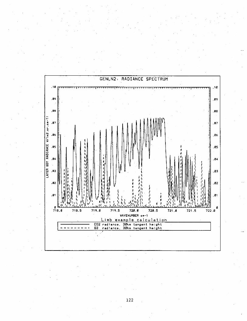
GENLN2. RADIANCE SPECTRUM

.10

.09

.08

-

* .07u

L

Cu6 .06

Nu .05z

cx

' .04

0

U .03

-J

.02

.01

718.0 718.5 719.0 719.5 720.0 720.5

WAVENUMBER cm-1Limb examDle calculation

721.0 721.5 722.0

C02 radiance. 30km tangent height- - - 03 radiance, 30km tangent height

JI'

122

.10

.09

.08

.07

.06

.04

.03

.02

.01

00

APPENDIX 3. EXAMPLE PMR CALCULATION

A3.1 Overview of Example PMR Calculation

This appendix describes how GENLN2 can be used to model a pressure modulatorradiometer (PMR). A PMR is a gas correlation radiometer in which the atmospheric radiationpasses through a cell containing the same gas as the atmospheric gas which is being measured.The gas pressure inside the cell is modulated, resulting in a modulation in the opacity of thecell due to that component of the atmospheric radiation that was emitted by the cell gasspecies. This produces fluctuations in the signal at the detector only inside the spectral linesof the gas species contained in the cell. High effective resolution and signal-to-noise ratioare possible because contributions from all lines of the cell gas species are sampled. Theprinciples and operation of PMRs are discussed in detail by Taylor (1983). The pressurecycle used in the cell determines the part of the spectral line that is sampled. A widebandradiometer mode is also possible and is achieved by asynchronously chopping the input signalwith the pressure modulation to measure the mean radiation transmitted by the cell.

The following discussion briefly sets out the method. This is followed by a simple workedexample that demonstrates the running of the various programs.

A3.2 Modelling the PMR Response Functions

Let I(v, Zobs) be the radiation in W/(m 2 .sr.cm- l ) falling on a radiometer. For a radio-metrically self-calibrating instrument the signal R is the ratio between the atmospheric andblackbody emission

R -So I(v, Zob,)F(v)dvfo B(v TB)F()dv

where F(v) is the total radiometer response function and B(v, TB) is the blackbody radianceat the reference temperature TB.

The total radiometer response can be written as the product of the response profile ofthe wide band channel blocker, G(v), and the gas correlation response, H(v),

F(v) = G(v) H(v). (A3.2)

Assume now that the radiometer channel blocker response profile G(v) varies very slowlyover the wavenumber width of a GENLN2 wide mesh interval width 6v. If there are N widemesh intervals i, which need not have equal spacing, then Eqn.A3.1 can be written

"N C~iS~i I (V, Z,,bs) H (v) dV11-pN~~~~~ -~~(A3.3)

-i= Gi fS B(v, TB)H(v)dv

whereG= 16vi GQ)dv. (A3.4)

The ISAMS instrument aboard the Upper Atmosphere Research Satellite (UARS) mission(Reber, 1985) uses several PMRs for sounding various atmospheric gases. The two functionsG(v) and H(v) for the CO 2 channel 7.1 PMR, defined in Section A3.4, are shown in Fig.A3.1.

123

A3.3 The Gas Correlation Response Function

A schematic diagram of a PMR is shown in Fig.A3.2. At the center of a purely collisionbroadened spectral line the PMR absorption for a given cell length and temperature is inde-pendent of cell pressure and the radiometer response is zero. Away from the line center theresponse rises to a maximum and then decreases, the exact form depending on the opticalthickness. For the optically thin case, the maximum occurs at line center±/v where aL isLorentz half width evaluated at the cell mean pressure, see Fig.A3.3. The insert on Fig.A3.1shows an enlargement of the PMR response function for the ISAMS CO 2 channel 7.1 exam-ple PMR and shows the double maximum and central depression. If Doppler broadening isalso present then the absorption at line center is greater during the high-pressure part of themodulator cycle and the response is greater than zero. If the temperature or cell length alsovary then the response can be positive or negative.

The PMR cycle can be represented as a linear combination of M gas cells each containingthe PMR gas. Each cell has the same length but the pressure and possibly the temperaturediffer according to the point that the cell represents on the modulation curve. The gas corre-lation response is then approximated as a weighted linear combination of the monochromatictransmittances of each cell

M

H(v) = Eaj j() (A3.5)j=l

where Trj(v)cel is the transmittance of cell j and aj is the weighting coefficient. In thisway the commonly used two-cell approximation is modelled by setting M = 2, cell 1 is thehigh pressure cell with al = -1 and cell 2 is the low pressure cell with a 2 = +1. The gascorrelation response in this case is

H(v) = 2(v)l°tO p cell _ rl ()high p cell (A3.6)

The two-cell wideband calculation is modelled by setting both a, and a2 to 0.5 withthe same cell transmittances. For a sinusoidal pressure cycle, cells can be defined at varioustimes along the cycle with the corresponding pressure, temperature, and gas amount. Theweight of each cell is then equal to the sine of the time at which the cell is defined. For asymmetric modulator cycle, the sum of the coefficients in the PMR case should be zero andin the wideband case it should be unity.

The gas correlation response function H(v) depends on the PMR cell pressure andtemperature cycles. Thus the same function will be applicable to many atmospheric radiancecalculations that use the same PMR. The approach taken in GENLN2 is to pre-computeH(v) for a particular PMR on the fine wavenumber grid and to store the result in a filefor subsequent GENLN2 atmospheric calculations to use. This avoids duplication of celltransmittance calculations and makes possible a PMR representation with a larger numberof composite cells.

Away from strong absorption lines of the PMR cell gas, the response function H(y)approaches zero. At such points it is unnecessary to compute the line-by-line radiance. TheGENLN2 wide mesh wavenumber boundaries are chosen such that they fall either side ofregions of non-zero response. Wide meshes with zero response are then flagged. Becausethe response function and the wide mesh boundaries are input at the start of the GENLN2calculation, line-by-line calculation in these meshes can be switched off to save time.

124

A3.4 Example PMR Calculation: ISAMS CO 2 Channel 7.1

There follows a description of the stages for modelling a PMR using GENLN2. Theexample is that of the ISAMS instrument CO2 channel 7.1. A simple 2-cell PMR calculationis used for a 30 km tangent height limb view of the atmosphere.

The spectral region of interest is 590-640 cmn with the channel center at 615 cm- .Assume a CO2 PMR with a 40 mb mean pressure and compression ratio of 2.5.The cell length is 30 mm.The reference blackbody temperature TB is 296 K.The Cell temperature, which is assumed constant, is 290 K.

Using the 2-cell approximation:Cell 1: Low pressure = 2.5 - 0.5 x 40 mb = 25.2982 mb = 0.02496 atmGas amount = 3.06315 x 10- 9 kg.moles.cm- 2

Cell 2: High pressure = 2.5+0 5 x 40 mb = 63.2455 mb = 0.06242 atmGas amount = 7.65788 x 10- 9 kg.moles.cm-2

A3.5 Program GENLN2: Calculation of the cell transmittances

In the discussion that follows it is assumed that the reader is familiar with the usualstages of a GENLN2 calculation as described in example calculations 1 and 2. The emphasishere will be on those stages specific to the PMR calculation. The previously calculated linedata file ex2hJitlinop.dat is used, Section A2.2.

The first task is to calculate the gas correlation response function H(v). This is achievedwith a run of GENLN2 where the gas paths that are defined in the *PTHPAR section of theinput file represent the cells of the modulation cycle, see ex3_genln2ipr.dat. It is importantthat the gas amount for each cell is consistent with the cell pressure and it is wise to givethese quantities to several significant figures. The wavenumber range and resolution of thiscalculation must correspond to those required for the eventual atmospheric calculations. Thepath transmittances calculated on the fine wavenumber grid, IDAT=1 in *OUTPUT are writtento the unformatted output file ex3_genln2_opsr. A listing is given of the formatted outputsummary file ex3_genln2_opdr.dat.

A3.6 Program PMRFIL

The interactive program PMRFIL is used at this stage. This consists of two subroutines:

PMRFIL- Main program. Manages input and output, calculates the gas correlationresponse function filter on the fine wavenumber grid. Unit 6 is used to writeinteractive questions and unit 5 to read the answers. Unit 10 is used to readthe GENLN2 unformatted output file.

PMREXT- Subroutine. Calculates the wide mesh wavenumber interval boundaries tocorrespond with region of non-zero filter response. Intervals of zero responseare flagged. Unit 30 is used to write the output filter response data file.

Input to this program consists of the GENLN2 output file ex3_genln2_opsr.dat andthe user will be prompted for the path number to be associated with each cell and the cellweighting coefficients described in Section A3.3. The input dialogue for this calculation isshown in ex3_pmrfilip.dat.

The program first performs the linear combination of weighted cell transmittances. Theoptimal wide mesh wavenumber boundaries are then calculated. The user is prompted for

125

the minimum absolute value of H(v) to be treated as non-zero, the maximum number offine grid points per wide mesh interval, the maximum number of wide meshes, and thewide mesh spacing. The values chosen for these quantities should be consistent with themaximum array sizes chosen for the subsequent GENLN2 calculations. The code identifiesregions of predominantly non-zero response and these are enclosed by wide mesh wavenumberboundaries. The boundaries are then adjusted iteratively to satisfy the input criteria. Zeroresponse wide meshes are flagged so that the subsequent GENLN2 line-by-line calculation isswitched off.

This and the previous calculation stages need only be performed once for a particularPMR. The output response file ex3_pmrfilop.dat is stored and used for all subsequentGENLN2 atmospheric radiance calculations that use this PMR.

A3.7 Program GENLN2: Atmospheric Calculation

The calculation is performed for 30 km tangent height limb view of the U.S. 1976 Stan-dard atmosphere. Two gases, CO2 and 03, are included in each layer. The atmosphere isassumed to be the same as that of example calculation 2 and the same set of path datafrom ex2Jayersop.dat are used by GENLN2, See Section A2.3. Line data is taken fromthe previously calculated line data file ex2_hitlinop.dat, Section A2.2. Line coupling isincluded in the calculation as described in Section A2.4.

The wavenumber grid for a PMR calculation is defined using *RADIOM input option.This keyword input section is described below. See also Table 4.1 and the input wavenumberparameters illustrated in Fig.4.1.

*RADIOMThis section is used to input the wavenumber parameters for a GENLN2 calculation usinga radiometer spectral filter. It must not be used in conjunction with the equivalent inputsections *USEGRD, *GRDFIL, *DEFGRD, or *SPECTM. (1A) FEXC (real) is the wavenumber rangein cm - ' either side of a wide mesh interval for which the fine-pass calculation is performed.For wide mesh interval IPW a line-by-line absorption calculation is performed over the finewavenumber grid FF(IPT,IPW) for line center wavenumbers WNUM cm-1 falling in the rangeFBDY(IPW+NPL-1) - FEXC < WNUM < FBDY(IPW+NPL) + FEXC

(1B) FWIND (real) is the wavenumber range cm -1 either side of a wide mesh interval outsideof which lines are not considered. The line wing absorption calculation is performed over thethree wavenumber points FW(IP,IPW) of the wide mesh for line center wavenumbers WNUMcm- 1 falling in the rangesFW(IP,IPW) - FWIND < WNUM < FBDY(IPW+NPL-1) - FEXC andFW(IP,IPW) +FWIND > WNUM > FBDY(IPW+NPL) + FEXC.FWIND should be set equal to 25 cm- if a continuum absorption calculation is to be performedas discussed in Section 4.6.(1C) DELWNG (real) is the.constant wide mesh interval spacing in cm-' that is used in thewing regions either side of the passband. This should have a value of about 1 cm'- . (2A)RESFI (80 character string) is the file name of the radiometer response profile. This is theoutput file of the PMRFIL program, ex3_pmrfilop.dat.

The *PTHFIL and *MIXING input sections are the same as were used for example calculation2, Section A2.4.

Two radiance calculations are performed. The first is for the atmospheric limb path, thesecond for an internal PMR view of the instrument blackbody. This is required for self-calibration as shown in Eqn.A3.1.

For the atmospheric radiance calculation, the layer emission parameter IEMS=1 and an emis-

126

sion calculation is not performed. In this case the same set of mixed path optical depths(20 down to 1 at the tangent point, and then 1 to 20 back to space) are used to define theatmosphere in both absorption and emission, therefore giving the total radiance. A 40 layeratmosphere is defined with the radiometer situated at the furthest boundary of layer 40.

For the blackbody calculation, IvlEw=2 since there is blackbody at the initiating surfaceof the radiance calculation. Since there are no atmospheric layers between the blackbodyand the PMR NLAY=0, and IEMS and LAYSP become dummy inputs. Since there are noatmospheric layers, there are no layer indices to be specified. The emittance EMSTY of theblackbody at TINIT=290 K is set equal to 1.0 so making TBDY a dummy input.

The *INTEGN section is included so the radiance spectra will be convolved with the PMRresponse function. After the GENLN2 line-by-line calculation the quantity output as theintegrated average radiance over wide mesh i is now

I f6 . I(v, ZOJb)H(v)dv(A3.7)

Hi

whereH i = H(v)dv. (A3.8)

Selection of the spectra to be output is made in in the *OUTPUT section. The integratedradiance spectra IDAT=9 at layer 40 for the radiating atmosphere calculation and at layer 0for the blackbody calculation are selected. Note that if fine grid transmittances or radianceswere output at this stage, they would not be weighted by the response function.

A listing is given of the formatted summary output data file. This gives a summary of theGENLN2 input to the calculation together with the integrated spectra specified for outputin *TITLES. The input file, ex3_genln2ip.dat, and the formatted summary output datafile, ex3genln2_opd.dat, should be assigned to FORTRAN units 4 and 30 respectively beforeexecution.

A3.8 Program BRIGHT

In program BRIGHT the radiances weighted by the PMR response H(v) and averaged overeach wide mesh interval are convolved with the ISAMS channel 7.1 blocker response profileG(v). This is supplied in the ESDA format, Section 5.3, and listed in ex3_bright-res.dat.The input dialogue is shown in ex3-brightip.dat.

The calculation performed by BRIGHT can be written,

S= E G _H. (A3.9)Ei GiHi

If Satm is the convolved atmospheric radiance at this stage and SBB is the convolved black-body emission then the self-calibrating signal R, see Eqn.A3.1, becomes

R = Satm/SBB. (A3.10)

127

ISAMS Ch. 7.1 Response Functions_ n

590 600 610 620 630 640

Wavenumber [cm' 1]

128

0.5

0.4

I'Q)0cco 0.3

I-

E0)C:

E- 0.2

0-

0.1

n n

I .U

0.8

3

o')

0.6 Wr0C0

(D

0.26

0. en

0.2

0.0

FILTER

OUTPUT

Fig A3.2. Principle features of a pressure modulator radiometer (PMR). From Taylor (1983).

co

an

0

.EC)

c

-

1-0

0 806

0.4

0 20

0-20

wovenumber from line centre (cm- 1)

Fig A3.3. The transmittance of a line in a PMR cell (upper curves) and the resultant responsefunction (lower curves), being the difference between the two upper curves, for the case ofan unsaturated Doppler-broadened line (a), and for a saturated pressure-broadened line (b).From Roscoe and Wells (1989).

129

Ex.3. PMR CalculationX X '..:.: ..... .... ... ..... ....|>eni2_ipr:dat. ....... : ..............g e n . . ..... . .. ...

! * PROGRAM GENLN2: INPUT FILE *

( * ----------------------, * INPUT FILE FOR THE GENLN2 LINE-BY-LINE *

! * COMPUTER MODEL. CALCULATES ATMOSPHERIC *

! * TRANSMITTANCE AND RADIANCE.! * VERSION 3.0: D.P. EDWARDS 21/08/90

! ********************************************

I INPUT PARAMETER NAME

!--------------------------------__!..TITLE INFOMATION AND SUMMARY OUTPUT SPECIFICATION FOR THIS GENLN2 RUN

!..(*TITTLES) (MANDATORY)*TITLES

1A. Title of this GENLN2 run (40 characters MAX) TITLE

'ISAMS C02 Ch7.1 Response'

2A. Passband average spectral values only are printed in

formatted summary output file if logical is set true: AVER

! 2B. Mixing table not printed if logical is set true: MXER

.FALSE., .TRUE.

! Data to be printed in the formatted summary output file is

specified by the IDAT parameter for the following categories:-

! IDAT = 1 Path integrated transmittance spectrum.

I -2 Mixed path integrated transmittance spectrum.

! 3 Radiating atmosphere layer integrated

! transmittance and radiance spectra.

The following section is repeated for each required IDAT.!----------

3A. Index (1,2 or 3 above): IDAT

1

i If IDAT a I or IDAT a 2:4A. No. of paths or mixed paths to be printed: NP;

if all paths are to be print set NP<O.

-lElse if IDAT=3:4A. Atmosphere no. for printing: IATM

if all atmospheres are to be printed set IATM<0.

4B. no. of layers to be printed: NP

if all layers are to be printed set NP<0.

! For all IDAT:5A. List of path, mixed path or layer nos. for printing;

! only required if NP>0: (IOPDT(IDAT,IATM,I),I=1,NP)

!!!!! End of section I!!!! !

!-------------....---...--- - --------------------------_!..THE GAS LINE DATA FILE(S) TO BE USED (*GASFIL) (MANDATORY)

*GASFIL

* 1A. No. of line data files to be read: NFILE

IB. Machine specifier, determines record length: MACH

MACH=1: 4 byte/word, OPEN RECL in words (eg. VAX, ANSII stand)

MACH=2: 4 byte/word, OPEN RECL in bytes (eg. IBM RISC)

MACH=3: 8 byte/word, OPEN RECL in bytes (eg. CRAY)

This should be the same as was used in HITLIN

1, 2!

For each file (IFILE=l,NFILE) 4 input records

2A. Filename of line data file: FNAM(IFILE)

'ex2i_hitlirLop.dat'

3A. No. of gases to be read from this file: NGAS(IFILE)

1L

I 4A. Molecular ID's of the gas(es) to be read:~!~~~~~ ((LGASES(IFILE,IGAS),IGAS-1,NGAS(IFILE )

2

5A. Line data version(s) to be chosen:i~~~~~~~! ~(LCCHOSE(IFILE, IGGA),GAS,NGAS(IFILE))

11!----------!!!!!! End of section Itt!!!I!--------------------------------------------------___

!..LINE COUPLING CALCULATION FOR FLAGGED LINES ON THE DATABASE (*LINMIX)

!..(NOT MANDATORY]*LINMIX!! !!! End of section I!!!!!!

!I----------------------------------------------------------_--_-______________!. DEFAULT CALCULATION OF WIDE MESH BOUNDARY WAVENUMBER GRID (*DEFGRD)

!. [MANDATORY if one of *USEGRD, *GRDFIL or *RADIOM is not supplied]

*DEFGRD

1A. The minimum wavenumber to be considered (cm-l): FMIN

1B. the lower integration (passband) wavenumber (cm-1): FPSL

lC. the upper integration (passband) wavenumber (cm-1): FPSU

ID. the maximum wavenumber to be considered (cm-l): FMAX

I 1E. the wide mesh constant wavenumber interval spacing (cm-1): DELTA

565.0 590.0 640.0 665.0 1.0I ! !I End of section i!!!!!!!-------------------------------------- ____________ __-_________---

!..PARAMETERS DEFINING THE SPECTRAL CALCULATION REGIONS (*SPECTM)

I..(MANDATORY with *USEGRD, *GRDFIL or *DEFGRD.

I..Must not appear if *RADIOM is supplied)*SPECTM! 1A. The wavenumber range either side of a wide mesh interval for

which a fine grid line-by-line calculation is performed (cm-1): FEXC

! 1B. the wavenumber range either side of the current interval

! outside of which lines are not considered (cm-l): FWIND

1C. the parameter specifying the division of the wide mesh

wavenumber interval to produce the fine mesh wavenumber grid: NDIV

1.0, 25.0, 2000!!I!!! End of section !!!I!!!------------------------------------------------------- __ _ ~~ _____

I..PATH PARAMETERS (*PTHPAR)*PTHPAR

1A. No. of paths to be read from this file: NPATH

2

For each path (IPATH=1,NPATH) 2 input recordsI---------! Path parameters required are:-

2A. The file (IFILE) off of which the path gas is to be read:IDFIL(IPATH)

2B. the molecular ID of the path gas: IDGAS(IPATH)

I 2C. the isotope abundance ID of the path gas: IDISO(IPATH)

2D. the amount of gas in the path (kg.moles/cm2): AMT(IPATH)

2E. the average path temperature (K): T(IPATH)

2F. the total gas pressure of the path (atm): P(IPATH)

2G. the partial pressure of the path gas (atm): PARTP(IPATH)

130

I w .- - . ... . ..... .. . - --

Ex.3. PMR CalculationM.>.N I I : :· ,S· .. . . .: :i:........... :... ... :......... :: .

! 2H. the gas velocity (m/s) not used at present: VEL(IPATH)

3A. Lineshape to be used for this path: LINSHP(IPATH)! 3B. Continuum specifier for this path 'CON' or 'NOCON': CONT(IPATH)

Character variables must be enclosed by quotes.

! Cell 1. Ch.7.1 29.2982 mb Low pressure cell1, 2, 0, 3.06315E-9, 290.0, 0.02496, 0.02496, 0.0'VOIGTCO2', 'CON'!! Cell 2. Ch.7.1 63.2455 mb High pressure cell1, 2, 0, 7.65788E-9 290.0, 0.06242, 0.06242, 0.0'VOIGTCO2', 'CON'

!----------!!!I!! End of section II,!!!!

----------------------------------------------------------------_----_- _ _ _ _ _!..INTEGRATION SWITCH (*INTEGN) (NOT MANDATORY)I NTEGN!! ! !End of section II!!! !

!..UNFORMATTED OUTPUT FILE SPECIFICATION (*OUTPUT) (NOT MANDATORY]*OUTPUT

! 1A. File name of output file: OPFNAM'ex3_genln2_opsr.dat'

Data to be output is specified by IDAT parameterfor the following categories:-IDAT= 1 Path point transmission spectrum;

! 2 Path integrated transmission spectrum;! 3 Mixed path point transmission spectrum;

! = 4 Mixed path integrated transmission spectrum;! = 5 Layer point transmission spectrum;! . 6 Layer integrated transmission spectrum;' = 7 Layer point radiance spectrum;' . 8 Layer integrated radiance spectrum.' The following section is repeated for each required IDAT.!----_-----

2A. Index (1 thro' 10 above): IDAT1-1

For IDAT * 1, 2, 3 or 4:, 3A. no. of paths or mixed paths to be printed: NP' if all paths are to be print set NP<0.

For IDAT = 5, 6, 7 or 8:I 3A. atmosphere no. for printing: IATH

if all atmospheres are to be printed set IATM<0.' 38. no. of layers to be printed: NP

if all layers are to be printed set NP<0.!I For all IDAT:I 4A. List of path, mixed path or layer nos. for printing;

! only required if NP>0: (IOPGR(IDAT,IATH,I),I=1,NP)

!!i!!! End of section II!! !!------------------------------------------_--_-_---------_________________

!..END OF GENLN2 INPUT (*ENDINP) (MANDATORY)*ENDINP' ! ! ! End of input data to GENLN2 !!!!I!!

131

I . . - .1wW ' ..: .

Ex.3. PMR Calculatio,..-'':':'.:" '. ge n2:'"' '-pdr'da I'It'":"'' I:-

** * ******************************************

**************************************

** GENLN2: GENERAL LINE-BY-LINE ATMOSPHERIC **

** TRANSMITTANCE AND RADIANCE MODEL **

** VERSION 3.0 D.P. EDWARDS 27/02/91 **

** (C) COPYRIGHT 1991 UCAR/NCAR **

** ALL RIGHTS RESERVED **** GENLN2 SOFTWARE AND RELATED MATERIALS **

** MAY BE USED ONLY UNDER AN EXECUTED VALID **

** LICENCE AGREEMENT **

********* ***************************************

DATE (DAY.MON.YR): 10.12.91

*************** CHECK INPUT DATA FOR ERRORS ***************

************** INPUT DATA SUCCESSFULLY READ *************

*************** SUMMARY OF INPUT DATA ***************

TITLE OF THIS RUN :- ISAMS C02 Ch7.1 Response

LINE AND CROSS-SECTION DATA***** *************** ** ** ***

1 LINE DATA FILE(S) WILL BE USED

FILE NO. 1 FILENAME ex2_hitlin_op.dat1 GAS(ES) TO BE READ, MOLEC ID NO(S):- 2

GAS LINE VERSION(S) TO BE CHOSEN:- 11

LINE MIXING SWITCHED ON

II | | 1 ! I 1 I 1 1 I I I 111 I II !II1 I I I I II I I I I I I I 1 I I I I 1 I I I I I II 1 1IIIII I 1 1 II IIII II II I I ll I I I I III I I I I I I

WAVENUMBER GRID

TOTAL WAVENUMBER RANGE CONSIDERED 565.000 - 665.000 cm-1

PASSBAND (INTEGRATION) WAVENUMBER RANGE 590.000 - 640.000 cm-1

THIS CONSISTS OF 50 INTERVALS OF AVERAGE WAVENUMBER WIDTH 1.000 cm-1

EACH INTERVAL WILL BE DIVIDED INTO 2000 FINE MESHES FOR THE TRANSMITTANCE CALCULATION.

TRANSMITTANCE CALCULATION**t++****** *************

THE LINE ABSORPTION IN A RANGE OF 1.000 cm-1 EITHER SIDE OF THE WIDEMESH INTERVAL WILL BE TREATED EXPLICITLY.

THE WING ABSORPTION DUE TO LINES LYING IN THE RANGE 1.000 - 25.000 cm-1

EITHER SIDE OF THE WIDEMESH INTERVAL WILL BE INCLUDED.

THE CONTINUUM ABSORPTION WILL BE INCLUDED FOR APPROPRIATE PATHS.

1- 1 ! 1 1' 1 1 1 1 1 1 1 1 1 1 1 1 1 I 1 I 1 1 1 I I 1 1 1 1 1 1 1 1 1 1 1 11! 1 1 1 1 1 1 1 1 1 1 1 1 1 1 1 1 1 1 1 1 1 1 1 1 1 1 1 1 1 1 1 1 1 1 1 1 1 1 1 1 1 1 1 1 1 1 1 1 1 1 1 1 1 1 I I 1 1 1 1 I I I I 1 I

PATH DATA

PATH FILE GAS ID ISO ID AMT kg.moles/cm2 T K P atm PARTP atm VEL m/s LINESHAPE CONTINUUM

1 1 2 0 3.063E-09 290.000 2.496E-02 2.496E-02 0.000E+00 VOIGTCO2 CON

2 1 2 0 7.658E-09 290.000 6.242E-02 6.242E-02 0.000E+00 VOIGTCO2 CON

132

Ex.3. PMR Calculationi||||||i: : : . .:::: :ii'j : ii ::....... ... .:........ d:.

SPECTRA WILL BE INTEGRATED OVER THE WIDEMESH INTERVALS.

*************** CALCULATION BEGINS *************

&&&&&&&&&&&&&&&&&&&&&&&&&&&&&&&&&&&&&&&&&&&&&&&&&&&&&&&&&&&&&&&&&&&&&&&&&&&&&&&&&&&&&&&&&&&&&&&&&&&&&&&&&&&&&&&&&&&&&&&&&&&&&&&&&&&&

*************** ELAPSED CPU TIME: 0:37:37.77 ***************

*************** CALCULATION COMPLETE. ***************

INTEGRATED PATH TRANSMITTANCES

*** PATH NO. 1 ***LINE DATA FROM FILE NO. 1 FILENAME: ex2_hitlin_op.datTITLE: Limb example calculationINTERVAL LOW BDY cm-1 UPP BDY cm-1 FINE MESHES TRANSMITTANCE LINES READ

1 590.000 591.000 2000 .998548E+00 382 591.000 592.000 2000 .999784E+00 483 592.000 593.000 2000 .998288E+00 47

etc.

48 637.000 638.000 2000 .993600E+00 114

49 638.000 639.000 2000 .971647E+00 11150 639.000 640.000 2000 .969189E+00 80

TOTAL NUMBER OF LINES 7353AVERAGE VALUE OVER PASSBAND .992088E+00

*** PATH NO. 2 ***

LINE DATA FROM FILE NO. 1 FILENAME: ex2_hitlin_op.datTITLE: Limb example calculationINTERVAL LOW BDY cm-1 UPP BDY cm-l FINE MESHES TRANSMITTANCE LINES READ

1 590.000 591.000 2000 .996351E+00 382 591.000 592.000 2000 .999385E+00 483 592.000 593.000 2000 .995749E+00 47

etc.

48 637.000 638.000 2000 .983032E+00 114

49 638.000 639.000 2000 .929975E+00 11150 639.000 640.000 2000 .924717E+00 80

TOTAL NUMBER OF LINES 7353

AVERAGE VALUE OVER PASSBAND .980560E+00

************* END OF DATA OUTPUT ***************

*************** GRAPHICS FILE WRITTEN TO: ex3_genln2_opsr.dat ************

133

Ex.3. PMR Calculati(-.. ....... -. .....;- ..... . . ...... .... ....... ..,... -. .. ..... .. ... ....-...-.

* ---. - ~ .....- ...- ...... . .. .... . .. ;- ... . .. n*-: -~~~~~. :... .-.e. .-.X............ ... ....... .... .... ... ....... ...... .. .... .. ........... .... ...: . A.. ...... .... .. . _. . ..... .. ........... 3X, hidfl:iis 3:,... ... . ..... ...... . .. ....************************************************

* PROGRAM PMRFIL: ** PROGRAM TO CREATE A PMR TRANSMITTANCE FILTER *************************************************

**Q** Name of GENLN2 output file to read?ex3_genln2_opsr.dat**Q** How many gas.cells (paths) approximate the the PMR cycle?2***** CELL NO. 1 *******Q** Enter path number and weighting coefficient

1, 1***** CELL NO. 2 *******Q** Enter path number and weighting coefficient

2, -1***** 100000 TOTAL FINE MESH POINTS *******Q** Enter filename of PMR filter output file

ex3_pmrfilop.dat**Q** Enter maximum absolute transmittance to count as non-zero :

0.0001**Q** Enter maximum no. of fine mesh per wide mesh interval:

2000**Q** Enter maximum no. of wide mesh intervals

70**Q** Enter the maximum width of wide mesh interval [cm-] :

1.0MINIMUM PTS FORINTERVALS O/P =MINIMUM PTS FORINTERVALS O/P =MINIMUM PTS FORINTERVALS O/P =MINIMUM PTS FORINTERVALS O/P =MINIMUM PTS FORINTERVALS O/P =MINIMUM PTS FORINTERVALS O/P =

etc.

INTERVALS O/P =MINIMUM PTS FORINTERVALS O/P =MINIMUM PTS FORINTERVALS O/P =MINIMUM PTS FORINTERVALS O/P =MINIMUM PTS FORINTERVALS O/P =MINIMUM PTS FORINTERVALS O/P =MINIMUM PTS FORINTERVALS O/P =

ZERO112

ZERO104

SECTION = 5:MAX FINE MESH POINTS/INTERVAL =SECTION = 6:MAX FINE MESH POINTS/INTERVAL =

ZERO SECTION =102

ZERO100

ZERO98

ZERO96

MAX FINESECTION =MAX FINESECTION =MAX FINESECTION =MAX FINE

75 MAX FINEZERO SECTION =

75 MAX FINEZERO SECTION =

73 MAX FINEZERO SECTION =

73 MAX FINEZERO SECTION =

72 MAX FINEZERO SECTION =

71 MAX IINEZERO SECTION =

67 MAX FINEMINIMUM PTS FOR ZERO SECTION =INTERVALS O/P = 67 MAX FINE

2000

20007:

MESH POINTS/INTERVAL = 20008:

MESH POINTS/INTERVAL = 20009:

MESH POINTS/INTERVAL = 200010:

MESH POINTS/INTERVAL = 2000

MESH POINTS/INTERVAL = 2000127:

MESH POINTS/INTERVAL = 2000140:

MESH POINTS/INTERVAL = 2000154:

MESH POINTS/INTERVAL = 2000170:

MESH POINTS/INTERVAL = 2000187:

MESH POINTS/INTERVAL = 2000206:

MESH POINTS/INTERVAL = 2000206:

MESH POINTS/INTERVAL = 2000***** 96644 TOTAL FINE MESH POINTS FOR CALCULATION *****

134

Ex.3. PMR Calculationt ..:. ;: : ex pmrfil op at............................ .... ........... . ... .... ..... .:....

* -PROGRAM PMRFIL: ** PROGRAM TO CREATE A PMR TRANSMITTANCE FILTER *************************************************

NO. OF CELLS USED TO APPROXIMATE PMR CYCLE =***** CELL NO. 1 *****GENLN2 PATH NO. = 1 CELL WEIGHT = 1.0000***** CELL NO. 2 *****GENLN2 PATH NO. = 2 CELL WEIGHT = -1.0000MAXIMUM ABSOLUTE TRANSMITTANCE THATCOUNTS AS NON-ZEROMINIMUM NO. OF ZERO POINTS FOR A ZERO WIDEMESH =MAXIMUM NO. OF FINE MESH POINTS PER WIDE MESH =

2

.0001206

2000

Format for each wide mesh:Lower wn bdy, Upper wm bdy, No fine meshes/wide mesh, Zero section flagIf Zero section flag is 1, there follows a vale of H(v) at each finewn grid point.

67590.1710

1.003E-041.007E-041.038E-04

etc.1.103E-041.065E-041.033E-041.005E-04

590.7660590.9360

9.972E-051.078E-041.112E-04

etc.1.360E-041.220E-041.054E-04

591.1535591.3775

9.769E-051.017E-044.762E-05

etc.4.715E-051.073E-041.175E-04

etc.

590.76601.007E-04 31.005E-041.049E-04

1.096E-041.059E-041.028E-041.000E-04

590.9360591.1535

1.017E-041.084E-041.116E-04

1.317E-041.193E-041.028E-04

591.3775591.5090

1.001E-049.763E-054.107E-05

4.494E-051.160E-041.139E-04

1190 11.009E-041.006E-041.058E-04

1.088E-041.054E-041.024E-049.960E-05

1 0435 1

1.034E-041.090E-041.122E-04

1.292E-041.161E-041.006E-04

1 0263 1

1.022E-049.125E-054.071E-05

5.263E-051.203E-041.104;-04

1.010E-01.010E-01.067E-0

1.083E-01.048E-01.019E-0

! Total number of wide meshes

4 1.010E-04 1.009E-044 1.017E-04 1.028E-044 1.073E-04 1.079E-04

)44)4

1.048E-041.096E-041.128E-04

1.277E-041.132E-049.847E-05

1.038E-048.112E-054.667E-05

6.598E-051.220E-041.068E-04

1.076E-041.044E-041.014E-04

1.059E-041.101E-041.134E-04

1.070E-041.038E-041.009E-04

1.069E-041.106E-041.142E-04

1.262E-04 1.244E-041.106E-04 1.079E-04

1.044E-046.998E-055.698E-05

8.148E-051.217E-041.031E-04

1.038E-045.805E-056.890E-05

9.584E-051.201E-049.954E-05

639.99951.820E-02 ]1.713E-02 ]1.624E-02 ]1.546E-02 ]1.477E-02 ]1.416E-02 31.359E-02 ]1.308E-02 31.261E-02 31.218E-021.179E-02

65 11.801E-021.698E-021.610E-021.534E-02L.467E-021.406E-021.349E-021.300E-02L.254E-021.212E-021.173E-02

1.783E-021.683E-021.597E-021.522E-021.455E-021.396E-021.341E-021.292E-021.247E-021.205E-021.167E-02

I TOTAL NO. OF FINE MESHES FOR CALULATION

1.765E-02 1.748E-021.668E-02 1.653E-021.584E-02 1.570E-021.510E-02 1.499E-021.445E-02 1.435E-021.386E-02 1.377E-021.333E-02 1.324E-021.285E-02 1.277E-021.240E-02 1.232E-021.199E-02 1.191E-021.160E-02 1.154E-02

= 96644

135

639.96701.842E-021.731E-021.637E-021.558E-021.488E-021.425E-021.368E-021.316E-021.269E-021.225E-021.185E-02

II

I

I

I

i

I

1

1

i ...iii l ..1 .... ...:: i.:i :;::i. ... ... ..ex ..:: ............

* PROGRAM GENLN2: INPUT FILE! . * _ ___-- ----------- ----------

* INPUT FILE FOR THE GENLN2 LINE-BY-LINE ** COMPUTER MODEL. CALCULATES ATMOSPHERIC

I * TRANSMITTANCE AND RADIANCE.~! ~ * VERSION 3.0: D.P. EDWARDS 21/08/90

!, *******************************************g~~~I~~~~~~~~~~ INPUT PARAMETER NAME

(---------------- ---------------- -----------------------------!..TITLE INFOMATION AND SUMMARY OUTPUT SPECIFICATION FOR THIS GENLN2 RUN!..( TITLES) [MANDATORY]*TITLES!

1A. Title of this GENLN2 run (40 characters MAX) : TITLE'PMR example calculation'

! 2A. Passband average spectral values only are printed in! formatted summary output file if logical is set true: AVER! 2B. Mixing table not printed if logical is set true: MXER.TRUE., .TRUE.!! Data to be printed in the formatted summary output file is

specified by the IDAT parameter for the following categories:-* IDAT - 1 Path integrated transmittance spectrum.! = 2 Mixed path integrated transmittance spectrum.! - 3 Radiating atmosphere layer integrated! transmittance and radiance spectra.! The following section is repeated for each required IDAT.I---------! 3A. Index (1,2 or 3 above): IDAT3

! If IDAT - 1 or IDAT - 2:! 4A. No. of paths or mixed paths to be printed: NP;! if all paths are to be print set NP<0.

! Else if IDAT-3:! 4A. Atmosphere no. for printing: IATMI if all atmospheres are to be printed set IATM<0.! 4B. no. of layers to be printed: NP* if all layers are to be printed set NP<O.1,1

! For all IDAT:5A. List of path, mixed path or layer nos. for printing;

only required if NP>0: (IOPDT(IDAT,IATMI),I-1,NP)40!----_-----32,10I----------!!!!! End of section ! M !!I------------------------------------------------------ ____________!..THE GAS LINE DATA FILE(S) TO BE USED (*GASFIL) [MANDATORY]*GASFIL

! 1A. No. of line data files to be read: NFILEl1B. Machine specifier, determines record length: MACH

! MACH=1: 4 byte/word, OPEN RECL in words (eg. VAX, ANSII stand)! MACH=2: 4 byte/word, OPEN RECL in bytes (eg. IBM RISC)! MACH=3: 8 byte/word, OPEN RECL in bytes (eg. CRAY)

PMR Calculation..:,'gin2,P dat: ^.i ...... ^...i^. J. ... i !! . . i F. i! !i !i.!.. ; . ; ! !^. ...... .......... ; ; ,_ b : ̂ .:. ... : : .i:i:1l. ...li ·i .i 'l ii i''f....... j.. ... i l . ....... . -:.i :. ;

I This should be the same as was used in HITLIN1,2

! For each file (IFILE=1,NFILE) 4 input records

! 2A. Filename of line data file: FNAM(IFILE)'ex2_hitlinop .dat'!! 3A. No. of gases to be read from this file: NGAS(IFILE)2!! 4A. Molecular ID's of the gas(es) to be read:I (LGASES(IFILE,IGAS) ,IGAS-1,NGAS(IFILE))2, 3!I SA. Line data version(s) to be chosen:

~!~~ (z ~ ~ ~(LCHOSE(IFILE ,IGAS), IGAS-,NGAS(IFILE))11, 10!!!!! End of section !!!!!!I--------------- ---------------------------------------------------------.. LINE COUPLING CALCULATION FOR FLAGGED LINES ON THE DATABASE (*LINMIX)

!. [ NOT MANDATORY*LINMIX!!!!!! End of section !!!!!!------------ ----------------------------------------------------_-

I..CALCULATION OF SPECTRA CONVOLED WITH RADIOMETER RESPONSE FILTER (*RADIOM)!.. [MANDATORY if one of *USEGRD, *GRDFIL or *DEFGRD is not supplied)*RADIOM

! 1A. The wavenumber range either side of a wide mesh interval for! which a fine grid line-by-line calculation is performed (cm-1): FEXC! 1B. the wavenumber range either side of a wide mesh interval! outside of which lines are not considered (cm-l): FWIND! 1C. the width of the wide mesh interval to be used in the wingI regions either side of the passband (cm-l): DELWNG1.0, 25.0, 1.0

! 2A. The filename of the radiometer response profile: RESFI'ex3 pmr f i lop.dat'1!!M!! End of section !!!!!!!( ------------------------------------!..PATH PARAMETERS READ FROM EXTERNAL FILE, EG. LAYERS OUTPUT FILE (*PTHFIL)*PTHFI L

I 1A. File name of external path parameter file: PFNAM'ex2_layers_op.dat'

!I File PFNAM then contains the same information as theI *PTHPAR section beginning with input record 2I! !!! End of section !!!!!I--------------------------------------------------_ ____ ________

!..MIXING PATHS TO FORM ATMOSPHERIC MIXED PATHS (*MIXING) (NOT MANDATORY]*MIXING

! 1A. No. of mixed paths to be calculated: NPMIX20

! Mixing table is of length NPATH and depth NPMIX:! (remember NPATH is the sum of the number of paths read! in the *PTHPAR and the *PTHFIL sections)! The required mixing table parameters are:-! 2A. The mixed path index: IPMIX! 2B. the mixing table: (TABMIX(IPATH, IPMIX),IPATH=1,NPATH))! Each new mixed path must begin a new line, and the

136

Ex.3. PMR Calculation3_genln2ip.dat

input field must not exceed 130 characters.

1 ROTO 1 ROT19 ROTO 1 ROT192 ROT1 1 ROT18 ROTI 1 ROT183 ROT2 1 ROT17 ROT2 1 ROT174 ROT3 1 ROT16 ROT3 1 ROT165 ROT4 1 ROT15 ROT4 1 ROT156 ROT5 1 ROT14 ROTS 1 ROT147 ROT6 1 ROT13 ROT6 1 ROT138 ROT7 1 ROT12 ROT7 1 ROT129 ROT8 1 ROT11 ROT8 1 ROT11

10 ROT9 1 ROT10 ROT9 1 ROT1011 ROT10 1 ROT9 ROT10 1 ROT912 ROTl 1 ROT8 ROT8 1 ROT 813 ROT12 1 ROT7 ROT12 1 ROT714 ROT13 1 ROT6 ROT13 1 ROT615 ROT14 1 ROT5 ROT14 1 ROT516 ROT1S 1 ROT4 ROT15 1 ROT417 ROT16 1 ROT3 ROT16 1 ROT318 ROT17 1 ROT2 ROT17 1 ROT219 ROT18 1 ROT1 ROT18 1 ROT120 ROT19 1 ROTO ROT19 1 ROTO

!!!!!! End of section !!!!!!!--------------------------------------!..RADIANCE CALCULATION (*RADNCE) [NOT MANDATORY]*RADNCE!! 1A. No. of radiating atmospheres to be calculated: NATH

2! For each atmosphere (IATM-, NATM) 3 input records!----------! Layer table data consists of the following:-, 2A. The radiating atmosphere index: IATM

! 2B. the viewing parameter: IVIEW(IATM)

, 2C. the layer emission parameter: IEMS(IATM)

* 2D. the no. of layers in the atmosphere: NLAY(IATM)

! 2E. path or mixed path specifer for total layer absorption: LAYSPIIATM)

2F. the path (LAYSP(IATM)l=) or mixed path nos.(LAYSP(IATM) 2)to be used to specify the layer total absorption in orderof radiation travel: (LAYER(ILAY,IATM),ILAY=1,NLAY(IATM))

! **- atmospheric radiance ***1, 1, 1, 40, 220 19 18 17 16 15 14 13 12 11 10 9 8 7 6 5 4 3 2 11 2 3 4 5 6 7 8 9 10 11 12 13 14 15 16 17 18 19 20

! If IVIEW(IATM)=2 then the initiating surface parameters are supplied:

! 3A. Atmospheric boundary temperature (K): TBDY(IATM)

3B. temperature of the initiating surface: TINITIIATH)

! 3C. emissivity of initiating surface: EMSTY(IATM)

!TBDY(1), TINIT(l), EMSTY(1)

If IEMS{IATM)-2 different paths/mixed paths can to be used for

! layer emission to those used for layer transmittance:4A. path or mixed path sp-ifer for emission layer absorption:LEMSP(IATM)

! 4B. the path (LEMSP(IAThl=I) or mixed-path nos. (LEMSP(IATM)52)

! to be used to specify the layer emission in order

in order of radiation travel: (LAYEMS(ILAY,IATM),ILAY=1,NLAY(IATM))!--------__! ** reference black-body radiance ***2, 2, 1, 0, 1

0.0, 290.0, 1.0----------

!!d! End of section ! ! ! ! !!!!

------------------------------------------------------------------------------!..INTEGRATION SWITCH (*INTEGN) (NOT MANDATORYI*INTEGN

Logical switch. When present the transmittance and radianceI spectra are integrated over each wide mesh interval.!!!! ! End of section !I!!!!!---------------------------------------------- _ _______________ _

!..UNFORMATTED OUTPUT FILE SPECIFICATION (*OUTPUT) (NOT MANDATORY)*OUTPUT!I 1A. File name of output file: OPFNAM

'ex3_genln2_ops.dat'

Data to be output is specified by IDAT parameterfor the following categories:-

! IDAT= 1 Path point transmission spectrum;! = 2 Path integrated transmission spectrum;

I = 3 Mixed path point transmission spectrum;= 4 Mixed path integrated transmission spectrum;

! = 5 Layer point transmission spectrum;! * 6 Layer integrated transmission spectrum;

! = 7 Layer point radiance spectrum;I =« 8 Layer integrated radiance spectrum.

! The following section is repeated for each required IDAT.'-------

2A. Index (1 thro' 8 above): IDAT

8!

!.II

For IDAT a 1, 2, 3 or 4:3A. no. of paths or mixed paths to be output:

if all paths are to be output set NP<O.For IDAT * 5, 6, 7 or 8:3A. atmosphere no. for output:

if all atmospheres are to be output set IATM<O.3B. no. of layers to be output:

if all layers are to be output set NP<O.

NP

IATM

NP

! For all IDAT:! 4A. List of path, mixed path or layer nos. for output;

only required if NP>O: (IOPGR(IDAT,IATM, I),I1,NP)40;----------

2,10!----------!!!!! End of section i!!:!!!-----------------------------------------------_-_____-______________-____-__!..END OF GENLN2 INPUT (*ENDINP) (MANDATORY)*ENDINP

!!!!! End of input data to GENLN2 II!!!!!

137_

··1·........,,.s -· ........~~~~~~~~~~~. . .... ...

I I .. ..

.I

Ex.3. PMR Calculation...*1|^^^^^^ :::.. .. :..... ...3....g e..n2 ....... d.

. * .: . :. ..********** *********************************

** GENLN2: GENERAL LINE-BY-LINE ATMOSPHERIC **** TRANSMITTANCE AND RADIANCE MODEL **

** VERSION 3.0 D.P. EDWARDS 27/02/91 **

** (C) COPYRIGHT 1991 UCAR/NCAR **

** ALL RIGHTS RESERVED **** GENLN2 SOFTWARE AND RELATED MATERIALS **

** MAY BE USED ONLY UNDER AN EXECUTED VALID **

** LICENCE AGREEMENT ****+**t**t* t*************************************

******************************t** *****

DATE (DAY.MON.YR): 10.12.91

*************** CHECK INPUT DATA FOR ERRORS **************

**** ***** ***** INPUT DATA SUCCESSFULLY READ *************

************** SUMMARY OF INPUT DATA ************

TITLE OF THIS RUN :- PMR example calculation

LINE AND CROSS-SECTION DATA* **************** ** ***********

1 LINE DATA FILE(S) WILL BE USED

FILE NO. 1 FILENAME ex2_hitlin_op.dat2 GAS(ES) TO BE READ, MOLEC ID NO(S):- 2 3

GAS LINE VERSION(S) TO BE CHOSEN:- 11 10

LINE MIXING SWITCHED ON

I1 H I 1 1 ! H 11 il 11!11 I 1l l~ II1 lllt~II1111 1 I 1 I I 11 11 1 11I1! 11 I I ! 1 1111 IIII~ I I~ IIII 11

WAVENUMBER GRID***************

TOTAL WAVENUMBER RANGE CONSIDERED 565.000 - 665.000 cm-1

PASSBAND (INTEGRATION) WAVENUMBER RANGE 590.171 - 640.000 cm-1

THIS CONSISTS OF 67 INTERVALS OF AVERAGE WAVENUMBER WIDTH .744 cm-1

EACH INTERVAL WILL BE DIVIDED INTO THE NUMBER OF FINE MESHES SPECIFIED IN THE RADIOMETER RESPONSE DATA.

TRANSMITTANCE CALCULATION****************************

THE LINE ABSORPTION IN A RANGE OF 1.000 cm-1 EITHER SIDE OF THE WIDEMESH INTERVAL WILL BE TREATED EXPLICITLY.

THE WING ABSORPTION DUE TO LINES LYING IN THE RANGE 1.000 - 25.000 cm-1

EITHER SIDE OF THE WIDEMESH INTERVAL WILL BE INCLUDED.

THE CONTINUUM ABSORPTION WILL BE INCLUDED FOR APPROPRIATE PATHS.

PATH DATA*********

138

Ex.3. PMR Calculation,~~~:. , . -- ... - - - e... ...... .-. ; .. -.a t. ., .: ·.~~~~~~~~~~~~~~d-

PATH FILE GAS ID ISO ID AMT kg.moles/cm2 T K P atm PARTP atm VEL m/s LINESHAPE CONTINUUM_ _ _ _ _ _ _ _ _ _ _ _ _ _ _ _ _ _ _ _ _ _ _ _ _ _ _ _ _ _ - _ _ _ - _ _ _ _ _ _ _ _ _ _ _ _ _ _ _ _ _ _ _ _ _ _ _ _ _ _ _ _ _ _ _ _ _ _ _ _ _ _ _ _ _ _ _ _ _ _ _ _ _ _ _ _ _ _ _ _ _ _ _ _ _ _ _ _ _ _ _ _ _ _ _ _

123456789

10111213141516171819202122232425262728293031323334353637383940

1111111111111111111111111111111111111111

222222222222222222223333333333333.3333333

0000000000000000000000000000000000000000

1.637E-066.165E-077.719E-075.015E-073.647E-072.781E-072.180E-071.741E-071.404E-072.036E-071.357E-079.381E-086.606E-08.4.734E-083.466E-085.319E-082.639E-081.301E-086.285E-094.253E-093.277E-081.269E-081.645E-081.117E-088.348E-096.523E-095.172E-094.122E-093.310E-094.636E-092.833E-091.716E-091.052E-096.251E-103.697E-104.071E-101.192E-103.643E-119.990E-123.562E-12

226.728227.525228.541230.091232.538235.145237.731240.294242.905247.185252.986258.516263.999269.044270.658266.326254.698240.962227.289211.467226.730227.527228.546230.097232.543235.150237.730240.293242.902247.159252.928258.456263.928268.969270.656266.741255.225241.444228.137211.583

1.151E-021.051E-029.357E-037.975E-036.949E-036.082E-035.331E-034.679E-034.100E-033.330E-032.509E-031.926E-031.488E-031.156E-039.000E-046.057E-043.184E-041.620E-047.957E-053.126E-051. 151E-021.050E-029.351E-037.972E-036.947E-036.080E-035.331E-034.680E-034.101E-033.334E-032.516E-031.932E-031.493E-031.161E-039.042E-046.212E-043.262E-041.659E-048.307E-053.158E-05

MIXING TABLE DATA

*********MIXING TABLE****IS OF LENGTH 40 PATH(S) AND DEPTH 20 MIXED PATH(S)****MIXING TABLE IS OF LENGTH 40 PATH(S) AND DEPTH 20 MIXED PATH(S)

RADIANCE DATA*************

CALCULATIONS WILL BE PERFORMED FOR 2 RADIATING ATMOSPHERE(S)

ATMOSPHERE NO LAY PTH/MIX PATH/MIXED PATH NOS TO BE USED FOR LAYER TRANSMITTANCE IN ORDER OF THE DIRECTION OF RADIATION TRAVEL

1 40 2 20 19 18 17 16 15 14 13 12 11 10 9 8 7 6 5 4 3 2 1 1 2 3 4 5

139

3.799E-063.467E-063.088E-062.632E-062.293E-062.007E-061.759E-061.544E-061.353E-061.099E-068.281E-076.357E-074.909E-073.815E-072.970E-071. 999E-071.051E-075.347E-082.626E-081.031E-087.609E-087.155E-086.593E-085.860E-085.251E-084.708E-084.174E-083.657E-083.191E-082.511E-081.748E-081.175E-087.929E-095.157E-093.261E-091.706E-095.231E-101.635E-105.121E-118.882E-12

0.000E+000.000E+000.000E+000.000E+000.000E+000.000E+000.000E+000.000E+000.000E+000.000E+000.000E+000.000E+000.000E+000.000E+000.000E+000.000E+000.000E+000.000E+000.000E+000. OOOE+000.00OE+000.000E+000.000E+000.000E+000.000E+000.000E+000.000E+000.000E+000.000E+000.000E+000.000E+000.000E+000.000E+000.000E+000.000E+000.000E+000.000E+000.000E+000.000E+000.000E+00

VOIGTCO2VOIGTCO2VOIGTCO2VOIGTCO2VOIGTC02VOIGTCO2VOIGTC02VOIGTC02VOIGTC02VOIGTCO2VOIGTCO2VOIGTCO2VOIGTC02VOIGTCO2VOIGTC02VOIGTCO2VOIGTC02VOIGTC02VOIGTC02VOIGTC02VOIGTVOIGTVOIGTVOIGTVOIGTVOIGTVOIGTVOIGTVOIGTVOIGTVOIGTVOIGTVOIGTVOIGTVOIGTVOIGTVOIGTVOIGTVOIGTVOIGT

CONCONCONCONCONCONCONCONCONCONCONCONCONCONCONCONCONCONCONCONNOCONNOCONNOCONNOCONNOCONNOCONNOCONNOCONNOCONNOCONNOCONNOCONNOCONNOCONNOCONNOCONNOCONNOCONNOCONNOCON

VIEWING PARAMETER = 1

Ex.3. PMR Calculation: ... .. ... .. ..... . :: : : . : : : : : : : ... .:

:3.ex3 gen l.opd.dat6 7 8 9 10 11 12 13 14 15 16 17 18 19 20

2 0 1VIEWING PARAMETER = 2 ATMOSPHERIC BOUNDARY TEMP. (K) = .000 SURFACE EMITTANCE = 1.00000 SURFACE TEMP. (K) = 290.000

FINE MESH SPECTRA WILL BE CONVOLVED WITH THE RADIOMETER RESPONSE FROM FILE:ex3_pmrfil_op.datAND THEN INTEGRATED OVER THE WIDE MESH INTERVALS.

************** CALCULATION BEGINS **************

*************** ELAPSED CPU TIME: 1:15:59.37 *************

*************** CALCULATION COMPLETE. ***************

INTEGRATED ATMOSPHERIC LAYER TRANSMITTANCES AND BOUNDARY RADIANCES******************************************************************

*** ATMOSPHERE 1 ***

*** LAYER NO. 40 ***

AVERAGE VALUES OVER PASSBAND

*** ATMOSPHERE 2 ***

*** LAYER NO. 0 ***

AVERAGE VALUES OVER PASSBAND

TRANSMITTANCE BDY RADIANCEW/(m2.st.cm-1)

.910181E-01 .703157E-01

TRANSMITTANCE BDY RADIANCEW/(m2.st.cm-1)

.100000E+01 .137011E+00

*************** END OF DATA OUTPUT **************

** *********** GRAPHICS FILE WRITTEN TO: ex3_genln2_ops.dat

140

7

t&&L&&C&&L&�&6&&h666&6&�Lt&&&&C�6&tL�6CC

.. ... ... .. . ........ .. . ... .. . ...... .. ... ·. ·.......... ···'" ·... ...... · ''''''''''' ·'''' ''` ·... ... .. .

Ex.3. PMR Calculation' .- .Z i..: ; .. .'i!:i :: I J::::.,. .. .- .. !:-. a-. .:.:- .: .- .. -: : -. .- :: -. :. - e-d p... ........:. ... .. ...-. .-.. .. . . ._ .. ..... -. ....... .. .. .. --;.... .. .

##f############################################ ############################################# PROGRAM BRIGHT #### ---------- #### POST-PROCESSING PROGRAM FOR GENLN2: #### CONVOLVES TRANSMITTANCES/RADIANCES WITH #### A RADIOMETER WIDEBAND RESPONSE FUNCTION #### AND OPTIONALLY CONVERTS TO EQUIVALENT #### BRIGHTNESS TEMPERATURE #### VERSION 3.0 D.P. EDWARDS 27/02/91 #### (C) COPYRIGHT 1991 UCAR/NCAR## ALL RIGHTS RESERVED #### GENLN2 SOFTWARE AND RELATED MATERIALS MAY ### BE USED ONLY UNDER AN EXECUTED VALID #### LICENCE AGREEMENT ################################################### .############################################

**Q** Enter name of GENLN2 unformatted output file :ex3_genln2_ops.dat**Q** Are wide mesh binned spectral values to be used? [Y/N] :

Y**Q** Enter name of channel response data file :

ex3_bright_res.dat**Q** Are path transmittances to be convolved? [Y/N] :N**Q** Are mixed path transmittances to be convolved? [Y/N] :N**Q** Are layer transmittances to be convolved? [Y/N] :N**Q** Are layer radiances to be convolved? [Y/N] :

Y**Q** Are brightness temps to be calculated? [Y/N]N**Q** Enter name of output file :

ex3_brightop.dat

141

Ex.3. PMR Calculation:: - ® - -:: .i .::::..: ex b dat .............-.- .:

I! ********************************w************************

I * ISAMS Channel 7.1 Blocker Response (provitional data) *!-* -Data is in ESDA *

'ISAMS' 71137 20.0

1 590.3589 4.5322110E-032 590.6191 4.2084819E-033 591.1084 5.5033993E-034 591.2586 8.0932342E-035 591.7491 9.7118812E-036 592.0026 6.1508580E-037 592.3911 7.1220458E-038 592.6450 7.7695046E-039 593.1378 1.0035610E-02

10 593.2810 6.7983167E-0311 593.7828 5.8271284E-0312 594.0381 1.0359339E-0213 594.4533 1.1977986E-0214 594.6849 8.0932342E-0315 595.1892 1.3920363E-02

etc.

120 633.6009 3.1078018E-02121 634.1005 2.4603432E-02122 634.4006 2.6869537E-02123 634.9653 2.2984784E-02124 635.1295 1.9100033E-02125 635.7047 1.9423762E-02126 635.9971 1.9423762E-02127 636.4364 1.8128844E-02128 636.7296 1.5862739E-02129 637.1699 1.6186468E-02130 637.4637 1.4567821E-02131 637.9051 1.2949174E-02132 638.1996 1.2301716E-02133 638.6420 7.7695046E-03134 638.8079 9.0644220E-03135 639.3621 5.8271284E-03136 639.5377 8.7406924E-03137 639.9726 1.2625445E-02

142

Ex.3. PMR Calculation::............ .... l.....l..... ... n

**************************************************

** BRIGHT: POST-PROCESSING PROGRAM FOR **** GENLN2. CONVOLVES TRANSMITTANCES/RADIANCES **** WITH RADIOMETER WIDEBAND RESPONSE FUNCTION **** AND OPTIONALLY CONVERTS TO EQUIVALENT **** BRIGHTNESS TEMPERATURE **** VERSION 3.0 D.P. EDWARDS 27/02/91 **** (C) COPYRIGHT 1991 UCAR/NCAR **** ALL RIGHTS RESERVED **** GENLN2 SOFTWARE AND RELATED MATERIALS MAY **** BE USED ONLY UNDER AN EXECUTED VALID **** LICENCE AGREEMENT ****************************************************

GENLN2 OUTPUT DATA FILENAME : ex3_genln2_ops.dat

FILTER RESPONSE DATA FILENAME: ex3_bright_res.dat

TITLE OF GENLN2 RUN : PMR example calculation

! **********************************************************

* ISAMS Channel 7.1 Blocker Response (provitional data) *! * Data is in ESDA *

CONVOLVED LAYER RADIANCES*************************

ATMOSPHERE NO. LAYER NO. CONVOLVED RADIANCE[W/(cm-l.sr.m2)]

1 40 7.15430E-02 ! Satm2 0 1.37433E-01 ! S_BB Eqn.A3.10

143

REFERENCES

Anderson, G. P., S. A. Clough, F. X. Kneizys, J. H. Chetwynd, and E. P. Shettle, AFGL At-mnospheric Constituent Profiles (0-120 ktn), AFGL-TR-86-0110, AFGL (OPI), HanscomAFB, MA 01736, 1986.

Armstrong, B. H., Spectrun line profiles: the Voigt function, J. Quant. Spectrosc. Radiat.Transfer 7, 66-88, 1967.

Ballard, J., W. B. Johnston, M. R. Gunson, and P. T. Wassell, Absolute absorption coefficientof ClONO 2 infrared bands at stratospheric temperature, J. Geophys. Res. 93, 1659-1665, 1988.

Bignell, K., The infrared water vapor continuum, Q. J. R. Meteorol. Soc. 96, 390-403, 1970.Birnbaum, G., The shape of collision broadened lines from resonance to the far wings, J.

Quant. Spectrosc. Radiat. Transfer 21, 597-607, 1979.Brown, L. R., C. B. Farmer, C. P. Rinsland, and R. A. Toth, Molecular line parameters for

the atmospheric trace molecule spectroscopy experiment, Appl. Opt. 23, 5154-5182,1987.

Burch, D. E., Continuum Absorption by H20, AFGL-TR-81-0300, AFGL(OPI), HanscomAFB, MA 01731, 1982.

Burch, D. E., and R. L. Alt, Continuum Absorption by H20 in the 700-1200 cmn- and 2400- 2800 cm- 1 windows, AFGL-TR-84-0128, AFGL (OPI), Hanscom AFB, MA 01731,1984.

Cantrell, C. A., J. A. Davidson, A. H. McDaniel, R. E. Shetter, and J. G. Calvert, Infraredabsorption cross-sections for N2Os, Chem. Phys. Lett. 148, 358-363, 1988.

Clough, S. A., F. X. Kneizys, R. Davies, R. Gamache, and R. Tipping, Theoretical line shapefor H2 0 vapor; Application to the continuun, in Atmospheric water vapor, pp. 25-46,edited by A. Deepak et al., Academic, NY, 1980.

Clough, S. A., F. X. Kneizys, L. S. Rothman, and W. O. Gallery, Atmospheric spectraltransmission and radiance: FASCOD1B, SPIE Atmospheric Transmission 277, 152-166, 1981.

Clough, S. A., F. X. Kneizys, G. P. Anderson, E. P. Shettle, J. H. Chetwynd, L. W. Abreu,L. A. Hall, and R. D. Worsham, FASCOD3: Spectral simulation, in IRS '88: Currentproblems in atmospheric radiation, Proc. of IRS, Lille, France, 18-24 August 1988,edited by J. Lenoble and J. F. Geleyn, A. Deepak Publ., Va, 1989a.

Clough, S. A., F. X. Kneizys, and R. W. Davis, Line shape and the water vapor continuum,Atmospheric Research 23, 229-241, 1989b.

Cousin, C., R. le Doucen, C. Boulet, and H. Henry, Temperature dependence of the absorptionin the region beyond the 4.3 /lL band head of CO2. 2: N2 and O2 broadening, Appl.Opt. 24, 3899-3907, 1985.

Edwards, D. P., GENLN2: The New Oxford Line-by-Line Atmospheric Transtnission/ Radi-ance Model, Memorandum 87.2., Dept. Atmospheric, Oceanic and Planetary Physics,University of Oxford, UK, 1987.

Edwards, D. P., Atmospheric transmittance and radiance calculations using line-by-line com-puter models, SPIE Modeling of the Atmosphere, 928 94-116, 1988.

Edwards, D. P., and L. L. Strow, Spectral line shape considerations for limb temperaturesoumders, J. Geophys. Res. 96, 20859-20868, 1J91.

Elden, K., The refractive index of air, Metrologia 12, 12, 1966.Fischer, H., G. P. Anderson, T. v. Clarmann, S. A. Clough, M. T. Coffey, A. Goldman, and F.

X. Kneizys, Intercomparison of Transmnittance and Radiance Algorithms (ITRA), KfK4349, Kernforchungszentnm Karlsruhe, 1988.

Gamache, R. R., R. L. Hawkins, and L. S. Rothman, Total internal partition sums for atmo-spheric molecules in the temperature range 70-2005 K: Atmospheric linear molecules,J. Mol. Spec. 142, 205-219, 1990.

Gebbie, H. A., Resonant absorption by water vapor polymers in the atmosphere, Nature 296,422-424, 1982.

145

Goody, R.M., and Y. L. Yung, Atmospheric Radiation, Theoretical Basis, Oxford UniversityPress, 1989.

Grant, W. B., Water vapor absorption coefficients in the 8-13 p/m spectral region. A criticalreview, Appl. Opt. 29, 451-462, 1990.

Hinderling, J., M. W. Sigrist, and F. K. Kneubuhl, Laser-photoacoustic spectroscopy of water-vapor contimnuu and line absorption in the 8 to 14 pm atmospheric window, InfraredPhys. 27, 63-120, 1987.

Humlicek, J., Optimized computation of the Voigt and complex probability functions, J.Quant. Spectrosc. Radiat. Transfer 27, 437-444, 1982.

Husson, N., A. Chedin, N. A. Scott, D. Bailly, G. Graner, N. Lacome, A. Levy, C. Rossetti,G. Tarrago, C. Camy-Peyret, J.-M. Flaud, A. Bauer, J. M. Colmont, N. Monnanteuil, J.C. Hilico, G. Pierre, M. Loete, J. P. Champion, L. S. Rothman, L. R. Brown, G. Orton,P. Varanasi, C. P. Rinsland, M. A. H. Smith, and A. Goldman, The GEISA spectroscopicline parameters data bank in 1984, Ann. Geophys. 4, 185-190, 1986.

Husson, N., B. Bonnet, N. A. Scott, and A. Chedin, The GEISA data bank 1991 version,Internal Note Laboratoire de Meteorologie Dynamique du CNRS No. 163, Ecole Poly-technique, Palaiseau, France, 1991.

Kilsby, C. G., D. P. Edwards, R. W. Saunders, and J. S. Foot, Water vapor continuumabsorption in the tropics; aircraft measurements and model comparisons, Accepted forpublication in Q. J. R. Meteorol. Soc., 1992.

Kneizys, F.X., E.P. Shettle, L. W. Abreu, J. H. Chetwynd, G. P. Anderson, W. O. Gallery,J. E. A. Selby, and S. A. Clough, Users guide to LOWTRAN7, AFGL-TR-88-0177,AFGL(OPI), Hanscom AFB, MA 01731, 1988.

Ma, Q., and R. H. Tipping, The atmospheric water continuum in the infrared: extension ofthe statistical theory of Rosenkranz, J. Chem. Phys. 93, 7066-7075, 1990.

Massie, S. T., A. Goldman, D. G. Murcray, and J. C. Gille, Approximate absorption cross-sections of F12, F1, ClONO2, HNO 3, CCl 4, CF4, F21, F113, F114, and HNO 4, Appl.Opt. 24, 3426-3427, 1985.

McDaniel, A. H., C. A. Cantrell, J. A. Davidson, R. E. Shetter, and J. G. Calvert, Thetemperature dependent, infrared absorption cross sections for the chloroflorocarbons:CFC-11, CFC-12, CFC-13, CFC-14, CFC-22, CFC-113, CFC-114, and CFC-115, J.Atmos. Chem 12, 211-227, 1991.

Norton, R. H., and R. Beer, New apodizing functions for fourier spectrometry, J. Opt. Soc.Am. 66, 259-264, 1976.

Poynter, R. L., and H. M. Pickett, Submillimeter, millimeter, and microwave spectral linecatalog, Appl. Opt. 24, 2235-2240, 1985.

Rinsland, C. P., R. Zander, J. S. Namkung, C. B. Farmer, and R. H. Norton, Stratosphericinfrared continuum absorptions observed by the ATMOS instrument, J. Geophys. Res.94, 16303-16322, 1989.

Roscoe, H. K., and R. J. Wells, The variation of pressure, temperature and transmissionwithin a pressure modulator: Measurements with a high-compression modulator, J.Quant. Spectrosc. Radiat. Transfer 141, 259-285, 1989.

Rosenkranz, P. W., Shape of the 5 mm oxygen band in the atmosphere, IEEE Trans. An-tennas Propag. AP-23, 498-506, 1975.

Rosenkranz, P. W., Pressure broadening of rotational bands. I: A statistical theory, J. Chem.Phys. 83, 6139-6144, 1985.

Rosenkranz, P. W., Pressure broadening of rotational bands. II: Water vapor from 300-1100cm-1, J. Chem. Phys. 87, 163-170, 1987.

Rothman, L. S., R. R. Gamache, A. Goldman, L. R. Brown, R. A. Toth, H. M. Pickett, R.L. Poynter, J.-M. Flaud, C. Camy-Peyret, A. Barbe, N. Husson, C. P. Rinsland, and M.A. H. Smith, The HITRAN database: 1986 edition, Appl. Opt. 26, 4058-4097, 1987.

Saunders, R. W., and D. P. Edwards, Atmospheric transmittance for the AVHRR channels,Appl. Opt. 28, 4154-4160, 1989.

146

Strow, L. L., and B. M. Gentry, Rotational collisional narrowing in an infrared CO2 Q-branch,J. Chem. Phys. 84, 1149-1156, 1986.

Strow, L. L., and D. Reuter, Effect of line mixing on atmospheric brightness temperaturesnear 15 Ilm, Appl. Opt. 27, 872-878, 1988.

Suck, S. H., A. E. Wetmore, T. S. Chen, and J. L. Kassner, Role of various water clusters inIR absorption in the 8-14 /Lm window region, Appl. Opt. 21, 1610-1614, 1982.

Taylor, F. W., Pressure Modulator Radiometry, in Spectroscopic Techniques, Vol.III, pp.137-196, Academic, San Diego, Calif., 1983.

Thomas, M. E., and R. J. Nordstrom, Line shape model for describing infrared absorptionby water vapor, Appl. Opt. 24, 3526-3530, 1985.

Timofeyev, Y. M., and M. V. Tonkov, Effect of the induced Oxygen absorption band onthe transformation of radiation in the 6 smn region of the Earth's atmosphere, Izvestiya,Atmospheric and Oceanic Phys. 14, 437-441, 1978.

Van Vleck, J. H., and D. L. Huber, Absorption, emission, and linebreadths: A semihistoricalperspective, Rev. Mod. Phys. 49, 939-959, 1977.

Varanasi, P., Infrared absorption by water vapor in the atmospheric window, SPIE Modelingof the atmosphere 928, 213-230, 1988.

147