Generative modeling of spatio-temporal traffic sign trajectories∗

K. Brkic, S. Segvic, Z. Kalafatic

Fac. of El. Eng. and Computing,

Unska 3, Zagreb, Croatia

karla.brkic@fer.hr

I. Sikiric

Mireo d.d.

Zagreb, Croatia

isikiric@mireo.hr

A. Pinz

Graz University of Technology,

Kronesgasse 5, Graz, Austria

axel.pinz@tugraz.at

Abstract

We consider the task of automatic detection and recog-

nition of traffic signs in video. We show that successful off-

the-shelf detection (Viola-Jones) and classification (SVM)

systems yield unsatisfactory results. Our main concern

are high false positive detection rates which occur due to

sparseness of the traffic signs in videos. We address the

problem by enforcing spatio-temporal consistency of the de-

tections corresponding to a distinct sign in video. We also

propose a generative model of the traffic sign motion in the

image plane, which is obtained by clustering the trajecto-

ries filtered by an appropriate procedure. The contextual

information recovered by the proposed model will be em-

ployed in our future research on recognizing traffic signs in

video.

1. Introduction

Traffic sign detection and recognition have been major

areas of research in recent years, mainly due to increased in-

terest in intelligent vehicles and driver assistance systems.

With advances in computer vision leading to robust real-

time object detectors [16] and reliable classifiers [19], it

might seem that the problems of traffic sign detection and

recognition could be successfully solved by simply using

off-the-shelf solutions. Research performed using either the

original or slightly tweaked detector of Viola and Jones sup-

ports that assumption [2, 7, 6, 1, 5].

In this paper we investigate the feasibility of using two

state of the art approaches, the Viola-Jones detector and the

SVM classifier, on our collection of traffic sign videos. We

show that high detection rates can be obtained by apply-

ing the Viola-Jones detector on a collection of static traffic

sign images. Unfortunately, running the same type of de-

tector on videos results in an unacceptable number of false

∗This research has been jointly funded by Croatian National Founda-

tion for Science, Higher Education and Technological Development, and

Institute of Traffic and Communications, under programme Partnership in

Basic research, project number #04/20.

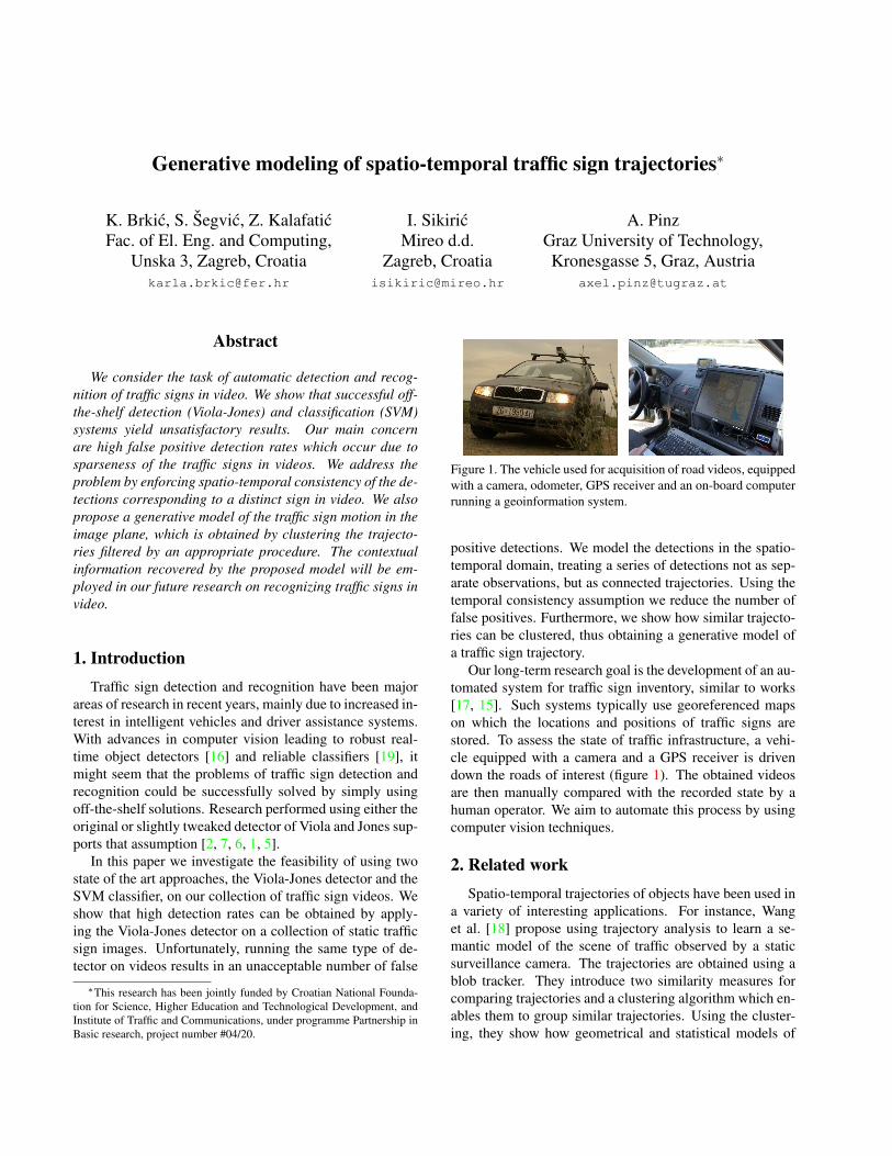
Figure 1. The vehicle used for acquisition of road videos, equipped

with a camera, odometer, GPS receiver and an on-board computer

running a geoinformation system.

positive detections. We model the detections in the spatio-

temporal domain, treating a series of detections not as sep-

arate observations, but as connected trajectories. Using the

temporal consistency assumption we reduce the number of

false positives. Furthermore, we show how similar trajecto-

ries can be clustered, thus obtaining a generative model of

a traffic sign trajectory.

Our long-term research goal is the development of an au-

tomated system for traffic sign inventory, similar to works

[17, 15]. Such systems typically use georeferenced maps

on which the locations and positions of traffic signs are

stored. To assess the state of traffic infrastructure, a vehi-

cle equipped with a camera and a GPS receiver is driven

down the roads of interest (figure 1). The obtained videos

are then manually compared with the recorded state by a

human operator. We aim to automate this process by using

computer vision techniques.

2. Related work

Spatio-temporal trajectories of objects have been used in

a variety of interesting applications. For instance, Wang

et al. [18] propose using trajectory analysis to learn a se-

mantic model of the scene of traffic observed by a static

surveillance camera. The trajectories are obtained using a

blob tracker. They introduce two similarity measures for

comparing trajectories and a clustering algorithm which en-

ables them to group similar trajectories. Using the cluster-

ing, they show how geometrical and statistical models of

the scene can be obtained.

Basharat et al. [3] show how spatio-temporal trajectories

of objects can be used for context-based video matching.

Ricquebourg and Bouthemy [13] employ spatio-

temporal trajectories for real-time tracking of moving per-

sons. The trajectories are built in a predictive model which

enables robust tracking in the case of temporary occlusion.

Khalid and Naftel [10] also use spatio-temporal trajecto-

ries for tracking. The trajectories are not modeled as a set of

points, but as a Fourier series. The coefficients of the series

are used as input feature vectors to a self-organizing map,

which is able to learn the similarities between trajectories in

a non-supervised manner.

Janoos et al. [9] describe the use of spatio-temporal tra-

jectories in detecting anomalous activity.

The research results outlined above encourage us to try

to use trajectory analysis in the context of traffic scenes.

Even though the majority of the existing approaches in tra-

jectory analysis center around a static camera and a moving

object, we believe that traffic scenes are constrained enough

to try to analyze the trajectories obtained by a moving cam-

era. Research on using temporal information for traffic sign

tracking and classification [14, 12] supports that assump-

tion.

3. Using an off-the-shelf solution

To verify the feasibility of using an off-the-shelf solu-

tion for traffic sign detection, we tried two well known ap-

proaches: an object detector proposed by Viola and Jones

[16] and a support vector machine classifier [4]. For train-

ing we used 824 annotated images that contain 898 warning

signs (triangular signs with thick red border), as sometimes

two warning signs appear together. We randomly selected a

total of 10000 negative examples from a set of 100 images

without any traffic signs. For testing we used 344 images

containing 428 signs. The images were drawn from a col-

lection of road videos.

3.1. Applying the Viola­Jones object detector

The object detector proposed by Viola and Jones has

been widely accepted in the computer vision community

in recent years. It works very well, given a reasonable

number of training samples, achieving detection rates up to

95 % [16]. The detector employs a cascade of binary clas-

sifiers obtained by combining multiple Haar-like features in

a boosting framework. The features for each boosted clas-

sifier are selected from a pool by exhaustive search. In the

original paper Discrete AdaBoost is used, but other variants

like LogitBoost, Gentle AdaBoost etc. were also success-

fully applied [11].

The Viola-Jones detector operates by sliding a detection

window across the image and computing the cascade re-

sponse at each position of the detection window. After the

end of the image is reached, the window is enlarged by the

provided scale factor and the process repeats. The precision

and the recall of the detector depend on the scale factor.

In our experiments we used the default resolution of the

detector (i.e. the initial size of the detection window) which

is 24 × 24 pixels. The employed boosting algorithm was

Gentle AdaBoost, as experiments by Lienhart et al. [11] in-

dicate it outperforms other methods. Minimum hit rate was

set to 0.995, and maximum false alarm rate to 0.5 per stage.

20 stages of the cascade were to be trained, however, the

training terminated in stage 17 because required precision

had been reached.

Using scale factor 1.20, the trained detector correctly de-

tected 352 out of 428 traffic signs (82 %). There were 121

false detections. Lowering the scale factor to 1.05 resulted

in the increase of correct detections – 388 signs (90 %) were

detected. However, the number of false positives also in-

creased to 324.

Using a smaller scale factor also lowered the perfor-

mance. The detector processed about 3 images per second

with a scale factor of 1.05, and about 9 images per second

with a scale factor of 1.20 on a quad-core machine. The

resolution of the testing images was 720×576 pixels.

False positive rate might be reduced by adding more pos-

itive and negative examples to the training set. However,

the process of obtaining training images is cumbersome be-

cause it is very time consuming.

3.2. Discriminating true positives using SVM

Observing a large number of false positive detections

obtained by the Viola-Jones detector, we trained a binary

support vector machine classifier. Our intention for it was

to separate true positives from false positives. In train-

ing, we chose a radial basis function kernel K(xi,xj) =exp(−γ)||xi − xj||

2 [8]. We used the images of 898 signs

which were also used for training the Viola-Jones detector,

and 10000 negative images drawn from road scenes without

signs. The training samples were scaled to 20 × 20 pixels.

For each pixel, red, green and blue components were used,

resulting in a sample vector of 1200 elements (20×20 pixels

× 3 color channels).

The penalty parameter C of the SVM was set to 4096.

The γ parameter of the radial basis function was 0.015625.

The values of parameters were obtained by using an exhaus-

tive grid search over a subset of possible parameters. Each

considered pair of parameters was evaluated on the train-

ing set using cross-validation. The pair which produced the

smallest cross-validation error was used.

The SVM classifier was tested on 428 positive examples

and 500 negative examples. The positive examples corre-

sponded to the testing set used for the Viola-Jones detector.

However, the Viola-Jones detector was tested on complete

images, while in the case of the SVM the signs were cut out

from the images, scaled to 20×20 and presented to the clas-

sifier. To test the performance of the classifier of negative

examples, we generated 500 of them by cutting random-

sized patches from images without signs and scaling them

to 20 × 20 pixels.

While the SVM classifier correctly classified all nega-

tives, 23 true positives were misclassified (5 %), indicating

that the classifier is a bit biased towards negatives.

3.3. Experiments with videos

Our target application domain is dependent on videos,

and not on static images. Having obtained promising results

with the Viola-Jones detector on static images, the next log-

ical step was testing it on video data. With the help of an

industrial partner, we obtaned a collection of more than 50

hours of video, acquired mainly on countryside roads and

in small cities. In the videos, signs relevant to the driver

typically occur only on the right side of the road. Roads

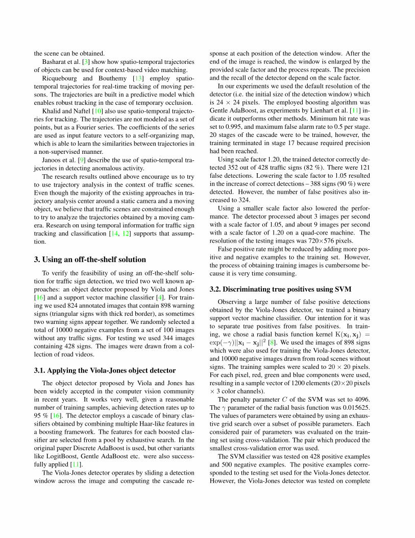
are bidirectional, with one lane for each direction. A few

typical scenes from the videos are shown in figure 2.

Figure 2. A few typical frames taken from our videos.

For our experiments we used three video clips with a

total duration of approximately one hour. Total number of

frames in all three videos was 91335. In the videos a total

of 42 warning signs appeared, which led to a total number

of 1490 frames with signs.

Results obtained by running the Viola-Jones detector

(section 3.1) on videos are summarized in table 1. Over-

all, all the actual signs were detected in at least one frame.

However, the total number of false positives obtained by the

detector was prohibitive. There were 1490 frames which ac-

tually contained signs, and the detector generated 25478 de-

tections. This means that for each actual sign frame we got

more than 15 false detections. It is easy to deduce a cause

for such a large number of false positives: traffic signs in

videos are sparse. In our videos, a traffic sign appears on

average once every 1.4 minutes. One minute of video con-

sists of 1440 frames. The sign will typically be visible and

recognizable in about 50 frames in the optimistic case of the

car driving slowly.

video 1 2 3 all

duration [minutes] 43:08 07:36 10:20 61:04

number of frames 64620 11315 15400 91335

number of signs 26 8 8 42

frames with signs 877 302 311 1490

total detections 18793 3193 3492 25478Table 1. Experimental results for testing the trained Viola-Jones

detector on three different videos.

Having trained the SVM classifier for the purpose of fil-

tering out false positives (section 3.2), we applied it to the

output of the Viola-Jones detector hoping to obtain better

results. There were 23440 detections that SVM classified

as non-signs. Out of those 23440, 440 were true positives.

Considering how sparse true positives are, it is useful to in-

vestigate whether this result could be improved by treating

frames of the video as connected observations, rather than

treating each frame as a separate observation.

4. Adding spatio-temporal constraints

By introducing temporal dependency between frames the

false positive rate of the Viola-Jones detector can be low-

ered considerably. True positives should be temporally con-

sistent between frames. A sign cannot appear in one frame

and disappear in the next. Furthermore, position of a sign

in time changes in a predictable manner, providing useful

cues.

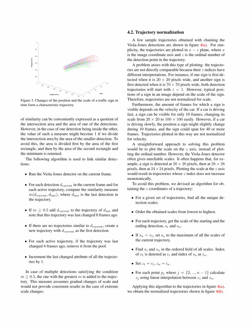
Figure 3 shows the consecutive detections of four dif-

ferent traffic signs during 40 frames. The first detection of

each sign is plotted with z axis coordinate z = 1, the sec-

ond one with z = 2, etc. It can be seen that consecutive

detections form trajectories in the spatio-temporal volume

and that the trajectories of the traffic signs are quite simi-

lar. We will show how these trajectories can be used in the

elimination of false positives and how they can be modeled,

obtaining context in a generative manner.

4.1. Obtaining detection trajectories

The detection chains forming the trajectories are ob-

tained by linking similar detections in consecutive frames.

Given two detection rectangles, d1 and d2, obtained in

consecutive frames, and their intersection dintersect, simi-

larity is computed as follows:

m(d1, d2) = min

(

area(dintersect)

area(d1),area(dintersect)

area(d2)

)

Any measure of similarity between two detections

should take the intersection area into account. The degree

0

10

20

30

400

100

200

300

400

500

600

700

0

100

200

300

400

500

timeimage axis x

ima

ge

axis

y

Figure 3. Changes of the position and the scale of a traffic sign in

time form a characteristic trajectory.

of similarity can be conveniently expressed as a quotient of

the intersection area and the area of one of the detections.

However, in the case of one detection being inside the other,

the value of such a measure might become 1 if we divide

the intersection area by the area of the smaller detection. To

avoid this, the area is divided first by the area of the first

rectangle, and then by the area of the second rectangle and

the minimum is returned.

The following algorithm is used to link similar detec-

tions:

• Run the Viola-Jones detector on the current frame.

• For each detection dcurrent in the current frame and for

each active trajectory, compute the similarity measure

m(dcurrent, dlast), where dlast is the last detection in

the trajectory.

• If m ≥ 0.5 add dcurrent to the trajectory of dlast and

note that this trajectory was last changed 0 frames ago.

• If there are no trajectories similar to dcurrent, create a

new trajectory with dcurrent as the first detection.

• For each active trajectory, if the trajectory was last

changed 4 frames ago, remove it from the pool.

• Increment the last changed attribute of all the trajecto-

ries by 1.

In case of multiple detections satisfying the condition

m ≥ 0.5, the one with the greatest m is added to the trajec-

tory. This measure asssumes gradual changes of scale and

would not provide consistent results in the case of extreme

scale changes.

4.2. Trajectory normalization

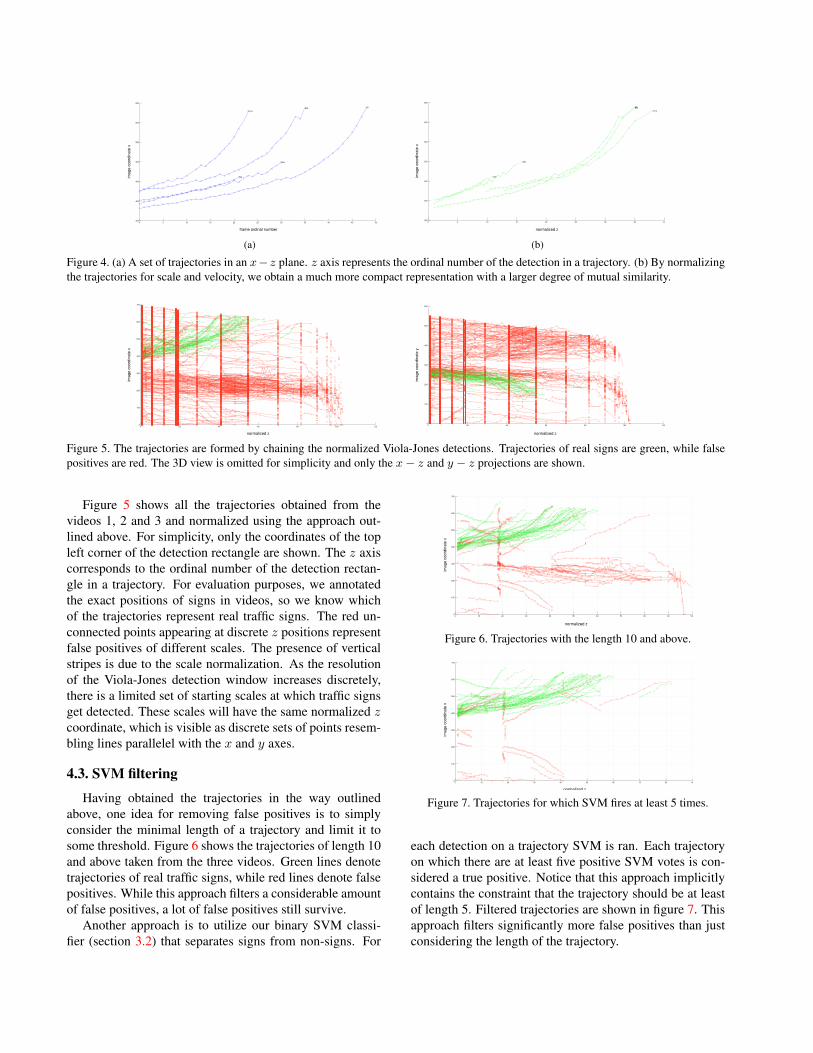
A few sample trajectories obtained with chaining the

Viola-Jones detections are shown in figure 4(a). For sim-

plicity, the trajectories are plotted in x − z plane, where x

is the image coordinate axis and z is the ordinal number of

the detection point in the trajectory.

A problem arises with this type of plotting: the trajecto-

ries are not directly comparable because their z indices have

different interpretations. For instance, if one sign is first de-

tected when it is 20 × 20 pixels wide, and another sign is

first detected when it is 70 × 70 pixels wide, both detection

trajectories will start with z = 1. However, typical posi-

tions of a sign in an image depend on the scale of the sign.

Therefore, trajectories are not normalized for scale.

Furthermore, the amount of frames for which a sign is

visible depends on the velocity of the car. If a car is driving

fast, a sign can be visible for only 10 frames, changing its

scale from 20 × 20 to 100 × 100 easily. However, if a car

is driving slowly, the position a sign might slightly change

during 10 frames, and the sign could span for 40 or more

frames. Trajectories plotted in this way are not normalized

for velocity.

A straightforward approach to solving this problem

would be to plot the scale on the z axis, instead of plot-

ting the ordinal number. However, the Viola-Jones detector

often gives unreliable scales. It often happens that, for ex-

ample, a sign is detected at 20 × 20 pixels, then at 28 × 28pixels, then at 24×24 pixels. Plotting the scale at the z axis

would result in trajectories whose z index does not increase

monotonically.

To avoid this problem, we devised an algorithm for ob-

taining the z coordinates of a trajectory:

• For a given set of trajectories, find all the unique de-

tection scales.

• Order the obtained scales from lowest to highest.

• For each trajectory, get the scale of the starting and the

ending detection, s1 and sn.

• If sn = s1, set sn to the maximum of all the scales of

the current trajectory.

• Find s1 and sn in the ordered field of all scales. Index

of s1 is denoted as i1 and index of sn as in.

• Set z1 = i1, zn = in.

• For each point pj where j = {2, ..., n − 1} calculate

zj using linear interpolation between z1 and zn.

Applying this algorithm to the trajectories in figure 4(a),

we obtain the normalized trajectories shown in figure 4(b).

0 5 10 15 20 25 30 35 40 45 50350

400

450

500

550

600

650

20826

684

frame ordinal number

1210

730ima

ge

co

ord

ina

te x

(a)

0 5 10 15 20 25 30 35 40350

400

450

500

550

600

650

1210

20826

normalized z

684

730ima

ge

co

ord

ina

te x

(b)

Figure 4. (a) A set of trajectories in an x− z plane. z axis represents the ordinal number of the detection in a trajectory. (b) By normalizing

the trajectories for scale and velocity, we obtain a much more compact representation with a larger degree of mutual similarity.

0 20 40 60 80 100 1200

100

200

300

400

500

600

700

normalized z

image c

oord

inate

x

0 20 40 60 80 100 1200

100

200

300

400

500

600

normalized z

image c

oord

inate

y

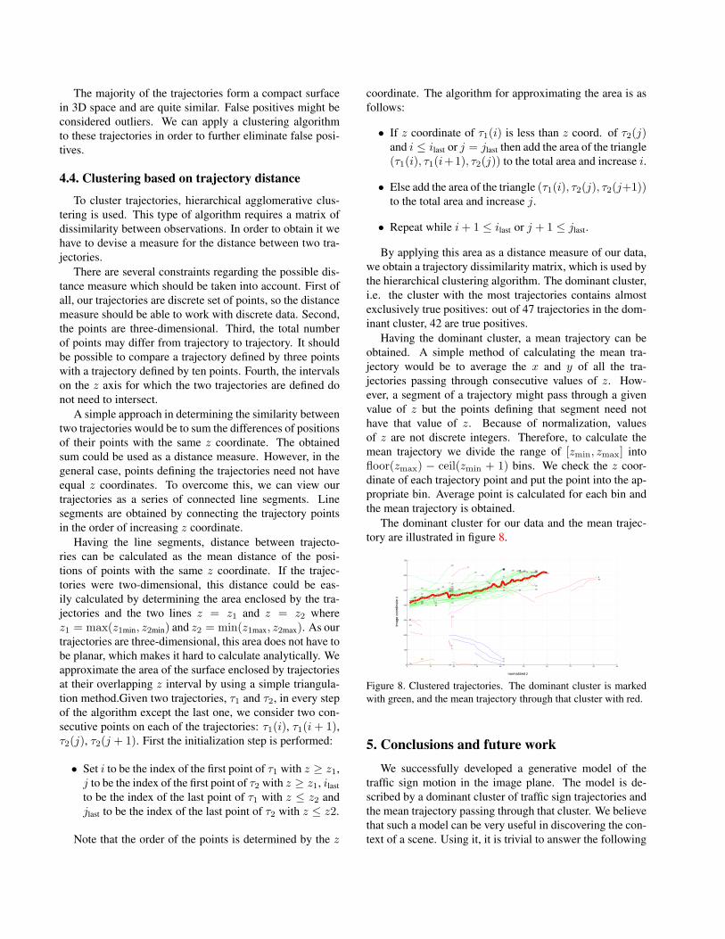
Figure 5. The trajectories are formed by chaining the normalized Viola-Jones detections. Trajectories of real signs are green, while false

positives are red. The 3D view is omitted for simplicity and only the x− z and y − z projections are shown.

Figure 5 shows all the trajectories obtained from the

videos 1, 2 and 3 and normalized using the approach out-

lined above. For simplicity, only the coordinates of the top

left corner of the detection rectangle are shown. The z axis

corresponds to the ordinal number of the detection rectan-

gle in a trajectory. For evaluation purposes, we annotated

the exact positions of signs in videos, so we know which

of the trajectories represent real traffic signs. The red un-

connected points appearing at discrete z positions represent

false positives of different scales. The presence of vertical

stripes is due to the scale normalization. As the resolution

of the Viola-Jones detection window increases discretely,

there is a limited set of starting scales at which traffic signs

get detected. These scales will have the same normalized z

coordinate, which is visible as discrete sets of points resem-

bling lines parallelel with the x and y axes.

4.3. SVM filtering

Having obtained the trajectories in the way outlined

above, one idea for removing false positives is to simply

consider the minimal length of a trajectory and limit it to

some threshold. Figure 6 shows the trajectories of length 10

and above taken from the three videos. Green lines denote

trajectories of real traffic signs, while red lines denote false

positives. While this approach filters a considerable amount

of false positives, a lot of false positives still survive.

Another approach is to utilize our binary SVM classi-

fier (section 3.2) that separates signs from non-signs. For

0 10 20 30 40 50 60 70 80 90 1000

100

200

300

400

500

600

700

normalized z

image c

oord

inate

x

Figure 6. Trajectories with the length 10 and above.

0 10 20 30 40 50 60 70 80 900

100

200

300

400

500

600

700

normalized z

ima

ge

co

ord

ina

te x

Figure 7. Trajectories for which SVM fires at least 5 times.

each detection on a trajectory SVM is ran. Each trajectory

on which there are at least five positive SVM votes is con-

sidered a true positive. Notice that this approach implicitly

contains the constraint that the trajectory should be at least

of length 5. Filtered trajectories are shown in figure 7. This

approach filters significantly more false positives than just

considering the length of the trajectory.

The majority of the trajectories form a compact surface

in 3D space and are quite similar. False positives might be

considered outliers. We can apply a clustering algorithm

to these trajectories in order to further eliminate false posi-

tives.

4.4. Clustering based on trajectory distance

To cluster trajectories, hierarchical agglomerative clus-

tering is used. This type of algorithm requires a matrix of

dissimilarity between observations. In order to obtain it we

have to devise a measure for the distance between two tra-

jectories.

There are several constraints regarding the possible dis-

tance measure which should be taken into account. First of

all, our trajectories are discrete set of points, so the distance

measure should be able to work with discrete data. Second,

the points are three-dimensional. Third, the total number

of points may differ from trajectory to trajectory. It should

be possible to compare a trajectory defined by three points

with a trajectory defined by ten points. Fourth, the intervals

on the z axis for which the two trajectories are defined do

not need to intersect.

A simple approach in determining the similarity between

two trajectories would be to sum the differences of positions

of their points with the same z coordinate. The obtained

sum could be used as a distance measure. However, in the

general case, points defining the trajectories need not have

equal z coordinates. To overcome this, we can view our

trajectories as a series of connected line segments. Line

segments are obtained by connecting the trajectory points

in the order of increasing z coordinate.

Having the line segments, distance between trajecto-

ries can be calculated as the mean distance of the posi-

tions of points with the same z coordinate. If the trajec-

tories were two-dimensional, this distance could be eas-

ily calculated by determining the area enclosed by the tra-

jectories and the two lines z = z1 and z = z2 where

z1 = max(z1min, z2min) and z2 = min(z1max, z2max). As our

trajectories are three-dimensional, this area does not have to

be planar, which makes it hard to calculate analytically. We

approximate the area of the surface enclosed by trajectories

at their overlapping z interval by using a simple triangula-

tion method.Given two trajectories, τ1 and τ2, in every step

of the algorithm except the last one, we consider two con-

secutive points on each of the trajectories: τ1(i), τ1(i + 1),τ2(j), τ2(j + 1). First the initialization step is performed:

• Set i to be the index of the first point of τ1 with z ≥ z1,

j to be the index of the first point of τ2 with z ≥ z1, ilast

to be the index of the last point of τ1 with z ≤ z2 and

jlast to be the index of the last point of τ2 with z ≤ z2.

Note that the order of the points is determined by the z

coordinate. The algorithm for approximating the area is as

follows:

• If z coordinate of τ1(i) is less than z coord. of τ2(j)and i ≤ ilast or j = jlast then add the area of the triangle

(τ1(i), τ1(i+1), τ2(j)) to the total area and increase i.

• Else add the area of the triangle (τ1(i), τ2(j), τ2(j+1))to the total area and increase j.

• Repeat while i + 1 ≤ ilast or j + 1 ≤ jlast.

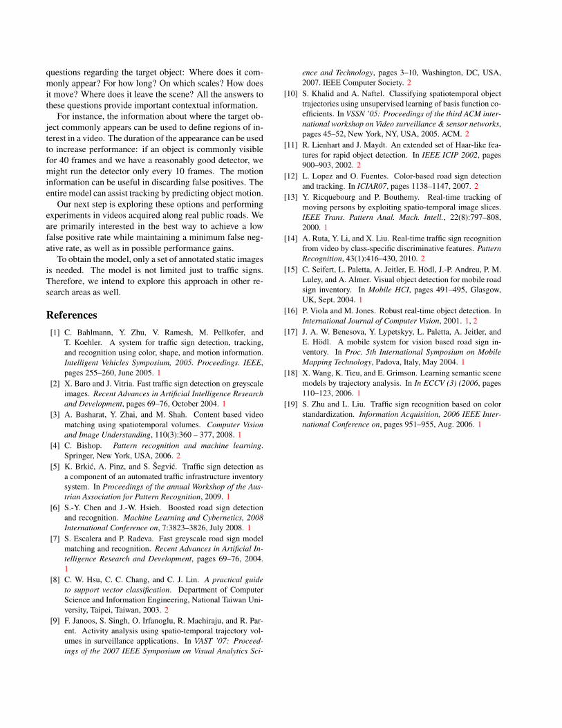
By applying this area as a distance measure of our data,

we obtain a trajectory dissimilarity matrix, which is used by

the hierarchical clustering algorithm. The dominant cluster,

i.e. the cluster with the most trajectories contains almost

exclusively true positives: out of 47 trajectories in the dom-

inant cluster, 42 are true positives.

Having the dominant cluster, a mean trajectory can be

obtained. A simple method of calculating the mean tra-

jectory would be to average the x and y of all the tra-

jectories passing through consecutive values of z. How-

ever, a segment of a trajectory might pass through a given

value of z but the points defining that segment need not

have that value of z. Because of normalization, values

of z are not discrete integers. Therefore, to calculate the

mean trajectory we divide the range of [zmin, zmax] into

floor(zmax) − ceil(zmin + 1) bins. We check the z coor-

dinate of each trajectory point and put the point into the ap-

propriate bin. Average point is calculated for each bin and

the mean trajectory is obtained.

The dominant cluster for our data and the mean trajec-

tory are illustrated in figure 8.

0 10 20 30 40 50 60 70 80 900

100

200

300

400

500

600

700

8

23

202020

20

20

20

20

20

202020202020202020

1820

20

20

normalized z

20202020

21

20

14

12

2020

21

20

21

2019

20

1

6

20

20

20

5

20

3

20

2020

10

20

20

20

4

20

20

20

2020

22

20

20

2

20

20

20

20

20

20

1620

20

20

20

20

20

22

20

7

20

2020

20

11

13

9

15

17

ima

ge

co

ord

ina

te x

Figure 8. Clustered trajectories. The dominant cluster is marked

with green, and the mean trajectory through that cluster with red.

5. Conclusions and future work

We successfully developed a generative model of the

traffic sign motion in the image plane. The model is de-

scribed by a dominant cluster of traffic sign trajectories and

the mean trajectory passing through that cluster. We believe

that such a model can be very useful in discovering the con-

text of a scene. Using it, it is trivial to answer the following

questions regarding the target object: Where does it com-

monly appear? For how long? On which scales? How does

it move? Where does it leave the scene? All the answers to

these questions provide important contextual information.

For instance, the information about where the target ob-

ject commonly appears can be used to define regions of in-

terest in a video. The duration of the appearance can be used

to increase performance: if an object is commonly visible

for 40 frames and we have a reasonably good detector, we

might run the detector only every 10 frames. The motion

information can be useful in discarding false positives. The

entire model can assist tracking by predicting object motion.

Our next step is exploring these options and performing

experiments in videos acquired along real public roads. We

are primarily interested in the best way to achieve a low

false positive rate while maintaining a minimum false neg-

ative rate, as well as in possible performance gains.

To obtain the model, only a set of annotated static images

is needed. The model is not limited just to traffic signs.

Therefore, we intend to explore this approach in other re-

search areas as well.

References

[1] C. Bahlmann, Y. Zhu, V. Ramesh, M. Pellkofer, and

T. Koehler. A system for traffic sign detection, tracking,

and recognition using color, shape, and motion information.

Intelligent Vehicles Symposium, 2005. Proceedings. IEEE,

pages 255–260, June 2005. 1

[2] X. Baro and J. Vitria. Fast traffic sign detection on greyscale

images. Recent Advances in Artificial Intelligence Research

and Development, pages 69–76, October 2004. 1

[3] A. Basharat, Y. Zhai, and M. Shah. Content based video

matching using spatiotemporal volumes. Computer Vision

and Image Understanding, 110(3):360 – 377, 2008. 1

[4] C. Bishop. Pattern recognition and machine learning.

Springer, New York, USA, 2006. 2

[5] K. Brkic, A. Pinz, and S. Segvic. Traffic sign detection as

a component of an automated traffic infrastructure inventory

system. In Proceedings of the annual Workshop of the Aus-

trian Association for Pattern Recognition, 2009. 1

[6] S.-Y. Chen and J.-W. Hsieh. Boosted road sign detection

and recognition. Machine Learning and Cybernetics, 2008

International Conference on, 7:3823–3826, July 2008. 1

[7] S. Escalera and P. Radeva. Fast greyscale road sign model

matching and recognition. Recent Advances in Artificial In-

telligence Research and Development, pages 69–76, 2004.

1

[8] C. W. Hsu, C. C. Chang, and C. J. Lin. A practical guide

to support vector classification. Department of Computer

Science and Information Engineering, National Taiwan Uni-

versity, Taipei, Taiwan, 2003. 2

[9] F. Janoos, S. Singh, O. Irfanoglu, R. Machiraju, and R. Par-

ent. Activity analysis using spatio-temporal trajectory vol-

umes in surveillance applications. In VAST ’07: Proceed-

ings of the 2007 IEEE Symposium on Visual Analytics Sci-

ence and Technology, pages 3–10, Washington, DC, USA,

2007. IEEE Computer Society. 2

[10] S. Khalid and A. Naftel. Classifying spatiotemporal object

trajectories using unsupervised learning of basis function co-

efficients. In VSSN ’05: Proceedings of the third ACM inter-

national workshop on Video surveillance & sensor networks,

pages 45–52, New York, NY, USA, 2005. ACM. 2

[11] R. Lienhart and J. Maydt. An extended set of Haar-like fea-

tures for rapid object detection. In IEEE ICIP 2002, pages

900–903, 2002. 2

[12] L. Lopez and O. Fuentes. Color-based road sign detection

and tracking. In ICIAR07, pages 1138–1147, 2007. 2

[13] Y. Ricquebourg and P. Bouthemy. Real-time tracking of

moving persons by exploiting spatio-temporal image slices.

IEEE Trans. Pattern Anal. Mach. Intell., 22(8):797–808,

2000. 1

[14] A. Ruta, Y. Li, and X. Liu. Real-time traffic sign recognition

from video by class-specific discriminative features. Pattern

Recognition, 43(1):416–430, 2010. 2

[15] C. Seifert, L. Paletta, A. Jeitler, E. Hodl, J.-P. Andreu, P. M.

Luley, and A. Almer. Visual object detection for mobile road

sign inventory. In Mobile HCI, pages 491–495, Glasgow,

UK, Sept. 2004. 1

[16] P. Viola and M. Jones. Robust real-time object detection. In

International Journal of Computer Vision, 2001. 1, 2

[17] J. A. W. Benesova, Y. Lypetskyy, L. Paletta, A. Jeitler, and

E. Hodl. A mobile system for vision based road sign in-

ventory. In Proc. 5th International Symposium on Mobile

Mapping Technology, Padova, Italy, May 2004. 1

[18] X. Wang, K. Tieu, and E. Grimson. Learning semantic scene

models by trajectory analysis. In In ECCV (3) (2006, pages

110–123, 2006. 1

[19] S. Zhu and L. Liu. Traffic sign recognition based on color

standardization. Information Acquisition, 2006 IEEE Inter-

national Conference on, pages 951–955, Aug. 2006. 1