![PEP Web - The Analytic Third: Working with Intersubjective ... … · analytic third'. This third subjectivity, the intersubjective analytic third Green's [1975] 'analytic object'),](https://static.fdocuments.us/doc/165x107/6099619e2d4b51336024f694/pep-web-the-analytic-third-working-with-intersubjective-analytic-third.jpg)
Generating Trading Agent Strategies: Analytic and ...
165
Generating Trading Agent Strategies: Analytic and Empirical Methods for Infinite and Large Games by Daniel M. Reeves A dissertation submitted in partial fulfillment of the requirements for the degree of Doctor of Philosophy (Computer Science and Engineering) in The University of Michigan 2005 Doctoral Committee: Professor Michael P. Wellman, Chair Professor Jeffrey K. MacKie-Mason Professor Scott E. Page Associate Professor Satinder Singh Baveja
Transcript of Generating Trading Agent Strategies: Analytic and ...

Generating Trading Agent Strategies:Analytic and Empirical Methods
for Infinite and Large Games
by
Daniel M. Reeves
A dissertation submitted in partial fulfillmentof the requirements for the degree of
Doctor of Philosophy(Computer Science and Engineering)
in The University of Michigan2005
Doctoral Committee:Professor Michael P. Wellman, ChairProfessor Jeffrey K. MacKie-MasonProfessor Scott E. PageAssociate Professor Satinder Singh Baveja

First edition
c© 2005 by Daniel M. Reeves
Artificial Intelligence LaboratoryUniversity of Michigan1101 Beal AvenueAnn Arbor, Michigan, 48109USA
http://ai.eecs.umich.edu/people/dreeves

To my parents, Laurie Kalkman Reeves and Martin Reeves.


Abstract
A Strategy Generation Engine is a system that reads a description of a game or market mechanismand outputs strategies for participants. Ideally, this means a game solver—an algorithm to computeNash equilibria. This is a well-studied problem and very general solutions exist, but they can onlybe applied to small, finite games. This thesis presents methods for finding or approximating Nashequilibria for infinite games, and for intractably large finite games.
First, I define a broad class of one-shot, two-player infinite games of incomplete information.I present an algorithm for computing best-response strategies in this class and show that for manyparticular games the algorithm can be iterated to compute Nash equilibria. Many results from thegame theory literature are reproduced—automatically—using this method, as well as novel resultsfor new games.
Next, I address the problem of finding strategies in games that, even if finite, are larger than whatany exact solution method can address. Our solution involves (1) generating a small set of candidatestrategies, (2) constructing via simulation an approximate payoff matrix for the simplification of thegame restricted to the candidate strategies, (3) analyzing the empirical game, and (4) assessingthe quality of solutions with respect to the underlying full game. I leave methods for generatingcandidate strategies domain-specific and focus on methods for taming the computational cost ofempirical game generation. I do this by employing Monte Carlo variance reduction techniques andintroducing a technique for approximating many-player games by reducing the number of players.We are additionally able to solve much larger payoff matrices than the current state-of-the-art solverby exploiting symmetry in games.
I test these methods in small games with known solutions and then apply them to two realisticmarket scenarios: Simultaneous Ascending Auctions (SAA) and the Trading Agent Competition(TAC) travel-shopping game. For these domains I focus on two key price prediction approachesfor generating candidate strategies for empirical analysis: self-confirming price predictions andWalrasian equilibrium prices. We find that these are highly effective strategies in SAA and TAC,respectively.
v


Acknowledgments
This thesis includes joint work with Michael Wellman, Jeffrey MacKie-Mason, Anna Osepayshvili,Kevin Lochner, Shih-Fen Cheng, Rahul Suri, Yevgeniy Vorobeychik, and Maxim Rytin. In Sec-tion 1.4 I outline this thesis in relation to previously published work with the above coauthors. Mycollaboration with Maxim Rytin, though, is published here for the first time as the proofs of keytheorems in Chapter 3. Kevin O’Malley was instrumental in the development of our entry in theTrading Agent Competition, which is the subject of Chapter 6. Finally, William Walsh collaboratedon the proofs of theorems related to the supply-chain game in Chapter 2.
I’m grateful to my thesis committee—Michael Wellman, Jeffrey MacKie-Mason, Scott Page,and Satinder Singh Baveja—for their careful reading, insightful comments, and cutting questions.This thesis is definitively improved due to their input. As early as my proposal defense, Satinderhelped shape the course of this research by proposing what led to our epsilon metric, defined inChapter 3. Similarly, Scott has proposed myriad improvements and helped clarify the contributionin Chapter 2 by asking hard questions about the generality of my approach. Even before Scott cameto Michigan, he provided invaluable guidance at the Computational Economics Workshop at theSanta Fe Institute in 2000, when I first got excited about strategy generation in auctions. Jeff, ofcourse, is much more than a committee member. As a coauthor of most of the material in Chapters 3,4, and 5, it’s thanks in no small part to his vision and hard work that this thesis is where it is.
This brings me to Mike. Perhaps it’s filial bias but I am convinced there is no better researchadvisor in all of academia. Mike’s research and thesis advising is nothing short of a graduatestudent’s dream. He is an academic role model in every way, and I just can’t thank him enoughfor his guidance and patience. Guidance doesn’t capture it—he was a full collaborator (includingwriting code, running experiments, and proving theorems) on everything in this thesis. Patience islikewise an understatement; if he was ever frustrated by my almost explicit goal of stretching mygraduate school career out as long as possible, he didn’t let on. I also won’t forget how kind he waswhen I was ill in 2002.
Others who I would like to thank for their help, support, or guidance include Terence Kelly, An-drzej Kozlowski, Daniel Lichtblau, Ted Turocy, Benjamin Grosof, David Reiley, Leslie Fine, Kay-yut Chen, Jaap Suermondt, Evan Kirshenbaum, Kemal Guler, John Miller, Annie Noone, BethanySoule, Dave Morris, Chris Kapusky, Karen Conneely, Sarah Nuss-Warren, Rachel Rose, Rob Felty,Michelle Sternthal, Doug Bryan, Brian Renaud, Marie Eguchi, and finally, my family.
vii


Contents
1 Introduction: Games, Strategies, and Nash Equilibria 11.1 Games of Incomplete Information and Normal-Form Representation . . . . . . . . 11.2 Symmetric Games . . . . . . . . . . . . . . . . . . . . . . . . . . . . . . . . . . . 31.3 Summary and Motivation . . . . . . . . . . . . . . . . . . . . . . . . . . . . . . . 31.4 Overview of Thesis . . . . . . . . . . . . . . . . . . . . . . . . . . . . . . . . . . 5
2 Generating Best-Response Strategies in Infinite Games of Incomplete Information 72.1 Finite Game Approximations . . . . . . . . . . . . . . . . . . . . . . . . . . . . . 72.2 Infinite Games and Bayes-Nash Equilibria . . . . . . . . . . . . . . . . . . . . . . 82.3 Existence and Computation of Piecewise Linear Best-Response Strategies . . . . . 112.4 Examples . . . . . . . . . . . . . . . . . . . . . . . . . . . . . . . . . . . . . . . 132.5 Related Work . . . . . . . . . . . . . . . . . . . . . . . . . . . . . . . . . . . . . 18
3 Empirical Game Methodology 213.1 Measuring Solution Quality: The ε Metric . . . . . . . . . . . . . . . . . . . . . . 223.2 Restricting the Strategy Space . . . . . . . . . . . . . . . . . . . . . . . . . . . . 233.3 Game Simulators and Brute-Force Estimation of Games . . . . . . . . . . . . . . . 263.4 Variance Reduction in Monte Carlo Sampling . . . . . . . . . . . . . . . . . . . . 283.5 Reducing the Number of Players . . . . . . . . . . . . . . . . . . . . . . . . . . . 323.6 Analyzing Empirical Games . . . . . . . . . . . . . . . . . . . . . . . . . . . . . 373.7 Interleaving Analysis and Estimation . . . . . . . . . . . . . . . . . . . . . . . . . 403.8 Sensitivity Analysis . . . . . . . . . . . . . . . . . . . . . . . . . . . . . . . . . . 413.9 Related Work . . . . . . . . . . . . . . . . . . . . . . . . . . . . . . . . . . . . . 43
4 Price Prediction for Strategy Generation in Complex Market Mechanisms 474.1 Interdependent Auctions: TAC and SAA . . . . . . . . . . . . . . . . . . . . . . . 474.2 Walrasian Price Equilibrium . . . . . . . . . . . . . . . . . . . . . . . . . . . . . 484.3 The Simultaneous Ascending Auctions (SAA) Domain . . . . . . . . . . . . . . . 504.4 Strategies for SAA: Straightforward Bidding and Variations . . . . . . . . . . . . . 514.5 Price Prediction Strategies for SAA . . . . . . . . . . . . . . . . . . . . . . . . . 544.6 Methods for Predicting Prices in SAA . . . . . . . . . . . . . . . . . . . . . . . . 574.7 The Trading Agent Competition (TAC) Domain . . . . . . . . . . . . . . . . . . . 594.8 Price Prediction in TAC . . . . . . . . . . . . . . . . . . . . . . . . . . . . . . . . 614.9 Walrasian Price Equilibrium in the TAC Market . . . . . . . . . . . . . . . . . . . 614.10 Bidding Strategy using Price Predictions in TAC . . . . . . . . . . . . . . . . . . . 664.11 Evaluating Prediction Quality in TAC . . . . . . . . . . . . . . . . . . . . . . . . 68
ix

x CONTENTS
4.12 Conclusion . . . . . . . . . . . . . . . . . . . . . . . . . . . . . . . . . . . . . . 70
5 Empirical Game Analysis for Simultaneous Ascending Auctions 735.1 Type Distributions for SAA . . . . . . . . . . . . . . . . . . . . . . . . . . . . . . 735.2 Experiments in Sunk-Awareness . . . . . . . . . . . . . . . . . . . . . . . . . . . 755.3 Sensitivity Analysis for Sunk-Awareness Results . . . . . . . . . . . . . . . . . . 815.4 Baseline Price Prediction vs. Straightforward Bidding . . . . . . . . . . . . . . . . 825.5 How Does Price Prediction Help? . . . . . . . . . . . . . . . . . . . . . . . . . . 865.6 Comparison of Point Predictors . . . . . . . . . . . . . . . . . . . . . . . . . . . . 885.7 Self-Confirming Distribution Predictors . . . . . . . . . . . . . . . . . . . . . . . 895.8 Conclusion . . . . . . . . . . . . . . . . . . . . . . . . . . . . . . . . . . . . . . 93
6 Taming TAC: Searching for Walverine 956.1 Preliminary Strategic Analysis: Shading vs. Non-Shading . . . . . . . . . . . . . . 956.2 Walverine Parameters . . . . . . . . . . . . . . . . . . . . . . . . . . . . . . . . . 976.3 Control Variates for the TAC Game . . . . . . . . . . . . . . . . . . . . . . . . . . 1006.4 Player-Reduced TAC Experiments . . . . . . . . . . . . . . . . . . . . . . . . . . 1026.5 Finding Walverine 2005 . . . . . . . . . . . . . . . . . . . . . . . . . . . . . . . . 1116.6 TAC 2005 Outcome . . . . . . . . . . . . . . . . . . . . . . . . . . . . . . . . . . 1126.7 Related Work: Strategic Interactions in TAC Travel . . . . . . . . . . . . . . . . . 114
7 Conclusion 1177.1 Summary of Contribution . . . . . . . . . . . . . . . . . . . . . . . . . . . . . . . 1177.2 Future Work . . . . . . . . . . . . . . . . . . . . . . . . . . . . . . . . . . . . . . 119
A Proofs and Derivations 121A.1 CDF of a Piecewise Uniform Distribution . . . . . . . . . . . . . . . . . . . . . . 121A.2 Proof of Theorem 2.3 . . . . . . . . . . . . . . . . . . . . . . . . . . . . . . . . . 121A.3 Proof of Theorem 2.4 . . . . . . . . . . . . . . . . . . . . . . . . . . . . . . . . . 122A.4 Proof of Theorem 2.5 . . . . . . . . . . . . . . . . . . . . . . . . . . . . . . . . . 124A.5 Proof of Theorem 3.4 . . . . . . . . . . . . . . . . . . . . . . . . . . . . . . . . . 124A.6 Proof of Theorem 3.5 . . . . . . . . . . . . . . . . . . . . . . . . . . . . . . . . . 126A.7 Proof of Lemma 3.7 . . . . . . . . . . . . . . . . . . . . . . . . . . . . . . . . . . 127A.8 Proof of Theorem 3.10 . . . . . . . . . . . . . . . . . . . . . . . . . . . . . . . . 129A.9 Proof of Lemma 3.11 . . . . . . . . . . . . . . . . . . . . . . . . . . . . . . . . . 130A.10 Proof of Theorem 3.12 . . . . . . . . . . . . . . . . . . . . . . . . . . . . . . . . 131A.11 Proof of Theorem 3.13 . . . . . . . . . . . . . . . . . . . . . . . . . . . . . . . . 131
B Monte Carlo Best-Response Estimation 133
C Notes on Equilibria in Symmetric Games 135
D Strategies for SAA Experiments 139D.1 Price Predicting Strategies . . . . . . . . . . . . . . . . . . . . . . . . . . . . . . 139D.2 53-Strategy Game For 5×5 Uniform Environment . . . . . . . . . . . . . . . . . . 143D.3 Strategies For Alternative Environments . . . . . . . . . . . . . . . . . . . . . . . 144
Bibliography 147

Chapter 1
Introduction: Games, Strategies, and NashEquilibria
IN WHICH we define terms like “game” and “strategy” and introduce the problem ofgenerating strategies for games.
When a human is faced with a new game they digest the rules, consider the motives and ca-pabilities of the other players, and formulate a strategy for playing. This thesis takes steps towardautomating that process. A Strategy Generation Engine is a system that advises on how to play agame given a formal description of the possible interactions of the players. In the absence of otherplayers, a strategy generation engine is just an optimization routine. That is, it would answer, deci-sion theoretically, the question: What actions maximize my (expected) utility? In the next section,we see how, by way of a cursory introduction to some foundational concepts of game theory, thestrategy generation concept can be generalized to the case of multiple agents: a game.
1.1 Games of Incomplete Information and Normal-Form Representation
Game theory was founded by von Neumann and Morgenstern [1947] to study situations in whichmultiple agents (players) interact in order to each maximize an objective (payoff) function deter-mined not only by their own actions but also the actions of other players. Agents always knowtheir own payoff function—i.e., their utility function—but may not know those of the other agents.To capture this, we redefine an agent’s payoff to be a function not only of its own and others’ ac-tions, but also of private information. Thus it is without loss of generality to consider all the payofffunctions (or, equivalently, the single multidimensional payoff function) as known by all the agents.
An agent’s private information is known more succinctly as its type, or sometimes as its pref-erences. The term “type” is used because it is exactly this private information that formally distin-guishes the agents. The term “preferences” reflects the fact that the private information determinesthe agent’s utility, given all the agents’ actions. For example, in poker an agent’s hand constitutes itstype. In an auction, the analogous information is how much the agent values the goods being sold.
The agents’ types are drawn from a probability distribution, called the type distribution. Tocapture randomness in the game, we introduce a special player, Nature, with type dictated, as forany other player, by the type distribution. But Nature has no payoff function and its action is simplyits type. In this way Nature could, for example, represent the roll of dice, affecting any or all
1

2 CHAPTER 1. INTRODUCTION
other players’ payoffs. We assume that the possible actions, payoff function, and type distributionare common knowledge.1 The special case that all agents have exactly one possible type is calledcomplete information. In this thesis, I consider the general case: games of incomplete information.
Nash Equilibrium
In the case of a single agent, the optimal policy is straightforward: choose the action that maximizespayoff (utility). If payoff depends on Nature’s action, the agent simply maximizes its expectedpayoff given the type distribution. In the case of multiple agents, Nash [1951] proposed a solutionconcept now known as the Nash equilibrium and proved that for finite games (as long as agents canplay mixed strategies, i.e., randomize among actions) such an equilibrium always exists. A Nashequilibrium that does not employ mixed strategies—called a pure-strategy Nash equilibrium—is aprofile of actions such that each action is a best response to the rest of the profile. That is, eachagent maximizes its own utility given the actions played by the others. The generalization to mixed-strategy equilibria entails maximizing expected utility given the distribution of agent actions.
Although the limitations of the Nash equilibrium as a solution concept have been well studied,particularly the problem of what agents will do in the face of multiple equilibria [van Damme, 1983],finding Nash equilibria remains fundamental to the analysis of games. In fact, for many practicalapplications, it suffices to find one of many possible Nash equilibria. That equilibrium, by virtueof being the one found by a given solver, becomes focal and the equilibrium selection problemis moot. For example, if agent software is distributed that implements an equilibrium policy fora game, no recipient has an incentive to modify the software unless they imagine that others arealso modifying it in a certain way, which they would have no incentive to do. Practically, this isreasonable assurance the found equilibrium will actually be played.
Bayes-Nash Equilibrium
The notion of Nash equilibrium needs to be generalized slightly for the case of incomplete in-formation games. We first define an agent’s strategy as a mapping from its information—privateinformation (type) as well as information revealed during the game—to actions. Another seminalgame theorist, Harsanyi2 [1967], first introduced the concept of agent types and used it to define aBayesian game. A Bayesian game is specified by a set of types T , a set of actions A, a probabilitydistribution F over types, and a payoff function P . Harsanyi defines a Bayes-Nash equilibrium(sometimes known as a Bayesian equilibrium) as the simple Nash equilibrium of the non-Bayesiangame with set of actions being the set of strategies (functions from T to A), and the payoff functionbeing the expectation of P with respect to F . In this thesis I use “Nash equilibrium” or “equilib-rium” interchangeably with “Bayes-Nash equilibrium” when appropriate.
The idea of a normal (or strategic) form representation is to ignore the actions and define thegame in terms of the strategies. In other words, per Harsanyi’s insight, an agent’s set of strategies isequivalent to its set of actions.
Definition 1.1 (Normal-form Game) Γ = 〈n, {Si}, {ui()}〉 is an n-player normal-form game,with strategy set Si the available strategies for player i (with typical element si), and the payoff
1A fact is common knowledge [Fagin et al., 1995] if everyone knows it, everyone knows that everyone knows it, adinfinitum.
2Harsanyi, along with Selten, shared the 1994 Nobel Prize in economics with Nash “for their pioneering analysis ofequilibria in the theory of non-cooperative games.”

1.2. SYMMETRIC GAMES 3
function ui(s1, . . . , sn) giving the utility accruing to player i when players choose the strategyprofile (s1, . . . , sn).
In contrast, extensive form is a more compact representation in which payoffs are given for se-quences of actions but only implicitly for combinations of agent strategies (mappings from infor-mation to actions).
1.2 Symmetric Games
With the exception of the bargaining game in Section 2.4, every game I examine in this thesis issymmetric. A game in normal form is symmetric if all agents have the same strategy set, and thepayoff to playing a given strategy depends only on the strategies being played, not on who playsthem. In other words, a game is symmetric if there are no distinct player roles or identities (asidefrom Nature). I define this concept formally as follows:
Definition 1.2 (Symmetric Game) A normal-form game is symmetric if the players have identicalstrategy spaces (S1 = . . . = Sn = S) and ui(si, s−i) = uj(sj , s−j), for si = sj and s−i = s−j
for all i, j ∈ {1, . . . , n}.3 Thus we can write u(t, s) for the payoff to any player playing strategy twhen the remaining players play profile s. We denote a symmetric game by the tuple 〈n, S, u()〉. (Ioverload S to refer to the number of strategies as well as the set of strategies.)
A strategy profile with all players playing the same strategy is a symmetric profile, or, if such aprofile is a Nash equilibrium, a symmetric equilibrium.
Many well-known games are symmetric, for example the Prisoners’ Dilemma, Chicken, andRock-Paper-Scissors, as well as standard game-theoretic auction models. Symmetric games maynaturally arise from models of automated-agent interactions, since in these environments the agentsmay possess, by design, identical circumstances, capabilities, and perspectives. But these are en-compassed in the agent types so even if they differ it is often accurate to model them as drawnfrom identical distributions, restoring symmetry. Designers often impose symmetry in artificial en-vironments constructed to test research ideas—for example, the Trading Agent Competition (TAC)[Wellman et al., 2001b] market games—since an objective of the model structure is to facilitateinteragent comparisons.
The relevance of symmetry in games stems in large part from the opportunity to exploit thisproperty for computational advantage, as I do throughout this thesis. Symmetry immediately sup-ports more compact representation. The number of distinct profiles in an n-player, S-strategysymmetric game is
(n+S−1
n
), as opposed to Sn for the nonsymmetric counterpart. Furthermore,
symmetry enables solution methods specific to this structure.Given a symmetric environment, we typically prefer to identify symmetric equilibria, as asym-
metric behavior seems relatively unintuitive [Kreps, 1990], and difficult to explain in a one-shotinteraction. Rosenschein and Zlotkin [1994] argue that symmetric equilibria may be especially de-sirable for automated agents, since programmers can then publish and disseminate strategies forcopying, without need for secrecy.
1.3 Summary and Motivation
This thesis concerns the generation and selection of strategies, in particular for trading agents par-ticipating in various market mechanisms. Games that trading agents face typically involve private
3s−i denotes the length n− 1 profile s with the ith element removed.

4 CHAPTER 1. INTRODUCTION
information, such as an agent’s valuation for a good being bought or sold, and fine-grained actionspaces, such as bids of arbitrary amounts of money. Such games are well modeled as infinite gamesof incomplete information. Generating trading agent strategies means creating a system that canread the description of such a mechanism and output strategies for participating agents.
To make this more concrete, consider an extremely simple auction mechanism, which I useas a running example throughout this thesis: a First-Price Sealed-Bid Auction (FPSB). This is agame in which each agent has one piece of private information: its valuation for an indivisible goodbeing auctioned (in the simplest case we take the common-knowledge type distribution to be i.i.d.U [0, 1]). Each agent also has a continuum of possible actions: its bid amount. The payoff to anagent is its valuation minus its bid if its bid is highest, and zero otherwise (with ties broken by faircoin toss). We have developed an algorithm that can solve this game. That is, it takes the gamedescription—for the two-player case—and outputs the unique symmetric Bayes-Nash equilibrium.(In this case, for an agent with valuation v, the equilibrium strategy is to bid v/2.) Of course, theNash equilibrium strategy for the particular case of FPSB was identified by auction theorists beforecomputational game solvers existed [Vickrey, 1961; McAfee and McMillan, 1987]. Our algorithmapplies to a class of games that includes the above example.
The above method is tractable only for quite simple games. For example, mechanisms thatinvolve iterated bidding and multiple auctions are not likely to be amenable to analytic approaches.For such games, I present an empirical game methodology comprising the following broad phases:
1. Generate a small set of candidate strategies. For many domains this must be done semi-manually.
2. Construct via simulation a (partial, approximate) empirical payoff matrix for the simplifica-tion of the game restricted to the candidate strategies.
3. Analyze (ideally, solve) the empirical game.
4. Assess the quality of the solutions with respect to the underlying full game.
I discuss approaches for step 1, present techniques for speeding up step 2, compare existing tech-niques for step 3 in the context of symmetry, and give procedures for achieving step 4. We use smallgames with known equilibria such as FPSB to test these methods.
We then apply the methodology to two much larger and more realistic market games: Simul-taneous Ascending Auctions (SAA), and the Trading Agent Competition (TAC) travel-shoppinggame [Wellman et al., 2001b]. TAC was created by our research group and first held in 2000. It washeld for the sixth time in August 2005 in Edinburgh. The domain involves travel agents shopping fortravel packages for a group of hypothetical clients with varying preferences over length of trip, hotelquality, and entertainment options. The shopping involves participating in dozens of simultaneousauctions of various kinds. For example, hotels are sold in multi-unit English ascending auctionswhile entertainment tickets are bought and sold in continuous double auctions (like the stock mar-ket). An agent’s payoff is the total utility it achieves for its clients, minus its net expenditure.
SAA is a far simpler model that still captures a core strategic issue in TAC: bidding for com-plementary goods in concurrent auctions. To apply step 1 to SAA and TAC, I present classes ofstrategies based on market price prediction. In particular we consider self-confirming price predic-tions and Walrasian equilibrium prices. Given a set of candidate strategies in SAA or TAC, we applythe subsequent steps of our empirical game methodology to recommend effective strategies in thesedomains.

1.4. OVERVIEW OF THESIS 5
1.4 Overview of Thesis
Much of this thesis consists of derivatives of and extensions to published papers with many coau-thors. Chapter 2 is based largely on a paper published in 2004 [Reeves and Wellman], with exten-sions to analyze and discuss additional games amenable to our approach. Chapter 2 is distinct fromthe rest of the thesis in that it takes an analytic approach to computing strategies in a class of simple,one-shot, infinite games.
Chapter 3 presents our empirical game methodology, the germinal ideas of which we publishedin the context of market-based scheduling [Wellman et al., 2003c]. We extended the approachlater [Reeves et al., 2005], also adding the core ideas for sensitivity analysis, i.e., evaluating thequality of solutions in approximate games. Our approach evolved further in subsequent papers onmarket-based scheduling, and simultaneous ascending auctions (SAA) in general [MacKie-Masonet al., 2004; Osepayshvili et al., 2005]. We also collected and revised our descriptions of the gamesolution techniques we employed [Cheng et al., 2004]. That paper presents a collection of theoremsabout symmetric games which we include here in Appendix C. The player reduction approach togame approximation in Chapter 3 was introduced in the context of TAC and local-effect games[Wellman et al., 2005b]. Other results in Chapter 3, including the proofs of key theorems and manyof the experiments with first-price sealed-bid auctions (FPSB) are new to this thesis.
Chapter 4 draws from our work in SAA [MacKie-Mason et al., 2004; Osepayshvili et al., 2005]and TAC [Wellman et al., 2004; Cheng et al., 2005] to present price prediction as a general approachfor strategies in games involving simultaneous interdependent auctions. The strategic approachesdiscussed in Chapter 4 are used to generate the candidate strategies to which we apply our empiricalgame methodology (Chapter 3) in Chapters 5 and 6.
Chapter 5 coalesces our results from a series of papers on SAA starting with a simple varia-tion on the well-studied straightforward bidding (SB) strategy, called sunk-awareness [Reeves etal., 2005]. We next considered price prediction, showing that even a naive implementation of thisapproach results in a far superior strategy [MacKie-Mason et al., 2004]. We later generalized the ap-proach to predict price distributions and concluded that a special case of this—self-confirming pricedistribution prediction—constitutes a robust strategy in a range of SAA environments [Osepayshviliet al., 2005].
In Chapter 6 we use the approach of Chapter 3 in TAC to choose the strategy for our entry inthe 2005 competition. We also report on preliminary strategic analysis of TAC in which we derivean equilibrium mixed strategy of shading hotel bids with small probability [Wellman et al., 2003a].Following the preliminary shading analysis, much of Chapter 6 is based on a preliminary report inwhich we introduce our approach to choosing our agent strategy for 2005 [Wellman et al., 2005c].New to this thesis is an analysis of the results of the 2005 competition, vindicating our strategychoice.


Chapter 2
Generating Best-Response Strategies inInfinite Games of Incomplete Information
IN WHICH we generate strategies for sealed-bid auctions and other one-shot, two-player, infinite games of incomplete information.
In a one-shot game1 an agent immediately receives a payoff after choosing a single action basedonly on knowledge of its own type, the payoff function, and the distribution from which types aredrawn. By infinite game, we mean that the action spaces are continuous. In this chapter we considerone-shot, two-player, infinite games of incomplete information. Furthermore, we restrict agent typesto a subset of the reals. A strategy in this context is a one-dimensional function (R → R) from theset of types to the set of actions. The case where the set of types and actions are finite (and especiallywhen there are no types—complete information) has been well studied in the computational gametheory literature. In the next section we discuss the state-of-the-art finite game solver, GAMBIT.But for incomplete information games with a continuum of actions available to the agents we knowof no available algorithms, though many particular infinite games of incomplete information havebeen solved in the literature.
In this chapter we define a broad class of games and present an algorithm for computing exactbest-response strategies.2 The definition of Nash equilibrium (each agent playing a best responseto the other strategies) invites an obvious algorithm for solving a game: start with a profile of seedstrategies and iteratively compute best-response profiles until a fixed-point is reached. This process(when it converges) yields a profile that is a best response to itself and thus a Nash equilibrium.After presenting our class of games (Section 2.2) and our algorithm (Section 2.3) we show examplesof iterating the best-response computation to automatically solve various new and existing games(Section 2.4).
2.1 Finite Game Approximations
GAMBIT [McKelvey et al., 1992] is a software package incorporating several algorithms for solv-ing finite games [McKelvey and McLennan, 1996]. The original 1992 implementation of GAMBIT
1Fudenberg and Tirole [1991] call them one-stage games.2The solutions are exact as long as the inputs are rational since all calculations are done in the rational field.
7

8 CHAPTER 2. BEST-RESPONSE STRATEGIES IN INFINITE GAMES
was limited to normal-form games (Definition 1.1). GALA [Koller and Pfeffer, 1997] introducedconstructs for schematic specification of extensive-form games, with a solver exploiting recent al-gorithmic advances [Koller et al., 1996]. GAMBIT subsequently incorporated these GALA features,and currently stands as the standard in general finite game solvers.
We employ a standard first-price sealed-bid auction (FPSB) to compare our approach for thefull infinite game to a discretized version amenable to finite game solvers. Consider a discretizationof (FPSB) with two players, nine types, and nine actions. Both players have a randomly (uniform)determined valuation (t) from the set {0, . . . , 8} and the available actions (a) are to bid an integer inthe set {0, . . . , 8}. Let [p, a; a′] denote the mixed strategy of performing action a with probabilityp, and a′ with probability 1− p. (There happened never to be mixed strategies with more than twoactions.) GAMBIT solves this game exactly, finding the following Bayes-Nash equilibrium:
t : 0 1 2 3 4 5 6 7 8a(t) : 0 0 1 1 2 [.455, 2; 3] 3 3 [.727, 3; 4]
This result is indeed close to the unique symmetric Bayes-Nash equilibrium, a(t) = t/2, of thecorresponding infinite game (see Section 2.4) despite varying asymmetrically—an artifact of thediscretization. However, the calculation took 90 minutes of cpu time and 17MB of memory.3 When2 additional types and actions are added to the discretization, a similar equilibrium results, requiring23 hours of cpu time and 34MB of memory.
GAMBIT’s algorithm [Koller et al., 1996] is worst-case exponential in the size of the game treewhich is itself size O(n4) in the size of the type/action spaces. Based on this complexity and ourtiming results, we conclude that (regardless of hardware advances) we are near the limit of whatGAMBIT’s algorithm can compute. In Section 2.4 we show how our method immediately finds thesolution to the full infinite FPSB game. And in Chapter 3, we present better approaches to discreteapproximations, for when it is necessary to employ them.
2.2 Infinite Games and Bayes-Nash Equilibria
We consider a class of two-player games, defined by a payoff structure that is analytically restrictive,yet captures many well-known games of interest. Let t denote the subject agent’s type and a itsaction, and t′ and a′ the type and action of the other agent.4 We assume that types are scalars drawnfrom piecewise-uniform probability distributions, and payoff functions take the following form:
u(t, a, t′, a′) =
⎧⎪⎪⎪⎪⎪⎪⎨⎪⎪⎪⎪⎪⎪⎩
θ1t+ ρ1a+ θ′1t′ + ρ′1a
′ + φ1 if −∞ < a+ αa′ < β2
θ2t+ ρ2a+ θ′2t′ + ρ′2a
′ + φ2 if β2 ≤ a+ αa′ ≤ β3
· · ·θI−1t+ ρI−1a+ θ′I−1t
′ + ρ′I−1a′ + φI−1 if βI−1 < a+ αa′ < βI
θIt+ ρIa+ θ′It′ + ρ′Ia
′ + φI if βI ≤ a+ αa′ ≤ +∞.
(2.1)
Our class comprises games with payoffs that are linear5 functions from own type and action, con-ditional on a linear comparison between own and other agent action. The form is parameterized
3The machine had four 450MHz Pentium 2 processors and 2.5GB RAM, running Linux kernel 2.4.18.4Following convention, we often call the other agent the “opponent” even though the term is less apt for non-zero-sum
games.5Functions with constant terms are technically affine rather than linear but we ignore that distinction from here on.

2.2. INFINITE GAMES AND BAYES-NASH EQUILIBRIA 9
by α, βi, θi, ρi, θ′i, ρ′i, and φi, where i ∈ {1, . . . , I} indexes the comparison case. (We define
β1 ≡ −∞ and βI+1 ≡ +∞ for notational convenience in our algorithm description below.) Theβi, βi+1 regions alternate between open and closed intervals as this is without loss of generality forarbitrary specification of boundary types (‘<’ vs. ‘≤’) on the regions6 and in particular allows theimplementation of common tie-breaking rules for sealed-bid auctions.
This parameterized payoff function captures many known mechanisms. Table 2.1 shows theparameter settings for many such games, plus new ones we introduce in Section 2.4. Given a gamedescription in this form, we search for Bayes-Nash equilibria through a straightforward iterativeprocess. Starting with a seed strategy profile (typically based on a myopic or naive strategy such astruthful bidding), we repeatedly compute best-response profiles until reaching a fixed-point or cycle.A strategy profile that is a best response to itself is, by definition, a Bayes-Nash equilibrium. Weshow that this process is effective at finding equilibria for certain games in our class. For all gamesin our class, the best-response algorithm can be used to verify candidate equilibria or ε-equilibriafound by alternate means.
Our method considers only pure strategies. Although mixed strategies are generally requiredfor infinite as well as finite games, there are broad classes of infinite games for which pure-strategyequilibria are known to exist. For example, Debreu [1952] shows that equilibria in pure strategiesexist for infinite games of complete information with action spaces that are compact, convex subsetsof a Euclidean space R
n, and payoffs that are continuous and quasiconcave in the actions. However,games in our class may have discontinuous payoff functions (most auctions do). Furthermore, ouraction space—being the set of piecewise linear functions on the unit interval—is not a compactsubset of R
n. Athey [2001] proves the existence of pure-strategy Nash equilibria for games ofincomplete information satisfying a property called the single-crossing condition (SCC). Theseresults encompass many familiar games of economic relevance, including auction games such asFPSB. Our class includes games violating SCC, for which search in the space of pure strategiesmay not be sufficient. Nevertheless, an ability to compute best responses for the broadest possibleclass of games is useful in itself.
The best-response algorithm takes as input a piecewise linear strategy with K pieces (K − 1piece boundaries),
s(t) =
⎧⎪⎪⎪⎪⎨⎪⎪⎪⎪⎩
m1t+ b1 if −∞ < t ≤ c2m2t+ b2 if c2 < t ≤ c3. . .mK−1t+ bK−1 if cK−1 < t ≤ cKmKt+ bK if cK < t ≤ +∞,
(2.2)
represented by the vectors c, m, and b. The piecewise-linear strategy class is sufficiently flexibleto approximate any strategy, although of course the complexity of the strategy or quality of theapproximation suffers as nonlinearity increases.
A two-player game is symmetric (Definition 1.2) if both players face the same payoff function.For symmetric games we start with a single seed strategy, to be repeatedly replaced with the strategythat responds best to it.7 Most of the examples presented in this chapter are symmetric and havesymmetric pure equilibria. For asymmetric games, we start with a pair of seed strategies, on every
6For example, to specify u1 in (−∞, a], u2 in (a, b], u3 in (b, c), u4 at c, and u5 in (c,∞), translate to the alternatingopen/closed specification: u1 in (−∞, a − ε), u1 in [a − ε, a], u2 in (a, b), u2 in [b, b], u3 in (b, c), u4 in [c, c], u5 in(c,∞).
7It can be shown that symmetric games must have symmetric equilibria, although there are some symmetric games withonly asymmetric pure equilibria (see Appendix C).

10 CHAPTER 2. BEST-RESPONSE STRATEGIES IN INFINITE GAMES
Gam
eθ
ρθ
′ρ
′φ
βα
FPSB0,1/2,1
0,−1/2,−
10,0,0
0,0,00,0,0
0,0−
1V
ickreyA
uction0,1/2,1
0,0,00,0,0
0,−1/2,−
10,0,0
0,0−
1V
iciousV
ickreyA
uction0,
1−k
2,1−
kk,k/2,0
−k,−k/2,0
0,k−
12,k−
10,0,0
0,0−
1Supply
Chain
Gam
e−
1,−1,0
1,1,00,0,0
0,0,00,0,0
v,v
1B
argainingG
ame
(seller)−
1,−1,0
1−k,1−
k,0
0,0,0k,k,0
0,0,00,0
−1
(buyer)0,1,1
0,−k,−k
0,0,00,1−
k,1−
k0,0,0
0,0−
1A
ll-PayA
uction0,1/2,1
−1,−
1,−1
0,0,00,0,0
0,0,00,0
−1
War
ofA
ttrition0,1/2,1
−1,−
1/2,00,0,0
0,−1/2,−
10,0,0
0,0−
1*
Shared-Good
Auction
0,1/2,10,−
1/4,−1/2
0,0,01/2,1/4,0
0,0,00,0
−1
*JointPurchase
Auction
0,10,−
1/20,0
0,1/20,−
C/2
C1
SubscriptionG
ame
0,10,−
10,0
0,00,0
C1
Contribution
Gam
e0,1
−1,−
10,0
0,00,0
C1
Table2.1:
Various
mechanism
sas
specialcasesof
theparam
eterizedpayoff
functionin
Equation
2.1.Starredgam
esare
newly
definedin
thisthesis.
Note
thatthebargaining
game,being
asymm
etric,isdescribed
bytw
opayoff
functions.T
hesegam
esare
discussedin
Section2.4.

2.3. BEST-RESPONSE ALGORITHM 11
iteration computing a best response to each to get the new pair. We may also find asymmetricequilibria when iterating from a single strategy (equivalently, a symmetric profile). In this case, acycle of length two (given our restriction to two-player games, but regardless of whether the gameis symmetric) constitutes an asymmetric equilibrium.
2.3 Existence and Computation of Piecewise Linear Best-ResponseStrategies
Here we present our algorithm to compute the best response to a given strategy by way of a con-structive proof that in our class of games, best responses to piecewise linear strategies are them-selves piecewise linear. Intuitively, the proof proceeds by first deriving an algebraic expression forexpected utility against the given strategy in terms of the payoff parameters, the distribution pa-rameters, the opponent strategy parameters, own type, and own action. By appropriate partitioningof the action space, the expected utility is expressed as a piecewise polynomial in the agent’s ac-tion. We then show that the action maximizing that expression (the best response) is a piecewiselinear expression of the agent’s type. Finally, we establish a bound for the number of pieces in thebest-response strategy.
Theorem 2.1 Given a payoff function with I regions as in Equation 2.1, an opponent type distribu-tion with cdf F that is piecewise uniform with J pieces and J − 1 piece boundaries {d2, . . . , dJ},and a piecewise linear strategy function withK pieces as in Equation 2.2, the best-response strategyis itself a piecewise linear function with no more than 2(I − 1)(J +K − 2) piece boundaries.
Proof. Finding the best response strategy means maximizing expected utility over the other agent’stype distribution. Let T be the random variable denoting the other agent’s type.
First, redefine s(t) to include additional redundant boundary points {d2, . . . , dJ} so there arenow J +K − 2 boundary points of s(t), {c2, . . . , cJ+K−1}, and
s(t) =
⎧⎨⎩
m1t+ b1 if −∞ < t ≤ c2. . .mJ+K−1t+ bJ+K−1 if cJ+K−1 < t ≤ +∞.
We now express the expected utility, factored over the pieces of s() and u(), as
EU(t, a) = ET [u(t, a, T, s(T ))] =I∑
i=1
J+K−1∑j=1
E[(θit+ ρia+ θ′iT + ρ′i(mjT + bj) + φi
∣∣cj < T ≤ cj+1, βi <.. a+ α(mjT + bj) <.. βi+1
]·Pr(cj < T ≤ cj+1, βi <.. a+ α(mjT + bj) <.. βi+1).
(We use the notation “xi <.. y” to denote xi < y if i is odd and xi ≤ y if i is even.)If αmj = 0 then the summand reduces to⎧⎪⎨⎪⎩
(θit+ ρia+ (θ′i + ρ′imj)cj + cj+1
2+ ρ′ibj + φi)
·(F (cj+1)− F (cj)) if βi − αbj <.. a <.. βi+1 − αbj0 otherwise.

12 CHAPTER 2. BEST-RESPONSE STRATEGIES IN INFINITE GAMES
(The derivation of the cdf F () of a piecewise uniform distribution is in Appendix A.1.)For the case of αmj = 0, first define
xij(a) ≡ βi − αbj − aαmj
and
yij(a) ≡ βi+1 − αbj − aαmj
with x and y swapped if αmj < 0. We also introduce mm(a, b, x) ≡ min(b,max(a, x)).We consider first the probability term in the summand, rewriting it as
pij(a) ≡Pr (βi <.. a+ α · (mjT + bj) <.. βi+1 & cj < T ≤ cj+1)= Pr (xij(a) <.. T <.. yij(a) & cj < T ≤ cj+1)=F (mm(cj , cj+1, yij(a)))− F (mm(cj , cj+1, xij(a))).
For the expectation term in the summand, we first define
xyij(a) ≡E[T | mm(cj , cj+1, xij(a)) <.. T <.. mm(cj , cj+1, yij(a))]
=mm(cj , cj+1, xij(a)) +mm(cj , cj+1, yij(a))
2.
We can now express the expected utility, EU(t, a), as
I∑i=1
J+K−1∑j=1
(θit+ ρia+ (θ′i + ρ′imj)xyij(a) + ρ′ibj + φi) · pij(a). (2.3)
This expression is a piecewise second degree polynomial in a and simply linear in t. Treating itas a function of a, parameterized by t, we can find the boundaries for the polynomial pieces (whichwill be expressions of t). This is done by setting the arguments of the maxes and mins equal andsolving for a, yielding the following four action boundaries for each region {βi, βi+1} in u() andeach region {cj , cj+1} in s():
cj+1 = yij(a) =⇒ a = βi+1 − α · (mjcj+1 + bj)cj = yij(a) =⇒ a = βi+1 − α · (mjcj + bj)
cj+1 = xij(a) =⇒ a = βi − α · (mjcj+1 + bj)cj = xij(a) =⇒ a = βi − α · (mjcj + bj).
This yields a total of at most 2(I−1)(J+K−2) unique action boundaries. So expected utility is nowexpressible as a piecewise polynomial in a (parameterized by t) with at most 2(I−1)(J+K−2)+1pieces.
For arbitrary t, we can find the action a that maximizes EU(t, a) by evaluating at each of theboundaries above and wherever the derivative (of each piece) with respect to a is zero. This yieldsup to 2(I − 1)(J + K − 2) + 1 critical points, all simple linear functions of t. Call this set ofcandidate actions C and the corresponding set of expected utilities EU(t, C). The best-responsefunction can then be expressed, for given t, as arg maxC(EU(t, C)). This is a piecewise max ofthe linear functions in C, and so it is piecewise linear.

2.4. EXAMPLES 13
It remains to establish an upper bound on the resulting number of distinct ranges for t. We claimthe size of C, 2(I − 1)(J + K − 2) + 1, is such an upper bound. To see this, first note that thepiecewise max of a set of linear functions must be convex (since, inductively, the max of a line andconvex function is convex). It is now sufficient to show that at most one new t range can be addedby taking the max of a linear function of t and a piecewise linear convex function of t. Supposethe opposite, that the addition of one line adds two pieces. They cannot be contiguous else theywould be one piece. So there must be a piece of the convex function between the two pieces of theline. This means the convex function goes below, then above, then below the line and this violatesconvexity. Therefore, each line in C adds at most one piece to the piecewise max of C and thereforethe piecewise linear best response to s() has at most 2(I − 1)(J + K − 2) + 1 pieces and thus2(I − 1)(J +K − 2) type boundaries. �
Our algorithm for finding a best response follows this constructive proof. Finding C takestime O(IJK). To actually find the piecewise linear function, arg maxC(EU(t, C)), we employa brute force approach that requires O((IJK)2) time. First, we find all possible piece boundariesby taking all pairs in C, setting them equal, and solving for t. For each t range we then computearg maxC(EU(t, C)) and merge whenever contiguous ranges have the same argmax. As the proofshows, this will yield at most 2(I − 1)(J + K − 2) type boundaries. Thus, we have shown howto find the piecewise linear best response to a piecewise linear strategy in polynomial time. Theresulting function is converted to the same strategy representation (c, m, b) that the algorithm takesas a seed for the opponent strategy.
2.4 Examples
Here we consider existing and new games and show that our method for finding best responses canconfirm or rediscover known results as well as find equilibria in new games. Refer to Table 2.1 onpage 10 for how these and other games are encoded per Equation 2.1.
There are many games not analyzed here to which our approach is amenable, such as the All-Pay auction (both winner and loser pay their bids; can be used to model activities like lobbying), theWar of Attrition (both winner and loser pay the second-highest price) [Krishna and Morgan, 1997],incomplete information versions of Cournot or Bertrand games [Fudenberg and Tirole, 1991, p.215], and various voluntary participation games in which agents choose an amount to contributefor a joint good and receive utility based on the sum of the contributions. There is a large body ofliterature on such games, also referred to as private provision of public goods. In one variant, thesubscription game, agents specify their contributions but their money is refunded if the sum is notsufficient to acquire the good. The contribution game is the same but with no refund. Until Menezeset al. [2001], only complete information versions of these games were considered in the literature.We additionally define in Table 2.1 a new variant called the joint purchase auction which is like thesubscription game except that any surplus money collected is split evenly among the participants.8
We do not analyze this game here but have found that it has a Nash equilibrium similar to that ofthe bargaining game analyzed in Section 2.4.
Our approach is not needed for incentive compatible mechanisms such as the Vickrey auction,but, reassuringly, our algorithm returns the dominant strategy of truthful bidding [Vickrey, 1961] asa best response to any other strategy in that domain.
8An arguably fairer version of the game in which the surplus is divided proportionally to the contributions is unfortu-nately not in the class of games defined by Equation 2.1.

14 CHAPTER 2. BEST-RESPONSE STRATEGIES IN INFINITE GAMES
Figure 2.1: Supply Chain game with two producers in series.
First-Price Sealed-Bid Auction
We consider the first-price sealed-bid auction (FPSB) with types that are drawn from U [0, 1] andthe following payoff function:
u(t, a, a′) =
⎧⎪⎪⎪⎪⎪⎨⎪⎪⎪⎪⎪⎩
t− a if a > a′
t− a2
if a = a′
0 otherwise.
(2.4)
In words, two agents have private valuations for a good and they submit sealed bids expressing theirwillingness to pay. The agent with the higher bid wins the good and pays its bid, thus receivinga surplus of its valuation minus its bid. The losing agent gets zero payoff. In the case of a tie, awinner is chosen randomly, so the expected utility is the average of the winning and losing utility.
This game can be given to our solver by setting the payoff parameters as in Table 2.1. Thealgorithm also needs a seed strategy, for which we can use the default strategy of truthful bidding(always bidding one’s true valuation: a(t) = t for t ∈ [0, 1]). This strategy is encoded as c = 〈0, 1〉,m = 〈0, 1, 0〉, and b = 〈0, 0, 0〉 per Equation 2.2. Note that the first and last elements of m andb are irrelevant as they correspond to type ranges that occur with zero probability. After a singleiteration (a fraction of a second of cpu time), our solver returns the strategy a(t) = t/2 for t ∈ [0, 1]which is the known Bayes-Nash equilibrium for this game (see Theorem 3.1). We find that in factwe reach this fixed point in one or two iterations from a variety of seed strategies—specifically,strategies a(t) = mt for m > 0. We approach the fixed point asymptotically (within 0.001 in teniterations) for seed strategies a(t) = mt+ b with b > 0.
Supply-Chain Game
This example derives from our work in mechanisms for supply chain formation [Walsh et al., 2000;Walsh, 2001, Chapter 6]. Consider a supply chain with two producers in series, and one consumer(see Figure 2.1). Producer 1 has output g1 and no input. Producer 2 has input g1 and output g2.The consumer—which is not an agent in this model—wants good g2. The producer costs, t1 andt2, are chosen randomly from U [0, 1]. A producer knows its own cost with certainty, but not theother producer’s cost—only the distribution (which is common knowledge). The consumer’s value,v ≥ 1, for good g2 is also common knowledge.
The producers place bids a1 and a2. If a1 + a2 ≤ v, then all agents win their bids in the auctionand the surplus of producer i is ai − ti. Otherwise, all agents receive zero surplus. In other words,the two producers each ask for a portion of the available surplus, v, and get what they ask minustheir costs if the sum of their bids is less than v.9
9Thus the expected efficiency obtained with any set of bidding policies is equal to the probability that the solution iscomputed by the auction.

2.4. EXAMPLES 15
0 0.2 0.4 0.6 0.8 1Type
0.6
0.7
0.8
0.9
1
1.1Action
Figure 2.2: Hand-coded strategy for the Supply Chain game of Section 2.4, along with best responseand empirical verification of best response (the error bars for the empirically estimated strategy areexplained in Appendix B).
Walsh et al. [2000] propose a strategy for supply-chain games defined on general graphs. In themore general setting, it is the best known strategy (for lack of any other proposed strategies in theliterature). For the particular instance of Figure 2.1, the strategy works out to:
a(t) ={t/2 + (v/2− 1/4) if 0 ≤ t < v − 13t/4 + v/4 otherwise.
Our best-response finder proves that this strategy is not a Nash equilibrium and shows how to opti-mally exploit agents who are playing it.
Figure 2.2 shows this strategy for the game with v = (10−√5)/5 ≈ 1.55 (chosen so that thereis a 0.9 probability of positive available surplus) along with the best response, as determined by ouralgorithm and confirmed by Monte Carlo simulation.
When we perform further best-response iterations it eventually falls into a cycle of period twoconsisting of the following strategies (where x = 3/4):
a1(t1) ={x if t1 ≤ xv otherwise
(2.5)
a2(t2) ={v − x if t2 ≤ v − xv otherwise.
(2.6)
The following theorem confirms that we have found an equilibrium, and follows an analogousresult [Nash, 1953] for the similar (complete information) Nash demand game.
Theorem 2.2 Equations 2.5 and 2.6 constitute an asymmetric Bayes-Nash equilibrium for thesupply-chain game, for any x ∈ [0, v].

16 CHAPTER 2. BEST-RESPONSE STRATEGIES IN INFINITE GAMES
Proof. Assume producer 2 bids according to Equation 2.6. Since producer 1 cannot improve itschance of winning with a bid below x, and can never win with a bid above x, producer 1 effectivelyhas the choice of winning with a bid of x or getting nothing. Producer 1 would choose to win at xprecisely when t1 ≤ x. Hence, (2.5) is a best response by producer 1. By a similar argument, (2.6)is a best response by producer 2, if producer 1 follows Equation 2.5. �
Following is a more interesting equilibrium, which our solver did not find but we were able toderive manually and our best-response finder confirms.
Theorem 2.3 When v ∈ [3/2, 3], the following strategy is a symmetric Bayes-Nash equilibrium forthe Supply Chain game:
a(t) ={
2v/3− 1/2 if t ≤ 2v/3− 1t/2 + v/3 otherwise.
Appendix A.2 contains the proof which is essentially an application of our best-response algorithmto the particular game and strategy above. When this strategy is used as the seed strategy for oursolver with any particular v, the same strategy is output, thus confirming that it is a Bayes-Nashequilibrium.
Bargaining Game
The supply chain game is similar to a two-player sealed-bid double auction, or bargaining game. Inthis game there is a buyer with value v′ and a seller with cost c′, each drawn from distributions thatare common knowledge. The buyer and seller place bids and if the buyer’s is greater than the seller’s,they exchange the good at a price that is some linear combination of the two bids. In the supply-chain example, we can model the seller as producer 1, with c′ = t1. Because the consumer reportsits true value, which is common knowledge, we can model the buyer as the combination of theconsumer and producer 2, with v′ = v− t2. However, to make the double auction game isomorphicto our supply-chain example, we need to alter the game so that excess surplus is thrown away insteadof shared. The bargaining game as defined above has been well studied in the literature [Chatterjeeand Samuelson, 1983; Leininger et al., 1989; Satterthwaite and Williams, 1989]. We consider thespecial case of the bargaining game where the sale price is halfway between the buy and sell offers,and the valuations are U [0, 1]. The payoff function for this game is encoded in Table 2.1.
The following is a known equilibrium [Chatterjee and Samuelson, 1983] for a seller (1) andbuyer (2):
a1(t1) = 2t1/3 + 1/4a2(t2) = 2t2/3 + 1/12.
Our solver finds this equilibrium after several iterations (with tolerance 0.001) when seeded withtruthful bidding.
Shared-Good Auction
Consider two agents who jointly own an inherently unsharable good and seek a mechanism todecide who should buy the other out and at what price. (For example, two roommates could use this

2.4. EXAMPLES 17
0 0.2 0.4 0.6 0.8 1Type
0
0.2
0.4
0.6
0.8
1
Action
Figure 2.3: a(t) = 2t/3 is a best response to truthful bidding in the shared-good auction with[A,B] = [0, 1]. This strategy is in turn a best response to itself, thus confirming the equilibrium.
mechanism to decide who gets the better bedroom.10) Assume that it is common knowledge thatthe agents’ valuations (types) are drawn from U [A,B]. We propose the mechanism
u(t, a, a′) ={t− a/2 if a > a′
a′/2 otherwise
which we chose because it has the property that if players bid their true valuations, the mechanismwould allocate the good to the agent who valued it most and split the surplus evenly between thetwo (each agent would get a payoff of t/2 where t is the larger of the two valuations). The followingBayes-Nash equilibrium also allocates the good to the agent who values it most, but that agent getsup to twice as much surplus as the other agent, depending on the minimum valuation A.
Theorem 2.4 The following is a Bayes-Nash equilibrium for the shared-good auction game whenvaluations are drawn from U [A,B]:
a(t) =2t+A
3.
Appendix A.3 contains the proof.Our solver finds this equilibrium exactly (for any specific [A,B]) in one iteration from truthful
bidding. We confirm the result via simulation as shown in Figure 2.3.
10Thanks to Kevin Lochner who both inspired the need for and helped define this mechanism.

18 CHAPTER 2. BEST-RESPONSE STRATEGIES IN INFINITE GAMES
Vicious Vickrey Auction
Brandt and Weiß [2001] introduce the following auction game:
u(t, a, t′, a′) =
⎧⎪⎪⎪⎪⎪⎨⎪⎪⎪⎪⎪⎩
(1− k)(t− a′) if a > a′
(1− k)(t− a′)− k(t′ − a)2
if a = a′
−k(t′ − a) otherwise.
(2.7)
It is a Vickrey auction generalized by the parameter k which allows agents to be spiteful in the senseof getting disutility from the other agent’s utility. For example, this might be the case for businessesthat are competitors.
Brandt and Weiß derive an equilibrium for a complete information version of this game. Ourgame solver can address the incomplete information setting.
Theorem 2.5 The following is a Bayes-Nash equilibrium for the Vicious Vickrey auction game whenvaluations are drawn from U [0, 1]:
a(t) =k + t
k + 1.
Appendix A.4 contains the proof. Our solver finds this equilibrium (for various specific values ofk) within several iterations from a variety of seed strategies.
In recent work, Morgan et al. [2003] and Brandt et al. [2005] have independently (from eachother as well as from this work) investigated incomplete-information versions of the Vicious Vickreyauction. Morgan et al. as well as Brandt et al. report the equilibrium for Vicious Vickrey given inTheorem 2.5, and in fact do so for the more general case of arbitrary type distributions and numberof agents. Morgan et al. use a payoff function rescaled from (2.7) by a factor of 1
1−k and with a
slightly different parameter, α, which is k1−k in our formulation. Interestingly, the equilibrium does
not depend on the number of agents.
2.5 Related Work
The seminal works on game theory are von Neumann and Morgenstern [1947] and Nash [1951].There are several modern general texts [Aumann and Hart, 1992; Fudenberg and Tirole, 1991; Mas-Colell et al., 1995] that analyze many of the games in Section 2.4. Algorithms for solving finitegames include the classic Lemke-Howson algorithm [Lemke and Howson, Jr., 1964] for solvingbimatrix games (two-agent finite games of complete information). In addition to the algorithmsdiscussed in connection with GAMBIT (Section 2.1), there has been recent work [La Mura, 2000;Kearns et al., 2001; Bhat and Leyton-Brown, 2004] in algorithms for computing Nash equilibria infinite games by exploiting compact representations. Govindan and Wilson [2003, 2002] have re-cently found new algorithms for searching for equilibria in normal-form and extensive-form gamesthat are faster than any algorithm implemented in GAMBIT. Blum et al. [2003] have extendedand implemented these algorithms in a package called GAMETRACER. Singh et al. [2004] adaptgraphical-game algorithms for the incomplete information case, including a class of games withcontinuous type ranges and discrete actions.

2.5. RELATED WORK 19
The approach of finding Nash equilibria by iterated best-response, sometimes termed best-replydynamics, dates back to Cournot [1838]. A similar approach known as fictitious play was intro-duced by Robinson [1951] and Brown [1951] in the early days of modern game theory. Fictitiousplay employs a best response, not to the single strategy from the last iteration, but a compositestrategy formed by mixing the strategies encountered in previous iterations according to their his-torical frequency. This method generally has better convergence properties than best-response, butShapley [1964] showed that fictitious play need not converge in general. Milgrom and Roberts[1991] cast both of these iterative methods as special cases of what they term adaptive learning andshow that in a class of games of complete information, all adaptive learning methods converge tothe unique Nash equilibrium. Fudenberg and Levine [1998] provide a good general text on itera-tive solution methods (i.e., learning) for finite games. Hon-Snir et al. [1998] apply this approachto a particular auction game with complete information. The relaxation algorithm [Uryasev andRubinstein, 1994], applicable to infinite games, but only complete information games, is a gener-alization of best-response dynamics that has been shown to converge for some classes of games.Finally, Turocy [2001] presents a Monte Carlo “stochastic approximation” approach to estimatingbest responses in a very broad class of auction games and proposes iterating the procedure to findequilibria.
The literature is rife with examples of analytically computed equilibria for particular auctiongames. For example, Milgrom and Weber [1982] derive equilibria for first- and second-price auc-tions with affiliated signals, Gordy [1998] finds closed-form equilibria in certain common-valueauctions given particular signal distributions, and Menezes et al. [2001] find equilibria for the sub-scription and contribution games. Additionally, as discussed in Section 2.4, Brandt et al. [2005] andMorgan et al. [2003] have independently derived the same symmetric Bayes-Nash equilibrium forthe more general case of the incomplete-information Vicious Vickrey auction with arbitrary typedistribution and number of agents.


Chapter 3
Empirical Game Methodology
IN WHICH we lay out a collection of techniques for generating strategies in games toobig to solve exactly, and show experimental evidence that they work.
The previous chapter describes a class of games for which we can find best-response strategiesand in many cases Nash equilibria. The strategy generation in that case is fully automated, yieldinga profile of strategies from only the description of the game. But the solution methods described inChapter 2 will simply not scale to games with several players with multidimensional types whereinformation is revealed dynamically during the game. Consider, for example, bidding in concurrentauctions for related goods (a problem I address in detail in subsequent chapters). Such a gamewould be defined by (1) a distribution over agents’ value functions defined over all subsets of a setof goods, (2) a strategy space mapping valuations crossed with all possible quote histories to a bidvector for the auctions, and (3) a payoff function incorporating the auction rules that assigns payoffsbased on valuations and bidding actions. The game size is astronomical with no game-theoreticsolution in sight.1
There are many realistic multi-player, multi-round games that we cannot literally solve (i.e.,find Nash equilibria for). Can we provide any strategic guidance at all? This chapter presents amethodology for doing so. In Section 3.2 we describe the first step: identifying a space of candi-date strategies. From there we describe the process of generating, through simulation, an empiricalestimate of an expected payoff matrix for the reduced game in which only the generated candidatestrategies are available. The process of empirically estimating the payoff matrix is very compu-tationally expensive, and we present new and existing techniques for getting better estimates withless simulation time. These include Monte Carlo variance reduction methods and ways to avoidestimating every cell in the payoff matrix. Given an empirical estimate of a game, we discuss howwe solve it using solution techniques for finite games. Finally, since the game being analyzed in thisstep is an empirical estimate, we present methods for assessing the confidence we can have in thesolutions with respect to the underlying game we care about.
We use a First-Price Sealed-Bid Auction (FPSB) as a starting point to illustrate and provideevidence for many of the techniques in this chapter. Section 2.4 describes FPSB with two players.
1Compare to chess which has been considered for half a century to be game-theoretically unsolvable [Shannon, 1950].The market games studied in this thesis have similar—in some ways more complicated—dynamic information revelation. Itis in fact the lack of such dynamics in the one-shot games of Chapter 2 that allows for the analytic solutions there, despitethe games’ infinite action and type spaces.
21
22 CHAPTER 3. EMPIRICAL GAME METHODOLOGY
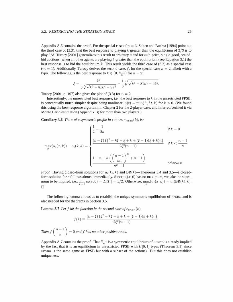
In this chapter we consider the natural n-player generalization of the 2-player game defined byEquation 2.4. We now include the following theorem from the auction theory literature2 givingthe unique symmetric Nash equilibrium of FPSB. This serves as the gold standard for all of ourapproximation techniques.
Theorem 3.1 (McAfee and McMillan, 1987, p. 709) The unique symmetric Nash equilibrium forFPSB with n players having types i.i.d. with cdf F , and a lowest possible type A is
a(t) = t−
∫ t
A
F (x)n−1 dx
F (t)n−1.
For U [A,B] types this isA+ n− 1
n· t, and for U [0, 1]:3
n− 1n· t.
3.1 Measuring Solution Quality: The ε Metric
Since our techniques are based on approximations to underlying games of interest, we need a wayto assess solution quality. There are three broad sources of inaccuracy for our solutions: (1) weconsider restricted strategy spaces and could miss better strategies (even if they are in the restrictedspace since we may incompletely explore it), (2) our simulation-based payoff estimates can beriddled with sampling error (especially when the simulations take minutes per game), and (3) weintroduce other approximations, such as reducing the number of players (Section 3.5). For thesereasons, the equilibria we derive will often not correspond to equilibria in the underlying game.In light of this, we need a measure of the quality of the strategies we find when they are not inequilibrium.
Suppose that, using some approximation Γ to a game Γ, we find an equilibrium profile s∗ ofΓ. We want to determine how closely s∗ approximates an equilibrium in Γ. If we could find anequilibrium s∗ of Γ we could compare s∗ and s∗ directly. Of course, if we could do that then therewas no need to approximate Γ in the first place. Also, the comparison between s∗ and s∗ is notnecessarily meaningful if there is more than one equilibrium in Γ.
A more natural way to answer the question is to measure the potential gain to deviating froms∗ in Γ. Ideally the answer is zero and s∗ is an equilibrium for Γ as well as Γ. In that case, Γis a perfect substitute for Γ for the purpose of finding an equilibrium profile. More generally, thesmaller the gain from deviating from s∗ in Γ, the more faithful an approximation is Γ. To this end,we define the ε of a profile, following Turocy’s [2001] usage.
Definition 3.2 (Epsilon of a Profile) For a symmetric game Γ = 〈n, S, u()〉 and strategy profiles (typically an equilibrium in some approximation of Γ), we denote by εΓ(s) the potential gain to
2Krishna [2002] provides a textbook treatment.3Kagel and Levin [1993] generalize the result for the U [0, 1] case to mth-price, single-good, sealed-bid auctions:
n− 1
n + 1−m· t, (3.1)
yielding the familiar truthful bidding result for the first and second price case [Vickrey, 1961].

3.2. RESTRICTING THE STRATEGY SPACE 23
deviating from s in Γ:
εΓ(s) ≡ maxs′∈S
u(s′, s)− u(s, s).
Alternatively, we can express ε as a percentage:
ε%Γ(s) ≡ εΓ(s)u(s, s)
· 100.
This definition follows the standard notion of approximate equilibrium. Profile s is an εΓ(s)-Nash equilibrium of Γ, and εΓ(s) = 0 if and only if s is a Nash (i.e., a 0-Nash) equilibrium of Γ.Henceforth, we drop the game subscript when understood in context.
A propitious feature of the ε metric is that εΓ(s) can be evaluated even when we know only avanishing fraction of the payoff function of Γ. In particular, we only need to know the payoffs for theunilateral deviations from s. In a symmetric n-player game with S strategies, this means evaluatingfewer than nS cells of the payoff matrix out of
(n+S−1
n
), or Sn in the case of a nonsymmetric game.
3.2 Restricting the Strategy Space
A strategy is a mapping from an agent’s private information (type), and the information revealedduring the game, to an action. In the one-shot games considered in Chapter 2 there is no infor-mation revelation (by definition of a one-shot game) and the private information and actions areone-dimensional (real numbers). So strategies in that context are one-dimensional functions fromtype to action.
The first step in our methodology for empirically analyzing games is to restrict the game byconstructing a finite set of candidate strategies. In FPSB, the strategy space is the set of functionsfrom the reals to the reals (type to action). One restriction of this strategy space is to consideronly strategies of the form a(t) = kt for specific values of k.4 This is a natural parameterizationfor FPSB, generalizing truthful bidding (a(t) = t) with a bid shading factor, k. To restrict thestrategy space less severely, we could add a translational parameter b to allow affine linear strategies(kt + b). In fact, by introducing 3K − 1 parameters, we can allow piecewise linear strategies ofup to K pieces per Equation 2.2. For one-shot games with one-dimensional types (e.g., the gamesin Chapter 2 and their generalizations to more than two players) such piecewise linear strategyparameterizations will tend to suffice. Such parameterizations are appealing because they entail nodomain knowledge—the parameters can be chosen automatically. For more complicated games, thestrategy space will be too large to parameterize so naively and we rely on the manual construction ofa strategy parameterization. This may be done by starting with a baseline strategy and generalizingit via parameters. The baseline strategy may be utterly simplistic, naive, and perform miserably.But as long as the space of strategies allowed by the parameterization includes smarter strategies(and they need not be identifiable as such a priori) then our methodology has hope of finding them.For FPSB, the baseline strategy of truthful bidding is as bad as not participating, guaranteeing zeroutility. But introducing a simple shading parameter (without knowing a good setting for it) allowsour methodology to approximate the unique symmetric Nash equilibrium of the underlying game.5
The next section shows how.
4Selten and Buchta [1994] dub this ray bidding.5There are other asymmetric equilibria [Milgrom and Weber, 1985].

24 CHAPTER 3. EMPIRICAL GAME METHODOLOGY
In Chapter 4 we apply this method of generating candidate strategies to the Simultaneous As-cending Auctions domain, and in Chapter 6 we apply it to the Trading Agent Competition travel-shopping domain. Following is the definition of the restricted form of FPSB that we use throughoutthis chapter.
Definition 3.3 (FPSBn) In the n-player first-price sealed-bid auction, player i has a private valueti, decides to bid ai, and obtains payoff ti − ai if its bid is highest and zero otherwise.6 FPSBnis the special case where ti are i.i.d. U [0, 1], and agents are restricted to parameterized strategies,bidding ai(ti) = kiti for ki ∈ [0, 1], for all i ∈ {1, . . . , n}. We denote strategies in FPSBn by theparameter k.
We now establish theoretical results to which we can compare the empirical methods in the restof this chapter.
Theorem 3.4 The expected payoff for an agent playing ki against everyone else playing k in FPSBnis:
ui(ki, k) =
⎧⎪⎪⎪⎪⎪⎪⎪⎪⎪⎪⎨⎪⎪⎪⎪⎪⎪⎪⎪⎪⎪⎩
12n
if ki = k = 0
1− ki
n+ 1
(ki
k
)n−1
if ki ≤ k
(1− ki)((n− 1)k2i − (n− 1)k2)
2(n+ 1)k2i
otherwise.
Appendix A.5 contains the proof.
Theorem 3.5 The best response to everyone else playing k in FPSBn is:
BR(k) ≡ arg maxki
ui(ki, k) =
⎧⎪⎪⎪⎪⎪⎪⎪⎪⎨⎪⎪⎪⎪⎪⎪⎪⎪⎩
undefined if k = 0
ξ if k <n− 1n
n− 1n
if k ≥ n− 1n
,
(3.3)
where ξ ≡3√
3(k2(n2 − 1
) (9n+
√3(n+ 1) ((n− 1)k2 + 27(n+ 1)) + 9
))2/3
− 32/3k2(n2 − 1
)3(n+ 1) 3
√k2(n− 1)
(9n2 + 18n+ (n+ 1)3/2
√3(n− 1)k2 + 81(n+ 1) + 9
) .
6In the case of ties (though these happen with probability zero in the infinite game with nondegenerate strategies), oneof the bidders with the highest bid is chosen with equal probability (and thus in expectation each high bidder i receives(ti − ai)/k in a k-way tie). Formally, the full payoff function is:
ui(t, a) =
8>><>>:
ti − ai
|{x ∈ a | x = max(a)}| if ai = max(a)
0 otherwise.
(3.2)
3.2. RESTRICTING THE STRATEGY SPACE 25
Appendix A.6 contains the proof. For the special case of n = 3, Selten and Buchta [1994] point outthe third case of (3.3), that the best response to playing k greater than the equilibrium of 2/3 is toplay 2/3. Turocy [2001] generalizes this result to arbitrary n and formth-price, single-good, sealed-bid auctions: when all other agents are playing k greater than the equilibrium (see Equation 3.1) thebest response is to bid the equilibrium k. This result yields the third case of (3.3) as a special case(m = 1). Additionally, Turocy derives the second case, ξ, for the special case n = 2, albeit with atypo. The following is the best response to k ∈ (0, n−1
n ) for n = 2:
ξ =k2
3 3√√
k6 + 81k4 − 9k2− 1
33√√
k6 + 81k4 − 9k2.
Turocy [2001, p. 107] also gives the plot of (3.3) for n = 2.Interestingly, the unrestricted best response, i.e., the best response to k in the unrestricted FPSB,
is conceptually much simpler despite being nonlinear: a(t) = min(n−1n t, k) for k > 0. (We found
this using the best-response algorithm in Chapter 2 for the 2-player case, and inferred/verified it viaMonte Carlo estimation (Appendix B) for more than two players.)
Corollary 3.6 The ε of a symmetric profile in FPSBn, εFPSBn(k), is:
maxx
(ui(x, k))− ui(k, k) =
⎧⎪⎪⎪⎪⎪⎪⎪⎪⎪⎪⎪⎪⎨⎪⎪⎪⎪⎪⎪⎪⎪⎪⎪⎪⎪⎩
12− 1
2nif k = 0
(k − ξ) (ξ2 − kξ + ξ + k + (ξ − 1)(ξ + k)n)
2ξ2(n+ 1)if k <
n− 1n
1− n+ k
((n− 1kn
)n
+ n− 1)
n2 − 1otherwise.
Proof. Having closed-form solutions for ui(ki, k) and BR(k)—Theorems 3.4 and 3.5—a closed-form solution for ε follows almost immediately. Since ui(x, 0) has no maximum, we take the supre-mum to be implied, i.e., lim
x→0ui(x, 0) = E[Ti] = 1/2. Otherwise, max
x(ui(x, k)) = ui(BR(k), k).
�
The following lemma allows us to establish the unique symmetric equilibrium of FPSBn and isalso needed for the theorems in Section 3.5.
Lemma 3.7 Let f be the function in the second case of εFPSBn(k),
f(k) ≡ (k − ξ) (ξ2 − kξ + ξ + k + (ξ − 1)(ξ + k)n)
2ξ2(n+ 1).
Then f
(n− 1n
)= 0 and f has no other positive roots.
Appendix A.7 contains the proof. That n−1n is a symmetric equilibrium of FPSBn is already implied
by the fact that it is an equilibrium in unrestricted FPSB with U [0, 1] types (Theorem 3.1) sinceFPSBn is the same game as FPSB but with a subset of the actions). But this does not establishuniqueness.

26 CHAPTER 3. EMPIRICAL GAME METHODOLOGY
Theorem 3.8n− 1n
is the unique symmetric equilibrium of FPSBn.
Proof. The theorem is trivially true for n = 1. Consider the n > 1 case. That n−1n is an equilibrium
follows directly from Theorem 3.5 (alternatively, from Theorem 3.1). For uniqueness it suffices toshow that for no other k is BR(k) = k. Theorem 3.5 rules out k = 0 and Lemma 3.7 establishes
that ε(k) = 0 for k ∈ (0,n− 1n
). �
3.3 Game Simulators and Brute-Force Estimationof Games
So far, we have taken a baseline strategy (truthful bidding) for FPSB and generalized it with a naturalparameterization (bid shading fraction). We solve this restricted form of FPSB in the previoussection, showing that the restriction does not change the unique symmetric equilibrium. Still, FPSBnis an infinite game so we further restrict the strategy space by discretizing the parameters. We nowshow how to approximate a normal form version of the game via simulation. The closed-formexpressions in the previous section allow us to compare with the limiting case of infinite simulationtime and continuous parameters.
The first step in estimating the empirical game is to write a game simulator.7 A game simulatoris a function that takes as input the agent types and the agent strategies and outputs payoffs. Forexample, a game simulator for FPSBn can be written as a straightforward extension to the payofffunction in Definition 3.3 as follows:8
FPSBn(t,k)i ={ti − kiti if kiti = max({k1t1, . . . , kntn})0 otherwise,
where ki is the shade parameter employed by agent i. In this case, the implementation of thesimulator is trivial and hardly warrants the name. In subsequent chapters we consider cases wherethe payoff functions involve complicated interactions between multiple auctions and the strategiesalone run to hundreds or thousands of lines of code. Nonetheless, the principle remains the same:the simulator determines agent actions by applying the strategies to the agent types (and informationdynamically revealed during the game) and from the actions determines outcomes, i.e., payoffs.
In order to exploit some of the variance reduction techniques in the next section, we additionallyrequire that the game simulator be deterministic. This is without loss of generality as we can deriveany desired randomness in the game from the dummy player, Nature, which is given the appropriatetype distribution (Section 1.1). Framed as such, symmetry is broken, but this is overcome simply bycounting Nature only as a player for the purposes of type assignments but not in the list of strategies.
The most naive, brute-force approach to empirical game estimation has the following steps:
1. For each strategy profile (distinct combination of candidate strategies), repeat for a largenumber of samples:
a) Generate random preferences for each agent according to the type distribution (which ispart of the game definition).
7This may be thought of as the first step in the mapping of a Bayesian game to a normal form game (Definition 1.1).8With the same adjustment for tie breaking as in Equation 3.2.

3.3. GAME SIMULATORS 27
Strategy Profiles
1.15
1.2
1.25
1.3
1.35
ExpectedPayoff
Figure 3.1: Payoff matrix for an SAA game with 5 players and 3 strategies. Each column corre-sponds to a strategy profile with the symmetric profile of all playing strategy 1 on the left and theprofile with all 3 on the right. The jth dot within a column represents the mean payoff for the jthstrategy in the profile. This payoff matrix is based on over 45 million games simulated for each ofthe 21 profiles, requiring weeks of cpu time. The error bars denote 95% confidence intervals. Forthis case, the unique Nash equilibrium (all playing strategy 3) is apparent by inspection.
b) If applicable, generate the other random elements of the game (i.e., Nature’s type).
c) Run the game simulator to produce sample payoffs.
2. Average the sample payoffs for each profile.
In other words, use brute-force (also called crude or plain) Monte Carlo sampling to estimate theexpected payoffs in each cell of the payoff matrix. The above procedure yields an empirical es-timate of the restricted game. Figure 3.1 shows an example of an empirical payoff matrix for anSAA game (cf. Chapter 5). Note that as the set of candidate strategies approaches the full set ofallowed strategies in the underlying game, the empirical payoff matrix approaches the full strategic(normal) form representation. Furthermore, Armantier et al. [2000, to appear] show that a Nashequilibrium in the restricted game (what they call a Constrained Strategic Equilibrium) approachesan equilibrium in the underlying game as the allowed strategy set approaches the unrestricted set.
As an example of the applicability of step 1b, suppose that coin flips are used to break ties inFPSBn. We could cast this as a game with Nature having discrete type chosen uniformly from then! permutations of {1, . . . , n}. In the case of ties, the player appearing first in Nature’s list wins.For simple games like FPSB and others in Chapter 2, we can typically keep the utility functiondeterministic by assuming that the agents split the surplus in the case of a tie, this being equivalent

28 CHAPTER 3. EMPIRICAL GAME METHODOLOGY
in expectation to deciding the winner randomly. For more complicated games such as the TradingAgent Competition (see Chapter 4), the random elements are not so easily distilled out.9
For easier applicability of the variance reduction techniques in the next section, we restrictNature’s type to be a single U [0, 1] random variable. A simple trick makes this w.l.o.g. for arbitrarytie-breaking or other random elements in a game. Namely, the mechanism includes a pseudorandomnumber generator (RNG) that is seeded with Nature’s type. Then, for example, in the case of tiesthe mechanism assigns its next pseudorandom (i.e., not random) number to each of the tying biddersin turn and then picks the one with the highest number. Including a RNG in the game simulator is amatter of adding a single equation. We propose ran0 from Numerical Recipes [Press et al., 1992]:
• Constants: a = 75, m = 231 − 1.
• Initialize r to Nature’s type times m.
• Successive random numbers: r ← a · r (mod m).
This simple RNG is considered simulation-quality as long as the 231 (∼ 2 billion) period suffices,which it will for any reasonable game—certainly all the games, including TAC, considered in thisthesis. Specifically, we require that a single instance of the game uses fewer than 231 randomnumbers. (If not, a more sophisticated RNG would be employed [Press et al., 1992].)
We test the brute-force estimation method on FPSB4 by restricting the game to 41 strategies (k ∈{0, 1/40, . . . , 1}) simulating the game 15,000 times for each of the
(4+41−1
4
)= 135, 751 strategy
profiles. Figure 3.2 shows ε(k) for every pure symmetric strategy profile—all agents playing k (i.e.,bidding k · t). This method indeed converges on the equilibrium of the underlying game, but thecomputational burden is significant, even with such a simple game as FPSB.
3.4 Variance Reduction in Monte Carlo Sampling
The core problem in game estimation is determining the payoffs in the cells of the payoff matrix—that is, estimating the expected payoffs for a fixed strategy profile given the distribution of agents’and Nature’s types. Given that we have defined a function—the game simulator—that performs sucha mapping, there are a number of off-the-shelf techniques that can be applied [Ross, 2001; Press etal., 1992; Galassi et al., 2002; L’Ecuyer, 1994]. These are known as variance reduction techniquesfor Monte Carlo estimation. They serve to improve the efficiency of the procedure presented inSection 3.3, potentially reducing by orders of magnitude the number of samples (game simulations)to estimate a payoff matrix at a given level of statistical significance.
Control Variates
The method of control variates is one such standard variance reduction technique [Ross, 2001]. Itimproves the estimate of expected payoffs by exploiting correlation of payoffs with summaries ofthe randomness in the game. The idea is to replace sampled payoffs with payoffs that have beenadjusted for “luck” such that the mean payoffs are unaffected but the variance is reduced. Forexample, in FPSB, we expect an agent’s valuation to correlate positively with its surplus. Thus,we bump up an agent’s payoff when it has a low valuation and scale it down when it has a high
9In fact, this would be quite hopeless—though possible in principle, just as in principle it is possible to represent the fullTAC game or chess in strategic form.

3.4. VARIANCE REDUCTION IN MONTE CARLO SAMPLING 29
0 0.2 0.4 0.6 0.8 1Symmetric strategy profile
0
0.05
0.1
0.15
0.2
0.25
0.3
0.35Epsilon
Figure 3.2: Evaluation of the pure symmetric (homogeneous) profiles for an empirical estimation ofFPSB4. The arrow at k = 3/4 shows the unique symmetric equilibrium for the underlying infinitegame.
valuation such that the positive and negative adjustments average out to zero or near zero. Thisstraightforwardly reduces variance in the payoffs. By sampling these adjusted payoffs it will tendto take fewer samples to converge to a good approximation of the true expected payoffs.
Consider a game Γ defined by a game simulator Γ(t, s) mapping types (agents plus Nature)and strategy profiles to payoffs. In general, we seek a function g from types to payoff estimates.For every strategy profile s, we then use g to adjust each sampled payoff Γ(t, s) by subtractingg(t)−Et[g(t)]. If the game simulator itself were used as g, i.e., g(t) ≡ Γ(t, s), then every sampledpayoff would get replaced by the true expected payoff. Of course, if we knew the expectation ofthe game simulator we would not need Monte Carlo approaches in the first place. So the trick is tofind a g for which we can derive E[g(t)], or at least estimate it more easily and accurately than wecan E[Γ(t, s)]. Theorem 3.4 provides a closed-form expression for E[FPSBn(t, s)] for symmetricprofiles s and unilateral deviations from symmetric profiles. So for FPSBn we really do know theexpectation of the game simulator. That gives us the full empirical payoff matrix to infinite precisionand for arbitrarily fine discretization of the strategy space.
Even for such a simple game as FPSBn, a closed-form solution for expected payoff was nottrivial to find. Next best, suppose we could determine analytically how expected payoff varies witha single agent’s type. In FPSB2 the expected payoff for an agent with specific type t playing kagainst an opponent with type T ∼ U [0, 1] playing k′ is (t − kt)Pr(kt > k′T ) = (1 − k)kt2/k′.(Note the difference from Theorem 3.4 in that we now consider expected payoff for a specific typerather than finding the expectation over own type.) Letting
g(t) =(1− k)kt2
k′,

30 CHAPTER 3. EMPIRICAL GAME METHODOLOGY
we integrate to find
E[g(t)] =(1− k)k
3k′.
This derivation generalizes straightforwardly to n players (from the perspective of player i):
g(ti) =(1− ki)kn−1
i tni∏j �=i
kj
, (3.4)
E[g(ti)] =(1− ki)kn−1
i
(n+ 1)∏j �=i
kj
. (3.5)
(There are 3 special cases: (1) g(ti) = 0 if ki = 0 and for some j = i, kj > 0, (2) g(ti) = 12n if
ki = 0 ∀i ∈ {1, . . . , n}, (3) otherwise, with z players playing k = 0, ignore them and substituten← n− z above.)
For more complex games (such as those addressed in subsequent chapters), we would not typ-ically be able to derive any estimator g analytically. Instead we can estimate it with an initial runof brute-force Monte Carlo samples and fit a function to the data. This is more likely to be feasi-ble if g does not depend on the strategy profile so that we do not need to generate a distinct dataset (pairings of types and payoffs) for every profile. Of course, payoff does depend on the strate-gies, but since g needs only to estimate the payoffs we can typically find a function from typesalone that correlates with payoff. To avoid introducing bias in the adjusted payoffs we use a dis-tinct set of samples to estimate g, but even if we use the same set of samples the bias goes to zeroas the number of samples increases [L’Ecuyer, 1994]. Returning to FPSB, we might generate adata set pairing a single agent’s type with payoff across all or a random subset of profiles and per-form simple linear regression to find g(t) = βt + α. This means that a payoff x is adjusted tox− (g(t)−E[g(t)]) = x− βt− α+ βE[t] + α = x− β(t−E[t]). In general, any constant termin g cancels out and so from now on we ignore them. In particular, we use g(t) = βt instead ofβt+ α.
Preliminary experiments with FPSB4 (and strategy granularity of 1/20) support the hypothesisthat the better g approximates the true expected payoff function, the greater the variance reduction.For example, for the equilibrium profile (k = 3/4), linear regression (the control variate methodrequiring no domain knowledge, analytic results, or extensive simulation) achieved a 41% reductionin variance. Linear regression on samples exclusively from the equilibrium profile happened to yielda similar enough control variate that it achieved negligible additional variance reduction. The linearmodels achieve most of the gain possible even by the analytically determined control variate ofEquations 3.4 and 3.5 which achieves a 56% reduction in variance. Figure 3.3 plots the controlvariates:
1. g(t) = 0, i.e., no control variate adjustment.
2. g(t) = 0.17t− 0.03, determined by linear regression indiscriminate of profile.
3. g(t) = 0.20t − 0.05, determined by linear regression for samples exclusively from the equi-librium profile (all playing k = 3/4).
4. g(t) = t4/4, which is Equation 3.4 with n = 4 and k = 〈34 , 34 ,
34 ,
34 〉.

3.4. VARIANCE REDUCTION IN MONTE CARLO SAMPLING 31
0 0.2 0.4 0.6 0.8 1t
-0.05
0
0.05
0.1
0.15
0.2
0.25g
�t
�
1
2
3
4
Figure 3.3: Four control variates, g(t), for FPSB4.
And Figure 3.4 shows the variances of adjusted payoff for the above control variates along with (asa sanity check)
5. g(t) = FPSB4(t, 〈34 , 34 ,
34 ,
34 〉), for which Theorem 3.4 gives E[g(t)].
In general, with multidimensional types, including Nature’s, it may not be obvious how theserandom elements influence payoffs. The dimensionality does not have to be very high before it be-comes very hard to empirically determine meaningful relationships between types and payoffs. Forexample, imagine a game involving bidding for many goods with an agent’s type being the vectorof valuations for each. Depending on the specifics of the game we might expect the sum or the maxof an agent’s valuations to correlate with payoff. It would take a sophisticated learning algorithmwith a lot of data (i.e., many game simulations) to rival a simple linear regression from sum or maxvaluation to payoff. Thus, when we have sufficient domain knowledge—such as knowing that thesum or the max are good summary statistics—we introduce control variates manually. In Chapter 6we apply the method of control variates to the Trading Agent Competition game.
Other Methods: Quasi-Random and Importance Sampling
Additional variance reduction methods that we describe here but do not currently employ in any ex-periments are quasi-random sampling and importance sampling [L’Ecuyer, 1994]. For the followingvariance reduction methods, we assume that the type space is a vector of U [0, 1] random variables.This is without loss of generality since for any random variable X with cdf F , the distribution ofF−1(Y ) where Y ∼ U [0, 1] is identical to that of X [Rice, 1995].10 We then simply fold F−1 into
10Assuming that there is an interval I (not necessarily finite) such that F is zero to the left of I , one to the right, andstrictly increasing on I .

32 CHAPTER 3. EMPIRICAL GAME METHODOLOGY
1 2 3 4 5Control Variates
0
0.002
0.004
0.006
0.008
Variance
1 2 3 4 5
Figure 3.4: Empirically determined variances for five control variates for the equilibrium profile,k = 〈 34 , 3
4 ,34 ,
34 〉, in FPSB4 with strategies k ∈ {0, 1
20 , . . . , 1}. Methods 1 and 2 do not requireanalytic results nor prohibitive sampling. Method 3 requires no analytic results but requires manysamples at every profile to which it is applied. Method 4 requires analytic results that are onlyattainable for simple games. When Method 5 is feasible, no simulation is needed at all.
the definition of the game simulator. After this transformation, the domain of the game simulatoris an n-dimensional unit hypercube of U [0, 1] random variables and thus finding the expectation isequivalent to finding the n-tuple integral of the game simulator.
Quasi-random sampling means sampling the types along a uniform hypergrid rather than ac-cording to the uniform distributions. Grid sampling requires an upfront decision on granularity;however, quasi-random sequences such as Sobel sequences avoid this by generating iteratively finergrids, each iteration filling in the gaps from the previous iteration. The benefit (and the source ofthe variance reduction) is that quasi-random sequences fill a Euclidean space more uniformly thanuncorrelated random points [Press et al., 1992].
Importance sampling means sampling according to a carefully constructed alternate distributionand then applying an adjustment to return to the original distribution. The principle is that theexpectation of a random variable P with pdf p is equal to the expectation of Xp(X)/f(X) whereX is any other random variable—in particular the carefully constructed one—with pdf f . Thealternate distribution is constructed to concentrate sampling effort in regions of the domain of thefunction where more samples improve the expected-value estimate most quickly. This is estimatedusing initial brute-force Monte Carlo sampling.
3.5 Reducing the Number of Players
In Section 3.2 we reduce the strategy space to tame the complexity of very large games. Here wepresent a related technique: reducing the number of players. The idea is that although a strategy’s

3.5. REDUCING THE NUMBER OF PLAYERS 33
payoff depends on the play of other agents (otherwise we are not in a game situation at all), itmay be relatively insensitive to the exact numbers of other agents playing particular strategies. Forexample, let (s, k; s′) denote a profile where k other agents play strategy s, and the rest play s′.In many natural games, the payoff for playing any particular strategy against this profile will varysmoothly with k, with only incremental differences between contexts (s, k − 1; s′), (s, k; s′), and(s, k + 1; s′). If such is the case, we sacrifice relatively little fidelity by restricting attention tosubsets of profiles, for instance those with only even numbers of any particular strategy. To do soessentially transforms the n-player game to an n/2-player game over the same strategy set, wherethe payoffs to a profile in the reduced game are simply those from the original game where eachstrategy in the reduced profile is played twice.
The potential savings from analyzing reduced games are considerable, as they contain combi-natorially fewer profiles. In Chapter 6 we apply hierarchical player reduction to the TAC travel-shopping domain where it makes all the difference in being able to analyze the game. In thefollowing sections, we define player reduction formally and present evidence of the viability ofapproximating games by reduced versions.
Player Reduction Definition and Hierarchical Reduction
We develop the concept of player reduction in the framework of symmetric normal-form games11
(Definition 1.2) and define a reduced game as follows.
Definition 3.9 (Player-Reduced Game) Let Γ = 〈n, S, u()〉 be an n-player symmetric game, withn = pq for integers p and q. The p-player reduced version of Γ, written Γ↓p, is given by 〈p, S, u()〉,where
ui(s1, . . . , sp) = uq·i(s1, . . .︸ ︷︷ ︸q
, s2, . . .︸ ︷︷ ︸q
, . . . , sp, . . .︸ ︷︷ ︸q
).
In other words, the payoff function in the reduced game is obtained by playing the specified profilein the original q times.
The idea of a reduced game is to coarsen the profile space by restricting the degrees of strategicfreedom. Although the original set of strategies remains available, the number of agents playing anystrategy must be a multiple of q. Every profile in the reduced game is one in the original game, ofcourse, and any profile in the original game can be reached from a profile contained in the reducedgame by changing at most p(q − 1) agent strategies.
We can apply player reduction iteratively and get a hierarchy of reduced games. We note that thegame resulting from a series of reductions is independent of the reduction ordering. Let q = r · r′.Then
(Γ↓p·r)↓p= (Γ↓p·r′)↓p= Γ↓p .Consider FPSBn with n = pq. In the reduced game FPSBn↓p, each agent i = 1, . . . , p selects a
single action ki, which then gets applied to q valuations vi1 , . . . , viqto define q bids. The auction
proceeds as normal, and agent i’s payoff is defined as the average payoff associated with its qbids. Note that the game FPSBn↓p is quite a different game from either FPSBn or FPSBp. Whenrepresented explicitly over a discrete set of actions, FPSBn↓p is the same size as FPSBp, and bothare exponentially smaller than FPSBn.
11Although the methods may generalize to some degree to partially symmetric games, or to allow partial reductions ingames given in extensive form, we do not pursue such extensions here.
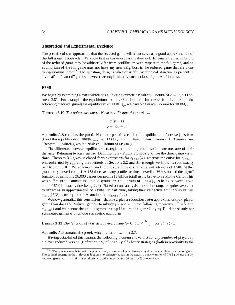
34 CHAPTER 3. EMPIRICAL GAME METHODOLOGY
Theoretical and Experimental Evidence
The premise of our approach is that the reduced game will often serve as a good approximation ofthe full game it abstracts. We know that in the worst case it does not. In general, an equilibriumof the reduced game may be arbitrarily far from equilibrium with respect to the full game, and anequilibrium of the full game may not have any near neighbors in the reduced game that are closeto equilibrium there.12 The question, then, is whether useful hierarchical structure is present in“typical” or “natural” games, however we might identify such a class of games of interest.
FPSB
We begin by examining FPSBn which has a unique symmetric Nash equilibrium of k = n−1n (The-
orem 3.8). For example, the equilibrium for FPSB2 is 1/2, and for FPSB4 it is 3/4. From thefollowing theorem, giving the equilibrium of FPSBn↓p, we have 2/3 in equilibrium for FPSB4↓2.
Theorem 3.10 The unique symmetric Nash equilibrium of FPSBn↓p is
n(p− 1)p+ n(p− 1)
.
Appendix A.8 contains the proof. Note the special cases that the equilibrium of FPSBn↓1 is k =0 and the equilibrium of FPSBn ↓n, i.e. FPSBn, is k = n−1
n . (Thus Theorem 3.10 generalizesTheorem 3.8 which gives the Nash equilibrium of FPSBn.)
The difference between equilibrium strategies of FPSB4↓2 and FPSB4 is one measure of theirdistance. Returning to our ε metric (Definition 3.2), Figure 3.5 plots ε(k) for the three game varia-tions. Theorem 3.6 gives us closed-form expressions for εFPSBn(k), whereas the curve for εFPSB4↓2
was estimated by applying the methods of Sections 3.2 and 3.3 (though we know its root exactlyby Theorem 3.10). We generated candidate strategies by discretizing k at intervals of 1/40. At thisgranularity, FPSB4 comprises 158 times as many profiles as does FPSB4↓2. We estimated the payofffunction by sampling 36,000 games per profile (5 billion total) using brute-force Monte Carlo. Thiswas sufficient to estimate the unique symmetric equilibrium of FPSB4↓2 as being between 0.625and 0.675 (the exact value being 2/3). Based on our analysis, FPSB4↓2 compares quite favorablyto FPSB2 as an approximation of FPSB4. In particular, taking their respective equilibrium values,εFPSB4(2/3) is nearly ten times smaller than εFPSB4(1/2).
We now generalize this conclusion—that the 2-player reduction better approximates the 4-playergame than does the 2-player game—to arbitrary n and p. In the following theorems, ε() refers toεFPSBn() and we denote the unique symmetric equilibrium of a game Γ by eq(Γ), defined only forsymmetric games with unique symmetric equilibria.
Lemma 3.11 The function ε(k) is strictly decreasing for 0 < k ≤ n− 1n
for all n > 1.
Appendix A.9 contains the proof, which relies on Lemma 3.7.Having established this lemma, the following theorem shows that for any number of players n,
a player-reduced version (Definition 3.9) of FPSBn yields better strategies (both in proximity to the
12FPSBn↓1 is an example (albeit a degenerate one) of a reduced game having very different equilibria than the full game.The optimal strategy in the 1-player reduction is to bid zero (as it is in the actual 1-player version of FPSB) whereas in then-player game, for n > 1, it is in equilibrium to bid a large fraction (at least 1/2) of one’s type.

3.5. REDUCING THE NUMBER OF PLAYERS 35
0.2 0.3 0.4 0.5 0.6 0.7 0.8 0.9Symmetric strategy profile
0
0.01
0.02
0.03
0.04
0.05Epsilon
Figure 3.5: Epsilons for symmetric profiles of FPSB2 (left dashed line), FPSB4↓2 (dots), and FPSB4(right dashed line). Unique symmetric equilibria (1/2, 2/3, 3/4) are indicated by arrows on thex-axis.
true equilibrium and in terms of lower ε) than does the version of the game with the number ofplayers reduced outright.13
Theorem 3.12 For all integers n and p with n > p ≥ 1,
eq(FPSBp) < eq(FPSBn↓p) < eq(FPSBn) (3.6)
and0 = ε(eq(FPSBn)) < ε(eq(FPSBn↓p)) < ε(eq(FPSBp)). (3.7)
Appendix A.10 contains the proof of (3.6), with (3.7) being an immediate consequence of (3.6) andLemma 3.11. Additionally, we show that for all FPSBn, less drastic reductions are better approxi-mations than more drastic reductions.
Theorem 3.13 For all integers n, p, and q with n > p > q ≥ 1:
eq(FPSBn↓q) < eq(FPSBn↓p) < eq(FPSBn) (3.8)
and0 = ε(eq(FPSBn)) < ε(eq(FPSBn↓p)) < ε(eq(FPSBn↓q)). (3.9)
13As suggested by Scott Page, we can sometimes do even better by first increasing the number of players before applyingplayer reduction. This works for some instances of FPSB but it would be hard to justify application of this trick in games forwhich we don’t have a gold standard (the equilibrium of the full game) to compare to.

36 CHAPTER 3. EMPIRICAL GAME METHODOLOGY
Appendix A.11 contains the proof for the first inequality of (3.8). As in Theorem 3.12, (3.9) followsdirectly from (3.8) and Lemma 3.11. The second inequality of (3.8) and the first inequality of (3.9)are given by Theorem 3.12.
Local-Effect Games
The preceding analysis is reassuring, but of course we do not actually need to approximate FPSBn,since its general solution is known. To further evaluate the quality of reduced-game approximations,we turn to other natural games of potential interest. Facilitating such studies was precisely themotivation of the authors of GAMUT [Nudelman et al., 2004], a flexible software tool for generatingrandom games from a wide variety of well-defined game classes. Using GAMUT, we can obtainrandom instances of some class, and examine the relation of the original games to versions reducedto varying degrees. The advantage of a generator such as GAMUT is that we can obtain a full gamespecification quickly (unlike for TAC), of specified size based on our computational capacity foranalysis. Moreover, we can sample many instances within a class, and develop a statistical profileof the properties of interest.
Here we focus on a particular class known as local-effect games (LEGs) [Leyton-Brown andTennenholtz, 2003], a localized version of congestion games motivated by problems in AI andcomputer networks. Specifically, we consider symmetric bi-directional local-effect games randomlygenerated by GAMUT by creating random graph structures and random polynomial payoff functionsdecreasing in the number of action-nodes chosen.
In a preliminary experiment, we generated 15 symmetric LEG instances with six players andtwo strategies, and payoffs normalized on [0, 1]. For each of these we generated the corresponding3-player reduction. We then fed all 30 of these instances to GAMBIT [McKelvey et al., 1992,and see Section 2.1] which computed the complete set of Nash equilibria for each. In 11 of theoriginal games, all equilibria are pure, and in these cases the equilibria of the reduced games matchexactly. In the remaining four games, GAMBIT identified strictly mixed equilibria in both the fulland reduced games. In two of these cases, for every equilibrium in the full game there exists anequilibrium of the reduced game with strategy probabilities within 0.1. In the remaining two games,there are long lists of equilibria in the full game and shorter lists in the corresponding reduced games.In these cases, most but not all of the equilibria in the reduced game are approximations to equilibriain the full game.
In broader circumstances, we should not expect to see (nor primarily be concerned with) directcorrespondence of equilibria in the original and reduced games. Thus, we evaluate the approxima-tion of a reduced game in terms of the average ε in the original game over all its equilibrium profilesin the reduced game. Note that to calculate this measure we need not be able to solve the full game.Since the games under consideration are symmetric, our assessment includes only the symmetricequilibria, where every agent plays the same (mixed) strategy.14
We evaluated this metric for 2-strategy local-effect games with n players, for n ∈ {4, 6, 8, 10, 12}.Figure 3.6 shows the result of generating between 200 and 10,000 games in each of the n-playergame classes and computing the ε metric for every possible reduction of every game, starting withthe most drastic reduction—to one player—and ending with the highest-fidelity reduction, i.e., tohalf as many players. We also include the average ε for the social optimum (the profile maximizingaggregate payoff) in each game class as calibration. We find that the social optimum fares better
14Symmetric games necessarily have symmetric equilibria—see Appendix C—though they may have asymmetric equi-libria as well.
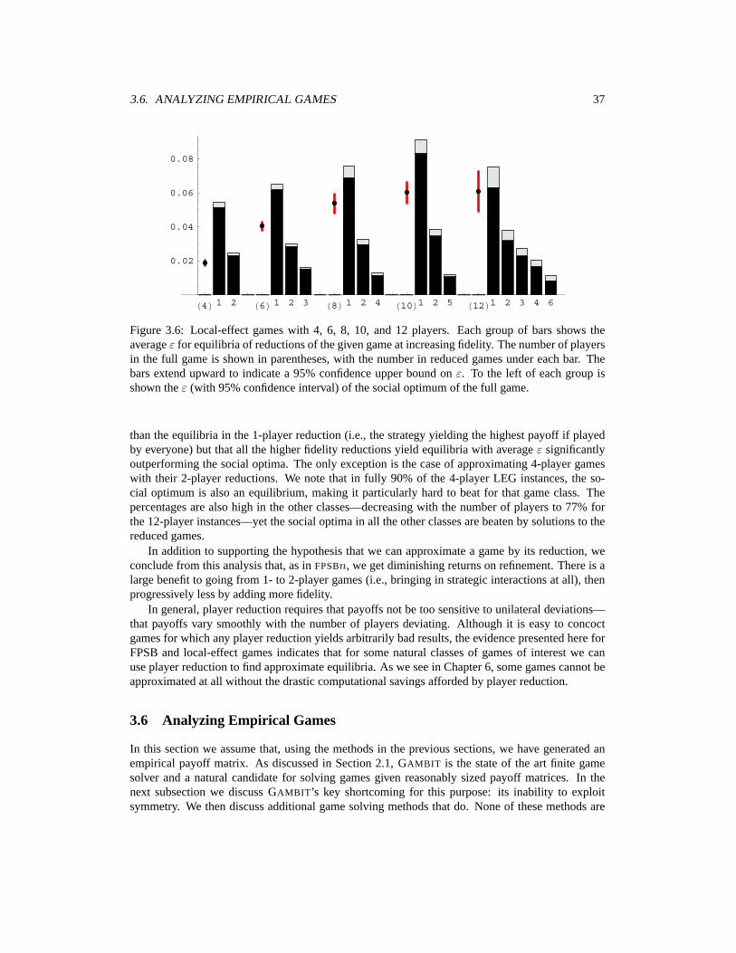
3.6. ANALYZING EMPIRICAL GAMES 37
�4� 1 2 �6� 1 2 3 �8� 1 2 4 �10�1 2 5 �12�1 2 3 4 6
0.02
0.04
0.06
0.08
Figure 3.6: Local-effect games with 4, 6, 8, 10, and 12 players. Each group of bars shows theaverage ε for equilibria of reductions of the given game at increasing fidelity. The number of playersin the full game is shown in parentheses, with the number in reduced games under each bar. Thebars extend upward to indicate a 95% confidence upper bound on ε. To the left of each group isshown the ε (with 95% confidence interval) of the social optimum of the full game.
than the equilibria in the 1-player reduction (i.e., the strategy yielding the highest payoff if playedby everyone) but that all the higher fidelity reductions yield equilibria with average ε significantlyoutperforming the social optima. The only exception is the case of approximating 4-player gameswith their 2-player reductions. We note that in fully 90% of the 4-player LEG instances, the so-cial optimum is also an equilibrium, making it particularly hard to beat for that game class. Thepercentages are also high in the other classes—decreasing with the number of players to 77% forthe 12-player instances—yet the social optima in all the other classes are beaten by solutions to thereduced games.
In addition to supporting the hypothesis that we can approximate a game by its reduction, weconclude from this analysis that, as in FPSBn, we get diminishing returns on refinement. There is alarge benefit to going from 1- to 2-player games (i.e., bringing in strategic interactions at all), thenprogressively less by adding more fidelity.
In general, player reduction requires that payoffs not be too sensitive to unilateral deviations—that payoffs vary smoothly with the number of players deviating. Although it is easy to concoctgames for which any player reduction yields arbitrarily bad results, the evidence presented here forFPSB and local-effect games indicates that for some natural classes of games of interest we canuse player reduction to find approximate equilibria. As we see in Chapter 6, some games cannot beapproximated at all without the drastic computational savings afforded by player reduction.
3.6 Analyzing Empirical Games
In this section we assume that, using the methods in the previous sections, we have generated anempirical payoff matrix. As discussed in Section 2.1, GAMBIT is the state of the art finite gamesolver and a natural candidate for solving games given reasonably sized payoff matrices. In thenext subsection we discuss GAMBIT’s key shortcoming for this purpose: its inability to exploitsymmetry. We then discuss additional game solving methods that do. None of these methods are

38 CHAPTER 3. EMPIRICAL GAME METHODOLOGY
original; however, to our knowledge we are the first to apply replicator dynamics (Section 3.6) as asolution method for large games [Wellman et al., 2003c].
Existing Game Solvers and Symmetry
GAMBIT proceeds by iteratively eliminating strongly dominated strategies and then can apply amyriad of algorithms for solving the game, most notably the simplicial subdivision algorithm [McK-elvey and McLennan, 1996] to enumerate the complete set of Nash equilibria. GAMBIT also hasalgorithms for solving extensive form games but we do not employ them in this thesis.
The problem with using GAMBIT in its current implementation is that it cannot take advantageof symmetry in a game. As noted in Section 1.2, a symmetric n-player game with S strategies has(n+S−1
n
)different profiles. Without exploiting symmetry, the payoff matrix requires Sn cells (each
with n payoffs). This entails a huge computational cost just to store the payoff matrix. For example,for a 5-player game with 21 strategies, the payoff matrix needs over four million cells comparedwith 53 thousand when symmetry is exploited. Even for n and S in single digits, this differencequickly chokes GAMBIT on games that methods exploiting symmetry have no trouble with. Forexample, in many experiments we have run on 5-player, 5-strategy games, GAMBIT took hours orsometimes days to find all the Nash equilibria when it could find them at all. Asking GAMBIT tofind only a sample equilibrium can be much faster. Still, there are games that GAMBIT fails to evenload into memory that methods that do exploit symmetry can solve.
Two methods for searching for Nash equilibria that are readily extended to exploit symmetry arefunction minimization and replicator dynamics. We employ both of these methods in subsequentchapters to find sample equilibria.
Solving Games by Function Minimization
By Definition 3.2, ε()—a function from mixed strategy profiles to the reals—equals zero at s if andonly if profile s is a Nash equilibrium. Since ε() is bounded below by zero, we can apply functionminimization techniques to solve games: the global minimum of ε() corresponds to a Nash equilib-rium. The problem with minimizing ε() however is that it is neither continuous nor differentiable.The following function is continuously differentiable, and still retains the key properties of ε()—bounded below by zero and equal to zero only at Nash equilibria15—that allow us to find equilibriaby globally minimizing it [McKelvey and McLennan, 1996].
f(s) =∑s′∈S
max[0, u(s′, s)− u(s, s)]2,
Following Walsh et al. [2002], we modify f() (compared to ε()) in that its domain is the set ofmixed strategies rather than mixed strategy profiles. In other words, we are limiting the search tosymmetric equilibria (see Appendix C), which vastly speeds it up. We can search for the root of fusing the Amoeba algorithm [Press et al., 1992], a procedure for nonlinear function minimizationbased on the Nelder-Mead method [Nelder and Mead, 1965]. For our experiments in Chapter 5 weuse an adaptation of Amoeba developed by Walsh et al. [2002] for finding symmetric mixed-strategyequilibria in symmetric games.
15This is because f(s), like ε(s), is positive iff any pure strategy is a strictly better response than s is to itself.

3.6. ANALYZING EMPIRICAL GAMES 39
Solving Games by Replicator Dynamics
In his original exposition of the concept, Nash [1950] suggested an evolutionary interpretation of(what we now call) the Nash equilibrium. That idea can be codified as an algorithm for findingequilibria by employing the replicator dynamics formalism introduced by Taylor and Jonker [1978]and Schuster and Sigmund [1983].16 Replicator dynamics refers to a process by which a populationof strategies—where population proportions of the pure strategies correspond to mixed strategies—evolves over generations17 by iteratively adjusting strategy populations according to performancewith respect to the current mixture of strategies in the population. When this process reaches a fixedpoint, every pure strategy that has not died out is performing equally well given the current strategymixture. Weibull [1995] shows that for two-player, two-strategy games, fixed points of a broadclass of replicator processes are Nash equilibria if neither strategy is extinct. For n-player games,the set of fixed points that are locally asymptotically stable (all states sufficiently close converge tothe same state) are a subset of the set of Nash equilibria [Friedman, 1991].
Although a more general form of replicator dynamics can be applied to nonsymmetric games[Gintis, 2000], it is particularly suited to searching for symmetric equilibria in symmetric games.
To implement this approach, we choose an initial population proportion for each pure strategyand then update them in successive generations so that strategies that perform well increase in thepopulation at the expense of low-performing strategies. The proportion pg(s) of the populationplaying strategy s in generation g is given by
pg(s) ∝ pg−1(s) · (EPs −W ),
where EPs is the expected payoff for pure strategy s against n − 1 players all playing mixedstrategies according to the population proportions, and W is a lower bound on payoffs (e.g., theminimum value in the payoff matrix). To calculate the expected payoff EPs from the payoff matrix,we average the payoffs for s in the profiles consisting of s concatenated with every profile of n− 1other agent strategies, weighted by the probabilities of the other agents’ profiles. The probability ofa particular profile 〈n1, . . . , nS〉 of n agents’ strategies, where ns is the number of players playingstrategy s, is
n!n1! · · ·nS !
· p(1)n1 · · · p(S)nS . (3.10)
(This is the multinomial coefficient multiplied by the probability of a profile if order mattered.)Figure 3.7 shows an example of the replicator dynamics evolving to a particular symmetric mixedequilibrium in an SAA game (confer Chapter 5).
If the population update process reaches a fixed point, then the final population proportionsare a candidate mixed strategy equilibrium. We verify directly that the candidate is in equilibriumby checking that the ε is zero or on par with the tolerance of the replicator dynamics calculations(typically 10−10). In other words, we verify that the that the evolved strategy is a best response toitself. In all the experiments reported in this thesis, this process indeed reaches a fixed point andthese fixed points always correspond to Nash equilibria. However, we have found examples forwhich the replicator dynamics do not converge and the population proportions cycle.
16Weibull [1995] attributes the the term “replicator” to Dawkins [1976].17Instead of using discrete generations, the process can be defined continuously by a system of differential equations.

40 CHAPTER 3. EMPIRICAL GAME METHODOLOGY
0 20 40 60 80 100
0
0.1
0.2
0.3
0.4
0.5
0.6
0.7
16
17
18
1920
Figure 3.7: Replicator dynamics for an SAA game with 5 players and 5 strategies {16, . . . , 20}evolving in about 100 generations to a symmetric mixed equilibrium of all agents playing strategy16 with probability 0.754 and 17 otherwise.
3.7 Interleaving Analysis and Estimation
Since estimating cells of a payoff matrix tends to be far more compute-intensive than finding Nashequilibria of a given payoff matrix, we discuss ways to use equilibrium analysis as a guide forselective sampling of profiles.
In related work, Walsh et al. [2003] show one way to apply this idea, interleaving the MonteCarlo simulation with the Nash equilibrium computation to concentrate sampling on profiles forwhich more accurate payoff estimates will yield better estimates of the Nash equilibria of the under-lying game, allowing substantial reduction in the number of simulations needed to estimate a payoffmatrix.
Their approach is inspired by information theory in that they choose the next profile to samplebased on which has the greatest potential to change the maximum likelihood estimate for a Nashequilibrium. Note that this and other selective profile sampling techniques are complementary tothe Monte Carlo variance reduction techniques of Section 3.4 which entails intelligent sampling ofthe underlying type distribution to speed up estimation of expected payoffs for a particular profile.
We have explored a related approach using a variation of replicator dynamics in which we si-multaneously gather sample payoffs to form the estimated payoff matrix and evolve towards equilib-rium. We start with an initial set of population proportions for each pure strategy. Then, as before,we repeatedly sample from the preference distribution and simulate the game to produce samplepayoffs. However, now strategies are randomly drawn to participate according to their populationproportions. Then, after a relatively small number of samples—long before we have confidencethat they are good estimates of the expected payoffs—we apply the replicator dynamics using the

3.8. SENSITIVITY ANALYSIS 41
realized average payoffs.18 Then, given the new population proportions, we iterate, calculating asequence of new generations, except that for each generation we retain the accumulated estimate ofaverage payoffs from previous generations, and aggregate the old and new sample information. Theiteration of generations continues until the population proportions are stationary with respect to thereplicator dynamics.
The above procedure straightforwardly accumulates a statistically precise estimate of the ex-pected payoff matrix. However, the sampling is biased: strategies that are more successful (andthus more highly represented in the population) are sampled more often. We conjecture that thisapproach can be more efficient than uniform sampling, especially for problems with a large numberof permissible strategies. Since many of them will likely not be present in a Nash equilibrium—thatis, their population fractions will converge to zero—extensive sampling to lower the standard errorof the estimated payoff would be wasteful.
3.8 Sensitivity Analysis
Since our game analysis is based on payoff matrices estimated by repeated simulation of games, animportant question is whether the equilibria we find are robust or if they would change with furthersampling. Each expected payoff in the matrix is estimated (the maximum-likelihood estimate) bythe sample mean but we need statistical confidence bounds on our estimate. More generally, weseek a probability distribution for the true expected payoff, representing our belief.
Estimating the Expected Value of a Random Variable
Since we have no a priori information about the distribution of the payoffs, our estimates of themare based only on our sampling. By the Central Limit Theorem,19 the mean of a sample from anydistribution converges to a normal distribution as the number of samples grows. For small samplesizes (less than 30) it is considered better to use a t-distribution. A corollary of Fisher’s Theoremtells us that for samples from a normal distribution with true mean μ and sample size n with samplemean X and sample variance S2, (X − μ)/
√S2/n has a t-distribution with n − 1 degrees of
freedom. Even when the underlying distribution is not normal, using such a t-distribution tends tobe a better estimate.20 Henceforth, I will refer to the distribution of the sample mean as normaleven though we use the more faithful t-distribution for small sample sizes in our analysis. Thekey assumption, common in statistics, is that this sample mean distribution represents a reasonablebelief for the underlying true mean—in our case, the true expected payoff. Figure 3.8 shows anexample of how this assumption is reasonable even for highly non-normal distributions.
Approximating a Distribution over Payoff Matrices
Given a normal distribution for each of the expected payoffs in the payoff matrix we seek a distri-bution representing our belief of the space of possible payoff matrices. This problem is simplified
18Monte Carlo variance reduction techniques can also be applied here.19Confer any statistics textbook, e.g., Rice [1995].20 To test this common presumption, we performed our own experiment. Using a class of highly non-normal distributions
(0/1 Bernoulli trials with particular success probabilities) we repeated the following steps: (1) pick a distribution from theclass (knowing the mean μ), (2) gather n samples from it, (3) use a proper scoring rule (quadratic) to score the estimated pdfof the sample mean, using a t-distribution and a normal. The steps were repeated for many underlying distributions from theclass (with μ varying from 0 to 1) and for many different sample sizes. We conclude that a t-distribution indeed outperformsa normal distribution, until the sample size grows beyond 30 where the difference begins to vanish.

42 CHAPTER 3. EMPIRICAL GAME METHODOLOGY
0.3 0.4 0.5 0.6 0.7 0.8
50
100
150
200
250
300
Figure 3.8: Histogram of the mean of 30 samples of a starkly bimodal distribution (0/1 Bernoullitrials with success probability 1/2—i.e., the density function has all its mass concentrated on 0 and1).
by the fact that there is no covariance between payoffs in different cells. This is because they arefunctions of distinct vectors of independent random variables and thus must be independent. Butpayoffs within a cell—those corresponding to different strategies in the same profile—do covary ingeneral. For example, in FPSB, the lower an agent’s type, the less likely it is to win (the lower itsexpected payoff) with corresponding benefit to everyone else. We typically ignore this covarianceand thus overestimate the variance of individual payoffs. This means that our sensitivity analysis isconservative in recommending additional samples (erring on the side of recommending more thannecessary).
We compute the empirical payoff matrix distribution by collecting statistics from runs of thegame simulator.21 We can then aggregate samples within a profile where allowed by symmetry. Forexample, suppose we have simulated 1000 games for the profile 〈1, 1, 1, 2, 2〉 in a 5-player game.By definition of a symmetric game, the first three expected payoffs (and the last two) must be thesame. In fact, from the 1000 games we have 3000 instances of strategy 1 playing against two othersplaying 1 and two playing 2. Since samples from the same game are correlated, we cannot treatthese as 3000 distinct instances22 but we can nonetheless improve the estimates by replacing eachsample payoff for the first three players by the average of the three (and similarly for the last two).
21It suffices to maintain a running total of the number of payoffs sampled, the sum, and the sum of the squares of thepayoffs. From these summary statistics we can compute the mean and variance (and of course the sample size)—that is, thefirst and second moments.
22Though in our sensitivity analysis in Section 5.3 we did. Nonetheless, we believe the measure is still conservativeand that even without conservative sample aggregation, the results are not suspect. This is consistent with our experience inthat most often when our sensitivity analysis tells us we need more samples, they turn out not to have been necessary. Infact, sensitivity analysis has to indicate extreme sensitivity before it to turns out that with enough additional samples, theequilibria change. In other words, our informal observation is that this form of sensitivity analysis tends to report widervariances in equilibria than there are.

3.9. RELATED WORK 43
This shows that we are getting more than 1000 samples’ worth of payoffs for the 1000 games andusing 1000 as the sample size will again ensure that we only overestimate the variance of the payoffmatrix distribution.
Assessing Sensitivity
Given a distribution over payoff matrices, we can infer a distribution over functions of the payoffmatrix. One such function of interest is of course the set of Nash equilibria, or a sample equilibriumfound by a particular solution method. Another is the ε for a particular profile (such as a candidateequilibrium).
Confidence Bounds on Mixture Probabilities
If enough samples from the payoff matrix distribution all yield the same equilibrium results thenwe would conclude that our results are insensitive to sampling noise. One way to operationalizethat criterion is to repeatedly sample payoff matrices, compute one or all symmetric equilibria, andobserve the distributions for the probability mixtures. Figure 3.9 shows an example of such a sen-sitivity measure from an SAA game (confer Chapter 5). In that example we can safely concludethat an equilibrium of the underlying restricted game involves playing strategy 16 with high proba-bility, strategy 17 with low probability, and the other strategies with zero to very low probabilities.Throughout our experiments in subsequent chapters our experience has borne out the claim that thissensitivity measure is conservative. Equilibria judged robust by this measure do not tend to changewith additional samples. In fact, only when this measure indicates extreme sensitivity do we findthat additional simulation causes the equilibrium results to change.
Confidence Bounds on Epsilon
Unfortunately, we often do not have the simulation time needed to get the sample variances lowenough to be able to say anything at all about the likely ranges of mixture probabilities in equi-librium.23 So as an alternative sensitivity assessment, we turn to our ε metric and compute, for acandidate equilibrium profile s, an empirical distribution for ε(s) in the same way that we foundempirical distributions for the mixture probabilities above, by sampling many payoff matrices fromour belief distribution and for each sample Γi computing εΓi
(s). If a fraction p of the probabilitymass is at zero then we can conclude with confidence p that we have found an actual equilibriumof the underlying restricted game. In the best case, p is near one and the conclusion is definitive. Ifnot, we can at least give probabilistic bounds on ε and make concrete the claim that s approximatesan equilibrium to the underlying (restricted) game. Figure 3.10 shows an empirical pdf (histogram)for ε of a candidate equilibrium based on an empirical estimate of a reduced TAC game (conferChapter 6).
3.9 Related Work
Several researchers have addressed game-theoretic questions in a similar empirical vein to the ap-proach presented in this chapter [Kephart et al., 1998; Armantier et al., 2000; Kephart and Green-wald, 2002; Walsh et al., 2002]. Of particular note is the Trading Agent Competition (TAC) liter-
23We find that when we can identify a pure equilibrium it tends to be far more robust (less sensitive) than when onlymixed equilibria are found.
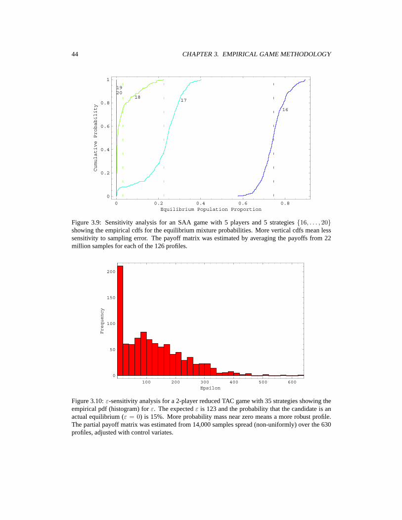
44 CHAPTER 3. EMPIRICAL GAME METHODOLOGY
0 0.2 0.4 0.6 0.8Equilibrium Population Proportion
0
0.2
0.4
0.6
0.8
1
Cumulative
Probability
16
1718
1920
Figure 3.9: Sensitivity analysis for an SAA game with 5 players and 5 strategies {16, . . . , 20}showing the empirical cdfs for the equilibrium mixture probabilities. More vertical cdfs mean lesssensitivity to sampling error. The payoff matrix was estimated by averaging the payoffs from 22million samples for each of the 126 profiles.
100 200 300 400 500 600Epsilon
0
50
100
150
200
Frequency
Figure 3.10: ε-sensitivity analysis for a 2-player reduced TAC game with 35 strategies showing theempirical pdf (histogram) for ε. The expected ε is 123 and the probability that the candidate is anactual equilibrium (ε = 0) is 15%. More probability mass near zero means a more robust profile.The partial payoff matrix was estimated from 14,000 samples spread (non-uniformly) over the 630profiles, adjusted with control variates.

3.9. RELATED WORK 45
ature which, for the case of the travel-shopping domain, we discuss in Section 6.7. There has alsobeen one study of note in the more recent supply-chain game introduced in TAC in 2003. In thisdomain, Wellman et al. [2005a] apply the basic approach of Section 3.3 along with control variates(Section 3.4) and sensitivity analysis (Section 3.8) to analyze strategic interactions in the game. Asnoted in Section 3.3, Armantier et al. [2000] define the concept of a Constrained Strategic Equi-librium (what we refer to as an equilibrium in a strategy-restricted game) and provide theoreticaljustification for an empirical game methodology. In more recent work, Armantier et al. [to appear]propose the core idea of estimating ε in the full game as a way to assess the quality of an equilib-rium in the restricted game. Additionally, they apply a similar methodology to that described here toapproximate equilibria in various auction games. As noted in Section 3.7, Walsh et al. [2003] haveaddressed the problem of reducing the computational cost of empirical payoff matrix generation. InChapter 6 we apply a similar approach but in a rather ad hoc, manual way.
Despite the common use of symmetric constructions in game-theoretic analyses, the literaturehas not extensively investigated the general properties of symmetric games. One noteworthy ex-ception is Nash’s original paper on equilibria in non-cooperative games [Nash, 1951], which (inaddition to presenting the seminal equilibrium existence result) considers a general concept of sym-metric strategy profiles and its implication for symmetry of equilibria. We include a collection ofresults about symmetric games in Appendix C. Although GAMBIT does not yet exploit symme-try in games, Bhat and Leyton-Brown [2004] present a new game-solving algorithm based on amethod by Govindan and Wilson [2003] which they extend to exploit symmetry and, especially,context-specific independencies between players’ utility functions.
Evolutionary Search for Trading Strategies
Several prior studies have employed evolutionary techniques for the analysis or derivation of tradingstrategies. An early example was an evolutionary simulation among trading agents submitted to theSanta Fe Institute (SFI) Double Auction Tournament [Rust et al., 1993].
The SFI Artificial Stock Market [Arthur et al., 1997] has been used to investigate theories oftrading behavior and market dynamics, incorporating genetic algorithms and other evolutionarymechanisms in versions of the model. This work is part of a growing literature in agent-basedfinance [LeBaron, 2000], much of which makes use of evolutionary techniques.
Price [1997] demonstrates the use of genetic algorithms (GAs) for a variety of standard indus-trial organization games (e.g., Bertrand and Cournot duopoly). In Price’s approach, the GA servesas an optimization method, employed to derive a best response. For instance, his GA model forthe duopoly games comprises populations of strategies for each producer, each updated separatelyaccording to GA rules. The search is co-evolutionary in the sense that fitness statistics are derivedby joint sampling from the pair of populations.
Cliff [1998] applied GAs to evolve improved versions of his “ZIP” trading strategy for contin-uous double auctions. Improvement in his study is defined in terms of convergence to competitiveequilibrium prices, as opposed to surplus for particular agents. The evolutionary search, therefore,is for a high-performing homogeneous trading policy, rather than a strategic equilibrium. In morerecent work, Cliff [2003] expanded the search space to include a market-mechanism dimension,thus evolving a trading strategy in conjunction with an auction rule. As above, the GA’s fitnessmeasure is in terms of aggregate market performance, rather than individual profit.
Using a co-evolutionary approach similar to that of Price discussed above, Phelps et al. [2002]employ genetic programming to derive strategies for an electricity trading game studied by Nico-laisen et al. [2001]. They then extend the model to evolve auction rules in tandem with the trading

46 CHAPTER 3. EMPIRICAL GAME METHODOLOGY
strategies. Unlike Cliff, Phelps et al. evaluate fitness of the mechanism based on aggregate perfor-mance, while evolving trading strategies based on individual performance.
Byde [2002] evaluated a parameterized range of auction mechanisms, essentially equivalent toa one-sided version of k-double auctions [Satterthwaite and Williams, 1993]. For each scenario(auction setting and distribution of private and common values), he employs the GA to evolve atrading strategy, and evaluates the average revenue of the given auction with respect to a populationof traders using that strategy.
Though sharing the same goal as this thesis (finding good trading strategies), the key differencebetween ours and the above evolutionary approaches is that we consider strategy generation gametheoretically.

Chapter 4
Price Prediction for Strategy Generation inComplex Market Mechanisms
IN WHICH we propose various approaches to price prediction as the basis for strategygeneration in interdependent auction environments.
The previous chapter presents empirical methods for generating strategic guidance in gamesthat are too complex for exact game-theoretic solutions. Here we apply the first step of thatmethodology—generating a space of candidate strategies—to two complex market games involvingbidding under uncertainty in interdependent auctions: Simultaneous Ascending Auctions (SAA)and the Trading Agent Competition (TAC) travel-shopping game. We adopt the common approachof price prediction for finding strategies in such domains.
Our approach to price prediction in TAC is based on the concept of Walrasian price equilib-rium, which we apply to SAA as well. After discussing this concept and its applicability to priceprediction in general we consider the SAA and TAC domains separately. We present a generalclass of prediction-based strategies for SAA, parameterized by particular price predictions includ-ing Walrasian equilibrium prices and self-confirming predictions. (In Chapter 5 we demonstrate therobustness of the latter strategy.) Next, we present the details of our prediction-based hotel biddingstrategy in TAC (other aspects of our TAC strategy are discussed in Chapter 6) and describe twomethods for assessing the quality of predictions. Chapter 6 discusses our game-theoretic analysis ofthe TAC game.
4.1 Interdependent Auctions: TAC and SAA
The Trading Agent Competition travel-shopping game1 pits eight travel agents against one another—each attempting to procure travel resources to put together trips for hypothetical clients. The pref-erences of these clients include preferred trip dates, premiums for better hotel rooms, and premi-ums for different types of entertainment tickets. These client preferences implicitly define a travelagent’s value function over the available goods. The agent’s task is to procure a set of goods thatachieves maximum value at minimum cost. A key feature of the TAC game is the need for agentsto participate in multiple simultaneous auctions.
1We describe the TAC game in more detail in Section 4.7. See also Wellman et al. [2003b].
47

48 CHAPTER 4. PRICE PREDICTION
This aspect of the Trading Agent Competition is characteristic of many real-world scenarios,such as bidders participating in concurrent auctions on eBay. To isolate the strategic issues involvedin simultaneously bidding for related goods, we study a simpler and more generic domain thatfocuses on a set of identical and synchronized English ascending auctions. This is the SimultaneousAscending Auctions (SAA) domain in which each agent participates concurrently in many auctions,one for each of the goods available. The auctions are independent except that no auction closes untilbidding has stopped in all of them.
Complementarity and Substitutability
Complementarity is a key feature of both SAA and TAC. Complementarity manifests when anagent’s value for a good is greater if it also obtains one or more other goods. For example, an airlinepassenger may wish to obtain two connecting segments to complete a trip. The airline, meanwhile,needs to obtain reservations for both a takeoff slot and a landing slot for each flight segment. If apair (or in general a set) of goods are each worthless without the other, they are said to be perfectcomplements. Complementarity may also be partial: my demand for ski poles drops if the costof skis becomes prohibitive, but I still may have value for one good without the other. In general,goods exhibit complementarity from the perspective of an agent when its valuation is superadditive.Given a set of goods X and valuation function,2 v : 2X → R, that assigns value to possible subsetsof X , superadditive preference means that for any Y ⊆ X , v(Y ) ≥∑
i∈Y v({i}). In other words,a bundle of goods is worth more than the sum of its parts.
When the inequality is reversed, the valuation is subadditive which implies substitutability be-tween goods. For example, alternative and contemporaneous vacation packages are perfect substi-tutes—no additional value is derived from getting both. Two cameras may be partial substitutes ifthe bulk of an agent’s value comes from getting one camera with some small additional value forhaving a second. An agent has single-unit preference iff for all Y ⊆ X , v(Y ) = maxi∈Y v({i}).In other words, goods are perfect substitutes, though not necessarily 1:1 substitutes. For the case ofsubadditive utility and especially the extreme case of single-unit preference, finding optimal strate-gies is an easier problem.
In this thesis we focus on the more difficult case of superadditive preference—complementarygoods. When an agent must bid for one resource with uncertainty about the market resolution ofcomplements, its decision presents risky tradeoffs. By predicting eventual market prices, an agentcan mitigate these risks.
4.2 Walrasian Price Equilibrium
A Walrasian price equilibrium refers to prices such that supply meets demand. It is also calleda competitive price equilibrium since it constitutes prices that would be reached in a competitiveeconomy, i.e., where all agents are price-takers.3 Even though the economies we study are notcompetitive (except in the limit as the number of agents increases) we employ Walrasian competitiveequilibria as estimates for the purposes of price prediction.
2In SAA, this value function (specified implicitly) defines an agent’s type. The same is the case for TAC: the clientpreferences induce a valuation function over all possible subsets of travel resources. To fully specify a TAC agent’s type alsorequires the initial endowment of goods. There is no such initial endowment in (our model of) SAA.
3Subject to additional assumptions, discussed below.

4.2. WALRASIAN PRICE EQUILIBRIUM 49
Consider a set of m goods4 with prices denoted by the vector p. There are n agents and eachagent’s demand for each good depends on the prices of all the goods, allowing in general for ar-bitrary complementarity and substitutability. We write xj
i (p) to denote an agent’s demand for agood, specifically, the integer number of units of good i that agent j chooses to purchase givenprices, p, for all goods (including i). When only one unit of each good is available or desired,xj
i (p) ∈ {0, 1} ∀i, j,p. The vector of agent j’s demands for all the goods is denoted xj(p). Aggre-gate demand is simply the sum of agent demands,
x(p) =∑
j
xj(p). (4.1)
Note that an agent’s valuation function defines its demand function. Specifically, an agent’s demandvector x is that which (out of all possible demand vectors) maximizes valuation minus cost (v(x)−x · p).
Prices p constitute a Walrasian equilibrium iff aggregate demand equals aggregate supply foreach good. In the case of exactly one of each of the m goods available, we have that in Walrasianequilibrium, x(p) = 1. To allow for multiple units of each good, the vector 1 is replaced withthe aggregate supply vector, y. Walras [1874] originally conceived of an iterative price adjustmentmechanism—the tatonnement protocol—for searching for equilibrium prices [Arrow and Hahn,1971]. Given a specification of aggregate demand and an initial guess p0, tatonnement iterativelycomputes a revised price vector according to:
pt+1 = pt + αt(x(pt)− y), (4.2)
where αt is a learning parameter, strictly positive, that decreases in t.5 The effect of the protocol isto nudge prices of under-demanded goods down and over-demanded goods up. If a fixed-point isreached then we have a price equilibrium.
General equilibrium theory develops technical conditions on agent preferences under whichsuch an equilibrium can be guaranteed to exist, for the case of continuous goods [Mas-Colell etal., 1995]. In our models, goods are discrete and for that case Bikhchandani and Mamer [1997]provide existence criteria. Single-unit preference is a sufficient condition for equilibrium existence,as well as other technical conditions, but for the general preference distributions we consider we arenot guaranteed existence of price equilibria.6 Indeed, there are examples in both domains of agentpreferences that admit no price equilibria. For the convergence of tatonnement to a price equilibrium(when one exists) a sufficient condition is that preferences satisfy the property of gross substitutes[Kelso and Crawford, 1982]. Unfortunately, the complementarities in both TAC and SAA patentlyviolate this property. Nonetheless, in both domains tatonnement typically converges quickly to atleast an approximate price equilibrium (i.e., prices inducing relatively small imbalances of supplyand demand).
4It is w.l.o.g. to consider m goods with exactly one unit available of each: if there are k units of one good they can beindexed and treated as distinct. Nonetheless, it is often convenient (e.g., in TAC) to allow for multiple units of each of the mgoods (i.e., m good types) and so our treatment in this section allows for that case.
5For example, in TAC (see Section 4.9), after some experimentation we set αt = 0.387 · 0.95t.6We do know that whenever a price equilibrium exists, the resulting allocations are guaranteed to be efficient [Bikhchan-
dani and Mamer, 1997].

50 CHAPTER 4. PRICE PREDICTION
4.3 The Simultaneous Ascending Auctions (SAA) Domain
The formal specification of the Simultaneous Ascending Auctions (SAA) game [Cramton, 2005]includes a number of agents, n, a number of goods, m, and a type distribution that yields valuationfunctions, vj , for the agents (plus Nature’s type, needed for tie-breaking—see Section 3.3). Eachseparate auction, one for each good, may undergo multiple rounds of bidding. The bidding issynchronized so that in each round each agent submits a bid in every auction it chooses to bid in. Atany given time, the bid price on good i is βi, defined to be the highest non-repudiable bid bi receivedthus far, or zero if there have been no bids. The bid price along with the current winner in everyauction is announced at the beginning of each new round. To be admissible, a new bid must meetthe ask price, i.e., the bid price plus a bid increment (which we take to be one w.l.o.g., allowing forscaling of the agent values): bnew
i ≥ βi + 1. If an auction receives multiple admissible bids in agiven round, it admits the highest, breaking ties randomly. An auction is quiescent when a roundpasses with no new admissible bids, i.e., the new bid prices βnew = β which become the finalprices p. When every auction is simultaneously quiescent they all close, allocating their respectivegoods per the last admitted bids. An agent’s payoff—also referred to as its surplus—is then definedby the auction outcomes, namely, the set of goods it wins, X , and the final prices, p:
σ(X,p) ≡ v(X)−∑i∈X
pi. (4.3)
Section 3.3 introduces the concept of a game simulator. As for any game, the input for theSAA simulator is the vector of agent types, t, consisting for SAA of agent valuation functions plusNature’s type, and a strategy profile s (parameterizations for SAA strategies are described below).Agent strategies plus their types determine their bid actions and so we can simulate the protocoland compute the auction outcomes. We denote the auction outcomes by Xj(t, s) for the bundle ofgoods that agent j wins and p(t, s) for the final prices, as a function of types and strategies. Thegame simulator for SAA is then:
SAA(t, s)j = σ(Xj(t, s),p(t, s)).
The Exposure Problem
Because no good is committed until all are, an agent’s bidding strategy in one auction cannot becontingent on the outcome for another. Thus, an active agent desiring a bundle of complementarygoods runs the risk that it will purchase some but not all goods in the bundle. This is known asthe exposure problem, and arises whenever agents have complementarities among goods allocatedthrough separate markets.
The exposure problem is a key motivation for designing mechanisms that take the complemen-tarities directly into account, such as combinatorial auctions [Cramton et al., 2005; de Vries andVohra, 2003], in which the auction mechanism determines optimal packages based on agent bidsover bundles. Although such mechanisms may provide an effective solution in many cases, there areoften significant barriers to their application [MacKie-Mason and Wellman, 2005]. SAA-based auc-tions are even deliberately adopted, despite awareness of strategic complications [Milgrom, 2000]—most famously the US FCC spectrum auctions starting in the mid-1990s [McAfee and McMillan,1996]. Simulation studies of scenarios based on the FCC auctions shed light on some strategicissues [Csirik et al., 2001], as have accounts of some of the strategists involved [Cramton, 1995;Weber, 1997], but the game is still too complex to admit definitive strategic recommendations.

4.4. STRAIGHTFORWARD BIDDING AND VARIATIONS 51
In general, markets for interdependent goods operating simultaneously and independently areubiquitous, and yet auction theory to date [Krishna, 2002] has little to say about how one shouldbid in simultaneous markets with complementarities. In the next sections we propose the genera-tion of candidate strategies based on price prediction and in Chapter 5 we apply the methodologyfrom Chapter 3 to find and assess good instances of these strategies, as well as demonstrate theirsuperiority over previously known strategies.
4.4 Strategies for SAA: Straightforward Bidding andVariations
If an agent knew the final prices of all m goods then its optimal strategy would be straightforward:bid on the subset of goods that maximizes its surplus at known prices. We define a class of biddingstrategies based on perceived prices in which an agent selects the subset of goods that maximizesits surplus at those prices.
First, we define an agent’s information state, B, as the t ×m history of bid prices revealed bythe auctions as of the tth round. Any strategy is then a mapping from B to a bid vector—a bid ineach of the m auctions where a zero bid is equivalent to not bidding. We denote the set of possibleinformation states by B.
Definition 4.1 (Perceived-Price Bidder) A perceived-price bidder is parameterized by a perceivedprice function ρ : B→ Z
m∗ which maps the agent’s information state, B, to a (nonnegative, integer)
perceived price vector, p. It computes the subset of goods
X∗ = arg maxX
σ(X, ρ(B))
breaking ties in favor of smaller subsets and lower-numbered goods.7 Then, given X∗, the agentbids bi = βi + 1 (the ask price) for the i ∈ X∗ that it is not already winning.
A perceived-price bidding strategy is defined by how the agent constructs p from its informationstate. In Section 4.5 we define functions, ρ, for perceived-price bidding strategies that map infor-mation state to predicted prices.
Straightforward Bidding
One example of a perceived-price bidder is the widely-studied straightforward bidding (SB) strat-egy.8 An SB agent sets p to myopically perceived prices: the bid price for goods it was winning inthe previous round and the ask price for the others:
ρi(B) = pi =
{βi if winning good i
βi + 1 otherwise,(4.4)
where β is the last (tth) row of B, i.e., the current bid prices.
7More precisely: when multiple subsets tie for the highest surplus, the agent chooses the smallest. If the smallest subset isnot unique it picks the subset whose bit-vector representation is lexicographically greatest. (The bit-vector representation ωof X ⊆ {1, . . . , m} has ωi = 1 if i ∈ X and 0 otherwise. For example, the bit-vector representation of {1, 3} ⊆ {1, 2, 3}is 〈1, 0, 1〉.)
8We adopt the terminology introduced by Milgrom [2000]. The same concept is also referred to as “myopic bestresponse”, “myopically optimal”, and “myoptimal” [Kephart et al., 1998].

52 CHAPTER 4. PRICE PREDICTION
Straightforward bidding is a reasonable strategy in some environments, such as the special caseof an SAA with no complementarities. When all agents have single-unit preference, and value everygood equally (i.e., the goods are all 1:1 perfect substitutes), the situation is equivalent to a problem inwhich all buyers have an inelastic demand for a single unit of a homogeneous commodity. For thisproblem, Peters and Severinov [2001] show that straightforward bidding is a perfect Bayes-Nashequilibrium.
If agents have additive utility, i.e., v(Y ) =∑
i∈Y v({i}), then they can treat the auctions asindependent and in this case too, SB is in equilibrium. To see this, consider the case that all otheragents are playing SB with additive preference. Then your bid in one auction does not affect yoursurplus in another. This implies the auctions can be treated independently and SB is a best response.We conjecture that SB is a Nash equilibrium in the more general subadditive case as well, but adefinitive answer to this question awaits future work.
The degenerate SAA with m = 1, i.e., a single ascending auction, is strategically equivalent toa second-price sealed-bid auction [Vickrey, 1961].9 For m > 1, however, even though additivitymakes the auctions independent, the joint strategy space allows threats such as “if you raise the priceon my good I will raise it on yours.” These will then support demand-reduction equilibria, even inthe additive case. Thus, although SB is a good strategy and is in equilibrium for at least some classesof environments without complementarities, it is not a dominant strategy in any reasonable class ofSAA games.
Up to a discretization error, the allocation in an SAA with single-unit preference is efficientwhen agents follow straightforward bidding. It can also be shown [Bertsekas, 1992; Wellman etal., 2001a] that the final prices will differ from the minimum unique equilibrium prices by at mostmin(m,n) times the bid increment. The value of the allocation, defined to be the sum of thebidder surpluses, will differ from the optimal by at most the bid increment times min(m,n)(1 +min(m,n)).
Unfortunately, none of these properties generalize to superadditive preference. The final SAAprices can differ from the minimum equilibrium price vector, and the allocation value can differfrom the optimal, by arbitrarily large amounts [Wellman et al., 2001a]. And most importantly, SBneed not be a Nash equilibrium.
v({1}) v({2}) v({1, 2})Agent 1 5 5 5Agent 2 0 0 8
Table 4.1: A simple problem illustrating the pitfalls of SB (Example 4.2).
Example 4.2 There are two agents, with values for two goods as shown in Table 4.1. One admissi-ble straightforward bidding path10 leads to a state in which agent 2 is winning both goods at prices(4,3). Then, in the next round, agent 1 would bid 4 for good 2. The auction would end at this point,with agent 1 receiving good 2 and agent 2 receiving good 1, both at a price of 4.
9Technically this equivalence applies to a strategically restricted version of the ascending auction which does not allowarbitrary bids above the ask price (and raises the ask price continuously rather than discretely). Otherwise there exist strate-gies (albeit pathological) to which SB is not a best response. For example, suppose my policy is to not bid more than $100unless the bidding starts lower in which case I will keep bidding indefinitely. The best response to such a strategy requiresjump bidding.
10The progression of the SAA protocol depends on tie-breaking.

4.4. STRAIGHTFORWARD BIDDING AND VARIATIONS 53
In this example, SB leads to a result with total allocation value 5, whereas the optimal allocationwould produce a value of 8. Adding goods and agents would enable constructing slightly morecomplex examples, magnifying the suboptimality to an arbitrary degree.
So we see that straightforward bidding fails to guarantee high quality allocations except in highlyrestricted problems. It is also easy to show that straightforward bidding is not an equilibrium strategyin general. Consider again Example 4.2. With SB agents, the mechanism reaches quiescence atprices (4,4). However, it is not rational for agent 2 to stop at this point. If, for example, it bid 5 forgood 2, the auction would end (assuming agent 1 plays SB), and agent 2 would be better off, with asurplus of −1 rather than −4.
It is clear that SB is not a reasonable candidate for a general strategy in SAA. Recall that inChapter 3 we generalized an awful strategy for FPSB—truthful bidding—by adding a shade param-eter which, when set properly, yielded the unique symmetric Nash equilibrium of the game. We nowshow how a similarly simple parametric generalization to SB can address a key strategic shortfall.
Sunk-Awareness
We showed in Example 4.2 that in some problems agents following a straightforward bidding strat-egy may stop bidding prematurely. We now consider why SB is failing in this situation. In a givenround, agents bid on the set of goods that maximizes their surplus at myopically perceived prices(current bid or ask prices). If none of the nonempty subsets of goods appear to yield positive netsurplus, the agent chooses the empty set, i.e., it does not bid at all, because the alternative is to earnnegative surplus. However, this behavior ignores outstanding commitments: the agent may alreadybe winning one or more goods. If the agent drops out of the bidding, and others do not bid away thegoods the agent already is winning, then its alternative surplus could be much worse than if it con-tinued to bid despite preferring the empty bundle at current prices. In the case of an agent droppingout of the bidding on some goods in a bundle of perfect complements, its surplus is negative thesum of the bid prices for the goods in the bundle it gets stuck with. This failure of straightforwardbidding is due to ignoring the true opportunity cost of not bidding.
We refer to this property of straightforward bidding as “sunk unawareness” [Reeves et al., 2005].SB agents bid as if the incremental cost for goods they are currently winning is the full price.However, since they are already committed to purchasing these goods (if another agent does notraise the bid price), the cost is sunk, and the incremental cost is zero.
Given this clear failure of straightforward bidding, we parameterize a family of perceived-pricebidders (Definition 4.1) that permits agents to account to a greater or lesser extent for the trueincremental cost of goods they are currently winning. We call this strategy “sunk aware”. A sunk-aware agent bids as if the incremental cost for goods it is currently winning is somewhere on theinterval of zero and the current bid price.
A sunk-aware agent generalizes SB’s method for choosing its perceived price vector (Equa-tion 4.4) with the parameter k ∈ [0, 1]:
ρi(B) = pi =
{kβi if winning good i
βi + 1 otherwise.
If k = 1 the strategy is identical to straightforward bidding. At k = 0 the agent is fully sunk aware,bidding as if it would retain the goods it is currently winning with certainty. Intermediate valuesare akin to bidding as if the agent puts an intermediate probability on the likelihood of retainingthe goods it is currently winning. We treat as a special case sunk-aware agents with single-unit

54 CHAPTER 4. PRICE PREDICTION
preference: regardless of their k they bid straightforwardly (k = 1) since for such agents SB is ano-regret strategy. In other words, all sunk-aware agents with single-unit preference are really SBagents.
The sunk-awareness parameter provides a heuristic for a complex tradeoff: the agent’s biddingbehavior changes after it finds itself exposed to the underlying problem (owning goods it may notbe able to use). In Chapter 5, we report on our experiments to discover good settings of the sunk-awareness parameter.
Any perceived-price bidder (in particular SB and sunk-aware) is a degenerate form of a pricepredicting strategy—the agent bids as if it believes its perceived prices will be the final prices. Wenext consider strategies that explicitly use a model of the game, including the type distribution,to generate price predictions. This allows an agent to anticipate possible exposure, and adapt itsbidding behavior for the anticipated risk.
4.5 Price Prediction Strategies for SAA
Whenever an agent has superadditive preference and chooses to bid on a bundle of size > 1, itmay face exposure. Exposure in SAA is a direct tradeoff: bidding on a needed good increases theprospects for completing a bundle, but also increases the expected loss in case the full set of requiredgoods cannot be acquired. A decision-theoretic approach would account for these expected costsand benefits, choosing to bid when the benefits prevail, and cutting losses in the alternative.
Agent {1} {2} {3} {1, 2} {1, 3} {2, 3} {1, 2, 3}1 0 0 0 0 0 0 152 8 6 5 8 8 6 83 10 8 6 10 10 8 10
Table 4.2: Agent valuation functions for a problem illustrating the value of price prediction over SBand sunk-aware agents.
Example 4.3 There are three agents with values for three goods as shown in Table 4.2. Agents 2and 3 have single-unit preference. Agent 1 needs all three goods to obtain any value (the goods areperfect complements). If all three agents play SB, a possible outcome is that agent 3 wins the firstgood at 8, agent 1 wins the second at 5, and agent 2 wins the third at 4.
The previous example (4.2) showed that SB may stop bidding prematurely. The sunk-awarestrategy solves that problem, but now consider agent 1’s plight in Example 4.3. It is caught by theexposure problem, stuck with a useless good and a surplus of−5. (Other tie-breaking choices resultin different outcomes but all of them leave agent 1 exposed and with negative surplus.) Playing afully sunk-aware strategy could bring its surplus as high as−1 but it would still of course fare betterby not bidding at all.
The effectiveness of a particular strategy will in general be highly dependent on the characteris-tics of other agents in the environment. This observation motivates the approach of price prediction.We would prefer strategies that employ type distribution beliefs to guide bidding behavior, ratherthan relying only on current price information as in the sunk-aware strategies (including SB). Form-ing price predictions for the goods in SAA is a natural use for type distribution beliefs. In Exam-ple 4.3, suppose agent 1 could predict with certainty before the auctions start that the prices would
4.5. PRICE PREDICTION STRATEGIES FOR SAA 55
total at least 16. Then it could conclude that bidding is futile, not participate, and avoid the exposureproblem altogether. Of course, agents will not in general make perfect predictions. However, wefind that even modestly informed predictions can significantly improve performance.
We now offer straightforward ways to improve on SB and sunk-awareness by using explicit pricepredictions for perceived prices. In the following subsections we present three easy-to-computestrategies that are instances of this approach.
Let F ≡ F (B) denote a joint cumulative distribution function over final prices, representingthe agent’s belief given its current information state B. We assume that prices are bounded aboveby a known constant, V . Thus, F associates probabilities with price vectors in {1, . . . , V }m.
We next consider two ways to use prediction information to generate perceived prices. We firstdefine a point prediction for perceived prices, π, that anticipates possible exposure risks. Then wedefine a distribution prediction for perceived prices, Δ, that in addition adjusts for the degree towhich the agent’s current winning bids are likely to be sunk costs. (As with sunk-awareness, allprice predicting agents with single-unit preference ignore their predictions and play SB.)
Point Price Prediction
Suppose the agent has (at least) point beliefs about the final prices that will be realized for eachgood. Let π(B) be a vector of predicted final prices. Before the auctions begin the price predictionis π(∅), where ∅ is the empty set of bid information available pre-auctions.
The auctions in SAA reveal the bid prices each round. Since the auctions are ascending, oncethe current bid price for good i reaches βi, there is zero probability that the final price pi will be lessthan βi. We define a simple updating rule using this fact: the current price prediction for good i isthe maximum of the initial prediction and the myopically perceived price:
πi(B) ≡{
max(πi(∅), βi) if winning good i
max(πi(∅), βi + 1) otherwise.(4.5)
Armed with these predictions, the agent plays the perceived-price bidding strategy (Defini-tion 4.1) with ρ(B) ≡ π(B). We denote a specific point price prediction strategy in this familyby PP(πx), where x labels particular initial prediction vectors, π(∅). Note that straightforwardbidding is the special case of price prediction with the predictions all equal to zero: SB = PP(0).If the agent underestimates the final prices, it will behave identically to SB after the prices exceedthe prediction. If the agent overestimates the final prices, it will stop bidding prematurely.
Distribution-Based Price Prediction
Strategies using additional information from the distribution F can at least weakly dominate strate-gies using only a prediction of the final price distribution mean (i.e., the expectation of F ). Weassume the agent generates F (∅), an initial, pre-auction belief about the distribution of final prices.
As with the point predictor, we restrict the updating in our distribution predictor to conditioningthe distribution on the fact that prices must be bounded below by β. Let Pr(p | B) be the probabil-ity, according to F , that the final price vector will be p, conditioned on the information revealed by
56 CHAPTER 4. PRICE PREDICTION
the auction, B. Then, with Pr(p | ∅) as the pre-auction initial prediction, we define:
Pr(p | B) ≡
⎧⎪⎪⎨⎪⎪⎩
Pr(p | ∅)∑q≥β
Pr(q | ∅)if p ≥ β
0 otherwise.
(4.6)
(By x ≥ y we mean xi ≥ yi for all i.) For (4.6) to be well defined for all possible β we define theprice upper bounds such that Pr(V, . . . , V | ∅) > 0.
We now use the distribution information to implement a further enhancement to take sunk costsinto account in a more decision-theoretic way than the sunk-aware agent. If an agent is currentlynot winning a good and bids on it, then the expected incremental cost of winning the good is theexpected final price, with the expectation calculated with respect to the distribution F . If the agentis currently winning a good, however, then the expected incremental cost of winning that gooddepends on the likelihood that the current bid price will be increased by another agent, so that thefirst agent has to bid again to obtain the good. If, to the contrary, it keeps the good at the current bid,the full price is sunk (already committed) and thus should not affect incremental bidding. Based onthis logic we define Δi(B), the expected incremental price for good i.
First, for simplicity we use only the information contained in the vector of marginal distribu-tions, (F1, . . . , Fm), as if the final prices were independent across goods. Define the expected finalprice conditional on the most recent vector of bid prices, β:
EF (pi | β) =V∑
qi=0
Pr(qi | βi)qi =V∑
qi=βi
Pr(qi | βi)qi.
The expected incremental price depends on whether the agent is currently winning good i. If not,then the lowest final price at which it could is βi + 1, and the expected incremental price is simplythe expected price conditional on pi ≥ βi + 1,
ΔLi (B) ≡ EF (pi | βi + 1) =
V∑qi=βi+1
Pr(qi | βi + 1)qi.
If the agent is winning good i, then the incremental price is zero if no one outbids the agent. Withprobability 1 − Pr(βi | βi) the final price is higher than the current price, and the agent is outbidwith a new bid price βi + 1. Then, to obtain the good to complete a bundle, the agent will need tobid at least βi + 2, and the expected incremental price is
ΔWi (B) = (1− Pr(βi | βi))
V∑qi=βi+2
Pr(qi | βi + 2)qi.
The vector of expected incremental prices is then defined by
Δi(B) =
{ΔW
i (B) if winning good i
ΔLi (B) otherwise.
The agent then plays the perceived-price bidding strategy (Definition 4.1) with ρ(B) ≡Δ(B). Wedenote the strategy of bidding based on a particular distribution prediction by PP(Fx), where xlabels various distribution predictions, F (∅).
4.6. METHODS FOR PREDICTING PRICES IN SAA 57
4.6 Methods for Predicting Prices in SAA
Definition 4.1 parameterizes the class of perceived-price bidding strategies and in Section 4.5 wedefine point price and distribution-based prediction methods that construct perceived prices fromthe agent’s information state. The point and distribution predictors are classes of strategies parame-terized by the choice of initial prediction—a vector of predicted final prices in the case of the pointpredictor, or, more generally, a distribution of final prices for the distribution predictor. We nowpresent several ways to obtain an initial prediction.
Walrasian Equilibrium for Point and Distribution Prediction
We describe in Section 4.2 methods for finding approximate Walrasian price equilibria given a set ofm goods and agent valuation functions over those goods. But an agent in SAA knows only its ownvaluation function. (Recall that knowing an agent’s type—i.e., valuation function—is tantamountto knowing its demand function.) This presents a problem for an agent that wishes to use Walrasianequilibrium for price prediction but knows only the distribution from which other agents’ types aredrawn.
Given a distribution of agent types we can generalize the price equilibrium calculation in twoways to allow for probabilistic knowledge of the aggregate demand function. The first is to findthe expected price equilibrium (EPE): the expectation (over the type distribution) of the Walrasianprice equilibrium vector. The most straightforward way to estimate this is Monte Carlo simulation,sampling from the type distribution. For any particular sampled type, the demand function x isdetermined and the tatonnement protocol can be applied. Repeated sampling of types and appli-cation of tatonnement with each sample yields a crude Monte Carlo estimate of the expected priceequilibrium.
An alternative (which we may prefer for computational reasons) to estimating a price equilib-rium in the face of probabilistic demand is the expected demand price equilibrium (EDPE): the Wal-rasian price equilibrium with respect to expected aggregate demand. In other words, we calculate orestimate the expected demand function and apply the tatonnement protocol once. We calculate ex-pected demand analytically when possible; otherwise we can estimate it by Monte Carlo simulation,again sampling from the type distribution.
Either of these generalized Walrasian price equilibrium methods can be applied to generatepoint predictions. We denote the expected price equilibrium point predictor by PP(πEPE) and theexpected demand price equilibrium point predictor by PP(πEDPE). The method of expected priceequilibrium can also be straightforwardly generalized—by tracking the empirical distribution ofprice equilibria instead of just average prices—to the case of distribution predictors. This predictoris denoted PP(FEPE). For all the Walrasian predictors applied to SAA the prediction is basedpurely on expected demand for all n agents. An agent employing this strategy could likely improvethe prediction by instead adding its own known demand with the expected demand of the other n−1agents. We do so for the TAC domain (Section 4.9). In Chapter 5 (Sections 5.6 and 5.7) we reporton SAA experiments that include Walrasian price predictors.
Predictions from Historical Data
One simple method for generating an initial prediction is to run simulations (equivalently, observea history of games) to produce an empirical price distribution for a given strategy profile. In otherwords, we run the game simulator repeatedly, tracking not payoffs but final prices, similar to the

58 CHAPTER 4. PRICE PREDICTION
tatonnement-sampling approach to estimating equilibrium price distributions. For a point priceprediction we compute average final prices, and for a distribution-based prediction we computefinal price histograms. A price prediction strategy can then be specified by the type of predictor(point vs. distribution) and a strategy profile from which to glean a distribution of final prices.
Baseline Prediction
As a noteworthy special case of the above, our baseline prediction is the distribution of final pricesresulting from all SB agents. We denote the baseline point predictor PP(πSB) and the baselinedistribution predictor PP(F SB). In fact, any strategy profile can be the basis for such a simulation-based predictor, including other predictors. We next consider a prediction strategy based on simu-lations of itself.
Self-Confirming Predictions
We now define the concept of self-confirming predictions for final prices in SAA, first for the caseof point prediction and then the more general case of distribution prediction.
Definition 4.4 (Self-Confirming Point Price Prediction) Let Γ be an instance of an SAA game.The prediction π is a self-confirming prediction for Γ iff π is equal to the expectation (over the typedistribution) of the final prices when all agents play PP(π).
In other words, if all agents use predictions, then the self-confirming predictions are those that onaverage are correct. We denote the self-confirming prediction vector by πSC and the self-confirmingpoint prediction strategy by PP(πSC).
To find approximate self-confirming predictions, we follow a simple iterative procedure. First,we initialize the predicting agents with some prediction vector (e.g., all zero) and simulate manygames with the all-predict profile. When average prices obtained by these agents are determined,we replace the prediction vector with the average prices and repeat. When this process reaches afixed point, we have the self-confirming prediction, πSC. In Figure 4.1 we show the convergence tothe five self-confirming prediction prices for a particular SAA environment with five agents and fivegoods. Within 30 iterations the prices have essentially converged, although there is some persistentoscillation. We found that by reseeding the prediction vector (with the averages around which theprices are oscillating) the process converged immediately to a more precise fixed point, which weuse as πSC.
We now define the concept of a self-confirming distribution of final prices in SAA.
Definition 4.5 (Self-Confirming Price Distribution) Let Γ be an instance of an SAA game. Theprediction F is a self-confirming price distribution for Γ iff F is the distribution of prices resultingwhen all agents play bidding strategy PP(F ).
A prediction is approximately self-confirming if the definition above is satisfied for some approxi-mate sense of equivalence between the outcome and prediction distributions. We have developed indetail [Osepayshvili et al., 2005] a procedure for deriving self-confirming distribution predictions.In the same paper we show that self-confirming predictions are not guaranteed to exist. We do thisvia a carefully constructed type distribution that serves as a counterexample. We conjecture, how-ever, that for reasonably diffuse type distributions, self-confirming predictions will exist (as they dofor the environments we study in the next chapter).

4.7. THE TRADING AGENT COMPETITION (TAC) DOMAIN 59
5 10 15 20 25 30Iterations
2
4
6
8
10
12
14
Prices
Figure 4.1: Convergence to a self-confirming price-prediction vector, starting with initial predictionthat all prices would be zero. The prices at each iteration are determined by 500 thousand simulatedgames.
The key feature of self-confirming predictions is that agents make decisions based on predictionsthat turn out to be correct with respect to the type distribution and the strategies played. Since agentsare optimizing for these predictions, we might reasonably expect the strategy to perform well in anenvironment where its predictions are confirmed.
The actual joint distribution will in general have dependencies across prices for different goods.We are also interested in the situation in which if the agents play a strategy based just on marginaldistributions, that resulting distribution has the same marginals, despite dependencies.
Definition 4.6 (Self-Confirming Marginal Distribution) Let Γ be an instance of an SAA game.The prediction F = (F1, . . . , Fm) is a vector of self-confirming marginal price distributions for Γiff for all i, Fi is the marginal distribution of prices for good i resulting when all agents play biddingstrategy PP(F ) in Γ.
Note that the confirmation of marginal price distributions is based on agents using these predictionsas if the prices of goods were independent. However, we consider these predictions confirmed inthe marginal sense as long as the results agree for each good separately, even if the joint outcomesdo not validate the independence assumption. It is self-confirming marginal distribution predictorswe analyze in Chapter 5. We denote this strategy by PP(FSC).
4.7 The Trading Agent Competition (TAC) Domain
Having defined price prediction strategies for SAA, we turn now to the Trading Agent Competitiondomain.11 TAC presents a travel-shopping task where traders assemble flights, hotels, and entertain-
11TAC comprises two competitions: TAC Travel (also called TAC Classic)—the travel-shopping game—and TAC SCM,a supply-chain management scenario introduced in 2003. I focus exclusively on TAC Travel in this thesis.
60 CHAPTER 4. PRICE PREDICTION
ment into trips for a set of eight probabilistically generated clients. Clients are described by theirpreferred arrival and departure days (pa and pd ), the premium (hp) they are willing to pay to stayat the “Towers” (T) hotel rather than “Shanties” (S), and their valuations for three different types ofentertainment events. The agents’ objective is to maximize the value of trips for their clients, net ofexpenditures in the markets for travel goods.12
Each of the three types of travel goods are bought and sold in distinct types of markets:
Flights. A feasible trip includes round-trip air, which consists of an inflight day i and outflightday j, 1 ≤ i < j ≤ 5. Flights in and out each day are sold independently, at prices determinedby a stochastic process. The initial price for each flight is ∼ U [250, 400], and follows arandom walk thereafter with a bias determined by a hidden parameter chosen randomly atthe start of the game. Specifically, at the start of each game, a hidden parameter x is chosen∼ U [−10, 30]. Define x(t) = 10 + (t/9:00)(x − 10). Every 10 seconds thereafter, givenelapsed time t, flight prices are perturbed by a value chosen uniformly, with bounds [lb, ub]determined by
[lb, ub] =
⎧⎪⎨⎪⎩
[x(t), 10] if x(t) < 0[−10, 10] if x(t) = 0[−10, x(t)] if x(t) > 0.
(4.7)
Hotels. Feasible trips must also include a room in one of the two hotels for each night of theclient’s stay. There are 16 rooms available in each hotel each night, and these are sold throughascending 16th-price auctions. When the auction closes, the units are allocated per the 16highest offers, with all bidders paying the price of the lowest winning offer. Each minute,the hotel auctions issue quotes, indicating the 16th- (ASK ) and 17th-highest (BID) pricesamong the currently active unit offers. Each minute, one of the hotel auctions is selected atrandom to close, with the others remaining active and open for bids. Note that, especiallyat the beginning of the game before any hotel auctions have closed, the hotel market bearsdistinct similarity to SAA.
Entertainment. Agents receive an initial random allocation of entertainment tickets (indexed bytype and day), which they may allocate to their own clients or sell to other agents throughcontinuous double auctions. We treat entertainment trading as a black box in this thesis.
A feasible client trip r is defined by an inflight day inr, outflight day outr, and hotel type (Hr,which is 1 if T and 0 if S). Trips also specify entertainment allocations, but for purposes of this thesiswe summarize expected entertainment surplus φ as a function of trip days. (The full description ofour agent [Cheng et al., 2005] includes details on φ(r).) The value of this trip for client c (withpreferences pa , pd , hp) is then given by
vc(r) = 1000− 100(|pa − inr|+ |pd − outr|) + hp ·Hr + φ(r).
At the end of a game instance, the TAC server calculates the optimal allocation of trips to clientsfor each agent, given final holdings of flights, hotels, and entertainment. The agent’s game score isits total client trip utility, minus net expenditures in the TAC auctions.
12Full details of the game rules are documented at http://www.sics.se/tac.

4.8. PRICE PREDICTION IN TAC 61
4.8 Price Prediction in TAC
TAC participants recognized early on the importance of accurate price prediction in overall perfor-mance [Stone and Greenwald, 2005]. As in SAA, agents in TAC have an incentive to avoid theexposure problem when bidding for complementary hotels. Compounding this is the flights—alsocomplementary goods—which increase in cost throughout the game. Thus, agents have an incen-tive to commit to trips early (by buying flights). The better their predictions of final hotel prices themore profitable their trip selections will be (see Section 4.11).
Given the importance of price prediction, it is not surprising that TAC researchers have exploreda variety of approaches. Stone et al. [2002] noted a diversity of price estimation methods amongTAC agents in the second year of the competition. After the third year of competition in 2002, weperformed an extensive survey and comparison of prediction techniques [Wellman et al., 2004]. (Iinclude the conclusion of that study in Section 4.11.) Our own TAC agent, Walverine,13 introduceda prediction method quite distinct from those reported previously, namely, predicting Walrasianequilibrium prices.
In the remainder of this chapter, we consider the price prediction subtask of TAC.14 Althoughinteresting subtasks tend not to be strictly separable in such a complex game, the price-predictioncomponent of a trading strategy may be easier to isolate than most. In particular, the problem canbe formulated in its own terms, with natural absolute accuracy measures. And in fact, most agentdevelopers choose to define price prediction as a distinct task in their own agent designs.
We divide price prediction into two phases: initial and interim. Initial refers to the beginning ofthe game, before any hotel auctions close or provide quote information. Interim refers to the methodemployed thereafter. Since the information available for initial prediction—flight prices and clientpreferences—is a strict subset of that available for interim (which adds transaction and hotel pricedata), most agents treat initial prediction as just a (simpler) special case.
Initial prediction is relevant to bidding policy for hotels, and especially salient for trip choicesas these are typically made early in the game. Interim prediction supports ongoing revision of bidsas the hotel auctions start to close. As do our price predictors in SAA, Walverine focuses on initialprediction, making minimal adjustments based on current price quotes.15
4.9 Walrasian Price Equilibrium in the TAC Market
We now describe how we adapt the Walrasian price equilibrium approach to price prediction for theTAC market. Section 4.2 describes this equilibrium notion in general and Section 4.6 presents ourapplication of it to SAA. Walverine derives its name from its approach to price prediction in TAC:it presumes that TAC markets are well-approximated by a competitive economy and computes aWalrasian competitive price equilibrium as its initial prediction for final hotel prices, taking intoaccount the exogenously determined flight prices.
Let p be the vector of hotel prices, consisting of elements ph,i denoting the price of hotel typeh on day i. Let xj
h,i(p) denote agent j’s demand for hotel h on day i at these prices. Aggregatedemand is defined by Equation 4.1. Prices p constitute a Walrasian equilibrium if aggregate demand
13The name derives from the seminal economist, Leon Walras, and the University of Michigan mascot, the wolverine.14Indeed, if competitions such as TAC are to be successful in facilitating research, it is necessary to separately evaluate
techniques developed for problem subtasks [Stone, 2002].15The nature of these adjustments in TAC [Cheng et al., 2005] is rather different than in SAA given the sequential hotel
closings.
62 CHAPTER 4. PRICE PREDICTION
equals aggregate supply for all hotels. Since there are 16 rooms available for each hotel on eachday, we have that in Walrasian equilibrium, x(p) = 16.
Walverine computes an expected demand price equilibrium (EDPE) as described in Section 4.6,estimating x(p) as the sum of (1) its own demand based on the eight clients it knows about, and(2) an estimate of expected demand for the other agents (56 clients), based on the specified TACdistribution of client preferences, along with basic assumptions of competitive behavior.
Although equilibrium prices are not guaranteed to exist in TAC, we have found that tatonnementtypically produces an approximate equilibrium well within the 300 iterations Walverine devotes tothe prediction calculation.
Calculating Expected Demand
A central part of the tatonnement update (Equation 4.2) is determination of demand as a function ofprices. This is straightforward if client preferences are known,16 as it corresponds to an optimizationroutine that we call the best-package query [Cheng et al., 2005] and that addresses what Boyan andGreenwald [2001] call the completion problem. But whereas we do know the preferences of ourown eight clients, we have no direct knowledge about the 56 clients assigned to the other sevenagents.
Therefore, we partition the demand problem into a component from Walverine (xw), and theexpected demand from the other agents:
x(p) = xw(p) + E[xw(p)].
We calculate xw(p) using a simplified version of Walverine’s best-package query (ignoring enter-tainment holdings) [Cheng et al., 2005]. To calculate E[xw(p)], we use our knowledge of the typedistribution—the distribution from which client preferences are drawn. If agent demand is separableby client,
E [xw(p)] = E
[56∑
i=1
xclienti(p)
]. (4.8)
Since client preferences are i.i.d.,
E [xw(p)] = 56 · E [xclient(p)] .
At the beginning of the game when there are no holdings of flights and hotels, the agent optimizationproblem is indeed separable by client, and so (4.8) is justified. At interim points when agents holdgoods, the demand optimization problem is no longer separable. However, since we are ignorantabout the holdings of other agents, we have no particular basis on which to determine how (4.8) isviolated, and so we adopt it as an approximation.
It remains to derive a value forE[xclient(p)]. Our solution follows directly from the distributionof clients. Preferred arrival and departure days (pa , pd ) are drawn uniformly from the ten possiblearrival/departure pairs:
E [xclient(p)] =110
∑(pa,pd)
E [xpa,pd(p)] . (4.9)
16Indeed, we originally validated our prediction concept by applying it to data from the TAC-01 finals, taking the clientpreferences as given.

4.9. WALRASIAN PRICE EQUILIBRIUM IN THE TAC MARKET 63
For a given (pa , pd ), the only remaining uncertainty surrounds the hotel premium hp. We observethat the optimal choice of travel days is independent of hp, conditional on hotel choice. Givenits hotel type, the hotel premium received by the client is either constant (for T) or zero (for S),regardless of the specific days of stay.
Let r∗(pa, pd , h) denote the optimal trip for the specified day preferences, conditional on stayingin hotel h (T or S). We can calculate this trip by taking into account the flight prices, prices forhotel h, day deviation penalties, and expected entertainment bonus (see Section 4.9). Note that theoptimal trip for preferences (pa , pd ) must be either r∗(pa, pd ,T) or r∗(pa, pd ,S). Let σh denotethe net valuation of r∗(pa, pd , h), based on the factors above but not accounting for hp.
Hotel premiums are also drawn uniformly, hp ∼ U [50, 150]. Since T and S differ only in thebonus hp, we can determine the choice based on the relation of σT and σS:
h =
{S if σS − σT ≥ 150T if σS − σT ≤ 50.
If instead 50 < σS − σT < 150, then the choice of hotel depends on the actual hp. The uniformdistribution of hp entails that the probability of S being the optimal choice is
Pr(h = S) =σS − σT − 50
100.
Given the choice of trip days and hotel, the demand for this case is established. We aggregatethese cases (weighting by probability of hotel choice if applicable) using (4.9), yielding the overalldemand per client. Multiplying by 56 gives us E[xw(p)], and combining with our own demand,finally, the overall expected demand estimate.
Expected Entertainment Surplus
The derivation above deferred detailed explication of our accounting for entertainment bonuses inevaluating alternative trips. We employ estimates of net entertainment contribution as a functionof arrival and departure days. Our analysis is based on the distribution of client entertainmentpreferences, along with the empirical observation (reported by the LivingAgents team [Fritschi andDorer, 2002]) that entertainment tickets tend to trade at a price near 80. We verified that this indeedobtained during the TAC-01 finals, and refined the estimate by distinguishing the entertainmenttickets on congested days 2 and 3 (average price 85.49), from tickets on less congested days 1 and4 (average price 76.35). Our analysis proceeds by assuming that agents can buy or sell any desiredquantity at these prices.
Consider a client staying for d days, with given entertainment values. Its maximal entertainmentsurplus would be obtained by allocating its most valuable ticket to the cheapest day of its trip ifprofitable (that is, if the entertainment value exceeds the average price for that day), then if d ≥ 2,its second most valuable to the next cheapest day, and finally, if d ≥ 3, its least valuable to aremaining day.
Let xi denote the cost of the ith least expensive day for the given trip with 1 ≤ i ≤ min(3, d).The expected entertainment surplus of the trip, then, is given by
min(3,d)∑i=1
EVi(xi), (4.10)

64 CHAPTER 4. PRICE PREDICTION
Expected Entertainment SurplusArrive:Depart TAC-01 Prices TAC-02 Prices1:2, 4:5 74.7 78.11:3, 3:5 101.5 112.21:4, 2:5 106.9 120.11:5 112.7 121.02:3, 3:4 66.2 76.82:4 93.0 110.9
Table 4.3: Expected contributions from entertainment, based on prices from TAC-01 and TAC-02 finals, respectively. Walverine employs these summary values in its demand calculations fortatonnement.
where EVi(x) denotes the expected value of allocating the ith most valuable ticket to a day costingx. Three ticket values are drawn independently from a uniform distribution. Given m i.i.d. draws∼ U [a, b], the ith greatest is less than z with probability
F[a,b]i,m (z) =
i−1∑j=0
(m
j
)(z − ab− a
)m−j (b− zb− a
)j
.
The expectation of this ith order statistic Z [a,b]i,m is given by
E[Z
[a,b]i,m
]= a+ (b− a)
(1− i
m+ 1
).
We need to determine the expected value of the ith ticket, net of its cost x. The expected surplusof the ith order statistic with respect to x, given that x is between the jth and (j+1)st order statistic(i ≤ j) is
E[Z
[a,b]i,m − x
∣∣∣ Z [a,b]j+1,m ≤ x < Z
[a,b]j,m
]= E
[Z
[x,b]i,j − x
]. (4.11)
The probability of the condition in (4.11) is
Pr(Z [a,b]j+1,m ≤ x < Z
[a,b]j,m ) = F
[a,b]j+1,m(x)− F [a,b]
j,m (x).
Using these expressions, we can sum over the possible positions of x with respect to the orderstatistics (positions in which value minus cost is positive) to find the expected value of allocatingthe ith best ticket to a day costing x:
EVi(x) = E[max
(0, Z [0,200]
i,3 − x)]
=3∑
j=i
(E[Z
[x,200]i,j
]− x
) (F
[0,200]j+1,3 (x)− F [0,200]
j,3 (x)),
providing the value we need to evaluate the expected entertainment surplus for a trip (4.10).Table 4.3 gives the results of these calculations for each of the ten possible trips.

4.9. WALRASIAN PRICE EQUILIBRIUM IN THE TAC MARKET 65
Interim Price Prediction
The description above covers Walverine’s procedure for initial price prediction. Once the game isunderway, there are several additional factors to consider.
• Agents already hold flight and hotel goods.
• Flight prices have changed.
• Hotel auctions have issued price quotes, providing a source of information about actual de-mand.
• Some hotel auctions are closed, precluding further acquisition of these rooms.
Walverine adopts a fairly minimal adjustment of its basic (initial) price prediction method toaddress these factors. It continues to employ initial flight prices in best-trip calculations, and ignoresits own flight and hotel holdings in calculating own demand for open hotels. For closed hotels, itdoes fix its demand at actual holdings. Since we do not know the holdings of other agents, we makeno attempt to account for this in estimating their demand. This applies even to closed hotels—inthe absence of information about their allocation, Walverine’s tatonnement calculations attempt tobalance supply and demand for these as well.
Given price quotes, we modify the price-adjustment process to employ ASK (or final price ofclosed auctions) as a lower-bound price for each hotel. This constraint is enforced within eachiteration of the tatonnement update (4.2).
Distribution-Based Prediction: Price Hedging
Walverine’s Walrasian equilibrium analysis results in a point price prediction for each hotel auction.As for SAA (Section 4.5), we expect a distribution-based prediction to improve performance. Someagents, such as ATTac [Stone et al., 2003] and RoxyBot [Greenwald and Boyan, 2004], explicitlygenerate and use predictions in the form of distributions over prices. Others, including Walver-ine, generate point predictions but then make decisions with respect to distributions around thoseestimates. This constitutes a preliminary, ad hoc approach to distribution-based prediction that pre-dates the more sophisticated approach we have applied to SAA. (It would be interesting to applyself-confirming distribution prediction ideas to TAC in future work.)
The greatest source of risk in TAC stems from the possibility that a hotel’s price might greatlyexceed the estimate, causing the agent to pay a painfully high price or fail to obtain its room(s).Thus, Walverine assigns a small outlier probability, π, to the event that a given hotel will reach anunanticipated high price. In the event the hotel is an outlier, we take its price to be max(2p, 400),where p is the estimated price of the hotel if it is not an outlier (i.e., according to the equilibriumprice-prediction procedure, described above). Walverine’s overall price distribution is thus definedby a set of disjoint events with exactly one outlier, at probability π for each of the open hotelauctions, and the residual probability for the event of no outliers.
We apply this price distribution model in our initial calculation of optimal trips, on which webase our starting flight purchases. The resulting choice hedges for the potential that some price willdeviate significantly from our baseline prediction. The typical effect of our hedging method is toreduce the duration of some trips, thus protecting Walverine somewhat from the exposure problemand to hotel price risk.
66 CHAPTER 4. PRICE PREDICTION
4.10 Bidding Strategy using Price Predictions in TAC
At any point in the game, as in SAA, price predictions inform bidding strategy by allowing thepredicting agent to better assess bundles on which to bid. In SAA the rest of the bidding strategy issimple: bid the ask price on goods in the preferred bundle that it is not already winning. In TAC,where each minute corresponds to a round of hotel bidding,17 any of the auctions could be the oneto close at the conclusion of any round. Thus, an agent needs to place a serious bid in every hotelauction. To do this, Walverine estimates its marginal values for each good using its predicted prices.Let v∗(g, x) denote the value of the best bundle of travel resources, assuming we hold x additionalunits of good g, and taking the price of additional units of g to be infinite. The marginal value of thekth unit of g is v∗(g, k)− v∗(g, k − 1). Note that in the case of perfect complements, the marginalvalue of each good is the full value of the bundle. We have documented our marginal value andpreferred bundle calculations [Cheng et al., 2005], but here we take for granted that Walverine hasmade these estimates.
An agent behaving competitively would bid in hotel auctions by offering to buy units at theirmarginal values. Again assuming separable clients, this means that each agent will submit an offerfor a unit at marginal value for each hotel and each client. Under price uncertainty, the biddingdecision is more complicated [Greenwald and Boyan, 2004], but a competitive agent would still nottake into account its own effect on prices.
Walverine assumes that other agents bid competitively and itself bids strategically by calculatinga set of bids designed to take into account its own effect on hotel prices. This amounts to placingbids that maximize our expected surplus given a distribution from which other bids in the auctionare drawn.
Generating Bid Distributions
As for our price-prediction algorithm, we model the seven other agents as 56 individual clients,again assuming zero holdings. Our approach is to generate a distribution of marginal valuationsassuming each of the (pa, pd) pairs, and sum over the ten cases to generate an overall distributionf for the representative client.
For a given (pa, pd) pair, we estimate the value of a given room (h, i) as the difference inexpected net valuation between the best trip assuming room (h, i) is free, and the best trip of thealternative hotel type h′. In other words, the value of a given room is estimated to be the price abovewhich the client would prefer to switch to their best trip using the alternate hotel type.
Setting the price of (h, i) to zero and that of all other hotels to predicted prices, we calculatebest travel bundles r∗(pa, pd , h), r∗(pa, pd , h′) and their associated net valuations σh and σh′ as inSection 4.9. If (h, i) /∈ r∗(pa, pd , h), we say that fh is zero,18 otherwise it is the expected differencein net valuations:
fS = max(0, σS − σT − hp),fT = max(0, σT − σS + hp).
17Agents never submit meaningful bids until the end of each minute when another hotel auction is about to close. In fact,in the first year of the competition, before the random hotel closing rule was added, agents did not submit meaningful hotelbids throughout the whole game, until the very end when the most possible information was available, in particular, flightcosts. Even though there was an activity rule (auctions with no bids close early) and a nontrivial bid increment, all the bidsbut the last were just placeholders to keep the auctions open [Stone and Greenwald, 2005].
18As for σ, we omit the arguments for pa , pd , and day i where these are apparent from context.

4.10. BIDDING STRATEGY USING PRICE PREDICTIONS IN TAC 67
Since hp ∼ U [50, 150], these expressions represent uniform random variables:
σS − σT − hp ∼ U [σS − σT − 150, σS − σT − 50], (4.12)
σT − σS + hp ∼ U [σT − σS + 50, σT − σS + 150].
For each (pa, pd) we can thus construct a cumulative distribution Fpa,pd representing the mar-ginal valuation of a given hotel room. In general, fpa,pd will include a mass at zero, representingthe case where the room is not used even if free. Thus, we have
Fpa,pd(x) =
⎧⎪⎪⎪⎪⎪⎨⎪⎪⎪⎪⎪⎩
0 if x < max(0, α)
x− αβ − α if max(0, α) ≤ x ≤ β
1 if x ≥ βwhere α and β are the lower and upper bounds, respectively, of the corresponding uniform distribu-tion of (4.12).
The overall valuation distribution for a representative client is the sum over arrival/departurepreferences,
F (x) =110
∑(pa,pd)
Fpa,pd(x).
Finally, it will also prove useful to define a valuation distribution conditional on exceeding agiven value q. For x ≥ q,
F (x | q) =F (x)− F (q)
1− F (q). (4.13)
Computing Optimal Bids
After estimating a bid distribution, Walverine derives an optimal set of bids with respect to this dis-tribution. Our calculation makes use of an order statistic, Fk,n(x), which represents the probabilitythat a given value x would be kth highest if inserted into a set of n independent draws from F .
Fk,n(x) = [1− F (x)]k−1F (x)n−k+1
(n
k − 1
)We can also define the conditional order statistic, Fk,n(x | q), by substituting the conditional valu-ation distribution (4.13) for F in the definition above.
Once hotel auctions start issuing price quotes, we have additional information about the distri-bution of bids. If H is the hypothetical quantity won19 for Walverine at the time of the last issuedquote, the current ASK tells us that there are 16−H bids from other clients at or above ASK , and56− (16−H) = 40 +H at or below (assuming a bid from every client, including zero bids). Wetherefore define another order statistic, Bk, corresponding to the kth highest bid, sampling 16−Hbids from F (· | ASK ) as defined by (4.13), and 40 +H bids from F .
Note that our order statistics are defined in terms of other agents’ bids, but we are generallyinterested in the kth highest value in an auction overall. Let nb be the number of our bids in the
19This value, indicating how many units the agent would win if the auction closed immediately, is available from theauction as part of the quote information.

68 CHAPTER 4. PRICE PREDICTION
auction greater than b. We define Bk so as to include our own bids, and employ the (k−nb)th orderstatistic on others, Fk−nb,n(b), in calculating Bk.
Given our definitions, the probability that a bid b will be the kth highest is the following:
Bk(b) =k−nb−1∑
i=0
Fi,16−H(b) · Fk−nb−i,40+H(b | ASK ). (4.14)
We characterize the expected value of submitting a bid at price b as a combination of the follow-ing statistics, all defined in terms of Bk.
• B16(b): Probability that b will win and set the price.
• B+15 ≡
∑15i=1Bi(b): Probability that b will win but not set the price
• M15 ≡ {x |∑15
i=1 Pi(x) = .5}: Median price if we submit an offer b.
• M16 ≡ {x |∑16
i=1 Pi(x) = .5}: Median price if we do not bid.
Before proceeding, we assess the quality of our model, by computing the probability that the16th bid would be above the quote given our distributions. If this probability is sufficiently low:(B+
16(ASK ) < .02) then we deem our model of other agents’ bidding to be invalid and we revert toour most conservative bid: our own marginal value.
If the conditional bid distribution passes our test, based on these statistics we can evaluate theexpected utility EU of a candidate bid for a given unit, taking into consideration the marginal valueMV of the unit to Walverine, and the number of units nb of this good for which we have bids greaterthan b. Expected utility of a bid also reflects the expected price that will be paid for the unit, as wellas the expected effect the bid will have on the price paid for all our higher bids in this auction.Lacking an expression for expected prices conditional on bidding, we employ as an approximationthe median price statistics, M15 and M16, defined above.20
EU(b) = B16(b) [(MV − b)− nb(b−M16)]+B+
15(b) [(MV −M15)− nb(M15 −M16)]
Walverine’s proposed offer for this unit is the bid value maximizing expected utility,
b∗ = arg maxbEU(b) (4.15)
which we calculate by brute force evaluation of EU(b).Upon calculating desired offer prices for all units of a given hotel, Walverine assembles them
into an overall bid vector for the auction, subject to additional adjustments for the beat-the-quotebidding rule. We describe these adjustments, along with analysis of our bidding strategy in our fulldescription of Walverine [Cheng et al., 2005].
4.11 Evaluating Prediction Quality in TAC
Having described Walverine’s price prediction method and concomitant bidding strategy, we nowconsider two ways of assessing prediction quality. The first is based purely on how well predictedprices p match realized prices p. The second measures prediction quality in terms of resultingperformance in the game.
20Offline analysis using Monte Carlo simulation verified that the approximation is reasonable.

4.11. EVALUATING PREDICTION QUALITY IN TAC 69
Euclidean Distance
Perhaps the most straightforward measure of the closeness of two price vectors is their Euclideandistance:
d(p,p) ≡⎡⎣∑
(h,i)
(ph,i − ph,i)2
⎤⎦1/2
,
where (h, i) indexes the price of hotel h ∈ {S,T} on day i ∈ {1, 2, 3, 4}. Clearly, lower values of dare preferred, and for any p, d(p,p) = 0.
Note that if p is in the form of a distribution, the Euclidean distance of the mean provides alower bound on the average distance of the components of this distribution. Thus, at least accordingto this measure, evaluating distribution predictions in terms of their means provides a bias in theirfavor.
It is likewise the case that among all constant predictions, the actual mean p for a set of gamesminimizes the aggregate squared distance for those games. That is, if pj is the actual price vectorfor game j, 1 ≤ j ≤ N ,
p ≡ 1N
N∑j=1
pj = arg minp
N∑j=1
[d(p,pj)]2.
There is no closed form for the prediction minimizing aggregate d, but one can derive it numericallyfor a given set of games [Bose et al., 2003].
Expected Value of Perfect Prediction
Euclidean distance d appears to be a reasonable measure of accuracy in an absolute sense. However,the purpose of prediction is not accuracy for its own sake, but rather to support decisions based onthese predictions. Thus, we seek a measure that relates in principle to expected TAC performance.By analogy with standard value-of-information measures, we introduce the concept of value ofperfect prediction (VPP).
Suppose an agent could anticipate perfectly the eventual closing price of all hotels. Then, amongother things, the agent would be able to purchase all flights immediately with confidence that it hadselected optimal trips for all clients.21 Since most agents commit to (at least some) trips at the begin-ning of the game, perfect prediction would translate directly to improved quality of these choices.We take this ability to choose optimal trips as the primary worth of predictions, and measure qual-ity of a prediction in terms of how it supports trip choice in comparison with perfect anticipation.The idea is that VPP will be particularly high for agents that otherwise have a poor estimate ofprices. If we are already predicting well, then the value of obtaining a perfect prediction will be rel-atively small. This corresponds to the use of standard value-of-information concepts for measuringuncertainty: for an agent with perfect knowledge, the value of additional information is nil.
Specifically, consider a client c with preferences (pa, pd , hp). A trip’s surplus for client c atprices p, σc(r,p) is defined as for a bundle of goods in SAA (Equation 4.3):
σc(r,p) ≡ vc(r)− cost(r,p),
21Modulo some residual uncertainty regarding availability of entertainment tickets, which we ignore in this analysis.

70 CHAPTER 4. PRICE PREDICTION
where cost(r,p) is simply the total price of flights and hotel rooms included in trip r. Let
r∗c (p) ≡ arg maxrσc(r,p)
denote the trip that maximizes surplus for c with respect to prices p. Given these definitions, theexpression
σc(r∗c (p),p)
represents the surplus of the trip chosen based on prices p, but evaluated with respect to prices p.From this we can define value of perfect prediction,
VPPc(p,p) ≡ σc(r∗c (p),p)− σc(r∗c (p),p).
Note that our VPP definition is relative to client preferences, whereas we seek a measure ap-plicable to a pair of price vectors outside the context of a particular client. To this end we definethe expected value of perfect prediction, EVPP, as the expectation of VPP with respect to TAC’sdistribution of client preferences:
EVPP(p,p) ≡ Ec[VPPc(p,p)]= Ec[σc(r∗c (p),p)]− Ec[σc(r∗c (p),p)]. (4.16)
As for d, lower values of EVPP are preferred, and for any p, EVPP(p,p) = 0. From (4.16) wesee that computing EVPP reduces to computing Ec[σc(r∗c (p),p)]. We can derive this latter valueas follows. For each (pa ,pd ) pair, determine the best trip for hotel S and the best trip for hotelT, respectively, at prices p ignoring any contribution from hotel premium, hp. From this we candetermine the threshold value of hp (if any) at which the agent would switch from S to T. Wethen use that boundary to split the integration of surplus (based on prices p) for these trips, withrespect to the underlying distribution of hp. This procedure is analogous to Walverine’s method forcalculating expected client demand (Section 4.9) in its Walrasian equilibrium computation.
Results from TAC-02
After the 2002 competition we completed an extensive survey [Wellman et al., 2004] of agent strate-gies, including prediction methods, information employed for predictions, and relative performanceusing our two accuracy measures described above. Figure 4.2 plots agent performance on bothmeasures—d and EVPP—for thirteen TAC agents for which we were able to obtain prediction data.We conclude that, up to statistical ties, no prediction strategy (significantly) outperformed Walver-ine’s Walrasian equilibrium approach by either measure. Furthermore, incorporating flight prices topredict hotel prices is the key distinguishing factor for prediction accuracy. It is possible to employmachine learning, as one agent (ATTac) did, to induce a function from flight prices to hotel pricesbased on historical data. Walverine was able to achieve equal accuracy using its analytic Walrasianmodel, using no historical data. We additionally find [Wellman et al., 2004] that incorporation ofown client data has only a minimal effect on prediction accuracy, by either measure. We expect thiswill hold in SAA as well, where we do not currently employ own type for prediction.
4.12 Conclusion
Although TAC is a far more complex game than SAA, they share a common core: simultaneousascending auctions for complementary goods. I have described in this chapter common prediction-

4.12. CONCLUSION 71
190 200 210 220 230 240Euclidean distance to actual prices
35
40
45
50
55
60
65E
xpec
ted
valu
eof
perf
ectp
redi
ctio
n
ATTac01
ATTac02
cuhk
harami
kavayaH
livingagentsPackaTAC
RoxyBot
SICS
Southampton
UMBCTAC
Walverine
whitebear
Best EVPPB
estE
uc.D
ist.
Figure 4.2: Prediction quality for thirteen TAC-02 agents. Dashed lines delimit the accuracy achiev-able with constant predictions (independent of flight prices and own client preferences): “best Eu-clidean distance” and “best EVPP” for the two respective measures. The diagonal line is a least-squares fit to the points. Observe that the origin of this graph is at (190,32).
based approaches for both domains, forming the basis for a range of strategies which we analyze inthe remaining chapters, first for SAA and then for TAC.
Focusing on the prediction subtask, our analysis also introduces a new measure, expected valueof perfect prediction, which captures the instrumental value of accurate predictions, beyond theirnominal correspondence to realized outcomes. We believe it striking that Walverine’s purely ana-lytic approach, without any empirical tuning, could achieve accuracy comparable—both with the ab-solute measure and the performance-based measure—to the best available machine-learning method(ATTac-01). Moreover, many would surely have been skeptical that straight competitive analysiscould prove so successful, given the manifest unreality of its assumptions as applied to TAC. Ouranalysis does not show that Walrasian equilibrium is the best possible model for price formation inTAC, but it does demonstrate that deriving the shape of a market from an idealized economic theorycan be surprisingly effective.
For SAA, self-confirming prediction strategies provide a definitive answer to the question ofabsolute prediction accuracy. In the next chapter we demonstrate game-theoretically that playing aself-confirming distribution prediction strategy is a robust strategy in SAA.


Chapter 5
Empirical Game Analysis for SimultaneousAscending Auctions
IN WHICH we apply our empirical game methodology to the analysis of promisingstrategies in restricted SAA games and conclude that self-confirming distribution pre-diction is hard to beat (by much) in a range of environments.
The previous chapter presents a family of bidding strategies for SAA called perceived price bid-ders. These include straightforward bidding (SB), sunk-aware strategies, and most notably, pricepredicting strategies. Several methods for constructing point price predictions and price distribu-tions are presented: Walrasian price equilibrium, empirical distributions from historical data, andself-confirming predictions. In this chapter, we apply the techniques of Chapter 3 to analyze SAAgames restricted to subsets of these strategies.
5.1 Type Distributions for SAA
A symmetric game like SAA is defined by its payoff function, the strategy space, and the common-knowledge type distribution. As described in Section 4.3, we study SAA games parameterized bythe number of agents, n, the number of goods, m, and the common-knowledge type distributiongiving valuation functions over subsets of goods. Here I describe the type distributions employed inthe experiments in this chapter.
We consider agent valuation functions of a restricted form in which an agent’s value for a bundledepends on getting a minimum number of goods and on the highest numbered good in the bundlegiven that it hits its minimum. Letting X(i) denote the ith smallest element of X ⊆ {1, . . . ,m},agent j’s valuation for the bundle is
vj(X) =
{0 if |X| < λj
ωjX(λj)
otherwise,
where λj is the number of goods agent j desires (it has no value for getting less than λ and noadditional value for getting more) and ωj
i is j’s value if i is the λth good in the ordered bundle.In other words, the agent throws away all but the first λ goods (lower numbered goods have morevalue) and then derives value based only on the highest numbered remaining good.
73

74 CHAPTER 5. SIMULTANEOUS ASCENDING AUCTIONS
This model of agent valuation is taken from our work in applying SAA to scheduling [Reeves etal., 2005]. In that interpretation, goods are time slots (lower numbered goods are earlier slots) andan agent needs λ slots to finish its job, deriving value based on the earliest slot by which it can finish.Our valuation model would also be apt for other classes of goods (physical or otherwise), arrangedin order of decreasing quality, where an agent needs no more or less than a certain number of goodsand its value depends on the lowest quality good in the bundle, not counting excess goods. To coina canonical example, imagine bidding for individual chain links to build a chain of a certain length.Regardless of its realism or scope of applicability, we employ type distributions restricted in thisway because they capture fundamental complementarities in diffuse distributions with a minimumof free parameters.1 Specifically, the distribution parameters our model affords are
• the desired bundle size, λ,
• the “weakest link” values for the m goods (for each good i, the value of a bundle in which iis the λth good), denoted by the vector of decreasing values, ω, and
• the maximum value an agent can have for a bundle, V .
The primary structural distinction we explore is with respect to the distributions of the desiredbundle size, λ.
Uniform In the uniform model λ is a random variable with distribution �Z�whereZ ∼ U [1,m+1].
That is, Pr(λ = x) =1m,∀x ∈ {1, . . . ,m}. We denote an SAA game using the uniform
model by SAAλ∼U .
Constant In the constant model, λj is a fixed constant for all j. In the experiments in this chapter,λj = 2 and we denote this game by SAAλ=2.
Exponential In the exponential model, denoted SAAλ∼E , λ is drawn from an exponential distri-bution:
Pr(λ = i) =
{2−i if i ∈ {1, . . . ,m− 1}2−m+1 if i = m.
In all three of these models, the vector ω is initialized with integers ∼ �U [1, V + 1]�, but thenmodified to ensure that they decrease monotonically (since our agent valuations are defined only forthis case):2
ωi ← ωmin{i′≥i | ωi′≤ωi−1} or 0,∀i ∈ {λ+ 1, . . . ,m}.In words, iterate over ω and whenever an element violates monotonicity (i.e., exceeds its prede-cessor) set it to the earliest later value that restores monotonicity (i.e., is less than or equal to itspredecessor).
1Leyton-Brown et al. [2000] have characterized a suite of valuation distributions in the context of combinatorial auctionmechanisms that could be profitably employed in future studies.
2This method was chosen over the more straightforward ωi ← min (ωi−1, ωi) , ∀i ∈ {λ + 1, . . . , m} as a vestige ofan implementation that represented ω as a sparse vector.

5.2. EXPERIMENTS IN SUNK-AWARENESS 75
5.2 Experiments in Sunk-Awareness
We begin with a systematic exploration of bidding strategies that vary on the sunk-awareness pa-rameter, k, defined in Section 4.4. We consider parameter settings in multiples of 1/20 from 0 to1. For simplicity of reference, we designate strategies by an integer from 0 to 20, such that strategyi refers to a sunk-aware agent with k = i/20. Thus strategy 20 denotes straightforward bidding(SB; confer Section 4.4). All of our sunk-awareness experiments are for five goods, five agents, andmaximum bundle value 50 (m = n = 5 and V = 50) except in Section 5.2 where we vary thenumber of agents from two to ten.
Uniform Valuations Model
In Figure 5.1 we offer a representation of the payoff matrix for SAAλ∼U with strategies 18, 19, and20. The first column represents the payoffs for the strategy profile 〈18, 18, 18, 18, 18〉. Each strategyin this profile receives the same payoff (since each agent is playing the same strategy and the gameis symmetric) of about 1.12. The second column presents the payoffs for 〈18, 18, 18, 18, 19〉. Whenplaying against one k = 19/20 agent, the other four k = 18/20 agents now do better than in theall-18 profile, and very slightly better than the sole k = 19/20 agent does in this profile. In theall-18 profile, when one agent deviates from 18 to 20 (third column), it does noticeably better andso do the agents playing 18.
In Figure 5.2 we show the result of solving this game using replicator dynamics (Section 3.6).The population evolves to all playing 20. This is in fact a Nash equilibrium as can be seen by notingthat the all-20 profile in the payoff matrix (Figure 5.1) scores higher than any unilateral deviation.In this restricted game, 20 is a dominant strategy (this can be verified, albeit tediously, by inspectingthe payoff matrix), and hence the only Nash equilibrium.
We have confirmed this result with both GAMBIT (Section 2.1) and amoeba (Section 3.6). Wealso find that the replicator dynamics converges to the unique Nash equilibrium from various ini-tial population proportions (for example, see Figure 5.3). Recall that strategy 20 corresponds tostraightforward bidding (no sunk awareness).
Constant Valuations Model
As we know from Section 4.4, it is not the case that SB is a dominant strategy. Even when werestrict strategies to straightforward bidding extended only by the sunk awareness parameter (k), wecan find environments in which k = 1 does not dominate.
In our experiments with SAAλ=2 we consider a slightly larger set of strategies. In our first run,we consider strategies 16, 17, 18, 19, and 20. We present the replicator dynamics for our estimate ofthe expected payoff matrix in Figure 5.4. The payoff matrix required 22 million game simulationsfor each of the 126 strategy profiles. When run through the replicator dynamics, the system evolvesto 〈0.745, 0.255, 0, 0, 0〉 which constitutes a mixed-strategy Nash equilibrium. Convergence to thisequilibrium is robust to a variety of different initial population proportions. Note that in this en-vironment, SB is not even supported. Instead, the most sunk-aware (i.e., lowest k) strategies havegreatest weight in the mixed strategy. GAMBIT reveals that strategies 19 and 20 are dominated.
We have not verified that this is a unique equilibrium; GAMBIT (which attempts to find allequilibria) was not able to find a symmetric equilibrium for this game after days of cpu time (it didfind one asymmetric equilibrium). Amoeba takes about 15 minutes to find this equilibrium.

76 CHAPTER 5. SIMULTANEOUS ASCENDING AUCTIONS
Strategy Profiles
1.15
1.2
1.25
1.3
1.35
ExpectedPayoff
Figure 5.1: Payoff matrix for SAAλ∼U restricted to strategies 20k ∈ {18, 19, 20}. Each columncorresponds to a strategy profile: 〈18, 18, 18, 18, 18〉 through 〈20, 20, 20, 20, 20〉 in lexicographicorder. The jth dot within a column represents the mean payoff for the jth strategy in the profile.This payoff matrix is based on over 45 million games simulated for each of the 21 profiles, usingthe brute-force method of Section 3.3 and requiring weeks of cpu time. The error bars denote 95%confidence intervals.
Given that 16 was the most heavily represented strategy when the game is restricted to the 16–20range, it is natural to investigate whether lower values might perform better still. We tested the abovegame with a broader but coarser grid of strategies: 0, 8, 12, 16, and 20. We show the evolutionarydynamics in Figure 5.5 based on a payoff matrix estimated by eight million simulations per profile.The evolved Nash equilibrium is for everyone to play 16. According to GAMBIT, strategies 0 and 8are dominated, and everyone playing 16 is the only Nash equilibrium.
This game stressed two of our solution methods: it took GAMBIT about a day of runtime to reachits conclusion. The amoeba algorithm did not find any Nash equilibria at all (though it identified amixed strategy close to pure strategy 16 as nearly in equilibrium).
Exponential Valuations Model
Our final variation on the agent valuation model applies the exponential model. We present theevolutionary dynamics for the strategy set 16–20 in Figure 5.6, which is based on a payoff matrixestimated from 22 million samples per profile. The system evolves to 〈0, 1, 0, 0, 0〉 (i.e., everyoneplay 17), which is a Nash equilibrium. This equilibrium is robust to initial population distributionusing replicator dynamics. Amoeba does not find this equilibrium, but again identifies a nearbymixed strategy as close. GAMBIT determined that no strategy was dominated in this game, and
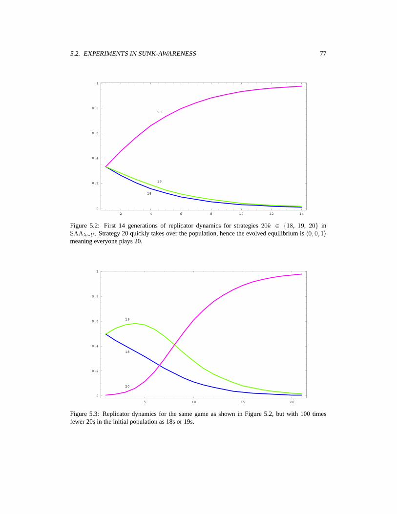
5.2. EXPERIMENTS IN SUNK-AWARENESS 77
2 4 6 8 10 12 14
0
0.2
0.4
0.6
0.8
1
18
19
20
Figure 5.2: First 14 generations of replicator dynamics for strategies 20k ∈ {18, 19, 20} inSAAλ∼U . Strategy 20 quickly takes over the population, hence the evolved equilibrium is 〈0, 0, 1〉meaning everyone plays 20.
5 10 15 20
0
0.2
0.4
0.6
0.8
1
18
19
20
Figure 5.3: Replicator dynamics for the same game as shown in Figure 5.2, but with 100 timesfewer 20s in the initial population as 18s or 19s.

78 CHAPTER 5. SIMULTANEOUS ASCENDING AUCTIONS
0 20 40 60 80 100
0
0.1
0.2
0.3
0.4
0.5
0.6
0.7
16
17
18
1920
Figure 5.4: Replicator dynamics for strategies 20k ∈ {16, . . . , 20} in SAAλ=2. The evolved Nashequilibrium is 〈0.745, 0.255, 0, 0, 0〉.
was unable to determine whether the equilibrium is unique. From this configuration, the exponen-tial model yields an observed equilibrium distribution for k intermediate between the uniform andconstant models.
Varying Number of Players
The experiments reported above all employ a five-player game configuration. We have performedfurther trials varying the number of agents (n = 2, 8, 10), maintaining the other game parameters asin our standard setup, under the exponential valuations model (Section 5.2). The objective of thisvariation was to exercise the methodology on a range of settings of game shapes, and to identify anysystematic relation between n and the equilibria we find.
Two Agents
With only two players, we can consider a larger set of candidate strategies. We investigated 14strategies, defined by the set 20k ∈ {0, 3, 6, 8, 10, 11, . . . , 17, 18, 20}. This yields 105 profiles, foreach of which we simulated 1.2 million games to construct the payoff matrix, depicted in Figure 5.7.Replicator dynamics (shown in Figure 5.8) finds a Nash equilibrium in which all agents play 15.GAMBIT identifies this as one of three equilibria (all symmetric) for this payoff matrix. All playing14 is also an equilibrium, as is the mixed strategy of playing 14 with probability 0.514 and 15otherwise. Only strategies 14, 15, and 16 survive iterated elimination of dominated strategies. Wesee in Figure 5.8 that these are indeed the three most tenacious strategies under our replicationprocess.

5.2. EXPERIMENTS IN SUNK-AWARENESS 79
0 100 200 300 400 500 600
0
0.2
0.4
0.6
0.8
1
08
12
16
20
Figure 5.5: Replicator dynamics for strategies 20k ∈ {0, 8, 12, 16, 20} in SAAλ=2. The evolvedequilibrium is 〈0, 0, 0, 1, 0〉—i.e., everyone play 16.
0 20 40 60 80 100
0
0.2
0.4
0.6
0.8
16
17
18
19
20
Figure 5.6: Replicator dynamics for strategies 20k ∈ {16, . . . , 20} in SAAλ∼E . The evolvedequilibrium is 〈0, 1, 0, 0, 0〉—i.e., everyone play 17.

80 CHAPTER 5. SIMULTANEOUS ASCENDING AUCTIONS
Strategy Profiles
11.2
11.4
11.6
11.8
12
12.2
12.4
Expected Payoff
Figure 5.7: Payoff matrix for two-player SAAλ∼E with strategies 20k ∈ {0, 3, 6, 8, 10, 11, . . . , 17,18, 20}.
0 100 200 300 400 500 600
0
0.2
0.4
0.6
0.8
0 3 6 8 1011 1213
14
15
16
1718 20
Figure 5.8: Replicator dynamics for two-player SAAλ∼E with strategies 20k ∈ {0, 3, 6, 8, 10, 11,. . . , 17, 18, 20}.

5.3. SENSITIVITY ANALYSIS FOR SUNK-AWARENESS RESULTS 81
Eight and Ten Agents
In this chapter we do not pursue the variance reduction or player reduction techniques of Chapter 3(the experiments here predate our discovery/development of those techniques). Thus, with morethan a handful of agents, it is not feasible to create a payoff matrix with more than a handful ofstrategies. Our experiments with eight and ten-player games employ a pool of four strategies: 20k ∈{10, 14, 17, 20}. This yields 165 profiles for the eight-player case, for which we simulated 1.5million games per profile. For the ten-player case there are 286 profiles. We simulated 3.9 milliongames per profile, which took many cpu weeks.
The conclusion for both eight and ten players is the same: 20 is a dominant strategy. In bothcases, the replicator dynamics show strategy 20 overwhelming the population within 40 generations.For the eight-player case, GAMBIT confirms that 20 is dominant (and therefore also the unique Nashequilibrium). But for ten players, the raw payoff matrix (i.e., the normal form without exploitingsymmetry) contains 10 million payoff values. GAMBIT does not exploit symmetry, and in ourinstallation, crashes trying to load this game into memory.
Discussion
In our experiments with the exponential valuation model, the equilibrium k value is monotone inthe number of agents, n. This can be explained by observing that increasing n can ameliorate theexposure problem. Consider the situation when the prices pass the threshold at which an agent stopsbidding. The presence of more competing bidders increases the likelihood that the stopped agentwill be let off the hook for its current winnings by being outbid. Therefore, it is less compelling foran agent to treat its current winnings as a sunk cost. In other words, k should be closer to 1 the moreagents there are, which is what we find here.
5.3 Sensitivity Analysis for Sunk-Awareness Results
Section 3.8 describes our methods of sensitivity analysis for assessing the quality of equilibria foundin empirical payoff matrices. For our sunk-awareness results, we focus on the method of assessingthe confidence on mixture probabilities.
We conclude that several of our results reported above are impervious to sampling noise. Thiswas determined by performing our equilibrium analysis on several thousand variants and finding thatthe equilibrium never changed. This was the case for results reported for SAAλ∼U in Section 5.2and for the SAAλ∼E games with eight and ten players reported in Section 5.2. For our other resultswe find varying amounts of sensitivity. Figures 5.9, 5.10, 5.11, and 5.12 illustrate this by showingthe cumulative distribution functions for the equilibrium proportions of each of the strategies. Thedotted vertical lines show the mean proportion for the corresponding strategy over all the variantpayoff matrices sampled.
For example, we see in Figure 5.9 that for the SAAλ=2 game reported in Section 5.2, the meanproportion of strategy 16 is identical to the proportion found for the maximum likelihood payoffmatrix (using the actual sample means) and it varies according to a near-perfect normal distribution.We also see that strategy 18, which died out for the maximum likelihood payoff matrix has a 10%chance of actually holding on to 5% of the population in equilibrium. Note that since this measureis conservative, the true equilibrium results are actually more likely to match those reported inSection 5.2 for the max-likelihood payoff matrices.
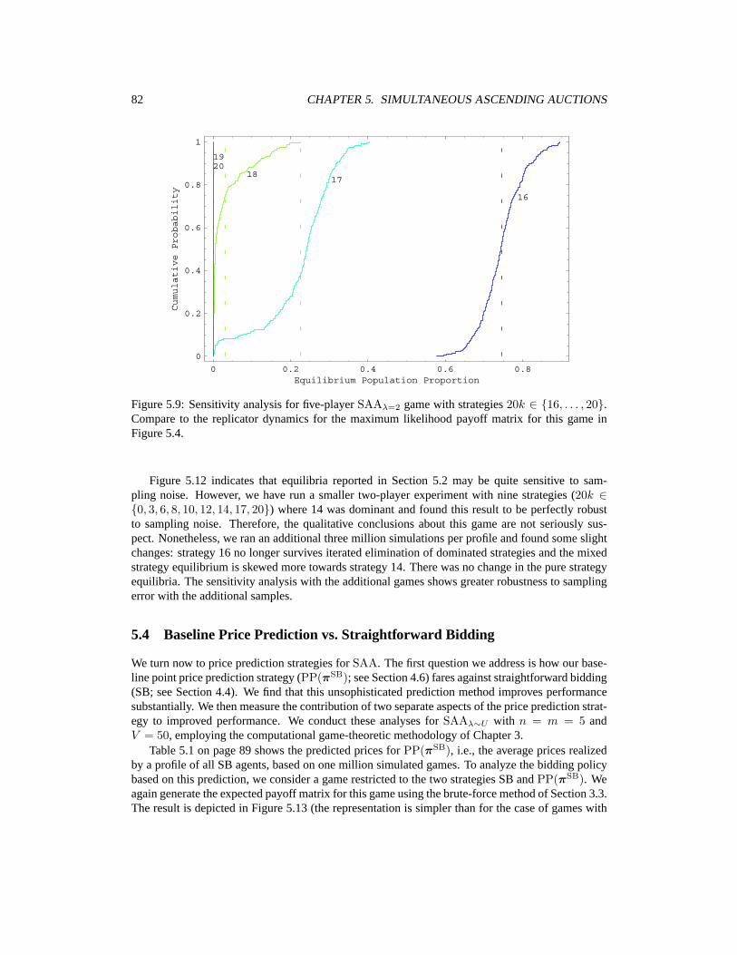
82 CHAPTER 5. SIMULTANEOUS ASCENDING AUCTIONS
0 0.2 0.4 0.6 0.8Equilibrium Population Proportion
0
0.2
0.4
0.6
0.8
1
Cumulative
Probability
16
1718
1920
Figure 5.9: Sensitivity analysis for five-player SAAλ=2 game with strategies 20k ∈ {16, . . . , 20}.Compare to the replicator dynamics for the maximum likelihood payoff matrix for this game inFigure 5.4.
Figure 5.12 indicates that equilibria reported in Section 5.2 may be quite sensitive to sam-pling noise. However, we have run a smaller two-player experiment with nine strategies (20k ∈{0, 3, 6, 8, 10, 12, 14, 17, 20}) where 14 was dominant and found this result to be perfectly robustto sampling noise. Therefore, the qualitative conclusions about this game are not seriously sus-pect. Nonetheless, we ran an additional three million simulations per profile and found some slightchanges: strategy 16 no longer survives iterated elimination of dominated strategies and the mixedstrategy equilibrium is skewed more towards strategy 14. There was no change in the pure strategyequilibria. The sensitivity analysis with the additional games shows greater robustness to samplingerror with the additional samples.
5.4 Baseline Price Prediction vs. Straightforward Bidding
We turn now to price prediction strategies for SAA. The first question we address is how our base-line point price prediction strategy (PP(πSB); see Section 4.6) fares against straightforward bidding(SB; see Section 4.4). We find that this unsophisticated prediction method improves performancesubstantially. We then measure the contribution of two separate aspects of the price prediction strat-egy to improved performance. We conduct these analyses for SAAλ∼U with n = m = 5 andV = 50, employing the computational game-theoretic methodology of Chapter 3.
Table 5.1 on page 89 shows the predicted prices for PP(πSB), i.e., the average prices realizedby a profile of all SB agents, based on one million simulated games. To analyze the bidding policybased on this prediction, we consider a game restricted to the two strategies SB and PP(πSB). Weagain generate the expected payoff matrix for this game using the brute-force method of Section 3.3.The result is depicted in Figure 5.13 (the representation is simpler than for the case of games with
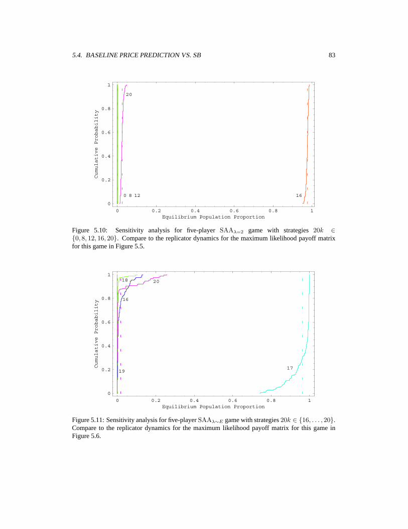
5.4. BASELINE PRICE PREDICTION VS. SB 83
0 0.2 0.4 0.6 0.8 1Equilibrium Population Proportion
0
0.2
0.4
0.6
0.8
1
Cumulative
Probability
0 8 12 16
20
Figure 5.10: Sensitivity analysis for five-player SAAλ=2 game with strategies 20k ∈{0, 8, 12, 16, 20}. Compare to the replicator dynamics for the maximum likelihood payoff matrixfor this game in Figure 5.5.
0 0.2 0.4 0.6 0.8 1Equilibrium Population Proportion
0
0.2
0.4
0.6
0.8
1
Cumulative
Probability 16
17
18
19
20
Figure 5.11: Sensitivity analysis for five-player SAAλ∼E game with strategies 20k ∈ {16, . . . , 20}.Compare to the replicator dynamics for the maximum likelihood payoff matrix for this game inFigure 5.6.
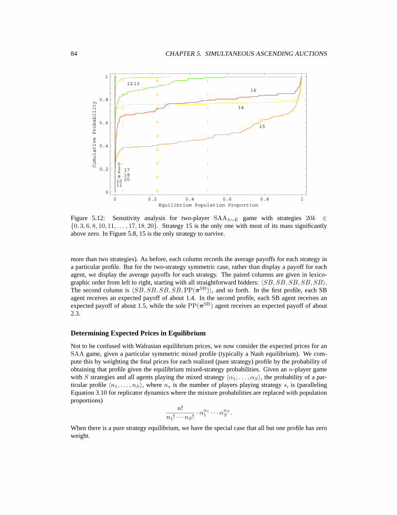
84 CHAPTER 5. SIMULTANEOUS ASCENDING AUCTIONS
0 0.2 0.4 0.6 0.8 1Equilibrium Population Proportion
0
0.2
0.4
0.6
0.8
1
Cumulative
Probability
03681011
1213
14
15
16
171820
Figure 5.12: Sensitivity analysis for two-player SAAλ∼E game with strategies 20k ∈{0, 3, 6, 8, 10, 11, . . . , 17, 18, 20}. Strategy 15 is the only one with most of its mass significantlyabove zero. In Figure 5.8, 15 is the only strategy to survive.
more than two strategies). As before, each column records the average payoffs for each strategy ina particular profile. But for the two-strategy symmetric case, rather than display a payoff for eachagent, we display the average payoffs for each strategy. The paired columns are given in lexico-graphic order from left to right, starting with all straightforward bidders: 〈SB, SB, SB, SB, SB〉.The second column is 〈SB, SB, SB, SB,PP(πSB)〉, and so forth. In the first profile, each SBagent receives an expected payoff of about 1.4. In the second profile, each SB agent receives anexpected payoff of about 1.5, while the sole PP(πSB) agent receives an expected payoff of about2.3.
Determining Expected Prices in Equilibrium
Not to be confused with Walrasian equilibrium prices, we now consider the expected prices for anSAA game, given a particular symmetric mixed profile (typically a Nash equilibrium). We com-pute this by weighting the final prices for each realized (pure strategy) profile by the probability ofobtaining that profile given the equilibrium mixed-strategy probabilities. Given an n-player gamewith S strategies and all agents playing the mixed strategy 〈α1, . . . , αS〉, the probability of a par-ticular profile 〈n1, . . . , nS〉, where ns is the number of players playing strategy s, is (parallelingEquation 3.10 for replicator dynamics where the mixture probabilities are replaced with populationproportions)
n!n1! · · ·nS !
· αn11 · · ·αnS
S .
When there is a pure strategy equilibrium, we have the special case that all but one profile has zeroweight.

5.4. BASELINE PRICE PREDICTION VS. SB 85
0 1 2 3 4 5Number of Agents Playing PP�ΠSB�
0
1
2
3
4
Average
Payoff PP
SB
Figure 5.13: Payoff matrix for the game restricted to two strategies: SB and PP(πSB). The graybars show the payoffs to SB agents and the solid bars show payoffs to predicting agents. Theprofiles are denoted by the number of predictors in the profile, from zero to five. Average payoffswere estimated from 200 thousand simulated games for each of the six profiles.
We see from inspection of the SB vs. PP(πSB) game in Figure 5.13 that PP(πSB) is a dominantstrategy since in every profile, the agents playing SB would do better switching to PP(πSB). Thusit is also the unique equilibrium. The expected final prices are then estimated simply by the averagefinal prices in this equilibrium profile: 〈11.2, 6.8, 3.8, 2.0, 0.8〉. We summarize the results for thisgame (and those in subsequent sections) in Table 5.2.
Market Efficiency with Price Predictors
In addition to considering the perspective of agents bidding in SAA, we also consider how priceprediction strategies affect market (or social) efficiency. That is, how is aggregate utility (includingthe sellers) affected by smarter strategies in SAA? The computation of efficiency for a given profileis analogous to that for determining expected prices above, using the expected efficiencies of eachrealized pure profile. The expected efficiency of a pure profile, then, is the expectation over thetype distribution of aggregate utility when the profile is played. Finally, aggregate utility of an SAAoutcome is the sum of the payoffs of the bidders plus the sum of the final prices (the payoff to thesellers).3 The optimal allocation is the assignment of goods to agents that maximizes aggregateutility. (Note that this is unaffected by prices.) When all agents play PP(πSB), market efficiencyrelative to the optimal allocation is 86%, which is 98% of the efficiency of the all-SB market. Theaverage payoff in the equilibrium profile (again computed in general by appropriate mixing of thepure-strategy payoffs) is 4.2, which is 308% of the payoff to agents in the all-SB market. Thus, ata loss of only 2% in social efficiency, agents can improve their average performance by a factor ofthree if they use a simple price prediction based on average prices in an all-SB market.
3Equivalently, aggregate utility is the sum of the values that the agents get from their bundles, not counting what theypay.

86 CHAPTER 5. SIMULTANEOUS ASCENDING AUCTIONS
Since all agents individually are better off in this equilibrium with price-predicting strategies,why is efficiency lower? The advantage to agents from using the PP(πSB) price-predicting strategyis that they reduce the number of instances in which they are left paying for goods they cannotuse (because they do not obtain their complete bundle of complementary goods). Although theexposure problem, as we showed above, can be very costly for individual agents, the allocation ofthese unused goods has no impact on social efficiency: if they are unused, it does not matter whogets the good. The payment by the agent is just a transfer to the resource seller, and our calculationof efficiency is indifferent between whether the buyer or the seller has the good or the money.Efficiency falls because to avoid the exposure problem, sometimes fewer bundles are completed,and so the allocation makes less valuable use of the available resources. In other words, priceprediction prevents spurious purchases, improving buyers’ payoffs at substantial cost to the seller,netting a slight loss in social efficiency.
5.5 How Does Price Prediction Help?
We have shown that baseline price prediction can substantially improve expected payoffs for biddingagents. We now explore the reason for the improvement: under what conditions does our price-predicting agent bid differently than SB, and how do these specific behavioral changes contribute tothe improvement in expected payoffs?
Compared to SB, our price-predicting agents use the prediction vector to modify two behaviors:choosing the best bundle of goods on which to bid, and deciding whether to participate in the biddingat all. We could of course say both behaviors manifest a single decision: on which bundle to bid,with “don’t participate” equivalent to bidding on the null bundle. We break the decision probleminto participation and bundle selection because these two decisions are qualitatively different. Wecan then assess how these two aspects of the price prediction strategy improve performance.
Participation-Only Price Prediction
In order to decompose the effects reported in the previous section into those due to changes inparticipation and those due to changes in the choice of the bundle on which to bid, we constructa new bidding strategy. Agents first calculate the best bundle on which to bid using myopicallyperceived prices, as in SB (Section 4.4). Then they choose to participate in the current round ofbidding only if surplus from that bundle, valued at the predicted, perceived prices (Equation 4.5), ispositive. The predicted prices are used only for the participation decision, and not for selecting thebest bundle on which to bid. We call this strategy PPpo(πx) where x labels an initial predictionvector.
In Figure 5.14 we present the payoff matrix for agents who choose either participation-onlyprediction, or straightforward bidding. The qualitative results for each possible strategy profile aresimilar to those in Figure 5.13. Again, the dominant (and therefore equilibrium) strategy is whenall agents play PPpo(πSB) with probability one. Expected payoff is 4.1, which is 2% lower than inthe equilibrium with full-prediction agents as described above. Relative efficiency is slightly lower(half a percentage point).
To compare participation-only prediction to full prediction more thoroughly, we compute theratio of payoff for participation-only prediction to payoff for full prediction for every possible en-vironment of agents mixing between prediction and SB. We graph the results in Figure 5.15. Thepayoff to participation-only is less than to full-prediction as long as the probability of playing SBis less than 0.32. At best, if all agents predict, participation-only prediction achieves 98.1% of the
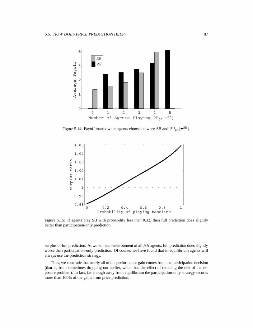
5.5. HOW DOES PRICE PREDICTION HELP? 87
0 1 2 3 4 5Number of Agents Playing PPpo�ΠSB�
0
1
2
3
4
Average
Payoff PP
SB
Figure 5.14: Payoff matrix when agents choose between SB and PPpo(πSB).
0 0.2 0.4 0.6 0.8 1Probability of playing baseline
0.98
0.99
1
1.01
1.02
1.03
1.04
1.05
Surplusratio
Figure 5.15: If agents play SB with probability less than 0.32, then full prediction does slightlybetter than participation-only prediction.
surplus of full prediction. At worst, in an environment of all SB agents, full prediction does slightlyworse than participation-only prediction. Of course, we have found that in equilibrium agents willalways use the prediction strategy.
Thus, we conclude that nearly all of the performance gain comes from the participation decision(that is, from sometimes dropping out earlier, which has the effect of reducing the risk of the ex-posure problem). In fact, far enough away from equilibrium the participation-only strategy securesmore than 100% of the gains from price prediction.
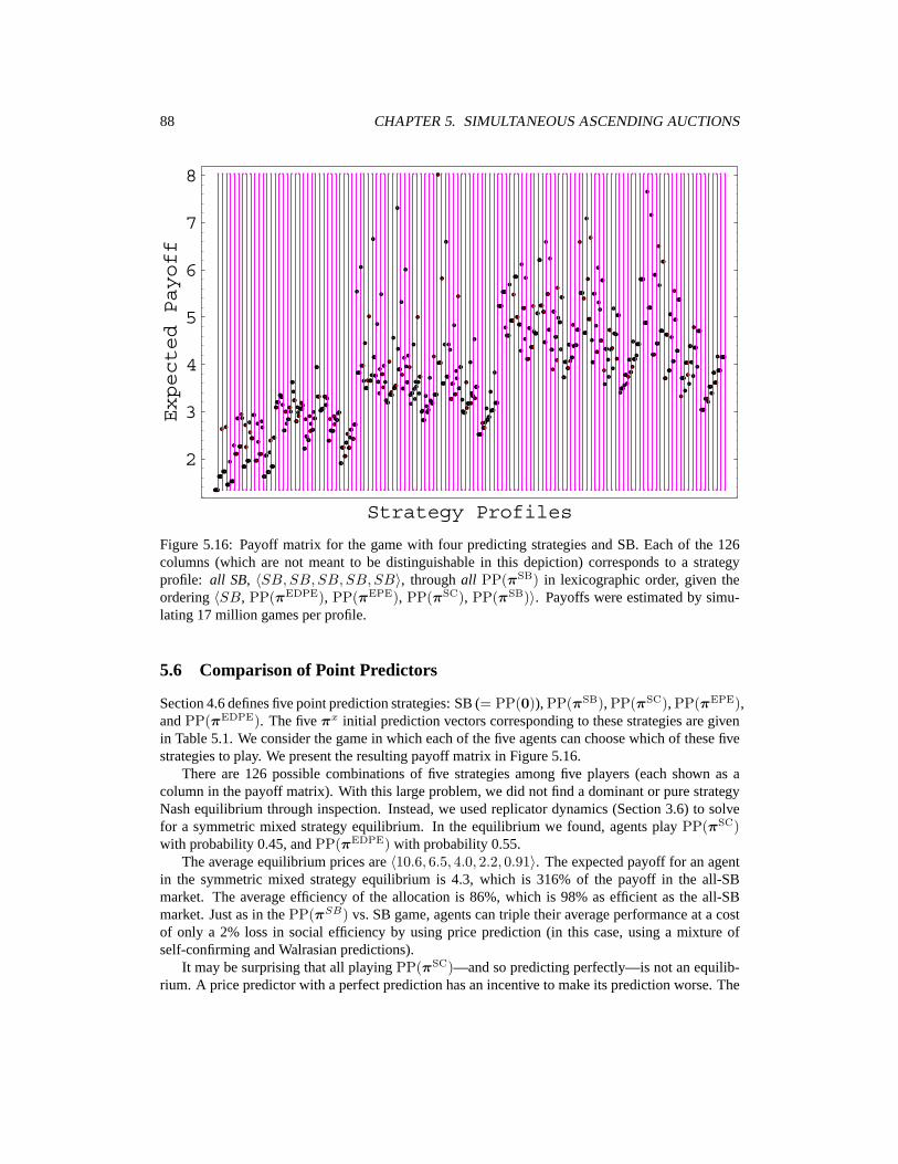
88 CHAPTER 5. SIMULTANEOUS ASCENDING AUCTIONS
Strategy Profiles
2
3
4
5
6
7
8Expected Payoff
Figure 5.16: Payoff matrix for the game with four predicting strategies and SB. Each of the 126columns (which are not meant to be distinguishable in this depiction) corresponds to a strategyprofile: all SB, 〈SB, SB, SB, SB, SB〉, through all PP(πSB) in lexicographic order, given theordering 〈SB, PP(πEDPE), PP(πEPE), PP(πSC), PP(πSB)〉. Payoffs were estimated by simu-lating 17 million games per profile.
5.6 Comparison of Point Predictors
Section 4.6 defines five point prediction strategies: SB (= PP(0)), PP(πSB), PP(πSC), PP(πEPE),and PP(πEDPE). The five πx initial prediction vectors corresponding to these strategies are givenin Table 5.1. We consider the game in which each of the five agents can choose which of these fivestrategies to play. We present the resulting payoff matrix in Figure 5.16.
There are 126 possible combinations of five strategies among five players (each shown as acolumn in the payoff matrix). With this large problem, we did not find a dominant or pure strategyNash equilibrium through inspection. Instead, we used replicator dynamics (Section 3.6) to solvefor a symmetric mixed strategy equilibrium. In the equilibrium we found, agents play PP(πSC)with probability 0.45, and PP(πEDPE) with probability 0.55.
The average equilibrium prices are 〈10.6, 6.5, 4.0, 2.2, 0.91〉. The expected payoff for an agentin the symmetric mixed strategy equilibrium is 4.3, which is 316% of the payoff in the all-SBmarket. The average efficiency of the allocation is 86%, which is 98% as efficient as the all-SBmarket. Just as in the PP(πSB) vs. SB game, agents can triple their average performance at a costof only a 2% loss in social efficiency by using price prediction (in this case, using a mixture ofself-confirming and Walrasian predictions).
It may be surprising that all playing PP(πSC)—and so predicting perfectly—is not an equilib-rium. A price predictor with a perfect prediction has an incentive to make its prediction worse. The

5.7. SELF-CONFIRMING DISTRIBUTION PREDICTORS 89
Prediction Methods Predicted Final Price VectorsSB (= PP(0)) 0 0 0 0 0PP(πSB) 14.8 10.7 7.6 4.6 1.9PP(πSC) 13.0 8.7 5.4 3.0 1.2PP(πEPE) 26.0 14.2 6.9 2.5 0.3PP(πEDPE) 20.0 12.0 8.0 2.0 0.0
Table 5.1: Price predictions for five point prediction methods applied to SAAλ∼U with n = m = 5and V = 50. Compare to realized average prices in Table 5.2.
explanation is that the predictor’s performance is a function of how it uses the price prediction, aswell as a function of its quality. In the next section we find that by using self-confirming distribu-tion prediction instead of only point predictions for final prices, an agent can further improve itsperformance.
5.7 Self-Confirming Distribution Predictors
We now analyze the performance of self-confirming distribution predictors in a variety of SAAenvironments, against a variety of other strategies.
Environments and Strategy Space
The bulk of our computational effort went into the environment—SAAλ∼U (n = m = 5, V =50)—analyzed in Sections 5.2 and 5.4. As described in Section 5.7, the empirical game for thissetting provides much evidence supporting the unique strategic stability of PP(FSC). We comple-ment this most detailed trial with smaller empirical games for a range of other SAA environments.Altogether, we studied selected environments with uniform, exponential, and fixed distributions fordesired bundle size; and agents in 3 ≤ n ≤ 8; goods in 3 ≤ m ≤ 7.
To varying degrees, we analyzed the interacting performance of 53 different strategies. Thesewere drawn from the three strategy families described in Chapter 4: sunk-aware, point predictor,and distribution predictor. For each family we varied a defining parameter to generate the differentspecific strategies. Appendix D describes the details of these 53 strategies. We chose the strategieswe deemed most promising but make no claim that we covered all reasonable variations. Ouremphasis is on evaluating the performance of PP(FSC) in combination with the other strategies.One of the noteworthy alternatives is PP(F SB), which employs the price distribution predictionformed by estimating an empirical distribution of prices resulting from all agents playing SB.
In summary, we considered:
• 21 sunk-aware strategies, including SB (k = 1): 20k ∈ {0, . . . , 20}.• 13 point predictors, by varying the method used to generate the initial prediction vector. This
includes a strategy that predicts all prices at∞, meaning it never bids unless its desired bundlesize (λ) is one.
• 19 distribution predictor strategies, by varying the method used to generate the distributionprediction. This includes degenerate and Gaussian distributions based on point predictionvectors (details in Appendix D).

90 CHAPTER 5. SIMULTANEOUS ASCENDING AUCTIONS
Gam
es(i.e.,strategy
sets)E
quilibriumProfiles
%E
ff.Payoff
Average
FinalPriceV
ectors{SB
,PP
(πSB)}
allPP
(πSB)
864.15
11.26.8
3.82.0
0.77{SB
,PP
po (π
SB)}
allPP
po (π
SB)
854.07
11.86.9
3.71.7
0.58{SB
,PP
(πSC)}
allPP
(πSC)
883.05
13.08.7
5.43.0
1.17{SB
,PP
(πSB),P
P(π
SC),P
P(π
EPE),P
P(π
ED
PE)}
0.45SC
,0.55E
DPE
864.25
10.66.5
4.02.2
0.91A
dditionalProfilesallSB
871.35
14.810.7
7.64.6
1.90allP
P(π
EPE)
745.80
4.72.1
1.71.2
0.55allP
P(π
ED
PE)
835.24
8.14.5
2.71.6
0.70
Table5.2:
Average
finalprice
vectorsin
SAA
λ∼U
(n=m
=5
andV
=50),percent
allocationefficiency
relativeto
theglobal
optimum
,and
averagepayoff
forthe
(symm
etric)equilibria
ofseveralrestricted
games
asw
ellasfor
other,non-equilibriumprofiles.P
Ppo (π
SB)
refersto
participation-onlyprediction
(seeSection
5.5)using
thebaseline
predictionvector.
Sensitivityanalysis
(Section3.8)
confirms
thatall
equilibriumresults
arerobustto
sampling
noise,andallreported
efficienciesand
payoffshave
verysm
allerrorbars.

5.7. SELF-CONFIRMING DISTRIBUTION PREDICTORS 91
With 53 strategies and five agents there are a daunting number of profiles:(n+S−1
n
)=(575
)> 4 million. Using the brute-force method (Section 3.3) of estimating the expected payoffs foreach profile by running millions of simulations of the auction protocol, estimating the entire payofffunction is infeasible. However, it is straightforward to estimate the complete payoff matrix forvarious subsets of the 53 strategies. And as we describe below, we do not need the full payoffmatrix to reach conclusions about equilibria in the 53-strategy game.
Analysis of SAAλ∼U with Five Agents and Five Goods
The largest empirical SAA game we have constructed is for the SAA environment with five agents,five goods, and the uniform valuations model. We have estimated payoffs for 4916 strategy profiles,out of the 4.2 million distinct combinations of 53 strategies. Payoff estimates are based on anaverage of 10 million samples per profile (though some profiles were simulated for as few as 200thousand games, and some for as many as 200 million). Despite the sparseness of the estimatedpayoff function (covering only 0.1% of possible profiles), we obtained several results.
First, we conjectured that the self-confirming distribution predictor strategy, PP(F SC), wouldperform well. We directly verified this: the profile where all five agents play a pure PP(FSC)strategy is a Nash equilibrium in the game restricted to 53 strategies. No unilateral deviation to anyof the other 52 pure strategies is profitable. To verify a pure-strategy symmetric equilibrium (allagents playing s) for n players and S strategies, one needs payoffs for only S profiles: one for eachstrategy playing with n − 1 copies of s. The symmetric profile is an equilibrium if there are noprofitable deviation profiles (i.e., obtained by changing the strategy of one player to obtain a higherpayoff given the others).
The fact that PP(F SC) is pure symmetric Nash for this game does not of course rule out theexistence of other Nash equilibria. Indeed, without evaluating any particular profile, we cannoteliminate the possibility that it represents a (non-symmetric) pure-strategy equilibrium itself. How-ever, the profiles we did estimate provide significant additional evidence, including the eliminationof broad classes of potential symmetric mixed equilibria.
Let us define a strategy clique as a set of strategies for which we estimated payoffs for all com-binations. Each clique defines a subgame, for which we have complete payoff information. Withinour 4916 profiles we have eight maximal cliques, all of which include strategy PP(FSC).4 Foreach of these subgames, PP(F SC) is the only strategy that survives iterated elimination of (strictly)dominated (pure) strategies.5 It follows that PP(F SC) is the unique (pure or mixed strategy) Nashequilibrium in each of these clique games. We can further conclude that in the full 53-strategy gamethere are no mixed strategy equilibria with support contained within any of the cliques, other thanthe special case of the pure-strategy PP(F SC) equilibrium.
We can show that PP(F SC) is the only small-support mixed strategy, among the two-strategycliques for which we have calculated payoffs, that is even an approximate equilibrium. Of the(522
)= 1326 pairs of strategies not including PP(F SC), we have all profile combinations for 46.
For these we obtained a lower bound of 0.32 on the value of ε (Section 3.1) such that a mixtureof one of these pairs constitutes an ε-Nash equilibrium. In other words, for any symmetric profiledefined by such a mixture, an agent can improve its payoff by a minimum of 0.32 through deviating
4One clique is a 10-strategy game with 2002 unique profiles; three are 5-strategy games (126 profiles each); one is a4-strategy game (56 profiles); and three are 3-strategy games (21 profiles).
5Even better, PP(FSC) is a dominant strategy in three of the subgames (two 3-strategy subgames and the one 5-strategysubgame in which it appears).
92 CHAPTER 5. SIMULTANEOUS ASCENDING AUCTIONS
to some other pure strategy. For reference, the payoff for the all-PP(F SC) profile is 4.51, so thisrepresents a nontrivial difference.
Finally, for each of the 4916 evaluated profiles, we can derive a bound on the ε rendering theprofile itself an ε-Nash pure-strategy equilibrium. The three most strategically stable profiles bythis measure (i.e., lowest potential gain from deviation, ε) are:
1. all PP(F SC): ε = 0 (confirmed Nash equilibrium)
2. one PP(F SB), four PP(F SC): ε > 0.13
3. two PP(F SB), three PP(F SC): ε > 0.19
The remaining profiles have ε > 0.25.Our conclusion from these observations is that PP(F SC) is a highly stable strategy within this
strategic environment, and likely uniquely so. Of course, only limited inference can be drawn fromeven an extensive analysis of only one particular SAA environment.
Self-Confirming Prediction in Other Environments
To test whether the strong performance of PP(F SC) generalizes across other SAA environments, weundertook smaller versions of this analysis on other models. Specifically, we explored 16 additionalinstances of SAA: eight each with the uniform (SAAλ∼U ) and exponential (SAAλ∼E) models(3–8 agents, 3–7 goods).6 For each we derived self-confirming price distributions (Section 4.6).We also derived price vectors and distributions for the other prediction-based strategies. For 11of the environments (eight SAAλ∼U and three SAAλ∼E), we evaluated 27 profiles: one with allPP(F SC), and for each of 26 other strategies s, one with n − 1 agents playing PP(FSC) and oneagent playing s. We ran between two and ten million games per profile in all of these environments.
For each of these 11 models, we identified the seven best responses to others playing PP(FSC)(which invariably included PP(F SC) itself). To economize on simulation time, for the other fiveSAAλ∼E environments we used the seven best responses found for the most similar of the simulatedSAAλ∼E environments. We then evaluated all profiles involving these strategies (i.e., a 7-clique) ineach of the 16 environments, based on at least 340,000 samples per profile.
We summarize our results in Table 5.3. We report the percentage gain for a participant thatdeviates from all-PP(F SC) to the best of the 26 other strategies, i.e., ε%
(PP(F SC)
)(Defini-
tion 3.2). The next two columns report sensitivity information about this figure (see Section 3.8).We show the mean ε percentage, ε% (PP(F SC)) based on 30 samples from the distribution repre-senting our belief of the true expected payoff matrix. The close correspondence between ε% andε% indicates tight confidence bounds on our estimate of ε% using the maximum-likelihood payoffmatrix. Additionally, we calculate the probability that all-PP(F SC) is a Nash equilibrium, i.e.,Pr(ε(PP(F SC)
)= 0
). Finally, for each environment with n ≤ 6 we use replicator dynamics
(Section 3.6) to find a mixed strategy equilibrium for the 7-clique, and report the probability that anagent plays PP(F SC) in this (generally mixed) Nash equilibrium.
In 15 out of these 16 environments, PP(F SC) was verified to be an ε-Nash equilibrium for anε less than 2% of the all-PP(F SC) payoff. That is, no single agent could gain as much as 2% bydeviating. The worst performance by PP(F SC) is in environment U(7, 8), for which a strategy
6We additionally consider [Osepayshvili et al., 2005] a model with fixed valuations (a game of complete information)specially constructed so that no self-confirming prediction exists. In this case, the PP(FSC) strategy uses its best approxi-mation to a self-confirming distribution. As expected, the strategy does poorly in this rather pathological environment.

5.8. CONCLUSION 93
SAAλ∼∗(m,n) ε%(PP(F SC)
)ε% Pr(ε = 0) Pr
(PP(F SC)
)E(3, 3) 0 0 1.00 1.00E(3, 5) 0 .09 .600 .996E(3, 8) .83 .85 0 —E(5, 3) 0 0 1.00 .999E(5, 5) 0 .01 .900 .998E(5, 8) .60 .64 0 —E(7, 3) 0 .06 .667 .992E(7, 6) .04 .10 .567 .549U(3, 3) 1.24 1.26 0 .725U(3, 5) 0 0 1.00 1.00U(3, 8) .56 .53 0 —U(5, 3) 1.35 1.35 0 .809U(5, 8) 1.59 1.62 0 —U(7, 3) .81 .84 0 .942U(7, 6) .52 .52 0 .929U(7, 8) 4.98 4.94 0 —
Table 5.3: Performance of PP(F SC) as a candidate symmetric equilibrium for various SAAλ∼U
and SAAλ∼E environments.
deviation could improve expected payoff by only 5%. Overall, we regard this as favorable evidencefor the PP(F SC) strategy across a range of SAA environments.
5.8 Conclusion
In our experiments in sunk-awareness, we found for the restricted game in which agents can chooseonly the sunk-awareness parameter, k, one regularity across SAA environments: the greater thenumber of agents, the less sunk aware an agent should be. Otherwise, the equilibrium k dependedsensitively on the SAA environment, in particular on the agent type distribution.
We then turned to the analysis of price prediction strategies and found that even a simple pointprice prediction can greatly improve performance (at a small cost in market efficiency) by avoidingthe exposure problem. In fact, we found that (at least for the environment we investigated) the binarychoice of participation or not had a greater contribution to improvement than the use of predictionsto guide choice of which goods to pursue. Still, point price prediction is a suboptimal strategy andso we considered next distribution predictors.
Our final class of trading strategies for SAA environments with complementarities place bidsbased on probabilistic predictions of final prices. Like the approach of Greenwald and Boyan[2004], our policy tackles the exposure problem head-on, by explicitly weighing the risks and ben-efits of placing bids on alternative bundles, or no bundle at all. The specific strategy generalizesthe point prediction method, and like that scheme is parameterized by the method for generatingpredictions. By explicitly conditioning on context (e.g., type distributions), such trading strategiesare potentially robust across varieties of SAA environments.
The strategy we consider most promising employs what we call self-confirming price distribu-tions. A price distribution is self-confirming if it reflects the prices generated when all agents play

94 CHAPTER 5. SIMULTANEOUS ASCENDING AUCTIONS
the trading strategy based on this distribution. Although such self-confirming distributions maynot always exist, we expect they will (at least approximately) in many environments of interest,especially those characterized by relatively diffuse uncertainty and a moderate number of agents.An iterative simulation algorithm, which we derive elsewhere [Osepayshvili et al., 2005], appearseffective for deriving such distributions.
To assess the self-confirming distribution predictor, we explore a range of sunk-aware and priceprediction strategies described in Chapter 4. Despite the infeasibility of exhaustively exploring theprofile space, our analyses support several game-theoretic conclusions. The results provide favor-able evidence for our favored strategy—very strong evidence in one environment we investigatedintensely, and somewhat less categorical evidence for a range of variant environments.
Neither the self-confirming distribution predictor nor any other strategy is likely to be univer-sally best across SAA environments. Nevertheless, our results establish the self-confirming priceprediction strategy as the leading contender for dealing broadly with the exposure problem. If agentsmake optimal decisions with respect to price distributions that turn out to reflect the true underly-ing uncertainty given the strategies and the environment, there may not be room for performing alot better. On the other hand, there are certainly areas where improvement should be possible, forexample:
• accounting for one’s own effect on prices, as in strategic demand reduction [Weber, 1997],
• incorporating price dependencies with reasonable computational effort, and
• timing of bids: trading off the risk of premature quiescence with the cost of pushing pricesup.
Exploring these opportunities is the subject of future work.

Chapter 6
Taming TAC: Searching for Walverine
IN WHICH we employ our empirical game methodology to choose the strategy for ouragent in the Trading Agent Competition travel-shopping game.
In Chapter 4 I describe key elements of our entry in the annual Trading Agent Competition(TAC). Focusing on the SAA-like subproblem of TAC hotel bidding, I describe price prediction aswell as strategic bid shading for hotels. The previous chapter applies our empirical game method-ology of Chapter 3 to the SAA game. Here we apply the methodology to TAC. A single TAC gamerequires close to eleven minutes of real time to simulate. Multiple times that amount of cpu timeis needed when all eight agents are playing parametric variations of our agent, Walverine. This isin contrast to the milliseconds or less of real and cpu time for SAA. Thus, for TAC we have hadto dig deeper into our collection of empirical game techniques. We begin with an analysis of bidshading in which we are able to estimate the full payoff matrix for a game restricted to two strate-gies: applying Walverine’s bid shading strategy vs. bidding marginal values (no shading). We thenconsider a richer parameterization of Walverine’s strategy, from which we choose 40 variations ofWalverine. Applying control variates (Section 3.4) to the TAC game to reduce the variance of thesampled payoffs we additionally apply the technique of player reduction (Section 3.5) and find thatthe 4-player and 2-player reductions of the TAC game are far more manageable and likely entaillittle loss of fidelity. I report on our use of these techniques in choosing our strategy for Walverinein TAC Travel 2005.
6.1 Preliminary Strategic Analysis: Shading vs. Non-Shading
In this section, we investigate the strategic behavior of hotel bid shading (Section 4.10) in isolationfrom other strategic elements. To evaluate this effect, we define a variant non-shading strategy im-plemented by Walverine 2002 with its optimal bidding procedure (i.e., shading) turned off. Agentsin this version bid their true (estimated) marginal values for every hotel room, based on predictedprices (Section 4.10). Our hypothesis was that this would hurt agent performance but at the sametime improve social welfare. We in fact found, in a trial of 55 games with all non-shading Walver-ines, the market achieved slightly better efficiency than all shading Walverines.1 The actual effectof varying strategy, however, will in general depend on the strategies of other agents.
1Though bid shading benefits the individual agent (by design) it degrades market efficiency because the market does notgenerally have available faithful signals of the relative value of goods to the various agents. If all agents shaded proportion-
95

96 CHAPTER 6. TAMING TAC: SEARCHING FOR WALVERINE
Strategy Profiles2600
2800
3000
3200
3400
3600
Expected Payoff
Figure 6.1: Empirical payoff matrix for shading vs. non-shading Walverine, based on roughly 100games per profile. The profile of all shaders is on the left and all non-shaders on the right.
Figure 6.1 shows the empirical payoff matrix for the 8-player, 2-strategy game in which theavailable strategies are to play Walverine’s strategy with shading on or off. Applying replicatordynamics (Section 3.6), we identify a symmetric mixed strategy equilibrium where agents shadewith probability 0.11, and refrain from shading with probability 0.89. GAMBIT (Section 2.1) wasunable to find a symmetric equilibrium after some hours of cpu time, finding only the asymmetricequilibrium in which five agents shade and three do not.
The predominance of truthful bidding in equilibrium demonstrates that this policy has advan-tages in a population with substantial shaders. It is not dominant, however, which means that as thepopulation approaches all non-shaders, there is benefit to shading. In equilibrium, the payoffs toshading and non-shading agents are the same, each a best response to the given mixture. The av-erage payoffs2 for all shading, all non-shading, and the equilibrium mixed strategy are 3339, 3155,and 3209, respectively. (The corresponding market efficiencies are 88.5%, 89.4%, and 89.2%.)Playing the equilibrium strategy results in an average payoff gain of 53 per agent per game (but aloss of 46 in social welfare compared to all non-shaders).
The above results of course apply specifically to the version of shading employed in Walverine;alternative shading policies incorporated in other agent strategies may produce varying outcomes.Nonetheless, having no basis to speculate on the strategic interaction of shading in an environmentwith non-Walverine agents, we in fact used this analysis to choose our strategy in TAC-03. Inparticular, we played the symmetric mixed strategy equilibrium of the empirical payoff matrix ofthe restricted game: shading with 0.11 probability.
ally, then the relative offer prices would still provide the relevant information to the market. In general, however, the pricereductions do not cancel out in this way, as the bidder’s optimization includes many agent-specific contextual factors. Weanalyze these and other effects on TAC market efficiency elsewhere [Wellman et al., 2003a].
2These were adjusted using a preliminary, ad hoc application of control variates, not described here, but subsumed bythe approach in Section 6.3.

6.2. WALVERINE PARAMETERS 97
Next, we consider a richer parameterization, applied to Walverine’s strategy in 2004, and the farmore extensive experimentation required to explore this parameter space.
6.2 Walverine Parameters
The full TAC strategy space includes all policies for bidding on flights, hotels, and entertain-ment over time, as a function of prior observations (including own client preferences and ticketendowments—i.e., own type). To focus our search, we restrict attention to variations on our basicWalverine strategy [Cheng et al., 2005], as originally developed for TAC-02 and refined incremen-tally for 2003, 2004, and 2005. Choosing the strategy for 2005 (after a preliminary attempt for 2004)has consisted primarily of applying our empirical game-theoretic approach to searching Walverine’sparameter space (Section 6.5).
We illustrate some of the possible strategy variations by describing some of the exposed pa-rameters. To invoke an instance of Walverine, the user supplies parameter values specifying whichversions of the agent’s modules to run, and what arguments to provide to these modules.
Flight Purchase Timing
Flight prices follow a biased random walk, as described in Section 4.7. Whereas flight prices aredesigned to increase in expectation given no information about the hidden parameter, conditional onthis parameter prices may be expected to increase, decrease, or stay constant. Walverine maintainsa distribution Pr(x) for each flight, initialized to be uniform on [-10,30], and updated using Bayes’srule given the observed perturbations Δ at each iteration: Pr(x | Δ) = αPr(x) Pr(Δ | x), whereα is a normalization constant. Given this distribution over the hidden x parameter, the expected per-turbation E[Δ′ | x] for the next iteration is simply (lb+ ub)/2, with bounds given by Equation 4.7.Averaging over the distribution for x, we have E[Δ′] =
∑x Pr(x)E[Δ′ | x].
Given a set of flights that Walverine has calculated to be in its optimal bundle of travel goods,it decides which to purchase now as a function of the expected perturbations, current holdings,and marginal flight values. On a high level, the strategy is designed to defer purchase of flightsthat are not quickly increasing, allowing for flexibility in avoiding expensive hotels as hotel priceinformation is revealed. The flight purchase strategy can be described in the form of a decisiontree as depicted in Figure 6.2. First, Walverine compares the expected perturbation (E[Δ′]) with athreshold T1, deferring purchase if the prices are not expected to increase by T1 or more. If T1 isexceeded, Walverine next compares the expected perturbation with a second higher threshold, T2,and if the prices are expected to increase by more than T2 Walverine purchases all units for thatflight that are in its best bundle (given predicted prices).
If T1 < E[Δ′] < T2, the Walverine flight delay strategy is designed to take into accountthe potential benefit of avoiding travel on high demand days. Walverine checks whether the flightconstitutes one end of a reducible trip: one that spans more than a single day. If the trip is notreducible, Walverine buys all the flights. If reducible, Walverine considers its own demand (definedby the best bundle) for the day that would be avoided through shortening the trip, equivalent to theday of an inflight, and the day before an outflight. If our own demand for that day is T3 or fewer,Walverine purchases all the flights. Otherwise (reducible and demand greater than T3), Walverinedelays the purchases, except possibly for one unit of the flight instance, which it will purchase if itsmarginal surplus exceeds another threshold, T4.
Though the strategy described above is based on sound calculations and tradeoff principles, it isdifficult to justify particular settings of threshold parameters without making numerous assumptions

98 CHAPTER 6. TAMING TAC: SEARCHING FOR WALVERINE
E[Δ′] < T1?
E[Δ′] > T2?
Reducible trip AND#clients > T3?
First ticket ANDsurplus > T4?
DELAY
DELAY
BUY
BUY
BUY
Y N
Y N
Y N
Y N
Figure 6.2: Decision tree for deciding whether to delay flight purchases.
and simplifications. Therefore we treat these as strategy parameters, to be explored empirically,along with the other Walverine parameters.
Bid Shading
Walverine’s “optimal” bidding strategy (Section 4.10) identifies, for each hotel auction, the bidvalue maximizing expected utility based on a model of other agents’ marginal value distributions.Because this optimization is based on numerous simplifications and approximations, we have addedseveral parameters to control its use.
We first introduce a shading mode parameter, with possible values {0, 1, 2, 4}. As in Section 6.1,one choice is to turn off shading altogether and bid marginal values. This corresponds to shadingmode 0. When shading mode is set to 4, Walverine bids a fixed fraction below marginal value.Another parameter, shade percentage, which only has effect if shade mode is 4, specifies this fixedfraction. There are two modes corresponding to the optimal shading algorithm, differing in how theymodel the other agents’ value distributions. In the first (shade mode 1), the distributions are derivedfrom the simple competitive model described in Section 4.10. For this mode, another parameter,shade model threshold turns off shading in case the model appears too unlikely given the pricequote. Specifically, we calculate the probability that the 16th highest bid is greater than or equalto the quote according to the modeled value distributions, and if too low we refrain from usingthe model for shading. For the second optimal shading method (shade mode 2), instead of thecompetitive model we employ empirically derived distributions keyed on the hotel closing order.
Other Parameters
Walverine predicts hotel prices based on Walrasian price equilibrium analysis (Section 4.9) andforms crude price distributions using a hedging model (Section 4.9) with outlier probability π.Originally, Walverine used a setting of 0.06 for this parameter. Setting it to zero turns off hedgingaltogether (equivalently, a degenerate distribution prediction yielding point predictions with cer-tainty).

6.2. WALVERINE PARAMETERS 99
Given a price distribution, one could optimize bids with respect to the distribution itself, or withrespect to the expected prices induced by the distribution. (The two are of course equivalent whenπ = 0.) Although the former approach is more accurate in principle, necessary compromises inimplementation render it ambiguous in practice which produces superior results [Greenwald andBoyan, 2004; Stone et al., 2003; Wellman et al., 2004]. Thus, we include a parameter controllingwhich method to apply in Walverine.
Several agent designers have reported employing priceline predictions, accounting for the im-pact of one’s own demand quantity on price. We implemented a version of the completion algo-rithm [Boyan and Greenwald, 2001] that optimizes with respect to pricelines, and included it as aWalverine option. A further parameter selects how price predictions and optimizations account foroutstanding hotel bids in determining current holdings. In one setting current bids for open hotelauctions are ignored, and in another the current hypothetical winnings are treated as actual holdings.This is the expected holdings parameter.
We choose among a discrete set of policies for trading entertainment. As a baseline, we im-plemented the strategy employed by LivingAgents in TAC-01 [Fritschi and Dorer, 2002]. We alsoapplied reinforcement learning to derive policies from scratch, expressed as functions of marginalvaluations and various additional state variables. The policy employed by Walverine in TAC-02was derived by Q-learning over a discretized state space. For TAC-03 we learned an alternativepolicy, this time employing a neural network to represent the value function. Finally, we have alsoimplemented an entertainment trading policy based on the top-scoring Whitebear agent [Vetsikasand Selman, 2003].
Agent Module Version Parameters
Beginning in 2004, a set of TAC rule changes reduced the viability of strategies dictating the earlypurchase of all flights. These changes included shortening the time delay to the first hotel closingfrom from four minutes to one, increasing the frequency of flight price perturbations to every 10seconds, and lowering the range from which these expected perturbations are drawn (we describethe current flight rules in Section 4.7 while our full description of Walverine includes the originalrules [Cheng et al., 2005]). These changes simplified the problem of inferring the value of x inpredicting future flight prices, while reducing the ex ante expected flight price perturbations. Theexpected perturbation of a flight price at time t could now even be negative given observed priceperturbations leading up to time t. Before these rule changes, gaining hotel price information wasthe only incentive to delaying flights. The rule changes for 2004 drastically reduced the cost ofgaining this information and introduced the possibility of realizing lower flight costs at later timesin the game.
To take advantage of these rule changes, we modified the flight module to maintain a distributionover the hidden parameter x based on observed price perturbations. The flight purchase algorithmdescribed above was added, generating flight purchase decisions based on the expected value ofthese perturbations. The flight module version is used to select among different implementationsof this algorithm, with newer revisions correcting errors found in early implementations. Flightversion 0 will purchase all flights in the beginning of the game, as Walverine originally did [Cheng etal., 2005]. The first implementation of the flight delay algorithm was found to have errors sufficientto render it useless and has been removed from use (flight version 1). Versions 2 and 3 implement thesame algorithm, with the latter implementation taking flight price boundary conditions into accountwhen computing expected perturbations of flight prices.

100 CHAPTER 6. TAMING TAC: SEARCHING FOR WALVERINE
Choices for the hotel bidding module are currently restricted to the the five most recent ver-sions (39–43) where newer versions both implement bug fixes and introduce new parameters andassociated behavior options. We attempt to introduce parameters such that new versions are ableto implement a strategy set that is a superset of the strategy set of older versions, where the useof multiple versions is a reflection of our failure to fully meet this goal. Version 40 increased theflight price refresh rate from every minute to every 10 seconds, and changed the way in which theT4 parameter is used. Version 42 corrected the way in which expected flight price perturbations arecalculated by taking boundary conditions into consideration. Version 41 corrected a bug introducedin version 40, and similarly version 43 corrected a bug introduced in version 42. Due to these bugs,versions 40 and 42 exhibit degraded performance with respect to the updated versions.
The entertainment trading strategies are divided into four main classes, two of which featurestrategies learned through game play and two of which are based on written descriptions of strategiesfrom other agents. Of the learned policies, version 10 employs neural networks, while strategy 11uses q-tables, both of which were trained using a combination of self-play and tournament play[Cheng et al., 2005]. Versions 14 and 15 implement corrections to versions 11 and 12, respectively,where the former versions failed to transmit entertainment holdings to the optimization module usedby the hotel agent. Version 12 is based on the description of entertainment trading featured in TACcompetitor LivingAgents, with version 13 implementing the same correction necessary for learnedpolicies 10 and 11. Versions 16 and 17 are both based on the strategy employed by whitebear,where version 16 had severe implementation errors and was removed from use soon after beingincorporated into the strategy space.
Despite the presence of multiple unambiguously inferior strategies, we do not purge these fromour database of games (i.e., our partial payoff matrix) because strategy profiles with some poorstrategies can still prove useful in our game theoretic analysis, described below. And we have evenoccasionally been surprised to find theoretically inferior strategy performing well in our simulations.
6.3 Control Variates for the TAC Game
From the first years of the competition, we have used various client-preference adjustments forscores in TAC Travel to adjust for luck in the game, reducing variance and getting more statisticallymeaningful comparisons from fewer games. Here we present a formula derived for the latest TACTravel rules, following the method of control variates, described in Section 3.4. For TAC, the func-tion (game simulator) to which we apply control variates produces scores (payoffs) as a function ofclient preferences, other random game data, and agent strategies. Random factors in the game (Na-ture’s and agents’ types) include hotel closing order, flight prices, entertainment ticket endowment,and, most critically, client preferences. To apply the method we need to find summary measuresof the random elements of the game that correlate with score. For example, an agent whose clientshad anomalously low hotel premiums would have its score adjusted upward as a handicap. Or in agame with very cheap flight prices, all the scores would be adjusted downward to compensate. Thespecific control variables we employ are the following, for a hypothetical agent A:
• x1: Sum of A’s clients’ entertainment premiums (8·3 = 24 values). E[x1] = (0+200)·3·8 =2400.
• x2: Sum of initial flight quotes (8 values; same for all agents). E[x2] = (250 + 400)/2 · 8 =2600.

6.3. CONTROL VARIATES FOR THE TAC GAME 101
• x3: Weighted total demand: Total demand vector (for each night, the number of the 64 clientswho would be there that night if they got their preferred trips) dotted with the demand vectorfor A’s clients. E[x3] = 540.16 (see below).
• x4: Sum of A’s clients’ hotel premiums (8 values). E[x4] = (50 + 150)/2 · 8 = 800.
The expectations are determined analytically. To do this for x3 we note that a set of n clients’aggregate demand for a particular day is a random variable Zp
n with a binomial distribution wherethe probability parameter is p = p1 = 4/10 for days 1 and 4 and p = p2 = 6/10 for days 2 and 3.3
The n parameter is the number of clients in the set (8 for one agent and (8 − 1) × 8 = 56 for theremaining seven agents). E[x3] is then
2E[(Zp18 )2 + Zp1
8 ∗ Zp156 ] + 2E[(Zp2
8 )2 + Zp28 ∗ Zp2
56 ]
=2
(8 · 56p2
1 +8∑
i=0
i2(
8i
)pi1(1− p1)8−i
)+ 2
(8 · 56p2
2 +8∑
i=0
i2(
8i
)pi2(1− p2)8−i
)
=16(63p2
1 + p1 + 63p22 + p2
)=540.16.
(We confirmed this derivation via Monte Carlo sampling, which we note is a perfectly adequatemethod for estimating the expectation of a control variate in cases where we cannot derive it analyt-ically.)
Given the above, we adjust an agent’s score by subtracting
β · (x− E[x]) =4∑
i=1
βi(xi − E[xi])
where the βs are determined by performing a multiple regression from x to score using a data setconsisting of 2190 all-Walverine games. Using adjusted scores in lieu of raw scores reduces overallvariance by 22% based on a sample of 9000 all-Walverine games.
We have also estimated the coefficients based on the 107 games in the TAC Travel 2004 semi-finals and finals and have proposed these as the basis for official score adjustments for the competi-tion:
• β1 = 0.349
• β2 = −1.721
• β3 = −2.305
• β4 = 0.916
Note that we can see from these coefficients that it improves an agent’s score somewhat to haveclients with high entertainment premiums, it hurts performance to be in a game with high flightprices, it hurts to have clients that prefer long trips (particularly when other agents’ clients do aswell), and finally, having clients with high hotel premiums improves score.
Applying the score adjustment formula to the 2004 finals yields a reduction in variance of 9%.Table 6.1 shows the average raw scores and the average adjusted scores. Figure 6.3 shows the
3This follows from the client preference distribution, described in detail at http://www.sics.se/tac.
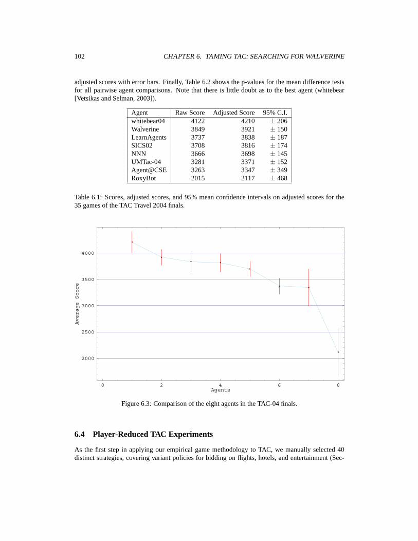
102 CHAPTER 6. TAMING TAC: SEARCHING FOR WALVERINE
adjusted scores with error bars. Finally, Table 6.2 shows the p-values for the mean difference testsfor all pairwise agent comparisons. Note that there is little doubt as to the best agent (whitebear[Vetsikas and Selman, 2003]).
Agent Raw Score Adjusted Score 95% C.I.whitebear04 4122 4210 ± 206Walverine 3849 3921 ± 150LearnAgents 3737 3838 ± 187SICS02 3708 3816 ± 174NNN 3666 3698 ± 145UMTac-04 3281 3371 ± 152Agent@CSE 3263 3347 ± 349RoxyBot 2015 2117 ± 468
Table 6.1: Scores, adjusted scores, and 95% mean confidence intervals on adjusted scores for the35 games of the TAC Travel 2004 finals.
0 2 4 6 8Agents
2000
2500
3000
3500
4000
Average Score
Figure 6.3: Comparison of the eight agents in the TAC-04 finals.
6.4 Player-Reduced TAC Experiments
As the first step in applying our empirical game methodology to TAC, we manually selected 40distinct strategies, covering variant policies for bidding on flights, hotels, and entertainment (Sec-

6.4. PLAYER-REDUCED TAC EXPERIMENTS 103
Walv. LearnA. SICS NNN UMTac Agent@CSE RoxyBotwhitebear04 0.012 0.004 0.002 0 0 0 0Walverine - 0.244 0.178 0.017 0 0.002 0LearnAgents - - 0.429 0.116 0 0.007 0SICS02 - - - 0.147 0 0.009 0NNN - - - - 0.001 0.033 0UMTac-04 - - - - - 0.449 0Agent@CSE - - - - - - 0
Table 6.2: Mean difference tests for adjusted agent scores in TAC-04 finals.
tion 6.2). The full list of strategies is presented in Table 6.3. We have collected data for a largenumber of games: over 47,000 and counting, representing over thirteen of (almost continuous) sim-ulation.4 Each game instance provides a (control variate adjusted) sample payoff vector for a profileover our restricted strategy set.
Table 6.4 shows how our dataset is apportioned among the 1-, 2-, and 4-player reduced games.We are able to exhaustively cover the 1-player game, of course. We could also have exhausted the2-player profiles, but chose to skip some of the less promising ones (29%) in favor of devotingmore samples elsewhere. The available number of samples could not cover the 4-player games, butas we see below, even 1–2% is sufficient to draw conclusions about the possible equilibria of thegame. Spread over the 8-player game, however, 47,000 instances would be insufficient to exploremuch, and so we refrain from any sampling of the unreduced game (except in the 2-strategy case inSection 6.1.)
In the spirit of hierarchical exploration, we sample more instances per profile as the game isfurther reduced, obtaining more reliable statistical estimates of the coarse background relative to itsrefinement. On introducing a new profile we generate a minimum required number of samples, andsubsequently devote further samples to particular profiles based on their potential for influencingour game-theoretic analysis. The sampling policy employed was semi-manual and somewhat adhoc, driven in an informal way by analyses of the sort described below on intermediate versions ofthe dataset. Developing a fully automated and principled sampling policy is the subject of futureresearch.
We next present the results of our analysis in the 1-, 2-, and 4-player reduced TAC games. Forthe statistical comparisons here, it is important to point out the danger of allowing the results ofstatistical significance tests to influence the number of samples, as we have done to some extant.For example, given two identical distributions, if samples are collected until a mean difference testdeclares them different at some significance level, the test will eventually spuriously succeed. Onthe other hand, it is intuitively clear that when the underlying distributions are different it is verymuch possible to sample until the difference has been established beyond doubt.
4Our simulation testbed comprises two dedicated workstations to run the agents, another RAM-laden four-CPU machineto run the agents’ optimization processes, a share of a fourth machine to run the TAC game server, and background processeson other machines to control the experiment generation and data gathering.
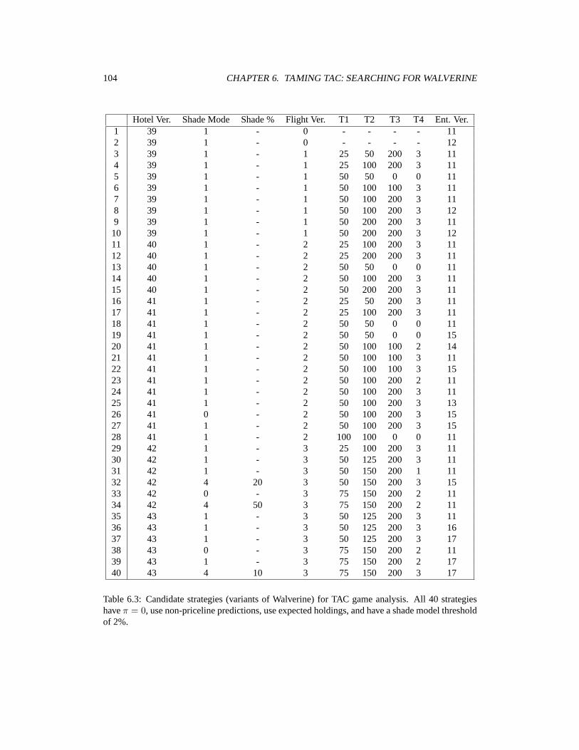
104 CHAPTER 6. TAMING TAC: SEARCHING FOR WALVERINE
Hotel Ver. Shade Mode Shade % Flight Ver. T1 T2 T3 T4 Ent. Ver.1 39 1 - 0 - - - - 112 39 1 - 0 - - - - 123 39 1 - 1 25 50 200 3 114 39 1 - 1 25 100 200 3 115 39 1 - 1 50 50 0 0 116 39 1 - 1 50 100 100 3 117 39 1 - 1 50 100 200 3 118 39 1 - 1 50 100 200 3 129 39 1 - 1 50 200 200 3 11
10 39 1 - 1 50 200 200 3 1211 40 1 - 2 25 100 200 3 1112 40 1 - 2 25 200 200 3 1113 40 1 - 2 50 50 0 0 1114 40 1 - 2 50 100 200 3 1115 40 1 - 2 50 200 200 3 1116 41 1 - 2 25 50 200 3 1117 41 1 - 2 25 100 200 3 1118 41 1 - 2 50 50 0 0 1119 41 1 - 2 50 50 0 0 1520 41 1 - 2 50 100 100 2 1421 41 1 - 2 50 100 100 3 1122 41 1 - 2 50 100 100 3 1523 41 1 - 2 50 100 200 2 1124 41 1 - 2 50 100 200 3 1125 41 1 - 2 50 100 200 3 1326 41 0 - 2 50 100 200 3 1527 41 1 - 2 50 100 200 3 1528 41 1 - 2 100 100 0 0 1129 42 1 - 3 25 100 200 3 1130 42 1 - 3 50 125 200 3 1131 42 1 - 3 50 150 200 1 1132 42 4 20 3 50 150 200 3 1533 42 0 - 3 75 150 200 2 1134 42 4 50 3 75 150 200 2 1135 43 1 - 3 50 125 200 3 1136 43 1 - 3 50 125 200 3 1637 43 1 - 3 50 125 200 3 1738 43 0 - 3 75 150 200 2 1139 43 1 - 3 75 150 200 2 1740 43 4 10 3 75 150 200 3 17
Table 6.3: Candidate strategies (variants of Walverine) for TAC game analysis. All 40 strategieshave π = 0, use non-priceline predictions, use expected holdings, and have a shade model thresholdof 2%.
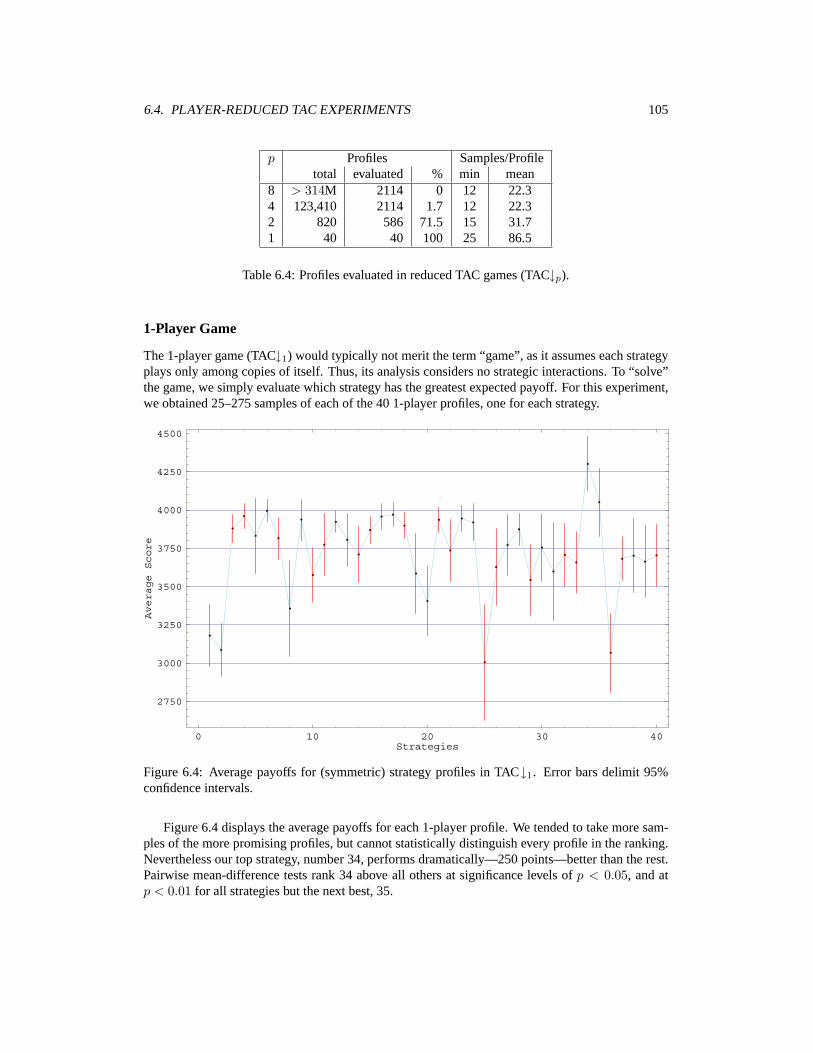
6.4. PLAYER-REDUCED TAC EXPERIMENTS 105
p Profiles Samples/Profiletotal evaluated % min mean
8 > 314M 2114 0 12 22.34 123,410 2114 1.7 12 22.32 820 586 71.5 15 31.71 40 40 100 25 86.5
Table 6.4: Profiles evaluated in reduced TAC games (TAC↓p).
1-Player Game
The 1-player game (TAC↓1) would typically not merit the term “game”, as it assumes each strategyplays only among copies of itself. Thus, its analysis considers no strategic interactions. To “solve”the game, we simply evaluate which strategy has the greatest expected payoff. For this experiment,we obtained 25–275 samples of each of the 40 1-player profiles, one for each strategy.
0 10 20 30 40Strategies
2750
3000
3250
3500
3750
4000
4250
4500
Average Score
Figure 6.4: Average payoffs for (symmetric) strategy profiles in TAC↓1. Error bars delimit 95%confidence intervals.
Figure 6.4 displays the average payoffs for each 1-player profile. We tended to take more sam-ples of the more promising profiles, but cannot statistically distinguish every profile in the ranking.Nevertheless our top strategy, number 34, performs dramatically—250 points—better than the rest.Pairwise mean-difference tests rank 34 above all others at significance levels of p < 0.05, and atp < 0.01 for all strategies but the next best, 35.

106 CHAPTER 6. TAMING TAC: SEARCHING FOR WALVERINE
In the absence of further data, we might propose strategy 34, the unique pure-strategy Nashequilibrium (PSNE) of the 1-player game. In fact, however, this strategy was designed expressly todo well against itself: it shades all hotel bids by a fixed 50% rate, resulting in very low hotel prices.The profile is quite unstable, as an agent who shades less can get much better hotel rooms, but stillbenefit from the low prices. By exploring a less extreme reduction we can start to consider some ofthe strategic interactions.
2-Player Game
The two-player game, TAC↓2, comprises 820 distinct profiles:(402
)= 780 where two different
strategies are played by four agents each, plus the 40 symmetric profiles from TAC↓1. With over70% of the profiles sampled, we have a reasonably complete description of the 2-player game,TAC↓2, among our 40 strategies. We can identify PSNE simply by examining each strategy pair(s, s′), and verifying whether each is a best response to the other. In doing so, we must account forthe fact that our sample data may not include evaluations for all possible profiles.
Definition 6.1 Profiles can be classified into four disjoint categories, defined below for the 2-playerpure-strategy case. (The generalization to n players is straightforward.)
1. If (s, s′) has not been empirically evaluated, then the estimated expected payoff u(s, s′) isundefined, and we say (s, s′) is unevaluated.
2. Otherwise, and for some t, u(t, s′) > u(s, s′) or u(t, s) > u(s′, s). In this case, we say (s, s′)is refuted.
3. Otherwise, and for some t, (t, s′) is unevaluated or (s, t) is unevaluated. In this case, we say(s, s′) is a candidate.
4. Otherwise, in which case we say (s, s′) is confirmed.
Based on our TAC↓2 simulations, we have refuted all 586 profiles for which we have estimatedpayoffs. The remaining 234 are unevaluated.
The definitions above say nothing about the statistical strength of our confirmation or refutationof equilibria. For any particular comparison, one can perform a statistical analysis to evaluate theweight of evidence for or against stability of a given profile. For example, we can construct figuresof the form of Figure 6.4, but representing the payoff in response to a particular strategy, ratherthan in self-play. Figure 6.5 shows such an example, giving the evaluated responses to strategy 34in the 2-player game. Strategy 16 is the best response in this case. When half the players deviateto strategy 16 from the all-34 profile, they improve their scores by 113 points. We can say this isan improvement, however, only at a p = 0.14 significance level. Considering the responses to 16,strategy 5 is best, but insignificantly (p = 0.47) better than the next best response, 34. Since 16 isitself a best response to 34, the refutation of (16,34) as a PSNE is statistically weak.
We can also measure the degree of refutation in terms of the ε measure (Definition 3.2). Sincethe payoff function is only partially evaluated, for any profile we have a lower bound on ε basedon the deviation profiles thus far evaluated. We can generalize the classifications above (refuted,candidate, confirmed) in the obvious way to hold with respect to any given ε level. For example,profile (16,34) is a candidate at ε = 5, but all other profiles are refuted at ε > 7. Based on the aboveanalysis of (34,34) we have that εTAC↓2(34, 34) ≥ 113. Figure 6.6 presents the distribution of εlevels at which the 586 evaluated 2-player profiles have been refuted. For example, over half have

6.4. PLAYER-REDUCED TAC EXPERIMENTS 107
0 10 20 30 40Strategies
3800
4000
4200
4400
4600
Average Score
Figure 6.5: Responses to strategy 34 in TAC↓2.
been refuted at ε > 258, and all but ten at ε > 31. These ten pure profiles remain candidates (fourof them confirmed) at ε = 27.
We can also evaluate symmetric profiles by considering mixtures of strategies. Although we donot have the full payoff function, we can derive ε bounds on mixed profiles, as long as we haveevaluated pure profiles corresponding to all combinations of strategies supported in the mixture.For example, we can derive such bounds for all 546 pairs of strategies for which we have evaluated2-player profiles. The distribution of bounds for these pairs are also plotted in Figure 6.6. Note thatthe ε bound for a strategy pair is based on the best mixture possible of that pair, and so the refu-tation levels tend to be smaller than for pure strategies. Indeed, the strategy pair (4,9) participatesin confirmed symmetric equilibrium, playing strategy 4 with probability 0.729. Another strategypair—(16,34)—is a candidate at ε = 1, and a total of 11 pairs remain candidates at eps = 10, withfive confirmed at that level.
As for the SAA experiments in Chapter 5, we apply the term k-clique to a set of k strategies suchthat all profiles involving these strategies are evaluated. A clique defines a subgame of the originalgame, which can be evaluated by standard methods. We applied iterative elimination of dominatedstrategies to all the maximal cliques of the 2-player game, ranging in size up to k = 25. This indeedpruned many strategies and induced new subsumption relations among the cliques, leaving us withonly three maximal cliques—of sizes 16–18. We applied the Lemke-Howson algorithm to thesesubgames, which identified 29 candidate symmetric equilibria (not refuted by strategies outside thecliques), with distinct supports ranging in size from two to nine. Nineteen of these mixtures areconfirmed (including the three pairs mentioned above).
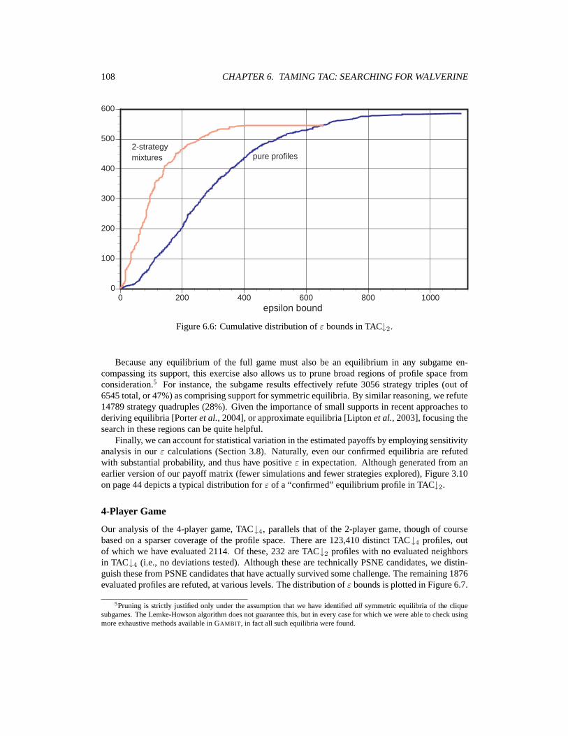
108 CHAPTER 6. TAMING TAC: SEARCHING FOR WALVERINE
0
100
200
300
400
500
600
0 200 400 600 800 1000epsilon bound
pure profiles2-strategymixtures
Figure 6.6: Cumulative distribution of ε bounds in TAC↓2.
Because any equilibrium of the full game must also be an equilibrium in any subgame en-compassing its support, this exercise also allows us to prune broad regions of profile space fromconsideration.5 For instance, the subgame results effectively refute 3056 strategy triples (out of6545 total, or 47%) as comprising support for symmetric equilibria. By similar reasoning, we refute14789 strategy quadruples (28%). Given the importance of small supports in recent approaches toderiving equilibria [Porter et al., 2004], or approximate equilibria [Lipton et al., 2003], focusing thesearch in these regions can be quite helpful.
Finally, we can account for statistical variation in the estimated payoffs by employing sensitivityanalysis in our ε calculations (Section 3.8). Naturally, even our confirmed equilibria are refutedwith substantial probability, and thus have positive ε in expectation. Although generated from anearlier version of our payoff matrix (fewer simulations and fewer strategies explored), Figure 3.10on page 44 depicts a typical distribution for ε of a “confirmed” equilibrium profile in TAC↓2.
4-Player Game
Our analysis of the 4-player game, TAC↓4, parallels that of the 2-player game, though of coursebased on a sparser coverage of the profile space. There are 123,410 distinct TAC↓4 profiles, outof which we have evaluated 2114. Of these, 232 are TAC↓2 profiles with no evaluated neighborsin TAC↓4 (i.e., no deviations tested). Although these are technically PSNE candidates, we distin-guish these from PSNE candidates that have actually survived some challenge. The remaining 1876evaluated profiles are refuted, at various levels. The distribution of ε bounds is plotted in Figure 6.7.
5Pruning is strictly justified only under the assumption that we have identified all symmetric equilibria of the cliquesubgames. The Lemke-Howson algorithm does not guarantee this, but in every case for which we were able to check usingmore exhaustive methods available in GAMBIT, in fact all such equilibria were found.

6.4. PLAYER-REDUCED TAC EXPERIMENTS 109
0
200
400
600
800
1000
1200
1400
1600
1800
2000
0 200 400 600 800 1000 1200epsilon bound
0
25
50
75
100
125
1500 40 80 120 160 200 240 280 320 360
Figure 6.7: Cumulative distribution of ε bounds in TAC ↓4. Main graph: pure profiles. Inset:2-strategy mixtures.
Figure 6.7 also shows, inset, the distribution of ε bounds over the 145 strategy pairs for whichwe have evaluated all combinations in TAC↓4 (i.e., the 2-cliques). Among these are one candidateequilibrium, and another seven at ε = 5—two of them nearly confirmed. The TAC↓4 cliques arerelatively small: three 5-cliques, 16 4-cliques, and 59 3-cliques. Eliminating dominated strategiesprunes little in this case, and we have been unsuccesful in getting GAMBIT to solve any k-cliquegames in the 4-player game for k > 2. However, applying replicator dynamics (Section 3.6) pro-duces sample symmetric subgame equilibria, including several mixture triples that constitute candi-dates with respect to the full game.
Finally, given data in both the 2-player and 4-player games, we can perform some comparisonsalong the lines of our GAMUT experiments described in Section 3.5. The results, shown in Fig-ure 6.8, are not as clear as those from the known-game experiments, in part because there is no“gold standard”, as the 4-player game is quite incompletely evaluated and the 8-player game not atall.
Discussion
Analysis of the various reduced games validates the importance of strategic interactions in TAC. Asnoted above, the best strategy in self-play (34) is not nearly a best response in most other environ-ments, though it does appear in a few mixed-strategy equilibria of TAC↓2. The strategic situationwith strategy 34 is similar to a Prisoners’ Dilemma, with 34 the “cooperate” strategy, bidding verylow prices for hotels. Defecting against such a strategy means bidding high and exploiting the lowprices at the expense of the low bidders. In fact, pairing 34 with most of the other Walverine variants

110 CHAPTER 6. TAMING TAC: SEARCHING FOR WALVERINE
♦
♦
♦
♦
♦♦
♦♦
♦
♦
♦
♦
♦
♦♦
♦
♦
♦♦♦
♦
♦♦
♦
♦
♦♦
♦
♦♦
♦
♦
♦♦
♦
♦
♦
♦
♦♦
♦
♦
♦
♦
♦
♦
♦
♦♦
♦
♦♦
♦♦
♦♦
♦
♦♦
♦♦
♦
♦
♦
♦
♦♦
♦
♦
♦
♦
♦
♦
♦
♦♦
♦
♦♦♦
♦
♦♦
♦
♦
♦♦
♦
♦♦♦♦ ♦♦
♦
♦
♦♦♦
♦
♦
♦♦
♦♦
♦ ♦
♦♦ ♦
♦♦ ♦♦ ♦
♦♦♦
♦ ♦♦ ♦
♦♦ ♦♦ ♦♦
♦
♦♦
♦ ♦♦ ♦ ♦ ♦♦♦ ♦♦♦ ♦ ♦♦0
50
100
150
200
250
300
350
400
0 50 100 150 200 250 300 350 400 450
... u
sing
bes
t 4-p
laye
r m
ixtu
re
epsilon bound in 4-player, using best 2-player mixture
Figure 6.8: ε bounds in the 4-player game achieved by playing the best mixture from the 2-playergame, versus playing the best in the 4-player. All points must be southeast of the diagonal bydefinition.
17 (D) 34 (C)17 (D) 3971 437734 (C) 3907 4302
Table 6.5: The TAC game restricted to strategies 17 and 34 constitutes a Prisoners’ Dilemma where34 is “cooperate” and 17 is “defect”. Note that the temptation payoff> reward payoff> punishmentpayoff > sucker payoff. Additionally, the reward payoff exceeds the average of the temptation andsucker payoffs.
results in a game that is isomorphic to a Prisoners’ Dilemma. This is depicted in Table 6.5 with the“defect” strategy being 17 (corresponding to Walverine-04).
Strategy 34 achieves a payoff of 4302 in self-play. For comparison:
• The top scorer in the 2004 tournament, Whitebear, averaged 4122 (adjusted to 4210).
• The best payoff we have found (so far) in TAC↓2 in a two-action mixed-strategy equilibriumcandidate (ε < 1) is 4014 (and this involves playing 34 with probability 0.12).
• The best corresponding equilibrium payoff we have found in TAC↓4 is 4018. No such equi-librium includes 34.

6.5. FINDING WALVERINE 2005 111
6.5 Finding Walverine 2005
The key question remaining after the preceding search in Walverine’s parameter space and game-theoretic analysis is: how does it inform our choice of what to play in the tournament? To do thiswe proceed in two stages:
1. Identify promising strategies in reduced games with Walverine variants.
2. Test these strategies in preliminary rounds of the tournament.
Straightforward solution of the empirical game does not yield a definitive strategy recommenda-tion since there are generally many equilibria. We do have strong evidence that all but a fraction ofthe original 40 strategies will turn out to be unstable within this set. The supports of candidate equi-libria tend to concentrate on a fraction of the strategies, suggesting we may limit consideration tothis group. Thus, we employ the preceding analysis primarily to identify promising strategies, andthen refine this set through further evaluation in preliminary rounds of the actual TAC tournament.
For the first stage—identifying promising strategies—the 1-player game is of little use. Evendiscounting strategy 34 (the best strategy in the 1-player game, specially crafted to do well withcopies of itself) our experience suggests that strategic interaction is too fundamental to TAC forperformance in the 1-player game to correlate more than loosely with performance in the unreducedgame. The 4-player game accounts for strategic interaction at a fine granularity, being sensitive todeviations by as few as two of the eight agents. The 2-player game could well lead us astray in thisrespect. For example, that strategy 34 appears in mixed-strategy equilibria in the 2-player game islikely an artifact of the coarse granularity of that approximation to TAC.
Cooperative strategies like 34 might well survive when deviations consist of half the playersin the game, but in the unreduced game we would expect them to be far less stable, i.e., not ap-pearing in any equilibrium. Nonetheless, the correlation between the 2- and 4-player game is high.Furthermore, we have a much more complete description of the 2-player game, with more statisti-cally meaningful estimates of payoffs. Finally, empirical payoff matrices for the 2-player game arefar more amenable to our solution techniques, in particular, exhaustive enumeration of symmetric(mixed) equilibria by GAMBIT. For all of these reasons, we focus on the 2-player game for choosingour final Walverine strategies, augmenting our selections with strategies that appear promising inTAC↓4.
Informally, our criteria for picking strong strategies include presence in many equilibria andhow strongly the strategy is supported. We start with an exhaustive list of all symmetric equilibriain all cliques of TAC↓2, filtered to exclude any profiles that are refuted in the full game (consideringall strategies, not just those in the cliques). There are 68 of these. We next operationalize our criteriafor promising strategies with three metrics that we can use to rank strategies given an exhaustive listof equilibria in all cliques of the 2-player game:
• Number of equilibria that the strategy is supported in.
• Maximum mixture probability with which the strategy appears.
• Sum of mixture probabilities across all equilibria.
Applying these metrics to the set of equilibria yields the strategy ranking in Table 6.6.Based on this analysis, we chose {4, 16, 17, 35} as the most promising candidates, and added
{3, 37, 39, 40} based on their promise in TAC↓4. Figure 6.9 reveals strategies 37 and 40 to be the

112 CHAPTER 6. TAMING TAC: SEARCHING FOR WALVERINE
Strategy Count Max Sum17 24 0.499 5.394 19 0.729 4.86
21 17 0.501 4.6816 18 0.892 3.7723 14 0.542 3.346 16 0.699 3.259 16 0.367 3.095 23 0.247 2.63
24 17 0.232 2.3435 15 0.641 2.0440 20 0.180 1.953 8 0.401 1.70
34 7 0.307 1.057 6 0.099 0.37
38 5 0.091 0.3539 3 0.126 0.18
Table 6.6: For all strategies appearing in an unrefuted equilibrium of a clique in TAC↓2, the numberof equilibria, the maximum mixture probability, and the sum of all mixture probabilities acrossequilibria.
top two candidates after the seeding rounds. In the semifinals we played 37 and 40 and found that37 outperformed 40, 4182 to 3945 (p = .05). Based on this, we played 37 as the Walverine strategyfor the finals in TAC-05.
6.6 TAC 2005 Outcome
Officially, Walverine placed third, based on the 80 games of the 2005 finals. However, it was clear toall present that had it not been for a network glitch that left Walverine unable to play in two games,we would have come out in first. In fact, 22 games were tainted when RoxyBot (shown in Table 6.7in second place) had a serious malfunction6 that dropped it to last place. Since games with erraticagent behavior add noise to the scores, the TAC organizers published semi-official results with theerrant RoxyBot games removed. Walverine’s missed games occurred during those games and soWalverine was (semi-officially) the top-scoring agent (Table 6.7). Figure 6.10 shows the adjustedscores with error bars. Walverine beat the runner up (RoxyBot) at the p = 0.17 significance level.Regardless of the ambiguity (statistical or otherwise) of Walverine’s victory in the competition, weconsider its strong performance under real tournament conditions to be evidence (albeit limited) ofthe efficacy of our approach to strategy generation in complex games such as TAC.
6The malfunction was actually a simple human error: instead of playing a copy of the agent on each of the two gameservers per the tournament protocol, the RoxyBot team accidentally set both copies of the agent to play on the same serverand none on the other. RoxyBot not only failed to participate in the first server’s games, but placed double bids in games onthe other server.
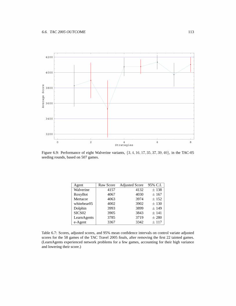
6.6. TAC 2005 OUTCOME 113
0 2 4 6 8Strategies
3200
3400
3600
3800
4000
4200
Average Score
Figure 6.9: Performance of eight Walverine variants, {3, 4, 16, 17, 35, 37, 39, 40}, in the TAC-05seeding rounds, based on 507 games.
Agent Raw Score Adjusted Score 95% C.I.Walverine 4157 4132 ± 138RoxyBot 4067 4030 ± 167Mertacor 4063 3974 ± 152whitebear05 4002 3902 ± 130Dolphin 3993 3899 ± 149SICS02 3905 3843 ± 141LearnAgents 3785 3719 ± 280e-Agent 3367 3342 ± 117
Table 6.7: Scores, adjusted scores, and 95% mean confidence intervals on control variate adjustedscores for the 58 games of the TAC Travel 2005 finals, after removing the first 22 tainted games.(LearnAgents experienced network problems for a few games, accounting for their high varianceand lowering their score.)
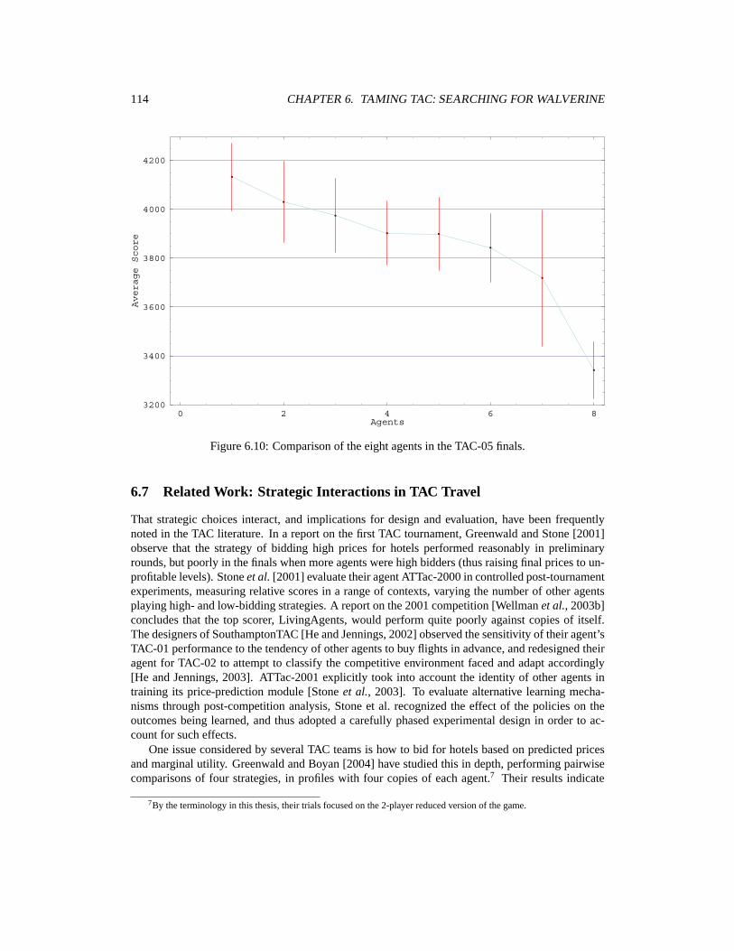
114 CHAPTER 6. TAMING TAC: SEARCHING FOR WALVERINE
0 2 4 6 8Agents
3200
3400
3600
3800
4000
4200
Average Score
Figure 6.10: Comparison of the eight agents in the TAC-05 finals.
6.7 Related Work: Strategic Interactions in TAC Travel
That strategic choices interact, and implications for design and evaluation, have been frequentlynoted in the TAC literature. In a report on the first TAC tournament, Greenwald and Stone [2001]observe that the strategy of bidding high prices for hotels performed reasonably in preliminaryrounds, but poorly in the finals when more agents were high bidders (thus raising final prices to un-profitable levels). Stone et al. [2001] evaluate their agent ATTac-2000 in controlled post-tournamentexperiments, measuring relative scores in a range of contexts, varying the number of other agentsplaying high- and low-bidding strategies. A report on the 2001 competition [Wellman et al., 2003b]concludes that the top scorer, LivingAgents, would perform quite poorly against copies of itself.The designers of SouthamptonTAC [He and Jennings, 2002] observed the sensitivity of their agent’sTAC-01 performance to the tendency of other agents to buy flights in advance, and redesigned theiragent for TAC-02 to attempt to classify the competitive environment faced and adapt accordingly[He and Jennings, 2003]. ATTac-2001 explicitly took into account the identity of other agents intraining its price-prediction module [Stone et al., 2003]. To evaluate alternative learning mecha-nisms through post-competition analysis, Stone et al. recognized the effect of the policies on theoutcomes being learned, and thus adopted a carefully phased experimental design in order to ac-count for such effects.
One issue considered by several TAC teams is how to bid for hotels based on predicted pricesand marginal utility. Greenwald and Boyan [2004] have studied this in depth, performing pairwisecomparisons of four strategies, in profiles with four copies of each agent.7 Their results indicate
7By the terminology in this thesis, their trials focused on the 2-player reduced version of the game.

6.7. RELATED WORK 115
that absolute performance of a strategy indeed depends on what the other agent plays.By far the most extensive experimental analysis reported for TAC Travel to date is that per-
formed by Vetsikas and Selman [2003]. In the process of designing Whitebear for TAC-02, theyfirst identified candidate policies for separate elements of the agents’ overall strategy. They thendefined extreme (boundary) and intermediate values for these partial strategies, and performed ex-periments according to a systematic and deliberately considered methodology. Specifically, for eachrun, they fix a particular number of agents playing intermediate strategies, varying the mixture ofboundary cases across the possible range. In all, the Whitebear experiments comprised 4500 pro-files, with varying even numbers of candidate strategies (i.e., profiles of the 4-player game). Theirdesign was further informed by 2000 games in the preliminary tournament rounds. This systematicexploration was apparently helpful, as Whitebear was the top scorer in the 2002 tournament. Thisagent’s predecessor version placed third in TAC-01, following a less comprehensive and structuredexperimentation process. Its successor placed third again in 2003, and regained its first-place stand-ing in 2004. Since the rules were adjusted for TAC-04, this outcome required a new regimen ofexperiments. Most recently, Whitebear placed second in 2005.


Chapter 7
Conclusion
IN WHICH we review our strategy generation techniques and consider the holy grail ofa general strategy generation engine.
This thesis presents new approaches to strategy generation and applies them to a variety of games.The key contributions are the following:
1. An algorithm to compute best-response strategies in a class of 2-player, one-shot, infinitegames of incomplete information.
2. An empirical game methodology for applying game-theoretic analysis to much larger gamesthan previously possible.
3. Theoretical and experimental evidence of the efficacy of our methodology.
4. A price-prediction approach to strategy generation in simultaneous auctions for complemen-tary goods.
5. Application of the above methods to find good strategies in complex games.
7.1 Summary of Contribution
In Chapter 2 I have presented a proof that best responses to piecewise linear strategies in a classof infinite games of incomplete information are piecewise linear. The proof is constructive andcontains a polynomial-time algorithm for finding such best responses. To my knowledge, this is thefirst algorithm for finding best-response strategies in a broad class of infinite games of incompleteinformation.
For some games, this best-response algorithm can be iterated to find Bayes-Nash equilibria. Itremains a goal to characterize the class of games for which iterated best response converges. Ourmethod confirms known equilibria from the literature (e.g., auction games such as FPSB, Vickrey,and bargaining), confirms an equilibrium I derive here (in the Supply Chain game), and discoversequilibria in new games (the Shared Good auction and the Joint Purchase auction).
Chapter 3 presents our empirical game methodology. I am not the first to present the core ideaof estimating a restricted form of a complex game via Monte Carlo simulation (see Section 3.9) but
117
118 CHAPTER 7. CONCLUSION
this thesis contributes several new innovations. Most notable is the approach of player reduction(Section 3.5) for which I demonstrate the potential for vast computational savings. Furthermore, Ipresent theoretical and empirical results establishing its soundness as an approximation method incertain games. Also in Chapter 3 I describe standard variance reduction techniques, showing how toframe game simulation to be amenable to their application. I present results establishing the valueof control variates applied to the First-Price Sealed-Bid Auction game (FPSB).
Next in Chapter 3 I consider the problem of finding equilibria in empirically estimated payoffmatrices. To some extent this is addressed by off-the-shelf solvers (notably GAMBIT). For thisproblem, the key contribution in this thesis is the application of replicator dynamics to findingequilibria in large games. Elsewhere in the literature, replicator dynamics is, to my knowledge,treated exclusively in terms of the equilibrium selection problem. I discuss game solution methodsin detail in Section 3.6. Finally, given an equilibrium in an empirical game, I present new methodsfor assessing the quality of the solution with respect to the full game by defining a belief distributionover payoff matrices for the underlying game (Section 3.8).
Chapter 4 lays out a general approach to generating candidate strategies in games involving bid-ding for complementary goods in simultaneous auctions: price prediction. In this chapter I describetwo games—the Trading Agent Competition (TAC) travel-shopping game and the Simultaneous As-cending Auctions (SAA) mechanism—and present families of strategies that are applicable in both.Borne out in the studies in the remaining chapters is the conjecture that price prediction is a funda-mental strategic issue in both TAC and SAA. I describe the key concept of distribution predictionin these domains and consider various ways to generate price distributions. In particular, I consider(1) the model-based approach of Walrasian price equilibrium prediction and (2) self-confirmingpredictions, a prediction strategy defined such that in equilibrium it will be correct. Additionally,I describe a new performance-based measure of prediction quality and discuss the results of itsapplication in TAC. With both the performance-based measure and an absolute accuracy measure(Euclidean distance from actual prices) I demonstrate the power of price prediction based on eco-nomic models. Even more compelling, using self-confirming distributions, prediction accuracy isby definition probabilistically perfect.
Chapter 5 presents the application of our empirical game methodology to the SAA game. I firstdescribe the type distributions we employ, defining a set of SAA environments. I then consider threefamilies of strategies in turn, performing restricted game analysis in each for various environments.For strategies parameterized by sunk-awareness (Sections 4.4 and 5.2) we find that good settings ofthis parameter depend sensitively on the SAA environment but that the equilibrium parameter settingvaries predictably with the number of agents in the game. I next consider basic price predictors,demonstrating a marked improvement over our benchmark strategy, straightforward bidding (SB). Ialso analyze the nature of the performance improvement and the effect on market efficiency. Finally,I consider self-confirming distribution prediction and show that it is a good strategy (based on theε-equilibrium measure) in a range of SAA environments.
Chapter 6 parallels Chapter 5 in applying Chapter 3’s methodology to a family of strategiesdefined in Chapter 4. In particular, I present parametric variants of our TAC entrant, the Walrasianprice predictor, Walverine. After a massive year-long simulation effort, we have estimated a partialpayoff matrix for the TAC game from which we have been able to gain sufficient strategic insight tohelp choose our strategy for the 2005 competition, with huge success.

7.2. FUTURE WORK 119
7.2 Future Work
A key question which I have only begun to address is: how well and under what circumstances willour methods succeed? The approaches in this thesis can approximate an equilibrium in the case thatthe restricted strategy space contains that equilibrium. For many simple games this is not hard toensure. It is then also often possible to confirm the equilibrium of the restricted game in the full(or less restricted) game. For games of the complexity of TAC, although our methods representthe state of the art, we have no reason to believe that our set of candidate strategies contains a trueequilibrium. Although our chosen strategy performs well (arguably the most competent strategyin the 2005 competition) it is difficult to conclude much about our empirical methodology in suchcomplex domains. Future work should more thoroughly characterize the class of games to whichthis empirical game-approximation approach is amenable.
The ultimate goal of a Strategy Generation Engine is to take as input only the description of agame (strategy sets, type distributions, and payoff function) and output Nash equilibrium strategyprofiles. Thus, another key area for future work is to take further steps toward removing the manualsteps in our current process. These include automation of the following:
1. Selection of, or search for, seed strategies for the best-response solver for infinite games, wheniterated best response does not converge from a default strategy such as truthful bidding.1
2. Generation of candidate strategies from which to generate empirical payoff matrices, in gameswith strategy spaces more complex than one-dimensional functions from type to action.
3. Choice of profiles to sample when only a partial payoff matrix is possible (as in TAC).
Whether or not we succeed in all these areas, a next natural question is: What can one do with aStrategy Generation Engine? Beyond the obvious application for participants of games, our methodscan be instrumental for mechanism designers. As mechanism designers we set the rules of a gamein order to achieve various objectives like fairness and aggregate utility (i.e., market efficiency).But to assess such outcomes, we must know what the agents will do in the face of alternative gamerules. This is precisely what a strategy generator (game solver) tells us. And, as noted in Chapter 1,it often suffices to have a strategy generator that returns a single Nash equilibrium (even when thereare many) as there are good reasons to believe such an equilibrium predicts actual agent play.
In fact, this argument can be strengthened when we have control over the mechanism. A mech-anism is incentive compatible if each agent’s equilibrium strategy is to simply submit its type (e.g.,bid truthfully). Following the constructive proof of the revelation principle [Mas-Colell et al., 1995],any mechanism can be made incentive compatible by finding some equilibrium profile and thenwrapping the original mechanism in a new interface: the allowable actions are now the possibletypes and the wrapper takes the submitted types, feeding them to the equilibrium strategies to pro-duce actions for the original game. This shows that as long as other agents play a truth-tellingstrategy (submit their types) an agent can do no better than to do so as well. Thus, not only isa strategy generator instrumental in implementing a direct revelation mechanism, doing so helpsresolve the equilibrium selection problem.
Is the holy grail of a Strategy Generation Engine attainable? A fully general and fully automatedgame solver is out of reach for the foreseeable future. Nonetheless, for broad classes of games, thisthesis presents methods for strategy generation and analysis, generates strategies for specific games,and establishes them as highly successful.
1Also promising are alternatives to iterated best response such as fictitious play.

Appendix A
Proofs and Derivations
A.1 CDF of a Piecewise Uniform Distribution
Given a piecewise uniform distribution with pdf
f(x) =
⎧⎪⎪⎪⎪⎨⎪⎪⎪⎪⎩
0 if −∞ < x ≤ d2
f2 if d2 < x ≤ d3
. . .fJ−1 if dJ−1 < x ≤ dJ
0 if dJ < x ≤ +∞
it is straightforward to derive the cdf (defining f1 ≡ 0, fJ ≡ 0, d1 ≡ −∞, and dJ+1 ≡ +∞):
F (x) =
{fi · (x− di) +
i−1∑j=1
fj · (dj+1 − dj) if di < x ≤ di+1.
The expectation (not needed for our best-response algorithm) is
n−1∑i=0
fi
2(d2
i+1 − d2i ).
A.2 Proof of Theorem 2.3
We show that the following is a symmetric Bayes-Nash equilibrium when v ∈ [3/2, 3] (whichincludes the game with v = 1.55 analyzed in Section 2.4):
s(t) ={
2v/3− 1/2 if t ≤ 2v/3− 1t/2 + v/3 otherwise.
(A.1)
The expected utility (surplus) for agent type t bidding a against agent type T ∼ U [0, 1] playing
121

122 APPENDIX A. PROOFS AND DERIVATIONS
(A.1) is:
EU(t, a) = ET [u(t, a, T, s(T )]= (a− t) Pr(a+ s(T ) ≤ v)= (a− t)
[Pr(T ≤ 2v/3− 1)
·Pr(a+ 2v/3− 1/2 ≤ v | T ≤ 2v/3− 1)+ Pr(T > 2v/3− 1)
·Pr(a+ T/2 + v/3 ≤ v | T > 2v/3− 1)].
We consider three cases, conditioned on the range of a.Case 1: a ≤ 2v/3− 1/2.The expected surplus is:
EU(t, a) = (a− t)[(2v/3− 1) + (2− 2v/3)]= a− t.
Since the expected surplus is monotonic in a, the optimal bid is found at the upper boundary,namely, a = 2v/3− 1/2, giving us EU(t, a) = 2v/3− 1/2− t.
Case 2: a ∈ [2v/3− 1/2, v/3 + 1/2].The expected surplus is:
EU(t, a) =(a− t)[(2v/3− 1) + (2v/3− 2a+ 1)]=(a− t)(4v/3− 2a).
(A.2)
Equation A.2 is maximized at a = t/2 + v/3. With v ∈ [3/2 , 3], we need to consider whetherthis point occurs below the lower boundary of a. This gives us two cases. If t > 2v/3 − 1 thenthe maximum of (A.2) lies in the range of bids we consider here, and the best response is a1 =t1/2 + v/3, giving us EU(t, a) = (3t− 2v)2/18. If t > 2v/3− 1 then the maximum occurs at thelower boundary, and the best response is a = 2v/3− 1/2, giving us EU(t, a) = 2v/3− 1/2− t.
Case 3: a > v/3 + 1/2.The expected surplus is always zero in this range.
The expected surplus of Case 2 is always positive, and always at least as high as Case 1, henceit must specify the best-response policy. But Case 2 gives us the bidding policy specified by (A.1)when v ≤ 3.
We have shown that (A.1) is a best response to itself for all v ∈ [3/2, 3], hence it is a symmetricBayes-Nash equilibrium. �
A.3 Proof of Theorem 2.4
We show that the following is a Bayes-Nash equilibrium of the auction game from Section 2.4:
a(t) =2t+A
3. (A.3)

A.3. PROOF OF THEOREM 2.4 123
Given that the other agent employs the strategy in (A.3) for its type T ∼ U [0, 1], we show that(A.3) is a best response. The expected utility (surplus) for an agent playing bid a against an agentbidding according to (A.3) is
EU(t, a) = E
[u
(t, a,
2T +A
3
)]
= (t− a/2)Pr(a > s(T )) + E
[12· 2T +A
3
∣∣∣∣ a < s(T )]
Pr(a < s(T ))
= (t− a/2)Pr(
3a−A2
> T
)
+ E
[2T +A
6
∣∣∣∣ 3a−A2
< T
]· Pr
(3a−A
2< T
).
(A.4)
We consider two cases, conditioned on the range of a.
Case 1: a >2B +A
3.
The expected surplus is:
EU(t, a) = t− a/2
which implies an optimal action at the left boundary:
a∗1 =2B +A
3.
Case 2: a <2B +A
3.
In this case, both the probabilities in (A.4) are nonzero and the expected surplus is
EU(a) =(t− a/2)
3a−A2
−AB −A + 1/6
⎛⎜⎝2 ·
3a−A2
+B
2+A
⎞⎟⎠ · B −
3a−A2
B −A ,
which implies an optimal action where the derivative with respect to a is zero:
a∗2 =2t+A
3.
Comparing the expected surpluses of the candidate action functions,
EU(a∗2)− EU(a∗1) =(B − t)22(B −A)
> 0.
Therefore a∗2 is a best response to (A.3), i.e., itself, and therefore a Bayes-Nash equilibrium. �
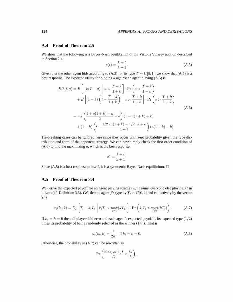
124 APPENDIX A. PROOFS AND DERIVATIONS
A.4 Proof of Theorem 2.5
We show that the following is a Bayes-Nash equilibrium of the Vicious Vickrey auction describedin Section 2.4:
a(t) =k + t
k + 1. (A.5)
Given that the other agent bids according to (A.5) for its type T ∼ U [0, 1], we show that (A.5) is abest response. The expected utility for bidding a against an agent playing (A.5) is
EU(t, a) = E
[−k(T − a)
∣∣∣∣ a < T + k
1 + k
]· Pr
(a <
T + k
1 + k
)
+ E
[(1− k)
(t− T + k
1 + k
) ∣∣∣∣ a > T + k
1 + k
]· Pr
(a >
T + k
1 + k
)
= −k(
1 + a(1 + k)− k2
− a)
(1− a(1 + k) + k)
+ (1− k)(t− 1/2 · a(1 + k)− 1/2 · k + k
1 + k
)(a(1 + k)− k).
(A.6)
Tie-breaking cases can be ignored here since they occur with zero probability given the type dis-tribution and form of the opponent strategy. We can now simply check the first-order condition of(A.6) to find the maximizing a, which is the best response:
a∗ =k + t
k + 1.
Since (A.5) is a best response to itself, it is a symmetric Bayes-Nash equilibrium. �
A.5 Proof of Theorem 3.4
We derive the expected payoff for an agent playing strategy kit against everyone else playing kt inFPSBn (cf. Definition 3.3). (We denote agent j’s type by Tj ∼ U [0, 1] and collectively by the vectorT .)
ui(ki, k) = ET
[Ti − kiTi
∣∣∣∣ kiTi > maxj �=i
(kTj)]· Pr
(kiTi > max
j �=i(kTj)
). (A.7)
If ki = k = 0 then all players bid zero and each agent’s expected payoff is its expected type (1/2)times its probability of being randomly selected as the winner (1/n). That is,
ui(ki, k) =12n
if ki = k = 0. (A.8)
Otherwise, the probability in (A.7) can be rewritten as
Pr(
maxj �=i(Tj)Ti
<ki
k
).

A.5. PROOF OF THEOREM 3.4 125
Letting r ≡ ki/k and Y ≡ maxj �=i(Tj), the cdf and pdf of Y—a random variable which is themaximum of n− 1 random variables—and Ti are
FTi(x) = x and fTi
(x) = 1 for x ∈ [0, 1] (i.e., Ti ∼ U [0, 1]);
FY (y) = yn−1 and fY (y) = (n− 1)yn−2 for y ∈ [0, 1].
We now calculate the cdf of Z ≡ Y/Ti:
FZ(r) =∫ ∞
0
∫ xr
−∞fTi
(x)fY (y) dydx
=∫ ∞
0
∫ xr
−∞(n− 1)yn−2 dydx.
Since the probability density is only positive for Ti, Y ∈ [0, 1] the integration region has twodifferent shapes depending on whether r < 1, and so the above integral is FZ(r) =
⎧⎪⎪⎪⎪⎪⎨⎪⎪⎪⎪⎪⎩
∫ 1
0
∫ xr
0
(n− 1)yn−2 dydx =rn−1
nif r < 1
∫ 1/r
0
∫ xr
0
(n− 1)yn−2 dydx+∫ 1
1/r
∫ 1
0
(n− 1)yn−2 dydx =1nr
+r − 1r
otherwise.
We can now rewrite (A.7) as
(1− ki)E [Ti | Z < r] · FZ(r). (A.9)
Let X be the random variable Ti conditionalized by Z < r, then
FX(t) = Pr(Ti < t | Z < r) =Pr(Ti < t, Z < r)
Pr(Z < r)=
Pr(Y/r < Ti < t)Pr(Z < r)
=
∫ t
0
∫ rx
0
fY (y)fTi(x) dydx
FZ(r). (A.10)
For the case r < 1, the double integral in the numerator evaluates to rn−1tn/n and the denominatorto rn−1/n, yielding
FX(t) = tn and fX(t) = ntn−1 for t ∈ [0, 1].
And so the expectation in (A.9) is
E[Ti | Z < r] =∫ 1
0
t · ntn−1 dt =n
n+ 1(for r < 1). (A.11)
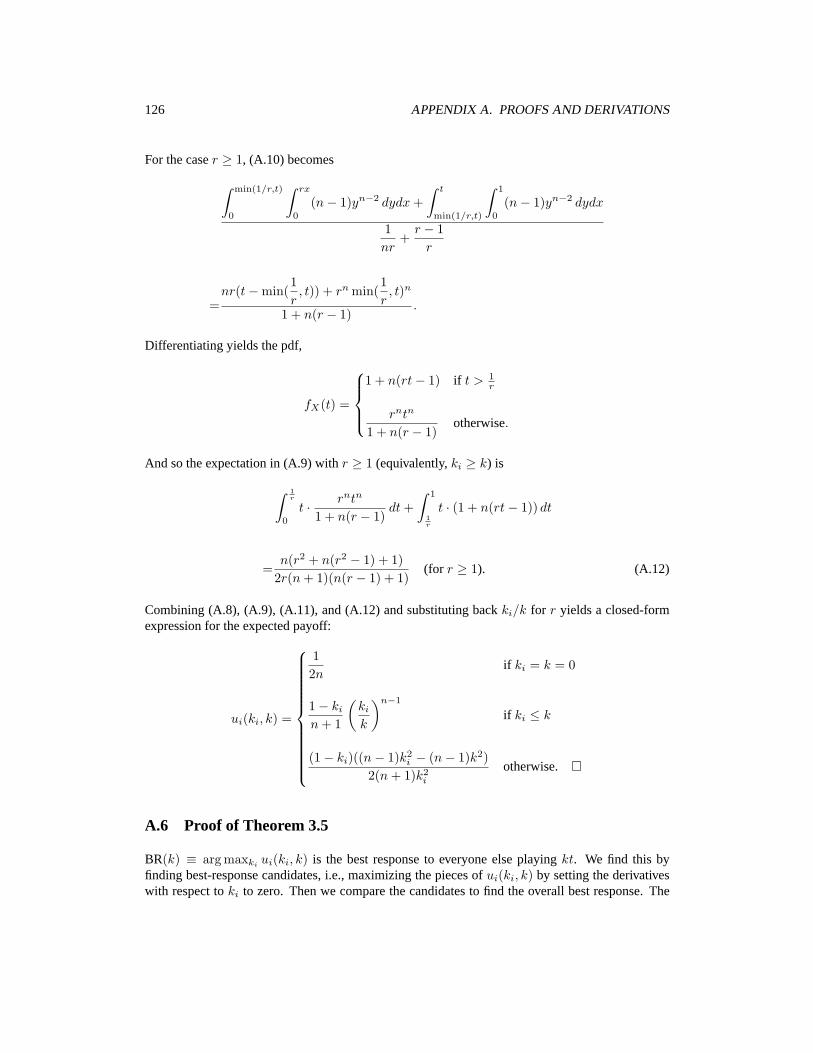
126 APPENDIX A. PROOFS AND DERIVATIONS
For the case r ≥ 1, (A.10) becomes
∫ min(1/r,t)
0
∫ rx
0
(n− 1)yn−2 dydx+∫ t
min(1/r,t)
∫ 1
0
(n− 1)yn−2 dydx
1nr
+r − 1r
=nr(t−min(
1r, t)) + rn min(
1r, t)n
1 + n(r − 1).
Differentiating yields the pdf,
fX(t) =
⎧⎪⎪⎨⎪⎪⎩
1 + n(rt− 1) if t > 1r
rntn
1 + n(r − 1)otherwise.
And so the expectation in (A.9) with r ≥ 1 (equivalently, ki ≥ k) is
∫ 1r
0
t · rntn
1 + n(r − 1)dt+
∫ 1
1r
t · (1 + n(rt− 1)) dt
=n(r2 + n(r2 − 1) + 1)
2r(n+ 1)(n(r − 1) + 1)(for r ≥ 1). (A.12)
Combining (A.8), (A.9), (A.11), and (A.12) and substituting back ki/k for r yields a closed-formexpression for the expected payoff:
ui(ki, k) =
⎧⎪⎪⎪⎪⎪⎪⎪⎪⎪⎪⎪⎨⎪⎪⎪⎪⎪⎪⎪⎪⎪⎪⎪⎩
12n
if ki = k = 0
1− ki
n+ 1
(ki
k
)n−1
if ki ≤ k
(1− ki)((n− 1)k2i − (n− 1)k2)
2(n+ 1)k2i
otherwise. �
A.6 Proof of Theorem 3.5
BR(k) ≡ arg maxkiui(ki, k) is the best response to everyone else playing kt. We find this by
finding best-response candidates, i.e., maximizing the pieces of ui(ki, k) by setting the derivativeswith respect to ki to zero. Then we compare the candidates to find the overall best response. The

A.7. PROOF OF LEMMA 3.7 127
best-response candidates for ui(ki, k), as found by Mathematica, are:
ψ ≡ n− 1n
, ξ ≡3√
3(k2(n2 − 1
) (9n+
√3(n+ 1) ((n− 1)k2 + 27(n+ 1)) + 9
))2/3
− 32/3k2(n2 − 1
)3(n+ 1) 3
√k2(n− 1)
(9n2 + 18n+ (n+ 1)3/2
√3(n− 1)k2 + 81(n+ 1) + 9
) .
We first treat the special case of k = 0. As in general FPSB with unrestricted strategies, there is nobest response to the other agents all bidding zero: the lower your bid the better as long as it’s strictlypositive. For k > 0, the condition ui(ψ, k) > ui(ξ, k) reduces to k ≥ n−1
n and so the best responseto a symmetric profile of strategy k is:
BR(k) =
⎧⎪⎪⎪⎪⎪⎪⎪⎪⎨⎪⎪⎪⎪⎪⎪⎪⎪⎩
undefined if k = 0
ξ if k <n− 1n
n− 1n
if k ≥ n− 1n
. �
A.7 Proof of Lemma 3.7
To show that f(k) has no roots in (0,+∞) except n−1n we establish a set of points guaranteed to be
a superset of the set of roots of f(k) and show that none, other than n−1n , are positive. We first apply
the following transformations to f to combine common subexpressions and make all the coefficientsintegers:1
(n− 1)k2 + 27(n+ 1)→ 3a2
n+ 1and
(9n+ 3a+ 9)(n2 − 1
)k2 → 9b3.
(A.13)
These transformations have no effect as long as
a =
√(n+ 1) ((n− 1)k2 + 27(n+ 1))
3and
b = 3
√(3a+ 9n+ 9) (n2 − 1) k2
9,
(A.14)
or, equivalently, when the following polynomials are zero:
(n+ 1)((n− 1)k2 + 27(n+ 1)
)− 3a2 and (A.15)
(3a+ 9n+ 9)(n2 − 1
)k2 − 9b3. (A.16)
1This and following key insights that made this proof possible are due to Maxim Rytin. Andrzej Kozlowski and DanielLichtblau also provided invaluable guidance.

128 APPENDIX A. PROOFS AND DERIVATIONS
(In fact, transforming an equation of the form x = y into x2 = y2 allows for additional spurioussolutions such as x = 1 and y = −1. This does not affect the proof since we need only a guaranteethat our set of possible roots is a superset of the actual roots.) After applying (A.13), simplifying(using the fact that n, a, and b are all positive), and collecting the terms over a common denominator,we can write the numerator of f(k) as
(−3b2 + 3k(n+ 1)b+ k2(n2 − 1
)) (9b4 + 9(k − 1)(n− 1)b3
− 3k(2k + 3)(n2 − 1
)b2 − 3(k − 1)k2(n− 1)2(n+ 1)b+ k4
(n2 − 1
)2) (A.17)
and the denominator as6b(n+ 1)
(k2(n2 − 1
)− 3b2)2
(A.18)
with a and b defined by (A.14).We can now find all possible roots of (A.17) given (A.14) by finding the common roots of
(A.17), (A.15), and (A.16). To do this, we apply Buchberger’s [1982] algorithm to compute aGrobner basis,2 resulting in
k8(n− 1)4(n+ 1)5(kn− n+ 1)2(nk2 − k2 + 2nk + 6k + n− 1
), (A.19)
which for n > 1 has the following real roots:{−n+ 2
√2√n+ 1 + 3
n− 1, −n− 2
√2√n+ 1 + 3
n− 1, 0,
n− 1n
}(A.20)
These comprise all the possible real roots of the numerator and so there can be no other roots off(k). (A root of the numerator is a root of the quotient unless also a root of the denominator.) Weverify directly using simplification and reduction routines in Mathematica, that f(n−1
n ) = 0 for alln > 1. This is done by establishing that the numerator of f(n−1
n ) is equal to zero for all n > 1 and,likewise, that the denominator is not.3 The numerator of f(n−1
n ) is
3√
3(n− 1)6(32/3n2 − 3νn− 3
√3((n+ 1)
(9n2 + 2μn+ 9n+ μ
))2/3 − 32/3)
·(−32/3n2 − 3νn− 3ν + 3
√3((n+ 1)
(9n2 + 2μn+ 9n+ μ
))2/3+ 32/3
)2
where
μ ≡√
3(n+ 1)(7n− 1) and
ν ≡ 3√
(n+ 1) (9n2 + 2μn+ 9n+ μ).
2Grobner bases [Becker and Weispfenning, 1993] are a generalization of Gaussian elimination to the case of polynomialsystems. The set of polynomials G comprising the Grobner basis of a set of polynomials P has the property that it shares thesame set of common roots as P . Buchberger’s algorithm is implemented in the Mathematica function GroebnerBasis.
3The following evaluating to True comprises the computer-assisted proof (with thanks yet again to Maxim Rytin):
simp = Function[x, Simplify[Together//@x, n>1]];Reduce[ForAll[n, n>1, simp@simp@Numerator@Together@f[n,(n-1)/n]]]
And similarly for the denominator.

A.8. PROOF OF THEOREM 3.10 129
The denominator is(− 3√
3n2 + ((n+ 1)(2nμ+ μ+ 9n(n+ 1)))2/3 + 3√
3)2
18(n− 1)5n(n+ 1)4/3
· 3√
2nμ+ μ+ 9n(n+ 1).
It remains to show that no other points in (A.20) are positive. The first is clearly negative. Toshow that the second is also negative it suffices to show that n+ 3− 2
√2√n+ 1 > 0 which is the
case because
n > 1
=⇒ (n− 1)2 > 0
=⇒ n2 − 2n+ 1 > 0
=⇒ n2 + 6n+ 9 > 8n+ 8
=⇒ (n+ 3)2 > 8n+ 8
=⇒ n+ 3 >√
8n+ 8
=⇒ n+ 3− 2√
2√n+ 1 > 0.
Therefore the only positive root of f(k) isn− 1n
. �
A.8 Proof of Theorem 3.10
We derive the equilibrium of FPSBn↓p by showing that the game is equivalent to a p-player FPSBgame with a particular non-uniform type distribution. Let q ≡ n/p. By the definitions of FPSBn(Definition 3.3) and of a reduced game (Definition 3.9), FPSBn↓p is a p-player game with eachplayer having multidimensional type [v1, . . . , vq], with vi ∼ U [0, 1] being the type (valuation) ofone of the original n players. The key insight for the proof is that since each of the p players inthe reduced game must play the same strategy for each of the q players it controls and since thestrategy is monotone increasing in type (specifically k · vi), then all but the greatest of the vi areirrelevant. This is because if one of the q subplayers gets positive payoff it is because it had thehighest valuation of [v1, . . . , vq]. Thus, each player’s type reduces to the maximum of q randomvariables, i.i.d. U [0, 1]. In general the cdf of the maximum of m random variables, i.i.d. with cdf Fis FMAX(x) = F (x)m. The cdf for a player’s type in FPSBn↓p is the special case, FMAX(x) = xq.
Theorem 3.1 [McAfee and McMillan, 1987] gives the unique symmetric equilibrium for FPSBwith n players having types i.i.d. with cdf F , and a lowest possible type A:
a(t) = t−
∫ t
A
F (x)n−1 dx
F (t)n−1.
Substituting FMAX for F , this gives us the equilibrium for any FPSB (with arbitrary i.i.d. typedistribution, F , with lower bound A) reduced from n to p players:
a(t) = t−
∫ t
A
F (x)n−q dx
F (t)n−q.

130 APPENDIX A. PROOFS AND DERIVATIONS
In the special case of U [A,B] types, the equilibrium is
a(t) =Ap+ n(p− 1)p+ n(p− 1)
· t.
Finally, for U [0, 1], that is, FPSBn↓p, the unique symmetric Nash equilibrium is
a(t) =n(p− 1)
p+ n(p− 1)· t. �
A.9 Proof of Lemma 3.11
Corollary 3.6 defines the function ε(k) ≡ εFPSBn(k). Since we are only concerned with the case0 < k ≤ n−1
n and since, by Lemma 3.7, the second and third cases of ε(k) are equal at k = n−1n
(namely zero) we have for 0 < k ≤ n−1n that ε(k) is equal to the continuously differentiable
function f in Lemma 3.7.To establish that f(k) is strictly decreasing in (0, n−1
n ] we first consider the roots of its deriva-tive, f ′(k). It is (computationally) easy to differentiate f but takes pages to display. As in the proofof Lemma 3.7 (Appendix A.7) we perform transformations (A.13) on f ′(k) that combine commonsubexpressions and make the coefficients integers. After applying (A.13), simplifying (using thefact that n, a, and b are all positive), and collecting the terms over a common denominator, we canwrite the numerator of f ′(k) as(n2 − 1
)6k11 + 3
(n2 − 1
)5 (b2 + 2a(a+ 3n+ 3)
)k9
+ 18b2 (a(a− 3b+ 3) + 3b+ 3(a+ b)n)(n2 − 1
)4k7 − 162ab4
(n2 − 1
)3k6
+ 27b3(n2 − 1
)3 (12(n+ 1)a2 + 18
(b2 + 2(n+ 1)2
)a+ b2(6n− b+ 6)
)k5
− 81b5(n2 − 1
)2 (b3 + 2a2(b− 6n− 6)) + 12a
(3b2 + 2(n+ 1)b− 3(n+ 1)2
))k3
+ 1458ab6(n2 − 1
)2k4 − 4374ab8
(n2 − 1
)k2
− 486ab8(n2 − 1
)(a+ 12(n− b+ 1))k + 4374ab10,
(A.21)
with a and b defined by (A.14).We can now find the roots of (A.21) given (A.14) by finding the common roots of (A.21), (A.15),
and (A.16). As in Appendix A.7 we do this by computing a Grobner basis, yielding
(n− 1)7(n+ 1)8k13(kn−n+ 1)(kn2 + n2 − kn+ 2n+ 1
) (nk2 − k2 + 27n+ 27
)(A.22)
which, for n > 1, has roots at zero,
− n2 + 2n+ 1n2 − n , and (A.23)
n− 1n
.
These comprise all the possible real roots of the numerator and so there can be no other roots off ′(k). Since (A.23) is negative and the only other possible roots are on the boundaries of (0, n−1
n ]

A.10. PROOF OF THEOREM 3.12 131
we have established that f ′(k) is nonzero in the interior of that range. Since it is also continuous itmust then be exclusively negative or positive. This implies that the original function, ε(k), is eitherstrictly increasing or strictly decreasing in (0, n−1
n ]. Since, by Lemma 3.7, f(n−1n ) = ε(n−1
n ) = 0we can show that ε(k) is not strictly increasing by showing for some k ∈ (0, n−1
n ) that f(k) > 0.It is straightforward to compute
limk→0
f(k) =n− 1
2(n+ 1)
(which is ≥ 1/6 for all n > 1). This establishes that f(k) = ε(k) decreases somewhere in(0, n−1
n ]. And since it never changes direction—being continuous and its derivative having noroots in (0, n−1
n )—it must be strictly decreasing. �
A.10 Proof of Theorem 3.12
Theorem 3.10 and Theorem 3.8 give us the unique symmetric equilibria of FPSBn↓p and FPSBn soit suffices to show that
p− 1p
<n(p− 1)
p+ n(p− 1)<n− 1n
.
Consider first the left inequality:
p < n
=⇒ p− n < 0=⇒ p+ np− n < np
=⇒ p+ n(p− 1) < np
=⇒ 1 <np
p+ n(p− 1)since n, p ≥ 1 =⇒ p+ n(p− 1) > 0
=⇒ p− 1 <np(p− 1)p+ n(p− 1)
=⇒ p− 1p
<n(p− 1)
p+ n(p− 1).
Similarly for the second inequality,
p < n
=⇒ 0 < n− p=⇒ pn2 − n2 < n− p+ pn2 − n2
=⇒ n2(p− 1) < (n− 1)(p+ n(p− 1))
=⇒ n(p− 1)p+ n(p− 1)
<n− 1n
since n and p+ n(p− 1) are both > 0. �
A.11 Proof of Theorem 3.13
Theorem 3.12 and Lemma 3.11 establish all of Theorem 3.13 except that
n(q − 1)q + n(q − 1)
<n(p− 1)
p+ n(p− 1)
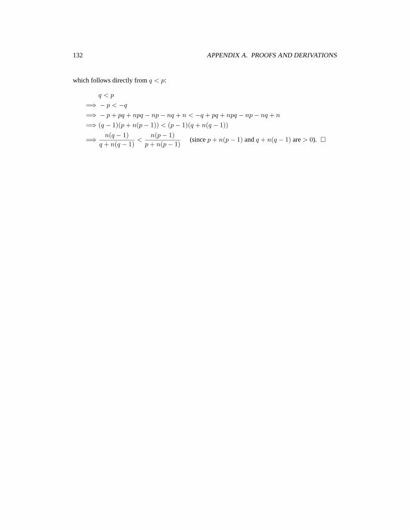
132 APPENDIX A. PROOFS AND DERIVATIONS
which follows directly from q < p:
q < p
=⇒ − p < −q=⇒ − p+ pq + npq − np− nq + n < −q + pq + npq − np− nq + n
=⇒ (q − 1)(p+ n(p− 1)) < (p− 1)(q + n(q − 1))
=⇒ n(q − 1)q + n(q − 1)
<n(p− 1)
p+ n(p− 1)(since p+ n(p− 1) and q + n(q − 1) are > 0). �

Appendix B
Monte Carlo Best-Response Estimation
Here we describe the simulation technique we use to sanity-check equilibria found by our analyticbest-response solver. The approach takes as input an arbitrary payoff function from types and ac-tions of all agents to real-valued payoffs. It also takes an arbitrary strategy function, which is aone-dimensional function from type to action. The strategies and payoffs are represented as arbi-trary Mathematica functions. Additionally, it takes an arbitrary probability distribution from whichtypes are drawn. From these three inputs, it computes an empirical best-response function. Fig-ure 2.2 shows an example of our Monte Carlo method finding the best response to a particularstrategy (see Section 2.4).
At the core of the method for empirically generating best-response strategies is a simulatorthat takes the given payoff function, other agent strategies, other agent type distributions, and aparticular own type and action. The simulator then repeatedly samples from the other agents’ typedistributions, computing for each sampled type the actions according to the known other agentstrategies. The resulting payoff is then computed for the given own type and action by evaluatingthe payoff function. Sample statistics for these payoffs are then recorded and the process is repeatedfor every combination of own type and action, down to a specified granularity. However, certainshortcuts are taken to avoid needless simulation. First, when simulating different actions for agiven type, a confidence bound is continually computed using the sampling statistics for the variousactions sampled so far. Further simulation is limited to the range of actions within the confidencebound (designated in Figure B.1 by the two larger dots at a = 0.25 and a = 1). The confidencebounds are determined by performing mean difference tests on pairs of expected payoff samplestatistics and considering any actions that fail at the 95% level to be within the confidence bound forbest action. It is these confidence bounds that the error bars represent in Figure 2.2. The amount ofsimulation for each type-action pair is dynamically determined based on the confidence intervals forthe expected payoffs. And within the confidence bound of possible actions, the confidence intervalsare compared to prioritize the computation for different actions.
Figure B.1 shows the Monte Carlo best-response method sampling possible actions for a specifictype. It dynamically limits the actions that it samples from by comparing expected payoffs andfinding an interval likely to contain the best action.
133

134 APPENDIX B. MONTE CARLO BEST-RESPONSE ESTIMATION
0 0.25 0.5 0.75 1 1.25 1.5Action
0
0.1
0.2
0.3
0.4
0.5
0.6
ExpectedPayoff
Figure B.1: Empirically estimating the best action for a given type (0) against a given strategy (seeFigure 2.2). After < 20 simulations per action the best action is determined, based on the 95%confidence intervals, to be between 0.25 and 1. The maximum likelihood best action is 0.62 (after100 total samples) and the actual best action is 0.582.

Appendix C
Notes on Equilibria in Symmetric Games
In a symmetric game, every player is identical with respect to the game rules (Definition 1.2). Weinclude here three theorems about the existence of equilibria in symmetric games. (1) A symmetric2-strategy game must have a pure-strategy Nash equilibrium. (2) As a special case of a theoremin Nash’s [1951] seminal paper, any finite symmetric game has a symmetric Nash equilibrium.1
(3) Symmetric infinite games with compact, convex strategy spaces and continuous, quasiconcaveutility functions have symmetric pure-strategy Nash equilibria.
Theorem C.1 A symmetric game with two strategies has an equilibrium in pure strategies.
Proof. Let S = {1, 2} and let [i, n − i] denote the profile with i ∈ {0, . . . , n} players playingstrategy 1 and n − i playing strategy 2. Let ui
s ≡ u(s, [i, n − i]) be the payoff to a player playingstrategy s ∈ S in the profile [i, n− i]. Define the boolean function pe(i) as follows:
pe(i) ≡⎧⎨⎩
u02 ≥ u1
1 if i = 0un
1 ≥ un−12 if i = n
ui1 ≥ ui−1
2 & ui2 ≥ ui+1
1 if i ∈ {1 . . . n− 1}.In words, pe(i) = TRUE when no unilateral deviation from [i, n−i] is beneficial—i.e., when [i, n−i]is a pure-strategy equilibrium.
Assuming the opposite of what we want to prove, pe(i) = FALSE for all i ∈ {0, . . . , n}. Wefirst show by induction on i that ui
2 < ui+11 for all i ∈ {0, . . . , n − 1}. The base case, i = 0,
follows directly from pe(0) = FALSE. For the general case, suppose uk2 < uk+1
1 for some k ∈{0, . . . , n− 2}. Since pe(k+ 1) = FALSE, we have uk+1
1 < uk2 or uk+1
2 < uk+21 . The first disjunct
contradicts the inductive hypothesis, implying uk+12 < uk+2
1 , which concludes the inductive proof.In particular, un−1
2 < un1 . But, pe(n) = FALSE implies un
1 < un−12 , and we have a contradiction.
Therefore pe(i) = TRUE for some i. �
Can we relax the sufficient conditions of Theorem C.1? First, consider symmetric games withmore than two strategies. Rock-Paper-Scissors (Table C.1a) is a counterexample showing that thetheorem no longer holds. It is a three-strategy symmetric game with no pure-strategy equilibrium.This is the case because, of the six pure-strategy profiles (RR, RP, RS, PP, PS, SS), none constitutean equilibrium.
1 We also discuss here Nash’s generalized notion of symmetry in games.
135

136 APPENDIX C. NOTES ON EQUILIBRIA IN SYMMETRIC GAMES
Table C.1: (a) Rock-Paper-Scissors: a 3-strategy symmetric game with no pure-strategy equilibria.(b) Matching Pennies: a 2-strategy asymmetric game with no pure-strategy equilibria. (c) Anti-coordination Game: a symmetric game with no symmetric pure equilibria.
R P SR 0,0 -1,1 1,-1P 1,-1 0,0 -1,1S -1,1 1,-1 0,0
H TH 1,0 0,1T 0,1 1,0
A BA 0,0 1,1B 1,1 0,0
(a) (b) (c)
Next, does the theorem apply to asymmetric two-strategy games? Again, no, as demonstratedby Matching Pennies (Table C.1b). In Matching Pennies, both players simultaneously choose anaction—heads or tails—and player 1 wins if the actions match and player 2 wins otherwise. Again,none of the pure-strategy profiles (HH,TT,HT,TH) constitute an equilibrium.
Finally, can we strengthen the conclusion of Theorem C.1 to guarantee symmetric pure-strategyequilibria? A simple anti-coordination game (Table C.1c) serves as a counterexample. In thisgame, each player receives 1 when the players choose different actions and 0 otherwise. The onlypure-strategy equilibria are the profiles where the players choose different actions, i.e., asymmetricprofiles.
We next consider other sufficient conditions for pure and/or symmetric equilibria in symmetricgames. First we present a lemma establishing properties of the mapping from profiles to best re-sponses. The result is analogous to Lemma 8.AA.1 in Mas-Colell et al. [1995], adapted to the caseof symmetric games.
Lemma C.2 In a symmetric game [n, S, u()] with S nonempty, compact, and convex and withu(si, s1, . . . , sn) continuous in (s1, . . . , sn) and quasi-concave in si, the best response correspon-dence
b(s) ≡ arg maxt∈S
u(t, s)
= {τ : u(τ, s) = maxt∈S
u(t, s)}
is nonempty, convex-valued, and upper hemicontinuous.
Proof. Since u(S, s) is the continuous image of the compact set S, it is compact and has a maximumand so b(s) is nonempty. b(S) is convex because the set of maxima of a quasiconcave function(u(·, s)) on a convex set (S) is convex. To show that b(·) is upper hemicontinuous, show that forany sequence sn → s such that sn ∈ b(sn) for all n, we have s ∈ b(s). To see this, note that for alln, u(sn
i , sn) ≥ u(s′i, sn) for all s′i ∈ S. So by continuity of u(·), we have u(si, s) ≥ u(s′i, s). �
We now show our second main result, that infinite symmetric games with certain properties havesymmetric equilibria in pure strategies. This result corresponds to Proposition 8.D.3 in Mas-Colellet al. [1995] which establishes the existence of (possibly asymmetric) pure strategy equilibria forthe corresponding class of possibly asymmetric games.

137
Theorem C.3 A symmetric game [n, S, u()] with S a nonempty, convex, and compact subset ofsome Euclidean space and u(si, s1, . . . , sn) continuous in (s1, . . . , sn) and quasiconcave in si hasa symmetric pure-strategy equilibrium.
Proof. b(·) is a correspondence from the nonempty, convex, compact set S to itself. By Lemma C.2,b(·) is a nonempty, convex-valued, and upper hemicontinuous correspondence. Thus, by Kakutani’sTheorem2, there exists a fixed point of b(·) which implies that there exists an s ∈ S such thats ∈ b(s) and so all playing s is a symmetric equilibrium. �
Finally, we present Nash’s [1951] result that finite symmetric games have symmetric equilibria.3
This is a special case of his result that every finite game has a “symmetric” equilibrium, whereNash’s definition of a symmetric profile is one invariant under every automorphism of the game.This turns out to be equivalent to defining a symmetric profile as one in which all the symmetricplayers (if any) are playing the same mixed strategy. In the case of a symmetric game, the twonotions of a symmetric profile (invariant under automorphisms vs. simply homogeneous) coincideand we have our result.
Here we present an alternate proof of the result, modeled on Nash’s seminal proof of the exis-tence of (possibly asymmetric) equilibria for general finite games.4
Theorem C.4 A finite symmetric game has a symmetric mixed-strategy equilibrium.
Proof. For each pure strategy s ∈ S, define a continuous function of a mixed strategy σ by
gs(σ) ≡ max(0, u(s, σ)− u(σ, σ)).
In words, gs(σ) is the gain, if any, of unilaterally deviating from the symmetric mixed profile of allplaying σ to playing pure strategy s. Next define
ys(σ) ≡ σs + gs(σ)1 +
∑t∈S gt(σ)
.
The set of functions ys(·)∀s ∈ S defines a mapping from the set of mixed strategies to itself. Wefirst show that the fixed points of y(·) are equilibria. Of all the pure strategies in the support of σ,one, say w, must be worst, implying u(w, σ) ≤ u(σ, σ) which implies that gw(σ) = 0.
Assume y(σ) = σ. Then y must not decrease σw. The numerator is σw so the denominatormust be 1, which implies that for all s ∈ S, gs(σ) = 0 and so all playing σ is an equilibrium.
Conversely, if all playing σ is an equilibrium then all the g’s vanish, making σ a fixed pointunder y(·).
Finally, since y(·) is a continuous mapping of a compact, convex set, it has a fixed point byBrouwer’s Theorem. �
2 For this and other fixed point theorems (namely Brouwer’s, used in Theorem C.4) see, for example, the mathematicalappendix (p952) of Mas-Colell et al. [1995].
3 This result can also be proved as a corollary to Theorem C.3 by viewing a finite game as an infinite game with strategysets being possible mixtures of pure strategies.
4In Nash’s [1950] PhD thesis, he proved this theorem using his contemporary Kakutani’s generalization of Brouwer’sfixed-point theorem to the case of correspondences (point-to-set mappings) but in a subsequent publication [Nash, 1951] hepresented a simplified proof that required only Brouwer’s fixed-point theorem. Theorem C.4 is modeled on the simplifiedproof.

138 APPENDIX C. NOTES ON EQUILIBRIA IN SYMMETRIC GAMES
Since exploitation of symmetry has been known to produce dramatic simplifications of opti-mization problems [Boyd, 1990] it is somewhat surprising that it has not been actively addressed inthe game theory literature. In addition to the methods we have used for game solving and that wediscuss in Section 3.6 (replicator dynamics and function minimization with Amoeba), we believesymmetry may be productively exploited for other algorithms as well. For example, the well-knownLemke-Howson algorithm for 2-player (bimatrix) games lends itself to a simplification if the gameis symmetric and if we restrict our attention to symmetric equilibria: we need only one payoffmatrix, one mixed strategy vector, and one slackness vector, reducing the size of the Linear Com-plementarity Problem by a factor of two. As we discuss in Section 3.6, exploiting symmetry ingames with more than two players can yield enormous computational savings. Finally, as notedin Section 3.9, Bhat and Leyton-Brown [2004] have recently published an algorithm for solving aclass of games which they extend to exploit symmetry.

Appendix D
Strategies for SAA Experiments
This appendix describes in detail the strategies used in our experiments in Chapter 5, in particularthe price prediction strategies. Table D.1 lists all the strategies we consider.
D.1 Price Predicting Strategies
Agents using price prediction strategies generate an initial, pre-auction belief about the final pricesof the goods. For example, the agent can believe that the final prices will all equal zero or they aredistributed normally or uniformly on some interval. The derivation of most beliefs we employ in-volves Monte Carlo sampling. To obtain a belief for a particular distribution of agents’ preferences,we simulate a large number of game instances with agents drawn from the preference distribution.
In most of our reported results we use the uniform and exponential distributions of number ofgoods demanded by the agent. We have also considered agents who demanded a fixed number ofgoods. We refer to such a preference distribution as a fixed distribution. (See Section 5.1 for detailson preference (type) distributions in SAA.)
We consider two families of price predictors (Section 4.5). The point prediction strategy familyhas point beliefs about the final prices that will be realized for each good. The point price predictingstrategy is thus parameterized by its vector of point beliefs. We label such beliefs π(∅). Any pricevector can represent initial beliefs. Point beliefs based on sampling are obtained by averaging acrossfinal prices or demands in the simulated games.
The point prediction family includes a sub-class of strategies with participation-only prediction.The idea behind this strategy is that it ignores its predictions at some stages of decision making(unlike the full point predictor, which always relies on the predicted vector). We describe thisstrategy in Section 5.5.
The distribution prediction strategy family has beliefs about the final price distributions. LetF ≡ F (∅) denote a joint cumulative distribution function over final prices, representing the agent’spre-auction belief. We assume that prices are bounded above by a known constant, V . Thus, Fassociates cumulative probabilities with price vectors in {0, . . . , V }m. For simplicity we use onlythe information contained in the vector of marginal distributions, (F1, . . . , Fm), as if the final pricesare independent across goods.
For technical reasons we require that initial beliefs are such that for each good all prices in{0, . . . , V } have a positive probability of occurring. To ensure that this requirement is satisfied forinitial beliefs obtained from empirical samples, we modify the latter before constructing beliefs. In
139

140 APPENDIX D. STRATEGIES FOR SAA EXPERIMENTS
Strategy Family Family Parameter Examplesand Notation
Straightforward N/A SBbidder, SBSunk-Aware Sunk-awareness SA(k)agent, SA(k) parameter, k k = 0, 0.05, 0.1, . . . 0.95Point Price Beliefs about PP(πZero)Predictors, average final PP(π∞)PP(πx) prices of PP(πECE)
the goods PP(πEDCE)PP(πSB)PP(πSC)
Point Price Beliefs about PPpo(π∞)Predictors average final PPpo(πZero)with participation prices of PPpo(πECE)only, the goods PPpo(πEDCE)PPpo(πx) PPpo(πSB)
PPpo(πSC)Price Beliefs about PP(FZero)Distribution final price PP(FU )Predictors, distributions; PP(FSB)PP(F x) such beliefs are PP(FCE)PP(G(μ(x), σ(y))) labeled by x PP(G(μ(CE), σ(CE)))
or a pair (μ,σ) PP(G(μ(SB), σ(SB)))PP(F (πx)) PP(F (πECE))
PP(F (πEDCE))PP(F (πSB))PP(F (πSC))
Table D.1: Reference table. The strategy families we have studied are listed in column 1 and theirparameters are in column 2. Column 3 lists strategies we have employed in many of our restrictedgames.

D.1. PRICE PREDICTING STRATEGIES 141
particular, we add to the empirically obtained sample of prices a sample of (V + 1) prices from 0to V . Suppose the empirical sample consists of N games. The probability that the good will havefinal price p ∈ {0, . . . , V } is then
Pr(p) =Np + 1
N + (V + 1), (D.1)
where Np is the number of times the final price equaled p in the original sample. If N is highrelative to V, the effect of adding an artificial sample to the empirical one is negligible. In therestricted games we studied V = 50 and N ≥ 340,000.
In the following sections we describe some examples of beliefs. We denote a specific point priceprediction strategy by PP(πx), where x labels particular initial point beliefs, π(∅). We denote thestrategy of bidding based on a particular distribution predictor by PP(Fx), where x labels variousinitial beliefs about final price distributions, F (∅). If the initial beliefs x are based on Monte Carlosampling, we write xu and xe to distinguish between beliefs obtained using draws from uniformand exponential preference distributions.1
Zero Beliefs
To construct zero beliefs for the distribution predictor, we assume that we have a sample of n = 106
zero final prices. After we add another artificial sample of (V +1) = 51 prices (see Equation D.1),the probability that the final price of a good will be zero becomes 1,000,000/1,000,051 = 0.99995.The probability that the final price of this good will equal p ∈ [1, V ] becomes 1/1,000,051 < 10−6.Note, however, that as soon as the ask price exceeds zero, the distribution predictor reconditions itsbeliefs based on that information. So once all the ask prices are above zero it bids identically to adistribution predictor having a uniform distribution for final prices.
For the point price predictor, zero beliefs are simply a vector of zeros. The point price predictorwith zero beliefs is equivalent to SB. We denote the distribution predictors using zero beliefs byPP(FZero). A point predictor with zero beliefs is PP(0), or, for consistency, PP(πZero), or ofcourse simply SB.
Infinite Point Beliefs
Infinite point beliefs are defined only for the point price predictor. We label such a predictorPP(π∞). We define this strategy so that it reverts to SB if the agent has single-unit preference.Since there is no exposure problem, such an agent will bid if and only if it has a positive value forexactly one of the goods (despite the expectation that the price will be infinite). Thus, this strategyrepresents the extreme of conservative bidding, never risking exposure. The performance of thisstrategy provides a useful performance benchmark for price predicting strategies.
Uniform Distribution Beliefs
The uniform distribution beliefs are defined only for the distribution predictor, which we denotePP(FU ). According to the uniform beliefs, the probability that the final price of a good will equalp ∈ [0, V ] is 1/51 = 0.0196.
1We suppress this subscript when it is clear from context (see Section D.3).

142 APPENDIX D. STRATEGIES FOR SAA EXPERIMENTS
Baseline Beliefs
Baseline beliefs are based on the final prices in a sample of games in which all players use theSB strategy. The baseline point beliefs are a vector of average final prices of the goods available.The baseline distribution beliefs are a vector of marginal price distributions computed according toEquation D.1. Our sample size is N = 106 games, and the upper bound on prices is V = 50 for allgoods.
We denote the point predictors with SB beliefs derived using samples from the uniform andexponential distributions by PP(πSBu) and PP(πSBe) respectively. Similarly, the distributionpredictors with SB beliefs are labeled PP(FSBu) and PP(FSBe).
Walrasian Equilibrium Beliefs
Suppose that the final prices form a Walrasian price equilibrium (PE) in the SAA game. This isguaranteed, for example, when SB agents all demand only single goods, but is not true in general.However, in our experience, the final prices are generally not too far from PE. Therefore, wecalculate the Walrasian equilibrium for an SAA environment and use the resulting prices to createinitial beliefs.
Let SE be an SAA environment. To find the vector of Walrasian equilibrium price distributionsfor SE, FPE , we randomly generate many (N = 25000) game instances with agents drawn fromthe preference distribution of SE, and use tatonnement to solve for the equilibrium prices in each.(See Chapter 4 for details.) The PE distribution beliefs are computed based on the sample of theequilibrium prices according to Equation D.1. We label the PE distribution predictor as PP(FPEu)if the preference distribution of the sample is uniform, and as PP(FPEe) if it is exponential.
We calculate the expected price equilibrium beliefs, πEPE , by averaging across the prices in thesample. We calculate the expected demand price equilibrium beliefs, πEDPE , by calculating theexpected demand function for each of the game instances, and then solving for the Walrasian equi-librium based on the average demands. We label the corresponding bid strategies as PP(πEPEu)and PP(πEDPEu) if the preference distribution of the sample is uniform, and as PP(πEPEe) andPP(πEDPEe) if it is exponential.2 We describe the Walrasian prediction approach in greater detailin Chapter 4.
Self-Confirming Prices
The self-confirming (SC) distribution beliefs are what we call self-confirming marginal price dis-tributions (Section 4.6). Let SE be an SAA environment. The prediction F = (F1, . . . , Fm)is a vector of self-confirming marginal price distributions for SE iff for all i, Fi is the marginaldistribution of prices for good i resulting when all agents play bidding strategy PP(F ) in SE.
The SC point beliefs are what we call self-confirming point predictions, which are defined as avector of point predictions (π) that on average are correct, if all agents use point price prediction.Note that the mean of an SC distribution may be different from SC point predictions for the sameenvironment.
The general idea behind the derivation algorithms of both types of self-confirming predictions isas follows. Given an SAA environment, we derive self-confirming predictions through an iterative
2The prices to which tatonnement converges are sensitive to the choice of initial prices and other parameters of thealgorithm. In Section D.2 we list all the price vectors we obtained for the 5×5 uniform environment. We have not derivedPE beliefs for alternative environments.

D.2. 53-STRATEGY GAME FOR 5×5 UNIFORM ENVIRONMENT 143
simulation process. Starting from an arbitrary prediction, we run many instances (N ) of an SAAenvironment (sampling from the given preference distributions) with all agents playing the samepredicting strategy (either point prediction or distribution prediction). We record the resulting pricesfrom each instance, and create new beliefs for the predictors. The new point beliefs are a vector ofaverage final prices from the first iteration. The new distribution beliefs are the sample distribution.We repeat the process using the new beliefs for each new iteration. If it ever reaches an approximatefixed point, then we have statistically identified approximate self-confirming predictions for thisenvironment. We describe further details of SC point prediction in Section 4.6 and SC distributionprediction there and in other work [Osepayshvili et al., 2005].
For the environments we investigate, we can find both SC point predictions and distributions.In our experiments, N = 500,000 for SC point predictions and N = 106 for SC distributions; theinitial beliefs used in the first iteration are zero beliefs (Section D.1), although our results do notappear sensitive to this.
Gaussian Distribution Beliefs
The Gaussian distribution beliefs are defined only for the distribution predictor. Suppose we knowthe expected prices μ and the standard deviations σ for all the goods. Then we can approximatethe final price distribution of good i with a Gaussian centered on μi with the restriction that pricesp ∈ [0, V ]. To implement Gaussian beliefs we draw a random sample of size N = 1000000 fromN(μi, σi) for each good i and discard prices outside [0, V ].3 Then we compute the final priceprobabilities according to Equation D.1. We denote distribution predictors with such beliefs byG(μ,σ), where μ and σ label the expected prices and standard deviations. For example, strategyPP(G(μ(PEu), σ(PEu))) has Gaussian beliefs created using the means and standard deviations ofthe distribution vector FPEu ; agent PP(G(πEDPEu , σ(PEu))) has Gaussian beliefs created usingπEDPEu as the means vector and the standard deviations of the distribution vector FPEu .
Degenerate Distribution Beliefs
The degenerate distribution beliefs are defined only for the distribution predictor. They are degen-erate in the sense that according to such beliefs each good has a deterministic final price. Let π bea vector of prices. For every good i, assign probability 1 to the ith element of π and probability 0to all other prices in [0, V ]. We denote the distribution predictor with such beliefs by PP(F (π)).If we round the vector π before generating the distributions, we mark the vector by a prime in thestrategy name: PP(F (π
′)). For example, PP(F (πSBu)) has beliefs that the final prices will equal
πSBu with probability 1; PP(F (πEPE′u)) has beliefs that the final prices will equal the rounded
elements of πEPEu with probability 1. The former beliefs match better the information that thecorresponding point predictor has. The latter beliefs are justified by the fact that prices are integersin our model.
D.2 53-Strategy Game For 5×5 Uniform Environment
We constructed 53 strategies for the 5×5 uniform environment (Section 5.7). In Table D.2 we listall the strategies, relevant sections of this appendix and all our publications in which the strategies
3One drawback of this approach is that truncating the tails shifts the means of the distribution.

144 APPENDIX D. STRATEGIES FOR SAA EXPERIMENTS
Strategy Family # Strategy Notation
N/A 1 SBSunk-Aware 20 SA(k)
k = 0, 0.05, 0.1, . . . 0.95Point Price 13 PP(π∞),Predictors PP(πSBu), PPpo(πSBu),
PP(πEPEu), PP(πEPE∗u), PP(πEPE∗∗
u ),PP(πEPEe), PP(πEPE∗
e ),PP(πEDPEu), PP(πEDPE∗
u),PP(πEDPEe), PP(πEDPE∗
e ),PP(πSCu)
Price 19 PP(FZero),PP(FU )Distribution PP(FSBu),PP(FSCu),Predictors PP(FPEu),
PP(G(μ(PEu), σ(PEu))),PP(G(μ(SBu), σ(SBu))),PP(G(πEDPEu , σ(PEu))),PP(G(πEDPEu , σ(SBu))),PP(G(πSCu , σ(PEu))),PP(G(πSCu , σ(SBu))),PP(F (πEPEu)), PP(F (πEPE′
u)),PP(F (πEDPEu)), PP(F (πEDPE′
u)),PP(F (πSBu)), PP(F (πSB′
u))PP(F (πSCu)), PP(F (πSC′
u))
Table D.2: 53 strategies for the largest 5×5 uniform environment game. The strategies are listedin column 3, and their strategy families are given in column 1. The po subscript refers to partic-ipation only prediction. Different point beliefs created by the same (non-deterministic) algorithmare marked by asterisks. Column 2 gives the total number of strategies from a particular familyrepresented in the 53-strategy game.
were mentioned. Table D.3 presents all initial point beliefs for the price predicting strategies wederived for the 5×5 uniform environment, as well as relevant sections of this appendix.
D.3 Strategies For Alternative Environments
Table D.4 describes the pool of 27 strategies that we searched for a profitable deviation from playingPP(FSC) when all the other agents play PP(FSC). Table D.5 describes 7-strategy games (7-cliques) for each of the alternative environments we consider (Section 5.7). Some of the strategiesare price predictors whose initial beliefs are derived using Monte Carlo sampling. Such beliefsare therefore parameterized by the underlying preference distribution. However, we suppress thepreference distribution labels in the tables, because we derived these beliefs only for the environmentin which the corresponding predicting strategy was used, and therefore there is no ambiguity abouthow the beliefs were derived.

D.3. STRATEGIES FOR ALTERNATIVE ENVIRONMENTS 145
Beliefs/Good Initial Point Beliefs Appendix Sectionπ∞ 1000 1000 1000 1000 1000 D.1πSBu 14.8 10.7 7.6 4.6 1.9 D.1πSCu 13.0 8.7 5.4 3.0 1.2 D.1πEPEu 16.6 10.8 6.5 3.1 0.7 D.1πEPE∗
u 16.5 10.7 6.4 3.1 0.8 D.1πEPE∗∗
u 26.0 14.2 6.9 2.5 0.3 D.1πEPEe 6.0 4.1 1.8 0.6 0.1 D.1πEPE∗
e 30.5 11.9 6.0 2.7 0.4 D.1πEDPEu 20.0 12.0 8.0 2.0 0.0 D.1πEDPE∗
u 20.8 11.4 8.2 1.8 0.0 D.1πEDPEe 25.0 10.0 5.1 0.9 0.0 D.1πEDPE∗
e 24.5 10.5 5.5 1.5 0.0 D.1
Table D.3: Initial beliefs (rounded to one decimal place) for the 5×5 uniform environment. Thenotation for the beliefs is presented in column 1. The vectors of point beliefs for the five goodsare presented in column 2. The monotonicity of the prices is due to the specifics of the preferencedistribution (Section 5.1). The subsections of Section D.1 that are most relevant to a particular beliefare presented in column 3.
Strategy Family # Strategy Notation
N/A 1 SBSunk- 20 SA(k)Aware k = 0, 0.05, 0.1, . . . 0.95Point Price 3 PP(π∞), PP(πSB), PP(πSC)PredictorsPrice Distribution 3 PP(FU ), PP(FSB), PP(FSC)Predictors
Table D.4: Pool of 27 deviators for alternative environments. The strategies are listed in column 3,and their strategy families are given in column 1. Column 2 gives then total number of strategiesfrom a particular family represented in the 27-strategy pool.

146 APPENDIX D. STRATEGIES FOR SAA EXPERIMENTS
Environment StrategiesE(3, 3) PP(FSC), PP(FSB), SA(0.6), SA(0.7), SA(0.75), SA(0.8), SA(0.85)E(3, 5) PP(FSC), PP(FSB), PP(FU ), PP(πSC), PP(πSB), PP(π∞), SA(0.85)E(3, 8) PP(FSC), PP(FSB), PP(FU ), PP(πSC), PP(πSB), PP(π∞), SA(0.85)E(5, 3) PP(FSC), PP(FSB), PP(FU ), PP(πSC), PP(πSB), PP(π∞), SBE(5, 5) PP(FSC), PP(FSB), PP(FU ), PP(πSC), PP(πSB), PP(π∞), SA(0.35)E(5, 8) PP(FSC), PP(FSB), PP(FU ), PP(πSC), PP(πSB), PP(π∞), SA(0.35)E(7, 3) PP(FSC), PP(FSB), SA(0.55), SA(0.65), SA(0.7), SA(0.75), SA(0.8)E(7, 6) PP(FSC), PP(FSB), PP(FU ), PP(πSC), PP(πSB), PP(π∞), SBU(3, 3) PP(FSC), PP(FSB), SA(0.65), SA(0.7), SA(0.75), SA(0.8), SA(0.85)U(3, 5) PP(FSC), PP(FSB), PP(πSC), PP(πSB), SA(0.7), SA(0.75), SA(0.85)U(3, 8) PP(FSC), PP(FSB), PP(FU ), PP(πSC), PP(πSB), PP(π∞), SA(0.9)U(5, 3) PP(FSC), PP(FSB), SA(0.6), SA(0.65), SA(0.7), SA(0.75), SA(0.8)U(5, 8) PP(FSC), PP(FSB), PP(FU ), PP(πSC), PP(πSB), PP(π∞), SA(0.9)U(7, 3) PP(FSC), PP(FSB), SA(0.55), SA(0.65), SA(0.7), SA(0.75), SA(0.8)U(7, 6) PP(FSC), PP(FSB), PP(πSC), PP(πSB), SA(0.75), SA(0.8), SA(0.9)U(7, 8) PP(FSC), PP(FSB), PP(FU ), PP(πSC), PP(πSB), PP(π∞), SB
Table D.5: 7-strategy games for alternative environments. E(m,n) and U(m,n) refer to variousSAAλ∼U and SAAλ∼E environments.

Bibliography
Olivier Armantier, Jean-Pierre Florens, and Jean-Francois Richard. Empirical game-theoretic mod-els: Constrained equilibrium and simulations. Technical report, State University of New York atStonybrook, 2000.
Olivier Armantier, Jean-Pierre Florens, and Jean-Francois Richard. Approximation of BayesianNash equilibria. Games and Economic Behavior, to appear.
Kenneth J. Arrow and Frank H. Hahn. General Competitive Analysis. Holden-Day, San Francisco,1971.
W. Brian Arthur, John H. Holland, Blake LeBaron, Richard Palmer, and Paul Tayler. Asset pric-ing under endogenous expectations in an artificial stock market. In W. Brian Arthur, Steven N.Durlauf, and David A. Lane, editors, The Economy as an Evolving Complex System II. Addison-Wesley, 1997.
Susan Athey. Single crossing properties and the existence of pure strategy equilibria in games ofincomplete information. Econometrica, 69(4):861–890, 2001.
Robert J. Aumann and Sergiu Hart. Handbook of Game Theory, volume 1. North-Holland, 1992.
Thomas Becker and Volker Weispfenning. Grobner Bases: A Computational Approach to Commu-tative Algebra. Springer-Verlag, New York, 1993.
Dimitri P. Bertsekas. Auction algorithms for network flow problems: A tutorial introduction. Com-putational Optimization and Applications, 1:7–66, 1992.
Navin A. R. Bhat and Kevin Leyton-Brown. Computing Nash equilibria of action-graph games. InTwentieth Conference on Uncertainty in Artificial Intelligence, pages 35–42, Banff, 2004.
Sushil Bikhchandani and John W. Mamer. Competitive equilibrium in an exchange economy withindivisibilities. Journal of Economic Theory, 74:385–413, 1997.
Ben Blum, Christian R. Shelton, and Daphne Koller. A continuation method for Nash equilibria instructured games. In Eighteenth International Joint Conference on Artificial Intelligence, pages757–764, Acapulco, 2003.
Prosenjit Bose, Anil Maheshwari, and Pat Morin. Fast approximations for sums of distances, clus-tering, and the Fermat-Weber problem. Computational Geometry: Theory and Applications,24(3):135–146, 2003.
147

148 BIBLIOGRAPHY
Justin Boyan and Amy Greenwald. Bid determination in simultaneous auctions: An agent architec-ture. In Third ACM Conference on Electronic Commerce, pages 210–212, Tampa, FL, 2001.
John H. Boyd. Symmetries, dynamic equilibria, and the value function. In R. Ramachandran andR. Sato, editors, Conservation Laws and Symmetry: Applications to Economics and Finance.Kluwer, Boston, 1990.
Felix Brandt and Gerhard Weiß. Antisocial agents and Vickrey auctions. In Eighth InternationalWorkshop on Agent Theories, Architectures, and Languages, volume 2333 of Lecture Notes inComputer Science, pages 335–347, Seattle, 2001. Springer.
Felix Brandt, Tuomas Sandholm, and Yoav Shoham. Spiteful bidding in sealed-bid auctions. Tech-nical report, Stanford University, 2005.
George W. Brown. Iterative solution of games by fictitious play. In T. C. Koopmans, editor, ActivityAnalysis of Production and Allocation, pages 374–376. Wiley, New York, 1951.
Bruno Buchberger. Grobner bases: An algorithmic method in polynomial ideal theory. In Nirmal K.Bose, editor, Multidimensional Systems Theory. Van Nostrand Reinhold, New York, 1982.
Andrew Byde. Applying evolutionary game theory to auction mechanism design. Technical ReportHPL-2002-321, HP Laboratories Bristol, 2002.
Kaylan Chatterjee and W. F. Samuelson. Bargaining under incomplete information. OperationsResearch, 31:835–851, 1983.
Shih-Fen Cheng, Daniel M. Reeves, Yevgeniy Vorobeychik, and Michael P. Wellman. Notes onequilibria in symmetric games. In AAMAS-04 Workshop on Game Theory and Decision Theory,New York, 2004.
Shih-Fen Cheng, Evan Leung, Kevin M. Lochner, Kevin O’Malley, Daniel M. Reeves, L. JulianSchvartzman, and Michael P. Wellman. Walverine: A Walrasian trading agent. Decision SupportSystems, 39:169–184, 2005.
Dave Cliff. Evolving parameter sets for adaptive trading agents in continuous double-auction mar-kets. In Agents-98 Workshop on Artificial Societies and Computational Markets, pages 38–47,Minneapolis, MN, 1998.
Dave Cliff. Explorations in evolutionary design of online auction market mechanisms. ElectronicCommerce Research and Applications, 2:162–175, 2003.
Augustin Cournot. Researches into the mathematical principles of the theory of wealth, 1838.English Edition, ed. N. Bacon (Macmillan, 1897).
Peter Cramton, Yoav Shoham, and Richard Steinberg, editors. Combinatorial Auctions. MIT Press,2005.
Peter Cramton. Money out of thin air: The nationwide narrowband PCS auction. Journal of Eco-nomics and Management Strategy, 4:267–343, 1995.
Peter Cramton. Simultaneous ascending auctions. In Peter Cramton, Yoav Shoham, and RichardSteinberg, editors, Combinatorial Auctions. MIT Press, 2005.

149
Janosz A. Csirik, Michael L. Littman, Satinder Singh, and Peter Stone. FAucS: An FCC spectrumauction simulator for autonomous bidding agents. In Second International Workshop on Elec-tronic Commerce, volume 2232 of Lecture Notes in Computer Science, pages 139–151. Springer-Verlag, 2001.
Richard Dawkins. The Selfish Gene. Oxford University Press, 1976.
Sven de Vries and Rakesh Vohra. Combinatorial auctions: A survey. INFORMS Journal on Com-puting, 15:284–309, 2003.
Gerard Debreu. A social equilibrium existence theorem. Proceedings of the National Academy ofSciences, 38:886–893, 1952.
Ronald Fagin, Joseph Y. Halpern, Yoram Moses, and Moshe Y. Vardi. Reasoning about Knowledge.MIT Press, 1995.
Daniel Friedman and John Rust, editors. The Double Auction Market. Addison-Wesley, 1993.
Daniel Friedman. Evolutionary games in economics. Econometrica, 59:637–666, 1991.
Clemens Fritschi and Klaus Dorer. Agent-oriented software engineering for successful tac partici-pation. In First International Joint Conference on Autonomous Agents and Multi-Agent Systems,Bologna, Italy, 2002.
Drew Fudenberg and David K. Levine. The Theory of Learning in Games. MIT Press, 1998.
Drew Fudenberg and Jean Tirole. Game Theory. MIT Press, 1991.
M. Galassi, J. Davies, J. Theiler, B. Gough, G. Jungman, M. Booth, and F. Rossi. GNU ScientificLibrary Reference Manual (2nd Ed.). ISBN 0954161734, 2002. http://www.gnu.org/software/gsl/.
Herbert Gintis. Game Theory Evolving. Princeton University Press, 2000.
Michael B. Gordy. Computationally convenient distributional assumptions for common-value auc-tions. Computational Economics, 12:61–78, 1998.
Srihari Govindan and Robert Wilson. Structure theorems for game trees. Proceedings of the Na-tional Academy of Sciences, 99(13):9077–9080, 2002.
Srihari Govindan and Robert Wilson. A global Newton method to compute Nash equilibria. Journalof Economic Theory, 110:65–86, 2003.
Amy Greenwald and Justin Boyan. Bidding under uncertainty: Theory and experiments. In Twen-tieth Conference on Uncertainty in Artificial Intelligence, pages 209–216, Banff, 2004.
Amy Greenwald and Peter Stone. The first international trading agent competition: Autonomousbidding agents. IEEE Internet Computing, 5(2):52–60, 2001.
John Harsanyi. Games of incomplete information played by Bayesian players. Management Sci-ence, 14:159–182, 320–334, 486–502, 1967.

150 BIBLIOGRAPHY
Minghua He and Nicholas R. Jennings. SouthamptonTAC: Designing a successful trading agent. InFifteenth European Conference on Artificial Intelligence, pages 8–12, Lyon, 2002.
Minghua He and Nicholas R. Jennings. SouthamptonTAC: An adaptive autonomous trading agent.ACM Transactions on Internet Technology, 3:218–235, 2003.
Shlomit Hon-Snir, Dov Monderer, and Aner Sela. A learning approach to auctions. Journal ofEconomic Theory, 82:65–88, 1998.
John H. Kagel and Dan Levin. Independent private value auctions: Bidder behavior in first-, second-, and third-price auctions with varying numbers of bidders. Economic Journal, 103(419):868–878, 1993.
Michael Kearns, Michael L. Littman, and Satinder Singh. Graphical models for game theory. InSeventeenth Conference on Uncertainty in Artificial Intelligence, pages 253–260, Seattle, 2001.
Alexander S. Kelso and Vincent P. Crawford. Job matching, coalition formation, and gross substi-tutes. Econometrica, 50:1483–1504, 1982.
Jeffrey O. Kephart and Amy R. Greenwald. Shopbot economics. Autonomous Agents and Multia-gent Systems, 5:255–287, 2002.
Jeffrey O. Kephart, James E. Hanson, and Jakka Sairamesh. Price and niche wars in a free-marketeconomy of software agents. Artificial Life, 4:1–23, 1998.
Daphne Koller and Avi Pfeffer. Representations and solutions for game-theoretic problems. Artifi-cial Intelligence, 94(1–2):167–215, 1997.
Daphne Koller, Nimrod Megiddo, and Bernhard von Stengel. Efficient computation of equilibriafor extensive two-person games. Games and Economic Behavior, 14:247–259, 1996.
David M. Kreps. Game Theory and Economic Modelling. Oxford University Press, 1990.
Vijay Krishna and John Morgan. An analysis of the war of attrition and the all-pay auction. Journalof Economic Theory, 72:343–362, 1997.
Vijay Krishna. Auction Theory. Academic Press, 2002.
Pierfrancesco La Mura. Game networks. In Sixteenth Conference on Uncertainty in ArtificialIntelligence, pages 335–342, Stanford, 2000.
Blake LeBaron. Agent-based computational finance: Suggested readings and early research. Jour-nal of Economic Dynamics and Control, 24:679–702, 2000.
Pierre L’Ecuyer. Efficiency improvement and variance reduction. In Winter Simulation Conference,pages 122–132, 1994.
Wolfgang Leininger, Peter Linhart, and Roy Radner. Equilibria of the sealed-bid mechanism forbargaining with incomplete information. Journal of Economic Theory, 48:63–106, 1989.
Carlton E. Lemke and J. T. Howson, Jr. Equilibrium points of bimatrix games. Journal of theSociety for Industrial and Applied Mathematics, 12(2):413–423, 1964.

151
Kevin Leyton-Brown and Moshe Tennenholtz. Local-effect games. In Eighteenth InternationalJoint Conference on Artificial Intelligence, pages 772–777, 2003.
Kevin Leyton-Brown, Mark Pearson, and Yoav Shoham. Towards a universal test suite for combi-natorial auction algorithms. In Second ACM Conference on Electronic Commerce, pages 66–76,2000.
Richard J. Lipton, Evangelos Markakis, and Aranyak Mehta. Playing large games using simplestrategies. In Fourth ACM Conference on Electronic Commerce, pages 36–41, San Diego, 2003.
Jeffrey K. MacKie-Mason and Michael P. Wellman. Automated markets and trading agents. InHandbook of Agent-Based Computational Economics. Elsevier, 2005.
Jeffrey K. MacKie-Mason, Anna Osepayshvili, Daniel M. Reeves, and Michael P. Wellman. Priceprediction strategies for market-based scheduling. In Fourteenth International Conference onAutomated Planning and Scheduling, pages 244–252, Whistler, BC, 2004.
Andreu Mas-Colell, Michael D. Whinston, and Jerry R. Green. Microeconomic Theory. OxfordUniversity Press, New York, 1995.
R. Preston McAfee and John McMillan. Auctions and bidding. Journal of Economic Literature,25:699–738, 1987.
R. Preston McAfee and John McMillan. Analyzing the airwaves auction. Journal of EconomicPerspectives, 10(1):159–175, 1996.
Richard D. McKelvey and Andrew McLennan. Computation of equilibria in finite games. In Hand-book of Computational Economics, volume 1. Elsevier Science, 1996.
Richard D. McKelvey, Andrew McLennan, and Theodore Turocy. Gambit game theory analysissoftware and tools, 1992. http://econweb.tamu.edu/gambit.
Flavio M. Menezes, Paulo K. Monteiro, and Akram Temimi. Private provision of discrete publicgoods with incomplete information. Journal of Mathematical Economics, 35(4):493–514, July2001.
Paul R. Milgrom and John Roberts. Adaptive and sophisticated learning in normal form games.Games and Economic Behavior, 3:82–100, 1991.
Paul R. Milgrom and Robert J. Weber. A theory of auctions and competitive bidding. Econometrica,50(5):1089–1122, 1982.
Paul R. Milgrom and Robert J. Weber. Distributional strategies for games with incomplete informa-tion. Mathematics of Operations Research, 10:619–632, 1985.
Paul Milgrom. Putting auction theory to work: The simultaneous ascending auction. Journal ofPolitical Economy, 108:245–272, 2000.
John Morgan, Ken Steiglitz, and George Reis. The spite motive and equilibrium behavior in auc-tions. Contributions to Economic Analysis and Policy, 2(1), 2003.
John Nash. Non-cooperative games. PhD thesis, Princeton University, Department of Mathematics,1950.

152 BIBLIOGRAPHY
John Nash. Non-cooperative games. Annals of Mathematics, 2(54):286–295, 1951.
John Nash. Two-person cooperative games. Econometrica, 21:128–140, 1953.
John A. Nelder and Roger Mead. A simplex method for function minimization. Computer Journal,7:308–313, 1965.
James Nicolaisen, Valentin Petrov, and Leigh Tesfatsion. Market power and efficiency in a com-putational electricity market with discriminatory double-auction pricing. IEEE Transactions onEvolutionary Computation, 5:504–523, 2001.
Eugene Nudelman, Jennifer Wortman, Yoav Shoham, and Kevin Leyton-Brown. Run the GAMUT:A comprehensive approach to evaluating game-theoretic algorithms. In Third International JointConference on Autonomous Agents and Multi-Agent Systems, pages 880–887, 2004.
Anna Osepayshvili, Michael P. Wellman, Daniel M. Reeves, and Jeffrey K. MacKie-Mason. Self-confirming price prediction for bidding in simultaneous ascending auctions. In Twenty-first Con-ference on Uncertainty in Artificial Intelligence, pages 441–449, July 2005.
Michael Peters and Sergei Severinov. Internet auctions with many traders. Technical report, Uni-versity of Toronto, 2001.
Steve Phelps, Simon Parsons, Peter McBurney, and Elizabeth Sklar. Co-evolution of auction mecha-nisms and trading strategies: Towards a novel approach to microeconomic design. In GECCO-02Workshop on Evolutionary Computation in Multi-Agent Systems, pages 65–72, 2002.
Ryan Porter, Eugene Nudelman, and Yoav Shoham. Simple search methods for finding a Nashequilibrium. In Nineteenth National Conference on Artificial Intelligence, pages 664–669, SanJose, CA, 2004.
William H. Press, Saul A. Teukolsky, William T. Vetterling, and Brian P. Flannery. NumericalRecipes in C. Cambridge University Press, second edition, 1992.
Tony Curzon Price. Using co-evolutionary programming to simulate strategic behaviour in markets.Journal of Evolutionary Economics, 7:219–254, 1997.
Daniel M. Reeves and Michael P. Wellman. Computing best response strategies in infinite games ofincomplete information. In Twentieth Conference on Uncertainty in Artificial Intelligence, pages470–478, Banff, 2004.
Daniel M. Reeves, Michael P. Wellman, Jeffrey K. MacKie-Mason, and Anna Osepayshvili. Ex-ploring bidding strategies for market-based scheduling. Decision Support Systems, 39(1):67–85,March 2005.
John A. Rice. Mathematical Statistics and Data Analysis. Duxbury Press, California, 1995.
Julia Bowman Robinson. An iterative method of solving a game. Annals of Mathematics, 54:296–301, 1951.
Jeffrey S. Rosenschein and Gilad Zlotkin. Rules of Encounter: Designing Conventions for Auto-mated Negotiation among Computers. MIT Press, 1994.

153
Sheldon M. Ross. Simulation (3rd Ed.). Academic Press, 2001.
John Rust, John Miller, and Richard Palmer. Behavior of trading automata in a computerized doubleauction market. In Friedman and Rust [1993], pages 155–198.
Mark A. Satterthwaite and Steven R. Williams. Bilateral trade with the sealed bid k-double auction:Existence and efficiency. Journal of Economic Theory, 48:107–133, 1989.
Mark A. Satterthwaite and Steven R. Williams. The Bayesian theory of the k-double auction. InFriedman and Rust [1993], pages 99–123.
Peter Schuster and Karl Sigmund. Replicator dynamics. Journal of Theoretical Biology, 100:533–538, 1983.
Reinhard Selten and Joachim Buchta. Experimental sealed bid first price auctions with directlyobserved bid functions. Technical Report Discussion Paper B-270, University of Bonn, 1994.
Claude E. Shannon. Programming a computer for playing chess. Philosophical Magazine, 41:256–275, 1950.
Lloyd S. Shapley. Some topics in two-person games. In M. Dresher, L. S. Shapley, and A. W.Tucker, editors, Advances in Game Theory, volume 5 of Annals of Mathematical Studies, pages1–28. 1964.
Satinder Singh, Vishal Soni, and Michael P. Wellman. Computing approximate Bayes-Nash equilib-ria in tree-games of incomplete information. In Fifth ACM Conference on Electronic Commerce,pages 81–90, New York, 2004.
Peter Stone and Amy Greenwald. The first international trading agent competition: Autonomousbidding agents. Journal of Electronic Commerce Research, 5:229–265, 2005.
Peter Stone, Michael L. Littman, Satinder Singh, and Michael Kearns. ATTac-2000: An adaptiveautonomous bidding agent. Journal of Artificial Intelligence Research, 15:189–206, 2001.
Peter Stone, Robert E. Schapire, Janosz A. Csirik, Michael L. Littman, and David McAllester.ATTac-2001: A learning, autonomous bidding agent. In Agent-Mediated Electronic CommerceIV, volume 2153 of Lecture Notes in Computer Science. Springer-Verlag, 2002.
Peter Stone, Robert E. Schapire, Michael L. Littman, Janos A. Csirik, and David McAllester.Decision-theoretic bidding based on learned density models in simultaneous, interacting auc-tions. Journal of Artificial Intelligence Research, 19:209–242, 2003.
Peter Stone. Multiagent competitions and research: Lessons from RoboCup and TAC. In SixthRoboCup International Symposium, Fukuoka, Japan, 2002.
Peter D. Taylor and Leo B. Jonker. Evolutionary stable strategies and game dynamics. MathematicalBiosciences, 40:145–156, 1978.
Theodore L. Turocy. Computation and Robustness in Sealed-bid Auctions. PhD thesis, Northwest-ern University, 2001.

154 BIBLIOGRAPHY
Stanislav Uryasev and Reuven Y. Rubinstein. On relaxation algorithms in computation of non-cooperative equilibria. In IEEE Transactions on Automatic Control (Technical Notes), volume 39,1994.
Eric van Damme. Refinements of the Nash equilibrium concept. In Lecture Notes in Economicsand Mathematical Systems. Springer, Berlin and New York, 1983.
Ioannis A. Vetsikas and Bart Selman. A principled study of the design tradeoffs for autonomoustrading agents. In Second International Joint Conference on Autonomous Agents and Multi-AgentSystems, pages 473–480, Melbourne, 2003.
William Vickrey. Counterspeculation, auctions, and competitive sealed tenders. Journal of Finance,16:8–37, 1961.
John von Neumann and Oskar Morgenstern. Theory of Games and Economic Behavior. PrincetonUniversity Press, 1947.
Leon Walras. Elements of pure economics, 1874. English translation by William Jaffe, publishedby Allen and Unwin, 1954.
William E. Walsh, Michael P. Wellman, and Fredrik Ygge. Combinatorial auctions for supply chainformation. In Second ACM Conference on Electronic Commerce, pages 260–269, 2000.
William E. Walsh, Rajarshi Das, Gerald Tesauro, and Jeffrey O. Kephart. Analyzing complexstrategic interactions in multi-agent systems. In AAAI-02 Workshop on Game-Theoretic andDecision-Theoretic Agents, Edmonton, 2002.
William E. Walsh, David C. Parkes, and Rajarshi Das. Choosing samples to compute heuristic-strategy Nash equilibrium. In AAMAS-03 Workshop on Agent-Mediated Electronic Commerce V,Melbourne, 2003.
William E. Walsh. Market Protocols for Decentralized Supply Chain Formation. PhD thesis, Uni-versity of Michigan, 2001.
Robert J. Weber. Making more from less: Strategic demand reduction in the FCC spectrum auctions.Journal of Economics and Management Strategy, 6:529–548, 1997.
Jorgen W. Weibull. Evolutionary Game Theory. MIT Press, 1995.
Michael P. Wellman, William E. Walsh, Peter R. Wurman, and Jeffrey K. MacKie-Mason. Auctionprotocols for decentralized scheduling. Games and Economic Behavior, 35:271–303, 2001.
Michael P. Wellman, Peter R. Wurman, Kevin O’Malley, Roshan Bangera, Shou-de Lin, DanielReeves, and William E. Walsh. Designing the market game for a trading agent competition.IEEE Internet Computing, 5(2):43–51, 2001.
Michael P. Wellman, Shih-Fen Cheng, Daniel M. Reeves, and Kevin M. Lochner. Tradingagents competing: Performance, progress, and market effectiveness. IEEE Intelligent Systems,18(6):48–53, 2003.
Michael P. Wellman, Amy Greenwald, Peter Stone, and Peter R. Wurman. The 2001 trading agentcompetition. Electronic Markets, 13:4–12, 2003.

155
Michael P. Wellman, Jeffrey K. MacKie-Mason, Daniel M. Reeves, and Sowmya Swaminathan. Ex-ploring bidding strategies for market-based scheduling. In Fourth ACM Conference on ElectronicCommerce, pages 115–124, San Diego, June 2003.
Michael P. Wellman, Daniel M. Reeves, Kevin M. Lochner, and Yevgeniy Vorobeychik. Priceprediction in a trading agent competition. Journal of Artificial Intelligence Research, 21:19–36,2004.
Michael P. Wellman, Joshua Estelle, Satinder Singh, Yevgeniy Vorobeychik, Christopher Kiek-intveld, and Vishal Soni. Strategic interactions in a supply chain game. Computational Intelli-gence, 21(1):1–26, 2005.
Michael P. Wellman, Daniel M. Reeves, Kevin M. Lochner, Shih-Fen Cheng, and Rahul Suri. Ap-proximate strategic reasoning through hierarchical reduction of large symmetric games. In Twen-tieth National Conference on Artificial Intelligence, pages 502–508, Pittsburgh, 2005.
Michael P. Wellman, Daniel M. Reeves, Kevin M. Lochner, and Rahul Suri. Searching for Walverine2005. In IJCAI-05 Workshop on Trading Agent Design and Analysis, Edinburgh, 2005.