Generating Realistic non-functional Property Attributes ...

University of Passau

Department of Informatics and Mathematics

Bachelor’s Thesis

Generating Realisticnon-functional Property

Attributes for Feature Models

Author:

Philipp Eichhammer

June 27, 2014

Advisors:

Prof. Dr.-Ing. Sven Apel

Software Product-Line Group

Dr.-Ing. Norbert Siegmund


Alexander Grebhahn


Eichhammer, Philipp:Generating Realistic non-functional Property Attributes for Feature ModelsBachelor’s Thesis, University of Passau, 2014.

Abstract

In recent years the analysis of feature models, that contain non-functional properties,via analysis methods is rapidly gaining interest in the field of software productline engineering. Those methods are a useful and reliable tool, when testing isapproved under real-world conditions. The majority of methods are, however, stilltested with feature models containing random NFP values. Hence, we can nothave confidence in the reliability under real-wold circumstances. In this thesis, wepresent a test suite, which provides the generation of test data, by offering a FMgenerator, which is capable of creating user adjustable FMs with real-world NFPvalues. Additionally, we also include feature interactions, which are not consideredby other testing suites. Our approach is to use an evolutionary algorithm whichoptimizes randomly generated NFP values to result in a user selectable real-worldNFP distribution. Thereby, testing of analysis methods on FMs with real-worldbased NFP distributions is made easy and comfortable.

Contents

List of Figures viii

List of Tables ix

List of Code Listings xi

1 Introduction 11.1 Motivation . . . . . . . . . . . . . . . . . . . . . . . . . . . . . . . . . 11.2 Goal of this Thesis . . . . . . . . . . . . . . . . . . . . . . . . . . . . 21.3 Structure of the Thesis . . . . . . . . . . . . . . . . . . . . . . . . . . 2

2 Background 52.1 Software Product Line Engineering . . . . . . . . . . . . . . . . . . . 52.2 Feature Model . . . . . . . . . . . . . . . . . . . . . . . . . . . . . . . 52.3 Feature Diagram . . . . . . . . . . . . . . . . . . . . . . . . . . . . . 52.4 Non-Functional Property . . . . . . . . . . . . . . . . . . . . . . . . . 62.5 Feature Interaction . . . . . . . . . . . . . . . . . . . . . . . . . . . . 72.6 NFP Distribution . . . . . . . . . . . . . . . . . . . . . . . . . . . . . 7

2.6.1 Analysis of Literature . . . . . . . . . . . . . . . . . . . . . . 82.7 Evolutionary Algorithm . . . . . . . . . . . . . . . . . . . . . . . . . 9

3 Analysis of real-world Datasets 113.1 Analysis of NFP Distributions . . . . . . . . . . . . . . . . . . . . . . 11

3.1.1 Origin of the data . . . . . . . . . . . . . . . . . . . . . . . . . 113.1.2 Analysis Results . . . . . . . . . . . . . . . . . . . . . . . . . 113.1.3 Resulting Functions . . . . . . . . . . . . . . . . . . . . . . . . 12

3.2 Analysis of NFP Values . . . . . . . . . . . . . . . . . . . . . . . . . 163.2.1 Analysis Results . . . . . . . . . . . . . . . . . . . . . . . . . 16

4 Algorithm 194.1 Structure of the Generator . . . . . . . . . . . . . . . . . . . . . . . . 204.2 Procedure of the Algorithm . . . . . . . . . . . . . . . . . . . . . . . 21

4.2.1 Input . . . . . . . . . . . . . . . . . . . . . . . . . . . . . . . . 214.2.2 Procedure . . . . . . . . . . . . . . . . . . . . . . . . . . . . . 214.2.3 Output . . . . . . . . . . . . . . . . . . . . . . . . . . . . . . . 26

5 Evaluation 275.1 Evolutionary Algorithm . . . . . . . . . . . . . . . . . . . . . . . . . 27

vi Contents

5.1.1 Fitness Function . . . . . . . . . . . . . . . . . . . . . . . . . 275.1.2 Input and Effects . . . . . . . . . . . . . . . . . . . . . . . . . 33

5.2 Evaluation of SAT Sampling . . . . . . . . . . . . . . . . . . . . . . . 38

6 Related Work 41

7 Conclusion 43

8 Future Work 458.1 Fitness Function . . . . . . . . . . . . . . . . . . . . . . . . . . . . . 45

8.1.1 Initial Population . . . . . . . . . . . . . . . . . . . . . . . . . 458.1.2 Generating Functions . . . . . . . . . . . . . . . . . . . . . . . 46

8.2 Optimization through Parallelization . . . . . . . . . . . . . . . . . . 468.3 Mutation and Crossover . . . . . . . . . . . . . . . . . . . . . . . . . 468.4 Extending the Feature Model . . . . . . . . . . . . . . . . . . . . . . 47

A Appendix 49A.1 All analyzed real-world NFP Distributions . . . . . . . . . . . . . . . 50

Bibliography 57

List of Figures

2.1 A feature diagram representing a phone product line. . . . . . . . . . 6

2.2 The legend of a feature diagram. . . . . . . . . . . . . . . . . . . . . 7

2.3 A feature diagram representing phone product line. . . . . . . . . . . 7

2.4 A feature diagram representing another phone product line. . . . . . 8

2.5 A NFP-Values distribution of the SPL ”SQL-Lite”. . . . . . . . . . . 8

2.6 The procedure of an evolutionary algorithm. . . . . . . . . . . . . . . 10

3.1 An NFP distribution of the SPL ”SQL-Lite”. . . . . . . . . . . . . . . 12

3.2 An NFP distribution of the SPL ”Apache”. . . . . . . . . . . . . . . . 13

3.3 An NFP distribution of the SPL ”AJStats”. . . . . . . . . . . . . . . 13

3.4 An NFP distribution of the SPL ”ZipMe”. . . . . . . . . . . . . . . . 14

3.5 Frequency of discovered shapes. . . . . . . . . . . . . . . . . . . . . . 14

3.6 f(x) with σ2 = 1 and µ = 0 . . . . . . . . . . . . . . . . . . . . . . . . 15

3.7 f(x) with σ2 = 2 and µ = 2 . . . . . . . . . . . . . . . . . . . . . . . . 15

3.8 The NFP values of the SPL ”BDB” . . . . . . . . . . . . . . . . . . . 16

3.9 The NFP values of the SPL ”SQlite” . . . . . . . . . . . . . . . . . . 17

4.1 The structure of the evolutionary algorithm . . . . . . . . . . . . . . 20

4.2 The selection process of the algorithm. . . . . . . . . . . . . . . . . . 24

4.3 Crossover and mutation of chromosome. . . . . . . . . . . . . . . . . 25

5.1 The first distribution. . . . . . . . . . . . . . . . . . . . . . . . . . . . 31

5.2 The second distribution. . . . . . . . . . . . . . . . . . . . . . . . . . 31

5.3 The distribution with a range (steps) of 1. . . . . . . . . . . . . . . . 32

5.4 The distribution with a range (steps) of 20. . . . . . . . . . . . . . . . 33

5.5 FM without interactions. . . . . . . . . . . . . . . . . . . . . . . . . . 36

viii List of Figures

5.6 FM with 25% interactions. . . . . . . . . . . . . . . . . . . . . . . . . 37

5.7 FM with 75% interactions. . . . . . . . . . . . . . . . . . . . . . . . . 37

5.8 Comparison of accuracy of SAT sampling. . . . . . . . . . . . . . . . 39

5.9 Another comparison of accuracy of SAT sampling. . . . . . . . . . . . 39

List of Tables

3.1 Distribution of NFP values of interactions. . . . . . . . . . . . . . . . 17

5.1 Table showing the speed up that can be achieved by the used opti-mizations. . . . . . . . . . . . . . . . . . . . . . . . . . . . . . . . . . 32

5.2 The table showing the effect of FM properties in NFP distributions. . 35

x List of Tables

List of Code Listings

5.1 Interactions belonging to Figure 5.6 . . . . . . . . . . . . . . . . . . . 38

xii List of Code Listings

1. Introduction

1.1 Motivation

Software Product Line (SPL) Engineering is becoming more and more important ameans to develop reusable software due to its benefits in reuse of code and reductionof cost. The basic idea is to take advantage of the similarity among all variantsof an SPL by generating different variants from a code base. For example, we cangenerate a variant of a database SPL with or without transaction support. Variantsdiffer only in the user-selected features. This leads to the development of a basicimplementation of an SPL and development of features that can be added to thebasic implementation in order to create different variants. This avoids writing a newsoftware program from scratch.Since an SPL can contain multiple features that have constraints and dependencies,we need a model to specify all valid variants. The feature model (FM) is a commontechnique to define the variability of an SPL. It also offers a visual representationas a ”tree”, called feature diagram. A feature diagram has one root and all othernodes are features that can be/have to be selected (for a detailed description seeChapter 2).New concepts entail new challenges, such as computing the optimum configurationwith respect to certain properties of an SPL. In order to cope with those chal-lenges different methods have been created to analyze FMs. In the course of thisthesis, we specifically focus on analysis methods working on FMs containing non-functional Propertys (NFPs). These methods follow very different approaches, suchas quality-aware analysis to check whether a configuration (with constraints) is pos-sible [RFBRC+12] or, as another example, automated reasoning to extract informa-tion from a FM [BTRC05b].Like every other software these analysis methods have to be tested, too. To do soeither new testing tools, which automate the testing process, are developed or thetesting is done manually. Both approaches use real and randomly generated FMsas an input, test the analysis method on this input, and compare the results withthe expected ones. Although this is a reasonable approach, the problem is, that thepotential of almost all feature models, they use, is not fully realized. In most cases

2 1. Introduction

the complexity of the FMs is, at best, reduced to cross tree constraints, others evenabstain from those. Feature interactions, an essential part of every FM and veryimportant in respect to NFPs, are not taken into account at all. The main problemis, however, that the values of NFPs of FMs are generated randomly. In addition tothe missing awareness of this problem, there is no relation to real-world NFP values.This means that we cannot have confidence in the analysis results. As a result, wetest our analysis with artificial data sets ignoring interactions that may have a hugeimpact on the final result.In [BTRC05b], the authors extracted information out of an FM using ConstraintProgramming. Based on this information, they computed the best product accord-ing to a criterion. Due to the lack of real-world measurement, they used artificialNFP values and did not include feature interactions. Hence, it is unclear whethertheir tool found the best product according to a criterion (eg. performance) onlybecause the randomly generated NFP values result in a distribution of NFP valuestheir tool could handle. That is, we do not know whether real distributions couldlead to a problem that would not arise when testing with random values.Unfortunately this is not an isolated example. There are a large number of papersdealing with (automated) analysis on FMs containing NFPs (e.g. [KAK09], [. . . ])and almost all of them use artificially and randomly generated NFP values. We con-clude, there is a huge necessity for real-world-based NFP values in order to properlytest analysis tools.

1.2 Goal of this Thesis

The goal of this thesis is to develop a testsuite for analysis methods that providesFMs with real-world based NFP distributions. The key component of this suite is anextended FM generator working on real-world datasets. Unlike any other generator,it also supports feature interactions based on actual distribution patterns (detailsin Chapter 3). Combining those features, interactions and assignment of real-worldinspired NFP values, in one suite, we want to finally open the door to real-worldbased testing of analysis techniques.To archive this goal, we first analyze real-world dataset in order to create a realisticNFP distribution (see Chapter 3), which our generator can later use. Next weextend the existing FM generator Betty 1 to enrich the generated model with featureinteractions. We add feature interactions according to the number of distributionempirically found in real-world programs. Finally, we use an evolutionary algorithmto generate the NFP values for features and interactions based on a user selectedNFP distribution and FM properties.

1.3 Structure of the Thesis

This thesis is structured as follows. In Chapter 2, we focus on the explanation ofall definitions with the goal to provide a good basis for the understanding of theremaining thesis. In this context, we also perform the analysis of literature usingFMs with NFPs as a bases for their testing. The following Chapter 3 covers theprocess of creating NFP distributions based on real-world data which later on will

1http://www.isa.us.es/betty/

1.3. Structure of the Thesis 3

be used as an input for the evolutionary algorithm explained in Chapter 4. Here theconcept and the procedure of the algorithm will be explained in detail. Afterwardsin Chapter 5, we perform the evaluation of the algorithm and show the correctnessand performance of its components. The thesis concludes with the chapters aboutrelated work, future work and the final summary.

4 1. Introduction

2. Background

This chapter covers and explains all the definitions needed for understanding theremaining parts of this thesis.

2.1 Software Product Line Engineering

Software produce line engineering (SPLE) is a special form of software engineering,with the aim of creating software product lines. A software product line (SPL) is aset of software systems, that belong to the same domain and only differ in features.The approach of SPLE is to use those similarities in order to build a set of similarsoftware systems by reusing a shared set of features. The key idea is to implement abasis and some features in order to create software systems without having to startfrom scratch every time a new feature has to be added.

2.2 Feature Model

A feature model (FM) is a representation of all features, their relationships andconstraints belonging to a software system, thus, describing its variability and all ofits variants [CE00]. It can contain a feature diagram as a visual representation andsome other information related to the SPL, such as descriptions of some features,stakeholder information and examples of possible systems.

2.3 Feature Diagram

A feature diagram1 is a visual representation of a feature model. Its structure issimilar to the data structure ”tree” consisting of one root node, a set of nodes de-scribing features of a system, a set of directed edges and a set of edge decorations(defined in [CE00]). In Figure 2.1 on the following page a simple feature diagram

1It is common that people talking about a feature model they actually mean a feature diagrambecause this is the main component of a feature model

6 2. Background

of a phone SPL is shown. In this example the features are representing the nodesand the relationships are represented by the edges. In order to differentiate betweendifferent types of relationships (alternative, or) and features (mandatory, optional)the little filled or empty circles (on top of some of the features), the filled or emptyparts of arcs (between the edges) and some logic statements are used. The circlesindicate whether a feature is optional or mandatory and the arcs indicate in whichtype of relationship a feature is participating. In Figure 2.2 on the next page alegend containing all important information is drawn.Concerning the different types of features, there are mandatory and optional fea-tures. Mandatory features are features that have to be part of every variant of theSPL. Optional features are features that can be part of a variant but do not have tobe.Concerning the different types of relationships, there are alternative and or relation-ships. When features are part of an alternaive relationship, only one of them can beselected but one has to be selected. When features are part of an or relationship,one or more (even all can be selected) of them can be selected but at least one hasto be selected.As an example, all phones (of this SPL) must have a processor and a camera butthe NFC and 4G technology are optional. Following the example the processor ac-cording to the feature diagram either is an ARM or Snapdragon but cannot be both,since those are part of an alternative group. Additionally, we must select a camera(indicated by the filled circle) and at least a front or rear camera (indicated by thefilled arc). We also can select both cameras.We can also define cross tree constraints, which are given as a boolean formula. Asan example, when the phone has 4G technology it also has to have a Snapdragon asthe processor but must not contain the NFC technology.

Phone

Processor NFC Camera 4G

ARM Snapdragon Front Rear

4G ⇒ Snapdragon(NFC ∧ ¬ 4G) ∨ (¬ NFC ∧ 4G)

Figure 2.1: A feature diagram representing a phone product line.

2.4 Non-Functional Property

A non-functional property (NFP) is a property of a feature or a feature interaction,which does not affect the functional behavior of a variant. Those properties can beproduction costs or the amount of process power needed by this feature or interac-tion. In Figure 2.3 on the facing page the NFPs of the features of the phone SPL

2.5. Feature Interaction 7

Figure 2.2: The legend of a feature diagram.

can be seen. When a phone only has a front camera, for example, the productioncost are higher then when only having a rear camera.

Phone



FCOST = 20

RCOST = 10

Figure 2.3: A feature diagram representing a phone product line containing non-functional Properties (marked by red borders). The costs for the feature ”Camera”compose of the costs of the front camera and the rear camera.

2.5 Feature Interaction

A feature interaction is a concept that appears when two or more features are se-lected at the same time. Two or more features are interacting with each other whentheir simultaneous selection leads to unexpected behavior [CKMRM03]. The un-expected behavior can be a performance drop or increased cost when two featuresare selected in combination. In Figure 2.4 on the next page we can see that thefeatures Snapdragon and Rear interact with each other leading an additional energyconsumption of 10 Joule and 20% more use of CPU capacity.

2.6 NFP Distribution

The NFP distribution of a feature model describes the number of variants having anequal NFP value. For example, we know how many variants share the same or equalperformance. Such a distribution gives us a clue about the spread of performancevalues of a variable system as well as the number of performance optimal variants.Each point in the distribution refers to a single variant whose NFP values are definedby the sum of NFP values of its selected features and interactions.It is important to note, that the NFP distribution used in this thesis refers to thedistribution of NFP values of variants and not the NFP values of features or inter-actions.

8 2. Background

Phone



Interaction: CPU = 20Interaction: Energy = 10

Figure 2.4: A feature diagram representing a phone product line containing a inter-action.

As an example in Figure 2.5 most of the products have a performance value of 14.5and the distribution is quite similar to a normal distribution. The creation andanalysis of those distributions will be treated in depth in Chapter 3.

Figure 2.5: A NFP-Values distribution of the SPL ”SQL-Lite”.

2.6.1 Analysis of Literature

We analyzed the existing literature about analysis methods on FMs, with the aimof discovering the testing process of those methods. With our discoveries, we wantto punctuate the necessity of our test suite.The analyzed literature was found online, based on some catchwords. The result-ing papers were: [Ale03, ABM+13, BMO09, BTRC05a, CdPL09, CPFD01, EMB07,

2.7. Evolutionary Algorithm 9

GWW+11, MARC13, RNMM08, RFBRC+11, SIMA13, Sol12, SRP, WDS09, WSNW].Our suspicions of a testing process that included only random generated NFP distri-butions were confirmed by most of those papers. Unfortunately, 10 out of 16 papersdid not include any description of their testing process, hence, we do not know theirtechniques but we assume that they also used random generated distribution. Atleast for the majority of them.The remaining 6 papers did mention their testing techniques. Fife of them ([BTRC05a,RFBRC+11, SIMA13, WDS09, SRP]), however, tested with random distributions.Only one paper, in particular [Sol12], used an interesting approach of generatingNFP distributions. Soltani et al., generated an NFP distribution by assigning NFPvalues to features that were produced by a random function with normal distri-bution. Depending on the number of variants and other factors, this distributioncould result in a NFP distribution shaping a bell-shaped curve but this cannot beguaranteed. Nevertheless, this method can be counted as a testing technique usingreal-world based NFP distributions.The five paper using random generated NFP distributions were not aware of theproblems, such as the case of their analysis method failing on real-world NFP dis-tributions, their testing techniques could lead to.Concluding this analysis punctuated the necessity of a test suite for real-world NFPdistributions.

2.7 Evolutionary Algorithm

An evolutionary algorithm (EA) is an algorithm orienting on the process of evolutionwith the aim of solving an optimization problem. It adapts its results to a specificenvironment step by step until the results are near the desired optimum [Mit97],[SHF+94].The basic procedure is creating a population of chromosomes which are then eval-uated, mutated, and crossed over to create a new population representing the nextgeneration. Then, the same procedure is done with the next generation. This pro-cess is repeated until an exit condition is reached.In detail, first an initial population is randomly generated. Afterwards, every singlechromosome is evaluated using a fitness function. Based on this fitness value, eachchromosome is checked whether it comes into the next generation. The selectedchromosomes are then crossed over and mutated in order to build the next genera-tion. This will be repeated until an exit condition, usually after a specific number ofgenerations or a degradation of the overall fitness, is reached. Figure 2.6 visualizesthis procedure.The chromosomes represent the structure to be optimized. In our case, a chromo-some is a set of NFP values as we describe in Chapter 4)

10 2. Background

Figure 2.6: The procedure of an evolutionary algorithm.

3. Analysis of real-world Datasets

In this chapter, we focus, on the one hand, on the analysis of real-world datasetswhose goal it is to determine typical NFP distributions of SPLs. On the other hand,the analysis of real-world NFP values and especially the relation between NFP valuesof features and interactions will be discussed. The results of this analysis form thebasis of the behavior and evaluation of the algorithm.

3.1 Analysis of NFP Distributions

The analysis of NFP distributions lays one half of the groundwork for this thesisbecause thereby we know how real-world based distributions have to look like.

3.1.1 Origin of the data

We analyzed a diverse set of real-owrld SPLs ([SRK+11], [SKK+12], [SvRA13],[SRK+13]): Berkeley DB CE, Berkeley DB JE, SQLite, Apache, ZipMe, LinkedList,PKJab, LLVM, x264, Prevayler, EPL, Wget, AJStats, Email, h264, Elevator.The measurement data for these systems consisted of the following NFPs: binarysize, main memory consumption and performance whereas not all NFPs are avail-able for all subject systems.

3.1.2 Analysis Results

As described in the beginning of this chapter the analysis of NFP distributionsshows how real-world SPL’s NFP values distribute over all variants. Those resultscan then be used for testing and optimizing the evolutionary algorithm generatingan annotated FM and later on for evaluating the generated distributions.After creating the NFP distributions we discovered that there are two main typesof distributions: normal distribution and equal distribution. Within the categoryof normal distributions, we observed some subclasses: one bell-shaped curve (whichcan be described by one density function) and two or more bell-shaped curves (which

12 3. Analysis of real-world Datasets

then are described by the maximum function of two or respectively more densityfunctions). For a better understanding the following figures (Figure 3.1, Figure 3.2,Figure 3.3) each describe a NFP distribution shaping a one bell-shaped curve, twobell-shaped curve, and three bell-shaped curve. Furthermore Figure 3.4 shows anequal distribution which is best described by the density function of an equal distri-bution.

Figure 3.1: An NFP distribution of the SPL ”SQL-Lite”. We categorize this one asa one bell-shaped curve even though it is not perfectly shaped.

The analysis shows that 20 out of 23 distributions correlate to the type of a normaldistribution whereas 9 of those have the shape of three bell-shaped curves. Thismakes the three bell-shaped curves the most common shape among the analyzedSPLs. The remaining 11 split into 8 two bell-shaped curves, 2 one bell-shapedcurves and 1 distribution representing several bell-shaped curves. Three out of 23distributions correlate to the density function of an equal distribution. We foundthat SPLs having a feature model with mostly optional features and no constraintsusually result in a bell-shaped curve. Figure 3.5 shows the frequency of occurrenceof each discovered shape.

3.1.3 Resulting Functions

Our goal is to extract the information of these distributions such that we can usethem for generating similar distributions in a generated FM. Hence we need thedistributions in a processable form. Therefor, we describe them as mathematicalfunctions. To this end, we categorized them, as seen before, so it is easier to find the

3.1. Analysis of NFP Distributions 13

Figure 3.2: An NFP distribution of the SPL ”Apache”. We categorize this one astwo bell-shaped curves for obvious reasons.

Figure 3.3: An NFP distribution of the SPL ”AJStats”. We categorize this one asthree bell-shaped curves.


Figure 3.4: An NFP distribution of the SPL ”ZipMe”. We categorize this one as aequipartition even though there is a gap between some bars.

Figure 3.5: A bar chart showing the frequency of occurrence of each discoveredshape.

3.1. Analysis of NFP Distributions 15

functions describing their shapes. For example, the distribution shown in Figure 3.3can be described by the maximum function of three density functions of the normaldistribution which looks like the following one:

max((1√

2πσ21

exp {−(x− µ1)2

2σ21

}), ( 1√2πσ2

2

exp {−(x− µ2)2

2σ22

}), ( 1√2πσ2

3

exp {−(x− µ3)2

2σ23

}))

That way the algorithm has a point of reference when evaluating its generated dis-tributions.As can be noticed in the figures, most distributions do not have a perfect shapeaccording to their classification. For example in Figure 3.3, the first curve (goingfrom left to right) is relatively close to be shaped as a bell but the second and thirddiffer substantially. So the function representing this distribution does not describeit as detailed as in the figure but that is not its purpose. The aim is to providefunctions that can be used to create similar distributions on randomly generatedFMs (for further information see Chapter 4).

Structure of the functions

The analysis shows that there are two types of distributions the SPLs can be de-scribed with. First the normal distribution and second the equal distribution.

f(x) =1√

2πσ2exp {−(x− µ)2

2σ2} (3.1)

g(x) =1

b− a, a ≤ x ≤ b (3.2)

Function (4.1) is the density function of the normal distribution containing twovariables to adjust it. Those are σ2 and µ at which σ2 controls the gradient of thebell-shaped curve and µ the shifting on the x-axis. The bigger the number for σ2 theflatter the gradient of the curve and vice versa. If µ is a positive number then thecurve will be shifted into the positive x-axis and vice versa. The following figures(Figure 3.6 and Figure 3.7) visualize the differences.

Figure 3.6: f(x) with σ2 = 1 and µ = 0Figure 3.7: f(x) with σ2 = 2 and µ = 2


The important characteristic of Equation 3.2 is that it describes a constant function.With constant, we mean that every constant function will do due to the fact thatthe algorithm only orientates on the locale growth. (More in Chapter 4)With these two functions, we can describe all discovered real-world distributions.

3.2 Analysis of NFP Values

In the first part of this chapter, we focused on how to determine and recreate NFPdistributions of existing SPLs. This part focuses on the relationship between NFPvalues of features and NFP values of feature interactions. This analysis is impor-tant in order to satisfy our requirement of our extended FM generator to produce”real-world” FMs.

3.2.1 Analysis Results

Surprisingly, there is a large difference between the NFP values of features and thoseof interactions. The interactions tend to have a limited impact on NFPs and are notwide-spread on the range of values as features are. The distributions indicate thatthey are normal distributed. Although features are also concentrated around a zerovalue (i.e. no influence on the NFP), they are more widely spread. Additionally theconcentration is not as strong as it is the case with the interactions. The followingfigures (Figure 3.8, Figure 3.9) give a insight into the different NFP values.

Figure 3.8: The NFP values of the SPL ”BDB”

In further research we discovered a distribution of the NFP values of interactions.As Section 3.2.1 shows, about 50 percent of NFP values of features have a value ofzero. The remaining 50 percent split into 15% of the values contained in the interval]0, 0.3 ·z] with z being the highest NFP value of both features and interactions. 25%of the values contained in the interval ]0.3 · z, 0.7 · z] and 10% within the interval]0.7 · z, z].

3.2. Analysis of NFP Values 17

Figure 3.9: The NFP values of the SPL ”SQlite”

% of values interval50% 015% ]0, 0.3 · z]25% ]0.3 · z, 0.7 · z]10% ]0.7 · z, z]

Table 3.1: This table shows the distribution of NFP values of the examined inter-actions. z is the highest NFP value of both features and interactions.


These results influence the approach of the generator when assigning the NFP valuesof the interactions by using the same distribution. (More detail in Chapter 4)

4. Algorithm

In this chapter, we focus on the structure and procedure of the algorithm used tocreate a FM whose NFP distribution is similar to a user-selected realistic one.

Basic Definitions

The following terms are used throughout this chapter, thus, it is important to knowtheir definitions:

• A population is a set of chromosomes.

• A chromosome (or sometimes called individual) is a representation of the ob-ject that is optimized. In our case a chromosome is a set of NFP values of aFM.

• A gene is a single part of a chromosome containing a value that can be changed.In other words, a chromosome is a set of genes. In our case a gene is a singleNFP value of a feature or interaction.

Figure 4.1 visualizes those correlations.

The following mathematical structures apply for this chapter:

• C is the set containing all Chromosomes and n = |C| is the number of chro-mosomes contained in C

• Gi is the set containing all Genes of a chromosome ci ∈ C and i ∈ {1, ..., |C|}

• f : C → R represents the fitness function assigning each chromosome anindividual fitness value

• p : C → [0, 1] with [0, 1] ∈ R represents the function assigning each chromo-some its probability of survival

20 4. Algorithm

Figure 4.1: The structure of the evolutionary algorithm, we use. As explained, thepopulation is a set of chromosomes and each chromosome is a set of genes. In ourcase the genes are NFP values belonging to features and interactions.

4.1 Structure of the Generator

This section gives a brief introduction into the structure of the whole generatorcontaining the algorithm. This is helpful for getting a better understanding of theprocess of generating an FM.The general process is following. The user specifies the basic parameters of the FM,such as number of features, probability of a feature being mandatory or optional,probability of a feature being part of an alternative or a or relation, percentage ofcross tree constraints and interactions. These input values are used to generate afeature model using BeTTy [SGB+12]. The generated FM is then handed over tothe SAT solver which is checking on its validity and calculates possible variants. Theresulting model, when valid, is afterwards handed over to the algorithm optimizingthe FMs NFP distribution to the given target function.The above mentioned process consists of three main parts. One part is the algorithmwhich will be explained in detail in the next sections. The other two parts are, onthe one hand, the SAT solver and, on the other hand, the FM generator.

Feature Model Generator

Starting with the ”BeTTy” FM generator ([SGB+12]), its basic function is to gen-erate a FM containing mandatory and optional features, cross tree constraints andAND and OR relationships between features. We extended this process by addition-ally generating feature interactions. All those characteristics can be adjusted by theuser, so the FM fits his needs. For example, the user can create a FM consisting of20 features at which the probability of each one of them to be optional is 70 percent.Additionally 28 percent of the features are part of a cross tree constraint and 30percent interact with other features.On top of ”BeTTy”, we developed the functionality of creating feature interactionsof first (two features interact), second (three features interact) and third order (fourfeatures interact) whose distribution also can be configured.

4.2. Procedure of the Algorithm 21

SAT Solver

The second part of the generator is a SAT solver whose task it is to evaluate thegenerated FM in terms of validity and the ability to find possible variants. To thisend, we use the popular ”Sat4J” SAT solver.1 The procedure is as follows. First, wetransform the generated FM into a Boolean expression then check it for validity andafterwards a particular number of possible variants is generated. As the number ofpossible variants increases exponentially with the number of features, we limit thesolver to calculate a maximum amount of 5000 variants. In order to still be ableto create a very similar distribution as the FM would have with all of its variants,we select some characteristic variants (e.g., the maximum variant and the minimumvariant) and some random variants. We give more detail in Chapter 5.

4.2 Procedure of the Algorithm

The algorithm used to create FMs with adjustable NFP distributions is an evolu-tionary algorithm converging the NFP distribution of the FM towards a given targetfunction. In this section, we focus on the specific behavior of this algorithm.

4.2.1 Input

The input consists of one of the distribution functions Equation 3.1 or Equation 3.2,an interval and the values for the following properties: The range of NFP values ofthe generated NFP distribution that are counted as one group (called steps), thenumber of chromosomes of the population, the accuracy of the resulting function,the maximal number of generations and whether the given function is the densityfunction of the normal distribution or the one of the equal distribution.The interval defines the area of the real numbers, on which the given function shallbe used on as the target function. This function is used later on for evaluating thegenerated NFP distributions. The maximal number of generations is used by anexit condition. The remaining values are explained later on.Regarding the function, however, it has to have some constraints. First the functionneither must be zero nor below zero for any values of the given interval, second ithas to be defined on a single coherent interval and third it has to be one-dimensional.

4.2.2 Procedure

This section gives a brief overview of the procedure of the algorithm.When starting the algorithm, an initial population containing a specific number ofchromosomes is created. A chromosome is a set of NFP values allocated to thefeatures or interactions of the generated FM. Next, we compute a fitness value foreach chromosome using a fitness function described later. Then, the selection pro-cess selects the chromosomes using a random number and the probability of survivalto select the chromosomes of the next generation. Afterwards, those chromosomesare manipulated by crossover and mutation. This process is repeated until the exitcondition is reached. This procedure is visualized in Figure 2.6

1http://www.sat4j.org/

22 4. Algorithm

Initial Population

The initial population is generating the initial NFP values of features completelyrandomly using a random function with equal distribution and choosing from valuesof the interval I = [1, 100] ∈ N. The NFP values of the interactions are, however,tailored to a special distribution, we discovered in the course of this thesis. (Moreinformation in Chapter 3).

Fitness function

The fitness function is one critical part of the algorithm due to its function of eval-uating the chromosomes. A good evaluation lays the foundation of a good selectionand fast and accurate optimization. Therefore a poor evaluation is very insufficientand counterproductive.In our case, the fitness function has to compare the generated NFP distribution withthe given target function in order to allocate a fitness value. Additionally, we imple-mented three optimization strategies, which especially focus on characteristic partsof the given function and assess these parts particularly heavy. Those are meant tosupport the fitness function. A detailed description of those optimizations and theirperformance enhancements is given later in Chapter 5.The comparison of the generated NFP distribution and the given target function is,however, challenging as the distance of their resulting values are not directly com-parable. In Chapter 3, we explained, that the real-world NFP distributions can bebest described by the density functions of the normal distribution and the equal dis-tribution. The problem with the function of the normal distribution is, however, thefact that their return values are mostly between zero and one. At the same time,the values of the key-value pairs of the generated NFP distributions are naturalnumbers (e.g. 20, 60, etc.). In order to compare both functions, we cannot calculatethe distance between those, but are forced to calculate the distance between theirlocal growth. As the number of keys of the key-value pairs are discrete, there is onlya discrete number of different values, where we can compare the local growth.In order to calculate this local growth, we need to do some preparation. First, wetake the number of keys of the key-value pair and divide the length of the giveninterval I = [a, b] ∈ R of the function by this number. The resulting value is thesize of the steps, we have to go within the interval to get to the next result value, atwhich we can compare the function and the NFP distribution again. The functionl then can return the x values of the function at which we can compare with thegenerated NFP distribution. k is the number of keys.

steps =|I|k

(4.1)

l(i) =

{∑i−1j=0 l(j) + steps, i 6= 1

a, i = 1, i ∈ {1, ..., k − 1} (4.2)


Finally, we can calculate the local growth of the given function by using Equa-tion 4.3. The local growth of the generated NFP distribution is calculated by usingEquation 4.4.

g(i) =l(i)

l(i− 1)(4.3)

hp(i) =cp(i)

cp(i− 1)(4.4)

i ∈ {2, ..., k} (4.5)

cp(i) is returning the value belonging to the key i of the key-value pair of the chro-mosome cp with p ∈ {1, ..., |C|}.In the special case, when cp(i− 1) = 0, we replace the 0 with a 1. This is needed byEquation 4.4, as a division by zero is not allowed. However, this does not influencethe local growth, as either the following value cp(i) is also zero or not zero. In caseit is zero, the resulting growth is zero, which is correct. In case it is not zero, thecorrect growth is the value of cp(i).After the steps are calculated, the fitness function can calculate the fitness values.This is done using the following formulas:

f(cp) = m− d(hp, g) (4.6)

m = max(d(hj, g)),∀j ∈ {1, ..., |C|} (4.7)

d(hp, g) =√

(hp(2)− g(2))2 + ...+ (hp(k)− g(k)))2 (4.8)

Here, f is the fitness function returning the fitness value of the chromosome cp,and d is the metric, we use for calculating the distance between the local growthof the given target function g and the one of the generated NFP distribution hp.Furthermore, d is the metric induced by the 2-norm.After calculating the deviation of the NFP distribution from the target function, thefitness value is calculated by subtracting the deviation from the highest deviationof any chromosome. Thus, we ensure that the NFP distribution with the lowestdeviation gets the highest fitness value, which is important for the probability ofsurvival.Closing, the probability of survival, essential for the selection process, is calculatedusing the following formula:

p(ci) =f(ci)∑nj=1 f(cj)

(4.9)

Where p is the function assigning the probability of survival to a chromosome ci ∈ Cwith i ∈ {1, ..., |C|}.

Selection

After evaluating each chromosome using the fitness function, we start the selectionprocess. The aim is to select the chromosomes for generating the next generation.

24 4. Algorithm

To do so, it randomly picks the chromosomes considering the probability of survival.Thereby the probability of survival directly affects the probability of a chromosometo be picked. This means in our case, that a chromosome with a high fitness valueis more likely to be picked than a chromosome with a low fitness value. As indi-cated in Equation 4.9 the sum over all probabilities of survival is 1 such that everychromosome ci is assigned an interval Ii ⊂ [0, 1] ⊂ R with i ∈ {2, ..., |C|} and:

Ii =]ai, ai + p(ci)] (4.10)

ai =i−1∑j=1

p(cj) (4.11)

Whereas ai is the sum of all probabilities of survival of the previous chromosomesand I1 is a special case due to the inclusion of the lower border of the interval, whichis the number zero: I1 = [0, p(c1)].After assigning the intervals, a random number z ∈ [0, 1] ∈ R is selected. Thisnumber determines the chromosome to be picked for the next generation, dependingon which interval it is an element from. For example the chromosome ck is picked,when z ∈ Ik with k ∈ {1, ..., |C|}. This process (selecting z and choosing the correctchromosome) is repeated n = |C| times whereas one chromosome can be selectedseveral times. Figure 4.2 is visualizing the selection process.

Figure 4.2: The selection process. z is the random number. The different coloredlines represent the intervals I of the chromosomes 1 to 4. Chromosome 4 has thehighest fitness value, thus, the highest probability to be picked.

Crossover

As mentioned earlier, we use crossover as a method for manipulating a two chro-mosomes of the next generation. This process combines a pair of chromosomesin order to get two new ones, consisting of a mixture of their NFP values. Inour implementation, we used the method of single-point crossover. Thereby, twochromosomes ci, cj ∈ C with ci 6= cj are picked randomly and are crossed overby the probability of pc = 1

|C| . Every chromosome occurs only once in a pair.After a pair was selected and the probability of crossover occurs, a random num-ber z ∈ {1, ...,m}, where m = |Gi| = |Gj|, is chosen. This number determines


a gene of ci where all following gi ∈ G′i = {giz , ..., gim} ⊆ Gi are swapped withG′j = {gjz , ..., gjm} ⊆ Gj. The resulting new chromosomes have the following setsof genes: Gj = {gj1 , ..., gjz−1 , giz , ..., gim} and Gi = {gi1 , ..., giz−1 , gjz , ..., gjm}. Fig-ure 4.3 visualizes that scenario. Does the probability of crossover not occur, thenboth chromosomes are part of the next generation without being crossed over.

Figure 4.3: a) The point mutation of genes of a chromosome. Thereby, single NFPvalues are replaced by randomly generated new ones. b) The single-point crossoverprocess.

Mutation

Another method for optimization is point mutation, which mutates single genes ofa chromosome. The procedure is following. Every gene of a chromosome ci is takenand mutated with the probability p = 1

|Gi| for ci ∈ C. In our case mutation means toreplace the existing NFP value of a feature or interaction by a randomly generatednew one. This kind of mutation is called ”point mutation” and Figure 4.3 shows thisprocess.There are other kinds of mutation, that are not used in this work but treated inChapter 8.

Exit condition

As the evolutionary algorithm optimizes the NFP values of a FM to a certain targetfunction, and optimization means, in this case, approximation, it probably neverfully reaches this function and would run forever. So in order to terminate it hasto know at which level of approximation it is done calculating. This informationis given in the form of exit conditions, that are checked for fulfillment, after eachgeneration. When one of them is fulfilled, then the algorithm will be terminated.In our implementation the program will be terminated, when one of the followingconditions are fulfilled. This is the case, when either a user adjustable number ofgenerations is reached or a chromosome has reached a user adjustable minimal dif-ference to the target function.For example, we have a population of chromosomes, the maximal number of gener-ations is 2000, the minimal distance is set to 1.0. The execution of the algorithm

26 4. Algorithm

will be terminated, when a one of the above criteria is reached.

4.2.3 Output

When the evolutionary algorithm is terminated, the best global chromosome ispicked and its data, in our case the NFP values, is marked as the optimum re-sult of the algorithm. In our case the NFP values are stored in the final FM file andis ready to be tested.

5. Evaluation

In this chapter, we focus on the evaluation of the evolutionary algorithm and theSAT sampling in order to see the performance enhancement of the optimizationstrategies and other components of the algorithm. Additionally, we evaluate theaccuracy of the SAT sampling.

5.1 Evolutionary Algorithm

When evaluating an evolutionary algorithm its fitness function is the most impor-tant part to evaluate on. However, there are other components that also influencethe performance of it. In the following sections, we focus on the performance en-hancements of the fitness function, the quantity of population and the exit condition.

5.1.1 Fitness Function

The fitness function is the essential part of an evolutionary algorithm due to itstask of evaluating the generated distribution relative to the given target function.Hence, its quality directly affects the speed and accuracy of the algorithm. In thissection, we focus on different optimization approaches of the fitness function thatwhere tested during the course of this thesis.

Metric

As can be seen in Chapter 4 the fitness function compares the generated distributionwith the given target function respective to their distance. In order to measure thedistance between two functions a metric is used. As the generated distribution,however, is not described by a continuous function but by a discrete number ofkey-value pairs, with the key being the x value and the value being the y value,the metric can not include an integral. Instead we chose to use the popular metriccreated by the Euclidean norm.

28 5. Evaluation

d(a, b) =√

(a1 − b1)2 + ...+ (an − bn)2 (5.1)

Equation 5.1, also known as the Pythagorean theorem, is used in our implementa-tion for measuring the distance between a and b. In our case a and b are the localgrowths of the given function and a generated NFP distribution. The Euclideanmetric is very suited for this task due to the fact that it provides the best evaluationwe tested. The other norms, we tested, were the 1-norm, several other p-norms andthe maximum norm. The maximum norm was not very suited due to just deliveringthe highest aberration. The 1-norm was not as accurate as the 2-norm and the otherhigher p-norms delivered a higher accuracy but also needed more execution time.As a compromise between time and accuracy, we chose the 2-norm.

Optimization Strategies

The fitness function, comparing the growth of a distribution and the given targetfunction in order to assign fitness values, has a big performance potential with thegoal of speeding up the algorithm. In order to achieve this speed up, we implementedthe following three optimization strategies, that support the fitness function. It isworth to mention, that all following strategies use a system of punishment and/orreward.By the first strategy, we realized a system of punishment and reward where wecompare the distribution and function by their local growth and punish the distri-butions, when growing positive whereat the function is growing negative and viceversa. Additionally we reward distributions that have the same growth as the givenfunction and simultaneously a small difference in growth. For example consider thetwo generated distributions and the given function seen in Figure 5.1 and Figure 5.2.The first distribution has the shape of a one bell-shaped curve whereas the secondone and the function have the shape of a graph consisting of two bell-shaped curves.Considering a fitness function without this optimization, the first distribution wouldget a higher fitness value than the second one due to the fact that the average localgrowth of the first distribution is more similar to the target function then the averagelocal growth of the second one. When using this optimization, however, the seconddistribution gets a higher fitness value instead due to the punishment of the firstdistribution. This leads to a more precise selection and, thus, less execution timeof the algorithm. During our tests we noticed, that this optimization is the fastestone, throughout the range of different target functions, compared to the other twowhen being the only one activated. The reason for this is that this process is themost precise in punishment and reward due to directly intervene when a aberrationis noticeable.For the second strategy (a system of punishment), we discovered that the randomgenerated initial population is most likely to differ form the given function in severalareas but the biggest aberration is centered in the middle of the interval, the givenfunction is defined on. So a different weighting of these areas is boosting the accu-racy and speed of the algorithm. To antagonize this circumstance we implemented asystem of punishment where a big aberration in the middle is more punished than a


big aberration at the ends. For example there are two generated NFP distributionsand a given function defined on the interval [0, 10]. The first distribution has a bigaberration in the middle of the interval (about 5) and the second one a small aber-ration. But the second one has a big aberration at the ends of the interval (0 and10). In a system without weighting the first distribution could be favored due to itslow aberration at the ends. This would lead to a wrong selection and thereby to alonger execution time due to the fact, that there are lower quality distributions inthe next generation. The reason for the unimportance of the aberration at the endsis that most distributions are very similar, means very low concerning the values,so the aberration is very likely to shrink in the following generations. This strategyis the second fastest, as it also intervenes mutiple times but only affects the inneraberrations.The third optimization is a system of reward, checking for the change in growthof both, the generated and given functions. The change of growth, interesting forthis strategy, is the transition form raise to fall and vice versa. These changes arecounted and afterwards compared for equality. When the changes of growth of thegenerated and the given function are equal the fitness value of this chromosome isincreased. When implemented isolated it has the slowest execution time due to onlyrewarding the proper distributions. In case all distributions have the same numberof changes in growth as the given function then this strategy is no longer rewardingany chromosome, thus the effect is gone.It is important to note, that the third strategy is only effective when used with anormal distributed target function due to the fact that generated NFP distributionsoften have less variants and therefore more gapes in between the single bars. Thiseffect can be seen in Figure 3.4. Thus, there are often changes in growth, which theequal distributed target function does not have. Additionally it is worth to mention,that all punishment and reward factors, those strategies use to change the fitnessvalue, are chosen based on testing throughout the development process.When combining pairs of these optimization strategies (e.g. the first with the thirdone) the speed up tends to go higher but there is not a huge difference.When combining all three of them, which is only possible with normal distributedtarget functions, however, the gain in performance is very impressive. They comple-ment each other as the third strategy assorts the proper distributions and the othertwo support the fitness function. This configuration reaches a speed up of up to 3.Table 5.1 shows all possible combinations of the different strategies and their speedup compared to the fitness function without any optimizations.The following FM were tested. The tests of them all were tested repeated 10 times:

• First FM with 20 features, 902 variants, 10% CTC, 10% Interactions, proba-bility of a feature being:

– optional: 70%

– mandatory: 10%

– part of alternative relation: 10%

– part of or relation: 10%

Accuracy of resulting function: 6.0 and target function:f(x) = max((1/(2 ∗ 3.14)) ∗ (exp(−(x− 4)2/(2))), (1/(2 ∗ 3.14)) ∗ (exp(−(x−

30 5. Evaluation

8)2/(2))))There were 100 chromosomes in the population.

• Second FM with 30 features, 5000 variants, 10% CTC, 10% Interactions, prob-ability of a feature being:

– optional: 50%

– mandatory: 20%



Accuracy of resulting function: 2.0 and target function:f(x) = max((1/(2 ∗ 3.14)) ∗ (exp(−(x− 4)2/(2))), (1/(2 ∗ 3.14)) ∗ (exp(−(x−8)2/(2))))There were 100 chromosomes in the population.

• Third FM with 20 features, 24 variants, 30% CTC, 10% Interactions, proba-bility of a feature being:

– optional: 10%

– mandatory: 70%



Accuracy of resulting function: 2.0 and target function:f(x) = 1There were 100 chromosomes in the population.

• Fourth FM with 20 features, 5000 variants, 10% CTC, 10% Interactions, prob-ability of a feature being:

– optional: 70%

– mandatory: 10%



Accuracy of resulting function: 2.0 and target function:f(x) = 1There were 100 chromosomes in the population.

Granularity of NFP Distribution

As mentioned above the data of the NFP distribution is not a function but a discretenumber of key-value pairs that are created summing up the configurations havingthe same product NFP values. The problem, however, is the fact that just summingup the variants, having the exact same NFP values, would lead to many key-valuepairs with one variant. As seen in Figure 5.3 the resulting distribution would not


Figure 5.1: The first distribution having a better average growth then the secondone but a wrong direction of growth between the x values of 4 and 5. Marked bythe blue area. The red dotted line is the target function.

Figure 5.2: The second distribution having a worse average growth then the firstone but always the right direction of growth, thus, the same amount of bell-shapedcurves. The red dotted line is the target function.

32 5. Evaluation

Optimizations NoG, first FM NoG, second FM NoG, third FM NoG, fourth FMNothing 2000 8000 1600 7500

1 1700 7300 1300 70002 1800 7500 1400 68003 1800 7600 not used not used

1,2 1500 7400 1000 67001,3 1400 69500 not used not used2,3 1600 7300 not used not used

1,2,3 700 6000 not used not used

Table 5.1: Table showing the speed up that can be achieved by the used optimiza-tions. The number one stands for the first optimization strategy explained aboveand so on. The properties of the tested FMs can be seen in Section 5.1.1. NoGstands for ”number of generations”.

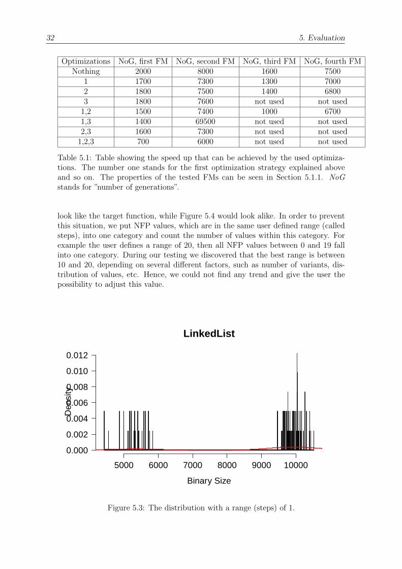
look like the target function, while Figure 5.4 would look alike. In order to preventthis situation, we put NFP values, which are in the same user defined range (calledsteps), into one category and count the number of values within this category. Forexample the user defines a range of 20, then all NFP values between 0 and 19 fallinto one category. During our testing we discovered that the best range is between10 and 20, depending on several different factors, such as number of variants, dis-tribution of values, etc. Hence, we could not find any trend and give the user thepossibility to adjust this value.

LinkedList

Binary Size

Den

sity

5000 6000 7000 8000 9000 10000

0.000

0.002

0.004

0.006

0.008

0.010

0.012

Figure 5.3: The distribution with a range (steps) of 1.


LinkedList

Binary Size

Den

sity

5000 6000 7000 8000 9000 10000

0e+00

2e−04

4e−04

6e−04

8e−04

Figure 5.4: The distribution with a range (steps) of 20. For the sake of clarity ofthe bars the range in the graph is higher but it was calculated using a range of 20.

Quantity of Population

The quantity of the population, which stays the same during all generations and isvery common among evolutionary algorithms, also has influence in the speed andaccuracy of the algorithm due to the fact that a bigger population requires a longerexecution time but also has a higher possibility of containing a good chromosome.As the user is free to adjust this value to its preferences a good compromise betweenspeed and accuracy is around 100 to 200 chromosomes. When having a FM with alower number of variants a population near 200 is advisable and vice versa.

Accuracy of the Resulting Distribution

The accuracy of the resulting distribution is used by one of the exit conditions. Thisvalue is the distance between the average growth of the distribution and the averagegrowth of the target function.Our tests are showing, that an accuracy of 6 is leading to an acceptable result.However, when lowering this value, better results are produced. But it is importantto notice, that during our testing process, we discovered that a bisection of this valuecan increase the number of generations by a factor of 2.Concluding, depending on the personal preference of the accuracy, a value of theinterval I =]0, 6] ∈ R can be chosen.

5.1.2 Input and Effects

In Chapter 4, we introduced the user adjustable properties concerning the featuremodel. This section focuses on the effects that different inputs have on NFP distri-butions of the feature models. Furthermore we give a recommendation on the bestinput for the desired distribution as not all different inputs can create all types of

34 5. Evaluation

distributions.The reason for that is fact that it is impossible to create a distribution with n ∈ Nbell-shaped curves using a FM with v < n variants (v ∈ N). Its distribution canonly have v peaks, meaning v bell-shaped curves.

Effects of Probabilities

As mentioned in Chapter 4 the four probabilities of a feature, being mandatory,optional, in an alternative relation or in an or relation, are completely adjustableby the user. This provides the possibility of generating all kinds of different initialdistributions. As the sum of these four probabilities has to be exactly 100 thereare four different basic ways of distributing the probabilities. Table 5.2 shows theseallocations and the resulting NFP distributions.These basic ways of distributing the probabilities are first of all to weight just oneof them. This is shown in the table at number 1 to 4. As can be noticed, the lessvariants a FM has, caused by a higher number of variant lowering properties suchas mandatory features, the higher the possibility of the distribution to be shapedlike a uniform distribution.Weighting two properties more than the others the results are quite the same as ahigher number of mandatory features and features that exclude each other lowersthe number of variants and provides the same distributions (to be seen at numbers5 to 10).Weighting three properties the strong variant lowering effects are smoothed so theresulting distributions are more likely to be shaped as a bell-shaped curve. Thesame is also true for weighting all properties the same.Concluding the results of these measurements are on the one hand that a very lownumber of variants (e.g. 8 or 20) result in a distribution shaping an equipartitionwhereas a high number of variant result in a distribution similar to one, two or morebell-shaped curves. On the other hand if the user desires a specific distribution type(e.g. an equipartition) then a FM creating a very similar initial distribution (e.g.a FM containing many mandatory features) is advisable. In individual cases theremight be another type of distribution as expected but these are exceptional cases.

Interactions

The feature generator also generates feature interactions, hence, we tested theirinfluences on NFP distributions. As this is not the main part of the evaluation, wejust focused on the potential of interactions to change an NFP distribution and donot give indepth explanation.In Chapter 3 we discovered during our analysis of real-world Datasets that about50 percent of all feature interactions had no influence on the NFP distribution dueto their NFP value of 0. The remaining 50 percent split into the following intervalsIx,y =]x · z, y · z] ∈ N with x, y ∈ [0, 1] ∈ R and z being the highest NFP value inthe FM: 15 percent of the NFP values of interactions v are v ∈ I0,0.3, 25 percent arev ∈ I0.3,0.7 and 10 percent v ∈ I0.7,1. (Section 3.2.1 in Chapter 3)Based on this data we tested the influence of interactions on the NFP distributionby taking the same FM with the same NFP values for the features and generateddifferent numbers and types of interactions onto this FM. It should be noted that


Num

ber

P.

Alt

ernat

ive

Rel

atio

nP

.O

rR

elat

ion

P.

Opti

onal

P.

Man

dat

ory

Typ

eof

Dis

trib

uti

on1

1010

70

10O

ne

and

Tw

ob

ell-

shp

edcu

rves

210

1010

70

Equip

arti

tion

370

1010

10E

quip

arti

tion

,O

ne

bel

l-sh

aped

curv

e4

1070

1010

One

and

Tw

ob

ell-

shap

edcu

rves

540

40

1010

One

and

Tw

ob

ell-

shap

edcu

rves

640

1040

10O

ne

and

Tw

ob

ell-

shap

edcu

rves

740

1010

40

Equip

arti

tion

,O

ne

bel

l-sh

aped

curv

e8

1040

40

10O

ne

and

Tw

ob

ell-

shap

edcu

rves

910

40

1040

Equip

arti

tion

,O

ne

and

Tw

ob

ell-

shap

edcu

rves

1010

1040

40

One

and

Tw

ob

ell-

shap

edcu

rves

1130

30

30

10O

ne

and

Tw

ob

ell-

shap

edcu

rves

1230

30

1030

One

and

Tw

ob

ell-

shap

edcu

rves

1330

1030

30

One

and

Tw

ob

ell-

shap

edcu

rves

1410

30

30

30

One,

Tw

oan

dT

hre

eb

ell-

shap

edcu

rves

1525

25

25

25

One

bel

l-sh

aped

curv

e

Tab

le5.

2:T

he

table

show

ing

the

resu

ltin

gdis

trib

uti

onre

spec

tive

toth

ein

put.

The

lett

er”P

”st

ands

for

pro

bab

ilit

y.T

he

mor

ew

eigh

ted

pro

per

ties

are

hig

hligh

ted.

The

valu

esar

egi

ven

inp

erce

nt.

The

num

ber

offe

ature

sw

as20

,an

dth

ep

erce

nta

geof

CT

Cs

and

Inte

ract

ions

wer

eke

pt

low

at0%

.T

he

list

eddis

trib

uti

ons

are

not

the

only

ones

that

are

gener

ated

by

the

give

ndat

abut

are

mos

tlike

lyto

be

shap

edlike

the

ones

men

tion

ed.

This

does

not

mea

nth

atit

isim

pos

sible

for

aF

Mw

ith

ahig

hnum

ber

ofm

andat

ory

feat

ure

s,fo

rex

ample

,to

hav

ea

dis

trib

uti

onsh

aped

asth

ree

bel

l-sh

aped

curv

ebut

itis

very

unlike

lyto

hap

pen

,as

sum

ing

that

the

NF

Pva

lues

are

equal

dis

trib

ute

d.

Hen

ce,

we

did

not

men

tion

them

.

36 5. Evaluation

the distribution of the feature interactions is following: 75% of the interactions areof first order, 20% are of second order and the remaining 5% are of third order.We chose this distribution due to the fact that this is the most common one [SBL].Figure 5.5 shows the NFP distribution of a FM without any feature interactions.The above mentioned distribution of NFP values concerning the feature interactionsleads to the guess that those have a small influence on the behavior of the NFPdistribution. However, when about 25% of all features are part of one or moreinteractions this behavior can dramatically change as seen in Figure 5.6. Listing5.1 shows the interactions belonging to Figure 5.6. It can be noticed that there areonly two interactions whose values are not 0 so those have the consequences thatthe NFP distribution changes. When increasing the number of features, interactingwith each other, the influence of these interactions is increasing, for obvious reasons.Figure 5.7 shows the FM with 75% of its features interacting with each other.Concluding this analysis shows that a higher number of interactions is leading to ahigher distraction of the distribution compared to the original one. This also explainsthe high number of NFP distributions shaped like three or more bell-shaped curvesdue to their interactions. Hence, we advise the users to include feature interactionsinto the generated FM when a NFP distribution consisting of several bell-shapedcurves is desired.

Figure 5.5: The NFP distribution of a Feature Model without any interactions. TheFM consists of 20 features, 10% CTCs and the probability of a feature being optionalis 70 %

Cross Tree Constraints

Cross Tree Constraints (CTC) limit the variability of a FM, when they are part ofone. During our testing process we discovered, that a higher amount of CTCs islowering the numbers of variants of the FM, thus, the probability of the FM, havinga NFP distribution that is shaped like an equal distributed function, is increasing.


Figure 5.6: The NFP distribution of a Feature Model with 25% of its features beingin an interaction. The FM consists of 20 features, 10% CTCs and the probability ofa feature being optional is 70%

Figure 5.7: The NFP distribution of a Feature Model with 75% of its features beingin an interaction. The FM consists of 20 features, 10% CTCs and the probability ofa feature being optional is 70 %

38 5. Evaluation

Listing 5.1: Interactions belonging to Figure 5.6



Additionally, we tested the effects of a high CTC value (40% and more of the fea-tures are part of a CTC) on the resulting NFP distribution, with the FM propertiesof Table 5.2.Our testing shows, that a percentage of 40% or higher of CTCs is increasing theprobability of equal distributions by a high value, as most of the properties, thatwould result in a one or two bell-shaped curve, resulted in most cases in an equaldistribution.Concluding, if the desired output of the algorithm is a NFP distribution that isshaped like an equal distributed function, but for example there have to be still 70%of the features optional, then increasing the percentage of CTCs is an option.

5.2 Evaluation of SAT Sampling

We evaluated the SAT sampling explained in Chapter 3 in order to ensure thecorrectness of the sampling distribution compared to the actual distribution. Weused the following setup for the evaluation process:We took a feature model with all of its NFP values randomly chosen but stayingthe same during the testing. The FM had no interactions as they do not influencethe SAT sampling.It is important to know that when SAT sampling is turned on, 5000 variants arepicked. We chose this number due to two reasons. First, when using a higher valuesuch as 10000 the execution time of the algorithm doubles, but at the same timethe accuracy is not doubling but growing considerably slower. Second, when usinga lower value such as 1000 the accuracy of the sampling is affected too much due tojust having one eighth of the original number of variants.As a conclusion 5000 variants is a good compromise between time and accuracy, butthis is only a reference value we defined so the user is free to change this number.Figure 5.8 shows the big aberration between the sampled distribution and the actualdistribution.

In order to test the aberration of the distributions, we first generated all possiblevariants of the FM, calculated their NFP values and then translated this informationinto an NFP distribution. Second we used the SAT sampling to choose 10000, 5000and 1000 variants and generated the corresponding NFP distributions. Afterwardswe compared those by their distance of average growth. This process was done forevery FM we tested. The following figure (Figure 5.9) shows the aberration betweenthe actual and the 5000 variant distributions of a FM. The aberration stayed verysimilar for all tested FMs.

5.2. Evaluation of SAT Sampling 39

SAT Sampling

Performance Values

Den

sity

100 200 300 400 500 600 700 800

0.00

00.

002

0.00

4

426881000050001000

426881000050001000

Figure 5.8: The NFP distributions of a Feature Model consisting of 20 features. Theblue line represents the distribution among all variants, the red line the one among5000 variants, the green one line among 5000 and the yellow one among 1000.

SAT Sampling

Performance Values

Den

sity

200 400 600 8000.00

000.

0015

0.00

30 42688 variants5000 variants

Figure 5.9: The NFP distributions of a Feature Model consisting of 20 features. Theblue line represents the distribution among all variants, the red line the one among5000 variants.

40 5. Evaluation

The difference between the distribution containing all variants and the one contain-ing only 5000 is noticeable in the slight shifting of the whole function to the left. Theactual shape of a one bell-shaped curve stayed the same recognizable by the similarheight and width. Even though the FM with the sampled variants only consists ofone eighth of the actual number of variants, the average aberration is 2.3 in thisexample. The other tested FMs also had an aberration of about 2.

6. Related Work

The subject of this thesis is relatively unexplored, what laid the basis for the moti-vation. There are, however, some papers to be considered as related work.Soltani et al. generated an NFP distribution for their testing process by assign-ing NFP values to features that were produced by a random function with normaldistribution. Depending on the number of variants and other factors, this distribu-tion could result in an NFP distribution shaping, e.g. a bell-shaped curve. As thismethod, however, does not always produce real-world NFP distributions, e.g. it alsocould produce a distribution shaped as a linear growing function, our approach dif-fers in that it always provides a user selectable real-world-based distribution [Sol12].Segura et al. described the functionality of their testing and benchmarking toolcalled BeTTy and also emphasized the necessity of a testing tool for automatedanalysis of feature models. Their tool is a test suite, which is generating a useradjustable feature model, containing NFP values, and the corresponding correctproperties of the FM (e.g. number of possible variants). Afterwards testing of anal-ysis methods is done by giving the method the generated FM and comparing itsoutput with the correct output created by BeTTy. Their approach of generatingNFP values is very similar to the one Soltani et al. are using. They assign NFP val-ues to features by a random function with pre-defined distributions. This differs toour approach in that we create real-world-based NFP values. Additionally, we addfeature interactions to our generated FM. Hence, we create an even more realisticfeature model generator [SGB+12].Segura et al. also created a test suite called FaMa, which provides a set of test-casesin order to test analysis tools. Those test-cases are implementation independent,thus, providing a useful test suite. As this is the predecessor of BeTTy, however,they neither did include NFP values nor feature interactions, which separates thiswork from our approach. [SBRC10]Segura et al. also had another approach of automatically generating test data foranalysis tool by using a existing FM as a basis. This works by using a set ofmetaphoric relations and a test data generator. The generator then, is capable ofgenerating neighbor FMs of the given FM, when knowing its set of products. Unfor-tunately, they also do not include NFP values or feature interactions. [SHBRC10]

42 6. Related Work

Concluding the subject of testing with real-world NFP distributions is not jet fullydiscovered, thus, leaving a big gap and a huge need for further research. With ourwork we fill this gap, so further work will be inspired by our approach.

7. Conclusion

In this thesis we developed a test suite for the creation of a user adjustable FM witha user selectable real-world based NFP distribution.The subject of this thesis stems from the need of a test suite for generating user ad-justable feature models with real-world based NFP distributions. In order to proofthis necessity, we analyzed the testing process of methods (which is described inliterature) that analyze on feature models. As a result, we discovered that a vastmajority of the methods are tested with random NFP distributions, thus, makingit impossible to have confidence in the analysis results of those methods. Only onepaper is using a different approach. Unfortunately, all papers analyzed, also do notinclude feature interactions in their FMs.Additionally to the analysis of literature, we also analyzed the different types ofNFP distributions of real-world datasets, in order to have reference functions ourtest suite can orientate on. Furthermore, we examined the typical behavior of NFPvalues of feature interactions, which differs from the one of features. All this dataprovided a basis for the creation and optimization of the resulting test suite.This suite is a tool, which fills the wide open gap of testing tools and offers aneasy and comfortable way of generating FMs, containing feature interactions, withreal-world based NFP distributions. It offers a wide range of FMs due to the manyuser adjustable settings. The heart of this tool, an evolutionary algorithm, thentransforms those settings into a FM containing the desired NFP distribution. Ad-ditionally one of the benefits of an evolutionary algorithm is the room for furtherimprovements, hence, there is a huge potential for a later enhancement of user ex-perience.Afterwards, we evaluated our work, in particular the optimization strategies and theSAT sampling and additionally examined the effects of feature interactions and dif-ferent types of FMs (e.g. FM with 20% optional features vs. FM with 70% optionalfeatures) on an NFP distribution.With this test suite, testing can be easily done using real-world NFP distributionsin order to ensure that the analysis tool, using this suite, is armed for all real-worldsituations.

44 7. Conclusion

8. Future Work

In this chapter, we focus on the work that could be done in the future in order toimprove the algorithm or other components.

8.1 Fitness Function

The fitness function is one essential and critical part of an evolutionary algorithm,hence, there is a huge potential for improvement in all of its components, that cannot be exploited to the full in this thesis. Reasons for that are time limitations,complexity and need for further research.

8.1.1 Initial Population

The initial population, defined in Chapter 4, has the task to randomly generate NFPvalues in order to assign those to the features and interactions contained in the be-fore generated FM. This corresponds to the usual implementation of an evolutionaryalgorithm. However, there is another approach of generating an initial populationwhich distributes NFP values very concerted in order to generate an initial pop-ulation containing chromosomes that already have a very high similarity with thedesired output. This reduces the execution time. [SHF+94]Implementing this approach, we first would have to examine how the NFP values ofthe features have to be distributed when a certain NFP distribution of the variantsis desired. That means, we would have to identify the typical NFP distribution ofthe features that leads to a certain NFP distribution of the variants. Thereby notonly the NFP distribution of the features but also the number and composition ofall possible variants have to be taken into account as they also influence the distri-bution of the variants.

46 8. Future Work

8.1.2 Generating Functions

In Chapter 5, we explain the different metrics and their assets and drawbacks inmatters of the comparison between the generated distribution and the target func-tion. It also emphasizes the fact that we are limited in those metrics due to thecircumstance that the generated distribution is described by a discrete key-valuepair.When we could generate a function out of this key-value pair, however, the compar-ison between the two functions would be much more accurate due to the possibilityof using an integral or other metrics to compare those. This would boost the accu-racy of the fitness function, thus, providing the basis for even better optimizationtechniques.We know that this is already possible but only in a limited matter.

8.2 Optimization through Parallelization

The execution time is always a critical factor due to having very large populations,chromosomes with many genes, which is a high constant factor when comparingchromosomes, etc. Thus, it is advisable to parallelize some of the execution steps,as evolutionary algorithms are easily parallelized [Mit97].When parallelizing, the following concepts can be used to improve execution time.The idea of this concept is to split the chromosomes into groups called demes andassign each core of a processor a deme. For all chromosomes the fitness is calcu-lated regularly but a crossover between chromosomes of one deme are more likelyto happen than between chromosomes of different demes [Tan89], [CHMR87]. Asa benefit not only one local optimum would dominate the next generations but awider variety of chromosomes would arise and might lead to a bigger variety of evenbetter chromosomes in the next generations.

8.3 Mutation and Crossover

Mutation and crossover are the instruments of an evolutionary algorithm to generatethe chromosomes of the next generation with a higher fitness then their predecessors.Hence, there are several different approaches of those operations. The variants usedin this thesis are called ”single-point crossover” and ”point mutation” and explainedin Chapter 4.In a future work different crossover and mutation types like ”uniform crossover”,where not only one set of genes is exchanged but several ones, of different length,can be tested [Mit97]. Also normal distributed mutation, where the gene beingmutated is selected by a random number which is normal distributed, is an option[SHF+94].Additionally other optimization instruments, such as operators using domain spe-cific rules, can be introduced [Jan93]. Those have the ability of changing single genesnot randomly but tailored to the target function, in order to generate a chromosomewith a higher fitness.

8.4. Extending the Feature Model 47

8.4 Extending the Feature Model

Feature Models can have several different components, such as features with NFPvalues and CTC. In future work the components we use in this thesis can be ex-tended. In particular numeric features and NFP values which are composed of theNFP values of other features. All those improvements would lead to a generation ofeven more realistic feature models, thus, improving the quality of the test suite.

48 8. Future Work

A. Appendix

Visual Representation of the NFP distributions

This is an additionally section to inform the reader about the problem, we had withthe visual representation of the NFP distributions. In order to visualize those, weused the statistical program called R. When generating the histogram of the belowseen NFP distributions, the only way of displaying this red density curve, was tochange the representation of the y-axis. This went from displaying the frequency ofthe values of the x-axis, to displaying the density of those. This means, that thesum of the area of all bars adds up to 1 and therefore, the values of the y-axis arenot as expected. Until the deadline of this thesis, we unfortunately did not find anysolution to that problem.This problem is, however, not as problematic, due to the fact that the course of thefunction is visible, which is the main purpose of those histograms in the subject ofthis thesis.

Implementation Dependent Constraints

When starting the graphical user interface (GUI) of this test suite, the user will beprompted to enter some property values for the FM. Hereby, it is important to notice,that the sum of the probabilities of a feature being optional, being mandatory, arepart in an or and alternate relation have to add up to exactly 100%.the same is true for changing the percentages of interactions of different order. Thosethree values also have to sum up to 100%. Additionally, when the user wants tochange those values the check mark above has to be checked.When the user enters the settings of the algorithm, and is prompted to enter thetarget function, there are some constraints to be noticed:

• The variable of the function has to be named x. For example 2 ∗ x. It mustnot be another name like ”y”.

50 A. Appendix

• When calculating the maximum of two or more functions, then the word ”max”has to be used and the functions have to be surrounded by brackets and sep-arated by commas, like ”max(a,b,c)”. The same goes for the minimum, as theword is ”min”.

When including all the extern libraries, in order to run the program, the user needsto have the program R installed and furthermore the library called JRI has to beinstalled. The installation process is depending on the operating system, thus, weadvice the user to use the provided installation guide 1.As an important notice: The file called ”FMInteractionEinlesen.R” has to be in thesame path, the program is executed from.

A.1 All analyzed real-world NFP Distributions

In this section, we list all the analyzed real-world NFP distributions together withsome additional information.Due to a Latex bug, the remaining NFP distribution could not be loaded. However,all distributions are also contained in a digital form on a CD.Due to bugs in SPLConqueror, some variants were not calculated and some datawas not accepted at all.

BerkeleyC - NFP: Binary Size

• Number of Features 18

• Number of Mandatory Fea-tures 2

• Number of Optional Fea-tures 7

• Number of Features in OrRelations 0

• Number of Features in Al-ternative Relations 9

• Number of Variants 2560

1http://rforge.net/JRI/

A.1. All analyzed real-world NFP Distributions 51

PrevaylerPP - NFP: Binary Size







SQLite - NFP: Binary Size






• Number of Variants not ap-plicable

mEPL - NFP: Binary Size

• No Data found!

52 A. Appendix

LinkedList - NFP: Binary Size

• No data found!

mPKJab - NFP: Binary Size







mZipMe - NFP: Binary Size








SQLite - NFP: MemoryConsumption







WGet - NFP: MemoryConsumption







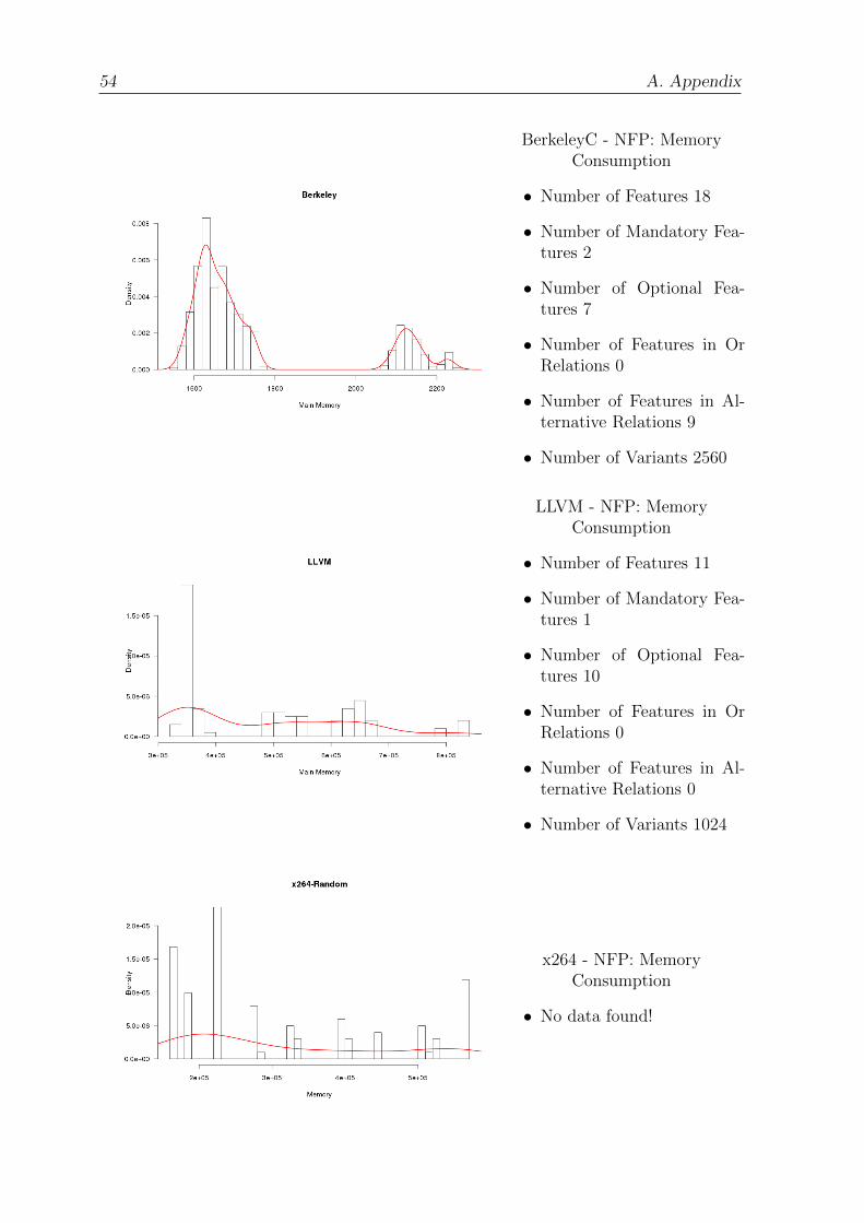
54 A. Appendix

BerkeleyC - NFP: MemoryConsumption







LLVM - NFP: MemoryConsumption







x264 - NFP: MemoryConsumption

• No data found!


SQLite - NFP: Performance







Email - NFP: Performance







Apache - NFP: Performance







56 A. Appendix

h264 - NFP: Performance







BerkeleyC - NFP: Performance







BerkeleyJ - NFP: Performance







Bibliography

[ABM+13] Micha l Antkiewicz, Kacper B ↪ak, Alexandr Murashkin, RafaelOlaechea, Jia Hui (Jimmy) Liang, and Krzysztof Czarnecki. Clafertools for product line engineering. Proceedings of the 17th Interna-tional Software Product Line Conference co-located workshops on -SPLC ’13 Workshops, page 130, 2013. (cited on Page 8)

[Ale03] Ian Alexander. Misuse cases help to elicit non-functional requirements.Computing and Control . . . , pages 1–10, 2003. (cited on Page 8)

[BMO09] Joerg Bartholdt, Marcel Medak, and Roy Oberhauser. IntegratingQuality Modeling with Feature Modeling in Software Product Lines.2009 Fourth International Conference on Software Engineering Ad-vances, pages 365–370, September 2009. (cited on Page 8)

[BTRC05a] David Benavides, Pablo Trinidad, and A Ruiz-Cortes. Automated rea-soning on feature models. Advanced Information Systems . . . , 01:491–503, 2005. (cited on Page 8 and 9)

[BTRC05b] David Benavides, Pablo Trinidad, and Antonio Ruiz-Cortes. Auto-mated reasoning on feature models. In Advanced Information SystemsEngineering, pages 491–503. Springer, 2005. (cited on Page 1 and 2)

[CdPL09] Lawrence Chung and Julio Cesar Sampaio do Prado Leite. On non-functional requirements in software engineering. In Conceptual mod-eling: Foundations and applications, pages 363–379. Springer, 2009.(cited on Page 8)

[CE00] Krzysztof Czarnecki and Ulrich W Eisenecker. Generative program-ming. 2000. (cited on Page 5)

[CHMR87] James P Cohoon, Shailesh U Hegde, Worthy N Martin, andD Richards. Punctuated equilibria: a parallel genetic algorithm. InProceedings of the Second International Conference on Genetic Algo-rithms on Genetic algorithms and their application, pages 148–154. L.Erlbaum Associates Inc., 1987. (cited on Page 46)

[CKMRM03] Muffy Calder, Mario Kolberg, Evan H Magill, and Stephan Reiff-Marganiec. Feature interaction: a critical review and considered fore-cast. Computer Networks, 41(1):115–141, 2003. (cited on Page 7)

58 Bibliography

[CPFD01] Denis Conan, Erik Putrycz, Nicolas Farcet, and Miguel DeMiguel. In-tegration of non-functional properties in containers. In Proceedings ofthe Sixth International Workshop on Component-Oriented Program-ming (WCOP), volume 1, page 2, 2001. (cited on Page 8)

[EMB07] Leire Etxeberria, GS Mendieta, and Lorea Belategi. Modelling Vari-ation in Quality Attributes. VaMoS, 2007. (cited on Page 8)

[GWW+11] Jianmei Guo, Jules White, Guangxin Wang, Jian Li, and YinglinWang. A genetic algorithm for optimized feature selection with re-source constraints in software product lines. Journal of Systems andSoftware, 84(12):2208–2221, December 2011. (cited on Page 9)

[Jan93] Cezary Z Janikow. A knowledge-intensive genetic algorithm for su-pervised learning. Machine Learning, 13(2-3):189–228, 1993. (cited

on Page 46)

[KAK09] Christian Kastner, Sven Apel, and Martin Kuhlemann. A Modelof Refactoring Physically and Virtually Separated Features. In Pro-ceedings of the International Conference on Generative Programmingand Component Engineering (GPCE), pages 157–166. ACM, October2009. (cited on Page 2)

[MARC13] Alexandr Murashkin, Micha l Antkiewicz, Derek Rayside, andKrzysztof Czarnecki. Visualization and exploration of optimal vari-ants in product line engineering. Proceedings of the 17th InternationalSoftware Product Line Conference on - SPLC ’13, page 111, 2013.(cited on Page 9)

[Mit97] Tom M Mitchell. Machine learning. wcb, 1997. (cited on Page 9 and 46)

[RFBRC+11] Fabricia Roos-Frantz, David Benavides, Antonio Ruiz-Cortes, AndreHeuer, and Kim Lauenroth. Quality-aware analysis in product lineengineering with the orthogonal variability model. Software QualityJournal, 20(3-4):519–565, August 2011. (cited on Page 9)

[RFBRC+12] Fabricia Roos-Frantz, David Benavides, Antonio Ruiz-Cortes, AndreHeuer, and Kim Lauenroth. Quality-aware Analysis in Product LineEngineering with the Orthogonal Variability Model. Software QualityJournal, 20(3-4):519–565, 2012. (cited on Page 1)

[RNMM08] Mikko Raatikainen, E Niemela, V Myllarniemi, and T Mannisto.Svamp-An Integrated Approach for Modeling Functional and Qual-ity Variability. VaMoS, 2008. (cited on Page 9)

[SBL] Gunter Saake, Don Batory, and Christian Lengauer. Measuring andpredicting non-functional properties of customizable programs. (cited

on Page 36)

Bibliography 59

[SBRC10] Sergio Segura, David Benavides, and Antonio Ruiz-Cortes. Fama testsuite v1. 2. ISA Research Group, 2010. (cited on Page 41)

[SGB+12] S. Segura, J.A. Galindo, D. Benavides, J.A. Parejo, and A. Ruiz-Cortes. Betty: Benchmarking and testing on the automated analysisof feature models. In U.W. Eisenecker, S. Apel, and S. Gnesi, editors,Sixth International Workshop on Variability Modelling of Software-intensive Systems (VaMoS’12), page 63–71, Leipzig, Germany, 2012.ACM, ACM. (cited on Page 20 and 41)

[SHBRC10] Sergio Segura, Robert M Hierons, David Benavides, and AntonioRuiz-Cortes. Automated Test Data Generation on the Analyses ofFeature Models: A Metamorphic Testing Approach. In SoftwareTesting, Verification and Validation (ICST), 2010 Third InternationalConference on, pages 35–44. IEEE, 2010. (cited on Page 41)

[SHF+94] Eberhard Schoneburg, Frank Heinzmann, Sven Feddersen, et al.Genetische algorithmen und evolutionsstrategien. Bonn: Addison-Wesley, 1994. (cited on Page 9, 45, and 46)

[SIMA13] Abdel Salam Sayyad, Joseph Ingram, Tim Menzies, and Hany Am-mar. Scalable product line configuration: A straw to break the camel’sback. 2013 28th IEEE/ACM International Conference on AutomatedSoftware Engineering (ASE), pages 465–474, November 2013. (cited

on Page 9)

[SKK+12] Norbert Siegmund, Sergiy S Kolesnikov, Christian Kastner, SvenApel, Don Batory, Marko Rosenmuller, and Gunter Saake. Predictingperformance via automated feature-interaction detection. In Proceed-ings of the 34th International Conference on Software Engineering,pages 167–177. IEEE, 2012. (cited on Page 11)

[Sol12] Samaneh Soltani. Towards automated feature model configurationwith optimizing the non-functional requirements. 2012. (cited on

Page 9 and 41)

[SRK+11] Norbert Siegmund, Marko Rosenmuller, Christian Kastner, Paolo GGiarrusso, Sven Apel, and Sergiy S Kolesnikov. Scalable predictionof non-functional properties in software product lines. In SoftwareProduct Line Conference (SPLC), 2011 15th International, pages 160–169. IEEE, 2011. (cited on Page 11)

[SRK+13] Norbert Siegmund, Marko Rosenmuller, Christian Kastner, Paolo GGiarrusso, Sven Apel, and Sergiy S Kolesnikov. Scalable predic-tion of non-functional properties in software product lines: Footprintand memory consumption. Information and Software Technology,55(3):491–507, 2013. (cited on Page 11)

60 Bibliography

[SRP] D. Streitferdt, M. Riebisch, and K. Philippow. Details of formalizedrelations in feature models using OCL. 10th IEEE International Con-ference and Workshop on the Engineering of Computer-Based Sys-tems, 2003. Proceedings., pages 297–304. (cited on Page 9)

[SvRA13] Norbert Siegmund, Alexander von Rhein, and Sven Apel. Family-based performance measurement. In Proceedings of the 12th interna-tional conference on Generative programming: concepts & experiences,pages 95–104. ACM, 2013. (cited on Page 11)

[Tan89] Reiko Tanese. Distributed genetic algorithms. In Proceedings of thethird international conference on Genetic algorithms, pages 434–439.Morgan Kaufmann Publishers Inc., 1989. (cited on Page 46)

[WDS09] Jules White, Brian Dougherty, and DC Schmidt. Selecting highlyoptimal architectural feature sets with filtered cartesian flattening.Journal of Systems and Software, (August 2008):1–36, 2009. (cited

on Page 9)

[WSNW] Jules White, Douglas C Schmidt, Andrey Nechypurenko, and EgonWuchner. Optimizing and Automating Product-Line Variant Selectionfor Mobile Devices. (cited on Page 9)

Eidesstattliche Erklarung:

Hiermit versichere ich an Eides statt, dass ich diese Bachelorarbeit selbstandig undohne Benutzung anderer als der angegebenen Quellen und Hilfsmittel angefertigthabe und dass alle Ausfuhrungen, die wortlich oder sinngemaß ubernommen wur-den, als solche gekennzeichnet sind, sowie dass ich die Masterarbeit in gleicher oderahnlicher Form noch keiner anderen Prufungsbehorde vorgelegt habe.

Name

Passau, den 27. Juni 2014

Generating Realistic non-functional Property Attributes ...

Documents

Transcript of Generating Realistic non-functional Property Attributes ...