Generalized Ultrametric Spaces in

Quantitative Domain Theory

Markus Krotzsch

Knowledge Representation and Reasoning Group, Artificial Intelligence InstituteDepartment of Computer Science, Dresden University of Technology

Dresden, Germany1

mak@aifb.uni-karlsruhe.de

Technical Report WV-04-02

AbstractDomains and metric spaces are two central tools for the study of denotational semantics

in computer science, but are otherwise very different in many fundamental aspects. Aconstruction that tries to establish links between both paradigms is the space of formalballs, a continuous poset which can be defined for every metric space and that reflectsmany of its properties. On the other hand, in order to obtain a broader framework forapplications and possible connections to domain theory, generalized ultrametric spaces(gums) have been introduced. In this paper, we employ the space of formal balls as a toolfor studying these more general metrics by using concepts and results from domain theory.It turns out that many properties of the metric can be characterized by conditions on itsformal-ball space. Furthermore, we can state new results on the topology of gums as wellas two modified fixed point theorems, which may be compared to the Prieß-Crampe andRibenboim theorem and the Banach fixed point theorem, respectively. Deeper insights intothe nature of formal-ball spaces are gained by applying methods from category theory.Our results suggest that, while being a useful tool for the study of gums, the space offormal balls cannot provide the hoped-for general connection to domain theory.

Contents

1 Introduction 2

2 Related work 3

3 Preliminaries and notation 33.1 Partial orders . . . . . . . . . . . . . . . . . . . . . . . . . . . . . . . . . . . . 33.2 Generalized ultrametric spaces . . . . . . . . . . . . . . . . . . . . . . . . . . 43.3 Domains . . . . . . . . . . . . . . . . . . . . . . . . . . . . . . . . . . . . . . . 63.4 Topological spaces . . . . . . . . . . . . . . . . . . . . . . . . . . . . . . . . . 73.5 Categories . . . . . . . . . . . . . . . . . . . . . . . . . . . . . . . . . . . . . . 7

4 The poset BX 94.1 Continuity of BX . . . . . . . . . . . . . . . . . . . . . . . . . . . . . . . . . . 104.2 The Scott-topology on BX . . . . . . . . . . . . . . . . . . . . . . . . . . . . 12

5 Categories of gums 17

6 Fixed point theorems 22

1Current affiliation: Institute AIFB, Universitat Karlsruhe

1

7 Summary and conlcusion 25

1 Introduction

Domain theory and the theory of metric spaces are the two central utilities in the study ofdenotational semantics in computer science. Although both formalisms are capable of captur-ing the relevant aspects of computation and approximation, they do so in very different ways.Consequently, various methods for relating both paradigms have been sought, establishing aline of research that is now known as quantitative domain theory.

In [5], a construction for obtaining a partially ordered set from a given (classical) metricspace was introduced. This order was called the space of formal balls and was shown to bea continuous poset with properties closely related to the metric from which it originated. Itcould also be shown that the space of formal balls can be employed as a tool for proving knownresults for metric spaces, and that it yields a computational model for the metric topology.In [12], the concept of a formal-ball space was then extended to the setting of generalizedultrametric spaces (gums), i.e. non-Archimedian metrics that can have sets of distances otherthan the real numbers. Restricting to gums with (linearly ordered) ordinal distance sets, aconstructive proof of the Prieß-Crampe and Ribenboim fixed point theorem (see [16]) couldbe obtained.

However, beyond this result, little is known about the space of formal balls for generalizedultrametric spaces, especially in the situation where no additional restrictions are imposed onthe distance set. Thus, an initial objective of this work will be to establish detailed relationsbetween these concepts, following the lines of [5]. In Section 4, we shall see that complete-ness and continuity of formal ball spaces can indeed be characterized in a convenient way.Furthermore, as in the case of classical metric spaces, the space of formal balls can serve as acomputational model for the metric topology of a gum. As a side effect, this will shed somelight on the role of the open ball topology for gums.

Another central question that is to be addressed in this paper is whether the constructionof spaces of formal balls can connect the theory of gums and domain theory in a generalsense. For this purpose, we will call upon the formalism of category theory in Section 5 andestablish a categorical equivalence between suitable categories of gums on the one hand andpartially ordered sets on the other. It will turn out that the spaces of formal balls actuallyform a very restricted class of partial orders and the utility of this approach to quantitativedomain theory may thus be doubted.

Finally, in Section 6, we present two fixed point theorems for gums, which are comparedwith the Prieß-Crampe and Ribenboim theorem and the Banach fixed point theorem, respec-tively. Together with the former application of the space of formal balls for the investigationof the metric topology, this demonstrates the use of this construction as a tool for obtainingproofs.

During our considerations, we will also introduce numerous restrictions on the very gen-eral definition of gums. Since these restrictions often give tight characterizations of certaindesirable situations, they may turn out to be useful for choosing reasonable settings for futureinvestigations of gums.

2

2 Related work

In the search for connections between domain theory and the theory of metric spaces variousdifferent notions of “generalized” metrics have been introduced. One way to represent ordersdirectly is to allow the distance function to be non-symmetric, and setting d(x, y) = 0 if x ≤ yand d(x, y) = 1 otherwise. This connection has first been investigated and extended by Smyth[19]. Metrics that arise by discarding both symmetry and the property that d(x, y) = 0 impliesx = y also appear under the label “generalized metrics” in this line of research. Another lessambiguous name for these structures is quasi-pseudo-metrics.

A second approach to quantitative domain theory is to generalize the set of distances,again combined with non-symmetric distance mappings. This was pioneered by Kopperman[13] and subsequently extended by Flagg [6], who proposed value quantales as appropriatestructures to generalize the real numbers that are employed in the classical case.

In fact, these abstractions of quasi-metric spaces can be captured in the uniform frame-work of enriched category theory, where one considers categories for which the Hom-functoris allowed to map to categories other than Set. In this framework, preorders also appear asspecial categories, enriched over the finite category {0, 1}. These connections have been stud-ied in various papers by Bosangue, van Breugel, and Rutten [3]. We also mention [17], where– among other results – the author defines a different order of formal balls that is comparedto the one from [5].

Another line of research focuses on symmetric real-valued distances but relaxes the reflex-ivity condition to allow non-zero self distances. This leads to the concept of a partial metric,which has been studied in [14], [15], [18], and [21], to name a few. Although these metricsare symmetric, they capture both order and topology in a natural way. The advantage of thisapproach is that, while being not as general as the abstract approaches related to enrichedcategory theory, it often allows for simpler constructions. For instance one may obtain theScott-topology without the need for an auxiliary topology.

Generalized ultrametric spaces in the sense of this work were introduced into the studyof logic programming semantics in [16], where they are just called “ultrametric spaces”. Con-nections to domain theory using the space of formal balls were first studied in a series ofpublications of Hitzler and Seda [9, 10, 11, 12] where the authors apply generalized ultramet-ric spaces to obtain fixed point semantics for various classes of logic programs.

3 Preliminaries and notation

In this section, we provide basic definitions of various concepts that are needed below. Besidesome remarks on notation, it is concerned with the fundamentals of generalized ultrametricspaces, domain theory, topology, and category theory.

3.1 Partial orders

For the basic notions of order theory we recommend [4] as a standard reference. We assumethe reader to be familiar with the corresponding notions and restrict to some remarks on thenotation that we will employ below.

For a partially ordered set Γ, we use Γ∂ to denote the order dual of Γ. Care will be takento clarify to what version of a poset a given order-theoretic property or limit-constructionrefers to. For this purpose, we will sometimes use notations such as ≤∂ .

3

Since we will have to deal with more than one order most of the time, we will be carefulto distinguish between the according constructions. For instance, least upper bounds withinthe orders ≤, ⊑, and ≤∂ will be denoted by

∨

,⊔

, and∨∂ , respectively.

For a partial order ≤, < will be used to denote the strict order induced by ≤.

3.2 Generalized ultrametric spaces

Definition 3.1 Let X be a set and let (Γ,≤) be a partially ordered set with least element⊥. (X, d,Γ) is a generalized ultrametric space (gum) if d : X ×X → Γ is a function such that,for all x,y,z ∈ X and all γ ∈ Γ, we have:

(U1) d(x, y) = ⊥ implies x = y.

(U2) d(x, x) = ⊥.

(U3) d(x, y) = d(y, x).

(U4) If d(x, y) ≤ γ and d(y, z) ≤ γ, then d(x, z) ≤ γ.

These properties will be called identity of indiscernibles (U1), reflexivity (U2), symmetry(U3), and the strong triangle inequality (U4), respectively. The poset Γ will be referred to asthe set of distances of a gum. In the following we will only consider gums where the set ofpoints X is non-empty.

The next definition introduces an important tool in our study of generalized ultrametricspaces, which was first defined for the general case in [8] and [12]. It is motivated by a similarconstruction for classical metric spaces, that was introduced in [5].

Definition 3.2 Let (X, d,Γ) be a generalized ultrametric space. We define an equivalencerelation ≈ on X × Γ by setting (x, α) ≈ (y, β) iff α = β and d(x, y) ≤ α.

The space of formal balls (BX,⊑) is an ordered set, where BX = (X × Γ)|≈ is the setof all ≈-equivalence classes and, for all [(x, α)], [(y, β)] ∈ BX, we have [(x, α)] ⊑ [(y, β)] iffβ ≤ α and d(x, y) ≤ α.

It is easy to see that (BX,⊑) is a well-defined partially ordered set. In the following,(X, d,Γ) will be a generalized ultrametric space and BX will be used to abbreviate its spaceof formal balls. Sets of the form {y | d(x, y) ≤ α} will be called closed ball with center x andradius α and are denoted by Bα(x). Similarly, open balls are sets of the form Bα(x) = {y |d(x, y) < α}.

Definition 3.3 A gum (X, d,Γ) is

(i) spherically complete if every non-empty chain C of closed balls of X, ordered by subsetinclusion, has non-empty intersection

⋂

C 6= ∅,

(ii) chain-spherically complete if every non-empty chain C of closed balls of the form C ={Bβ(xβ) | β ∈ Λ}, where Λ is a chain in Γ, has non-empty intersection.

Note that any chain of closed balls whose set of radii is a chain in Γ has a form as in(ii), since any two ⊆-comparable balls with the same radius coincide. This is an immediateconsequence of the fact that every point inside a closed ball is also its center, a well-knownfact for ultrametrics (see also [8]).

4

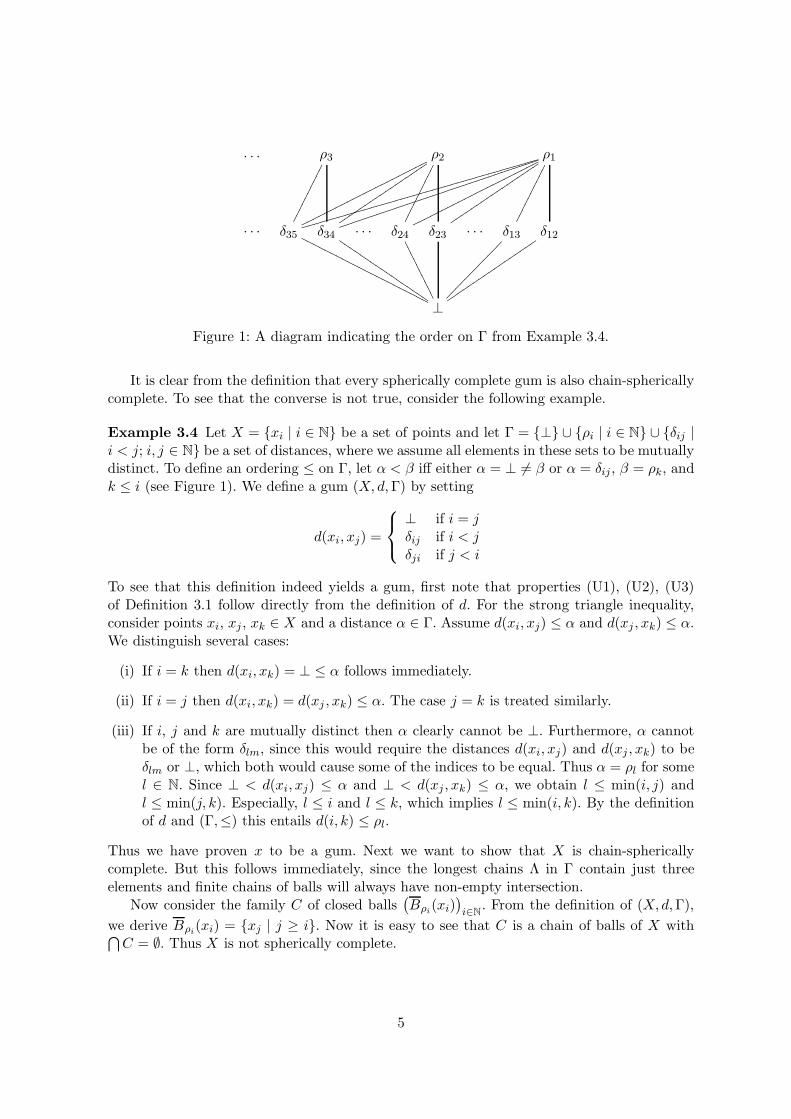
. . . ρ3

����������

ρ2

����������

uuuuuuuuuuuuuuuuu

ooooooooooooooooooooooρ1

����������

uuuuuuuuuuuuuuuuu

oooooooooooooooooooooo

jjjjjjjjjjjjjjjjjjjjjjjjjjjjjjjj

hhhhhhhhhhhhhhhhhhhhhhhhhhhhhhhhhhhhhh

. . . δ35

OOOOOOOOOOOOOOOOOOOOOO δ34

IIIIIIIIIIIIIIIII. . . δ24

////

////

//δ23 . . . δ13

����

����

����

δ12

uuuuuuuuuuuuuuuuu

⊥

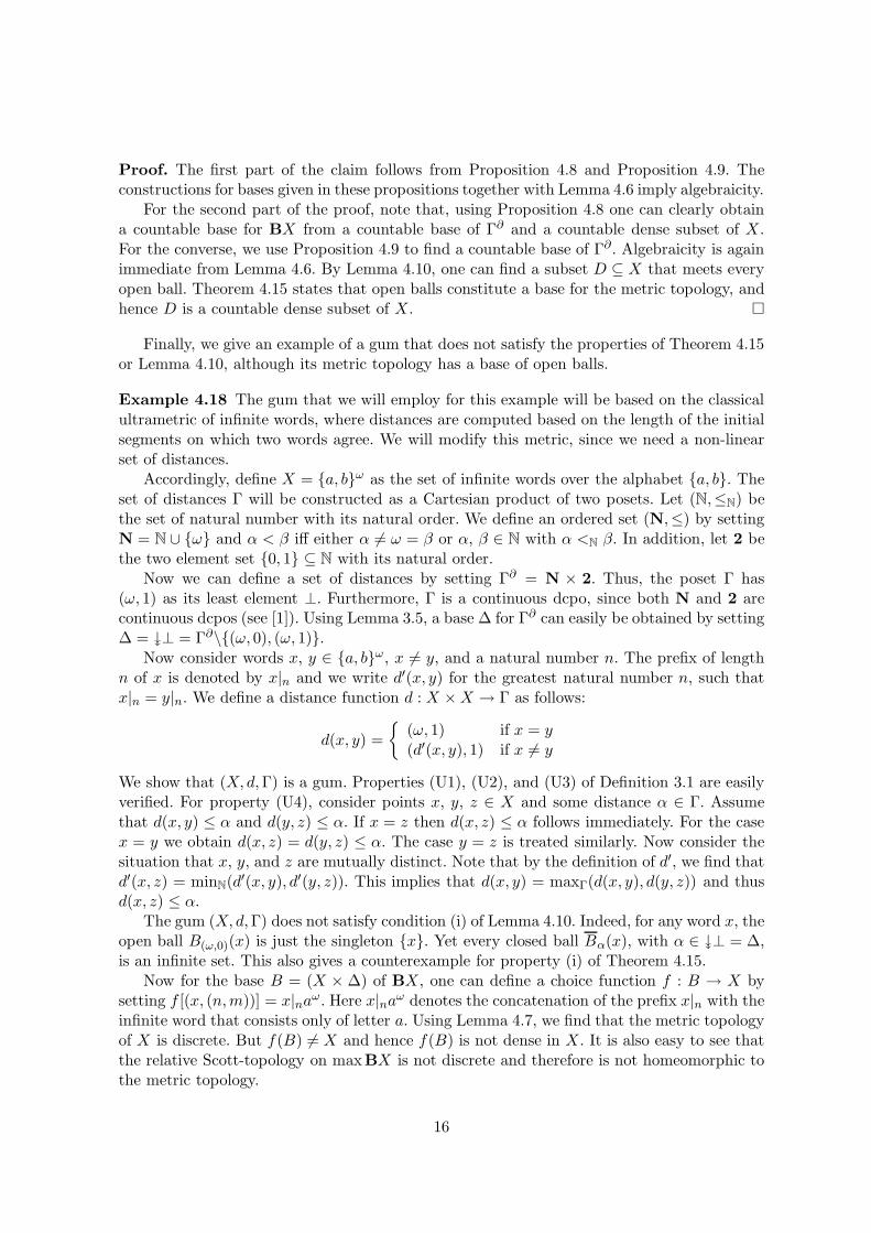
Figure 1: A diagram indicating the order on Γ from Example 3.4.

It is clear from the definition that every spherically complete gum is also chain-sphericallycomplete. To see that the converse is not true, consider the following example.

Example 3.4 Let X = {xi | i ∈ N} be a set of points and let Γ = {⊥} ∪ {ρi | i ∈ N} ∪ {δij |i < j; i, j ∈ N} be a set of distances, where we assume all elements in these sets to be mutuallydistinct. To define an ordering ≤ on Γ, let α < β iff either α = ⊥ 6= β or α = δij , β = ρk, andk ≤ i (see Figure 1). We define a gum (X, d,Γ) by setting

d(xi, xj) =

⊥ if i = jδij if i < jδji if j < i

To see that this definition indeed yields a gum, first note that properties (U1), (U2), (U3)of Definition 3.1 follow directly from the definition of d. For the strong triangle inequality,consider points xi, xj , xk ∈ X and a distance α ∈ Γ. Assume d(xi, xj) ≤ α and d(xj , xk) ≤ α.We distinguish several cases:

(i) If i = k then d(xi, xk) = ⊥ ≤ α follows immediately.

(ii) If i = j then d(xi, xk) = d(xj , xk) ≤ α. The case j = k is treated similarly.

(iii) If i, j and k are mutually distinct then α clearly cannot be ⊥. Furthermore, α cannotbe of the form δlm, since this would require the distances d(xi, xj) and d(xj , xk) to beδlm or ⊥, which both would cause some of the indices to be equal. Thus α = ρl for somel ∈ N. Since ⊥ < d(xi, xj) ≤ α and ⊥ < d(xj , xk) ≤ α, we obtain l ≤ min(i, j) andl ≤ min(j, k). Especially, l ≤ i and l ≤ k, which implies l ≤ min(i, k). By the definitionof d and (Γ,≤) this entails d(i, k) ≤ ρl.

Thus we have proven x to be a gum. Next we want to show that X is chain-sphericallycomplete. But this follows immediately, since the longest chains Λ in Γ contain just threeelements and finite chains of balls will always have non-empty intersection.

Now consider the family C of closed balls(

Bρi(xi)

)

i∈N. From the definition of (X, d,Γ),

we derive Bρi(xi) = {xj | j ≥ i}. Now it is easy to see that C is a chain of balls of X with

⋂

C = ∅. Thus X is not spherically complete.

5

3.3 Domains

In the following, we briefly introduce the very basics of domain theory and some results wewill need in the subsequent sections. For a more extensive treatment of the subject, we referto [1] and [7].

Consider a partially ordered set (P,≤) and a subset A ⊆ P . A is directed if A is non-emptyand, for every a, b ∈ A, there is c ∈ A, such that a ≤ c and b ≤ c. The poset P is a directedcomplete partial order (dcpo), if every directed subset of P has a supremum. If P additionallyhas a least element, then it is a complete partial order (cpo).

We will consider continuity for arbitrary posets without any additional assumption ofcompleteness. For a poset P and two elements a, b ∈ P , we say that a approximates b,written a ≪ b, if, for every directed set A ⊆ P that has a supremum,

∨

A ≥ b implies c ≥ afor some c ∈ A. If a ≪ a then a is called a compact element. The set {c ∈ P | c ≪ a} isdenoted

։

a. In an analogous way, one can define ։a.Now consider a subset B ⊆ P . B is a base of P if, for all c ∈ P , there is a directed subset

A ⊆ B ∩

։

c that has the supremum c. A poset P that has a base is said to be continuous.The term algebraic refers to a continuous poset that has a base of compact elements. Finally,continuous (algebraic) posets with countable bases are called ω-continuous (ω-algebraic).

Lemma 3.5 Let P be a continuous dcpo with greatest element ⊤. For any base B of P ,(B ∩

։

⊤) is also a base. Especially,

։

⊤ is a base of P .

Proof. Consider some base B and an element p ∈ P . There is a directed set A ⊆ B∩

։

p withsupremum p. For any element a ∈ A, we find that a ≪ p and p ≤ ⊤ imply a ≪ ⊤. Thus,A ⊆ B ∩

։

⊤∩

։

p. Since p has been arbitrary, this shows that B ∩

։

⊤ is a base of P . The restof the claim follows, since P is a base of P by continuity. �

The appropriate homomorphisms between dcpos are Scott-continuous functions:

Definition 3.6 Let P and Q be dcpos and let f : P → Q be a monotonic mapping. f is(Scott-) continuous if, for every directed set A ⊆ P ,

∨

f(A) = f(∨

A).

Finally, we give some basic results without proofs.

Proposition 3.7 ([1, Proposition 2.1.15]) A partially ordered set P is a dcpo iff eachchain in P has a supremum.

However, this result depends on the Axiom of Choice. The next result is also known asthe dcpo fixed point theorem.

Proposition 3.8 ([1, Proposition 2.1.19]) Let P be a cpo with least element ⊥ and letf : D → D be Scott-continuous. Then f has a least fixed point given by

∨

n∈Nfn(⊥).

One can, however, also obtain fixed points if f is not Scott-continuous.

Proposition 3.9 ([4, Theorem 8.22]) Let P be a cpo and let f : D → D be monotonic.Then f has a least fixed point.

6

3.4 Topological spaces

In this section, we summarize some concepts and results from topology that are needed below.Our main reference for these topics is [20].

A topology T on a set X is a system of subsets of X that is closed under arbitrary unionsand finite intersections, and that contains both X and the empty set. In this situation, (X,T )is called a topological space and the elements of T are called open sets. A set is closed if itis the complement of an open set and the closure of a set S is the smallest closed set thatcontains S.

Let B be a set of subsets of X. The smallest topology T that contains B is called thetopology generated by B, and B is then a subbase of T . If the set of all (possibly infinite)unions of sets from B forms a topology T , then B is a base of T . Given a topological space(X,T ), a subset D ⊆ X is dense in T if it meets every open set. A separable topological spaceis one that has a countable dense subset.

A function f between the sets of points of two topological spaces (X,S) and (Y,T ) iscontinuous, if the inverse image of every open set of T of f yields an open set of S. If f is abijective mapping and both f and f−1 are continuous, then f is a homeomorphism.

Next, we will specify some special topological spaces which will appear in our treatment.

Definition 3.10 Consider a gum (X, d,Γ). The topology generated by the subbase {Bα(x) |x ∈ X, α ∈ Γ} is called the metric topology or the topology of open balls of X.

This definition is motivated by the definition for the standard topology for classical metricspaces. However, in the general case, open balls have no reason to form a base for a topologyand merely yield a subbase. This already suggests that, for the metric topology of a gum tobe a useful notion, it is required to impose further restrictions on gums. This will be detailedin the following section.

Unless otherwise stated, topological concepts of some gum X will always refer to themetric topology of X.

Definition 3.11 Let P be a dcpo. A subset O ⊆ P is Scott-open if x ∈ O implies ↑x ∈ O (Ois an upper set), and, for any directed set S ⊆ P ,

∨

S ∈ O implies S∩O 6= ∅ (O is inaccessibleby directed suprema). The Scott-topology is the topology of Scott-open sets.

Definition 3.12 Let P be a dcpo. The Lawson-topology is the topology generated by thebase {U\↑F | U Scott-open, F ⊆ P finite}.

We finish by quoting a basic result about the Scott-topology on continuous domains.Details can be found in [1, Section 2.3.2].

Proposition 3.13 In a continuous dcpo P , all sets of the form ։p, for p ∈ P , are Scott-open.Furthermore, if B is a base of P , then every open set O ⊆ P is of the form O =

⋃

p∈O∩B ։p.

3.5 Categories

Next we will introduce some basic notions of category theory that we will need later on. Fora more detailed exposition we refer to [2].

Definition 3.14 A category C consists of the following:

7

(i) a class |C| of objects of the category,

(ii) for every A, B ∈ |C|, a set C(A,B) of morphisms from A to B,

(iii) for every A, B, C ∈ |C|, a composition operation ◦ : C(B,C) ×C(A,B) → C(A,C),

(iv) for every A ∈ |C|, an identity morphism idA ∈ C(A,A),

such that, for all f ∈ C(A,B), g ∈ C(B,C), h ∈ C(C,D), h◦(g◦f) = (h◦g)◦f (associativityaxiom), idB ◦f = f and g ◦ idB = g (identity axiom).

A morphism f ∈ C(A,B) is an isomorphism if there is a (necessarily unique) morphismg ∈ C(B,A) such that g ◦ f = idA and f ◦ g = idB .

The structure preserving mappings between categories are called functors:

Definition 3.15 Let A and B be categories. A functor F from A to B consists of thefollowing:

(i) a mapping |A| → |B| of objects, where the image of an object A ∈ |A| is denoted byFA,

(ii) for every A, A′ ∈ |A|, a mapping A(A,A′) → B(FA,FA′), where the image of amorphism f ∈ A(A,A′) is denoted by Ff ,

such that, for every f ∈ A(A,A′) and g ∈ A(A′, A′′), F(g ◦ f) = Fg ◦ Ff and F idA = idFA.

For a category C, the identity functor, that maps all objects and morphisms to themselves,will be denoted by idC. The following definition introduces a way to “pass” from one functorto another:

Definition 3.16 Let A and B be categories. Consider functors F,G : A → B. A naturaltransformation η : F ⇒ G is a class of morphisms (ηA : FA→ GA)A∈|A| such that, for everymorphism f ∈ A(A,A′), ηA′ ◦ Ff = Gf ◦ ηA.

We will call a natural transformation a natural isomorphism if all of its morphisms areisomorphisms. Now we can introduce the most important notion for our subsequent consid-erations:

Definition 3.17 A functor F : A → B is an equivalence of categories if there is a functorG : B → A and two natural isomorphisms η : idB ⇒ FG and ǫ : GF ⇒ idA.

Note that, due to the use of isomorphisms, this definition is symmetric and G is anequivalence of categories as well. We also remark that our definition is only one of manyequivalent statements (see [2, Proposition 3.4.3]), most of which employ the notion of anadjoint functor. Although we do not want to define this concept here, we will sometimes callthe functor G the left adjoint of F. For more information we refer to the indicated literature.

8

4 The poset BX

In this section, we investigate the relation between a generalized ultrametric space and itsset of formal balls. The following two results will be useful tools for this purpose, since theyestablish close connections between suprema in BX and infima in Γ.

Proposition 4.1 Let x be any element of X and define πx : Γ∂ → ↓[(x,⊥)] by πx(β) =[(x, β)]. Then πx is an order-isomorphism. In addition, for any Λ ⊆ Γ∂ with least upperbound α, πx(α) is the least upper bound of πx(Λ) with respect to BX.

Proof. Since ⊥ is the greatest element of Γ∂ , it is clear by the definition of ⊑ that πx is anorder-isomorphism.

Now let [(y, γ)] be an upper bound of πx(Λ) = {[(x, β)] | β ∈ Λ} in BX. Then, for allβ ∈ Λ, γ ≤ β and d(x, y) ≤ β. Since α is assumed to be the greatest lower bound of Λ in Γ∂ ,these imply that γ ≤ α and d(x, y) ≤ α, i.e. [(x, α)] ⊑ [(y, γ)]. �

The next corollary shows a strong relationship between least upper bounds in BX andgreatest lower bounds in Γ. Thus it may be compared with [5, Theorem 5], where a similarresult is obtained for the case of metric spaces.

Corollary 4.2 Let A be a subset of BX, define Λ = {β | [(y, β)] ∈ A}, and let [(x, α)] bean upper bound of A. Then [(x, α)] is the least upper bound of A in BX iff α is the greatestlower bound of Λ in Γ.

Proof. For all y, z ∈ X and β, γ ∈ Γ, [(y, β)] ⊑ [(z, γ)] implies [(y, β)] = [(z, β)], sinced(y, z) ≤ β by definition of ⊑. Thus, A is a subset of ↓[(x,⊥)] and we can apply Proposition4.1. If [(x, α)] is the least upper bound of A in BX, then α is the greatest lower bound of Λin Γ, because of the given order-isomorphism. The converse direction has been shown in thesecond part of Proposition 4.1. �

Hence, to guarantee the existence of least upper bounds for sets A ⊆ BX from a givenclass (such as ascending chains or directed sets) one needs to ensure that the respective subsetsof distances have a greatest lower bound in Γ and that A has some upper bound in BX.

One immediately obtains the following result. Part of the proof is taken from [8, Propo-sition 3.3.1].

Proposition 4.3 The space of formal balls BX is chain complete iff X is chain-sphericallycomplete and Γ∂ is chain complete.

Proof. Assume that BX is chain complete and let(

Bβ(yβ))

β∈Λbe a chain of closed balls in

X, where Λ is a chain in Γ∂ . Then [(yβ , β)]β∈Λ is an ascending chain in BX and thus has aleast upper bound [(x, α)]. Hence Bα(x) ⊆

⋂

β∈ΛBβ(yβ).

For a chain Λ ⊆ Γ∂ , for any x ∈ X, [(x, β)]β∈Λ is again a chain in BX and has a leastupper bound [(x, α)]. By Corollary 4.2, α is the supremum of Λ.

Now assume that X is chain-spherically complete and Γ∂ is chain complete. Consider achain [(yβ, β)]β∈Λ in BX and note that all chains have to be of this form. Indeed, for any twoelements [(y1, β1)] and [(y2, β2)] of some chain, β1 = β2 implies [(y1, β1)] = [(y2, β2)], sinced(y1, y2) ≤ β1 = β2 by linearity of the chain. According to Definition 3.2, this shows that[(y1, β1)] = [(y2, β2)].

9

A chain of closed balls in X with non-empty intersection is now given by(

Bβ(yβ))

β∈Λ.

Let x be any element of⋂

β∈ΛBβ(yβ) and let α be the least upper bound of the chain Λ with

respect to Γ∂ . By Corollary 4.2, [(x, α)] is the supremum of [(yβ, β)]β∈Λ. �

Using Proposition 3.7 one can go from chain completeness to directed completeness.

Corollary 4.4 The space of formal balls BX is a dcpo iff X is chain-spherically completeand Γ∂ is a dcpo.

However, the proof of the theorem we use here needs the Axiom of Choice. For a directproof, one has to extend the notion of chain-spherically complete from chains to directed setsof balls. Using directed sets instead of chains in the proof of Proposition 4.3 will then yieldan analogous result.

For the details, consider any set D =(

Bβ(yβ))

β∈Λof closed balls of X, such that, for any

β, β′ ∈ Λ, there is γ ∈ Λ with γ ≤ β, γ ≤ β′, Bγ(yγ) ⊆ Bβ(yβ), and Bγ(yγ) ⊆ Bβ′(yβ′).We say that X is directed-spherically complete if

⋂

D is non-empty for any such set D. Thefollowing is straightforward.

Proposition 4.5 The space of formal balls BX is a dcpo iff X is directed-spherically com-plete and Γ∂ is a dcpo.

Proof. Assume that BX is directed complete and let(

Bβ(yβ))

β∈Λbe a directed set of closed

balls in the above sense. Then [(yβ, β)]β∈Λ is a directed set in BX and thus has a least upperbound [(x, α)]. Hence Bα(x) ⊆

⋂

β∈ΛBβ(yβ).

For a directed set Λ ⊆ Γ∂ , for any x ∈ X, [(x, β)]β∈Λ is again a directed set in BX andhas a least upper bound [(x, α)]. By Corollary 4.2, α is the supremum of Λ.

Now assume that X is directed-spherically complete and Γ∂ is directed complete. Considera directed set [(yβ, β)]β∈Λ in BX and note that all directed sets have to be of this form. Indeed,for any two elements [(y1, β1)] and [(y2, β2)] of some directed set, β1 = β2 implies [(y1, β1)] =[(y2, β2)]. To see this, note that there is some element [(y3, β3)] with [(y3, β3)] ⊑ [(y1, β1)] and[(y3, β3)] ⊑ [(y2, β2)] by directedness. But then [(y1, β1)] = [(y3, β1)] and [(y2, β2)] = [(y3, β2)],as demonstrated in the proof of Corollary 4.2. This finishes the proof of the claim and thuselements of a directed set can indeed be indexed by their respective radii.

A directed set of closed balls in X with non-empty intersection is now given by(

Bβ(yβ))

β∈Λ. Let x be any element of

⋂

β∈ΛBβ(yβ) and let α be the least upper bound of the

directed set Λ with respect to Γ∂ . By Corollary 4.2, [(x, α)] is the supremum of [(yβ, β)]β∈Λ.�

4.1 Continuity of BX

Next, we want to investigate continuity of BX. We point out that we do not require BX to bea dcpo, since we can work with the notion of continuity introduced in Section 3.3. Therefore,we do not need to impose any preconditions on the gum X to state the following results.

Also note that ≪∂ on Γ generally does not coincide with ≪ on Γ∂ . However, when studyingdomain theoretic properties, we are always interested in the order Γ∂ , not in Γ itself. Hence,when dealing with distances, ≪ will denote the approximation order on Γ∂ exclusively.

10

Lemma 4.6 Consider points x, y ∈ X and distances α, β ∈ Γ. Then

(i) [(x, α)] ≪ [(y, β)] in BX iff α≪ β in Γ∂ and d(x, y) ≤ α,

(ii) [(x, α)] is compact in BX iff α is compact in Γ∂ .

Proof. To show (i), let [(x, α)] ≪ [(y, β)] and let Λ ⊆ Γ∂ be directed with∨∂ Λ = γ ≥∂ β.

Obviously, d(x, y) ≤ α and thus [(x, α)] = [(y, α)]. By Proposition 4.1, we find a directed setA = πy(Λ) with supremum [(y, γ)] ⊒ [(y, β)]. This implies that [(x, α)] ⊑ [(y, δ)], for some[(y, δ)] ∈ A. But then δ ∈ Λ with α ≤∂ δ.

The other direction of the statement can be shown in a similar way. Just assume α ≪ β(in Γ∂) and d(x, y) ≤ α. This implies [(x, α)] ⊑ [(y, β)]. Now consider a directed set A ⊆ BXwith supremum [(z, γ)] ⊒ [(y, β)]. As noted in the proof of Corollary 4.2, A is of the form{[(z, ρ)] | ρ ∈ Λ} with Λ ⊆ Γ∂ . By Corollary 4.2, γ ≥∂ β is the least upper bound of Λ. Butthen there is δ ∈ Λ with α ≤∂ δ. As before, we deduce that [(x, α)] = [(z, α)] ⊑ [(z, δ)] ∈ A.

Claim (ii) follows immediately from (i), since compactness is defined via ≪ and d(x, x) ≤ αfor any α ∈ Γ. �

The following lemma will be useful to treat certain pathological cases that can occur whendealing with the metric topology of gums.

Lemma 4.7 If the set Γ∂\{⊥} contains maximal elements, then the topology of open ballsof X is discrete. In particular this is the case if ⊥ is a compact element in Γ∂ .

Proof. Clearly, if there is some maximal element ν ∈ Γ∂\{⊥}, then singleton sets {x} areopen balls of the form Bν(x). Hence, the topology is discrete.

Now assume ⊥ is a compact element in Γ∂ . Every non-empty chain Σ ⊆ Γ∂\{⊥} has anupper bound in Γ∂\{⊥}. To see this, note that otherwise ⊥ would be the only and thereforeleast upper bound of Σ, which contradicts the assumption that ⊥ is compact. Applying Zorn’sLemma, we find that Γ∂\{⊥} has a maximal element. �

In what follows, we will look at the relations between bases of BX, dense subsets of X,and bases of Γ∂ . Only at the very end of this section will we be able to compile all the resultsof these considerations into Theorem 4.17.

Proposition 4.8 Let D be a dense subset of X and let ∆ be a base of Γ∂ . Then (D×∆)|≈ ={[(y, β)] | (y, β) ∈ (D × ∆)} is a base of BX.

Proof. Consider an element [(x, α)] ∈ BX. Since ∆ is a base of Γ∂ , we find a set Λ ⊆ ∆∩

։

αthat is directed in Γ∂ such that

∨∂ Λ = α. Using Proposition 4.1, we define a directed setA = πx(Λ) in BX with

⊔

A = [(x, α)]. By Lemma 4.6, A ⊆

։

[(x, α)].To show that A ⊆ (D×∆)|≈, consider any element [(x, β)] ∈ A. We distinguish two cases.

First suppose β 6= ⊥. By density of D, there is y ∈ D such that d(x, y) < β and therefore[(x, β)] = [(y, β)] ∈ (D × ∆)|≈.

For the case β = ⊥, we find that α = ⊥ and that ⊥ ≪ ⊥, i.e. ⊥ is a compact element inΓ∂ . Hence, by Lemma 4.7, every subset of X is open. Consequently, the closure of the denseset D is just D = X. But this shows that [(x,⊥)] ∈ (D × ∆)|≈. �

Proposition 4.9 Let B be a base of BX. Then ∆ = {β | [(y, β)] ∈ B} is a base of Γ∂ .

11

Proof. Consider some arbitrary x ∈ X. For any element α ∈ Γ∂ , [(x, α)] can be obtained as aleast upper bound of a directed set A ⊆

։

[(x, α)] ∩B. Corollary 4.2 yields that α is the leastupper bound of Λ = {β | [(x, β)] ∈ A} with respect to Γ∂ . Clearly Λ ⊆ ∆. Finally, we deriveΛ ⊆

։

α from Lemma 4.6. �

Evidently, this result is not the full converse of Proposition 4.8, since we do not obtaina dense subset of X. Indeed, it is not clear how this should be done in general. A naıveapproach for constructing a dense subset D of X from a base B of BX, would be to defineD = {x ∈ X | [(x, β)] ∈ B}. However, a little reflection shows that this definition will resultin D being equal to X, which is clearly not what we wanted. A more elaborate attempt wouldbe to choose one representative point from each element of B. However, the set of all chosenpoints can only be dense in X for a restricted class of gums.

Lemma 4.10 Let BX be a continuous dcpo. The following are equivalent:

(i) For every open ball Bα(x) there is some y ∈ Bα(x) and β ∈ Γ∂ , such that β ≪ ⊥ andBβ(y) ⊆ Bα(x).

(ii) For any base B of BX and any choice function f : B → X with f [(x, α)] ∈ Bα(x), theset f(B) meets every open ball of X.

Proof. To see that (i) implies (ii), consider any open ball Bα(x). By the assumption, wefind a closed ball Bβ(y) ⊆ Bα(x). The set ։[(y, β)] is Scott-open in BX by Proposition 3.13.In addition, using the fact that β ≪ ⊥, Lemma 4.6 implies that this set contains [(y,⊥)].Now let B be any base of BX. Proposition 3.13 implies that ։[(y, β)] is the union of allScott-open filters of the form ։[(z, γ)], with [(z, γ)] ∈ B ∩ ։[(y, β)]. Especially, there is some[(z, γ)] ∈ B ∩ ։[(y, β)] such that [(y,⊥)] ∈ ։[(z, γ)] and hence γ ≪ ⊥ by Lemma 4.6. For anychoice function f in the above sense, f [(z, γ)] ∈ Bα(x). This is a consequence of the fact that,for any v ∈ Bγ(z), we find [(v,⊥)] ∈ ։[(z, γ)], again by Lemma 4.6 and the fact that γ ≪ ⊥,and thus [(v,⊥)] ∈ ։[(y, β)] by the definition of [(z, γ)]. But then v ∈ Bβ(y) ⊆ Bα(x). Hence,for any base B and any choice function f , the set f(B) meets every open ball of X.

Now assume that condition (ii) holds. For a contradiction, suppose that there is an openball Bα(x) such that for every y ∈ Bα(x) and β ≪ ⊥, Bβ(y) * Bα(x). Since BX is continuous,Γ∂ is also continuous, by Proposition 4.9. Lemma 3.5 shows that

։

⊥ is a base of Γ∂ andProposition 4.8 states that B = (X ×

։

⊥)|≈ is a base of BX.Using the Axiom of Choice, we know that there exists a function f : B → X that

chooses f [(y, β)] to be some element in Bβ(y)\Bα(x). Such a point always exists by the aboveassumptions. However, f(B) does not meet the open ball Bα(x). �

Note that the previous lemma also yields a dense subset of the metric topology, as longas the open balls constitute a base. Unfortunately, this is not true in general. Below, we willimpose stronger conditions than the ones in Lemma 4.10, which will be sufficient to obtain abase of open balls. Yet, Lemma 4.10 has been included, since it gives a precise characterizationof the minimal requirements needed for constructing a dense subset of X from a base of BX.

4.2 The Scott-topology on BX

Our next aim will be to embed the open ball topology of X into maxBX, as a subspace ofthe Scott-topology on BX, thus obtaining a model for the metric topology of X:

12

Definition 4.11 A model of a topological space X is a continuous dcpo D and a homeomor-phism ι : X → maxD fromX onto the maximal elements ofD in their relative Scott-topology.

The immediate candidate for such an embedding is ι : X → maxBX with ιx = [(x,⊥)],which is clearly bijective. First let us note the following lemma:

Lemma 4.12 Consider x ∈ X and α ∈ Γ. The closed ball Bα(x) is a (possibly infinite) unionof open balls of X, and hence open in the metric topology, if α 6= ⊥ or α≪ ⊥ in Γ∂ .

Proof. Assume α 6= ⊥. Consider any y ∈ Bα(x). For any z ∈ Bα(y), by the strong triangleinequality, d(y, z) < α and d(x, y) ≤ α imply d(x, z) ≤ α, i.e. z ∈ Bα(x). ThusBα(y) ⊆ Bα(x).Clearly, Bα(x) =

⋃

d(x,y)≤α Bα(x) is open.If α = ⊥ then α ≪ ⊥. Hence, by Lemma 4.7, every subset of X is a union of open balls.

�

From this statement, we can easily obtain another important property of the metric to-pology:

Lemma 4.13 Every closed ball of a gum is also topologically closed.

Proof. For the proof, we employ the standard fact that the topological closure of a set Sequals the set of all adherent points of S, where x is adherent to S if every open set O withx ∈ O meets S.

Consider an arbitrary closed ball Br(z). For a contradiction, we will assume that Br(z) isnot closed, i.e. there is a point x /∈ Br(z) that is adherent to Br(z). We distinguish two cases.

First, assume that r = ⊥. To see that x is not an adherent point, we show that Br(z) ∩Bd(x,z)(x) = ∅. Since Br(z) = {z}, this follows immediately from z /∈ Bd(x,z)(x).

For the other case, suppose that r 6= ⊥. By Lemma 4.12, the set Br(x) is open andit suffices to show that Br(z) ∩ Br(x) = ∅. To see this, assume that there is some y ∈Br(z)∩Br(x), i.e. we have d(x, y) ≤ r and d(z, y) ≤ r. Then, by the strong triangle inequality,we find d(x, z) ≤ r and hence x ∈ Br(z). This finishes our contradiction argument. �

Now we can show that ι is continuous.

Proposition 4.14 For every Scott-open set O ⊆ BX, ι−1(O) is a (possibly infinite) unionof open balls of X, and hence open in the metric topology.

Proof. First suppose that there is [(x,⊥)] ∈ O such that there is no [(y, β)] ∈ O with[(y, β)] ⊏ [(x,⊥)]. We show that [(x,⊥)] is compact. Indeed, for any directed set A ⊆ BXwith

⊔

A = [(x,⊥)] we have A∩O 6= ∅ by Scott-openness of O. Since O does not contain anyelement strictly below [(x,⊥)] we conclude [(x,⊥)] ∈ A.

If [(x,⊥)] is compact, then ⊥ is compact in Γ∂ by Lemma 4.6. By Lemma 4.7, the metrictopology of X is discrete and every subset of X, especially ι−1(O), is a union of open balls.

Next, define the set O− = O\maxBX and assume that, for every [(x,⊥)] ∈ O, there issome [(y, β)] ∈ O− such that [(y, β)] ⊏ [(x,⊥)]. Using this assumption and the fact thatO is anupper set, we obtain that O =

⋃

a∈O− ↑a. Clearly, ι−1(O) = ι−1(⋃

a∈O− ↑a)

=⋃

a∈O− ι−1 (↑a).For this to be a union of open balls, it suffices to show that the sets ι−1 (↑a) are unions ofopen balls.

13

Therefore, consider an element a = [(y, β)] ∈ O−. We find that ι−1 (↑[(y, β)]) = Bβ(y) bythe definitions of ι and ⊑. To finish the proof, we simply employ Lemma 4.12 showing thatBβ(y) is a union of open balls. �

It turns out that the converse of this result is equivalent to various other conditions.

Theorem 4.15 Let X be chain-spherically complete and let Γ∂ be a continuous dcpo. Thefollowing are equivalent:

(i) For every open ball Bα(x) and every y ∈ Bα(x), there is β ∈ Γ∂ , with β ≪ ⊥ andBβ(y) ⊆ Bα(x).

(ii) BX is a model for the metric topology of X, where the required homeomorphism isgiven by ι.

(iii) For every dense subset D of X and every base ∆ ⊆

։

⊥ of Γ∂ , {Bβ(y) | y ∈ D, β ∈ ∆}is a base for the metric topology of X.

Furthermore, under these conditions, the open balls form a base for the metric topology ofX, and the relative Scott- and Lawson-topologies on maxBX coincide.

Proof. To show that (i) implies (ii), consider any open ball Bα(x). For any point y ∈ Bα(x),condition (i) yields a radius βy ≪ ⊥, such that Bβy

(y) ⊆ Bα(x). Using Corollary 4.4 andProposition 4.8, we obtain that BX is a continuous dcpo. This implies that the set ։[(y, βy)] ⊆BX is Scott-open (see Proposition 3.13).

We show that, for any βy ≪ ⊥, ι−1( ։[(y, βy)]) = Bβy(y). Indeed, for all z ∈ Bβy

(y),d(y, z) ≤ βy and βy ≪ ⊥ imply [(z,⊥)] ∈ ։[(y, βy)] by Lemma 4.6. Conversely, for any[(z,⊥)] ∈ ։[(y, βy)], we have d(z, y) ≤ βy and hence z ∈ Bβy

(y).

Now obviously ι (Bα(x)) = ι(

⋃

d(x,y)<αBβy(y)

)

=⋃

d(x,y)<α ι(

Bβy(y)

)

=⋃

d(x,y)<α ( ։[(y, βy)] ∩ maxBX) is open in the subspace topology on maxBX. Since the openballs form a subbase for the metric topology, and since the bijection ι is compatible with unionsand intersections, every open set in this topology is mapped to an open set of the relativeScott-topology on maxBX, i.e. ι−1 is continuous. By Proposition 4.14, ι is also continuousand hence ι is a homeomorphism.

Now we show that (ii) implies (iii). Consider any open set O ⊆ X in the metric to-pology. Then ι(O) is open in the relative Scott-topology on maxBX. This implies thatthere is some Scott-open set S ⊆ BX, such that ι(O) = S ∩ maxBX. By Proposition4.8, B = {[(y, β)] | y ∈ D, β ∈ ∆} is a base for BX and S =

⋃

[(y,β)]∈S∩B ։[(y, β)],

by Proposition 3.13. But then O = ι−1ι(O) = ι−1(

⋃

[(y,β)]∈S∩B ։[(y, β)] ∩ maxBX)

=⋃

[(y,β)]∈S∩B ι−1 ( ։[(y, β)] ∩ maxBX) =

⋃

[(y,β)]∈S∩B Bβ(y). The last equality is just another

application of the fact that ι−1( ։[(y, β)]) = Bβ(y), for all β ≪ ⊥. Thus O is a union of setsfrom {Bβ(y) | y ∈ D, β ∈ ∆}.

Conversely, to see that any union of such sets is open, we can apply Lemma 4.12, showingthat every closed ball with a radius β ≪ ⊥ is open in the metric topology.

To show that (iii) implies (i), we use the fact that every open ball Bα(x) is a union ofbasic open sets. We can choose X as a dense set and ∆ =

։

⊥ as a base for Γ∂ , where the lateris a consequence of Lemma 3.5. Consequently, every y ∈ Bα(x) is contained in some closed

14

ball Bβ(z) ⊆ Bα(x), with z ∈ D and β ≪ ⊥. From the basic fact that every point inside aclosed ball is also its center, we conclude that Bβ(z) = Bβ(y), which finishes the proof.

Now it is also easy to see that the open balls constitute a base for the metric topology.Indeed, for any open set O of the metric topology, ι(O) is Scott-open in BX by item (ii)above. But then using Proposition 4.14 we find that ι−1ι(O) = O is a union of open balls. Ineffect, every open set of the metric topology is a union of open balls.

Finally, we demonstrate that the relative Scott- and Lawson-topologies coincide. We onlyhave to check that the additional open sets in maxBX that are induced by the basic opensets from Definition 3.12 are also open in the relative Scott-topology. Thus, consider anyScott-open set S and any finite set F ⊆ BX. It is easy to see that ι−1(↑F ) is closed in themetric topology, because it is a finite union of closed balls of the form ι−1↑[(y, β)] = Bβ(y),[(y, β)] ∈ F , and these balls are closed by Lemma 4.13. Hence, the finite intersection of opensets O = ι−1(S)∩(X\ι−1(↑F )) = ι−1(S\↑F ) is open in X. But then, by the assumption, thereis a Scott-open set S′ ⊆ BX such that ι−1(S′) = O. Consequently, S′ and S\↑F coincide onmaxBX, showing that the later is open in the relative Scott-topology. �

There are also more common conditions that are sufficient to obtain the above properties:

Proposition 4.16 Let X be chain-spherically complete and let Γ∂ be a continuous dcpo.BX is a model for the metric topology of X if, for every γ ∈ Γ∂\{⊥}, γ ≪ ⊥. Especially thisis the case if Γ∂ is a linear dcpo.

Proof. Assume that there are maximal elements in Γ∂\{⊥}. By Lemma 4.7, the metrictopology of X is discrete. To show that the relative Scott-topology on maxBX is also discrete,we prove that ⊥ is compact in Γ∂ . For a contradiction assume that there is a directed setΛ ⊆ Γ∂ with supremum ⊥ and such that ⊥ /∈ Λ. Consider some maximal element β ∈ Γ∂ .Since β ≪ ⊥, we find some γ ∈ Λ with β ≤∂ γ. It is easy to see that this yields γ = β, i.e.that γ is maximal in Γ∂\{⊥}. By directedness of Λ, γ is an upper bound of Λ, contradictingthe assumption that ⊥ is the least upper bound. Thus ⊥ must be compact.

By Lemma 4.6, for every x ∈ X, [(x,⊥)] is compact in BX and Proposition 3.13 impliesthat ։[(x,⊥)] = {[(x,⊥)]} is Scott-open. Therefore, the relative Scott-topology on maxBXis discrete as well and ι is the required homeomorphism.

Now suppose that there are no maximal elements in Γ∂\{⊥}. For any open ball Bα(x)with radius α, we find some radius β such that α <∂ β <∂ ⊥. Thus, for all y ∈ Bα(x),Bβ(y) ⊆ Bα(x). Since in addition β ≪ ⊥, the gum satisfies condition (i) of Theorem 4.15. Bythe same theorem, the metric topology and the relative Scott-topology are homeomorphic.

Finally, suppose that Γ is linear. Consider any γ ∈ Γ∂\{⊥} and any directed set Λ withsupremum ⊥. There is some β ∈ Λ with γ < β, since otherwise linearity of Γ would cause γto be an upper bound of Λ, which is a contradiction. Thus γ ≪ ⊥, for every γ ∈ Γ∂\{⊥}. �

Now that we found some conditions for getting a reasonably well-behaved metric topologywith a base of open balls, we can use Lemma 4.10 to find a dense subset of the metric topology.The following theorem sums up our results on the relationships between dense subsets of Xand bases of Γ∂ on one side, and bases of BX on the other side.

Theorem 4.17 The space of formal balls BX is continuous (algebraic) iff Γ∂ is continuous(algebraic). If the properties of Theorem 4.15 hold, then BX is ω-continuous (ω-algebraic) iffΓ∂ is ω-continuous (ω-algebraic) and X is separable.

15

Proof. The first part of the claim follows from Proposition 4.8 and Proposition 4.9. Theconstructions for bases given in these propositions together with Lemma 4.6 imply algebraicity.

For the second part of the proof, note that, using Proposition 4.8 one can clearly obtaina countable base for BX from a countable base of Γ∂ and a countable dense subset of X.For the converse, we use Proposition 4.9 to find a countable base of Γ∂ . Algebraicity is againimmediate from Lemma 4.6. By Lemma 4.10, one can find a subset D ⊆ X that meets everyopen ball. Theorem 4.15 states that open balls constitute a base for the metric topology, andhence D is a countable dense subset of X. �

Finally, we give an example of a gum that does not satisfy the properties of Theorem 4.15or Lemma 4.10, although its metric topology has a base of open balls.

Example 4.18 The gum that we will employ for this example will be based on the classicalultrametric of infinite words, where distances are computed based on the length of the initialsegments on which two words agree. We will modify this metric, since we need a non-linearset of distances.

Accordingly, define X = {a, b}ω as the set of infinite words over the alphabet {a, b}. Theset of distances Γ will be constructed as a Cartesian product of two posets. Let (N,≤N) bethe set of natural number with its natural order. We define an ordered set (N,≤) by settingN = N ∪ {ω} and α < β iff either α 6= ω = β or α, β ∈ N with α <N β. In addition, let 2 bethe two element set {0, 1} ⊆ N with its natural order.

Now we can define a set of distances by setting Γ∂ = N × 2. Thus, the poset Γ has(ω, 1) as its least element ⊥. Furthermore, Γ is a continuous dcpo, since both N and 2 arecontinuous dcpos (see [1]). Using Lemma 3.5, a base ∆ for Γ∂ can easily be obtained by setting∆ =

։

⊥ = Γ∂\{(ω, 0), (ω, 1)}.Now consider words x, y ∈ {a, b}ω, x 6= y, and a natural number n. The prefix of length

n of x is denoted by x|n and we write d′(x, y) for the greatest natural number n, such thatx|n = y|n. We define a distance function d : X ×X → Γ as follows:

d(x, y) =

{

(ω, 1) if x = y(d′(x, y), 1) if x 6= y

We show that (X, d,Γ) is a gum. Properties (U1), (U2), and (U3) of Definition 3.1 are easilyverified. For property (U4), consider points x, y, z ∈ X and some distance α ∈ Γ. Assumethat d(x, y) ≤ α and d(y, z) ≤ α. If x = z then d(x, z) ≤ α follows immediately. For the casex = y we obtain d(x, z) = d(y, z) ≤ α. The case y = z is treated similarly. Now consider thesituation that x, y, and z are mutually distinct. Note that by the definition of d′, we find thatd′(x, z) = minN(d′(x, y), d′(y, z)). This implies that d(x, y) = maxΓ(d(x, y), d(y, z)) and thusd(x, z) ≤ α.

The gum (X, d,Γ) does not satisfy condition (i) of Lemma 4.10. Indeed, for any word x, theopen ball B(ω,0)(x) is just the singleton {x}. Yet every closed ball Bα(x), with α ∈

։

⊥ = ∆,is an infinite set. This also gives a counterexample for property (i) of Theorem 4.15.

Now for the base B = (X × ∆) of BX, one can define a choice function f : B → X bysetting f [(x, (n,m))] = x|na

ω. Here x|naω denotes the concatenation of the prefix x|n with the

infinite word that consists only of letter a. Using Lemma 4.7, we find that the metric topologyof X is discrete. But f(B) 6= X and hence f(B) is not dense in X. It is also easy to see thatthe relative Scott-topology on maxBX is not discrete and therefore is not homeomorphic tothe metric topology.

16

5 Categories of gums

In this section, we investigate the relation between gums and their formal ball spaces in theframework of category theory. Our goal is to reconstruct gums from appropriate partiallyordered sets. For such a construction to be possible, it will turn out to be necessary to equipgums with a designated point. Hence, for a gum (X, d,Γ) and p ∈ X, we will call a structureof the form

(

(X, d,Γ), p)

, or just (X, p), a pointed gum. In a similar but more restrictive way,we will define pointed posets2.

Definition 5.1 Let (P,⊑) be a poset, consider p ∈ maxP , and let (ιx : ↓p → ↓x)x∈max P bea family of mappings. We say that

(

P, p, (ιx))

is a pointed poset provided that the followinghold:

(P1) P = ↓maxP ,

(P2) the mappings (ιx) are order-isomorphisms such that ιp = id↓p and, for all x, y ∈ maxPand a ∈ (↓x ∩ ↓y), ιy ◦ ι

−1x a = a,

(P3) for all x, y ∈ maxP , the greatest lower bound x ⊓ y exists.

To simplify notation, we define ιxy = ιy ◦ ι−1x .

The reasons for this definition will become apparent soon. Note that condition (P2) alsoimplies ιyz ◦ ιxy = ιxz, ιxx = id↓x, ιxza = ιyza, and ι−1

xy = ιyx.We can easily extend the definition of B to pointed gums by setting B(X, p) =

(

BX, [(p,⊥)], (ι[(x,⊥)]))

, where the order-isomorphisms (ι[(x,⊥)]) are defined by setting ι[(x,⊥)] =πx ◦ π−1

p , and πx, πp are the mappings defined in Proposition 4.1.Now to obtain categories, the classes of pointed gums and pointed posets have to be

equipped with suitable morphisms. Naturally, a morphism of gums will be a morphism of setsof points, i.e. some function, together with a morphism of posets with least element, whereboth morphisms are required to interact in an appropriate way. In addition, designated pointshave to be preserved.

Definition 5.2 Let(

(X, d,Γ), p)

and(

(Y, e,∆), q)

be pointed gums. A morphism (f, ϕ) :(X, p) → (Y, q) is a pair of mappings f : X → Y and ϕ : Γ∂ → ∆∂ , having the followingproperties:

(gm1) ϕ(⊥Γ) = ⊥∆,

(gm2) ϕ is monotonic,

(gm3) fp = q,

(gm4) e(fx, fy) ≤ ϕ(d(x, y)) for all x, y ∈ Γ.

The induced category of pointed gums will be denoted by Gum.

2Note that this term is sometimes used for posets with a least element, which is not what we have in mindhere.

17

Note that Gum is indeed a category, where (g, ψ) ◦ (f, ϕ) = (g ◦ f, ψ ◦ ϕ) and id((X,d,Γ),p) =(idX , idΓ). To see this, we just have to check the associativity and identity conditions in Def-inition 3.14. In addition, one has to verify that the composition of morphisms preserves theabove properties. This is straightforward for (gm1) to (gm3). To show (gm4) for a composi-tion (g, ψ) ◦ (f, ϕ), we observe that (gm2) and (gm4) imply d′′(gfx, gfy) ≤ ψ(d′(fx, fy)) ≤ψϕ(d(x, y)), where d, d′, and d′′ denote the respective distance functions in the involved gums.

Part of the above definition is inspired by the setting in [5]. There, in the context of realnumbers as distance set, Lipschitz constants c (respectively their induced linear mappingsϕ(x) = cx) were used to give a bound for the expansion of a mapping f on the set of points.

We can now extend the definition of B to morphisms of gums. For a morphism (f, ϕ) :(

(X, d,Γ), p)

→(

(X ′, d′,Γ′), p′)

, we define g = B(f, ϕ) by setting g[(x, α)] = [(fx, ϕα)].To see that g is well-defined, consider x, y ∈ X and α ∈ Γ, such that d(x, y) ≤ α, i.e.[(x, α)] = [(y, α)]. Then d′(fx, fy) ≤ ϕ(d(x, y)) ≤ ϕ(α), follows from conditions (gm4) and(gm2), respectively. But this just says that B(f, ϕ)[(x, α)] = B(f, ϕ)[(y, α)].

It is obvious that B meets the requirements of functoriality from Definition 3.15. Indeed,for all [(x, α)] ∈ BX, (f, ϕ) : (X, p) → (X ′, p′) and (f ′, ϕ′) : (X ′, p′) → (X ′′, p′′),

B(

(f ′, ϕ′) ◦ (f, ϕ))

[(x, α)] = B(f ′ ◦ f, ϕ′ ◦ ϕ)[(x, α)]= [(f ′(fx), ϕ′(ϕα))]= B(f ′, ϕ′)[(fx, ϕα)]=

(

B(f ′, ϕ′) ◦ B(f ′, ϕ′))

[(x, α)]

and B id(X,p)[(x, α)] = [(x, α)] = idB(X,p)[(x, α)]. However, in order to speak of a functor, wealso have to specify the category which B maps to. For this purpose, the following definitiongives appropriate morphisms of pointed posets.

Definition 5.3 Let(

P, p, (ιPx ))

and(

Q, q, (ιQx ))

be pointed posets. A morphism g : P → Qis a mapping with the following properties:

(pm1) for all x ∈ maxP , we have gx ∈ maxQ,

(pm2) g is monotonic,

(pm3) gp = q,

(pm4) for all x ∈ maxP and a ∈ ↓p, g(ιPx a) = ιQgx(ga).

The induced category of pointed posets will be denoted by Ball.

The categorical properties of Ball are obviously satisfied, since composition of morphismsis just the usual composition of functions. The fact that composition preserves the properties(pm1) to (pm4) can be verified easily.

Using the above notation, we will often abbreviate(

P, p, (ιPx ))

as P . In what follows, wewill demonstrate that the above definitions are indeed suitable to give a characterization ofBX for a gum X.

Proposition 5.4 B is a functor from Gum to Ball.

18

Proof. Since we already have checked the conditions of functoriality from Definition 3.15, itonly remains to show that B maps to objects and morphisms that belong to Ball accordingto the definitions 5.1 and 5.3.

Consider some pointed gum(

(X, d,Γ), p)

. We want to show that B(X, p) is a pointedposet. Properties (P1) and (P2) of Definition 5.1 are obvious. For (P3) note that, for any x,y ∈ X, [(x, d(x, y))] = [(y, d(x, y))] is a lower bound of [(x,⊥)] and [(y,⊥)]. It is the greatestlower bound, since any other lower bound has to be of the form [(x, γ)] with d(x, y) ≤ γ.

Now let (f, ϕ) :(

(X, d,Γ), p)

→(

(Y, e,∆), q)

be a morphism of Gum. We show that g =B(f, ϕ) is a morphism of pointed posets. Property (pm1) of Definition 5.3 follows immediatelyfrom (gm1), i.e. from ϕ(⊥Γ) = ⊥∆. To see that g is monotonic, consider [(x, α)], [(y, β)] ∈ BXwith [(x, α)] ⊑ [(y, β)]. By monotonicity of ϕ, β ≤ α implies ϕβ ≤ ϕα. In addition, d(x, y) ≤ αyields e(fx, fy) ≤ ϕ(d(x, y)) ≤ ϕα. Thus [(fx, ϕα)] ⊑ [(fy, ϕβ)]. Property (pm3) is againclear from the properties (gm1) and (gm3). For (pm4), consider some element [(x,⊥Γ)] ∈maxBX and some element [(p, α)] ∈ ↓[(p,⊥Γ)]. Denoting the order-isomorphisms of B(X, p)and B(Y, q) by ιX[(x,⊥Γ)] = πx ◦ π−1

p and ιY[(y,⊥∆)] = π′y ◦ π′−1q , respectively, we obtain

g(

ιX[(x,⊥Γ)][(p, α)])

= g(

πxπ−1p [(p, α)]

)

= g (πxα)

= g[(x, α)] = [(fx, ϕα)]

= π′fx(ϕα) = π′fxπ′−1q [(q, ϕα)]

= ιY[(fx,⊥∆)][(q, ϕα)] = ιYg[(x,⊥Γ)]

(

g[(p, α)])

by the definitions of g, ιX , and ιY . �

In order to show that Ball contains exactly those pointed posets that can – up to isomor-phism – be obtained as orders of formal balls, we specify a mapping from pointed posets topointed gums explicitly.

Proposition 5.5 The following definition yields a functor G : Ball → Gum.For a pointed poset

(

P, p, (ιx))

, define GP =(

(X, d,Γ), p)

, where X = maxP and Γ =(↓p)∂ . For any x, y ∈ maxP , let d(x, y) be given by ιPxp(x ⊓ y) ∈ Γ.

For a morphism g : P → Q, set Gg = (f, ϕ), with f : maxP → maxQ : x 7→ gx andϕ : ↓p → ↓q : γ 7→ gγ.

Proof. To see that G is indeed well-defined, first note that the supremum required for thedefinition of d will always exist by (P3) of Definition 5.1. By Definition 5.1 (P2), we find thatι−1x (x ⊓ y) = ι−1

y (x ⊓ y), and hence that ιPxp(x ⊓ y) = ι−1x (x ⊓ y) = ι−1

y (x ⊓ y) = ιPyp(x ⊓ y).Furthermore, consider the mappings f and ϕ as defined above. Since g satisfies (pm1) ofDefinition 5.3 and fx = gx, for all x ∈ maxP , f surely maps maxP to maxQ. For anyelement γ ∈ ↓p, ϕγ = gγ is an element of ↓q, because gp = q and γ ⊑ p implies gγ ⊑ gp by(pm3) and (pm2).

The definition of Gg immediately implies that G satisfies the conditions of Definition3.15.

We prove that GP =(

(X, d,Γ), p)

is a pointed gum. Clearly, Γ has a least element ⊥ = p.Now consider x, y, z ∈ X and γ ∈ Γ. Assume d(x, y) = ⊥, then x⊓y is maximal in P and thusx = y. Conversely, d(x, x) = ιPxp(x ⊓ x) = ιPxpx = p = ⊥. Symmetry of d follows immediatelyfrom symmetry of ⊓ and property (P2) of Definition 5.1. For the strong triangle inequality,

19

(X, p)η(X,p)

//

(f,ϕ)

��

GB(X, p)

GB(f,ϕ)

��

(Y, q)η(Y,q)

// GB(Y, q)

BGPǫP

//

BGg

��

P

g

��

BGQǫQ

// Q

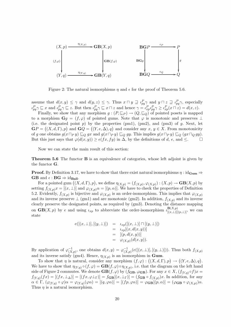
Figure 2: The natural isomorphisms η and ǫ for the proof of Theorem 5.6.

assume that d(x, y) ≤ γ and d(y, z) ≤ γ. Thus x ⊓ y ⊒ ιPpyγ and y ⊓ z ⊒ ιPpyγ, especially

ιPpyγ ⊑ x and ιPpyγ ⊑ z. But then ιPpyγ ⊑ x ⊓ z and hence γ = ιPxpιPpyγ ≥ ιPxp(x ⊓ z) = d(x, z).

Finally, we show that any morphism g : (P,⊑P ) → (Q,⊑Q) of pointed posets is mappedto a morphism Gg = (f, ϕ) of pointed gums. Note that ϕ is monotonic and preserves ⊥(i.e. the designated point p) by the properties (pm1), (pm2), and (pm3) of g. Next, letGP =

(

(X, d,Γ), p)

and GQ =(

(Y, e,∆), q)

and consider any x, y ∈ X. From monotonicityof g one obtains g(x⊓P y) ⊑Q gx and g(x⊓P y) ⊑Q gy. This implies g(x⊓P y) ⊑Q (gx⊓Q gy).But this just says that ϕ(d(x, y)) ≥ e(fx, fy) in ∆, by the definitions of d, e, and ≤. �

Now we can state the main result of this section:

Theorem 5.6 The functor B is an equivalence of categories, whose left adjoint is given bythe functor G.

Proof. By Definition 3.17, we have to show that there exist natural isomorphisms η : idGum ⇒GB and ǫ : BG ⇒ idBall.

For a pointed gum(

(X, d,Γ), p)

, we define η(X,p) = (f(X,p), ϕ(X,p)) : (X, p) → GB(X, p) bysetting f(X,p)x = [(x,⊥)] and ϕ(X,p)α = [(p, α)]. We have to check the properties of Definition5.2. Evidently, f(X,p) is bijective and ϕ(X,p) is an order-isomorphism. This implies that ϕ(X,p)

and its inverse preserve ⊥ (gm1) and are monotonic (gm2). In addition, f(X,p) and its inverseclearly preserve the designated points, as required by (gm3). Denoting the distance mapping

on GB(X, p) by e and using ιxp to abbreviate the order-isomorphism ιB(X,p)[(x,⊥)][(p,⊥)], we can

state

e([(x,⊥)], [(y,⊥)]) = ιxp([(x,⊥)] ⊓ [(y,⊥)])= ιxp[(x, d(x, y))]= [(p, d(x, y))]= ϕ(X,p)(d(x, y)).

By application of ϕ−1(X,p), one obtains d(x, y) = ϕ−1

(X,p)(e([(x,⊥)], [(y,⊥)])). Thus both f(X,p)

and its inverse satisfy (gm4). Hence, η(X,p) is an isomorphism in Gum.To show that η is natural, consider any morphism (f, ϕ) :

(

(X, d,Γ), p)

→(

(Y, e,∆), q)

.We have to show that η(Y,q) ◦ (f, ϕ) = GB(f, ϕ)◦η(X,p), i.e. that the diagram on the left handside of Figure 2 commutes. We denote GB(f, ϕ) by (fGB, ϕGB). For any x ∈ X, (f(Y,q)◦f)x =f(Y,q)(fx) = [(fx,⊥∆)] = [(fx, ϕ⊥Γ)] = fGB[(x,⊥Γ)] = (fGB ◦ f(X,p))x. In addition, for anyα ∈ Γ, (ϕ(Y,q) ◦ ϕ)α = ϕ(Y,q)(ϕα) = [(q, ϕα)] = [(fp, ϕα)] = ϕGB[(p, α)] = (ϕGB ◦ ϕ(X,p))α.Thus η is a natural isomorphism.

20

Next, we define ǫP : BGP → P by ǫP [(x, α)] = ιPx α, for [(x, α)] ∈ BGP . By requirement(P2) of Definition 5.1, the result of this operation is independent of the choice of the repre-sentative x and ǫ is well-defined. Note that the distance ⊥ in GP is just the designated pointp of P and thus all maximal elements of BGP are of the form [(x, p)], x ∈ maxP .

We have to check the properties of Definition 5.3. Elements [(x, p)] ∈ maxBGP aremapped to ιPx (p) ∈ maxP , which is what (pm1) requires. The preservation of designatedpoints (pm3) follows from the fact that ιPp (p) = p.

To show monotonicity (pm2), consider [(x, α)], [(y, β)] ∈ BGP such that [(x, α)] ⊑ [(y, β)].As noted before, this implies that [(x, α)] = [(y, α)]. Hence, using α ≥ β and monotonicity ofιPy , one obtains ιPx α = ιPy α ⊑ ιPy β, with respect to the order of P .

Now for property (pm4), consider [(x, p)] ∈ maxBGP and [(p, α)] ∈ ↓[(p, p)]. Then

ǫP

(

ιBGP[(x,p)][(p, α)]

)

= ǫP [(x, α)]

= ιPx α = ιPǫP [(x,p)]

(

ǫP [(p, α)])

,

where the final equality follows from the facts that x = ιPx p = ǫP [(x, p)] and α = ιPp α =ǫP [(p, α)].

To see that ǫP is an isomorphism, consider an element a ∈ P . We define κP (a) = [(x, ιPxpa)],for any x ∈ maxP with a ⊑ x. Property (P1) of Definition 5.1 implies that such an x exists.Assume there is another element y ∈ maxP with a ⊑ y. Property (P2) implies ιPxpa = ιPypa.Since d(x, y) in GP is defined to be isomorphic to the greatest lower bound x ⊓ y in P ,ιPxpa ⊑ d(x, y) and therefore ιPxpa ≥ d(x, y). Hence we deduce that [(x, ιPxpa)] = [(y, ιPypa)] andthat κ is well-defined.

Furthermore, ǫ and κ are inverse to each other, since ǫPκPa = ǫP [(x, ιPxpa)] = ιPx ιPxpa = a

and κP ǫP [(x, α)] = κP ιPx α = [(x, ιPxpι

Px α)] = [(x, α)].

We also have to check the properties (pm1) to (pm4) for κ. As before, it is easy to seethat (pm1) and (pm3) hold. Property (pm2) follows from monotonicity of ǫ and the fact thatκ is its inverse. For (pm4), let x ∈ maxP and a ∈ ↓p. Using the abbreviation θ = κP , we find

θ(ιPx a) = [(x, ιPxpιPx a)] = [(x, a)]

= ιBGP[(x,p)][(p, a)] = ιBGP

θ(x) (θa),

where the final equality follows from [(x, p)] = ιPxp[(x, x)] = θx and [(p, a)] = ιPpp[(p, a)] = θa.Naturality of ǫ is again shown via a straightforward calculation (compare the right diagram

of Figure 2). Consider some morphism g : P → Q and let [(x, α)] ∈ BGP . Then (g ◦ǫP )[(x, α)] = g(ιPx α) = ιQ

g(x)gα = ǫQ[(gx, gα)] = (ǫQ ◦BGg)[(x, α)]. This finishes the proof. �

In the rest of this section, we consider various subcategories of Gum and Ball. Gumdcpo∗

is the full subcategory of Gum consisting of pointed gums (X, d,Γ), where X is chain-spherically complete and Γ∂ is a dcpo. The subcategory of Gumdcpo∗ obtained by restrictingto morphisms (f, ϕ) for which ϕ is Scott-continuous will be called Gumdcpo. Note thatScott-continuity refers to the dual orders of distances by the definition of ϕ. To see that thisis indeed a subcategory, one just has to check that the composition law of Gum preservesthis additional property.

The complementing categories of pointed posets are denoted Balldcpo∗ and Balldcpo.Balldcpo∗ is the full subcategory consisting just of directed complete pointed posets, calledpointed dcpos, and Balldcpo is the subcategory of Balldcpo∗ where the morphisms additionallyare Scott-continuous.

21

Theorem 5.7 The functors B and G restrict to an equivalence of the categories Gumdcpo∗

(Gumdcpo) and Balldcpo∗ (Balldcpo).

Proof. By Corollary 4.4, it is clear that objects from Gumdcpo∗ are indeed mapped toBalldcpo∗. For the converse, consider a pointed dcpo (P, p). By Theorem 5.6, BG(P, p) isisomorphic to (P, p). But this implies that BG(P, p) is a pointed dcpo and we can again useCorollary 4.4 to show that G(P, p) is an object of Gumdcpo∗. This already shows that thefunctors B and G restrict to the categories Gumdcpo∗ and Balldcpo∗. For Gumdcpo andBalldcpo we still have to consider morphisms.

We show that morphisms of Gumdcpo are mapped to morphisms of Balldcpo, i.e. thatthe additional requirement of Scott-continuity is satisfied. Consider a morphism g = B(f, ϕ),where (f, ϕ) : (X, p) → (Y, q) is a morphism of Gumdcpo, and a directed subset A ⊆ BX with⊔

A = [(x, α)]. For any [(y, β)] ∈ A, g[(y, β)] ⊑BY g[(x, α)], i.e. g[(x, α)] is an upper bound ofg(A). By Corollary 4.2, α is the least upper bound of the directed set Λ = {β | [(y, β)] ∈ A}within Γ∂ , the dual poset of distances of X. Scott-continuity of ϕ with respect to Γ∂ yieldsthat

∨∂ ϕ(Λ) = ϕ(α). Thus g[(x, α)] is the least upper bound of g(A), again by Corollary 4.2.To see that a morphism g of Balldcpo is also mapped to a morphism of Gumdcpo, just

note that the mapping ϕ in Gg = (f, ϕ) simply is the restriction of g to ↓p and consequentlyinherits Scott-continuity. Therefore the functors B and G restrict to the categories Gumdcpo

and Balldcpo.The claimed equivalence of categories now follows from the proof of Theorem 5.6 together

with the observation that the required natural isomorphisms are just the restrictions of theabove definitions of η and ǫ to the respective subcategories. To see that these restrictions arealso morphisms in Gumdcpo and Balldcpo, one just has to note that order-isomorphisms arealways Scott-continuous. �

It is easy to see that similar results could be shown for categories that impose furtherrestrictions on the objects. Especially, Theorem 4.17 suggests that one could include (ω-)continuity as well. Proving that B and G restrict to these classes of objects is done by acompletely similar reasoning as in the first part of the above proof. For the class of morphismsone can freely choose whether Scott-continuity should be required or not. In any case, noadditional verifications are needed to establish the desired categorical equivalences.

6 Fixed point theorems

In the following, we give a domain theoretic proof for a variant of the Prieß-Crampe and Riben-boim theorem (see [16]), where we restrict ourselves to gums from the category Gumdcpo∗.For more special situations, we can even prove a theorem that can be compared with the Ba-nach fixed point theorem, in the sense that it obtains the desired fixed point from a countablechain of closed balls. Since we do not need all of the categorical results from the previous sec-tion here, we will give the necessary preconditions explicitly, dropping some of the structurethat was introduced for Gum. The proof follows the ones of [5, Theorem 18] and [12, p.16].

Theorem 6.1 Let (X, d,Γ) be a gum, where Γ∂ is a dcpo andX is chain-spherically complete.Consider mappings f : X → X and ϕ : Γ∂ → Γ∂ , such that, for all α ∈ Γ\{⊥}, ϕα < α and,for all x, y ∈ X, d(fx, fy) ≤ ϕ(d(x, y)). Then the following hold:

(i) If ϕ is monotonic, then f has a unique fixed point on X.

22

(ii) If ϕ is Scott-continuous, then the unique fixed point of f is the only element of thesingleton set

⋂

n∈NBϕnd(x,fx)(f

nx), for arbitrary x ∈ X.

Proof. Although we ignore some of the categorical structure introduced above, we can stilldefine B(f, ϕ) as before.

We want to find an arbitrary fixed point of B(f, ϕ) on BX. Consider some point x ∈ Xand set α = d(x, fx). Assume without loss of generality that x is not a fixed point of f . Forall [(y, β)] ⊒ [(x, α)], we have ϕβ < β ≤ α and d(fx, fy) ≤ ϕ(d(x, y)) < d(x, y) ≤ α. Usingthe strong triangle inequality on d(x, fx) = α and d(fx, fy) ≤ α, one gets d(x, fy) ≤ α andconsequently [(fy, ϕβ)] ⊒ [(x, α)]. Thus B(f, ϕ) maps ↑[(x, α)] to itself.

Since ↑[(x, α)] by Corollary 4.4 is a cpo with least element [(x, α)], we can apply the fixedpoint theorems stated in Section 3. Note that B(f, ϕ) is monotonic, as shown in Proposition5.4. Thus, by Proposition 3.9, B(f, ϕ) has a (least) fixed point [(z, γ)] on ↑[(x, α)]. Further-more, if ϕ is Scott-continuous, Theorem 5.7 asserts that B(f, ϕ) is also Scott-continuous and

hence [(z, γ)] =⊔↑

n∈N[(fnx, ϕnα)] by Proposition 3.8.

Now B(f, ϕ)[(z, γ)] = [(z, γ)] implies that ϕγ = γ and thus γ = ⊥. However, formal ballsof the form [(z,⊥)] are equivalence classes with only one representative and thus fz = z, i.e.z is a fixed point of f . To show the uniqueness of z, suppose for a contradiction that there isz′ 6= z such that fz′ = z′. Then d(z, z′) = d(fz, fz′) ≤ ϕ(d(z, z′)) < d(z, z′).

For the Scott-continuous case, we already observed that [(fnx, ϕnα)]n∈N is a chain in BX.By the definition of ⊑,

(

Bϕnα(fnx))

n∈Nis a chain of closed balls with z ∈

⋂

n∈NBϕnα(fnx).

To see that this intersection is indeed a singleton set, assume that there is a z′ 6= z such thatz′ ∈

⋂

n∈NBϕnα(fnx). Then d(fnx, z′) ≤ ϕnα for every n ∈ N and hence [(z′, 0)] is an upper

bound of [(fnx, ϕnα)]n∈N. This contradicts the assumption that [(z, 0)] is the least such upperbound. �

We can compare part (i) of this theorem with [16, 5.3 (2)]. It is clear that our preconditionsare strictly stronger than those required in [16]3, although the obtained result is not. Thisdeserves some discussion.

First of all, we have to verify that the preconditions are indeed stronger than those inthe original theorem. Instead of assuming that d(fx, fy) < d(x, y), i.e. that f is strictlycontracting, we require the existence of a mapping ϕ that gives a uniform bound for thecontraction of f . As the following example will show, this is a strictly stronger assumption.

Example 6.2 This example will again be a variation of the classical ultrametric of infinitewords. We use the notation of Example 4.18. Let X = {a, b}ω be a set of points and define aset of distances by Γ = {0, 1, ω} ∪

(

{n ∈ N | n >N 1} × {a, b})

. Hence Γ consists of two copiesof N ∪ {ω}, where 0, 1, and ω are identified. We define the order ≤ on Γ by setting x < y iffone of the following holds:

(i) x = ω and y 6= ω,

(ii) x 6= 0 and y = 0,

(iii) x 6= 0, x 6= 1 and y = 1,

(iv) x = (n, l) and y = (m, l), for n, m ∈ N and l ∈ {a, b}, where n > m.

3Strictly speaking, our condition of X being chain-spherically complete is weaker than the requirement ofspherical completeness in [16]. However, their proof can be modified to use the weaker assumption as well.

23

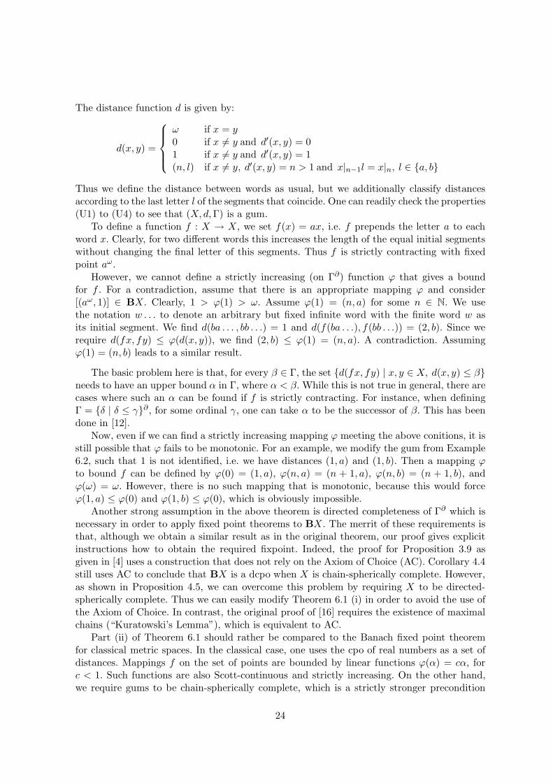
The distance function d is given by:

d(x, y) =

ω if x = y0 if x 6= y and d′(x, y) = 01 if x 6= y and d′(x, y) = 1(n, l) if x 6= y, d′(x, y) = n > 1 and x|n−1l = x|n, l ∈ {a, b}

Thus we define the distance between words as usual, but we additionally classify distancesaccording to the last letter l of the segments that coincide. One can readily check the properties(U1) to (U4) to see that (X, d,Γ) is a gum.

To define a function f : X → X, we set f(x) = ax, i.e. f prepends the letter a to eachword x. Clearly, for two different words this increases the length of the equal initial segmentswithout changing the final letter of this segments. Thus f is strictly contracting with fixedpoint aω.

However, we cannot define a strictly increasing (on Γ∂) function ϕ that gives a boundfor f . For a contradiction, assume that there is an appropriate mapping ϕ and consider[(aω, 1)] ∈ BX. Clearly, 1 > ϕ(1) > ω. Assume ϕ(1) = (n, a) for some n ∈ N. We usethe notation w . . . to denote an arbitrary but fixed infinite word with the finite word w asits initial segment. We find d(ba . . . , bb . . .) = 1 and d(f(ba . . .), f(bb . . .)) = (2, b). Since werequire d(fx, fy) ≤ ϕ(d(x, y)), we find (2, b) ≤ ϕ(1) = (n, a). A contradiction. Assumingϕ(1) = (n, b) leads to a similar result.

The basic problem here is that, for every β ∈ Γ, the set {d(fx, fy) | x, y ∈ X, d(x, y) ≤ β}needs to have an upper bound α in Γ, where α < β. While this is not true in general, there arecases where such an α can be found if f is strictly contracting. For instance, when definingΓ = {δ | δ ≤ γ}∂ , for some ordinal γ, one can take α to be the successor of β. This has beendone in [12].

Now, even if we can find a strictly increasing mapping ϕ meeting the above conitions, it isstill possible that ϕ fails to be monotonic. For an example, we modify the gum from Example6.2, such that 1 is not identified, i.e. we have distances (1, a) and (1, b). Then a mapping ϕto bound f can be defined by ϕ(0) = (1, a), ϕ(n, a) = (n + 1, a), ϕ(n, b) = (n + 1, b), andϕ(ω) = ω. However, there is no such mapping that is monotonic, because this would forceϕ(1, a) ≤ ϕ(0) and ϕ(1, b) ≤ ϕ(0), which is obviously impossible.

Another strong assumption in the above theorem is directed completeness of Γ∂ which isnecessary in order to apply fixed point theorems to BX. The merrit of these requirements isthat, although we obtain a similar result as in the original theorem, our proof gives explicitinstructions how to obtain the required fixpoint. Indeed, the proof for Proposition 3.9 asgiven in [4] uses a construction that does not rely on the Axiom of Choice (AC). Corollary 4.4still uses AC to conclude that BX is a dcpo when X is chain-spherically complete. However,as shown in Proposition 4.5, we can overcome this problem by requiring X to be directed-spherically complete. Thus we can easily modify Theorem 6.1 (i) in order to avoid the use ofthe Axiom of Choice. In contrast, the original proof of [16] requires the existence of maximalchains (“Kuratowski’s Lemma”), which is equivalent to AC.

Part (ii) of Theorem 6.1 should rather be compared to the Banach fixed point theoremfor classical metric spaces. In the classical case, one uses the cpo of real numbers as a set ofdistances. Mappings f on the set of points are bounded by linear functions ϕ(α) = cα, forc < 1. Such functions are also Scott-continuous and strictly increasing. On the other hand,we require gums to be chain-spherically complete, which is a strictly stronger precondition

24

than the completeness needed in the classical setting (for details, we refer to [8, Section 1.3]).Another additional constraint is of course the strong triangle inequality, which one cannotavoid when dealing with arbitrary posets of distances. Finally, we remark that we do notneed AC here either. In fact, since we consider only the supremum of a chain, the proof of theemployed fixed point theorem (Proposition 3.8) remains valid as long as chains have a leastupper bound in BX. For this it suffices to assume that X is chain-spherically complete, asdemonstrated in Proposition 4.3.

Summing up, one may argue that, in order to find a result as strong as Theorem 6.1(ii), one needs to keep up many strong restrictions known from classical metric spaces. Theadditional requirements on (spherical) completeness and the triangle inequality account forthe broader class of possible distance sets one obtains when considering gums.

7 Summary and conlcusion

Taking up a technique from [5] that was suggested for the study of generalized ultrametricspaces in [12], we have investigated the relation between gums and their spaces of formalballs. In Section 4, it was shown that there are close connections between domain theoreticproperties of the space of formal balls BX and the dually ordered set of distances of a gum Γ∂ .Especially, certain completeness conditions on the ultrametric and its set of distances werefound to have equivalent completeness properties for BX. In addition, the metric topologyof a gum was studied and conditions were introduced for which the domain BX yields acomputational model for this topology. It was argued that similar restrictions should beimposed on the very general notion of a gum in order to obtain a reasonably well-behavedmetric topology. After all, it remains an open question, in which way a topology on a gumshould be defined. Our results give evidence that various possible definitions may coincidewhen using appropriate conditions.

In Section 5, the connections between a gum and its space of formal balls were studied inthe setting of category theory. For this purpose, appropriate categories of gums and of partialorders were introduced and the functor B was extended to the morphisms of these categories.By demonstrating that B is indeed the left adjoint of a categorical equivalence, it could beshown that the spaces of formal balls actually form a very restricted subcategory of all posets.This observation raises doubts concerning the use of B as a tool for establishing a connectionbetween the theory of ultrametric spaces and domain theory.

Yet, in Section 6, the space of formal balls could be employed to obtain a modified versionof the Prieß-Crampe and Ribenboim Theorem, which establishes the original result withoutthe use of the Axiom of Choice. However, the possibility to describe the required fixed pointinstead of just stating its mere existence comes at the price of stronger preconditions. Afurther strengthening of the assumptions even led to a result that may be compared to theBanach fixed point theorem for classical metric spaces, since a fixed point is described as theintersection of an ω-chain of closed balls.

From our considerations, one may draw various conclusions concerning the study of thespace of formal balls and of generalized ultrametric spaces. First of all, the rather peculiarcharacteristics of the category of formal balls suggests that this approach is not appropriateto link gums to the area of domain theory. Still this result settles the conjecture that thismethod could be used for this purpose. One might also presume that a similar characterizationis possible in the classical case as well. Furthermore, it has been shown that the space of formal

25

balls can effectively contribute to investigate properties of gums. In fact, it played a vital rolein the investigation of the metric topology as well as in the validation of two fixed pointtheorems. Finally, the treatment of gums in their full generality lead to the discovery ofvarious special conditions on the set of distances, which gave accurate characterizations ofcertain desired situations. In the light of these findings, stronger restrictions, such as linearityor directedness of the distance set, might be relaxed in future works on this topic.

Acknowledgement. I am most grateful for the continuous support and motivation fromDr. Pascal Hitzler without whom this work would probably never have been finished andsurely would not have been started. Patiently checking numerous preliminary versions of thispaper and providing me with valuable comments, he contributed much to the enhancementof both clarity and correctness of this presentation.

References

[1] S. Abramsky and A. Jung. Domain theory. In S. Abramsky, D. M. Gabbay, and T. S. E.Maibaum, editors, Handbook of Logic in Computer Science, volume III. Oxford UniversityPress, 1994.

[2] F. Borceux. Handbook of Categorical Algebra 1: Basic Category Theory, volume 53 ofEncyclopedia of Mathematics and its Applications. Cambridge University Press, 1994.

[3] M. M. Bosangue, F. van Breugel, and J. J. M. M. Rutten. Generalized metric spaces:Completion, topology, and powerdomains via the Yoneda embedding. Theoretical Com-puter Science, 193:1–51, 1998.

[4] B. A. Davey and H. A. Priestley. Introduction to Lattices and Order. Cambridge Uni-versity Press, second edition, 2002.

[5] A. Edalat and R. Heckmann. A computational model for metric spaces. TheoreticalComputer Science, 193:53–73, 1998.

[6] R. C. Flagg. Quantales and continuity spaces. Algebra Universalis, 37(3):257–276, 1997.

[7] G. Gierz, K. H. Hofmann, K. Keimel, J. D. Lawson, M. Mislove, and D. S. Scott. Con-tinuous Lattices and Domains, volume 93 of Encyclopedia of Mathematics and its Appli-cations. Cambridge University Press, 2003.

[8] P. Hitzler. Generalized Metrics and Topology in Logic Programming Semantics. PhDthesis, Department of Mathematics, National University of Ireland, University CollegeCork, 2001.

[9] P. Hitzler and A. K. Seda. Acceptable programs revisited. In Proceedings of the Work-shop on Verification in Logic Programming, 16th International Conference on Logic Pro-gramming (ICLP’99), volume 30 of Electronic Notes in Theoretical Computer Science.Elsevier, Amsterdam, 1999.

[10] P. Hitzler and A. K. Seda. A new fixed point theorem for logic programming semantics.In Proceedings of the joint IIIS & IEEE meeting of the 4th World Multiconference on Sys-temics, Cybernetics and Informatics (SCI2000) and the 6th International Conference on

26

Information Systems Analysis and Synthesis (ISAS2000), 2000, volume VII, ComputerScience and Engineering Part 1, pages 418–423. International Institute of Informaticsand Systemics, 2000.

[11] P. Hitzler and A. K. Seda. The fixed-point theorems of Priess-Crampe and Ribenboimin logic programming. In Valuation Theory and its Applications, Proceedings of the1999 Valuation Theory Conference, University of Saskatchewan in Saskatoon, Canada,volume 32 of Fields Institute Communications, pages 219–235. American MathematicalSociety, 2002.

[12] P. Hitzler and A. K. Seda. Generalized metrics and uniquely determined logic programs.Theoretical Computer Science, 305(1–3):187–219, 2003.

[13] R. Kopperman. All topologies come from generalized metrics. American MathematicalMonthly, 95(2):89–97, 1988.

[14] S. G. Matthews. Partial metric toplogy. In Proceedings of the 8th Summer Conference onGeneral Topology and its Applications, volume 728 of Annals of the New York Academyof Sciences, pages 183–197, 1994.

[15] S. J. O’Neill. A Fundamental Study into the Theory and Application of the Partial MetricSpaces. PhD thesis, Department od Computer Science, University of Warwick, 1998.

[16] S. Prieß-Crampe and P. Ribenboim. Logic programming and ultrametric spaces. Rendi-conti di Mathematica, VII(19):155–176, 1999.

[17] J. J. M. M. Rutten. Weighted colimits and formal balls in generalized metric spaces.Technical Report SEN–R9711, CWI, Amsterdam, 1997.

[18] M. P. Schellekens. A charachterization of partial metrizability. domains are quantifiable.Theoretical Computer Science, 305:409–432, 2003.

[19] M. B. Smyth. Reconciling domains and metric spaces. In M. Main, A. Melton, M. Mislove,and D. Schmidt, editors, Proceedings of the Workshop on Mathematical Foundations ofProgramming Language Semantics, number 298 in Lecture Notes in Computer Science,pages 236–253. Springer, 1988.

[20] M. B. Smyth. Topology. In S. Abramsky, D. M. Gabbay, and T. S. E. Maibaum, editors,Handbook of Logic in Computer Science, volume I. Oxford University Press, 1992.

[21] P. Waszkiewicz. Quantitative Continuous Domains. PhD thesis, School of ComputerScience, University of Birmingham, 2002.

27