GENERALIZED STIRLING NUMBERS,

CONVOLUTION FORMULAE AND p, q-ANALOGUES

Anne de Medicis*

Pierre Leroux†

School of Mathematics,University of Minnesota, Minneapolis

LACIM,Universite du Quebec a Montreal

Abstract. In this paper, we study two generalizations of the Stirling numbers of thefirst and second kinds, inspired from their combinatorial interpretation in terms of0–1 tableaux. They are the A-Stirling numbers and the partial Stirling numbers. In

particular, we give a q and a p, q-analogue of convolution formulae for Stirling num-bers of the second kind, due to Chen and Verde-Star, and we extend these formulaeto Stirling numbers of the first kind. Included in this study are the a, d-progressive

Stirling numbers, corresponding to 0–1 tableaux with column lengths from an arith-metic progression {a + id}i≥0.

Resume. Dans cet article, nous etudions deux generalisations des nombres de Stir-ling de premiere et deuxieme especes, inspirees par leur interpretation combinatoireen termes de tableaux 0–1. Il s’agit des A-nombres de Stirling et des nombres de

Stirling partiels. Nous donnons en particulier des q et p, q-analogues de formules deconvolution des nombres de Stirling de deuxieme espece, dues a Chen et Verde-Star,et nous etendons ces formules aux nombres de Stirling de premiere espece. Les nom-

bres de Stirling a, d-progressifs, correspondant aux tableaux 0–1 dont les longueursdes colonnes font partie d’une progression arithmetique {a + id}i≥0, sont egalementinclus dans cette etude.

1 INTRODUCTION

A 0–1 tableau is a pair ϕ = (λ, f), where λ = (λ1 ≥ λ2 ≥ . . . ≥ λk) is apartition of an integer m = |λ|, and f = (fij)1≤j≤λi is a “filling” of the cells ofthe corresponding Ferrers diagram of shape λ with 0’s and 1’s, such that there isexactly one 1 in each column.

1991 Mathematics Subject Classification. Primary: 05A15; Secondary: 11B65, 11B73..*This work was supported by NSERC (Canada) and FCAR (Quebec) Scholarships.†This work was supported by NSERC (Canada) and FCAR (Quebec).

Typeset by AMS-TEX

1

0 0 0 0 1 0 1 1

1 0 1 0 0 0 0

0 1 0 1 0 1

0 0

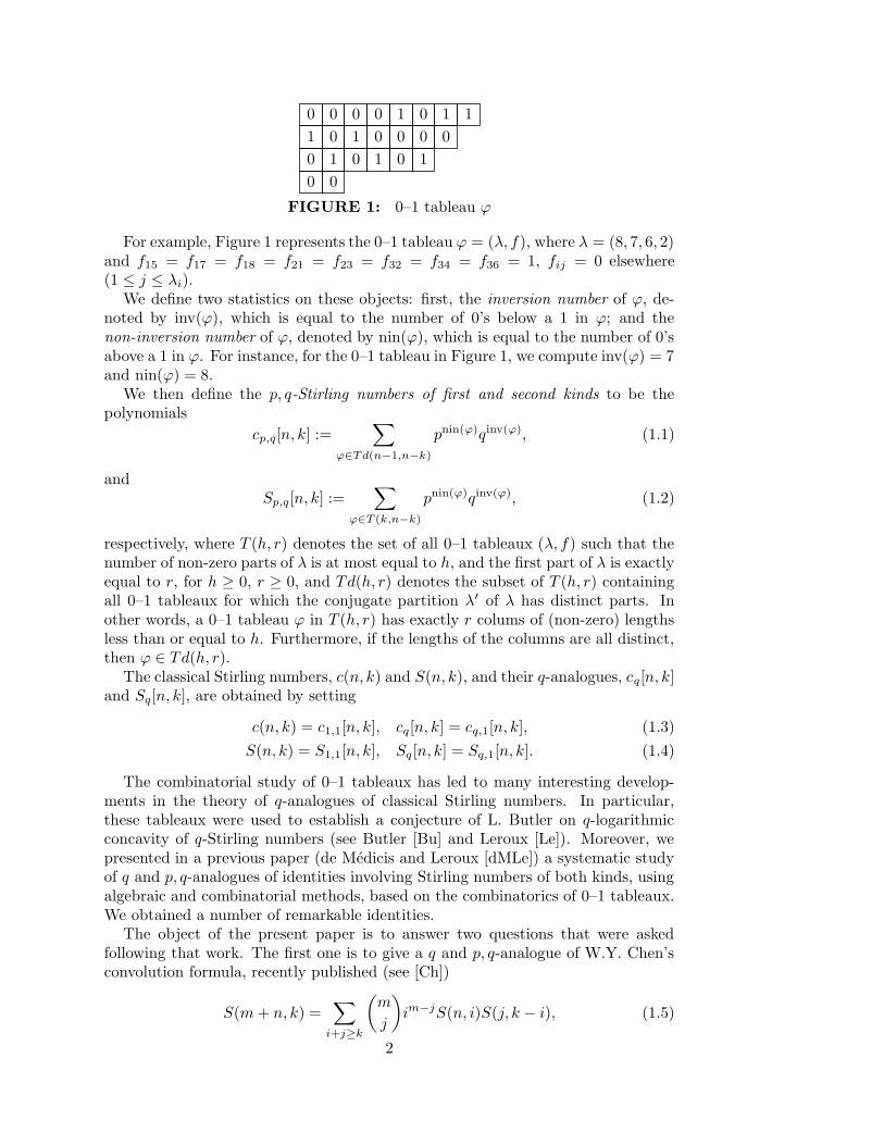
FIGURE 1: 0–1 tableau ϕ

For example, Figure 1 represents the 0–1 tableau ϕ = (λ, f), where λ = (8, 7, 6, 2)and f15 = f17 = f18 = f21 = f23 = f32 = f34 = f36 = 1, fij = 0 elsewhere(1 ≤ j ≤ λi).

We define two statistics on these objects: first, the inversion number of ϕ, de-noted by inv(ϕ), which is equal to the number of 0’s below a 1 in ϕ; and thenon-inversion number of ϕ, denoted by nin(ϕ), which is equal to the number of 0’sabove a 1 in ϕ. For instance, for the 0–1 tableau in Figure 1, we compute inv(ϕ) = 7and nin(ϕ) = 8.

We then define the p, q-Stirling numbers of first and second kinds to be thepolynomials

cp,q[n, k] :=∑

ϕ∈Td(n−1,n−k)

pnin(ϕ)qinv(ϕ), (1.1)

andSp,q[n, k] :=

∑

ϕ∈T (k,n−k)

pnin(ϕ)qinv(ϕ), (1.2)

respectively, where T (h, r) denotes the set of all 0–1 tableaux (λ, f) such that thenumber of non-zero parts of λ is at most equal to h, and the first part of λ is exactlyequal to r, for h ≥ 0, r ≥ 0, and Td(h, r) denotes the subset of T (h, r) containingall 0–1 tableaux for which the conjugate partition λ′ of λ has distinct parts. Inother words, a 0–1 tableau ϕ in T (h, r) has exactly r colums of (non-zero) lengthsless than or equal to h. Furthermore, if the lengths of the columns are all distinct,then ϕ ∈ Td(h, r).

The classical Stirling numbers, c(n, k) and S(n, k), and their q-analogues, cq[n, k]and Sq[n, k], are obtained by setting

c(n, k) = c1,1[n, k], cq[n, k] = cq,1[n, k], (1.3)

S(n, k) = S1,1[n, k], Sq [n, k] = Sq,1[n, k]. (1.4)

The combinatorial study of 0–1 tableaux has led to many interesting develop-ments in the theory of q-analogues of classical Stirling numbers. In particular,these tableaux were used to establish a conjecture of L. Butler on q-logarithmicconcavity of q-Stirling numbers (see Butler [Bu] and Leroux [Le]). Moreover, wepresented in a previous paper (de Medicis and Leroux [dMLe]) a systematic studyof q and p, q-analogues of identities involving Stirling numbers of both kinds, usingalgebraic and combinatorial methods, based on the combinatorics of 0–1 tableaux.We obtained a number of remarkable identities.

The object of the present paper is to answer two questions that were askedfollowing that work. The first one is to give a q and p, q-analogue of W.Y. Chen’sconvolution formula, recently published (see [Ch])

S(m+ n, k) =∑

i+j≥k

(

m

j

)

im−jS(n, i)S(j, k − i), (1.5)

2

and to also find a similar formula for Stirling numbers of the first kind. The secondquestion that was raised is to determine which properties remain valid when someconstraints are imposed on the lengths of the columns in 0–1 tableaux, such asrequiring lengths to be part of an arithmetic or a geometric progression.

In view of these problems, we consider two natural generalizations of Stirlingnumbers in the context of 0–1 tableaux, the A-Stirling numbers and the partialStirling numbers.

The A-Stirling numbers are obtained by restricting the possible choices of lengthsof columns and also by replacing the p, q-counting of fillings of columns by someweight on the columns. More precisely, let A = (A, w), where A = (ai)i≥0 denotes

a strictly increasing sequence of non-negative integers (the column lengths allowed),and w : N → K denotes a function from N to a ring K (column weights accordingto length). We define an A-tableau to be a list φ of columns c of a Ferrers diagramof a partition λ (by decreasing order of length) such that the lengths |c| are part ofthe sequence A, and we set

wA(φ) =∏

c∈φ

w(|c|). (1.6)

Note that φ might contain a finite number of columns of length zero if 0 is part ofthe sequence A and if w(0) 6= 0. We then define the A-Stirling numbers of the firstkind (without sign) and of the second kind to be respectively

cA(n, k) :=∑

φ∈TdA(n−1,n−k)

wA(φ), (1.7)

and

SA(n, k) :=∑

φ∈TA(k,n−k)

wA(φ), (1.8)

where TA(h, r) denotes the set of A-tableaux with exactly r columns whose lengths

are in the set {a0, a1, . . . , ah}, and TdA(h, r) denotes the subset of TA(h, r) con-taining all A-tableaux with columns of distinct lengths.

As for the p, q-Stirling numbers, by considering the maximum possible length ofcolumns of A-tableaux and their format, we get the following recurrences, wherewe set wi = w(ai):

cA(n, k) = cA(n− 1, k − 1) + wn−1cA(n− 1, k), (1.9)

and

SA(n, k) = SA(n− 1, k − 1) + wkSA(n− 1, k), (1.10)

with initial boundary conditions cA(0, k) = δ0,k = SA(0, k), cA(n, 0) = w0w1 . . . wn−1

and SA(n, 0) = wn0 .Similar generalizations of Stirling numbers can be found in the literature. We

are thus extending, from a combinatorial point of view, previous works such asthose of L. Comtet [Co], M. Koutras [Ko], B. Voigt [Vo] and L. Verde-Star [VS].

3

Many classical families of numbers or polynomials arise as particular cases ofA-Stirling numbers. Table 1 gives an outlook of some of the families that occurin combinatorics. In section 2, we display the main properties shared by all ofthese families, as well as some connections that might occur between two relatedfamilies, such as when a weight function w∗ is obtained by multiplying anotherweight function w by a constant, w∗(x) = a · w(x), or is obtained by adding aconstant, w∗(x) = a + w(x), or still yet when the length sequence is obtained bytranslation δmA of a given sequence A. It is in this context that the convolutionformulae extending Chen’s formula (1.5) will be stated in the greatest generality(see Theorem 2.6, and also [VS], Proposition 5.4 and 5.5).

TABLE 1

wi SA(n, k) References cA(n, k)

1 1(

nk

)

binomial coefficients(

nk

)

2 i S(n, k) Stirling numbers c(n, k)

3 i2 T (2n, 2k) [Ri] (Riordan) pp. 212–249 (−1)n−kt(2n, 2k)

4 (2i)2 Simp(2n, 2k) partitions with odd

blocks [Co]

5 (2i+ 1)2 Simp(2n+ 1, 2k + 1) partitions with odd

blocks [Co]

6 qi[

nk

]

qq-binomial coefficients q(

n−k2 )[n

k

]

q

7 qi+1 qn−k[

nk

]

qaffine subspaces q(

n−k+1

2 )[nk

]

q

8 [i]p,q Sp,q[n, k] p,q-Stirling numbers cp,q[n, k]

9 qi − 1 (q − 1)n−kSq [n, k] q-tableaux with no (q − 1)n−kcq[n, k]null columns, Section 2

10 a+ i∑

m

(

nm

)

an−mS(m,k) Section 4∑

m

(

mk

)

am−kc(n,m)

11 −a+ i S(a)(n, k) non-central Stirling c(a)(n, k)numbers [Ko], Section 2

12 1 + iα WG(n, k) Whitney numbers of (−1)n−kwG(n, k)Dowling lattices [Do]

13 [a+ id]p,q Sa,dp,q [n, k] a,d-progressive Stirling ca,dp,q [n, k]numbers, Section 4

The second generalization, partial Stirling numbers, is adressed in Section 3.It is obtained by considering weak 0–1 tableaux, i.e. 0–1 tableaux that are weakin the sense that some columns may contain only 0’s, contributing to the non-inversion statistic. They correspond, in the traditional combinatorial interpreta-tions, to partial partitions and to permutations with some marked cycles. Thepartial p, q-Stirling numbers Pcp,q[n,m, k] and PSp,q[n,m, k] are defined by p, q-counting weak 0–1 tableaux with a fixed number of columns filled with 0’s. Whenthe number of columns filled with 0’s is not fixed, the corresponding polynomialfamilies, Pcp,q[n, k] =

∑

mPcp,q[n,m, k] and PSp,q[n, k] =∑

m PSp,q[n,m, k] forma particular case of A-Stirling numbers, with ai = i and w(i) = pi + [i]p,q .

In Section 3, we extend to weak 0–1 tableaux the natural bijections between4

0–1 tableaux and partitions or permutations (see de Medicis and Leroux [dMLe]).We then present a study of identities involving partial p, q-Stirling numbers. Themain point in this section is the resolution of the first problem mentioned above,finding p, q-analogues and extensions of the convolution formula (1.5) (see Propo-sition 3.10). The specialization p = 1 leads to the following convolution formulaefor q-Stirling numbers:

cq[m+ n, k] =∑

i+j≥k

{

(

m+ k − i− j

k − i

)

qn(i+j−k)[n]m−jq

cq[n, i]cq [m,m + k − i− j]

}

, (1.11)

Sq[m+ n, k] =∑

i+j≥k

(

m

j

)

qi(i+j−k)[i]m−jq Sq [n, i]Sq [j, k − i]; (1.12)

cq[n+ 1, k + l + 1] =n

∑

i=0

n−l−i∑

j=0

{

(

l + j

j

)

q(i+1)(n−l−i−j)[i+ 1]jq

cq[i, k]cq [n− i, l + j]

}

, (1.13)

and

Sq[n+ 1, k + l + 1] =n

∑

i=0

n−l−i∑

j=0

{

(

n− i

j

)

q(k+1)(n−l−i−j)[k + 1]jq

Sq [i, k]Sq [n− i− j, l]

}

. (1.14)

The model of weak 0–1 tableaux also appears in the analysis of a, d-progressivep, q-Stirling numbers ca,dp,q [n, k] and Sa,dp,q [n, k], introduced in the last section. Theyare particular cases of A-Stirling numbers where the ai form an arithmetic progres-sion ai = a+ id, a, d ∈ N, and where w(x) = [x]p,q.

Many interesting cases (e.g. items 1, 2, 8, 10 to 13 of Table 1) are covered bythese polynomials. Here we deduce, from the combinatorial models, properties thatare valid in general, in particular the p, q-analogues and extensions of convolutionformulae due to L. Verde-Star (see Proposition 4.5). For p = q = 1, the a, d-progressive Stirling numbers were also studied by J.B. Remmel and M. Wachs[ReWa] and by A. Rucinski and B. Voigt [RuVo], who showed that if a+d > 0, the

numbers Sa,d1,1 (n, k) satisfy a local limit theorem.

2. GENERAL STUDY OF A-STIRLING NUMBERS

In this section, we present the basic properties of A-Stirling numbers and some re-sults linking two related families A and A

∗. The first proposition contains the mostelementary results generalizing properties of p, q-Stirling numbers (see de Medicis

5

and Leroux [dMLe]). These identities can be proven similarly to those in [dMLe],using either the combinatorics of A-tableaux (bijectively or by applying an involu-tion), or algebraically. Details are left to the reader.

PROPOSITION 2.1: Let(

cA(n, k))

n,kand

(

SA(n, k))

n,kbe the families of

polynomials defined by the recurrence relations (1.9) and (1.10). Then the followingidentities hold:

a) (symmetric functions)

cA(n, k) = en−k(w0, w1, w2, . . . , wn−1) (2.1)

=∑

0≤i1<...<in−k≤n−1

wi1 . . . win−k , [Co,(12)]

SA(n, k) = hn−k(w0, w1, w2, . . . , wk) (2.2)

=∑

0≤i1≤...≤in−k≤k

wi1 . . . win−k , [Co,(10)]

where en(x1, x2, . . . , xk) and hn(x1, x2, . . . , xk) denote respectively the elemen-tary and complete symmetric functions of degree n in k variables;

b) (generating functions)For n ≥ 0,

∑

r≥0

cA(n, r)yn−rxr =(

x+ w0y)(

x+ w1y)

. . .(

x+ wn−1y)

, (2.3)

[Co,(1)]

for k ≥ 0,

∑

r≥0

SA(k + r, k)xr =1

(

1− w0x)

1(

1− w1x) . . .

1(

1− wkx) , (2.4)

[Co,(8)]

xn =n

∑

k=0

SA(n, k)(x− w0)(x− w1) . . . (x− wk−1); (2.5)

[Co,(2)]

c) (recurrence relations)

cA(n+ 1, k + 1) =

n∑

j=k

wnwn−1 . . . wj+1cA(j, k), (2.6)

[Co,(7)]

SA(n+ 1, k + 1) =n

∑

j=k

wn−jk+1S

A(j, k), (2.7)

[Co,(6)]6

cA(n, k) =n

∑

j=k

(−1)j−kwj−kn cA(n+ 1, j + 1), (2.8)

[Co,(5)]

SA(n, k) =n−k∑

j=0

(−1)jwk+1wk+2 . . . wk+jSA(n+ 1, k + j + 1); (2.9)

d) (orthogonality relations)

n∑

k=m

sA(n, k)SA(k,m) = δn,m, (2.10)

n∑

k=m

SA(n, k)sA(k,m) = δn,m, (2.11)

where sA(n, k) = (−1)n−kcA(n, k) are the A-Stirling numbers of the first kindwith signs;

e) (other identities)Let ξjA be the sequence obtained from A = (ai)i≥0 by erasing the term aj , andlet ξjA = (ξjA, w). Then

(n− k)cA(n, k) =

n−1∑

j=0

wjcξjA(n− 1, k), (2.12)

(n− k)SA(n, k) =n−k−1∑

j=0

SA(n− 1− j, k)(

wj+10 + w

j+11 + . . . + w

j+1k

)

, (2.13)

n∑

k=2

(1− w1)(1− w2) . . . (1− wk−1)SA(n, k) = 1 + w0 + . . .+ wn−2

0 . (2.14)

�

Other explicit formulae, in terms of divided differences, Taylor expansions orsystems of linear equations, can be found in Comtet [Co], Voigt [Vo] and Verde-Star [VS]. For example,

(−1)n−kcA(n, k) =1

k!

{

dk

dxk(x;A)n

∣

∣

∣

∣

∣

x=0

, [Co,(13)]

where (x;A)n =∏n−1j=0 (x − wi), and as usual we write wi = w(ai). If all the wi’s

are distinct, then we have

SA(n, k) = [w0, w1, . . . , wk]xn, [Co,(14)]

the k-th divided difference of xn.

∑

n≥k

SA(n, k)tn

n!=

k∑

j=0

etwj

(wj)k, [Co,(9)]

7

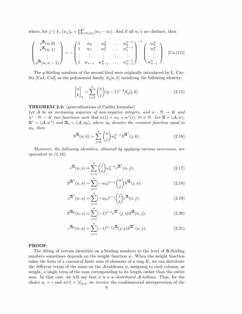
where, for j ≤ k, (wj)k =∏kl=0,l6=j(wj − wl). And if all wi’s are distinct, then

sA(n, 0)

sA(n, 1)...

sA(n, n− 1)

= −

1 w0 w20 . . . wn−1

0

1 w1 w21 . . . wn−1

1...

......

. . ....

1 wn−1 w2n−1 . . . wn−1

n−1

−1

wn0wn1...

wnn−1

. [Co,(11)]

The q-Stirling numbers of the second kind were originally introduced by L. Car-litz [Ca1, Ca2] as the polynomial family Sq[n, k] satisfying the following identity:

[

n

k

]

q

=n

∑

j=k

(

n

j

)

(q − 1)j−kSq [j, k]. (2.15)

THEOREM 2.2: (generalizations of Carlitz formulae)Let A be an increasing sequence of non-negative integers, and w : N → K andw∗ : N → K two functions such that w(i) = w0 + w∗(i), ∀i ∈ N. Let A = (A, w),A∗ = (A, w∗) and A0 = (A,w0), where w0 denotes the constant function equal to

w0, then

SA(n, k) =n

∑

j=k

(

n

j

)

wn−j0 SA

∗

(j, k). (2.16)

Moreover, the following identities, obtained by applying various inversions, areequivalent to (2.16).

cA(n, s) =n

∑

j=s

(

j

s

)

wj−s0 cA

∗

(n, j); (2.17)

SA∗

(n, s) =n

∑

j=s

(−w0)n−j

(

n

j

)

SA(j, s); (2.18)

cA∗

(n, s) =

n∑

j=s

(−w0)j−s

(

j

s

)

cA(n, j); (2.19)

SA0(n, s) =n

∑

j=s

(−1)j−scA∗

(j, s)SA(n, j); (2.20)

cA0(n, s) =n

∑

j=s

(−1)n−jcA(j, s)SA∗

(n, j). (2.21)

PROOF:

The lifting of certain identities on q-Stirling numbers to the level of A-Stirlingnumbers sometimes depends on the weight function w. When the weight functiontakes the form of a canonical finite sum of elements of a ring K, we can distributethe different terms of the sums on the A-tableaux φ, assigning to each column, asweight, a single term of the sum corresponding to its length rather than the entiresum. In that case, we will say that φ is a w-distributed A-tableau. Thus, for thechoice ai = i and w(i) = [i]p,q , we recover the combinatorial interpretation of the

8

p, q-Stirling numbers of both kinds in terms of 0–1 tableaux. Indeed, instead ofattributing a global weight of the form [i]p,q = pi−1 +pi−2q+ . . .+qi−1 to a columnof length i, we associate to each monomial pjqi−j−1 the choice of the (j + 1)-thposition for the 1, giving j non-inversions and (i− j − 1) inversions.

Coming back to Theorem 2.2, since w (in the pair A = (A, w)) is a canonicalsum of two terms, we can talk about w-distributed A-tableaux. For these A-tableaux, each column of length ai will have weight either w0 or w∗(ai). We givehere the general idea of the combinatorial proofs, leaving out the details. See [dMLe](Theorem 4.1 and Proposition 4.2) for similar proofs.

To prove identities (2.16) and (2.17), essentially choose the columns of the w-distributed A-tableaux with weights different from w0.

For (2.18) and (2.19), the right-hand side counts w-distributed A-tableaux withsome columns of weight w0 distinguished, each contributing a factor (−1) to theglobal weight. We can construct a weight-preserving sign-reversing involution onthese tableaux, such that the fixed points are all w-distributed A-tableaux withno column of weight w0, hence giving the left-hand side of the identities. Theinvolution just “changes the status” of the leftmost column of weight w0 in thew-distributed A-tableaux.

For identities (2.20) and (2.21), weight-preserving sign-reversing involutions re-sembling those used to show orthogonality can be designed. �

Theorem 2.2 deals essentially with interactions between A-Stirling numbers wherethe weight functions differ by an additive constant. The next proposition examineswhat happens when the weight functions differ by a multiplicative constant.

PROPOSITION 2.3: Let A = (A, w) where w : N −→ K, and let a ∈ K.Denote by aw the function from N to the ring K obtained by multiplication of w bythe constant a. Then,

c(A,aw)(n, k) = an−kc(A,w)(n, k), (2.22)

S(A,aw)(n, k) = an−kS(A,w)(n, k). (2.23)

PROOF:

It suffices to note that for every A-tableau φ having k columns, the weight of φaccording to weight function aw, (aw)(A,aw)(φ), is related to the weight wA(φ) =

w(A,w)(φ) in the following way:

(aw)(A,aw)(φ) = ak · w(A,w)(φ). �

REMARKS 2.4: Observe that the exact algebraic expressions for cases (7) and(9) of Table 1 can be obtained from cases (6) and (8) (with p = 1) respectively, viaProposition 2.3.

The particular case ai = i, w0 = 1, and w∗(i) = qi − 1 in Theorem 2.2 givesCarlitz’s identity and its close relatives (cf [dMLe], (4.5) to (4.10)), correspondingto cases (6) and (9) of Table 1. The original combinatorial proofs used a unifiedcombinatorial model, q-tableaux, that is fillings of Ferrers diagram with elements ofthe set {0, 1, 2, . . . , q − 1}, q ∈ N.

9

Another application of Theorem 2.2 is the following: M. Koutras [Ko] defined thenon-central Stirling numbers of the first and second kinds c(a)(n, k) and S(a)(n, k)(case (11) of Table 1) to be the polynomials satisfying

t(t− 1) . . . (t− n+ 1) =n

∑

k=0

(−1)n−kc(a)(n, k)(t− a)k (2.24)

and

(t− a)n =n

∑

k=0

S(a)(n, k)t(t− 1) . . . (t− k + 1), (2.25)

Setting x = (t−a) in the previous identities and comparing with (2.3) and (2.5), we

deduce that c(a)(n, k) = cA(n, k) and S(a)(n, k) = SA(n, k), for A = (A, w), whereA = (i)i≥0, and w(i) = −a + i. Formulae (2.16) and (2.17) of Theorem 2.2 thenlet us express the non-central Stirling numbers of Koutras in terms of the usual“central” Stirling numbers (case (2) of Table 1):

c(a)(n, s) =n

∑

j=s

(

j

s

)

(−a)j−sc(n, j), (2.26)

S(a)(n, k) =n

∑

j=k

(

n

j

)

(−a)n−jS(j, k). (2.27)

COROLLARY 2.5:

Let A = (A, w). If the following equality holds for all i ≥ 0

w(ai) = w0 + w0z + w0z2 + . . . + w0z

i−1 = w0[i]z ∈ N[w0, z],

then

cA(n+ 1, k + 1) =n

∑

j=k

(

j

k

)

wj−k0 zn−jcA(n, j), (2.28)

SA(n+ 1, k + 1) =

n∑

m=k

(

n

m

)

wn−m0 zm−kSA(m,k). (2.29)

PROOF: Identity (2.28) (respectively (2.29)) follows from (2.17) and (2.22) (re-spectively (2.16) and (2.23)). The combinatorial proofs are similar to the ones of(2.11) and (2.12) of [dMLe], using w-distributed A-tableaux. �

THEOREM 2.6: (convolution formulae)Let A = (A, w), where A = (a0, a1, a2, . . . ). Denote by δA the sequence (a1, a2, . . . ),and, more generally, by δnA = δ(δn−1A) the sequence (an, an+1, an+2, . . . ). More-over, denote δnA = (δnA, w). Then

cA(m+ j, n) =n

∑

k=0

cA(m,k)cδm

A(j, n− k), (2.30)

SA(m+ j, n) =n

∑

k=0

SA(m,k)SδkA(j, n− k). (2.31)

[VS,(5.18)]10

Likewise,

cA(n+ 1,m+ j + 1) =n

∑

k=0

cA(k,m)cδk+1

A(n− k, j), (2.32)

SA(n+ 1,m+ j + 1) =

n∑

k=0

SA(k,m)Sδm+1

A(n− k, j). (2.33)

[VS,(5.19)]

PROOF:

To prove these formulae combinatorially, one must strategically section the A-tableaux into two parts.

For instance, one gets identity (2.30) (respectively (2.33)) by separating the

columns of theA-tableaux in the set TdA(m+j−1,m+j−n) (respectively TA(m+j + 1, n−m− j)) to form an A-tableau with column lengths in {a0, a1, . . . , am−1}(respectively {a0, a1, . . . , am}), and another A-tableau with column lengths in{am, am+1, . . . , am+j−1} (respectively {am+1, am+2, . . . , am+j+1} for (2.33)).

For identities (2.31) and (2.32), if φ ∈ TA(n,m + j − n) (respectively φ′ ∈

TdA(n, n − m − j)), we must first determine the unique integer k0, 0 ≤ k0 ≤ n

(respectively k1, m ≤ k1 ≤ n), such that

(k0 − 1) + |φ|0 + |φ|1 + . . . + |φ|k0−1 < m

≤ k0 + |φ|0 + |φ|1 + . . . + |φ|k0(2.34)

(respectively

k1 − |φ′|0 − |φ′|1 − . . . − |φ′|k1−1 = m

< (k1 + 1)− |φ′|0 − |φ′|1 − . . . − |φ′|k1), (2.35)

where |φ|i denotes the number of columns of length ai in φ. Note that since φ′

has columns of distinct lengths, (2.35) can only be satisfed if |φ′|k1= 0. The

A-tableau φ (respectively φ′) is then divided into an A-tableau containing the(m − k0) last columns of φ (respectively (k1 − m) last columns of φ′), with col-umn lengths in the set {a0, a1, . . . , ak0

} (respectively {a0, a1, . . . , ak1−1}), and theremaining A-tableau, with column lengths in the set {ak0

, ak0+1, . . . , an} (respec-tively {ak1+1, ak1+2, . . . , an}). �

These identities are generalizations of the convolution formulae (1.11) to (1.14)stated in the introduction, where ai = i and w(i) = [i]q .

As observed in Proposition 2.1, the A-Stirling numbers can be expressed in terms

of the elementary and complete symmetric functions respectively, as cA(n, k) =en−k(w0, w1, . . . ,

wn−1) and SA(n, k) = hn−k(w0, w1, . . . , wk) respectively. Some interesting in-stances of these families of numbers are given by Whitney numbers of supersolvablelattices (cf Stanley [St1, St2]). Other combinatorial properties of generalized Stir-ling numbers will be inherited from properties of symmetric functions. An exampleis logarithmic concavity (see Comtet [Co], Habsieger [Ha], Leroux [Le], and Sagan[Sa]), an aspect which is not treated in the present paper.

11

3. PARTIAL STIRLING NUMBERS AND WEAK 0–1 TABLEAUX

DEFINITIONS 3.1: A weak 0–1 tableau ψ is a triple ψ = (λ, l, f), whereλ = (λ1 ≥ λ2 ≥ . . . ≥ λk) is a partition of an integer m, l is an integer greateror equal to λ1, and f = (fij)1≤j≤λi is a filling of the cells of the correspondingFerrers diagram of shape λ with 0’s and 1’s, such that there is at most one 1 in eachcolumn. We will say that ψ contains l columns, (l − λ1) of which being of lengthzero and considered filled with 0’s.

For example, the weak 0–1 tableau ψ = (λ, l, f) where λ = (5, 4, 2, 2), l = 6 andf13 = f24 = f32 = 1, fij = 0 elsewhere (1 ≤ j ≤ λi) is illustrated in Figure 2.

0 0 1 0 0

0 0 0 1

0 1

0 0

FIGURE 2: weak 0–1 tableau ψ

As for the usual 0–1 tableaux, the inversion number of a weak 0–1 tableau ψ,denoted by inv(ψ), is equal to the number of 0’s below a 1 in ψ. However, thenon-inversions number of ψ, denoted by nin(ψ), is equal to the number of 0’s abovea 1 in ψ, plus the number of 0’s in the columns filled with 0’s. For instance, for ψin Figure 2, we compute inv(ψ) = 2 and nin(ψ) = 8.

We will denote by Tw(h, r) (respectively Tw(h, s, r)), the set of all weak 0–1tableaux ψ = (λ, r, f) containing r columns of length less or equal to h (and havingexactly (r − s) 1’s in the filling f respectively), and by Tdw(h, r) (respectivelyTdw(h, s, r)), the subset of Tw(h, r) (respectively Tw(h, r, s)) consisting of all weak0–1 tableaux with distinct column lengths.

DEFINITIONS 3.2: The partial p, q-Stirling numbers are given by:

Pcp,q[n,m, k] :=∑

ψ∈Tdw(n−1,n−m,n−k)

pnin(ψ)qinv(ψ); (3.1)

PSp,q[n,m, k] :=∑

ψ∈Tw(k,n−m,n−k)

pnin(ψ)qinv(ψ); (3.2)

Pcp,q[n, k] :=∑

ψ∈Tdw(n−1,n−k)

pnin(ψ)qinv(ψ); (3.3)

PSp,q[n, k] :=∑

ψ∈Tw(k,n−k)

pnin(ψ)qinv(ψ). (3.4)

Note that these polynomials are not symmetric in p and q, and that

Pcp,q[n, k] =n

∑

m=k

Pcp,q[n,m, k], (3.5)

PSp,q[n, k] =n

∑

m=k

PSp,q[n,m, k]. (3.6)

12

Like classical Stirling numbers, the partial Stirling numbers have a combinatorialinterpretation in terms of permutations and set partitions, or more precisely, interms of permutations with marked cycles and partial set partitions. To show this,we shall exhibit bijections between weak 0–1 tableaux and these objects. Thecorresponding statistics, obtained by carrying the inversion number and the non-inversion number along the bijections will then provide an alternate interpretationfor the partial p, q-Stirling numbers. We need some definitions and notations.

DEFINITIONS 3.3: Let σ ∈ S(n, l, k) be a permutation of {1, 2, . . . , n} = [[n]],with k cycles such that l of them are marked. We will say that σ is writtenas standard product of cycles if σ is written as a product of disjoint cycles, eachcycle starting with its minimum, and the cycles are ordered by increasing minima.We will denote by w(σ) the word obtained by supressing the parenthesis in thepermutation σ written as a standard product of cycles. The minimum of each cycleis called the cycle leader. To indicate a marked cycle, we will underline its cycleleader. For instance, σ = (1, 9, 3, 5)(2, 7)(4)(6, 10, 8) ∈ S(10, 2, 4) is written as astandard product of cycles, both cycles (2, 7) and (4) are marked, the cycle leadersare respectively 1, 2, 4 and 6, and w(σ) = 1 9 3 5 2 7 4 6 10 8.

There is a natural bijection Φ1 between the sets Tdw(n − 1, l, n − k + l) andS(n, l, k), that is inspired from the recurrence relations (3.20) or (3.26). Let ψ ∈Tdw(n−1, l, n−k+ l). We construct by induction a sequence of permutations withmarked cycles σ0, σ1, . . . , σn such that σi has support [[i]]. The image of ψ under Φ1

will then be Φ1(ψ) = σn. We start with σ0 = ∅, the empty permutation. Supposewe have already determined σ0, σ1, . . . , σi−1, 1 ≤ i ≤ n. Then σi is obtained fromσi−1 in the following way:i) if ψ does not contain a column of length (i − 1), σi coincides with σi−1 on the

set [[i− 1]], and i forms a new unmarked cycle of length one in σi;ii) if ψ contains a column of length (i− 1) filled with 0’s, σi coincides with σi−1 on

the set [[i − 1]], and i forms a new marked cycle of length one in σi;iii) if ψ contains a column of length (i − 1) with a 1 in the j-th cell (from top to

bottom), 1 ≤ j ≤ (i − 1), then σi is obtained from σi−1 by inserting i as theimage of the j-th letter in w(σi−1). The image of i is then set equal to the imageof that letter in σi−1.For example, for ψ ∈ Tdw(5, 2, 5) given in Figure 3, σ0 = ∅, σ1 = (1), σ2 =

(1, 2), σ3 = (1, 2)(3), σ4 = (1, 2)(3)(4), σ5 = (1, 2)(3, 5)(4), and Φ1(ψ) = σ6 =(1, 2)(3, 5, 6)(4). It is easy to see that Φ1 is a bijection. Details are left to thereader.

0 0 0 1

0 0 0

0 1

1 0

0

FIGURE 3: weak 0-1 tableauψ ∈ Tdf(5, 5, 2)

The bijection Φ1 lets us define inversion and non-inversion statistics on permu-tations with marked cycles:

inv(σ) = inv(Φ−11 (σ)), and nin(σ) = nin(Φ−1

1 (σ)). (3.7)13

In fact, it is not hard to see that the inversion number of σ ∈ S(n, l, k) is equalto

inv(σ) = inv(w(σ)), (3.8)

where inv(w(σ)) is the number of inversions in the word w(σ), that is the numberof pairs of letters (i, j) such that j lies to the right of i in w(σ), but j < i, and thenon-inversion number is equal to

nin(σ) =∑

i

(i− 2− invσ(i)) +∑

j

(j − 1), (3.9)

where the first sum ranges over all integer i ∈ [[n]] not cycle leaders, invσ(i) is justthe number of inversions (i, j) in w(σ) with i as first coordinate, and the secondsum ranges over the marked cycles leaders.

DEFINITIONS 3.4: A partial partition (E;π) ∈ PP(n, l, k) of [[n]] is a pair(E;π) such that E is a subset of [[n]] = {1, 2, . . . , n} of cardinality l, and π =π1, π2, . . . , πk is a partition with exactly k blocks of the set [[n]] − E. We will saythat (E;π) is written in standard form if the elements of E appear in increasingorder, each block of π is written by increasing order of its elements, and the blocksare ordered by increasing minima. The blocks minima, a1, a2, . . . , ak respectively,are called block leaders. For example, (E;π) ∈ PP(10, 2, 3), with E = {5, 9} andπ = π1, π2, π3 = {1, 3, 7}, {2, 6, 10}, {4, 8}, is written in standard form and the blockleaders of π are equal to a1 = 1, a2 = 2 and a3 = 4.

We now construct a bijection Φ2 between the sets Tw(k, l, n−k+l) andPP(n, l, k),inspired from the recurrence relations (3.21) or (3.27). Let ψ ∈ Tw(k, l, n− k + l).Transport ψ in the third quadrant by a vertical reflection (so that the columnsare now by increasing order of length). For 1 ≤ i ≤ k, add a column of lengthi, with a 1 in the bottom cell, to the left of the columns of length greater orequal to i (in ψ reflected). Then add cells filled with 0’s to the bottom of eachcolumn so that they reach length k. We obtain a k × n matrix with at mostone 1 in each column (these manipulation are shown in Figure 4 for the weak0–1 tableau of Figure 2). It is the row-to-column representation of the restricted-growth function associated with the partial partition Φ2(ψ) = (E;π) (cf Milne[Mi]). More precisely, if the j-th column of the matrix contains only 0’s, thenj ∈ E, and if the j-th column contains a 1 in the m-th row, then j lies inthe m-th block of the partition π, written in standard form. For example, forψ ∈ Tw(5, 3, 6) illustrated in Figure 2, we obtain the matrix of Figure 4, andΦ2(ψ) = (E;π) = ({1, 3, 10}; {2, 6}, {4, 5}, {7, 9}, {8}, {11}) ∈ PP(11, 3, 5). Φ2 isclearly a bijection.

Once again, carrying over Φ2 the inversion and non-inversion statistics, we obtainthe inversion number of a partial partition (E;π),

inv(E;π) =∑

i∈[[n]]−E

invπ(i), (3.10)

where, if a1 < a2 < . . . < ak are the block leaders of π and i lies in the m-th blockπj , invπ(i) is equal to the number of aj , m < j ≤ k, such that aj < i.

14

0000010001

00000011

00101

0001

1

m

0 1 0 0 0 1 0 0 0 0 00 0 0 1 1 0 0 0 0 0 00 0 0 0 0 0 1 0 1 0 00 0 0 0 0 0 0 1 0 0 00 0 0 0 0 0 0 0 0 0 1

FIGURE 4: construction of a matrix froma weak 0–1 tableau

Moreover, if we let

ninπ(i) =

|{aj | aj < i}| if i ∈ E,

|{aj | 1 ≤ j < m and aj < i}| if i lies in the m-th block of π

(= m− 1) and i is not a block leader,

0 if i is a block leader,(3.11)

then the non-inversion number of a partial partition (E;π) equals

nin(E;π) =∑

i∈[[n]]

ninπ(i),

=

k−1∑

i=0

i (|πi+1| − 1) +∑

j∈E

ninπ(j). (3.12)

¿From these two bijections Φ1 and Φ2, we can deduce

PROPOSITION 3.5: (alternative combinatorial models)With the preceding notations and definitions,

Pcp,q[n,m, k] =∑

σ∈S(n,n−m,n−m+k)

pnin(σ)qinv(σ), (3.13)

PSp,q[n,m, k] =∑

(E;π)∈PP(n,n−m,k)

pnin(E;π)qinv(E;π). (3.14)

Using these alternate interpretations, the generating series for the p = q = 1case are easy to find: PROPOSITION 3.6: (generating series)

15

We have

∑

n,m,k≥0

Pc1,1[n, n−m,k]amukxn

n!= (1− x)−(a+u), (3.15)

∑

n,m,k≥0

PS1,1[n, n−m,k]amukxn

n!= eaxeu(ex−1), (3.16)

∑

n,k≥0

Pc1,1[n, k]uk x

n

n!= (1− x)−(1+u), (3.17)

∑

n,k≥0

PS1,1[n, k]uk x

n

n!= exeu(ex−1). (3.18)

PROOF:

The generating series of permutations according to the number of cycles (weightedby u) is well-known, it is

∑

n≥0

∑

k≥0

c(n, k)ukxn

n!=

(

1

1− x

)u

. (3.19)

Identity (3.15) can be deduced from the fact that a permutation with markedcycles decomposes naturally into two permutations, one containing the markedcycles (weighted by a), and the other the unmarked cycles (weighted by u).

Identity (3.16) expresses the fact that a partial partition (E;π) consists of a setE (each element weighted by a) and a partition π, which is a set of non-emptyblocks (with each block weighted by u).

Identities (3.17) and (3.18) follow from (3.15) and (3.16) and the connections(3.5) and (3.6) between the partial p, q-Stirling numbers with three parameters andthe partial p, q-Stirling numbers with two parameters. �

REMARK 3.7: The basic recurrence relations for the partial p, q-Stirling numberswith two parameters are given by

Pcp,q[n+ 1, k] = Pcp,q[n, k − 1] + (pn + [n]p,q)Pcp,q[n, k], (3.20)

PSp,q[n+ 1, k] = PSp,q[n, k − 1] + (pk + [k]p,q)PSp,q[n, k], (3.21)

with initial boundary conditions Pcp,q[n, k] = 0 = PSp,q[n, k] if k > n, Pcp,q[n, 0] =(p+[1]p,q)(p

2 +[2]p,q) . . . (pn−1 +[n−1]p,q), PSp,q[n, 0] = 1 and Pcp,q[0, k] = δ0,k =

PSp,q[0, k].Separating the different possibilities for the leftmost column of weak 0–1 tableaux

(length not equal to the maximal allowed value, or length equal to the maximalvalue with the filling containing a 1 or no 1) gives a combinatorial proof of theserecurrence relations.

Comparing (3.20) and (3.21) to (1.9) and (1.10) yields the conclusion that thesefamilies of polynomials are special cases of A-Stirling numbers (for A = (A, w),where A = (i)i≥0 and w(i) = pi + [i]p,q), and thus every identity in the previoussection applies to them. However, it is not the case for the sequences (Pcp,q[n,m, k])and (PSp,q[n,m, k]), for which a more detailed analysis is necessary.

16

PROPOSITION 3.8: The following identities hold for the partial p, q-Stirlingnumbers with three parameters Pcp,q[n,m, k] and PSp,q[n,m, k]:a) (connections and special cases)

Pcp,q[n, n, k] = cp,q[n, k] and Pcp,q[n, k, k] = p(n−k

2 )[

n

k

]

p

, (3.22)

PSp,q[n, n, k] = Sp,q[n, k] and PSp,q[n, k, k] =

[

n

k

]

p

, (3.23)

Pc1,q[n,m, k] =

(

n−m+ k

k

)

cq[n, n−m+ k], (3.24)

PS1,q [n,m, k] =

(

n

m

)

Sq[m,k]; (3.25)

b) (recurrence relations)

Pcp,q[n+ 1,m+ 1, k] =Pcp,q[n,m, k − 1] + pnPcp,q[n,m+ 1, k]+

[n]p,qPcp,q[n,m, k], (3.26)

PSp,q[n+ 1,m+ 1, k] =PSp,q[n,m, k − 1] + pkPSp,q[n,m+ 1, k]

+ [k]p,qPSp,q[n,m, k], (3.27)

with initial boundary conditionsPcp,q[n,m, k] = 0 = PSp,q[n,m, k] if m > n or if k > m,Pcp,q[0,m, k] = δ0,kδ0,m, PSp,q[0,m, k] = δ0,kδ0,m,

Pcp,q[n, 0, k] = p(n

2)δk,0, PSp,q[n, 0, k] = δ0,k,

and Pcp,q[n,m, 0] = p(n

2)−mc1,q/p[n, n−m], PSp,q[n,m, 0] = δm,0;c) (generating series)

For n > 0,

∑

r≥0

∑

m≥0

Pcp,q[n,m, r]xrym−rzn−m (3.28)

=(x+ z)(x+ pz + [1]p,qy) . . . (x+ pn−1z + [n− 1]p,qy),

for k ≥ 0,

∑

r≥0

∑

l≥0

PSp,q[k + r, k + l, k]xlyr−l = (3.29)

1

(1− y)

1

(1− py − [1]p,qx)

1

(1− p2y − [2]p,qx). . .

1

(1− pky − [k]p,qx).

PROOF:

a) When n = m, this forces all the columns of the weak 0–1 tableaux to containa 1 so Pcp,q[n, n, k] and PSp,q[n, n, k] are counting usual 0–1 tableaux according toinversion and non-inversion numbers.

17

When m = k, the corresponding weak 0–1 tableaux must be filled with 0’s only,each 0 contributing to a factor p, thus yielding the combinatorial interpretation ofthe q-binomial coefficients in terms of partitions fitting in a box.

Identities (3.24) and (3.25) become obvious with the alternate combinatorialinterpretations of Proposition 3.5. Indeed, Pc1,q[n,m, k] is q-counting (accordingto inversion number) permutations of [[n]] with (n−m+ k) cycles (factor cq[n, n−m + k] on the right-hand side of (3.24)), such that (n − m) of these cycles are

marked (there is(

n−m+kn−m

)

ways of choosing them among the (n − m + k) cycles

of the permutations). Likewise, PS1,q [n,m, k] is q-counting (according to inversionnumber) partial partitions (E;π) of the set [[n]] such that |E| = (n−m) (the factor(

nm

)

on the right-hand side of (3.25) corresponds to the choice of E) and π is apartition with exactly k blocks (corresponding to the factor Sq [m,k]).

b) The proofs of (3.28) and (3.29) are similar to those of (3.20) and (3.21). Notethat the weak 0–1 tableaux ψ ∈ Tdw(n− 1, n−m,n) all have a “staircase” shape(the lengths of the columns are respectively (n − 1), (n − 2), . . . , 1 and 0). Tocompute their non-inversion number, we need only substract the inversion numberand the number m of 1’s in the filling to the total number of cells of ψ. This gives

the initial boundary condition Pcp,q[n,m, 0] = p(n

2)−mc1,q/p[n, n−m].c) (3.28) and (3.29) easily follow from the combinatorial definition. �

In addition to identities (3.24) and (3.25), partial Stirling numbers can also beexpressed in terms of usual q-Stirling numbers in the following way (for p = 1):

PROPOSITION 3.9: We have:

Pc1,q[n+ 1, k + 1] =

n∑

j=k

[(

j + 1

k + 1

)

+

(

j

k

)]

2j−k−1qn−jcq[n, j], (3.30)

PS1,q [n+ 1, k + 1] =n

∑

j=0

[

n−j∑

i=0

(

n− i

j

)

2n−j−i

]

qj−kSq[j, k], (3.31)

Pc1,q[n+ 1,m+ 1, k + 1] (3.32)

=n

∑

j=k

[(

j

k

)(

j − k

n−m

)

+

(

j

k + 1

)(

j − k − 1

n−m− 1

)]

qn−jcq[n, j],

PS1,q[n+ 1,m+ 1, k + 1]

=n

∑

j=0

[

n−j∑

i=0

(

n− i

j

)(

n− j − i

n−m− i

)

]

qj−kSq [j, k]. (3.33)

PROOF:

These identities are proven similarly to (2.11) and (2.12) in [dMLe]. We essen-tially remove the columns causing no inversions. Thus all the remaining columnsmust contain a 0 in the bottom cell and a 1 somewhere above it. By deleting thesebottom cells, we obtain a general 0–1 tableau. The difference with the identities(2.11) and (2.12) of [dMLe] is that there are two kinds of columns that do not

18

cause any inversion: the columns filled exclusively with 0’s and the columns whichcontain a 1 positionned in the bottom cell. Details are left to the reader. �

PROPOSITION 3.10: (convolution formulae)We have:

cp,q[m+ n, k] =∑

i+j≥k

pn(i+j−k) [n]m−jp,q cp,q[n, i] Pcq,p[m, j, k − i], (3.34)

Sp,q[m+ n, k] =∑

i+j≥k

pi(i+j−k) [i]m−jp,q Sp,q[n, i] PSq,p[m, j, k − i]. (3.35)

cp,q[n+ 1,m+ j + 1] =

n∑

k=0

n−k∑

i=j

p(k+1)(i−j) [k + 1]n−k−ip,q cp,q[k,m] Pcq,p[n− k, i, j],

(3.36)

Sp,q[n+1,m+ j+1] =n

∑

k=0

n−k∑

i=j

p(m+1)(i−j) [m+1]n−k−ip,q Sp,q[k,m] PSq,p[n−k, i, j].

(3.37)

PROOF:

These identities are particular cases of Theorem 2.6, with A = (i)i≥0 and w(i) =

[i]p,q . For these parameters, cA(n, k) = cp,q[n, k], SA(n, k) = Sp,q[n, k],

cδm

A(n, k) =∑

ϕ∈Td≥m(n−1,n−k)

pnin(ϕ) qinv(ϕ),

andSδ

mA(n, k) =

∑

ϕ∈T≥m(k,n−k)

pnin(ϕ) qinv(ϕ),

where T≥m(h, r) (respectively Td≥m(h, r)) denotes the subset of T (h + m, r) (re-spectively Td(h + m, r)) containing all the 0–1 tableaux ϕ such that the lengthof each column is at least equal to m. The notations T (h, r) and Td(h, r) wereintroduced in Section 1.

The 0–1 tableaux ϕ ∈ Td≥m(n− 1, n− k) (respectively ϕ ∈ T≥m(k, n− k)) canbe decomposed into a rectangular weak 0–1 tableau ψ1 of format m× (n− k), anda general weak 0–1 tableau ψ2 ∈ Td(n−1, n−k) (or ψ2 ∈ T (k, n−k) respectively),such that the columns of ψ1 containing a 1 correspond exactly to the columns of ψ2

filled with 0’s, and vice-versa. The enumeration of these pairs of weak 0–1 tableauxaccording to inversion and non-inversion numbers leads to

cδm

A(n, k) =n

∑

i=k

pm(i−k) [m]n−ip,q Pcq,p[n, i, k], (3.38)

Sδm

A(n, k) =n

∑

i=k

pm(i−k) [m]n−ip,q PSq,p[n, i, k]. (3.39)

Details are left to the reader. �

19

Note that (3.34) to (3.37) are p, q-analogues of identities (1.11) to (1.14), thusproviding a complete answer to the first question that was adressed to us.

4. IDENTITIES RELATED TO 0–1 TABLEAUX WHOSE COLUMN

LENGTHS ARE RESTRICTED TO AN ARITHMETIC PROGRES-

SION

In this section, we study A-tableaux for which w(ai) = [a+ id]p,q, a, d ∈ N, thep, q-analogue of an arithmetic progression. This particular case can be realized intwo different ways.

The first possibility Aap = (a+ id)i≥0 and wap : N → N[p, q] such that wap(k) =[k]p,q, corresponds combinatorially to the p, q-counting of 0–1 tableaux whose col-umn lengths are part of the arithmetic progression {a+ id}i≥0. More precisely, fixa and d ∈ N. We will denote by T a,d(h, r) (respectively Tda,d(h, r)) the subset ofT (a + hd, r) (respectively Td(a + hd, r)) containing all 0–1 tableaux with columnlengths belonging to the set {a, a + d, a + 2d, . . . , a + hd}. The notations T (h, r)and Td(h, r) were introduced in Section 1. Note that if a = 0, since [0]p,q = 0,the column lengths will be elements of the set {d, 2d, . . . , hd}. If d = 0, the 0–1tableaux are degenerate and contain only columns of length a. However, this casecan be included if we distinguish between the different lengths (a + i · 0), i ≥ 0.A way to do this is to associate to the 0–1 tableaux ϕ of format a ×m partitionsµ = µ1 ≥ µ2 ≥ . . . ≥ µm ≥ 0, corresponding to these different i’s.

We then have

c(Aap,wap)(n, k) =∑

ϕ∈Tda,d(n−1,n−k)

pnin(ϕ)qinv(ϕ), (4.1)

and

S(Aap,wap)(n, k) =∑

ϕ∈Ta,d(k,n−k)

pnin(ϕ)qinv(ϕ). (4.2)

The second possibility is Acw = (Acw, wcw), where Acw = (i)i≥0 and

wcw(k) = [a+ kd]p,q = pkd[a]p,q + qa[d]p,q[k]pd,qd . (4.3)

This decomposition of the weight function suggests a combinatorial interpreta-tion in terms of p, q-counting of coloured weak 0–1 tableaux.

DEFINITION 4.1: A coloured weak 0–1 tableau consists of a pair (ψ, γ) suchthat ψ = (λ, l, f) is a weak 0–1 tableau, and γ : Cψ → {0, 1, 2, . . . , a + d − 1}is a “colouring” of the columns c of ψ with colors γ(c), satisfying the followingconditions:i) if the column c is filled with 0’s, then 0 ≤ γ(c) ≤ (a− 1), andii) if the filling of c contains a 1, then a ≤ γ(c) ≤ (a+ d− 1).

By convention, if a = 0, the weak 0–1 tableau ψ contains no columns filled with0’s, and if d = 0, ψ contains no columns with 1’s.

We will denote by Tcw(h, r) (respectively Tdcw(h, r)) the set of all colouredweak 0–1 tableaux (ψ, γ) such that ψ ∈ Tw(h, r) (respectively ψ ∈ Tdw(h, r)). Thenotations Tw(h, r) and Tdw(h, r) were introduced in Section 3.

20

DEFINITION 4.2: Let (ψ, γ) be a coloured weak 0–1 tableau. The p, q-weightwp,q(γ) of the colouring γ is given by the following expression:

wp,q(γ) =∏

c∈Cψ

wp(c)wq(c), (4.4)

where Cψ denotes the set of columns (of length possibly null) of the weak 0–1tableau ψ = (λ, l, f),

wp(c) =

{

pa−1−γ(c) if c is filled with 0’s,

pa+d−1−γ(c) if c contains a 1;(4.5)

andwq(c) = qγ(c). (4.6)

For example, if a = 2, d = 3, and ψ is the weak 0–1 tableau illustrated in Figure2, a possible colouring γ of ψ would be γ(c1) = 0, γ(c2) = 4, γ(c3) = 4, γ(c4) = 2,γ(c5) = 1, and γ(c6) = 1, where c1, c2, . . . , c6 denote the columns of ψ from left toright, and the p, q-weight of γ is equal to wp,q(ψ, γ) = p1+0+0+2+0+0q0+4+4+2+1+1 =p3q12.

PROPOSITION 4.3: With the preceding notations,

c(Acw,wcw)(n, k) =∑

(ψ,γ)∈Tdcw(n−1,n−k)

pd×nin(ψ)qd×inv(ψ)wp,q(γ), (4.7)

andS(Acw,wcw)(n, k) =

∑

(ψ,γ)∈Tcw(k,n−k)

pd×nin(ψ)qd×inv(ψ)wp,q(γ). (4.8)

PROOF: We need only see that in

wcw(k) = [a+ kd]p,q = pkd[a]p,q + qa[d]p,q[k]pd,qd ,

the factors pkd and [k]pd,qd correspond to d times the inversion and non-inversionnumbers of weak 0–1 tableaux, and [a]p,q and qa[d]p,q to the p, q-weight of colour-ings. �

There is a natural bijection preserving p, q-counting between coloured weak 0–1tableaux and 0–1 tableaux whose column lengths lie in an arithmetic progression.Let (ψ, γ) = ((λ, l, f), γ) ∈ Tcw(h, r) (respectively Tdcw(h, r)). We map (ψ, γ) into

a 0–1 tableau ϕ = (λ, f) ∈ T a,d(h, r) (respectively Tda,d(h, r)) in the following way:each column cj in ψ of length i is replaced by a column of length (a+ id).i) if the column cj was filled with 0’s and coloured with color γ(cj) = m, 0 ≤ m ≤

(a − 1), we put a 1 in position (id + a −m) (from top to bottom) of the new

column (i.e. fid+a−m,j = 1), andii) if cj had a 1 in position h, 1 ≤ h ≤ i, and was coloured with color γ(cj) = m,

a ≤ m ≤ (a+ d− 1), we put a 1 in position (hd+ a−m) (i.e. fhd+a−m,j = 1).For example, if a = 2, d = 3, h = 5 and r = 6, Figure 5 illustrates the

correspondence. The first row (shaded in the figure) of the tableau on the leftgives the different colors of the columns of the coloured tableau (which is the

21

0 4 4 2 1 1

0 0 1 0 0

0 0 0 1

0 1

0 0

⇐⇒

0 0 1 0 0 1

0 0 0 0 0 0

0 0 0 0 0

0 0 0 0 1

0 0 0 0 0

0 0 0 1

0 1 0 0

0 0 0 0

0 0

0 0

0 0

0 0

0 0

1 0

FIGURE 5: Correspondence between the setsTcw(h, r) and T a,d(h, r)

weak 0–1 tableau of Figure 2). Note that in this example, we have, as expected,wp,q(γ)p

d×nin(ψ)qd×inv(ψ) = p3q12p3×8q3×2 = p27q18 = pnin(ϕ)qinv(ϕ). Details areleft to the reader.

Let ca,dp,q [n, k] and Sa,dp,q [n, k] denote

ca,dp,q [n, k] = c(Aap,wap)(n, k)

= c(Acw,wcw)(n, k), (4.9)

and

Sa,dp,q [n, k] = S(Aap,wap)(n, k)

= S(Acw,wcw)(n, k). (4.10)

We will call these polynomials a, d-progressive p, q-Stirling numbers of first andsecond kinds. As for the partial p, q-Stirling numbers, we can use the correspon-dence between weak 0–1 tableaux and permutations with marked cycles or partialset partitions described in Section 3 to obtain an alternate combinatorial interpre-tations in terms of these objects, enriched with some colouring.

In the remainder of this section, we present various identities on a, d-progressivep, q-Stirling numbers. We will use either combinatorial interpretations in terms of0–1 tableaux to prove these identities, according to the context.

PROPOSITION 4.4:

a) (special cases)

c0,dp,q [n, k] = [d]n−kp,q cpd,qd [n, k], (4.11)

S0,dp,q [n, k] = [d]n−kp,q Spd,qd [n, k]. (4.12)

22

In particular,

c0,1p,q[n, k] = cp,q[n, k] and S0,1p,q [n, k] = Sp,q[n, k]. (4.13)

ca,0p,q [n, k] = [a]n−kp,q

(

n

k

)

, (4.14)

Sa,0p,q [n, k] = [a]n−kp,q

(

n

k

)

. (4.15)

In particular,

c1,0p,q[n, k] =

(

n

k

)

= S1,0p,q [n, k]. (4.16)

c1,1p,q =n

∑

m=k

qm−kPcp,q[n,m, k], (4.17)

S1,1p,q =

n∑

m=k

qm−kPSp,q[n,m, k]. (4.18)

b) (q-analogues of identities of Voigt [Vo])

ca,d1,q [n, j] =

n∑

k=j

(

k

j

)

[a]k−jq qa(n−k)c0,d1,q [n, k], (4.19)

Sa,d1,q [n, j] =

n−j∑

k=0

(

n

k

)

[a]kq qa(n−k−j)S

0,d1,q [n− k, j]. (4.20)

c) (connections with q-Stirling numbers)

ca,d1,q [n, j] =

n∑

k=j

(

k

j

)

[a]k−jq (qa[d]q)n−kcqd [n, k], (4.21)

and

Sa,d1,q [n, j] =

n−j∑

k=0

(

n

k

)

[a]kq (qa[d]q)

n−k−jSqd [n− k, j]. (4.22)

PROOF:

a) For a = 0 and d = 1, both combinatorial models reduce to the usual p, q-counting (according to inversion and non-inversion numbers) of 0–1 tableaux inTd(n− 1, n− k) for c0,1p,q[n, k] and in T (k, n− k) for S0,1

p,q [n, k].Identities (4.11) to (4.16) have simple proofs using either interpretations in terms

of 0–1 tableaux. We will use the coloured weak 0–1 tableau model.The choice a = 0 suppresses all weak 0–1 tableaux containing columns filled

with 0’s (since there are no “colors” to colour them with). Thus only usual 0–1tableaux remain, for which each column is assigned a color between 0 and (d− 1).

23

For a fixed 0–1 tableau ϕ, the p, q-weight of all possible colourings is [d]nc(ϕ)p,q , where

nc(ϕ) denotes the number of columns in ϕ. Moreover, since every inversion andnon-inversion is counted d times, we obtain (4.11) and (4.12).

Choosing d = 0 forces the corresponding weak 0–1 tableaux to be filled with 0’sonly, each column being coloured with some color i between 0 and (a − 1). Notethat since d = 0, inversion and non-iversion numbers of the weak 0–1 tableauxare not taken in account, and we are counting partitions (with (n− k) columns oflength possibly zero) that fit in a box, with some color associated to each column.Possible colourings correspond to the factor [a]n−kp,q on the right-hand side of (4.14)

and (4.15), and partitions (with distinct column lengths or not) to the factor(

nk

)

.In the case a = 1 and d = 1, every column has a single choice of color, that is

color 0 if it is filled with 0’s, or color 1 if it contains a 1. Let (ψ, γ) be a colouredweak 0–1 tableau with such a colouring. Then it is easy to see that wp,q(γ) = qj ,where j is equal to the number of columns in ψ containing a 1. Identities (4.17) and(4.18) follow from the combinatorial interpretation of partial p, q-Stirling numbers(with three parameters) in terms of weak 0–1 tableaux.

b) We want to isolate the contribution of parameter a in ca,d1,q [n, j] and S

a,d1,q [n, j].

Using the interpretation in terms of coloured weak 0–1 tableaux, this means sepa-rating the columns filled with 0’s from the rest of the tableau, remembering theirlengths and their positions (same reasoning as (2.28) and (2.29) or (3.30) to (3.33)).Next, we isolate the q-weight from their colourings (factor [a]q for each column filledwith 0’s), as well as the contribution qa to the q-weight of the colouring of eachcolumn containing a 1. This yields to (4.19) and (4.20).c) (4.21) is deduced from (4.19) and (4.11), and (4.22) is deduced from (4.20) and(4.12). �

The a, d-progressive Stirling numbers being a special case of A-Stirling numbers,all the results of Section 2 apply to them. In particular, we obtain the followingconvolution formulae from Theorem 2.10:

PROPOSITION 4.5: (convolution formulae)

ca,dp,q [m+ j, n] =n

∑

k=0

ca,dp,q [m,k]ca+md,dp,q [j, n− k], (4.23)

Sa,dp,q [m+ j, n] =n

∑

k=0

Sa,dp,q [m,k]Sa+kd,dp,q [j, n− k], (4.24)

ca,dp,q [n+ 1,m+ j + 1] =n

∑

k=0

ca,dp,q [k,m]ca+(k+1)d,dp,q [n− k, j], (4.25)

Sa,dp,q [n+ 1,m+ j + 1] =n

∑

k=0

Sa,dp,q [k,m]Sa+(m+1)d,dp,q [n− k, j]. (4.26)

Note that (4.24) and (4.26) are p, q-analogues of (6.24) and (6.25) of [VS].

PROPOSITION 4.6: (analogue of Corollary 2.5)

ca,dq,1 [n+ 1, k + 1] =

1∑

i=0

[a]iq,1

n−i∑

j=k

(

j + i

j − k

)

[d]j−kq,1 qd(n−i−j)c

a,dq,1 [n, j + i], (4.27)

24

Sa,dq,1 [n+ 1, k + 1] =

n−k∑

i=0

[a]iq,1

n−i∑

m=k

(

n− i

m

)

[d]n−m−iq,1 qd(m−k)Sa,dq,1 [m,k]. (4.28)

PROOF:

The proof uses the same idea as the one of Corollary 2.5. Using the model interms of 0–1 tableaux whose column lengths are part of an arithmetic progression{a + id}i≥0, simply delete every column of length a and every column of lengtha + jd, j ≥ 1, such that the 1 appears in one of the d first rows (from top tobottom). Details are left to the reader. �

PROPOSITION 4.7: (generating series)a) (J.B. Remmel and M. Wachs [ReWa])

∑

n,k≥0

ca,d1,1 [n, k]uk

xn

n!= (1− dx)

−(a+u)d , (4.29)

∑

n,k≥0

Sa,d1,1 [n, k]uk

xn

n!= eaxe

u

(

edx−1d

)

. (4.30)

b) (generalization of case a = 0, d = 1 due to I. Gessel [Ge, (6.1)])

∑

n≥0

∑

k≥0

ca,d1,q [n, k]u

k xn

[n]qd !=

(qa[d]qx; qd)∞

((qa[d]q + (1− qd)([a]q + u))x; qd)∞

, (4.31)

where (p; q)∞ =∏∞i=0(1− pqi).

PROOF:

a) These generating series are trivial using the alternate combinatorial models interms of coloured permutations with marked cycles and coloured partial set par-titions. Note that when p = q = 1, a and d can be considered as weights insteadof colourings. On one hand, the parameter a accounts for the number of markedcycles in the permutations and the number of elements of E, in the partial setpartitions (E;π). On the other hand, d accounts for the number of elements of thepermutations that are not cycle leaders, and the number of elements in the partialset partitions that are not in E nor a block leader. Details are left to the reader.b) Identity (4.31) is obtained by algebraic manipulations on q-series. Let

F (u, t) =∑

n≥0

∑

k≥0

ca,d1,q [n, k]u

k tn

(qd; qd)n, (4.32)

where (a; q)n = (1− a)(1− aq) . . . (1− aqn−1). On one hand,

G(u, t) =∑

n≥0

∑

k≥0

ca,d1,q [n, k]u

k tn−1

(qd; qd)n−1(4.33)

=1

t

(

F (u, t)− F (u, qdt))

. (4.34)

25

And on the other hand, by replacing ca,d1,q [n, k] in (4.33) by the right-hand side ofthe basic recurrence relation

ca,d1,q [n, k] = c

a,d1,q [n− 1, k − 1] + [a+ (n− 1)d]1,qc

a,d1,q [n− 1, k],

we compute

G(u, t) = [a]qF (u, t) + qa[d]q

(1− qd)

(

F (u, t)− F (u, qdt))

+ uF (u, t). (4.35)

Identities (4.34) and (4.35) lead to the functional equation

F (u, t) =

(

1−qd[d]qt

(1− qd)

)

(

1− [a]qt−qa[d]qt

(1− qd)− ut

)F (u, qdt). (4.36)

Finally, iterating (4.36) and replacing t by (1 − qd)x gives the generating series(4.31). �

References

[Bu]L.M. Butler, The q-log concavity of q-binomial coefficients, J. Comb. Th., Series A 54 (1990),

53–62.[Ca1]L. Carlitz, On abelian fields, Trans. Amer. Math. Soc. 35 (1933), 122–136.[Ca2] , q-Bernoulli numbers and polynomials, Duke Math. J. 15 (1948), 987-1000.

[Ch]W.Y. Chen, Context-free grammars, differential operators and formal power series, Actes duColloque sur les series formelles et la combinatoire algebrique (M. Delest, G. Jacob and P.Leroux, ed.), ISSN-1157-3953, Publ. LaBRI, Bordeaux, 1991, pp. 145–160.

[Co]L. Comtet, Nombres de Stirling generaux et fonctions symetriques, C. R. Acad. Sc. Paris 275

(1972), 747–750.[dMLe]A. de Medicis and P. Leroux, A unified combinatorial approach for q-(and p, q-)Stirling num-

bers, J. Stat. Planning and Inference 34 (1993), 89–105.[Do]T.A. Dowling, A class of geometric lattices based on finite groups, J. Comb. Th., Series B 14

(1973), 61–85.

[Ge]I. Gessel, A q-analogue of the exponential formula, Discrete Math. 40 (1982), 69–80.[Go]H.W. Gould, The q-Stirling Numbers of the First and Second Kinds, Duke Math. J. 28 (1961),

281–289.

[Ha]L. Habsieger, Inegalites entre fonctions symetriques elementaires: applications a des problemesde log concavite, Discrete Math. 115 (1993), 167–174.

[Ko]M. Koutras, Non-central Stirling numbers and some applications, Discrete Math. 42 (1982),

73–89.[Le]P. Leroux, Reduced Matrices and q-Log Concavity Properties of q-Stirling Numbers, J. Comb.

Th., Series A 54 (1990), 64–84.[Mi]S.C. Milne, Restricted Growth Functions and Incidence Relations of the Lattice of Partitions

of an n-Set, Adv. in Math. 26 (1977), 290–305.[ReWa]J.B. Remmel and M. Wachs, p, q-analogues of the Stirling numbers, private communication

(1986).

[Ri] Riordan, Combinatorial Identities, Wiley, 1968.[RuVo]A. Rucinski and B. Voigt, A local limit theorem for generalized Stirling numbers, Rev.

Roumaine de Math. Pures 35 no 2 (1990), 161–172.

[Sa]B.E. Sagan, Log concave sequences of symmetric functions and analogs of the Jacobi-Trudideterminants, AMS Trans. 329 (1992), 795–811.

[St1]R.P. Stanley, Supersolvable lattices, Alg. Univ. 2 (1972), 197–217.

[St2] , Finite lattices and Jordan-Holder sets, Alg. Univ. 4 (1974), 361–371.

26

[VS]L. Verde-Star, Interpolation and Combinatorial Functions, Studies in Applied Math. 79

(1988), 65–92.[Vo]B. Voigt, A common generalization of binomial coefficients, Stirling numbers and Gaussian

coefficients, Proc. 11th Winter School on Abstract Analysis (Zelezna Ruda, 1983), Rend. Circ.Math. Palermo, vol. Suppl. no 3, 1984, pp. 339-359.

LACIM, Departement de Mathematiques et Informatique, Universite du Quebec a

Montreal, C.P. 8888, Succursale A, Montreal, Qc, CANADA, H3C 3P8.

27