ORIGINAL PAPER - EXPLORATION GEOPHYSICS

Generalized regression and feed-forward back propagation neuralnetworks in modelling porosity from geophysical well logs

Ahmed Amara Konate • Heping Pan •

Nasir Khan • Jie Huai Yang

Received: 27 December 2013 / Accepted: 21 August 2014 / Published online: 11 September 2014

� The Author(s) 2014. This article is published with open access at Springerlink.com

Abstract Geophysical formation evaluation plays a fun-

damental role in hydrocarbon exploration and production

processes. It is a process which describes different reser-

voir parameters using well field data. Porosity is one of the

parameters that determines the amount of oil present in a

rock formation and research in this area is mainly carried

out by engineers and geoscientists in the petroleum

industry. Accurate prediction of porosity is a difficult

problem. This is mostly due to the failure in the under-

standing of spatial porosity parameter distribution. Artifi-

cial neural networks have proved to be a powerful tool for

mapping complicated and non-linear relationships in

petroleum studies. In this study, we analyze and compare

generalized regression neural network (GRNN) and feed-

forward back propagation neural network (FFBP) in

modeling porosity in Zhenjing oilfield data. This study is

calibrated on four wells of Zhenjing oilfield data. One well

was used to find an empirical relationship between the well

logs and porosity, while the other three wells were used to

test the model’s predictive ability in the field, respectively.

The findings proved that the GRN network can make more

accurate and credible porosity parameter estimation than

the commonly used FFBP network. Artificial intelligence

can be exploited as a powerful instrument for predicting

reservoir properties in geophysical formation evaluation

and reservoir engineering in petroleum industry.

Keywords Porosity prediction � Generalized regression

neural network Feed-forward back propagation �Computational geophysics � Reservoir evaluation �Reservoir properties � Geophysical well logs

Introduction

A major activity in evaluating reservoir is examining the

impact of reservoir heterogeneities on reservoir behavior.

Heterogeneity in evaluating reservoir is referred to as non-

linear and non-uniform spatial distribution of rock prop-

erties such as porosity, permeability and fluids (oil, gas,

water) saturation (Mohaghegh et al. 1996). However, it is

difficult to predict rock properties due to the form and

spatial distribution of these heterogeneities, also the

applicability of traditional analytical techniques such as

multivariate regression are limited in this context. Several

authors such as Mohaghegh et al. (1996) and Handhel

(2009) in their related researches buttress these complexi-

ties for predicting in heterogeneity reservoir in oil and

natural gas field studies.

Understanding the form and spatial distribution of rock

properties is fundamental to a successful characterization

of petroleum reservoirs (Haldorsen and Damsleth 1993;

Wong et al. 1995). In this prevalent situation, it is useful to

construct a model that understands rock properties and has

the capabilities to make a good prediction. To build a

model for predicting requires a set of mathematical equa-

tions which describe the dynamic behavior of the process,

in other words link a number of input variables with a set of

results.

This is a typical problem that can be solved by artificial

neural network (ANN) if the phenomenon to be modeled is

non-linear; such as the one used in this research. ANNs

A. A. Konate � H. Pan (&) � N. Khan � J. H. YangInstitute of Geophysics and Geomatic, China University

of Geosciences, Wuhan 430074, Hubei Province, China

e-mail: panpinge@163.com

A. A. Konate

e-mail: konate77@yahoo.fr

123

J Petrol Explor Prod Technol (2015) 5:157–166

DOI 10.1007/s13202-014-0137-7

(Hecht-Nielsen 1989) offer an alternative that has the

potential to establish a model from non-linear, complex

and multidimensional data. They usually take little time to

predict output response for any input value that falls in the

range of the training data.

Artificial neural network offers real benefit over tradi-

tional modeling, including the ability to handle large

amounts of noisy data from dynamic and nonlinear systems

without a priori information of the processes involved,

ANN provides an adequate solution even when the data are

incomplete or ambiguous (Handhel 2009). One of the

interesting properties of ANN is that it makes accurate

predictions. This predictive ability is that it has a degree of

liberty that allows it to better capture the non-linearity of a

system compared to other modeling techniques.

Artificial neural network has become progressively

popular in the petroleum industry and has been widely

applied in many petroleum industry applications (see

review in van der Baan and Jutten 1992; Poulton 2002). In

most of these publications, the feed-forward back propa-

gation neural network (FFBP) configuration is proposed.

However, despite the popular applications of FFBP as

shown by these publications, the FFBP suffers mostly from

the weight initialization randomly given, and the local

minima problems, which can often lead the model to

evolve in an inaccurate direction. More precisely there are

chances that the model never converges to the optimal

solution. Furthermore, FFBP training time is often slow

and in network architecture optimization, FFBP still have

too much human interferences, i.e. the determination of the

hidden layer and the number of hidden layer neurons still

depend on the user. An alternative way to avoid the above

problem is to employ generalized regression neural net-

work (GRNN). As mentioned by Specht (1991), in GRN

network optimization process only one parameter

(smoothness parameter) has to be adjusted in one pass

through the data; no iterative procedure is required; the

estimate is confined by the minimum and maximum of the

data; convergence guaranteed; fast and stable.

Based on the aforementioned assertions, the researchers

were motivated to propose GRNN to predict porosity using

four geophysical well logs. The prediction performances

were quantified, and compared to FFBP.

Porosity is one of the key petrophysical parameters in

evaluating reservoirs to optimize the production of oil and

natural gas fields. It is one of the factors that determines the

amount of oil present in a rock formation and research in

this area is mostly carried out by engineers and geoscien-

tists in the petroleum industry.

This study focuses on developing a model based on

ANN that is applicable to predict porosity at Zhenjing

oilfield China. It highlights the comparison between GRNN

over FFBP in porosity modeling and estimation on

common testing set. It also as well as examines the model’s

ability to predict porosity in the oilfield.

The findings showed that, GRNN compared to FFBP,

GRNN model for modeling porosity using geophysical

well logs is significant for the geophysical exploration

undertaken in the petroleum industry.

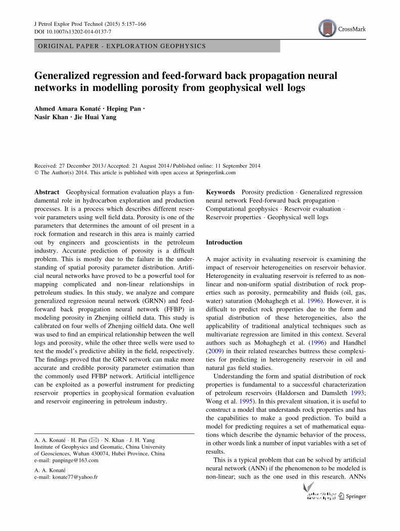
Database

Four wells named Well#A, Well#B, Well#C and Well#D

from Zhenjing oilfield China were used to provide phys-

icals log and core porosity data. The physicals logs con-

sisted of bulk density (DEN), compensated neutron

porosity (CNL), acoustic (AC) and deep induction resis-

tivity (ILD). The DEN, CNL and AC respond to the

characteristics of rock directly adjacent to the borehole. A

combination of these logs provides more accurate esti-

mations of porosity. These geophysical logs are also

known as porosity logs. The difference existing between

these porosity logs is that, the DEN and CNL are nuclear

measurements while AC uses acoustic measurements.

However, ILD is an electric log that measures the resis-

tivity of the un-invaded zone of the formation. A crucial

use of ILD is the determination of hydrocarbon contained

within the pore space of the formations traversed by the

well. Figure 1 shows the geophysical well logs used in

this study.

Logging tool responses are badly affected by breakout

of wall-rock during drilling, as well as stick-and-pull as

logging tools are winched up the well (Yan 2002). Keeping

this in mind, during this study, the data set from the three

wells were carefully examined. All geophysical well logs

which exhibited strange, and possibly inappropriate data

were ignored. In addition, correction of the offset between

core depth and logging depth was done, so that the geo-

physical well logs and experimental data may be matched

and integrated effectively.

The data from Well#A (1046 core and log data) were

chosen to provide the training patterns. This well was

chosen because, it had the most complete set of core and

log data. It was randomly divided into training data (70 %)

and testing data (30 %). The data from Well#B (152 core

and log data), Well#C (91 core and log data) and Well#D

(40 core and log data) were used to test the model’s ability

to predict porosity in the oilfield.

Methods

Artificial neural network is a set of computing systems that

imitates biological processes through the use of intercon-

nections between simple artificial neurons. While the

158 J Petrol Explor Prod Technol (2015) 5:157–166

123

concept may seem to belong to recent technological

developments, it has been discussed long before the current

trend in computers with the objective of trying to duplicate

the learning abilities of biological neurons that constitute

the basic element of the brain. From a technical point of

view, each neuron is connected to others by direct links.

Each link is associated with a weight which represents the

information used by the network to solve the problem.

An artificial neuron is a calculating unit that receives a

certain number of inputs directly from the environment or

from upstream neurons. When the information comes from

a neuron, it is associated with a weight (w), which repre-

sents the ability of the upstream neuron to excite or inhibit

downstream neurons. Each neuron is provided with a

unique output, which then branches out to supply a variable

number of downstream neurons.

Fig. 1 Geophysical well logs used in this study. Well#A

J Petrol Explor Prod Technol (2015) 5:157–166 159

123

Artificial neural network presumes that the true under-

lying function that governs the relationship between inputs

and outputs is not known a priori. It determines a mathe-

matical function which can properly approach the repre-

sentation of inputs and outputs.

One of the major aspects of ANN is the training process,

which can be either supervised or unsupervised. In this

study, the former was used for prediction approach. It is the

most widely applied in geophysical fields (van der Baan

and Jutten 1992; Poulton 2002). Supervised learning, i.e.

guided learning by ‘‘teacher’’; requires a training set which

consists of input vectors and a target vector associated with

each input vector. The advantage of supervised training is

that the output can be interpreted based on the training

values. The disadvantage is that a large number of inputs

and outputs are required to guarantee adequate training. In

this study, the given training dataset (1046 core and log

data) is sufficient and requires a supervised learning model.

Feed-forward back propagation neural network (FFBP)

Feed-forward back propagation neural network is one of

the most popular ANN models for engineering applications

(Haykin 2007). The FFBP represented in Fig. 2 comprises

of three layers; the input layer receiving the information on

the neurons represented by circles and an output layer

having a single neuron and giving the internal calculation

result. Between these two layers, there is another layer not

visible from the outside called the hidden layer responsible

for performing intermediate computations.

Determination of the number of hidden layers, hidden

neuron and type of transfer function plays an important role

in FFBP model constructions (White 1992). The number of

hidden layers required depends on the complexity of the

relationship between the input and the target parameters. It

has an impact on the quality of the learning, FFBP com-

prising more hidden layers are very rare, given that each

new layer increases the quantity of calculations. In

majority problems only one hidden layer is sufficient.

Hornik et al. (1989) proved that FFBP with one hidden

layer is enough to approximate any continuous function.

Therefore, one hidden layer was employed in the current

research. Besides, transfer functions for the hidden nodes

are needed to introduce non-linearity into the network. In

this study, the sigmoid was selected as activation function

of the hidden neurons while a linear activation function

was used in the output neurons.

Next, the choice of the optimal number of hidden layer

neurons is an essential decision in the modeling phase. If an

insufficient number of neurons are used, the network will be

unable to model complicated data, and the resulting fit will

be poor. Many hidden neurons will ensure correct training,

and the network will be able to appropriately predict the

data it has been trained on, but its performance on new data

and its ability to generalize will be compromised (Abraham

2005). Whereas, with very few hidden neurons, the network

may be inept to learn the associations between the input and

output variables. In this sense, the error will fail to fall

below an adequate level (Abraham 2005). Thus, a com-

promise has to be reached between too many and too few

neurons in the hidden layer. In this study, the optimal

number in hidden layer was selected by experimental trial

based on the smallest mean square error (MSE).

The objective of training the FFBP is to find optimal

connection weights (w*) in such a manner that the value of

calculated outputs for each example matches the value of

desired outputs. This is typically a non-linear optimization

problem, where w* is given by Eq. (1)

w� ¼ argminEðwÞ ð1Þ

where w is weight matrix and E(w) is an objective function

on w, which is to be minimized.

The E(w) is evaluated at any point of w given by Eq. (2)

EðwÞ ¼X

p

EpðwÞ ð2Þ

p is the number of examples in the training set and Ep(w) is

the output error for each example p. Ep(w) is expressed by

Eq. (3)

EpðwÞ ¼1

2

X

j

dpj � ypjðwÞ� �2 ð3Þ

where ypj(w) and dpj are the calculated and desired network

outputs of the jth output neuron for pth example,

respectively. The objective function to be minimized is

represented by Eq. (4):

EðwÞ ¼ 1

2

X

p

X

j

dpj � ypjðwÞ� �2

: ð4Þ

For each learning (training) process, the network

calculated output value is compared to the desired output

value. If there is a difference between the calculated and

desired output network, the synaptic weights which

Fig. 2 Schematic representation of FFBP

160 J Petrol Explor Prod Technol (2015) 5:157–166

123

contribute to generate a significant error will be changedmore

significantly than the weight that led to a marginal error. The

adaptation of the weights begins at the output neurons and

then continues toward the input data. There are many

algorithms available to perform this weight selection and

adjustment (see Bishop 1995). One of the most popular is the

gradient descent, which suffers from slow convergence times

and can easily get trapped in local minima within the vector

space ofw during the learning process; this leads the model to

evolve in an accurate direction. In this research, this algorithm

was applied with no guarantee in obtaining the optimal

trained network for given data. Therefore, Levenberg–

Marquardt algorithm (LMA) was chosen to train the neural

network. LMA is considered one of themost efficient training

algorithms; the study of Hagan and Menhaj (1994) proved

that LMA is faster and has more stable convergence as

compared to gradient descent algorithm.

Generalized regression neural network (GRNN)

Generalized regression neural network is related to the

radial basis neural networks, which are found on kernel

regression. It can be treated as a normalized radial basis

neural networks in which there is a hidden neuron centered

at every training case. These radial basis function units are

generally probability density function such as the Gaussian

(Celikoglu 2006). The use of a probability density function

is particularly gainful due to its ability to converge to the

underlying function of the data with only limited training

data available. In GRNN optimization process only one

parameter (smoothing) has to be adjusted in one pass

through the data; no iterative procedure is required; the

estimate is confined by the minimum and maximum of the

data. Furthermore, GRNN approximates any arbitrary

function between input and target vectors; fast training and

convergence to the optimal regression surface as the train-

ing data becomes very large (Specht 1991). This makes

GRNN a very advantageous tool to perform predictions.

Figure 3 is a representation of the GRNN architecture

with four layers: an input layer, a hidden layer, a summation

layer, and an output layer. As it can be seen in Fig. 3, the

input layer is completely linked to the hidden layer called

‘‘pattern layer’’. In the pattern layer, each neuron is a

training pattern and its output represents a measure of the

distance between the input and the stored patterns. The

hidden layer is fully linked to the third layer, called

‘‘summation layer’’. This later has two different types of

summation: S-summation neuron (summation units) and

D-summation neuron (a single division unit). S-summation

neuron determines the sum of the weighted outputs of the

hidden layer, whereas the D-summation neuron determines

the unweighted outputs of the pattern neurons. As also

mentioned in Fig. 3, the synaptic weight between a neuron

in the hidden layer and an S-summation layer neuron is the

target output value corresponding (yi). The summation layer

and the last layer of the network, ‘‘output layer’’ together

execute a normalization of output set. In the training of the

network, radial basis function (Gaussian) and linear transfer

functions are used in hidden and output layers, respectively.

In reference to Specht (1991), let us suppose that f(x, y)

represents the known joint continuous probability density

function of a vector random variable, x, and a scalar random

variable, y. The regression of y on x is expressed by Eq. (5):

E½y=x� ¼R1�1 yf ðx; yÞdyR1�1 f ðx; yÞdy

: ð5Þ

If the density f(x, y) is unknown, it must generally be

predicted (estimated) from a sample of observations of x and

y. The probability estimator f ðx; yÞ given in Eq. (6), is basedupon sample values of the variables x and y represented by xi

and yi, respectively. n and p represent the number of sample

observations and the dimension of the vector variable x,

respectively:

f ðx;yÞ ¼ 1

ð2pÞðpþ1Þ=2rðpþ1Þ

� 1

n

Xn

i¼1

exp �ðx� xiÞTðx� xiÞ2r2

" #exp �ðy� yiÞ2

2r2

" #:

ð6Þ

A meaningful explanation of the probability estimate

f ðx;yÞ is that, it allocates sample probability of smoothness

parameter (r) for each sample xi and yi, and the probability

estimate is the sum of those sample probabilities.

When defining the scalar function given by Eq. (7)

D2i ¼ ðx� xiÞTðx� xiÞ: ð7Þ

Therefore, a prediction performed by GRNN, yðxÞ to an

unknown input vector x is expressed in Eq. (8)

yðxÞ ¼

Pn

i¼1

yi exp � D2i

2r2

� �

Pn

i¼1

exp � D2i

2r2

� � ð8Þ

Fig. 3 Schematic diagram of a GRNN architecture

J Petrol Explor Prod Technol (2015) 5:157–166 161

123

where each sample, xi of x is used as the mean of a normal

distribution.

As mentioned by Specht (1991), the smoothness

parameter r, is a very important parameter of GRN net-

work. We should keep in mind that, if r is bigger, the

predicted (estimated) density is forced to be smooth and in

the limit becomes a multivariate Gaussian with covariance

r2 I (I = unity matrix). In contrary, when r is smaller, the

predicted density assumes non Gaussian shapes, but with

the hazard that wild points may have a great effect on the

estimate. The smoothness parameter (r), is still subject to a

search.

Performance criteria

In diagnostic statistics, there are many ways to quantify the

difference between observed values and predicted (esti-

mated) values. In this study, to evaluate FFBP scheme and

GRNN scheme, the statistics mean squared error (MSE),

coefficient of determination (R2) and coefficient of corre-

lation (r) were used to quantify performance. They are

given by Eqs. (9), (10) and (11), respectively. Where oi is

observed porosity value, pi is predicted porosity value, �o is

mean observed value; �p is mean predicted value and N is

total number of data

MSE ¼ 1

N

XN

i¼1

ðoi � piÞ2 ð9Þ

MSE, measures the average of the squares of the errors, i.e.

the residual errors, which help scientists to understand and

interpret the difference between the observed value and

estimated values. We should keep in mind that, this

indicator measures how near a fit line is to data points. The

smaller the MSE, the nearer the fit is to the data points.

R2 ¼

PN

i¼1

ðoi � �oÞ � ðpi � �pÞffiffiffiffiffiffiffiffiffiffiffiffiffiffiffiffiffiffiffiffiffiffiffiffiffiffiffiffiffiffiffiffiffiffiffiffiffiffiffiffiffiffiffiffiffiffiffiffiffiffiffiffiffiffiffiffiffiffiPN

i¼1

ðoi � �oÞ2 �ffiffiffiffiffiffiffiffiffiffiffiffiffiffiffiffiffiffiffiffiffiffiffiffiPN

i¼1

ðpi � �pÞ2svuut

0

BBBBBB@

1

CCCCCCA

2

ð10Þ

This coefficient is a statistical index that expresses the

quality of fit estimates of the regression equation and also

the intensity of the linear relationship. It helps to have a

general idea of the model fit. Its value varies between 0 and

1, and if the R2 value is close to 1 it is sufficient to say that

the fit is good.

r ¼NPN

i¼1

oipi �PN

i¼1

oiPN

i¼1

piffiffiffiffiffiffiffiffiffiffiffiffiffiffiffiffiffiffiffiffiffiffiffiffiffiffiffiffiffiffiffiffiffiffiffiffiffiffiffiffiffiffiffiffiffiffiffiffiffiffiffiffiffiffiffiffiffiffiffiffiffiffiffiffiffiffiffiffiffiffiffiffiffiffiffiffiffiffiffiffiffiffiffiffiffiffiffiffiffiffiffiffiffi

NPN

i¼1

o2i �PN

i¼1

oi

� �2 !

NPN

i¼1

p2i �PN

i¼1

pi

� �2 !vuut

ð11Þ

r measures the strength of a linear relationship amongst the

observed value and estimated variables. In other words, it

is an indicator of the scatter around the fit line. If r is close

Fig. 4 Cross-plots of predicted porosity against observed porosity. Prediction from FFBP (a) and GRNN (b). Training data Well#A

Table 1 Pearson correlation (r) of observed porosity versus geo-

physical well logs data (Well#A)

Pearson

correlation (r)

r value r probability

(p)

Level of

significance

Porosity vs ILD -0.42* 0.000 0.01

Porosity vs AC 0.83* 0.000 0.01

Porosity vs DEN -0.60* 0.000 0.01

Porosity vs CNL 0.51* 0.000 0.01

* Correlation statistically significant at the 0.01 (p B 0.01)

162 J Petrol Explor Prod Technol (2015) 5:157–166

123

to 1, it means that the relationship between the observed

and estimated variables is positive and thereby indicating

that the data points (dots) fall nearly along a fit line with

positive slope. Whereas, when r is close to -1, the rela-

tionship between the observed and estimated variables is

negative and the dots fall nearly along a fit line with neg-

ative slope. When r is close to zero, it implies a weak

relationship between the observed and estimated variables

and that the data points are scattered around the fit line and

most of data points are not in good agreement with the fit

line.

Results and interpretations

There are four parameters (geophysical well logs) consid-

ered as the inputs for the modeling process. They are bulk

density (DEN), compensated neutron porosity (CNL),

acoustic (AC) and deep induction resistivity (ILD). Pear-

son’ correlation (r) was used to evaluate the statistical

relationship that may exist between each well log and core

measured porosity. Table 1 shows the relationship between

each well log and core measured porosity. As can be seen

in Table 1, there is significant correlation between each

well log and core measured porosity; with a significant

(p B 0.01) difference from zero. In other words, the rela-

tionship existing between each well log and core measured

porosity, respectively, is statistically significant. Statisti-

cally significant means that the observed sample dataset

Fig. 5 Cross-plots of predicted porosity against observed porosity. Performance from FFBP (a) and GRNN (b). Testing data Well#A

Fig. 6 Prediction results a FFBP, b GRNN. Well#B

Table 2 Statistical performance of GRNN and FFBP scheme of

porosity and observed porosity (Well#A)

Methods Testing data (314 data points)

non trained

Training data (734 data

point)

R2 r MSE R2 r MSE

GRNN 0.958 0.978 0.278 0.970 0.984 0.383

FFBP 0.940 0.969 0.381 0.960 0.979 0.449

J Petrol Explor Prod Technol (2015) 5:157–166 163

123

provides ample evidence to reject the null hypothesis that

‘‘the population correlation coefficient is zero’’ (H0: q = 0)

thereby concluding that q = 0. Thus, each well log

appears linearly correlated to measured porosity, respec-

tively. Therefore, in this study, Pearson’ correlation (r) has

confirmed the accuracy of the four geophysical well logs as

inputs parameters to the ANNs.

To use the study datasets for ANN training some nor-

malization was performed. The output and all inputs were

normalized between 0 and 1. The data for this study

involved different parameters that have dissimilar physical

meaning and units. To make sure that each variable is

treated similarly in the model, the data were normalized.

The next step was to develop porosity model, integrate

core porosity data (target) with well log data (inputs) using

ANN algorithms to establish a satisfactory model for the

relationship between well log data and rock porosity. The

1043 data points from Well#A were randomly divided into

training data (70 %) and testing data (30 %). The training

data were used in FFBP and GRNN training. While the

testing data (not trained) was used to estimate the pre-

diction ability of the models.

After several trials, the optimal architecture of FFBP

was, 4 inputs, one hidden layer of 10 neurons and 1 output.

While GRNN structure was 4 inputs, smoothness parame-

ter (r) = 0.02 and 1 output.

Figure 4a, b illustrates cross-plots of predicted porosity

against observed porosity for training dataset. From a

visual observation of Fig. 4a, b, there is a very positive

correlation between predicted porosity from the two neural

networks scheme and observed porosity, respectively, as

shown in the alignment results (dots) obtained by the two

neural networks around the lines (fit line and ideal line).

This indicates satisfactory training by these networks.

However, the neural network in generalized regression

structure fit line approaches the ideal line closer than neural

network in back propagation structure fit line (Fig. 4a, b).

Additionally, the results in Table 2 support the superiority

of GRNN training performance, since GRNN structure

shows higher R2 and r values and lower MSE value, while

FFBP structure indicates lower R2 and r values and higher

MSE value. We can therefore conclude that in this study

GRNN model trains (learns) porosity better than FFBP

model.

After training step was done, the two neural networks

were tested using testing data (not trained) from Well#A.

Figure 5a, b shows cross-plots predicted values versus

observed values porosity for testing data (Well#A).

Fig. 7 Prediction results a FFBP, b GRNN. Well#C

Fig. 8 Prediction results a FFBP, b GRNN. Well#D

164 J Petrol Explor Prod Technol (2015) 5:157–166

123

Analysis of the cross-plot in Fig. 5a, b depicts that the

two neural networks fit line, respectively, closely coin-

cides with the ideal line. Additionally, the dots appear

alongside the lines (fit line and ideal line). This means

that the networks have satisfactorily predicted porosity. A

visual check in Table 2, clearly depicts that neural net-

work generalized regression scheme surpasses neural

network in back propagation scheme since, GRNN

scheme produces higher R2 and r values and lower MSE

value, while FFBP scheme suffers from lower R2 and

r values and higher MSE value. We can therefore con-

clude that in this study GRNN scheme fits porosity better

than FFBP scheme.

After successful testing from Well#A, the two neural

networks were also tested using data from Well#B, Well#C

and Well#D. Figures 6, 7 and 8 visually illustrate the

variation of observed porosity values and predicted

porosity values from the two models, thus providing a

visual exhibition of accuracy. As it can be seen in Figs. 6, 7

and 8, neural network in generalized regression scheme is

in better concordance with observed porosity values as

compared to the neural network in back propagation

scheme. Table 3 presents the R2, r and MSE statistics for

testing data from Well#B, Well#C and Well#D. From

Table 3, the results confirm the FFBP scheme weakness as

they exhibit lower R2 and r values and higher MSE value.

This means that the neural network in generalized regres-

sion scheme estimate porosity better than the neural net-

work in back propagation scheme.

Summary and conclusions

The increasing success of ANN application mostly in many

techniques can be attributed to its power, adaptability and

simplicity. It can be useful to elucidate any complex, non-

linear and dynamic reservoir parameter problems. This is

because it does not require a priori information about the

functional shape to be estimated.

In the petroleum industry, rock porosity (as well as

permeability, lithology) is one of the major concern in

reservoir characterization. It is identified during the geo-

physical exploration phase to estimate the capability of an

oilfield and to look for the optimal locations for drilling

wells production. Porosity is essential in understanding the

crustal heterogeneity of a reservoir. In this light, geo-

physicists, geologists and engineers are always trying to

find a cost effective, fast and robust method for accurate

estimation.

In this study innovative effort was made to analyze and

compare generalized regression neural network and feed-

forward back propagation neural network in modeling

porosity. The findings indicate that artificial neural network

is an appropriate tool for modeling porosity, despite the

high degree of heterogeneity of reservoir in Zhenjing oil-

field. Additionally, the geophysical well logs (DEN, CNL,

AC and ILD) are significant parameters to be considered

for developing a porosity model.

From all the results in this study we see that, neural

network generalized regression scheme is better than neu-

ral network in back propagation scheme. This obviously

indicates GRNN model outperforms FFBP model. This

assertion has also been echoed by several authors such as

Specht (1991); Cigizoglua and Alp (2006); and Sun et al.

(2008) in their respective research areas. These researchers,

have mentioned promising advantages of GRNN model

over FFBP model.

In conclusion GRNN gives better prediction accuracy in

predicting porosity than FFBP. The GRNN exhibited better

precision with the core porosity data. Due to it great flex-

ibility and capability in dealing with non-linear problem in

actual situation, GRN network scheme can thus serve as a

cost effective approach for the petroleum industry by way

of reducing the necessity of coring because, it may allow

improved prediction in uncored intervals. Furthermore, this

method may be a very useful tool in aiding prediction of

future wells.

However, artificial neural network still has some limi-

tations. For example, in network construction and adjusting

of learning parameters, there are too many human inter-

ferences. Nevertheless, all these problems are now being

investigated which can be expected to provide satisfactory

answers for future use.

Open Access This article is distributed under the terms of the

Creative Commons Attribution License which permits any use, dis-

tribution, and reproduction in any medium, provided the original

author(s) and the source are credited.

Table 3 Statistical performance of GRNN and FFBP scheme of porosity and observed porosity (Well#B, Well#C and Well#D)

Methods Well#B Well#C Well#D

R2 r MSE R2 r MSE R2 r MSE

GRNN 0.966 0.982 0.370 0.961 0.980 0.309 0.986 0.992 0.128

FFBP 0.936 0.967 0.544 0.922 0.960 0.519 0.973 0.984 0.188

J Petrol Explor Prod Technol (2015) 5:157–166 165

123

References

Abraham A (2005) Artificial neural networks, handbook of measuring

system design. In: Sydenham PH, Thorn R (eds) ISBN: 0-470-

02143-8, Wiley, Hoboken

Bishop C (1995) Neural networks for pattern recognition. Oxford

Press, Oxford

Celikoglu HB (2006) Application of radial basis function and

generalized regression neural networks in non-linear utility

function specification for travel mode choice modelling. Math

Comput Model 44:640–658

Cigizoglua HK, Alp M (2006) Generalized regression neural network

in modelling river sediment yield. Adv Eng Softw 37:63–68

Hagan MT, Menhaj MB (1994) Training feed forward techniques

with the Marquardt algorithm. IEEE Trans Neural Netw

5(6):989–993

Haldorsen HH, Damsleth E (1993) Challenges in reservoir charac-

terization. AAPG Bull 77:541–551

Handhel AM (2009) Prediction of reservoir permeability from wire

logs data using artificial neural networks. Iraqi J Sci 50(1):67–74

Haykin S (2007) Neural networks: a comprehensive foundation, Third

edn. Prentice Hall, Inc., Upper Saddle River

Hecht-Nielsen R (1989) Theory of backpropagation neural networks.

In: Presented at IEEE Proceedings, international conference on

neural network, Washington DC

Hornik K, Stinchcombe MB, White H (1989) Multilayer feed forward

networks are universal approximators. Neural Netw

2(5):359–366

Mohaghegh S, Arefi R, Ameri S, Aminian K, Nutter R (1996)

Petroleum reservoir characterization with the aid of artificial

neural networks. J Petrol Sci Eng 16(4):263–274

Poulton MM (2002) Neural networks as an intelligence amplification

tool: a review of applications. Geophysics 67(3):979–993

Specht DF (1991) A general regression neural network. IEEE Trans

Neural Netw 2(6):568–576

Sun G, Hoff SJ, Zelle BC, Nelson MA (2008) Nelson Development

and comparaison of backpropagation and generalized neural

network models to predict diurnal and seasonal gas and PM10

concentrations and emissions from buildings. Trans ASABE

51(2):685–694

Van der Baan M, Jutten C (1992) Neural networks in geophysical

applications. Geophysics 65(4):1032–1047

White H (1992) Artificial neural networks. Approximation and

learning theory. Blackwell, Cambridge

Wong PM, Gedeon TD, Taggart J (1995) An improved technique in

porosity prediction: a neural network approach. IEEE-TGRS

33(4):971–980

Yan J (2002) Reservoir parameters estimation from well log and core

data: a case study from the North Sea. Pet Geosci 8:63–69

166 J Petrol Explor Prod Technol (2015) 5:157–166

123