Generalized Notions of Data DepthSpring 2015 Data Reading Seminar

Mukund Raj

12th Mar, 2015

1 / 25

Outline

1 Data Depth BackgroundWhat is Data Depth?Geometrical Data DepthGeneral Properties of Data Depth

2 Generalized Notions of Data DepthFunctionsMultivariate CurvesSetsPaths (on a graph)

3 DiscussionRelaxed FormulationsAdvantages and Limitations of Data Depth

2 / 25

What is Data Depth?

A means of measuring how deep a data point p is within acloud of points {p1, . . . , pn}.Multivariate data analysis approach to generate order statisticswhich capture high-dimensional features and relationships.

Descriptive nonparametric method of statistical analysis.

3 / 25

Why is Data Depth Interesting?

Estimate the location from center outward ( with respect toparent distribution ).

Identify outliers.

Formulate quantitative and graphical methods for analyzingdistributional characteristics such as location, scale, e.t.c aswell as hypothesis testing.

Robustness.

4 / 25

Various Formulations of Data Depth

Geometrical (for Data inEuclidean Space)

L2 depth

Mahalanobis depth

Oja depth

Expected convex hull depth

Zonoid depth

Simplex depth

Half Space depth or Tukeydepth or Location depth

Generalized (for Complex Data)

Functional Band Depth

Depth for MultivariateCurves

Sets

Paths on a Graph

5 / 25

Geometrical data depth

Depth based on distances / volumes

L2 depth

Mahalanobis depth

Oja depth

Depth based on weighted means

Zonoid depth

Expected Convex Hull depth

Depth based on half spaces and simplices

Tukey depth

Simplicial depth

[Mosler 2012]

6 / 25

General Properties of Data Depth

1 Zero at infinity

2 Maximality at Center

3 Monotonicity

4 Affine Invariance

[Zuo and Serfling, 2000]

7 / 25

Outline

1 Data Depth BackgroundWhat is Data Depth?Geometrical Data DepthGeneral Properties of Data Depth

2 Generalized Notions of Data DepthFunctionsMultivariate CurvesSetsPaths (on a graph)

3 DiscussionRelaxed FormulationsAdvantages and Limitations of Data Depth

8 / 25

Function Ensembles

A function ensemble can be defined as:{xi (t), i = 1, . . . , n, t ∈ I} where I is an interval in < andxi : < 7→ <

Time series observations annual trend of temperature orprecipitation, prices of commodities, heights of children versusage e.t.c.

9 / 25

Motivation for Functional Band Depth

Challenge with regular multivariate analysis of functions

Curve ensembles that are sampled at different points.

Curse of dimensionality in case of current methods (e.g.PCA).

Contribution by [Lopez-Pintado et. al. 2009]

Given an ensemble of functions (sampled from a distribution),a formulation of data depth associated with the function.

10 / 25

Functional Band Depth Formulation

Figure: A functional band [Lopez-Pintado et. al. 2009].

Functional band formulation:

g ⊂ B(f1, · · · , fj) iff ∀x mini∈{1...j}

{fi(x)} ≤ g(x) ≤ maxi∈{1...j}

{fi(x)}

(1)

Functional band depth formulation:

BDj (g) = P (g ⊂ B(f1, · · · , fj)) (2)

11 / 25

Visualization of Data Depth for Functions

Figure: Visualization of functionensemble [Lopez-Pintados et. al.2009].

Figure: Boxplot visualization offunction ensemble [Sun et. al. 2011,Whitaker et. al. 2013].

12 / 25

Multivariate Curve Ensembles

A parameterized curve can be defined in termsof an independent parameter s as:

c(s) = x(s) c : D 7→ R D ⊂ R,R ⊂ Rd

Hurricane paths.

Brain tractography data.

Pathline ensemble in fluid simulation. Figure: A syntheticensemble ofmultivariate curves in[Mirzargar et. al.2014]

13 / 25

Data Depth Formulation for Multivariate Curves

(a) (b)

Figure: Band formed by 3 multivariate curves [Lopez-Pintado et. al.2014, Mirzargar et. al. 2014]

Curve band formulation:g ⊂ B(ci1 , · · · , cij ) iff ∀x g(x) ∈ simplex

(ci1(x), · · · , cij(x)

)(3)

Curve band depth formulation:

SBDj (g) = P(g ⊂ B(fc1 , · · · , cij)

)(4)

14 / 25

Visualization of Data Depth for Curves

Figure: Chinese Script replicated100 times [Lopez-Pintado 2014].

Figure: Curve boxplot for hurricanepath ensemble [Mirzargar et. al.2014]

15 / 25

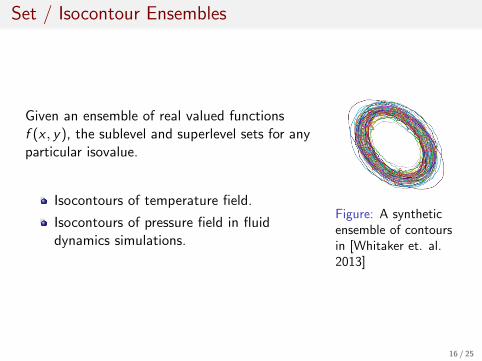
Set / Isocontour Ensembles

Given an ensemble of real valued functionsf (x , y), the sublevel and superlevel sets for anyparticular isovalue.

Isocontours of temperature field.

Isocontours of pressure field in fluiddynamics simulations.

Figure: A syntheticensemble of contoursin [Whitaker et. al.2013]

16 / 25

Data Depth Formulation for Sets

Figure: Examples of set band [Whitaker et. al. 2013]

Set band formulation:

S ∈ sB(S1, . . . ,Dj)↔j⋃

k=1

Sk ⊂ S ⊂j⋂

k=1

Sk (5)

Set band depth formulation:

sBDj (S) = P (S ⊂ sB(S1, . . . ,Sj) (6)

17 / 25

Visualization of Data Depth for Sets

(a)

(b)

Figure: Contour boxplot for an ensemble of isocontours of pressure field[Whitaker et. al. 2013]

18 / 25

Paths (on a graph)

Let G = {V ,E ,W }. A path p can be denotedas p : I 7→ V where index set I = (1, . . . ,m)

Paths of packets in computer networks.

Paths on transportation networksmodelled as graphs.

Figure: A syntheticensemble of paths ona graph.

19 / 25

Data Depth Formulation for Paths

Figure: Illustration of band formed by 3 paths.

Path band formulation:

p ∈ B[Pj ] iff p(l) ∈ H[p1(l), . . . , pj(l)] ∀l ∈ I (7)

Path band depth formulation:

pBDj (p) = E [χ(p ∈ B(pj))] (8)

20 / 25

Visualization of Data Depth for Paths

(a) (b)

Figure: Path boxplots for paths on AS and road graphs.

21 / 25

Outline

1 Data Depth BackgroundWhat is Data Depth?Geometrical Data DepthGeneral Properties of Data Depth

2 Generalized Notions of Data DepthFunctionsMultivariate CurvesSetsPaths (on a graph)

3 DiscussionRelaxed FormulationsAdvantages and Limitations of Data Depth

22 / 25

Relaxed formulations

1 Modified Band Depth - Instead of an indicator function,measure object inside the band.

2 ε Subsets - Indicator function with a relaxed threshold.

23 / 25

Advantages and Limitations

For Combinatorial Data Depth Formulations for Complex Data

Advantages

No assumption required for the underlying distribution.

Captures nonlocal relationships

Robust.

Limitations

Computationally expensive for large ensembles.

24 / 25

Thank You

Questions?

25 / 25