Leitenstorfer, Tutz:

Generalized Monotonic Regression Based on B-Splineswith an Application to Air Pollution Data

Sonderforschungsbereich 386, Paper 444 (2005)

Online unter: http://epub.ub.uni-muenchen.de/

Projektpartner

Generalized Monotonic Regression Based onB-Splines with an Application to Air Pollution

Data

Florian Leitenstorfer, Gerhard TutzLudwig-Maximilians-Universitat Munchen

Akademiestraße 1, 80799 Munchen

{leiten,tutz}@stat.uni-muenchen.de

30th May 2005

Abstract

In many studies where it is known that one or more of the certaincovariates have monotonic effect on the response variable, common fittingmethods for generalized additive models (GAM) may be affected by asparse design and often generate implausible results. A fitting procedure isproposed that incorporates the monotonicity assumptions on one or moresmooth components within a GAM framework. The flexible likelihoodbased boosting algorithm uses the monotonicity restriction for B-splinecoefficients and provides componentwise selection of smooth components.Stopping criteria and approximate pointwise confidence bands are derived.The method is applied to data from a study conducted in the metropolitanarea of Sao Paulo, Brazil, where the influence of several air pollutants likeSO2 on respiratory mortality of children is investigated.

Keywords: Monotonic regression, Generalized additive models, Likelihoodbased boosting, Air pollution data

1 Introduction

In many biometrical problems where generalized smooth regression methods areused, a monotonic relationship between one or more explanatory variables andthe response variable is to be assumed. A typical problem of this type which willbe considered more closely arises in studies where the influence of air pollutionon mortality or illness is investigated, see e.g. Schwartz (1994) or Conceicao,Miraglia, Kishi, Saldiva & Singer (2001). In these analyses, an increase of deaths

1

or cases of illness is expected with an increasing concentration of a certain pol-lutant. When standard smoothing techniques, like spline smoothing (Green &Silverman 1994) or local polynomial fitting (Fan & Gijbels 1996), are applied todata of this type in a generalized additive modeling approach, the fitted curvesare often affected by few data points. This may lead to unconvincing results.In the following, it is proposed to incorporate the knowledge about monotonicrelationships in the estimation by using monotonic regression methods.

Starting from the Pool Adjacent Violators Algorithm (PAVA) (see e.g. Robert-son, Wright & Dykstra 1988) which produces a step function, a variety of methodshas been developed to smooth the PAVA results, obtaining a smooth estimate ofthe underlying monotonic function. Details of such approaches, which are mainlybased on kernel regression techniques, are given in Friedman & Tibshirani (1984),Mukerjee (1988) or Mammen, Marron, Turlach & Wand (2001). Alternative ap-proaches, which will be pursued in the following, are based on the expansion ofa monotonic function into a sum of basis functions, i.e. f =

∑j αjBj. To as-

sure monotonicity of the estimate, adequate constraints have to be put on thecoefficients αj. Ramsay (1988) suggests the use of monotonic basis functions(integrated splines), while Kelly & Rice (1991) propose a B-spline basis. Asthe B-spline approach has become very popular in nonparametric regression (seeEilers & Marx 1996), we will focus on the latter.

Most of the publications on monotonic regression are limited to unidimen-sional smoothing problems with a Gaussian response variable y. In the exampleconsidered here, as in many ecological or biometrical applications, one has multi-ple covariates x′ = (x1, . . . , xp), and only for some of the covariates a monotonicrelationship to E(y|x) has to be assumed. Furthermore, the response variablesare typically binary or count data, which are considered as binomial or Poissondistributed. Because little work has been done on monotonic regression in a gen-eralized linear model (GLM) context, least squares approaches have often beenused in such cases (see e.g. Kelly & Rice 1991), which lead to dissatisfactoryresults. Flexible modeling tools are needed, where monotonicity restrictions caneasily be incorporated into a generalized additive model (GAM) framework.

Recently, boosting approaches became increasingly important in nonpara-metric regression, see e.g. Buhlmann & Yu (2003). As Tutz & Leitenstorfer(2005) demonstrate, monotonicity restrictions are easy to include in likelihoodbased algorithms for generalized response problems by componentwise boost-ing of monotonic basis functions in each step. In the present paper we suggestboosting based on B-spline basis functions, rather than using monotonic basisfunctions as in Tutz & Leitenstorfer (2005) or Ramsay (1988). When using B-splines, the monotonicity condition of the estimate is preserved in a different way.A special update scheme for the basis coefficients is proposed which shows goodperformance. It should be noted that the proposed method avoids the use ofalgorithms which handle inequality constraints. Procedures of this type typicallyimply heavy computational burden and often yield unstable estimates. From

2

a Bayesian perspective, a B-spline approach to monotonic regression has beensuggested by Brezger & Steiner (2004).

0 20 40 60 80

02

46

810

12

Concentration of S02

respirato

ry d

eath

s

0 20 40 60 80

02

46

810

12

0 20 40 60 80

02

46

810

12

0 20 40 60 80

02

46

810

12

GAMGMBBoost, AICGMBBoost, BIC

0 50 100 150 200

02

46

810

12

Concentration of PM10

respirato

ry d

eath

s

0 50 100 150 200

02

46

810

12

0 50 100 150 200

02

46

810

12

0 50 100 150 200

02

46

810

12

GAMGMBBoost, AICGMBBoost, BIC

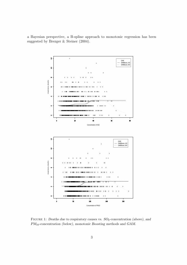
Figure 1: Deaths due to respiratory causes vs. SO2-concentration (above), and

PM10-concentration (below), monotonic Boosting methods and GAM.

3

We illustrate generalized monotonic regression techniques on a data set thathas been previously analyzed by Conceicao, Miraglia, Kishi, Saldiva & Singer(2001), Singer, Andre, Lima & Conceicao (2002) and Einbeck, Andre & Singer(2004). The data have been collected to evaluate the association between mor-tality of children under five due to respiratory causes and the concentration ofvarious air pollutants in the city of Sao Paulo, Brazil, form 1994 to 1997 (the dataare available at http://www.ime.usp.br/∼jmsinger; a detailed description followsin Section 4). In Figure 1, in each panel the number of daily respiratory deathsis given as a function of a specific air pollutant, fitted by the proposed monotonicmethods and a unconstrained generalized smoothing method (function gam() ofthe R library mgcv). The response variable was assumed to be Poisson distrib-uted, and the log-link was used. These examples show that especially for SO2

and PM10, the GAM fit is pulled downwards by few observations on the right sidewhere the design is sparse. The fitted curves imply a decrease of the mortalityfor high pollutant concentrations, which has no causal plausibility. In contrast,the monotonic approach shows resistance against such inconsistencies and yieldsreliable fits. Einbeck, Andre & Singer (2004) found the same problems with thedata and proposed to stabilize a local fitting procedure by downweighting pointswith small design density.

In Section 2 the concept of monotonic likelihood boosting based on B-splinesis introduced, and an extension to multiple covariate settings is given. In Section3 approximate pointwise confidence bands are derived. In section 4 we take acloser look on the data set mentioned above. Note that throughout the paper,we refer to monotonic regression as nondecreasing regression.

2 Boosting B-splines in generalized monotonic regression

2.1 Monotonicity constraints for B-splines

First, we consider a generalized smooth monotonic regression problem with de-pendent variable y that can be non-Gaussian, and a single covariate x. As ingeneralized linear models (e.g. McCullagh & Nelder 1989) it is assumed thatyi|xi has a distribution from a simple exponential family f(yi|xi) = exp{(yiθi −b(θi))/φ+ c(yi, φ)} where θi is the canonical parameter and φ denotes the disper-sion parameter. The link between µi = E(yi|xi) and the explanatory variable xi

is determined by µi = h(ηi), where h is a given response function which is strictlymonotone (the inverse of the link function g = h−1), and the predictor ηi = η(xi)is a function of x. While in generalized linear models, η(x) is assumed to be alinear predictor, here more generally it is assumed that η(x) = f(x) is a smoothfunction that satisfies the monotonicity condition

f(x) ≥ f(z) if x > z. (1)

Obviously, monotonicity in η transforms into monotonicity in the means.

4

Due to their flexibility, smoothing methods based on B-splines are a commontool in statistics, see e.g. Eilers & Marx (1996). Such approaches are based onan expansion of f into B-spline basis functions, where a sequence of knots {tj} isplaced equidistantly within the range [xmin, xmax]. With m denoting the numberof interior knots, one obtains the linear term

η(x) = α0 +m∑

j=1

αjBj(x, q), (2)

where q denotes the degree of the B-splines and m = m + 1 + q (the augmentedset of knots). An algorithm for the computation of B-splines of degree q is givenin De Boor (1978). Monotonicity can be assured in the following way: supposewe have B-splines of degree q ≥ 1 and let h be the distance between the equallyspaced knots. Then the derivative η′(x) = ∂η(x)/∂x can be written as

η′(x) =∑

j

αjB′j(x, q) =

1

h

∑j

(αj+1 − αj)Bj(x, q − 1),

for a proof see De Boor (1978). Since Bj(x, q − 1) ≥ 0, it follows from

αj+1 ≥ αj, (3)

that η′(x) ≥ 0 holds. In other words, since (3) is a sufficient condition for themonotonicity of η(x), the sequence of coefficients αj has to be nondecreasingin order to obtain monotonic functions. This property of B-splines has beenpreviously exploited by Kelly & Rice (1991) and Brezger & Steiner (2004) in amonotonic regression setting.

2.2 An outline of the algorithm

Boosting has originally been introduced within the machine learning community(e.g. Schapire 1990) for classification problems. More recently, the approachhas been extended to regression modeling with a continuous dependent variable(e.g. Buhlmann & Yu 2003, Buhlmann 2004). The basic idea is to fit a functioniteratively by fitting in each stage a ”weak” learner to the current residual. Incomponentwise boosting as proposed by Buhlmann & Yu (2003), only the contri-bution of one variable is updated in one step. In contrast to these approaches wepropose to update a specific simplification of the predictor which makes it easyto control the monotonicity restriction.

For simplicity, in the following, the degree q of the B-splines is suppressed. Inmatrix notation, the data are given by y = (y1, . . . , yn)′, x = (x1, . . . , xn)′. Basedon the expansion into basis function, the data set may be collected in matrixform (y,B), where B = (B1(x), . . . , Bm(x)), Bj(x) = (Bj(x1), . . . , Bj(xn))′.

5

The residual model that is fitted by weak learners in one iteration step usesa grouping of B-splines. One considers for r = 1, . . . ,m− 1 the simplified modelthat has the predictor

η(xi) = α0(r) + α1(r)

(r∑

j=1

Bj(xi)

)+ α2(r)

(m∑

j=r+1

Bj(xi)

). (4)

When fitting model (4) the monotonicity constraint is easily checked by compar-ing the estimates α1(r) and α2(r), since monotonicity follows from α2(r) ≥ α1(r).Given an estimate from previous fitting,

ηold(xi) = α0,old +m∑

j=1

αj,oldBj(xi)

refitting is performed by

ηnew(xi) = ηold(xi) + α0(r) + α1(r)

(r∑

j=1

Bj(xi)

)+ α2(r)

(m∑

j=r+1

Bj(xi)

)

= α0,old + α0(r) +r∑

j=1

(αj,old + α1(r))Bj(xi) +m∑

j=r+1

(αj,old + α2(r))Bj(xi).

It is obvious that ηnew is monotonic if estimates fulfill α2(r) ≥ α1(r), providedthat the previous estimate ηold was monotonic. The grouping of basis functionsinto B1, . . . , Br and Br+1, . . . , Bm which are adapted by the amount α1(r) in thefirst and α2(r) in the second group allows to control monotonicity in a simpleway. Fitting a full model with m new parameters would imply much more com-putational effort and rise problems if the newly fitted model is non-monotonic.Instead, the possible groupings (r = 1, . . . , m−1) are evaluated and in analogy tocomponentwise boosting the best refit is selected. The grouping of B-splines canbe derived as a restricted model in the sense of restricted least squares estimators(RLSE) in linear models, see Theil & Goldberger (1961). In the usual form of asmoothed estimate based on B-splines, model (4) is given by

η(xi) = α0(r) +r∑

j=1

α(r)j Bj(xi) +

m∑j=r+1

α(r)j Bj(xi) (5)

with the constraints α(r)1 = · · · = α

(r)r = α1(r), α

(r)r+1 = · · · = α

(r)m = α2(r). The

constraints specify that blocks of r and m− r parameters have to be identical.Before giving the algorithm, which is based on likelihood based boosting

strategies as proposed by Tutz & Binder (2004), the fit of model (4) is embeddedinto the framework of penalized likelihood estimation. Let

R(r) =

(1r 0r

0m−r 1m−r

),

6

with 0r, 1r denoting the vectors of length r containing 0s and 1s only, then (4)may be represented in matrix form by the linear predictor η(x) = B(r)ααα(r), whereB(r) = (1,BR(r)) and ααα(r) = (α0(r), α1(r), α2(r))

′. It is proposed that in eachboosting step, model (4) is estimated by one-step Fisher scoring based on gen-eralized ridge regression (Marx, Eilers & Smith 1992). Common ridge regressionmaximizes the penalized log-likelihood

lp(ααα(r)) =n∑

i=1

li(ααα(r))− P (ααα(r)),

where li(ααα(r)) = li(h(B(r)ααα(r))) is the usual log-likelihood contribution of theith observation and the P (ααα(r)) = (λ/2)ααα′(r)ααα(r) represents the penalty term with

ridge parameter λ. However, model (4) is asymmetric in a specific sense. Considertherefore the representation (5) of the restricted problem. If for example r = 2,

the first constraint α(2)1 = α

(2)2 concerns only two parameters, whereas the second

constraint α(2)3 = · · · = α

(2)m concerns m − 2 parameters, which for m = 20

means 18 parameters are restricted. It seems sensible to adapt the penalty to thecomplexity of the constraints which are implicitly used. We propose to use thepenalty

P (ααα(r)) =λ

2(rα1(r) + (m− r)α2(r)), (6)

where the parameters are weighted by the number of parameters that are implic-itly considered as identical. When using (6) we found much better performanceof the estimator than by using the usual ridge constraint P (ααα(r)) = (λ/2)ααα′(r)ααα(r).In matrix form one obtains the penalized log-likelihood

lp(ααα(r)) =n∑

i=1

li(ααα(r))− λ

2ααα′(r)ΛΛΛααα(r),

where

ΛΛΛ =

(0 00 R′

(r)R(r)

)= diag(0, r,m− r), (7)

and λ > 0 represents the ridge parameter. Derivation yields the correspondingpenalized score function

sp(ααα(r)) =∂lp(ααα(r))

∂ααα(r)

= B′(r)W(ηηη)D(ηηη)−1(y − h(ηηη))− λΛΛΛααα(r), (8)

with W(ηηη) = D2(ηηη)ΣΣΣ(ηηη)−1, D(ηηη) = diag{∂h(η1)/∂η, . . . , ∂h(ηn)/∂η}, ΣΣΣ(ηηη) =diag{σ2

1, . . . , σ2n}, σ2

i = var(yi), all of them evaluated at the current value of η.Note that the intercept term is refitted in each iteration by the correspondingunpenalized one-step estimate. The monotonicity constraint from (3) is incor-porated by taking into account only estimates which fulfill α2(r) > α1(r). It is

7

easily seen that the update scheme given below yields the desired nondecreasingsequences of estimates α1, . . . , αm in each boosting iteration. An outline of thealgorithm is as follows.

Monotonic Likelihood Boosting for B-splines

Step 1 (Initialization)

Standardize y to zero mean, i.e. set α0 = y, ααα(0) = (y, 0, . . . , 0)′, ηηη(0) =(y, . . . , y)′ and µµµ(0) = (h(y), . . . , h(y))′.

Step 2 (Iteration)

For l = 1, 2, . . .

1. Fitting stepFor r = 1, . . . ,m − 1 compute the modified ridge estimate based on onestep Fisher scoring,

ααα(r) = (B′(r)WlB(r) + λΛΛΛ)−1B′

(r)WlDl−1(y − µµµ(l−1)), (9)

where ααα(r) = (α0(r), α1(r), α2(r))′, Wl = W(ηηη(l−1)), Dl = D(ηηη(l−1)), and

µµµ(l−1) = h(ηηη(l−1)). Compute the potential update of the linear predictor,ηηηr,new = ηηη(l−1) + B(r)ααα(r). Let A = {r : α1(r) < α2(r)} denote the candidatesthat fulfill the monotonicity constraint.

2. Selection stepCompute the potential update of the linear predictor, ηηη(r),new = ηηη(l−1) +B(r)ααα(r), r ∈ 1, . . . , m− 1. Choose rl ∈ A such that the deviance is mini-mized, i.e.

rl = arg minr∈A

Dev(ηηη(r),new).

3. UpdateSet

α(l)0 = α

(l−1)0 + α0(rl),

α(l)j =

{α

(l−1)j + α1(rl) 1 ≤ j ≤ rl

α(l−1)j + α2(rl) j > rl,

(10)

ηηη(l) = ηηη(l−1) + B(rl)ααα(rl) and µµµ(l) = h(ηηη(l)).

8

When using boosting techniques, the number of iterations l plays the roleof a smoothing parameter. Therefore, in order to prevent overfitting, a stop-ping criterion is necessary. A quite common measure of the complexity of asmooth regression fit is the hat-matrix. Consequently, Buhlmann & Yu (2003)and Buhlmann (2004) developed a hat-matrix for L2-boosting with continuous de-pendent variable. In the case of likelihood boosting, for more general exponentialtype distributions, the hat-matrix has to be approximated. For integrated splines,Tutz & Leitenstorfer (2005) give an approximation based on first order Taylorexpansions, which shows satisfying properties. It is straightforward to derive thehat-matrix for the present case along the lines of Tutz & Leitenstorfer (2005).

With M0 = 1n1n1

′n and Ml = ΣΣΣ

1/2l W

1/2l B(rl)(B

′(rl)

WlB(rl) +λΛΛΛ)−1B′(rl)

W1/2l ΣΣΣ

1/2l ,

where Wl = W(ηηη(l−1)), l = 1, 2, . . . , and ΣΣΣl = ΣΣΣ(ηηη(l−1)), the approximate hat-matrix is given by

Hl = I− (I−M0)(I−M1) · · · (I−Ml) =l∑

j=0

Mj

j−1∏i=0

(I−Mi), (11)

with µµµ(l) ≈ Hly. By considering tr(Hl) as the degrees of freedom of the smoother,we investigate the AIC and the BIC criteria as potential stopping criteria,

AIC(l) = Devl + 2tr(Hl)

andBIC(l) = Devl + log(n)tr(Hl),

where Devl = 2∑n

i=1[li(yi) − li(η(l)i )] denotes the deviance of the model in the

lth boosting step. The optimal number of boosting iterations is defined bylAICopt = arg minl AIC(l) or lBIC

opt = arg minl BIC(l). Since the BIC (Schwarz1978) penalizes the complexity of the fit stronger, usually more sparse modelsresult. A more extensive treatment of stopping criteria for boosting algorithmsis given in Buhlmann & Yu (2005).

2.3 Extension to generalized additive models

In biometrical or ecological problems, one is usually interested in the effect ofseveral predictor variables, where some of them might have monotonic influenceon y, whereas others have not. Additionally, a smooth estimation is not alwaysappropriate for all covariates. In the following we demonstrate that the conceptgiven above can easily be extended to a GAM setting (see e.g. Hastie & Tibshirani1990 or Marx & Eilers 1998). Let

η(x) = α0 +

p∑s=1

fs(xs), (12)

9

where for part of the unknown smooth functions (say f1, . . . , fv, v ≤ s) monotonic-ity constraints are assumed to hold. Using the matrix notation from above, wehave a design matrix X = (x1, . . . ,xp), where xs = (x1s, . . . , xns)

′. Component-wise expansion into B-spline basis functions leads to the data set (y,B(1), . . . ,B(p)),where B(j) refers to the jth predictor.

It is essential to distinguish between components that are under monotonicityrestrictions and those that are not. For the former, grouping of basis functionsis done within each component in the same way as described in (4). For theunconstrained components, we follow Buhlmann & Yu (2003) and Tutz & Binder(2004) and use penalized regression splines (P-splines, cf. Eilers & Marx 1996) asweak learner for the chosen component. Thereby, the second order differences ofthe B-spline coefficients are penalized. For simplicity, it is assumed that the samenumber of basis functions m is used for all fs. The vector of basis coefficientsfor the whole model is then given by ααα = (α0, α1,1, . . . , α1,m, . . . , αp,1, . . . , αp,m)′.Thus, step 2 (iteration) of the algorithm described above is extended as follows:

Step 2 (Iteration):For l = 1, 2, . . .

1. Fitting stepFor s = 1, . . . , p,

• If s ∈ {1, . . . , v} (the components under monotonicity constraint),compute the estimates from (9) componentwise for the possible group-ings r = 1, . . . , m− 1, with

B(s)(r) = (1,B(s)R(r)). (13)

The set of indices for components s and split points r that satisfy themonotonicity constraint is given by

A1 = {(s, r) ∈ {1, . . . , v} × {1, . . . , (m− 1)} : α(s)1(r) < α

(s)2(r)}.

• If s ∈ {v + 1, . . . , p} (the components without constraints), computethe one step Fisher scoring estimate of the P-spline including the in-tercept term,

ααα(s) = (B∗(s)′WlB∗(s) + λP∆∆∆′

2∆∆∆2)−1B∗(s)′WlDl

−1(y − µµµ(l−1)), (14)

where

∆∆∆2 =

0 1 −2 1...

. . . . . . . . .

0 . . . 1 −2 1

denotes the matrix representation of the second order differences, andB∗(s) = (1,B(s)). Since the P-spline fit (14) does not distinguish be-tween split points r ∈ {1, . . . , m−1}, for convenience of notation we set

10

r = 0 and extend the selection set by A2 = {(s, 0), s ∈ {v +1, . . . , p}},yielding

A = A1 ∪ A2. (15)

2. Selection stepCompute the potential update of the linear predictor, which only for themonotonic coefficients s ≤ v depends on the split point r. Otherwise, r isset to 0, indicating that ηηη

(s)(0),new is not affected by r. Choose (sl, rl) ∈ A

such that the deviance is minimized, i.e.

(sl, rl) = arg min(s,r)∈A

Dev(ηηη(s)(r),new).

3. UpdateBesides the intercept, in each iteration only the basis coefficients belongingthe chosen component sl are refitted. That means, if the selected sl is in{1, . . . , v}, then α

(l)0 and α

(l)sl,j

, j = 1, . . . , m, are updated by the refittingscheme (10). If sl > v, then update

α(l)0 = α

(l−1)0 + α

(sl)0 and α

(l)sl,j

= α(l−1)sl,j

+ α(sl)j ,

with ααα(sl) from (14).

By using B(s)(r) from (13), along with B∗(s) and the penalty matrix ∆∆∆′

2∆∆∆2 for

the P-spline estimates, the hat-matrix approximation from (11) and the corre-sponding AIC and BIC stopping criteria can be extended to the additive setting.In the case of many predictors it might occur that boosting stops before a certaincomponent has been chosen. Thus, the extended approach has the nice effect ofdoing variable selection for smooth components, similar to the methods proposedby Buhlmann & Yu (2003). This additional strength is important only in datasets with a large number p of covariates, where only some of them are influential.

If a set of covariates xw+1, . . . , xp, v ≤ w < p has to be modeled in a parametricway, i.e. if we have a semiparametric linear predictor

η(x) = α0 +w∑

s=1

fs(xs) +

p∑u=w+1

βuxu

(e.g. Speckman 1988), the estimation of the corresponding parameters is easy toincorporate in our proposed algorithm. However, it turns out that fixed effectsthat are included with one basis function in the selection are rarely chosen, espe-cially for dummy covariates, since they carry much less information compared tometrical variables. Hence, after initialization, we treat parametric covariates likethe intercept: unpenalized one step estimates result from (9) and (14) respec-

tively by simply enlarging the matrix B(s)(r) (B∗(s)) by xw+1, . . . ,xp and correcting

the penalty matrix ΛΛΛ (∆∆∆′2∆∆∆2) appropriately. The corresponding coefficients are

then updated in each boosting iteration.

11

3 Standard deviations

In order to obtain standard deviations for function estimates, we suggest to startfrom the approximate hat-matrix given in (11). Consider the model from (12),where components 1, . . . , v are estimated under the monotonicity constraint andcomponents v +1, . . . , p are not, the linear predictor after l boosting iterations isgiven by

ηηη(l) = 1nα(l)0 +

p∑s=1

B(s)ααα(l)s , (16)

where ααα(l)s = (α

(l)s,1, . . . , α

(l)s,m)′ and α

(l)0 results from updating the intercept in each

iteration. Let sk be the component chosen in the kth boosting iteration, one hasfrom the update step of the extended algorithm,

B(s)ααα(k)s =

{B(s)ααα(k−1)

s , sk 6= s

B(s)ααα(k−1)s + Sk(y − µµµ(k−1)), sk = s,

(17)

where, according to (12) and (14),

Sk =

{B

(sk)(rk)(B

(sk)(rk)

′WkB(sk)(rk) + λΛΛΛ)−1B

(sk)(rk)

′WkDk−1, sk ≤ v

B∗(sk)(B∗(sk)′WkB∗(sk) + λP∆∆∆′

2∆∆∆2)−1B∗(sk)′WkDk

−1, sk > v.(18)

From (18), it becomes apparent that the type of the update of the chosen com-ponent depends on the presence or absence of a monotonicity restriction. Usingthe indicator function I(.), (17) can be written in the closed form

B(s)ααα(k)s = B(s)ααα(k−1)

s + I(sk = s)Sk(y − µµµ(k−1)).

With the approximation of the hat-matrix, one has µµµ(k−1) ≈ Hk−1y, which leadsto

B(s)ααα(k)s ≈ B(s)ααα(k−1)

s + I(sk = s)Sk(I−Hk−1)y,

and hence, in a recursive fashion,

B(s)ααα(l)s ≈ Q

(s)l ,

where

Ql =l∑

k=1

I(sk = s)Sk(I−Hk−1).

Approximate confidence intervals for the estimate of the smooth component fs

after l boosting iterations are then found from

cov(Q(s)l y) = Q

(s)l cov(y)Q

(s)l′,

where cov(y) = diag(σ21, . . . , σ

2n).

12

4 Air pollution in Sao Paulo

In the following the air pollution data from Section 1 are investigated more closely.The objective is to evaluate the association between mortality of children underfive attributed to respiratory causes and the concentration of SO2, CO, PM10 andO3. The response variable is the number of daily deaths attributed to respiratorycauses in the city of Sao Paulo. The sample size is n = 1067. A standardapproach for data of this type is to use a generalized additive ’core’ model whichincludes terms to control for trend, seasonality and other influential variableslike temperature or humidity, cf. Schwartz (1994). As the dependent variableconsists of count data, we use a Poisson model along with the (natural) log-link,and consider the core model of Singer, Andre, Lima & Conceicao (2002),

η = log[E(resp. deaths)] = α0 + f1(time) + f2(temp) + f3(humidity)

+β1 ·Monday + · · ·+ β6 · Saturday (19)

+β7 · non-resp. deaths.

The model includes non-specified functions to control for long-term seasonality(days), temperature (daily minimum, lag 2) and relative humidity (lag 0). In ad-dition day of week dummies are included to control for short-term seasonality andthe number of deaths by non-respiratory causes as a linear term. The basic strat-egy to investigate the effect of a specific pollutant is to take only this pollutantinto the model. In the following, we will exemplarily focus on the concentrationof SO2, given in daily 24-h mean values of µg/m3, considering the predictor

η = η + f4(SO2). (20)

Since an increase in respiratory mortality with rising pollutant concentrations isexpected, it is sensible to assume the function f4 to be isotonic. To account forthat assumption, model (20) has been fitted by the boosting procedure describedin Section 2 (GMBBoost, Generalized Monotonic B-spline Boosting), where f4

was estimated under the monotonicity constraint. We used a B-spline basis ofdegree 3 with m = 20 equidistant interior knots for each of the smooth compo-nents. The penalty parameter λP in the one step P-spline estimates from (14)for the non-monotonic components was set to 200. For the monotonic estima-tion of f4, we chose a smaller λ of 20 due to the multiplication by weighting thepenalty, see (6). It should be noted that the choice of penalty parameters is notcrucial in boosting approaches; it is chosen for convenience such that the numberof iterations is not too high. The fixed effects were re-estimated in each iteration.To stabilize the approximation of the hat-matrix, we put an additional shrinkagefactor of ν = 0.1 on the estimates in each boosting step. Boosting was stoppedby AIC as well as by BIC. For comparison, we also fitted a generalized additivemodel using gam() from the R package mgcv (for details see R Foundation forStatistical Computing 2004 and Wood 2000).

13

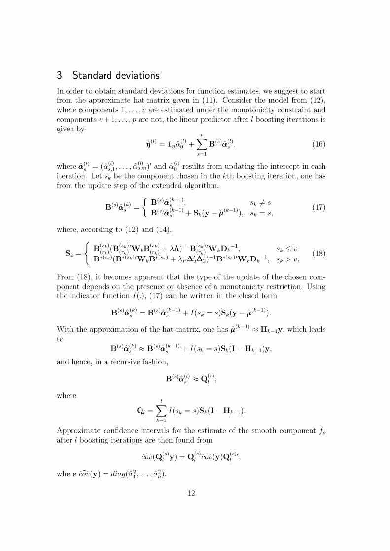
Figure 2 shows the estimated curves f1, . . . , f4 for the various fitting proce-dures. It is seen from f1 (upper left panel) that the seasonal pattern in mortalityis evident for all three fitting methods. Mortality tends to decrease as temper-ature increases (upper right panel). Interestingly, the GAM fit yields a almoststraight line, while both boosting estimates show a plateau between 10 and 15◦C, a result that has also been reported by Conceicao, Miraglia, Kishi, Saldiva& Singer (2001). For the relative humidity (lower left panel), GAM results in anincreasing, again almost straight line. AIC-stopped boosting shows two troughsat 65% and 90% relative humidity, while BIC-stopped boosting assigns only amarginal relevance to that component. The most interesting result is found inthe fit for the concentration of SO2 (lower right panel), where the monotonicityconstraint is set in GMBBoost. The GAM fit shows the same effect that is seenin the simple introductory example presented in Figure 1: the curve is severelypulled down by the sparse points of high concentrations, resulting in the implau-sible result of decreasing mortality for concentrations larger than 40 µg/m3. Thisphenomenon has been also detected by Einbeck, Andre & Singer (2004). Instead,GMBBoost shows a quite different behaviour. Since monotonicity is assumed forthis component, one obtains a monotonic increasing fit, which remains constanton a high level of mortality for high pollutant concentrations. This result is inaccordance with biological theory. For BIC-stopped boosting, the effect is flatterthen for AIC-stopped boosting.

In Table 1, the parameter estimates for the fixed effects, controlling for long-term seasonality and non-respiratory deaths, are given for the different fittingmethods, along with the corresponding values of AIC and BIC. It is seen thatthe estimates are rather stable across fitting procedures. More importantly, itis seen that AIC-stopped GMBBoost outperforms GAM distinctly in terms ofthe AIC criterion, indicating that the constrained boosting approach results ina more appropriate model for the present data. Interestingly, also BIC-stoppedboosting does slightly better than GAM in terms of AIC. A similar result isseen for the BIC. The corresponding GMBBoost estimate performs best for thiscriterion, whereas GAM does even worse than AIC-stopped boosting. Since inthe BIC criterion, the complexity of the fit is penalized stronger as comparedto AIC, GMBBoost stops earlier for the former (lBIC

opt = 88) than for the latter(lAIC

opt = 213).Figure 3 shows the curves fitted by AIC-stopped GMBBoost, and approximate

0.95 pointwise confidence bands as derived in Section 3. In the lights of confidenceintervals, it is seen that the effects of temperature and humidity are rather weak.

In studies of the type presented here, one is often interested in the risk ofdeath at a certain pollutant concentration, relative to the risk of death at the min-imum concentration of that pollutant, see e.g. Singer, Andre, Lima & Conceicao(2002) or Einbeck, Andre & Singer (2004). Let SO2(i) be the recorded concentra-tion in observation i, i = 1, . . . , 1067, and SO2(min) the minimum concentration

14

0 500 1000 1500

−0.

6−

0.2

0.2

0.4

0.6

number of days

eta

cont

rib.

||||||||||||||||||||||||||||||||||||||||||||||||||||||||||||||||||||||||||||||||||||||||||||||||||||||||||||||||||||||||||||||||||| |||||||||||||||||||||||||||||||||||||||||||||||||||||||||||||||||||||||||| |||||||||||||||||||||||||||||||||||||||||||||||||||||||||||||||||||||||||||||| |||| |||||||||||||||||||||||||||||||||||||||||||||||||||||||||||||||||||||||||||||||||||||||||||||||||||||||||||||||||||||||||||||||||||||||||||||||||||||||||||||||||||||||||||||||||| ||||||||||||||||||||||||||||||||||||||||||||||||||||||||||||||||||||||||||||||||||||||||||||||||||||||||||||||||||||||||||||||||||||||||||||||||||||||||||||||||||||||||||||||||||||||||||||||||||||||||||||||||||||||||||||||||||||||||||||||||||||||||||||||||||||||||||||||||||||||||||||||||||||||||||||||||||||||||||||||||||||||||||||||||||||||||||||||||||||||||||||||||||||||||||||||||||||||||||||||||||||||||||||||||||||||||||||||||||||||||||||||||||||||||||||||||||||||||||||||||||||||||||||||||||||||||||||||||||||||||||||||||||||||||||||||||||||||||||||||||||||||||||||||||||||||||||||||||||||||||||

0 500 1000 1500

−0.

6−

0.2

0.2

0.4

0.6

number of days

eta

cont

rib.

0 500 1000 1500

−0.

6−

0.2

0.2

0.4

0.6

number of days

eta

cont

rib.

0 500 1000 1500

−0.

6−

0.2

0.2

0.4

0.6

number of days

eta

cont

rib.

0 5 10 15 20

−0.

4−

0.2

0.0

0.2

min. temperature

eta

cont

rib.

|| ||| |||| | ||| || | || || | | | || | ||||| || |||| | ||| | | ||| ||| | | || || ||||| ||| | || ||| ||| | ||| | ||||| | ||||| ||||| | | | |||| | || | ||| ||||| | | || | | ||||||| || ||||| | | | | ||||| ||| || ||| || ||| | || ||| | ||| || | || || ||| | | |||| | | | || | ||| ||| ||| | | | | |||||| | |||||| || ||||| | | ||| | |||| ||| | || || ||||| | || | | | |||| || | | || | ||| | || |||| | ||| | | ||||| | | |||| || | | || || |||| | | || || ||| | || || |||| | |||| ||||| | || | ||||| || || | |||| || ||| ||||| | ||||| ||| || | | || ||| ||| ||| | |||| ||| |||| || | | || |||| | | || || | | | || || ||| |||| | | ||||| ||||| | |||| | | | || || | | |||||| || |||||| | ||| ||||| || |||| | | | |||| | | |||||| ||| | ||| || ||| |||| | | || | || |||| |||||||| | ||| || ||| | | ||||| ||| || | | ||||||| | ||| | | | || | |||| || || | ||| || | || | ||| ||||| |||| | | ||||| | | | | | | |||| ||| | || | || | | | | ||||| | | ||||||| |||| || || |||| | || ||| | || ||||||||| | || | | || | | || | |||| | | ||| | ||| |||| || | | ||||||| || | ||| ||| ||||| || ||||||| ||| |||| || || || | || | ||| || || || ||| |||| || || || || |||||||| | ||| | | | ||| || | | ||||||| || | || || | ||||||| || || || |||| |||| || |||| ||| || || | || ||| | |||||| | | |||| | || || ||||| || | || || ||| ||| | ||| | ||||| | ||| | || |||| |||| || | | ||| | || | |||| || | || || | ||| | |||| || | | || | | | || || |||| | ||| || | |||| |||| || | |||| ||| | | | || | ||||| | | || | | ||| | ||||| || || ||| | || ||| | |||| | | |||| ||| | | || || | |||| | | || ||| | | | || |||| |||

0 5 10 15 20

−0.

4−

0.2

0.0

0.2

min. temperature

eta

cont

rib.

0 5 10 15 20

−0.

4−

0.2

0.0

0.2

min. temperature

eta

cont

rib.

0 5 10 15 20

−0.

4−

0.2

0.0

0.2

min. temperature

eta

cont

rib.

50 60 70 80 90 100

−0.

20−

0.10

0.00

0.10

relative humidity

eta

cont

rib.

|| ||| || | |||| || | || ||||| |||||| | || | |||| | | |||| | |||| || |||| | | ||| | |||| |||||| ||| || || ||| || | |||||| | |||| | | |||| | ||| | ||| ||||| | | || | || | || ||| | | |||||| | || ||| || |||||||| ||| | | | | | ||| || || |||| ||| | |||||| | ||| | || || || | | ||||||| | |||||| || | | |||| ||| |||| | || | | |||| || | ||| | |||||| ||| | ||| |||| | | || |||| | || ||| | ||| | ||| | ||| | | || ||||| | | ||| |||| | || | | | |||| |||| ||| || || ||| | || ||| | |||| ||| | ||| | ||||| | | ||||| || || | || || | ||| || |||| | || |||||| |||| | ||| |||| | |||| || ||| ||| ||||| | | ||| |||| || || || | |||||| | | || ||||||| || | | | || | || ||| | | | |||| || ||| || |||| | | || |||| || ||| || ||| | |||| || ||| ||| ||||| | || | | ||| | || |||| | || |||| || | ||||| | ||||| | | |||| | |||| | || |||| |||| || ||| | ||| | | ||| || || |||| | ||||||| |||||| | | ||| |||| | ||| | ||||| || ||||| | | |||| || ||||| | | | |||| ||| ||| | || | | | | |||| ||||| | | || |||| || | ||| |||| ||| | ||| || | | |||| ||||| | |||| || |||| | || ||| | |||||| |||| | || | || ||| | ||||| || | ||| | ||| || ||| ||||| | | ||| || ||| ||||| || | ||||| || |||| ||| | | | ||| | ||||| | ||| ||| | || ||| |||| ||| |||||| | | | ||| || |||| | | |||| | || || | || | || ||||| || | |||||| | || |||| | ||| || | || | || | |||||||| | || | ||| ||||| |||| | || | || |||||| | ||||| | ||||| |||| | ||| || || ||| | ||| || || ||| || ||| ||| || |||| | |||| | |||| |||| | ||| ||| || | | | ||| |||| | || ||| ||| | || || | | ||| | | || | || ||| ||| |||| ||| |

50 60 70 80 90 100

−0.

20−

0.10

0.00

0.10

relative humidity

eta

cont

rib.

50 60 70 80 90 100

−0.

20−

0.10

0.00

0.10

relative humidity

eta

cont

rib.

50 60 70 80 90 100

−0.

20−

0.10

0.00

0.10

relative humidity

eta

cont

rib.

0 20 40 60 80

−0.

5−

0.3

−0.

10.

10.

2

concentration of SO2

eta

cont

rib.

| |||| || |||| ||| | ||| ||| || | |||| || | |||| | |||| || | | ||| | || |||| ||| |||| | |||||| || || ||| | | ||| | | ||| || | |||| | | ||| |||| || || ||| | | || || | ||| | | ||||| | ||| | | || | ||| || || | || | || | ||| | || | ||||| | || || || | ||| | | || | || | ||| ||| ||| | | ||| | || | | ||||| | || || ||||| ||||| || ||| |||| | || | ||||| ||| | ||||| | || | || | ||||| ||| || ||||| | || || | | |||| | || || || ||| ||| || | | ||| | || ||| |||||| | |||||| | | || | || || || |||| | || ||| | | || | || |||| | | | | | || || || ||||| | | | || | | || | ||| | ||| || | ||| | |||| | ||| ||| ||| || | | ||| || | ||| | | ||| ||| | | ||| || | |||| | | || || | | | ||||| ||| | || | | || | ||| || | || | || ||| | ||| ||| | ||| ||| | || || || | ||| | || | | || ||| | || || || | |||||| | || |||| || | ||| || | ||| | | | ||||| | | | ||| | | ||||| |||| || | | | || ||| ||||||| ||| |||| || | | ||| || | | || | ||||||| | | || | || ||| || |||| | | ||| | | || ||| | || |||| | || |||| | |||||| | |||| ||| || | | || | || |||| | || | ||| | || |||| ||| ||| || | || | | ||| ||| || ||||| |||| || | || | |||| | | || ||| | || |||| | | ||| ||| | || ||| | ||| |||| | ||||| | | | |||| |||||| | | || | ||| ||| | ||| | ||| |||| || | || | || || ||| | | || ||| ||| | ||| | |||||| |||| | | | | |||||| | | || ||| | |||||| | | ||||| || || ||| ||| |||| | |||| | || ||| || | |||| ||||| | ||| | | || | | |||||| ||| | | | |||| | | ||||| | || | |||| | |||||| | |||| |||| | |||| | | | ||| || ||| ||| ||| | || | | ||||| | || ||| | ||| |||| || | | ||| ||| || || || || |||| | ||||| | || | ||| ||||||| |

0 20 40 60 80

−0.

5−

0.3

−0.

10.

10.

2

concentration of SO2

eta

cont

rib.

0 20 40 60 80

−0.

5−

0.3

−0.

10.

10.

2

concentration of SO2

eta

cont

rib.

0 20 40 60 80

−0.

5−

0.3

−0.

10.

10.

2

concentration of SO2

eta

cont

rib.

Figure 2: Core model + f4(SO2), estimated curves for the smooth components,

GMBBoost with monotonic fitting of f4(SO2), AIC-stopped (solid), BIC-stopped

(dashed) and GAM (dotted). Data points are given as rug at the foot of each

panel.

recorded, then the relative risk of death is defined by

RR(i) =E(respiratory death|SO2(i))

E(respiratory death|SO2(min))=

exp[η + f4(SO2(i))]

exp[η + f4(SO2(min))]

= exp[f4(SO2(i))− f4(SO2(min))].

In Figure 4, the estimated relative risk curve is given for the three fitting meth-ods. The implausible result of the GAM fit which indicates that high SO2-concentration causes a decrease in the relative risk of death, is apparent. Incontrast, the GMBBoost fits show a monotonic increase of the risk curve for val-ues up to 35 µg/m3. For larger concentrations, the risk remains at a fairly highlevel for the AIC-stopped boosting, whereas the effect is not as strong if boostingis stopped by BIC.

5 Concluding remarks

A procedure is proposed that allows to use the information on monotonicityfor one or more components within a generalized additive model. By using

15

GAM GMBBoost, AIC GMBBoost, BICintercept 0.9687 1.0971 1.0995Monday -0.1578 -0.1621 -0.1799Tuesday -0.2094 -0.2347 -0.2717Wednesday -0.0034 -0.0048 -0.0061Thursday -0.1213 -0.1136 -0.1105Friday -0.1673 -0.1733 -0.1727Saturday -0.1123 -0.1114 -0.1123non-resp. deaths -0.0088 -0.0086 -0.0058

AIC 1292.0622 1279.6322 1289.8215BIC 1408.3948 1393.3433 1375.8885

Table 1: Core model + f4(SO2), estimates of fixed coefficients for GAM and

GMBBoost.

0 500 1000 1500

−1.

0−

0.5

0.0

0.5

number of days

eta

cont

rib.

||||||||||||||||||||||||||||||||||||||||||||||||||||||||||||||||||||||||||||||||||||||||||||||||||||||||||||||||||||||||||||||||||| |||||||||||||||||||||||||||||||||||||||||||||||||||||||||||||||||||||||||| |||||||||||||||||||||||||||||||||||||||||||||||||||||||||||||||||||||||||||||| |||| |||||||||||||||||||||||||||||||||||||||||||||||||||||||||||||||||||||||||||||||||||||||||||||||||||||||||||||||||||||||||||||||||||||||||||||||||||||||||||||||||||||||||||||||||| ||||||||||||||||||||||||||||||||||||||||||||||||||||||||||||||||||||||||||||||||||||||||||||||||||||||||||||||||||||||||||||||||||||||||||||||||||||||||||||||||||||||||||||||||||||||||||||||||||||||||||||||||||||||||||||||||||||||||||||||||||||||||||||||||||||||||||||||||||||||||||||||||||||||||||||||||||||||||||||||||||||||||||||||||||||||||||||||||||||||||||||||||||||||||||||||||||||||||||||||||||||||||||||||||||||||||||||||||||||||||||||||||||||||||||||||||||||||||||||||||||||||||||||||||||||||||||||||||||||||||||||||||||||||||||||||||||||||||||||||||||||||||||||||||||||||||||||||||||||||||||

0 500 1000 1500

−1.

0−

0.5

0.0

0.5

0 500 1000 1500

−1.

0−

0.5

0.0

0.5

0 500 1000 1500

−1.

0−

0.5

0.0

0.5

0 5 10 15 20

−1.

0−

0.5

0.0

0.5

1.0

min. temperature

eta

cont

rib.

|| ||| |||| | ||| || | || || | | | || | ||||| || |||| | ||| | | ||| ||| | | || || ||||| ||| | || ||| ||| | ||| | ||||| | ||||| ||||| | | | |||| | || | ||| ||||| | | || | | ||||||| || ||||| | | | | ||||| ||| || ||| || ||| | || ||| | ||| || | || || ||| | | |||| | | | || | ||| ||| ||| | | | | |||||| | |||||| || ||||| | | ||| | |||| ||| | || || ||||| | || | | | |||| || | | || | ||| | || |||| | ||| | | ||||| | | |||| || | | || || |||| | | || || ||| | || || |||| | |||| ||||| | || | ||||| || || | |||| || ||| ||||| | ||||| ||| || | | || ||| ||| ||| | |||| ||| |||| || | | || |||| | | || || | | | || || ||| |||| | | ||||| ||||| | |||| | | | || || | | |||||| || |||||| | ||| ||||| || |||| | | | |||| | | |||||| ||| | ||| || ||| |||| | | || | || |||| |||||||| | ||| || ||| | | ||||| ||| || | | ||||||| | ||| | | | || | |||| || || | ||| || | || | ||| ||||| |||| | | ||||| | | | | | | |||| ||| | || | || | | | | ||||| | | ||||||| |||| || || |||| | || ||| | || ||||||||| | || | | || | | || | |||| | | ||| | ||| |||| || | | ||||||| || | ||| ||| ||||| || ||||||| ||| |||| || || || | || | ||| || || || ||| |||| || || || || |||||||| | ||| | | | ||| || | | ||||||| || | || || | ||||||| || || || |||| |||| || |||| ||| || || | || ||| | |||||| | | |||| | || || ||||| || | || || ||| ||| | ||| | ||||| | ||| | || |||| |||| || | | ||| | || | |||| || | || || | ||| | |||| || | | || | | | || || |||| | ||| || | |||| |||| || | |||| ||| | | | || | ||||| | | || | | ||| | ||||| || || ||| | || ||| | |||| | | |||| ||| | | || || | |||| | | || ||| | | | || |||| |||

0 5 10 15 20

−1.

0−

0.5

0.0

0.5

1.0

0 5 10 15 20

−1.

0−

0.5

0.0

0.5

1.0

0 5 10 15 20

−1.

0−

0.5

0.0

0.5

1.0

50 60 70 80 90 100

−1.

0−

0.5

0.0

0.5

relative humidity

eta

cont

rib.

|| ||| || | |||| || | || ||||| |||||| | || | |||| | | |||| | |||| || |||| | | ||| | |||| |||||| ||| || || ||| || | |||||| | |||| | | |||| | ||| | ||| ||||| | | || | || | || ||| | | |||||| | || ||| || |||||||| ||| | | | | | ||| || || |||| ||| | |||||| | ||| | || || || | | ||||||| | |||||| || | | |||| ||| |||| | || | | |||| || | ||| | |||||| ||| | ||| |||| | | || |||| | || ||| | ||| | ||| | ||| | | || ||||| | | ||| |||| | || | | | |||| |||| ||| || || ||| | || ||| | |||| ||| | ||| | ||||| | | ||||| || || | || || | ||| || |||| | || |||||| |||| | ||| |||| | |||| || ||| ||| ||||| | | ||| |||| || || || | |||||| | | || ||||||| || | | | || | || ||| | | | |||| || ||| || |||| | | || |||| || ||| || ||| | |||| || ||| ||| ||||| | || | | ||| | || |||| | || |||| || | ||||| | ||||| | | |||| | |||| | || |||| |||| || ||| | ||| | | ||| || || |||| | ||||||| |||||| | | ||| |||| | ||| | ||||| || ||||| | | |||| || ||||| | | | |||| ||| ||| | || | | | | |||| ||||| | | || |||| || | ||| |||| ||| | ||| || | | |||| ||||| | |||| || |||| | || ||| | |||||| |||| | || | || ||| | ||||| || | ||| | ||| || ||| ||||| | | ||| || ||| ||||| || | ||||| || |||| ||| | | | ||| | ||||| | ||| ||| | || ||| |||| ||| |||||| | | | ||| || |||| | | |||| | || || | || | || ||||| || | |||||| | || |||| | ||| || | || | || | |||||||| | || | ||| ||||| |||| | || | || |||||| | ||||| | ||||| |||| | ||| || || ||| | ||| || || ||| || ||| ||| || |||| | |||| | |||| |||| | ||| ||| || | | | ||| |||| | || ||| ||| | || || | | ||| | | || | || ||| ||| |||| ||| |

50 60 70 80 90 100

−1.

0−

0.5

0.0

0.5

50 60 70 80 90 100

−1.

0−

0.5

0.0

0.5

50 60 70 80 90 100

−1.

0−

0.5

0.0

0.5

0 20 40 60 80

−0.

4−

0.2

0.0

0.2

0.4

concentration of SO2

eta

cont

rib.

| |||| || |||| ||| | ||| ||| || | |||| || | |||| | |||| || | | ||| | || |||| ||| |||| | |||||| || || ||| | | ||| | | ||| || | |||| | | ||| |||| || || ||| | | || || | ||| | | ||||| | ||| | | || | ||| || || | || | || | ||| | || | ||||| | || || || | ||| | | || | || | ||| ||| ||| | | ||| | || | | ||||| | || || ||||| ||||| || ||| |||| | || | ||||| ||| | ||||| | || | || | ||||| ||| || ||||| | || || | | |||| | || || || ||| ||| || | | ||| | || ||| |||||| | |||||| | | || | || || || |||| | || ||| | | || | || |||| | | | | | || || || ||||| | | | || | | || | ||| | ||| || | ||| | |||| | ||| ||| ||| || | | ||| || | ||| | | ||| ||| | | ||| || | |||| | | || || | | | ||||| ||| | || | | || | ||| || | || | || ||| | ||| ||| | ||| ||| | || || || | ||| | || | | || ||| | || || || | |||||| | || |||| || | ||| || | ||| | | | ||||| | | | ||| | | ||||| |||| || | | | || ||| ||||||| ||| |||| || | | ||| || | | || | ||||||| | | || | || ||| || |||| | | ||| | | || ||| | || |||| | || |||| | |||||| | |||| ||| || | | || | || |||| | || | ||| | || |||| ||| ||| || | || | | ||| ||| || ||||| |||| || | || | |||| | | || ||| | || |||| | | ||| ||| | || ||| | ||| |||| | ||||| | | | |||| |||||| | | || | ||| ||| | ||| | ||| |||| || | || | || || ||| | | || ||| ||| | ||| | |||||| |||| | | | | |||||| | | || ||| | |||||| | | ||||| || || ||| ||| |||| | |||| | || ||| || | |||| ||||| | ||| | | || | | |||||| ||| | | | |||| | | ||||| | || | |||| | |||||| | |||| |||| | |||| | | | ||| || ||| ||| ||| | || | | ||||| | || ||| | ||| |||| || | | ||| ||| || || || || |||| | ||||| | || | ||| ||||||| |

0 20 40 60 80

−0.

4−

0.2

0.0

0.2

0.4

0 20 40 60 80

−0.

4−

0.2

0.0

0.2

0.4

0 20 40 60 80

−0.

4−

0.2

0.0

0.2

0.4

Figure 3: Core model + f4(SO2), AIC-stopped GMBBoost with monotonic

fitting of f4(SO2) along with the approximate confidence intervals. Data points

are given as rug at the foot of each panel.

monotonicity, the procedure prevents that few outlying observations yield im-plausible fits. These effects may be avoided to a certain degree by downweighting

16

0 20 40 60 80

0.6

0.8

1.0

1.2

1.4

1.6

1.8

concentration of SO2

rela

tive

risk

+++++++++++++++++++++++++++++++++++++++++++++++++++++++++++++++++++++++++++++++++++++++++++++++++++++++++++++++++++++++++++++++++++++++++++++++++++++++++++++++++++++++++++++++++++++++++++++++++++++++++++++++++++++++++++++++++++++++++++++++++++++++++++++++++++++++++++++++++++++++++++++++++++++++++++++++++++++++++++++++++++++++++++++++++++++++++++++++++++++++++++++++++++++++++++++++++++++++++++++++++++++++++++++++++++++++++++++++++++++++++++++++++++++++++++++++++++++++++++++++++++++++++++++++++++++++++++++++++++++++++++++++++++++++++++++++++++++++++++++++++++++++++++++++++++++++++++++++++++++++++++++++++++++++++

+++++++++++++++++++++++++++++++++++++++++++++++++++++++++++++++++++++++++++++++++++++++++++++++++++++++++++++++++++++++++++++++++++++++++++++++++++++++++++++++++++++++++++++++++++++++++++++++++++++++++++++++++++++++++++++++++++++++++++++++++

++++++++++++++++++++++++++++++++++++++++

+++++++++++++++++++++++++++++++++++

++++++++++++++++++++++++++++++++++++++++++++++++++++++++++++++++++++++++++++++++++++++++++++++++++++++++++++++++++++++++++++++ + ++ ++ + + +

0 20 40 60 80

0.6

0.8

1.0

1.2

1.4

1.6

1.8

concentration of SO2

rela

tive

risk

0 20 40 60 80

0.6

0.8

1.0

1.2

1.4

1.6

1.8

concentration of SO2

rela

tive

risk

Figure 4: Relative risk curves vs. SO2 concentration for GAM (·), GMBBoost,

AIC-stopped (+) and BIC-stopped (◦).

observations with small design density (Einbeck, Andre & Singer 2004). However,with downweighting approaches, problems arise in higher dimensions, since den-sities have to be estimated. The monotone regression boosting approach does notsuffer from these problems. It should also be noted that the problem of choosingsmoothing parameters - which in case of higher dimensional covariates is hard totackle - is avoided in boosting techniques. The only crucial tuning parameter isthe number of boosting iterations, which is chosen by the AIC or BIC criterion.

Acknowledgements

We gratefully acknowledge support from the Deutsche Forschungsgemeinschaft(SFB 386, “Statistical Analysis of Discrete Structures”). We thank Jochen Ein-beck and Julio M. Singer for letting us use the data on air pollution in Sao Paulo.

References

BUHLMANN, P. (2004). Boosting for high–dimensional linear models. Tech-nical Report, ETH Zurich.

17

BUHLMANN, P. AND YU, B. (2003). Boosting with the L2loss: regression andclassification. Journal of the American Statistical Association 98, 324–339.

BUHLMANN, P. AND YU, B. (2005). Boosting, model selection, lasso andnonnegative garrote. Technical Report, ETH Zurich.

BREZGER, A. AND STEINER, W. J. (2004). Monotonic regression based onBayesian P-splines: an application to estimating price response functionsfrom store-level scanner data. SFB Discussion Paper 331, LMU Munchen.

CONCEICAO, G. M. S., MIRAGLIA, S. G. E. K., KISHI, H. S., SALDIVA, P.H. N., AND SINGER, J. M. (2001). Air pollution and children mortality:a time series study in Sao Paulo, Brazil. Environmental Health Perspec-tives 109, 347–350.

DE BOOR, C. (1978). A Practical Guide to Splines. New York: Springer-Verlag.

EILERS, P. H. C. AND MARX, B. D. (1996). Flexible smoothing with B-splines and Penalties. Statistical Science 11, 89–121.

EINBECK, J., ANDRE, C. D. S., AND SINGER, J. M. (2004). Local smooth-ing with robustness against outlying predictors. Environmetrics 15, 541–554.

FAN, J. AND GIJBELS, I. (1996). Local Polynomial Modelling and Its Appli-cations. London: Chapman & Hall.

FRIEDMAN, J. H. AND TIBSHIRANI, R. (1984). The monotone smoothingof scatterplots. Technometrics 26, 243–250.

GREEN, D. J. AND SILVERMAN, B. W. (1994). Nonparametric Regressionand Generalized Linear Models: A Roughness Penalty Approach. London:Chapman & Hall.

HASTIE, T. AND TIBSHIRANI, R. (1990). Generalized Additive Models. Lon-don: Chapman & Hall.

KELLY, C. AND RICE, J. (1991). Monotone smoothing with applicationto dose–response curves and the assessment of synergism. Biometrics 46,1071–1085.

MAMMEN, E., MARRON, J., TURLACH, B., AND WAND, M. (2001). Ageneral projection framework for constrained smoothing. Statistical Sci-ence 16 (3), 232–248.

MARX, B., EILERS, P., AND SMITH, E. (1992). Ridge likelihood estimationfor generalized linear regression. In R. van der Heijden, W. Jansen, B. Fran-cis, & G. Seeber (Eds.), Statistical Modelling, pp. 227–238. Amsterdam:North-Holland.

18

MARX, D. B. AND EILERS, P. H. C. (1998). Direct generalized additivemodelling with penalized likelihood. Comp. Stat. & Data Analysis 28, 193–209.

MCCULLAGH, P. AND NELDER, J. A. (1989). Generalized Linear Models(2nd ed.). New York: Chapman & Hall.

MUKERJEE, H. (1988). Monotone nonparametric regression. The Annals ofStatistics 16, 741–750.

R Foundation for Statistical Computing (2004). R: A language and environ-ment for statistical computing. Vienna: R Foundation for Statistical Com-puting.

RAMSAY, J. O. (1988). Monotone regression splines in action. Statistical Sci-ence 3, 425–461.

ROBERTSON, T., WRIGHT, F. T., AND DYKSTRA, R. L. (1988). Order–Restricted Statistical Inference. New York: Wiley.

SCHAPIRE, R. E. (1990). The strength of weak learnability. Machine Learn-ing 5, 197–227.

SCHWARTZ, J. (1994). Nonparametric smoothing in the analysis of air pollu-tion and respiratory illness. Canadian Journal of Statistics 22 (4), 471–487.

SCHWARZ, G. (1978). Estimating the dimension of a model. Annals of Sta-tistics 6, 461–464.

SINGER, J. M., ANDRE, C. D. S., LIMA, P. L., AND CONCEICAO, G. M. S.(2002). Associaton between atmospheric pollution and mortality in SaoPaulo, Brazil: regression models and analysis strategy. In Y. Dodge (Ed.),Statistical Data Analysis Based on the L1 Norm and Related Methods, pp.439–450. Berlin: Birkhauser.

SPECKMAN, P. (1988). Kernel smoothing in partial linear models. Journal ofthe Royal Statistical Society B 50, 413–436.

THEIL, H. AND GOLDBERGER, A. S. (1961). On pure and mixed estimationin econometrics. International Economic Review 2, 65–78.

TUTZ, G. AND BINDER, H. (2004). Generalized additive modelling withimplicit variable selection by likelihood based boosting. SFB DiscussionPaper 401, LMU Munchen.

TUTZ, G. AND LEITENSTORFER, F. (2005). Generalized smooth monotonicregression. SFB Discussion Paper 417, LMU Munchen.

WOOD, S. N. (2000). Modelling and smoothing parameter estimation withmultiple quadratic penalties. Journal of the Royal Statistical Society B 62,413–428.

19