Generalized Lagrangian Coordinates for Transportand Two-Phase Flows in HeterogeneousAnisotropic Porous Media

F. PLOURABOUE, A. BERGEON and M. AZAIEZInstitut de Mecanique des Fluides, UMR CNRS n◦ 5502, Allee du Pr C. Soula 31400 Toulouse,France

Abstract. We show how Lagrangian coordinates provide an effective representation of how difficultnon-linear, hyperbolic transport problems in porous media can be dealt with. Recalling Lagrangiandescription first, we then derive some basic but remarkable properties useful for the numerical com-putation of projected transport operators. We furthermore introduce new generalized Lagrangiancoordinates with their application to the Darcy–Muskat two-phase flow models. We show how thesegeneralized Lagrangian coordinates can be constructed from the global mass conservation, and thatthey are related to the existence of a global pressure previously defined in the literature about thesubject. The whole representation is developed in two or three dimensions for numerical purposes,for isotropic or anisotropic heterogeneous porous media.

Key words: Lagrangian coordinates, global pressure, stream-line/tubes methods, Buckley–Leverettlimit, hyperbolic flow.

Nomenclature

Bo bond number.Ca capillary number.ej or ej covariant or contravariant form of base vector of the

Lagrangian curvilinear coordinates.

F(s2) =(

1 + kr2µ1

kr1µ2

)−1non linear fractional flow governing the saturation evolution

of the Darcy–Muskat model.g euclidean metric tensor.gij and gij covariant and contravariant form of the Euclidean metric tensor.G or g dimensional (in m.s−2) and non-dimensional gravity

acceleration.

G(s2) = µ

(µ1

kr1+ µ2

kr2

)−1non linear function involved in the saturation evolution of the

−dpc

ds2Darcy–Muskat model.

K or k dimensional (m2) or non-dimensional permeabilitytensor fields.

k non-dimensional permeability tensor fields projected inLagrangian curvilinear coordinates.

krj , j = 1, 2 relative permeability of phase j .kr relative permeability tensor.

kr+ = µ

(kr1

µ1+ kr2

µ2

)composed averaged mobility.

kr− = µ

(kr2

µ2− kr1

µ1

)composed differential mobility.

� permeability correlation length.µ viscosity of a single phase fluid.µj , j = 1, 2 viscosity of fluid j .

µ = 1

2(µ1 + µ2) composed viscosity of two phase mixture.

P or p dimensional (in N.m−1) or non-dimensional pressure field of asingle phase fluid flow.

Pj or pj , j = 1, 2 dimensional (in N.m−1) or non-dimensional pressure fieldassociated with phase j .

P+ = P1 + P2 or p+ = p1 + p2 dimensional (in N.m−1) or non-dimensional pressure sum.P�+ or p�+ dimensional (in N.m−1) or non-dimensional global pressure.P− = P2 − P1 or p− = p2 − p1 dimensional (in N.m−1) or non-dimensional pressure

difference.Pc(x, s2(x)) or pc(x, s2(x)) dimensional (in N.m−1) or non-dimensional capillary

pressure fields.φ rock porosity.���1 or ψ1 dimensional (in m2.s−1) or non-dimensional stream function

in two dimensions.���i or ψψψi, i = 2, 3 dimensional (in m2.s−1) or non dimensional stream functions

in three dimensions.ρ fluid density (in kg.m−3).ρ+ = ρ1 + ρ2 added fluid density (in kg.m−3).ρ− = ρ2 − ρ1 differential fluid density (in kg.m−3).s test scalar field.sj , j = 1, 2 saturation of phase j .σ surface tension between fluid 1 and 2 (in N.m−1).t time (in s).V fluid velocity (in m.s−1).Vj , j = 1, 2 fluid velocity of phase j (in m.s−1).V+ = V1 + V2 global fluid velocity of phases 1 and 2 (in m.s−1).

1. Introduction

As a rule natural geological or man-made industrial porous media are heterogen-eous. Complex flows in such media, when involving a coupling between one-phasefluid flow and some scalar transport such as particle transport or thermal fieldare involved in a wide range of fundamental as well as applied problems. Thepresent work propounds in its first section a detailed presentation of the classicalLagrangian representation, to be used in the computation of accurate transport pro-cesses in heterogeneous, anisotropic two or three dimensional porous media. The

main content of this first section is mainly didactic it aims at illustrating the well-known properties of Lagrangian coordinates. Nevertheless part of what is presentedin the first section either is a new derivation of scattered current studies or presentsby itself new, basic, but remarkable results.

Two-phase flows are also of great interest in the field of hydro-geology, geo-thermal and petroleum engineering. In these contexts, numerical simulations areincreasingly used in forecasting and decision making. Today, the necessity of de-veloping fast and effective numerical methods capable of tackling non-linear multi-phase flow problems of this kind is a growing concern (Mehrabi and Sahimi, 1997;Hansen et al., 1997). Strong numerical difficulties remain extant in the computa-tional simulation of non-linear behavior of two-phase front displacements in het-erogeneous porous media (Wooding and Morrel-Seytoux (1976); Homsy (1987)).‘Stream-line’ approaches were proposed several decades ago (Higgins andLeighton, 1962) to tackle the computation of such two phase flows. These methods,although limited regarding in several respects, have regained popularity in the re-cent literature (Gliman et al., 1983; Blunt et al., 1996; Bratvedt et al., 1996; Garciaet al., 1998), because of some important improvement in the computation speed,and distinctively small numerical diffusion. The aim of the second part of thisstudy is to propose a unified and rigorous formalism on which these ‘stream-lines’methods are based as well as to provide some new insights into their generalizationsand their applications. We introduce, for the first time (to our knowledge), a gen-eralised Lagrangian physical coordinate system in which the transport equationsof the Darcy–Muskat model are rewritten. Then we can state easily the existenceof a global pressure, previously introduced in the literature by Chavent (Verruijtand Barends, 1981; Chavent and Jaffre, 1986) with an integral formulation. Themathematical properties of the transport operators in the new system of coordinatesare discussed as well as their relevance to numerical implementation. The paper isorganized as follows. In the first section, we analyze the Lagrangian coordinatesystem properties for one-phase flows. The cases of isotropic and anisotropic per-meabilities are then dealt with separately. Applications of the proposed formalismare discussed in the case of passive or active dispersion and for pressure diffusion inheterogeneous porous media. The second section of the paper addresses the ques-tion of two-phase flows in heterogeneous, anisotropic porous media in the frame ofthe Darcy–Muskat model. We introduce the global Lagrangian coordinates whichextend the analysis of Chavent and Jaffre (1986) and Plouraboue (1998). Thus wecan analyze the interesting properties of this coordinate system in the Buckley–Leverett limit where viscosity prevails over capillarity effects. These coordinatesenable one to extend stream-lines methods (Higgins and Leighton, 1962; Bluntet al., 1996) to three dimensional flows in the Buckley–Leverett limit. We shalllater discuss the use of these coordinates when capillary effects are taken intoaccount.

The methodology is presented formally for two- or three-dimensional mediaand illustrated numerically with simple examples.

2. One-Phase Flow and Convective Transport

In this section, we introduce and recall Lagrangian coordinates for flows throughporous media. We illustrate the use of such coordinates on simple permeabilityfields solved numerically. Starting with this definition, we then show that the Darcylaw imposes a relationship between the permeability field and the geometry of theLagrangian coordinates through the Euclidean metric tensor. Hence, we illustratesome interesting applications of these coordinates in the case of active and passivetransport.

2.1. LAGRANGIAN COORDINATES IN ONE PHASE FLOWS

The Darcy law relating the pressure gradient ∇P to the velocity V reads:

V(x) = − 1

µK(x)∇P(x), (1)

where µ is the fluid viscosity and K the intrinsic porous media permeability tensor.For the sake of simplicity in the following, the viscosity µ will be fixed to 1. Intwo dimensions, the velocity field is related to the curl of the stream function���1 = (0, 0,�1) by V(x) = ∇ ×���1. In three dimensions (Matanga (1993)) the ve-locity field is related to two orthogonal scalar stream-functions �2 and �3: V(x) =∇�2(x)×∇�3(x). Hereafter, permeability, pressure, velocity and stream-functionsare non-dimensionalized by �ij 〈Kij 〉, 〈P 〉, 〈‖V‖〉 and 〈‖�i‖〉 (i = 1, 2, 3) re-spectively where 〈f 〉 = (1/�)

∫�f d� and � is the volume of the porous me-

dium. In what follows, capital letters refer to non-dimensionless variables whereaslower case variables refer to dimensionless variables. Thus p and ψi will refer todimensionless pressure and stream functions.

We deal separately with the case in which the medium is isotropic and with thecase in which it is anisotropic.

2.1.1. Isotropic Heterogeneous Permeability

In a heterogeneous isotropic medium, k(x) = k(x)I where I is the identity tensor.Due to Darcy’s law (1) the mass conservation and incompressibility of the fluidimposes the following relation for the pressure and stream-functions in two dimen-sions:

div

(1

k∇ψ1

)= div (k∇p) = 0. (2)

Stream functions are also determined by similar equations in three dimensions(Zijl, 1986; Matanga, 1993). Different boundary conditions can be applied in orderto pose the problem properly (2). As an example, in a square domain, the pres-sure can be imposed along two opposite sidewalls and be periodic in the otherdirection. The boundary conditions on stream-function depend on the pressure

field. Hence, the Darcy law has to be applied at the domain frontier. This can bedone by imposing a Neumann boundary condition for the stream-function alongevery wall. Such boundary conditions are illustrated on Figure 1 with a simpleone-mode spatial heterogeneity of the permeability field. We numerically computethe pressure p and stream-function ψ1 and represent their isovalues on a squaredomain. Comparing Figure 1(a) and 1(b), one can see how the heterogeneity con-trast has a drastic influence on the flow field structure. Lagrangian coordinates arethus directly related to the permeability field. Figure 1(c) illustrates the fact thatan up-scaled description of a heterogeneous isotropic porous media necessitates atensorial up-scaled permeability field to describe the coupling between the meanvertical pressure gradient and the mean horizontal flow. Tensorial permeabilitiesare thus an important issue that we will consider in the following section. Asdisplayed in Figure 1, the iso-pressure lines and stream-lines are orthogonal forisotropic porous media. This orthogonality results from the Darcy relation (1)

∇ψi · ∇p = 0 for i = 1, 2, 3. (3)

Consequently, (p,ψ1) and (p,ψ2, ψ3) define an orthogonal curvilinear system ofcoordinates which follows trajectories of passive tracers that would be injected intothe flow. It thus defines a Lagrangian system of coordinates which can be built intwo or three dimensions. This coordinate system has been numerically computedin Figure 2(a) and 2(b), for the pressure and stream-function fields displayed inFigure 1(a) and 1(b). This computation requires the inversion of the non-linearrelation (p(x), ψ1(x)), to (x(p,ψ1), y(p,ψ1)).

Because of the orthogonality of the Lagrangian coordinate system, the asso-ciated Euclidean metric tensor g is diagonal in the case of isotropic permeab-

ility fields. Its contravariant form gij (conventionally with upper suffix) in two

dimensions reads

g11 = ‖∇p‖2, g22 = ‖∇ψ1‖2, (4)

where the first coordinate suffix 1 refers to the pressure coordinate p, and thesecond suffix 2 to the stream-function ψ1. In three dimensions the contravariantEuclidean metric tensor form reads

g11 = ‖∇p‖2, g22 = ‖∇ψ2‖2, g33 = ‖∇ψ3‖2, (5)

where the first coordinate suffix 1 refers to the pressure p, the second 2 to thestream-function ψ2, and the third 3 to ψ3. The covariant form of g

ijverifies relation

gij gjk = δik, (6)

where the conventional sum of repeated indices is used. Using the previous defin-itions, we next project some interesting transport operators on the Lagrangiancoordinates. We first bring out the relationship between the permeability field and

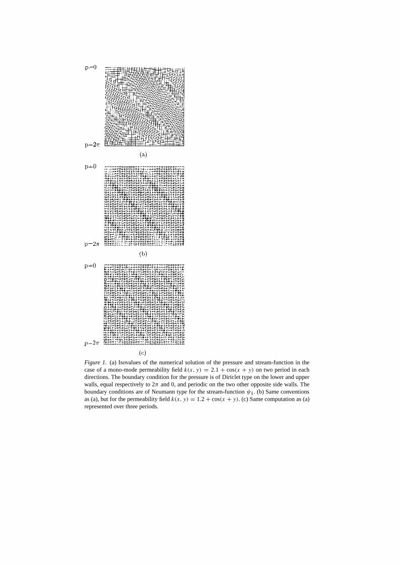
Figure 1. (a) Isovalues of the numerical solution of the pressure and stream-function in thecase of a mono-mode permeability field k(x, y) = 2.1 + cos(x + y) on two period in eachdirections. The boundary condition for the pressure is of Diriclet type on the lower and upperwalls, equal respectively to 2π and 0, and periodic on the two other opposite side walls. Theboundary conditions are of Neumann type for the stream-function ψ1. (b) Same conventionsas (a), but for the permeability field k(x, y) = 1.2 + cos(x + y). (c) Same computation as (a)represented over three periods.

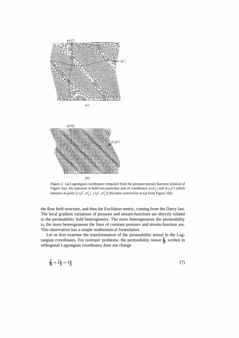
Figure 2. (a) Lagrangian coordinates computed from the pressure/stream-function solution ofFigure 1(a). We represent in bold two particular sets of coordinates p(ψ ′

1) and ψ1(p′) which

intersect at point(x(p′, ψ ′

1), y(p′, ψ ′

1))

(b) same convection as (a) from Figure 1(b).

the flow field structure, and thus the Euclidean metric, coming from the Darcy law.The local gradient variations of pressure and stream-functions are directly relatedto the permeability field heterogeneity. The more heterogeneous the permeabilityis, the more heterogeneous the lines of constant pressure and stream-function are.This observation has a simple mathematical formulation.

Let us first examine the transformation of the permeability tensor in the Lag-rangian coordinates. For isotropic problems, the permeability tensor k, written inorthogonal Lagrangian coordinates does not change

k = kI = kI. (7)

From Darcy’s Equation (1), it follows that in two dimensions we have

k = k = ‖∇ψ1‖‖∇p‖ =

√g22

g11, (8)

and in three dimensions:

k = k = ‖∇ψ2‖ ‖∇ψ3‖‖∇p‖ =

√g22g33

g11. (9)

Thus relation (8) is the Darcy law rewritten in the Lagrangian coordinates illus-trated on Figures 2(a) and 2(b).

In the case of curvilinear orthogonal systems of coordinates, differential operat-ors such as gradient and divergence can still be used without a tensorial representa-tion. In the case of transport processes in which convection prevails, it is interestingto examine the Lagrangian convective operator D/Dt of a transported quantity s:

Ds

Dt= ∂s

∂t+ v · ∇s. (10)

Because this operator is hyperbolic, it is a source of numerical difficulties (Aziz andSettari, 1979). When it is expressed in the Lagrangian coordinates, the convectiontransport operator is much more simple. In two dimensions, it reads

Ds

Dt= ∂s

∂t+ ‖∇p‖ ‖∇ψ1‖ ∂s

∂p, (11)

and in three dimensions:

Ds

Dt= ∂s

∂t+ ‖∇p‖ ‖∇ψ2‖ ‖∇ψ3‖ ∂s

∂p. (12)

We can see that in the two- and three-dimensional cases, this operator is one di-mensional in the Lagrangian coordinates, as expected from the construction of thecoordinates. To illustrate this basic property, we compute the front position of apurely convected tracer in Figure 3 from the integration of the velocity field alongthe stream-lines obtained on Figure 2. The front roughness is directly linked withthe velocity fluctuations, and hence the permeability field heterogeneities.

Let us now express the transport operator (2) in the Lagrangian coordinates. Inthe case of a scalar permeability, it is easy to show that in two dimensions, for anyscalar field s we have

div(k∇s) = √g

(∂2s

∂p2+ ∂

∂ψ1

([‖∇ψ1‖‖∇p‖

]2∂s

∂ψ1

)), (13)

div

(1

k∇s

)= √

g

(∂

∂p

([ ‖∇p‖‖∇ψ1‖

]2∂s

∂p

)+ ∂2s

∂ψ21

), (14)

Figure 3. (a) Convection at infinite Peclet number of a tracer front from an horizontal lineon the below wall through the heterogeneous permeability field of Figure 1(a). The tracerfronts are displayed with bold lines at different equally spaced times, while stream-lines arerepresented with thin line. (b) Same convention as (a) from Figure 1(b).

where g is the determinant of the contravariant metric tensor: g = det gij =‖∇p‖2‖∇ψ1‖2. Note that these transport operators are homogeneous in one dir-ection. This property is called a partial tensorisation of the transport operator (2) inLagrangian coordinates. This property remains for the three-dimensional versionof the first operator (13)

div(k∇s) = √g

(∂2s

∂p2+ ∂

∂ψ2

([‖∇ψ2‖‖∇p‖

]2∂s

∂ψ2

)+ ∂

∂ψ3

([‖∇ψ3‖‖∇p‖

]2∂s

∂ψ3

)),

(15)

where g = detgij = ‖∇p‖2‖∇ψ2‖2‖∇ψ3‖2. However, the three-dimensional ver-

sion of the operator (14) is not homogeneous and reads

div

(1

k∇s

)= √

g

(∂

∂p

([‖∇ψ2‖‖∇ψ3‖‖∇p‖

]2∂s

∂p

)+

+ ∂

∂ψ2

(‖∇ψ3‖2 ∂s

∂ψ2

)+ ∂

∂ψ3

(‖∇ψ2‖2 ∂s

∂ψ3

)). (16)

To our knowledge, results (13)–(16) are not documented in the literature. Althoughbasic, they are however remarkable, because of their potential numerical and theor-etical interest. We discuss in Section 2.2 the use of these properties on the efficiencyof numerical computations.

2.1.2. Anisotropic Heterogeneous Permeability

In a case of anisotropic heterogeneous permeability, the pressure and stream-functionobey the following partial differential equations in two dimensions

div(k−1∇ψ1) = div(k ∇p) = 0. (17)

Similar equations for stream-functions in three dimensions can be found (Zijl,1986). These equations with the proper boundary conditions define a curvilin-ear non-orthogonal system of coordinates. There is nevertheless an orthogonalityproperty between the stream-functions gradient and the flux (sometimes calledk-orthogonality)

∇ψi · k ∇p = 0 for i = 1, 2, 3. (18)

This relation is less simple than in the isotropic case. Figure 4 displays two ex-amples of pressure/stream-function solutions for a fully tensorial permeability field.The gradients of pressure p and stream-function ψ1 are not orthogonal as can beobserved in the computed Lagrangian coordinates of Figure 5. Another importantdifference with the isotropic case concerns the permeability tensor k in the Lag-rangian coordinates which is different from its original expression k. Note first that

its expression can be simplified because k is symmetric: kT = k. Consequently,

the transformed tensor k is symmetric kT = k. Moreover, it is easy to show that k

is diagonal. Let us prove this important property in two dimensions, the extensionto the three-dimensional case being obvious.

The non-diagonal coefficients of the permeability tensor are obtained by usingthe metric tensor of the coordinate change

k12 = ∂p

∂x

∂ψ1

∂xk11 + ∂p

∂y

∂ψ1

∂yk22 + k12

(∂p

∂x

∂ψ1

∂y+ ∂p

∂y

∂ψ1

∂x

). (19)

The right hand side of this relation is exactly identical to relation (18) in twodimensions so that k12 = 0 and k21 = 0. The covariant form of the permeability

Figure 4. Same computation as Figure 1 but in the case of a full tensorial permeability field,k11(x, y) = 2.1 + cos(x + y), k12 = 1 = k21, k22(x, y) = 2.1 + cos(2(x + y)). One canclearly observe the non-orthogonality of the pressure and stream-function.

Figure 5. Lagrangian coordinates computed from Figure 4.

tensor is thus diagonal and reads

k11 =(∂p

∂x

)2

k11 +(∂p

∂y

)2

k22 + 2∂p

∂x

∂p

∂yk12,

k22 =(∂ψ1

∂x

)2

k11 +(∂ψ1

∂y

)2

k22 + 2∂ψ1

∂x

∂ψ1

∂yk12. (20)

This remarkable property holds in the three-dimensional case provided that k issymmetrical. This result was already differently derived in (Edwards et al., 1998)in two dimensions.

Figure 6. Same computation as in Figure 3 for convection at infinite Peclet number in the fulltensorial permeability field of Figure 4 on Lagrangian coordinates computed in Figure 5.

Recall that in the isotropic case, the metric is diagonal. This does not hold inthe anisotropic case where in two dimensions the contravariant form of the metrictensor reads

gij ≡( ∇p2 ∇p · ∇ψ1

∇p · ∇ψ1 ∇ψ21

). (21)

In three dimensions, the stream-function gradients can be chosen orthogonal andthe covariant form of the metric tensor becomes

gij ≡ ∇p2 ∇p · ∇ψ2 ∇p · ∇ψ3

∇p · ∇ψ2 ∇ψ22 0

∇p · ∇ψ3 0 ∇ψ23

. (22)

The Lagrangian coordinate system is defined by two sets of mutually orthogonalvectors (ei) and (ei ): (ei · ej ) = δ

j

i . The contravariant bases are defined by (e1 =∇p, e2 = ∇ψ1) and (e1 = ∇p, e2 = ∇ψ2, e3 = ∇ψ3) in two and three dimen-sions, respectively. As we did when dealing with the isotropic case, we turn to theexpression of the convective transport operator (10) in the Lagrangian coordinates.Using the tensorial notation, it reads

Ds

Dt= ∂s

∂t+ v · (eigij ∂j s) = ∂s

∂t+ v · (ei∂is

). (23)

In two dimensions the velocity is orthogonal to the stream-function gradient: v =e1 (‖e2‖/‖e1‖) so that Equation (23) becomes

Ds

Dt= ∂s

∂t+ ‖∇ψ1‖√

g11

∂s

∂p. (24)

This property has a simple physical interpretation, since, even if isobar lines areno more orthogonal with stream-lines, stream-lines remain the convection traject-ory by definition. This is illustrated in Figure 6 in the case of two fully tensorialpermeability fields.

In three dimensions we have: v = e2 × e3 = e1(‖e2‖‖e3‖/‖e1‖). Equation (23)becomes

Ds

Dt= ∂s

∂t+ ‖∇ψ2‖‖∇ψ3‖√

g11

∂s

∂p. (25)

An important advantage of the coordinate change is that in both the two- andthree-dimensional cases, the convection operator is one dimensional. Moreover thetransport tensorial Equation (13) reads in two dimensions

√g∂l (k

li∂is) = √

g

(∂

∂p

(k11

√g

∂s

∂p

)+ ∂

∂ψ1

(k22

√g

∂s

∂ψ1

)), (26)

where g is the determinant of the contravariant metric tensor: g = detgij. In three

dimensions it becomes

√g∂l (k

li∂is) = √

g

(∂

∂p

(k11

√g

∂s

∂p

)+ ∂

∂ψ2

(k22

√g

∂s

∂ψ2

)+

+ ∂

∂ψ3

(k33

√g

∂s

∂ψ3

)). (27)

Thus kij

acts as an effective diagonal permeability tensor for the heterogeneoustransport equations written in the Lagrangian coordinates. This important prop-erty, may be exploited in the numerical computation of transport with a tensorialpermeability (Edwards et al., 1998) as will be discussed in the next section.

2.2. APPLICATION TO PASSIVE OR ACTIVE TRANSPORT PROCESSES

In the case of passive scalar transport, diffusion and convection play antagonistroles according to the permeability heterogeneity. Convection enhances heterogen-eity by a non-local integration of the velocity field fluctuations, while diffusiontends to erase the specific permeability field structure. When convection prevailsover diffusion, the specific structure of the permeability field can thus influencetransport.

As indicated in the last subsection, the convection operator (10) is one dimen-sional in the Lagrangian coordinates for both isotropic and anisotropic media. Inthe limit of infinite Peclet numbers, this property enables one to compute the disper-sion curves in an efficient and accurate way and a straightforward parallelization ofthe dispersion convective process can be applied. Figure 3(a) shows the tracer frontcomputed from the Lagrangian coordinates of Figure 2(a). In the non-infinite Pecletnumber limit, the coordinate system can be effectively used to solve the hyperbolictransport equation, which is a source of numerical difficulties in heterogeneousmedia (Saad et al., 1990).

Active transport can also be very precisely and effectively computed in the Lag-rangian coordinates (Cirpka and Kitanidis, 2000). Particles deposed or re-convected

depending on the local values of the velocity field are of interest in numerousapplications (Gruesbeck and Collns, 1982; Dowel-Boyer et al., 1986). The typicalsize of these particles is generally large enough to make their diffusion weak so thatthe Peclet number is large. Hence, the particle motion is governed by a convectionequation of type (10) which makes the Lagrangian coordinate projection useful.The local permeability k(x, t) is an autonomous function on the time t and dependson the concentration of particles: k(x, t) ≡ k(x, s(x, t)). Such formulation althoughcommonly used in practical applications — for example in crystallization process(Yeum et al., 1989; Beckermann et al. 1988) or dissolution (Fredd et al., 1998)— is not obvious. The chosen function k(x, s(x, t)) describes phenomenologicallythe complex micro-structural coupling between geometry modification and massflow, particles or solute, at the pore scale. Nevertheless, this modification occurs ata time scale much larger than the typical convection through a pore. In this contextof time decoupling, such formulation can be theoretically justified and some expli-cit computation can be done on particular geometries, for example, in the contextof solidification in mushy zones (Goyeau, 1999). Hence in the quasi-steady-statelimit commonly used (Gruesbeck, 1982; Dowell-Boyer, et al., 1986), the transportEquation (2) is time dependent through the concentration s(t) which depends onthe Darcy flux v. In this situation, we may take advantage of the projection of thetransport equation onto the Lagrangian coordinates in order to solve the problemnumerically.

The numerical procedure implies computing the pressure and the stream func-tion at instant t using k(x, s(x, t)) and then to integrate the transport equation alongthe obtained streamlines to get s(t + %t). The easy computation of the convectivepart of this problem, is not the only advantage of Lagrangian coordinates. The newLagrangian coordinates at instant t + %t has to be found. One straightforwardmethod is to compute the new Lagrangian coordinates by means of an iterativelinear solver, since (p(t +%t),ψ(t +%t)) are close to (p(t), ψ(t)). An alternativemethod consists in using the fact that the operators (13) and (15,16) are tensorizedin the p direction. To be more precise, the operator (2) at instant t + %t can beapproached by using a Taylor expansion of the same operator at the instant t :

div(k(t + %t)∇p(t + %t))

= div(k(t)∇p(t + %t)) + div(δk∇F l[p(t)]) + O(%tl+1)

= √g

(∂2p(t + %t)

∂p(t)2+ ∂

∂ψ1(t)

([‖∇ψ1(t)‖‖∇p(t)‖

]2∂p(t + %t)

∂ψ1

))+

+ div(δk∇F l[p(t)]

) + O(%tl+1), (28)

where δk = k(t+%t)−k(t) and F l[p(t)] is lth order Taylor expansion of p(t+%t).Hence, the pressure and stream-functions coordinates at instant t + %t are solvedon the coordinate system made of the Lagrangian coordinates at instant t . Due tothe fact that the dependence of the pressure p(t+%t) on p(t) is dissociated from itsdependence on ψ(t), the computation of p(t + %t) can be achieved by means of a

partial diagonalization method (Higgins and Leighton, 1962; Haidvogel and Zang,1979) in the p direction. The main interest of this method is that it does not requirethe computation and inversion of a matrix whose size would be Np × Nψ1 in two-dimensions where Np and Nψ1 are the numbers of unknowns in each directions.Such a method should be particularly effective in three dimensions (Higgins andLeighton, 1962).

The same method can be set forth in the case of other complex transports suchas dissolution and re-precipitation (Cussler, 1982). Another interesting applicationof the effective solving scheme (28) is the Theis formulation of the pressure dif-fusion problem. The pressure measurement in well tests is a powerful and populartool in the characterization of well logs permeability field (de Swaan, 1976). Themeasure of the pressure variations δp in time around an imposed pressure referencePref provides information on the effective permeability field. When linearizing thecompressible effects of the fluid filling the porous media, the pressure evolutioncan be described by the following equation:

αPref

∂P

∂t= −div(k∇p), (29)

where αPref = 1/ρ[∂ρφ/∂P ]Pref involves the derivatives of the fluid density ρ andporosity φ product ρφ evaluated at the pressure reference Pref. The transformationof the right hand side of equation (29) in the Lagrangian coordinates operator (13)can thus be applied to the resolution of equation (29) with a efficient partiallydiagonalization method.

In the case of anisotropic media, the transport operators (17) are heterogeneousin all directions. Nevertheless, the transformed permeability tensor is diagonalin the Lagrangian coordinates. A priori this property cannot be used in order toimprove the numerical procedure but can be helpful to overcome numerical diffi-culties encountered in the calculus of pressure field in a full tensorial permeabil-ity field (Yanosik and McCracken, 1979; Durlofsky, 1991; Edwards and Rogers,1994). Tensorial permeability field permits, with finite volume discretization, togain much precision in the numerical calculus. Hence in Lagrangian coordinates,scheme order can be lowered with the same accuracy as the Cartesian resolution(Edwards et al., 1998). This property could prove to be very useful in the numericalcomputation of flows in complex anisotropic reservoirs.

3. Two-Phase Flow

Two-phase flows in porous media averaged over the pore scale are described by thegeneralized Darcy relation

Vj (x) = −K(x)krjµj

(∇Pj (x) − ρjG), with j = 1, 2, (30)

where Pj ,Vj and µj are the pressure, velocity and viscosity of the phase j respect-ively and G is the gravity field. K is the intrinsic porous media permeability tensor,

krj and ρj are relative permeability and density of the phase j . In agreement withMuskat (1948), we have

krj ≡ krj (sj ), (31)

where sj is the saturation of the phase j , with s1 + s2 = 1 and krj are the di-agonal components of the relative permeability tensor. In what follows we willconsider, to simplify the issue, the second phase saturation s2. We will refer toEquations (30) and (31) as the Darcy–Muskat (DM) model for two phase flowsin porous media. Over the last decades, many authors have proposed (and some-times demonstrated) a full tensorial extension of the relative permeability concept(De Gennes, 1983; S. Whitaker, 1986; Kalaydjian and Legait, 1988; Bear andBachmat, 1991; Liang and Lohrentz, 1994; Dullien and Dong, 1996; Lasseux et al.,1996).

In the present section, we first introduce the main hypothesis and the dimension-less variables. Next we examine the diagonal generalized two-phase flow model(30) in which there is no direct coupling between the pressure gradient and the fluxof each phase. Finally we turn to the case of a full tensorial relative permeabilitywhich will prove to be an easy generalization of the diagonal case.

3.1. DIMENSIONLESS VARIABLES

On a geological scale, intrinsic permeability as well as wettability heterogeneitiesof porous rocks on the scale of the elementary representative volume are crucialparameters which influence the macroscopic properties. The coupling between thephase saturation and the pressure difference between the phases is described by thephenomenological capillary pressure curve

P−(x, s2(x)) = P2(x) − P1(x) = Pc(x, s2(x)). (32)

Although this relation is history-dependent, we assume (as is usually done in manyapplications) that the pressure difference between the phases is a single valuedfunction of the saturation. This assumption is correct for a single run along thehysteresis curve such as single drainage or imbibition process. In the context ofreservoir simulations, such approximations are commonly used (Aziz and Settari,1979; Chavent and Jaffre, 1986).

The (DM) model can be formulated in condensed form by means of the globalstream-function (Higgins and Leighton, 1962; Glimm et al., 1983; Blunt et al.,1996). Since the total flux is divergence free for incompressible flows, a globalstream-function can be defined in two dimensions as V+(x) = V1 + V2 = ∇ ×���1+(x). The three dimensional version of this definition is V+ = ∇�2+ × ∇�3+.The global velocity V+, stream-functions �i+ (i = 1, 2, 3), the pressure sumP+ = P1 + P2 and the gravity are non-dimensionalized by 〈‖V+‖〉, 〈�i+〉, 〈P+〉and |G|, respectively. For our purpose, we also define the viscosity mean µ =(µ1 + µ2)/2, the composed densities ρ+ = ρ1 + ρ2 and ρ− = ρ2 − ρ1 and thenon-dimensionalized composed mobilities

kr+ = µ

(kr1

µ1+ kr2

µ2

)and kr− = µ

(kr2

µ2− kr1

µ1

).

Following Leverett (Leverett, 1940; Bear and Bachmat, 1991), we introduce thedimensionless capillary pressure p−(x, s2) = √〈K〉P−(x, s2)/σ where σ is the in-terfacial tension between the phases and 〈K〉 the averaged permeability. We definea capillary number Ca = (µ〈V+〉/σ )(�/

√〈K〉) constructed from the averagedDarcy flux 〈‖V+‖〉, the mean viscosity µ, the ratio between the typical correlationlength of the heterogeneity � and at typical pore size

√〈K〉. This dimensionlessnumber is a measure of the capillary forces on the scale of one elementary repres-entative volume. The Bond number Bo = ρ−G〈K〉2/σ estimates the ratio betweengravity and capillarity forces.

3.2. DARCY–MUSKAT MODEL WITH SCALAR PERMEABILITY k = kI

Relation (30) can be rewritten with the previously defined variables

1

K(x)kr+V+(x) = − 1

2µ

(∇P+(x) + kr−

kr+∇P−(x, s2) −

(ρ+ + ρ−

kr−kr+

)G).

(33)

We define the global pressure ∇P ∗+ (Verruijt and Barends, 1981; Chavent andJaffre, 1986; Plouraboue, 1998) by

∇P ∗+ = 1

2

(∇P+(x) + kr−

kr+(s2)(∇P−(x) − ∇xPc(x, s2)) − ρ+G

), (34)

where

∇P− = ∇xPc + ∂P

∂s2∇s2. (35)

The global pressure P ∗+ has to be defined from relation (34) with a gauge condition.The curl of a vectorial field has to be chosen and can be defined from the boundaryconditions. Equation (33) can be rewritten in a form similar to that of the Darcyequation between the global stream-function and the global pressure. Insertingthe global pressure into Equation (33), the dimensionless version of the resultingequation is

1

k(x)kr+v+ + ∇p∗

+ = − 1

Ca

kr−2kr+

(∇xpc(x, s2) − Bo g) . (36)

The global pressure was first introduced mathematically (Chavent and Jaffre, 1986)to provide a unique variable which takes into account the coupling between thesaturation field and the pressure fields. His definition was rather different from theone given here, integrating relation (34) and choosing a specific boundary conditionto fix the gauge. The Darcy like structure of relation (36) shows that this variable is

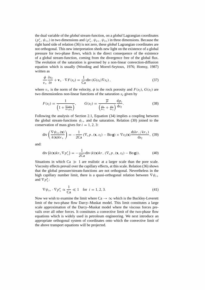
the dual variable of the global stream-function, on a global Lagrangian coordinates(p∗+, ψ1+) in two dimensions and (p∗+, ψ2+, ψ3+) in three dimensions. Because theright hand side of relation (36) is not zero, these global Lagrangian coordinates arenot orthogonal. This new interpretation sheds new light on the existence of a globalpressure for two-phase flows, which is the direct consequence of the existenceof a global stream-function, coming from the divergence free of the global flux.The evolution of the saturation is governed by a non-linear convection-diffusionequation which is usually (Wooding and Morrel-Seytoux, 1976; Homsy, 1987)written as

φ

v+∂s2

∂t+ v+ · ∇F(s2) = 1

Cadiv (G(s2)∇s2) , (37)

where v+ is the norm of the velocity, φ is the rock porosity and F(s2), G(s2) aretwo dimensionless non-linear functions of the saturation s2 given by

F(s2) = 1(1 + kr2µ1

kr1µ2

) , G(s2) = µ(µ1kr1

+ µ2kr2

) dpc

ds2. (38)

Following the analysis of Section 2.1, Equation (34) implies a coupling betweenthe global stream-functions ψi+ and the saturation. Relation (30) joined to theconservation of mass gives for i = 1, 2, 3:

div

(∇ψ1+(x)k(x)kr+

)= − 1

2Ca(∇xp−(x, s2) − Bo g) × ∇s2(x)

d(kr−/kr+)ds2

, (39)

and:

div(k(x)kr+∇p∗

+) = − 1

2Cadiv (k(x)kr− (∇xp−(x, s2) − Bo g)). (40)

Situations in which Ca � 1 are realistic at a larger scale than the pore scale.Viscosity effects prevail over the capillary effects, at this scale. Relation (36) showsthat the global pressure/stream-functions are not orthogonal. Nevertheless in thehigh capillary number limit, there is a quasi-orthogonal relation between ∇ψi+and ∇p�+:

∇ψi+ · ∇p�+ ∝ 1

Ca� 1 for i = 1, 2, 3. (41)

Now we wish to examine the limit where Ca → ∞ which is the Buckley-Leverettlimit of the two-phase flow Darcy–Muskat model. This limit constitutes a largescale approximation of the Darcy–Muskat model where the viscous forces pre-vails over all other forces. It constitutes a convective limit of the two-phase flowequations which is widely used in petroleum engineering. We next introduce anappropriate orthogonal system of coordinates onto which the convective limit ofthe above transport equations will be projected.

3.3. THE BUCKLEY–LEVERETT LIMIT OF THE (DM) EQUATIONS

In such situations, many numerical analyses have used the stream-function co-ordinate to study the Darcy–Muskat model in two dimensions (Garcia et al., 1998;Edwards et al., 1998). Some extensions of these methods have been carried out inisotropic three dimensional permeability fields, without an explicit computation ofthe stream-functions, but using a random walk Lagrangian reconstruction of thestream-lines (Blunt et al., 1996).

In the present section, we show how the formalism presented in Section 2.1 canbe used in the study of two-phase flows in porous media in the Buckley–Leverettlimit. The orthogonal system of coordinates and the formal analogy between theequations make it possible to do so.

We note with a superscript 0 variables which are solutions of the (DM) modelin the limit Ca → ∞. We define the dimensionless variables using the notationsintroduced in the preceding subsection. We thus define the velocity v0+, stream-functions ψ0

i+ with i = 1, 2, 3 and global pressure p�0+ so that equation (36) reads

v0+(x) = −k(x)kr+(s0

2 )∇p�0+ (x), (42)

with v0+ = ∇ × ψ01+ in two dimensions and v0+ = ∇ψ0

2+ × ∇ψ03+ in three dimen-

sions. From Equation (42) and the incompressibility constraint of each phase, wehave

div

(1

kkr+(s02 )

∇ψ01+

)= div

(kkr+(s0

2 )∇P �0+) = 0 for i = 1, 2, 3. (43)

As was previously mentioned, Equation (42) indicates that the global stream func-tions ∇ψ0

i+ and the global pressure ∇p�0+ are orthogonal. In this limit we can definethe associated saturation s0

2 whose evolution is described by a purely convectiveequation

φ

v+∂s0

2

∂t+ v0

+ · ∇F(s02 ) = 0. (44)

As already observed in Section 2.1, in the coordinates (p�0+ , ψ0i+) the non-linear

convective operator is one-dimensional. This simplification is one of the majorreasons for the popularity of streamlines methods (Blunt et al., 1996). Neverthelesseven when one dimensional, the integration of equation (44) requires a specificnumerical treatment with high order numerical schemes (Aziz and Settari, 1979;Douglas and Yrang, 1984; Saad et al., 1990). According to what has been statedin Section 2.1, the transport operator (43) can be rewritten in the Buckley–Leverettcoordinates (p�0+ , ψ0

i+) where it is homogeneous in the p�0+ direction. This propertycan be exploited to simplify the numerical computation of three dimensional prob-lems as mentioned in Section 2.2. In the next subsection, we focus on the influenceof finite capillary numbers.

3.4. GENERAL (DM) MODEL WITH LARGE CAPILLARY NUMBERS

Global Lagrangian coordinates can be extended to the general resolution of Equa-tions (37), (39) and (40) in the presence of capillary forces at large capillary num-bers. The idea of this section is to compute the real global pressure/stream-functionwith an iterative procedure, starting from the zero order of the Buckley–Leverettsolution. Such an iterative scheme can also be used to take into account some gra-vity effects coming from a density difference between phases. We illustrate sucha procedure on the first correction terms to show explicitly the generalization inthe case of non-zero capillarity pressure. We expand the fields in power series ofthe 1/Ca

v+ = v0+ + 1

Cav1

+ + · · · ,

s2 = s02 + 1

Cas1

2 + · · · ,

p�+ = p�0

+ + 1

Cap�1

+ + ··,

ψi+ = ψ0i+ + 1

Caψ1

i+ + · · for i = 1, 2, 3. (45)

From Equation (45) we write the equation for the perturbation of the saturation s12

φ

v+∂s1

2

∂t+ v0

+ · ∇s12F

′′(s0

2 ) = −v1+ · ∇F(s0

2 ) + div(G(s0

2 )∇s02

), (46)

where F ′′ denotes the second derivative of F relative to s2. The left-hand side of Ex-pression (46) is the operator acting on s1

2 . The right-hand side of Equation (46) doesnot depend on s1

2 . Note also that the left-hand side of Equation (46) is one dimen-sional when it is rewritten in the Buckley–Leverett coordinates (p�0+ , ψ0

i+). Hencethe transport Equation (46) of the saturation correction s1

2 can be transformed intoan hyperbolic one-dimensional equation. The same simplification holds for the firstorder perturbation of the pressure which verifies:

div(k(x)kr+(s02)∇p�1

+ ) = −div(k(x)kr−(s02 )(∇xp−(x, s0

2 ) + Bo g))

−div(s12k(x)kr

′+(s

02 )∇p∗0

+ ). (47)

Again, the left-hand side is a transport operator acting on p�1+ and the right-handside does not depend on p�1+ . The transport operator can be rewritten in the(p�0+ , ψ0

i+) coordinates where it becomes homogeneous in the p�0+ direction. Again,this property can be used to increase the efficiency of the computation of the globalpressure correction. The same method can be applied to higher order correctionsof pressure and stream-functions.

3.5. TENSOR PERMEABILITY k AND NON DIAGONAL RELATIVE

PERMEABILITY kr

We are now turning to the case in which the permeability is a tensor, while therelative permeability is a diagonal tensor. Equations (36), (39) and (40) can beeasily extended to a tensorial permeability field k as in Section 2.1

k−1(x)kr−1+ v+ = −∇p∗

+ − 1

2Ca

kr−kr+

(∇xpc(x, s2) + Bo g) , (48)

and for i = 1, 2, 3

div(k−1(x)kr−1

+ ∇ψi+(x))

= − 1

2Ca(∇xp−(x, s2) + Bo g) × ∇s2(x)

d(kr−/kr+)ds2

. (49)

In this case, the global Lagrangian coordinates are not orthogonal even in theBuckley–Leverett limit. Instead, at finite capillary numbers, we find

∇ψi · kkr+∇p�+ ∝ 1

Cafor i = 1, 2, 3, (50)

and in the Buckley–Leverett limit

∇ψ0i · kkr+∇p�0

+ = 0 for i = 1, 2, 3. (51)

As was previously mentioned, the convection operator is one dimensional in theBuckley–Leverett limit even in the case of anisotropic permeability fields whenit is expressed in the Buckley–Leverett Lagrangian coordinates in two on threedimensions. Hence the whole analysis can be used to simplify the numerical com-putation of the time integration of the hyperbolic equation. The Buckley–LeverettLagrangian coordinates are also useful for computing the capillary correction tothe purely viscous case.

The case of tensorial relative permeability can also be of interest at least froma theoretical point of view. It is difficult to assess its practical interest owing to thelack of experimental results concerning the values of the non-diagonal componentsof the relative permeability. However the generalization of the above method canbe applied with minor changes in the definition of kr+ and kr−:

kr+ = µ

(kr1

µ1+ kr2

µ1+ kr12

µ2+ kr21

µ1

),

kr− = µ

(−kr1

µ1+ kr2

µ1− kr12

µ2+ kr21

µ1

), (52)

where kr is defined by

kr ≡(

kr11 kr12

kr21 kr22

). (53)

4. Conclusion

In this paper, we have presented a systematic examination of the properties ofLagrangian coordinates and their potential usefulness for numerical computationin porous media flows. This formulation, which applies, for the most general het-erogeneous porous media in two or three dimensions, has been described in detailin the case of different one-phase flow transport processes, and in the case of thetwo-phase flow Darcy–Muskat model.

For one-phase flows we have discussed the significance of these coordinates foractive transport, which involves a coupling of convection with some complex pro-cesses. We also showed the interest of Lagrangian coordinates for the computationof pressure diffusion problems due to a partial tensorisation of transport operator.In the case of an anisotropic symmetric permeability tensor, we showed that thepermeability tensor is diagonal in the Lagrangian coordinates system.

For two-phase flows, we have extended the results obtained in (Plouraboue,1998) to anisotropic permeability fields and to three dimensions. General globalLagrangian coordinate provide a new interpretation for the existence of a globalpressure for two-phase flows. These coordinates give a rigorous and formal back-ground to ‘stream-line’ methods as well as some new insights into their gener-alization. In the limit of infinite capillary numbers (Buckley–Leverett limit), thegeneralized global Lagrangian coordinates system is orthogonal. The hyperbolicnon-linear convection of the phase saturation is one dimensional along the globalpressure coordinate. At finite capillary numbers or when it exists a density gradientbetween phases, the orthogonality does not hold any more. We have proposed ageneralization of ‘stream-line’ method via an iterative scheme for finite Capil-lary numbers and/or with non-zero Bond number. We illustrated such an iterativeprocedure that takes into account capillary effects.

We hope that these results will provide a new framework for future improve-ments of Lagrangian numerical simulations in porous media flows.

Acknowledgement

The authors thank Dr. F. Belghacem for fruitful discussions.

References

Aziz, K. and Settari, A.: 1979, Petroleum Reservoir Simulation, Applied Science Publisher, London.Bear, J. and Bachmat, Y.: 1991, Introduction to Modeling of Transport Phenomena in Porous Media,

Dover Publications NY, Elsevier Publishing Company.Beckermann, C. and Viskanta, R.: 1998, Phys. Chem. Hydro.Blunt, M. J., Luii, K. and Thiele, M. R.: 1996, A generalized streamline method to predict reservoirs

flows, Petrol. Geosci. 2, 259–269.Bratvedt, F., Gimse, T. and Tegnander, C.: 1996, Streamline computations for porous media flow

including gravity, Transport in Porous Media 25(1), 63–78.

Chavent, G. and Jaffr, J.: 1986, Mathematical Models and Finite Elements for Reservoir Simulation,North-Holland, Amsterdam.

Cirpka, O. A. and Kitanidis, P. K.: 2000, An advective-dispersive stream-tube approach for thetransfer of concervative-tracer data to reactive transport, Water Resour. Res. 36(5), 1209–1220.

Cussler, E. L.: 1982, Dissolution and reprecipitation in porous media, AIChE 128(3), 500.Douglas, J. and Yrang, Y.: 1984, Numerical simulation of immiscible flow in porous media based

on combining the method of characteristics with mixed finite element procedures, IMA 11,122–131.

Mc Dowell-Boyer, L., Hunt, J. R. and Sitar, N.: 1986, Particle transport through porous media, WaterResour. Res. 22(13), 1901–1921.

Dullien, F. A. L. and Dong, M.: 1996, Experimental determination of the flow transport coefficientsin the coupled equations of two-phase flow in porous media, Transport in Porous Media 25,97–120.

Durlofsky, L. J.: 1991, Numerical calculations of equivalent gridblock permeability tensors forheterogeneous porous media, Water Resour. Res. 27(5), 699–708.

Edwards, M. G., Agut, R. and Aziz, K.: 1998, Quasi-orthogonal streamline grids: gridding and anddiscretization, SPE 49072, 1–13, 7–10.

Edwards, M. G. and Rogers, C. F.: 1994, A flux continuous scheme for the full tensor pressureequation. ECMOR IV, Topic D, Simulation of fluid flow: 1–8, 7–10.

Fredd, C. N. and Fogler, H. S.: 1998, Influence of transport and reaction on wormhole formation inporous media, AIChE J. 44(9), 1933–1949.

Garcia, M., Journel, A. G. and Aziz, K.: 1998, An automatic grid generation and adjustement methodfor modeling reservoirs heterogeneities, Soc. Petrol. Eng..

De Gennes, P. G.: 1983, Theory of slow biphasic flow in porous media, Phys. Chem. Hydrol. 4,175–185.

Glimm, J., Isaacson, E., Marchesin, D. and McBryan, O.: 1983, A front tracking reservoir simulator,five spot validation studies and the water coning problem, Math. Res. Sim. 107–136.

Goyeau, B., Benihaddadene, T., Gobin, D. and Quintard, M.: 1999, Numerical calculation of thepermeability in a dendritic mushy zone, Metallurg. Mat. Trans. B 30B, 613–622.

Gruesbeck, C. and Collns, R. E.: 1982, Entrainment and deposition of fine particles in porous media,Soc. Petrol. Ing. 22(6), 847–856.

Haidvogel, D. B. and Zang, T.: 1979, The accurate solution of Poisson’s equation by expansion inchebyshev polynomials, J. Comp. Phys. 30, 167–180.

Hansen, A., Roux, S., Aharony, A., Feder, J., Jossang, T. and Hardy, H. H.: 1997, Real-spacerenormalization estimates for two-phase flow in porous media, Transport in Porous Media 29,247–279.

Higgins, R. V. and Leighton, A. J.: 1962, A computer method to calculate two-phase flow in anyirregular bounded porous medium, J. Petrol. Technol. 14, 679–683.

Homsy, G. M.: 1987, Viscous fingering in porous media. Ann. Rev. Fluid. Mech. 19, 271–311.Kalaydjian, F. and Legait, B.: 1988, J. Phys. II 23(6).Yeum, K.S., Laxmanan, V. and Poirier, D. R.: 1989, Efficient estimation of diffusion during dendritic

solidification, Metall. Trans. A.Lasseux, D., Quintard, M. and Whitaker, S.: 1996, Determination of permeability tensor for two-

phase flow in heterogeneous porous media: theory, Transport in Porous Media 2, 107–137.Leverett, M. C.: 1940, Capillary behavior in porous solid, J. Pet. Tech 2, 1–17.Liang, Q. and Lohrentz, J.: 1994, Transport in Porous Media 15, 71–79.Matanga, G. B.: 1993, Stream-functions in three-dimensional groundwater flows, Water Resour. Res.

29(9), 3125–3133.Mehrabi, A. R. and Sahimi, M.: 1997, Coarsening of heterogeneous media: application of wavelets,

Phys. Rev. Lett. 79(22), 4385–4388.Muskat, M.: 1948, The theory of potentiometric models, Trans AIME 179, 216–221.

Plouraboue, F.: 1998, A new coordinate system for two-phase darcy-muskat flows in heterogeneousisotropic porous media in two dimensions, C. R. Acad. Sci. Paris 2, 326(2).

Saad, N., pope, G. A. and Sepehrnoori, K.: 1990, Application of highter-order methods incompositional simulation, SPE Res. Eng. 623–630.

de Swaan, O. A.: 1976, Analytic solutions for determining naturally fractured reservoirs propertiesby well testing, Trans. AIME.

Whitaker, S.: 1986, The governing equations of immiscible two phase flow, Transport in PorousMedia 1, 105–125.

Verruijt, A. and Barends, F. B. J.: 1981, The global pressure, a new concept for the modelizationof compressible two-phase flow in porous media, in: G. Chavent and Barends (eds), Flow andTransport in Porous Media, Balkeman, Rotterdam.

Wooding, R. A. and Morrel-Seytoux, H. J.: 1976, Multiphase flow through porous media, Ann. Rev.Fluid. Mech. 8(2), 233–274.

Yanosik, J. L. and McCracken, T. A.: 1979, A nine point finite difference recervoir simulator forrealistic prediction of adverse mobility ratio displacements, SPE J. 253–262.

Zijl, W.: 1986, Numerical simulation based on stream function and velocities in three dimensionnalgroundwater flow, J. Hydrol. 85, 349–365.