Generalized inverseFrom Wikipedia, the free encyclopedia

Contents

1 Division (mathematics) 11.1 Notation . . . . . . . . . . . . . . . . . . . . . . . . . . . . . . . . . . . . . . . . . . . . . . . . 11.2 Computing . . . . . . . . . . . . . . . . . . . . . . . . . . . . . . . . . . . . . . . . . . . . . . 3

1.2.1 Manual methods . . . . . . . . . . . . . . . . . . . . . . . . . . . . . . . . . . . . . . . 31.2.2 By computer or with computer assistance . . . . . . . . . . . . . . . . . . . . . . . . . . . 4

1.3 Properties . . . . . . . . . . . . . . . . . . . . . . . . . . . . . . . . . . . . . . . . . . . . . . . 41.4 Euclidean division . . . . . . . . . . . . . . . . . . . . . . . . . . . . . . . . . . . . . . . . . . . 41.5 Of integers . . . . . . . . . . . . . . . . . . . . . . . . . . . . . . . . . . . . . . . . . . . . . . 41.6 Of rational numbers . . . . . . . . . . . . . . . . . . . . . . . . . . . . . . . . . . . . . . . . . . 51.7 Of real numbers . . . . . . . . . . . . . . . . . . . . . . . . . . . . . . . . . . . . . . . . . . . . 51.8 By zero . . . . . . . . . . . . . . . . . . . . . . . . . . . . . . . . . . . . . . . . . . . . . . . . 51.9 Of complex numbers . . . . . . . . . . . . . . . . . . . . . . . . . . . . . . . . . . . . . . . . . 51.10 Of polynomials . . . . . . . . . . . . . . . . . . . . . . . . . . . . . . . . . . . . . . . . . . . . 51.11 Of matrices . . . . . . . . . . . . . . . . . . . . . . . . . . . . . . . . . . . . . . . . . . . . . . 6

1.11.1 Left and right division . . . . . . . . . . . . . . . . . . . . . . . . . . . . . . . . . . . . 61.11.2 Pseudoinverse . . . . . . . . . . . . . . . . . . . . . . . . . . . . . . . . . . . . . . . . 6

1.12 In abstract algebra . . . . . . . . . . . . . . . . . . . . . . . . . . . . . . . . . . . . . . . . . . . 61.13 Calculus . . . . . . . . . . . . . . . . . . . . . . . . . . . . . . . . . . . . . . . . . . . . . . . . 61.14 See also . . . . . . . . . . . . . . . . . . . . . . . . . . . . . . . . . . . . . . . . . . . . . . . . 61.15 References . . . . . . . . . . . . . . . . . . . . . . . . . . . . . . . . . . . . . . . . . . . . . . 71.16 External links . . . . . . . . . . . . . . . . . . . . . . . . . . . . . . . . . . . . . . . . . . . . . 7

2 Generalized inverse 82.1 Types of generalized inverses . . . . . . . . . . . . . . . . . . . . . . . . . . . . . . . . . . . . . 82.2 Uses . . . . . . . . . . . . . . . . . . . . . . . . . . . . . . . . . . . . . . . . . . . . . . . . . . 82.3 See also . . . . . . . . . . . . . . . . . . . . . . . . . . . . . . . . . . . . . . . . . . . . . . . . 92.4 References . . . . . . . . . . . . . . . . . . . . . . . . . . . . . . . . . . . . . . . . . . . . . . 92.5 External links . . . . . . . . . . . . . . . . . . . . . . . . . . . . . . . . . . . . . . . . . . . . . 9

3 Moore–Penrose pseudoinverse 103.1 Notation . . . . . . . . . . . . . . . . . . . . . . . . . . . . . . . . . . . . . . . . . . . . . . . . 103.2 Definition . . . . . . . . . . . . . . . . . . . . . . . . . . . . . . . . . . . . . . . . . . . . . . . 103.3 Properties . . . . . . . . . . . . . . . . . . . . . . . . . . . . . . . . . . . . . . . . . . . . . . . 11

i

ii CONTENTS

3.3.1 Existence and uniqueness . . . . . . . . . . . . . . . . . . . . . . . . . . . . . . . . . . . 113.3.2 Basic properties . . . . . . . . . . . . . . . . . . . . . . . . . . . . . . . . . . . . . . . . 113.3.3 Reduction to Hermitian case . . . . . . . . . . . . . . . . . . . . . . . . . . . . . . . . . 123.3.4 Products . . . . . . . . . . . . . . . . . . . . . . . . . . . . . . . . . . . . . . . . . . . . 123.3.5 Projectors . . . . . . . . . . . . . . . . . . . . . . . . . . . . . . . . . . . . . . . . . . . 123.3.6 Geometric construction . . . . . . . . . . . . . . . . . . . . . . . . . . . . . . . . . . . . 133.3.7 Subspaces . . . . . . . . . . . . . . . . . . . . . . . . . . . . . . . . . . . . . . . . . . . 133.3.8 Limit relations . . . . . . . . . . . . . . . . . . . . . . . . . . . . . . . . . . . . . . . . 133.3.9 Continuity . . . . . . . . . . . . . . . . . . . . . . . . . . . . . . . . . . . . . . . . . . . 133.3.10 Derivative . . . . . . . . . . . . . . . . . . . . . . . . . . . . . . . . . . . . . . . . . . . 13

3.4 Special cases . . . . . . . . . . . . . . . . . . . . . . . . . . . . . . . . . . . . . . . . . . . . . . 133.4.1 Scalars . . . . . . . . . . . . . . . . . . . . . . . . . . . . . . . . . . . . . . . . . . . . 133.4.2 Vectors . . . . . . . . . . . . . . . . . . . . . . . . . . . . . . . . . . . . . . . . . . . . 143.4.3 Linearly independent columns . . . . . . . . . . . . . . . . . . . . . . . . . . . . . . . . 143.4.4 Linearly independent rows . . . . . . . . . . . . . . . . . . . . . . . . . . . . . . . . . . 143.4.5 Orthonormal columns or rows . . . . . . . . . . . . . . . . . . . . . . . . . . . . . . . . 143.4.6 Circulant matrices . . . . . . . . . . . . . . . . . . . . . . . . . . . . . . . . . . . . . . . 14

3.5 Construction . . . . . . . . . . . . . . . . . . . . . . . . . . . . . . . . . . . . . . . . . . . . . . 143.5.1 Rank decomposition . . . . . . . . . . . . . . . . . . . . . . . . . . . . . . . . . . . . . 143.5.2 The QR method . . . . . . . . . . . . . . . . . . . . . . . . . . . . . . . . . . . . . . . . 153.5.3 Singular value decomposition (SVD) . . . . . . . . . . . . . . . . . . . . . . . . . . . . . 153.5.4 Block matrices . . . . . . . . . . . . . . . . . . . . . . . . . . . . . . . . . . . . . . . . 153.5.5 The iterative method of Ben-Israel and Cohen . . . . . . . . . . . . . . . . . . . . . . . . 153.5.6 Updating the pseudoinverse . . . . . . . . . . . . . . . . . . . . . . . . . . . . . . . . . . 163.5.7 Software libraries . . . . . . . . . . . . . . . . . . . . . . . . . . . . . . . . . . . . . . . 16

3.6 Applications . . . . . . . . . . . . . . . . . . . . . . . . . . . . . . . . . . . . . . . . . . . . . . 163.6.1 Linear least-squares . . . . . . . . . . . . . . . . . . . . . . . . . . . . . . . . . . . . . . 163.6.2 Obtaining all solutions of a linear system . . . . . . . . . . . . . . . . . . . . . . . . . . . 163.6.3 Minimum norm solution to a linear system . . . . . . . . . . . . . . . . . . . . . . . . . . 173.6.4 Condition number . . . . . . . . . . . . . . . . . . . . . . . . . . . . . . . . . . . . . . . 17

3.7 Generalizations . . . . . . . . . . . . . . . . . . . . . . . . . . . . . . . . . . . . . . . . . . . . 173.8 See also . . . . . . . . . . . . . . . . . . . . . . . . . . . . . . . . . . . . . . . . . . . . . . . . 173.9 References . . . . . . . . . . . . . . . . . . . . . . . . . . . . . . . . . . . . . . . . . . . . . . . 183.10 External links . . . . . . . . . . . . . . . . . . . . . . . . . . . . . . . . . . . . . . . . . . . . . 193.11 Text and image sources, contributors, and licenses . . . . . . . . . . . . . . . . . . . . . . . . . . 20

3.11.1 Text . . . . . . . . . . . . . . . . . . . . . . . . . . . . . . . . . . . . . . . . . . . . . . 203.11.2 Images . . . . . . . . . . . . . . . . . . . . . . . . . . . . . . . . . . . . . . . . . . . . 203.11.3 Content license . . . . . . . . . . . . . . . . . . . . . . . . . . . . . . . . . . . . . . . . 21

Chapter 1

Division (mathematics)

This article is about the arithmetical operation. For other uses, see Division (disambiguation).“Divided” redirects here. For other uses, see Divided (disambiguation).In mathematics, especially in elementary arithmetic, division (denoted ÷ or / or —) is an arithmetic operation.Specifically, if b times c equals a, written:

a = b × c

where b is not zero, then a divided by b equals c, written:

a ÷ b = c, a/b = c, or ab = c.

For instance,

6 ÷ 3 = 2

since

3 × 2 = 6.

In the above expressions, a is called the dividend, b is called the divisor, and c is called the quotient; in the expressiona/b or a

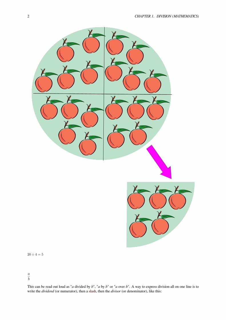
b , a is also called the numerator and b is also called the denominator.Conceptually, division of integers can be viewed in either of two distinct but related ways quotition and partition:

• Partitioning involves taking a set of size a and forming b groups that are equal in size. The size of each groupformed, c, is the quotient of a and b.

• Quotition, or quotative division (also sometimes spelled quotitive) involves taking a set of size a and forminggroups of size b. The number of groups of this size that can be formed, c, is the quotient of a and b.[1] (Bothdivisions give the same result because multiplication is commutative.)

Teaching division usually leads to the concept of fractions being introduced to school pupils. Unlike addition,subtraction, and multiplication, the set of all integers is not closed under division. Dividing two integers may re-sult in a remainder. To complete the division of the remainder, the number system is extended to include fractionsor rational numbers as they are more generally called.

1.1 Notation

Division is often shown in algebra and science by placing the dividend over the divisor with a horizontal line, alsocalled a fraction bar, between them. For example, a divided by b is written

1

2 CHAPTER 1. DIVISION (MATHEMATICS)

20÷ 4 = 5

a

b

This can be read out loud as "a divided by b", "a by b" or "a over b". A way to express division all on one line is towrite the dividend (or numerator), then a slash, then the divisor (or denominator), like this:

1.2. COMPUTING 3

a/b

This is the usual way to specify division in most computer programming languages since it can easily be typed as asimple sequence of ASCII characters. Some mathematical software, such as GNU Octave, allows the operands to bewritten in the reverse order by using the backslash as the division operator:

b\a

A typographical variation halfway between these two forms uses a solidus (fraction slash) but elevates the dividend,and lowers the divisor:

a⁄b

Any of these forms can be used to display a fraction. A fraction is a division expression where both dividend anddivisor are integers (typically called the numerator and denominator), and there is no implication that the divisionmust be evaluated further. A second way to show division is to use the obelus (or division sign), common in arithmetic,in this manner:

a÷ b

This form is infrequent except in elementary arithmetic. ISO 80000-2−9.6 states it should not be used. The obelusis also used alone to represent the division operation itself, as for instance as a label on a key of a calculator.In some non-English-speaking cultures, “a divided by b” is written a : b. This notation was introduced in 1631 byWilliam Oughtred in his Clavis Mathematicae and later popularized by Gottfried Wilhelm Leibniz.[2] However, inEnglish usage the colon is restricted to expressing the related concept of ratios (then "a is to b").In elementary classes of some countries, the notation b) a or b)a is used to denote a divided by b, especially whendiscussing long division; similarly, but less commonly, b)a for short division (as shown in an example on that page).This notation was first introduced by Michael Stifel in Arithmetica integra, published in 1544.[2]

1.2 Computing

Main article: Division algorithm

1.2.1 Manual methods

Division is often introduced through the notion of “sharing out” a set of objects, for example a pile of sweets, into anumber of equal portions. Distributing the objects several at a time in each round of sharing to each portion leads tothe idea of "chunking", i.e., division by repeated subtraction.More systematic andmore efficient (but also more formalised andmore rule-based, andmore removed from an overallholistic picture of what division is achieving), a person who knows the multiplication tables can divide two integersusing pencil and paper using the method of short division, if the divisor is simple. Long division is used for largerinteger divisors. If the dividend has a fractional part (expressed as a decimal fraction), one can continue the algorithmpast the ones place as far as desired. If the divisor has a fractional part, we can restate the problem by moving thedecimal to the right in both numbers until the divisor has no fraction.A person can calculate division with an abacus by repeatedly placing the dividend on the abacus, and then subtractingthe divisor the offset of each digit in the result, counting the number of divisions possible at each offset.A person can use logarithm tables to divide two numbers, by subtracting the two numbers’ logarithms, then lookingup the antilogarithm of the result.A person can calculate division with a slide rule by aligning the divisor on the C scale with the dividend on the Dscale. The quotient can be found on the D scale where it is aligned with the left index on the C scale. The user isresponsible, however, for mentally keeping track of the decimal point.

4 CHAPTER 1. DIVISION (MATHEMATICS)

1.2.2 By computer or with computer assistance

Modern computers compute division by methods that are faster than long division: see Division algorithm.In modular arithmetic, some numbers have a multiplicative inverse with respect to the modulus. We can calculatedivision by multiplication in such a case. This approach is useful in computers that do not have a fast divisioninstruction.

1.3 Properties

Division is right-distributive over addition and subtraction. That means:

a+ b

c= (a+ b)÷ c =

a

c+

b

c

in the same way as in multiplication (a+ b)× c = a× c+ b× c . But division is not left-distributive, i.e. we have

a

b+ c= a÷ (b+ c) ̸= a

b+

a

c

unlike multiplication.

1.4 Euclidean division

Main article: Euclidean division

The Euclidean division is the mathematical formulation of the outcome of the usual process of division of integers.It asserts that, given two integers, a, the dividend, and b, the divisor, such that b ≠ 0, there are unique integers q, thequotient, and r, the remainder, such that a = bq + r and 0 ≤ r < | b |, where | b | denotes the absolute value of b.

1.5 Of integers

Division of integers is not closed. Apart from division by zero being undefined, the quotient is not an integer unlessthe dividend is an integer multiple of the divisor. For example, 26 cannot be divided by 11 to give an integer. Sucha case uses one of five approaches:

1. Say that 26 cannot be divided by 11; division becomes a partial function.

2. Give an approximate answer as a decimal fraction or a mixed number, so 2611 ≃ 2.36 or 26

11 ≃ 2 36100 . This is the

approach usually taken in numerical computation.

3. Give the answer as a fraction representing a rational number, so the result of the division of 26 by 11 is 2611 .

But, usually, the resulting fraction should be simplified: the result of the division of 52 by 22 is also 2611 . This

simplification may be done by factoring out the greatest common divisor.

4. Give the answer as an integer quotient and a remainder, so 2611 = 2 remainder 4. To make the distinction with

the previous case, this division, with two integers as result, is sometimes called Euclidean division, because itis the basis of the Euclidean algorithm.

5. Give the integer quotient as the answer, so 2611 = 2. This is sometimes called integer division.

Dividing integers in a computer program requires special care. Some programming languages, such as C, treat integerdivision as in case 5 above, so the answer is an integer. Other languages, such asMATLAB and every computer algebrasystem return a rational number as the answer, as in case 3 above. These languages also provide functions to get theresults of the other cases, either directly or from the result of case 3.

1.6. OF RATIONAL NUMBERS 5

Names and symbols used for integer division include div, /, \, and %. Definitions vary regarding integer division whenthe dividend or the divisor is negative: rounding may be toward zero (so called T-division) or toward −∞ (F-division);rarer styles can occur – see Modulo operation for the details.Divisibility rules can sometimes be used to quickly determine whether one integer divides exactly into another.

1.6 Of rational numbers

The result of dividing two rational numbers is another rational number when the divisor is not 0. The division of tworational numbers p/q and r/s is defined as

p/q

r/s=

p

q× s

r=

ps

qr.

All four quantities are integers, and only p may be 0. This definition ensures that division is the inverse operation ofmultiplication.

1.7 Of real numbers

Division of two real numbers results in another real number when the divisor is not 0. It is defined such a/b = c if andonly if a = cb and b ≠ 0.

1.8 By zero

Main article: Division by zero

Division of any number by zero (where the divisor is zero) is undefined. This is because zero multiplied by any finitenumber always results in a product of zero. Entry of such an expression into most calculators produces an errormessage.

1.9 Of complex numbers

Dividing two complex numbers results in another complex number when the divisor is not 0, which is defined as:

p+ iq

r + is=

(p+ iq)(r − is)

(r + is)(r − is)=

pr + qs+ i(qr − ps)

r2 + s2=

pr + qs

r2 + s2+ i

qr − ps

r2 + s2.

All four quantities p, q, r, s are real numbers, and r and s may not both be 0.Division for complex numbers expressed in polar form is simpler than the definition above:

peiq

reis=

peiqe−is

reise−is=

p

rei(q−s).

Again all four quantities p, q, r, s are real numbers, and r may not be 0.

1.10 Of polynomials

One can define the division operation for polynomials in one variable over a field. Then, as in the case of integers,one has a remainder. See Euclidean division of polynomials, and, for hand-written computation, polynomial longdivision or synthetic division.

6 CHAPTER 1. DIVISION (MATHEMATICS)

1.11 Of matrices

One can define a division operation for matrices. The usual way to do this is to define A / B = AB−1, where B−1 denotesthe inverse of B, but it is far more common to write out AB−1 explicitly to avoid confusion.

1.11.1 Left and right division

Because matrix multiplication is not commutative, one can also define a left division or so-called backslash-divisionas A \ B = A−1B. For this to be well defined, B−1 need not exist, however A−1 does need to exist. To avoid confusion,division as defined by A / B = AB−1 is sometimes called right division or slash-division in this context.Note that with left and right division defined this way, A/(BC) is in general not the same as (A/B)/C and nor is (AB)\Cthe same as A\(B\C), but A/(BC) = (A/C)/B and (AB)\C = B\(A\C).

1.11.2 Pseudoinverse

To avoid problemswhenA−1 and/orB−1 do not exist, division can also be defined asmultiplicationwith the pseudoinverse,i.e., A / B = AB+ and A \ B = A+B, where A+ and B+ denote the pseudoinverse of A and B.

1.12 In abstract algebra

In abstract algebras such as matrix algebras and quaternion algebras, fractions such as ab are typically defined as

a · 1b or a · b−1 where b is presumed an invertible element (i.e., there exists a multiplicative inverse b−1 such that

bb−1 = b−1b = 1 where 1 is the multiplicative identity). In an integral domain where such elements may not exist,division can still be performed on equations of the form ab = ac or ba = ca by left or right cancellation, respectively.More generally “division” in the sense of “cancellation” can be done in any ring with the aforementioned cancellationproperties. If such a ring is finite, then by an application of the pigeonhole principle, every nonzero element of thering is invertible, so division by any nonzero element is possible in such a ring. To learn about when algebras (in thetechnical sense) have a division operation, refer to the page on division algebras. In particular Bott periodicity canbe used to show that any real normed division algebra must be isomorphic to either the real numbers R, the complexnumbers C, the quaternions H, or the octonions O.

1.13 Calculus

The derivative of the quotient of two functions is given by the quotient rule:

(f

g

)′

=f ′g − fg′

g2.

1.14 See also• 400AD Sunzi division algorithm

• Division by two

• Field

• Fraction (mathematics)

• Galley division

• Group

• Inverse element

1.15. REFERENCES 7

• Order of operations

• Quasigroup (left division)

• Repeating decimal

1.15 References[1] Fosnot and Dolk 2001. Young Mathematicians at Work: Constructing Multiplication and Division. Portsmouth, NH: Heine-

mann.

[2] Earliest Uses of Symbols of Operation, Jeff MIller

1.16 External links• Division at PlanetMath.org.

• Division on a Japanese abacus selected from Abacus: Mystery of the Bead

• Chinese Short Division Techniques on a Suan Pan

• Rules of divisibility

Chapter 2

Generalized inverse

“Pseudoinverse” redirects here. For the Moore–Penrose pseudoinverse, sometimes referred to as “the pseudoin-verse”, see Moore–Penrose pseudoinverse.

In mathematics, a generalized inverse of a matrix A is a matrix that has some properties of the inverse matrix of Abut not necessarily all of them. Formally, given a matrix A ∈ Rn×m and a matrix Ag ∈ Rm×n , Ag is a generalizedinverse of A if it satisfies the condition AAgA = A .The purpose of constructing a generalized inverse is to obtain a matrix that can serve as the inverse in some sensefor a wider class of matrices than invertible ones. A generalized inverse exists for an arbitrary matrix, and when amatrix has an inverse, then this inverse is its unique generalized inverse. Some generalized inverses can be defined inany mathematical structure that involves associative multiplication, that is, in a semigroup.

2.1 Types of generalized inverses

The Penrose conditions are used to define different generalized inverses: for A ∈ Rn×m and Ag ∈ Rm×n,

If Ag satisfies condition (1.), it is a generalized inverse of A , if it satisfies conditions (1.) and (2.) then it is ageneralized reflexive inverse ofA , and if it satisfies all 4 conditions, then it is a Moore–Penrose pseudoinverse ofA .Other various kinds of generalized inverses include

• One-sided inverse (left inverse or right inverse) If the matrix A has dimensions n×m and is full rank then usethe left inverse if n > m and the right inverse if n < m

• Left inverse is given byA−1left =

(ATA

)−1AT , i.e. A−1

leftA = Im where Im is them×m identity matrix.

• Right inverse is given byA−1right = AT (AAT)−1 , i.e. AA−1

right = In where In is the n×n identity matrix.

• Drazin inverse

• Bott–Duffin inverse

• Moore–Penrose pseudoinverse

2.2 Uses

Any generalized inverse can be used to determine if a system of linear equations has any solutions, and if so to giveall of them.[1] If any solutions exist for the n × m linear system

Ax = b

8

2.3. SEE ALSO 9

with vector x of unknowns and vector b of constants, all solutions are given by

x = Agb+ [I −AgA]w

parametric on the arbitrary vector w, where Ag is any generalized inverse of A. Solutions exist if and only if Agb isa solution – that is, if and only if AAgb = b.

2.3 See also• Inverse element

2.4 References[1] James, M. (June 1978). “The generalised inverse”. Mathematical Gazette 62: 109–114. doi:10.2307/3617665.

• Yoshihiko Nakamura (1991). * Advanced Robotics: Redundancy and Optimization. Addison-Wesley. ISBN0201151987.

• Zheng, B; Bapat, R. B. (2004). “Generalized inverse A(2)T,S and a rank equation”. Applied Mathematics andComputation 155: 407–415. doi:10.1016/S0096-3003(03)00786-0.

• S. L. Campbell and C. D. Meyer (1991). Generalized Inverses of Linear Transformations. Dover. ISBN978-0-486-66693-8.

• Adi Ben-Israel and Thomas N.E. Greville (2003). Generalized inverses. Theory and applications (2nd ed.).New York, NY: Springer. ISBN 0-387-00293-6.

• C. R. Rao and C. Radhakrishna Rao and Sujit Kumar Mitra (1971). Generalized Inverse of Matrices and itsApplications. New York: John Wiley & Sons. p. 240. ISBN 0-471-70821-6.

2.5 External links• 15A09 Matrix inversion, generalized inverses in Mathematics Subject Classification, MathSciNet search

Chapter 3

Moore–Penrose pseudoinverse

In mathematics, and in particular linear algebra, a pseudoinverse A+ of a matrix A is a generalization of the inversematrix.[1] The most widely known type of matrix pseudoinverse is theMoore–Penrose pseudoinverse, which wasindependently described by E. H. Moore[2] in 1920, Arne Bjerhammar[3] in 1951 and Roger Penrose[4] in 1955.Earlier, Fredholm had introduced the concept of a pseudoinverse of integral operators in 1903. When referring toa matrix, the term pseudoinverse, without further specification, is often used to indicate the Moore–Penrose pseu-doinverse. The term generalized inverse is sometimes used as a synonym for pseudoinverse.A common use of the Moore–Penrose pseudoinverse (hereafter, just pseudoinverse) is to compute a 'best fit' (leastsquares) solution to a system of linear equations that lacks a unique solution (see below under §Applications). Anotheruse is to find the minimum (Euclidean) norm solution to a system of linear equations with multiple solutions. Thepseudoinverse facilitates the statement and proof of results in linear algebra.The pseudoinverse is defined and unique for all matrices whose entries are real or complex numbers. It can becomputed using the singular value decomposition.

3.1 Notation

In the following discussion, the following conventions are adopted.

• K will denote one of the fields of real or complex numbers, denoted R, C , respectively. The vector space ofm× n matrices overK is denoted by M(m,n;K) .

• For A ∈ M(m,n;K) , AT and A∗ denote the transpose and Hermitian transpose (also called conjugate trans-pose) respectively. IfK = R , then A∗ = AT .

• For A ∈ M(m,n;K) , then im(A) denotes the range (image) of A (the space spanned by the column vectorsof A ) and ker(A) denotes the kernel (null space) of A .

• Finally, for any positive integer n , In ∈ M(n, n;K) denotes the n× n identity matrix.

3.2 Definition

For A ∈ M(m,n;K) , a pseudoinverse of A is defined as a matrix A+ ∈ M(n,m;K) satisfying all of the followingfour criteria:[4][5]

1. AA+A = A (AA+ need not be the general identity matrix, but it maps all column vectors of A to themselves);

2. A+AA+ = A+ (A+ is a weak inverse for the multiplicative semigroup);

3. (AA+)∗ = AA+ (AA+ is Hermitian); and

4. (A+A)∗ = A+A (A+A is also Hermitian).

10

3.3. PROPERTIES 11

A+ exists for any matrix, A , but when the latter has full rank, A+ can be expressed as a simple algebraic formula.In particular, when A has linearly independent columns (and thus matrix A∗A is invertible), A+ can be computedas:

A+ = (A∗A)−1A∗ .

This particular pseudoinverse constitutes a left inverse, since, in this case, A+A = I .When A has linearly independent rows (matrix AA∗ is invertible), A+ can be computed as:

A+ = A∗(AA∗)−1 .

This is a right inverse, as AA+ = I .

3.3 Properties

Proofs for some of these facts may be found on a separate page here.

3.3.1 Existence and uniqueness

• The pseudoinverse exists and is unique: for any matrix A , there is precisely one matrix A+ , that satisfies thefour properties of the definition.[5]

Amatrix satisfying the first condition of the definition is known as a generalized inverse. If the matrix also satisfies thesecond definition, it is called a generalized reflexive inverse. Generalized inverses always exist but are not in generalunique. Uniqueness is a consequence of the last two conditions.

3.3.2 Basic properties

• If A has real entries, then so does A+ .

• If A is invertible, its pseudoinverse is its inverse. That is: A+ = A−1 .[6]:243

• The pseudoinverse of a zero matrix is its transpose.

• The pseudoinverse of the pseudoinverse is the original matrix: (A+)+ = A .[6]:245

• Pseudoinversion commutes with transposition, conjugation, and taking the conjugate transpose:[6]:245

(AT)+ = (A+)T, (A )+ = A+, (A∗)+ = (A+)∗.

• The pseudoinverse of a scalar multiple of A is the reciprocal multiple of A+:

(αA)+ = α−1A+ for α ̸= 0.

Identities

The following identities can be used to cancel certain subexpressions or expand expressions involving pseudoinverses.Proofs for these properties can be found in the proofs subpage.

12 CHAPTER 3. MOORE–PENROSE PSEUDOINVERSE

A+ = A+ A+∗ A∗

A+ = A∗ A+∗ A+

A = A+∗ A∗ AA = A A∗ A+∗

A∗ = A∗ A A+

A∗ = A+ A A∗

3.3.3 Reduction to Hermitian case

The computation of the pseudoinverse is reducible to its construction in the Hermitian case. This is possible throughthe equivalences:

• A+ = (A∗A)+A∗

• A+ = A∗(AA∗)+

as A∗A and AA∗ are obviously Hermitian.

3.3.4 Products

If A ∈ M(m,n;K), B ∈ M(n, p;K) and either,

• A has orthonormal columns (i.e., A∗A = In ) or,

• B has orthonormal rows (i.e., BB∗ = In ) or,

• A has all columns linearly independent (full column rank) and B has all rows linearly independent (full rowrank) or,

• B = A∗ (i.e., B is the conjugate transpose of A ),

then

(AB)+ ≡ B+A+

The last property yields the equivalences:

(AA∗)+ ≡ A+∗A+

(A∗A)+ ≡ A+A+∗

3.3.5 Projectors

P = AA+ and Q = A+A are orthogonal projection operators – that is, they are Hermitian ( P = P ∗ , Q = Q∗ )and idempotent ( P 2 = P and Q2 = Q ). The following hold:

• PA = A = AQ and A+P = A+ = QA+

• P is the orthogonal projector onto the range of A (which equals the orthogonal complement of the kernel ofA∗ ).

• Q is the orthogonal projector onto the range of A∗ (which equals the orthogonal complement of the kernel ofA ).

• (I − P ) is the orthogonal projector onto the kernel of A∗ .

• (I −Q) is the orthogonal projector onto the kernel of A .[5]

3.4. SPECIAL CASES 13

3.3.6 Geometric construction

If we view the matrix as a linear map A : Kn → Km over a field K then A+ : Km → Kn can be decomposedas follows. We write ⊕ for the direct sum, ⊥ for the orthogonal complement, ker for the kernel of a map, and ranfor the image of a map. Notice that Kn = (kerA)⊥ ⊕ kerA and Km = ranA ⊕ (ranA)⊥ . The restrictionA : (kerA)⊥ → ranA is then an isomorphism. These imply that A+ is defined on ranA to be the inverse of thisisomorphism, and on (ranA)⊥ to be zero.In other words: To findA+b for given b in Km, first project b orthogonally onto the range of A, finding a point p(b) inthe range. Then form A−1({p(b)}), i.e. find those vectors in Kn that A sends to p(b). This will be an affine subspaceof Kn parallel to the kernel of A. The element of this subspace that has the smallest length (i.e. is closest to the origin)is the answer A+b we are looking for. It can be found by taking an arbitrary member of A−1({p(b)}) and projectingit orthogonally onto the orthogonal complement of the kernel of A.This description is closely related to the Minimum norm solution to a linear system.

3.3.7 Subspaces

ker(A+) = ker(A∗)

im(A+) = im(A∗)

3.3.8 Limit relations

• The pseudoinverse are limits:

A+ = limδ↘0(A∗A+ δI)−1A∗ = limδ↘0 A

∗(AA∗ + δI)−1

(see Tikhonov regularization). These limits exist even if (AA∗)−1 or (A∗A)−1 do not exist.[5]:263

3.3.9 Continuity

• In contrast to ordinary matrix inversion, the process of taking pseudoinverses is not continuous: if the sequence(An) converges to the matrix A (in the maximum norm or Frobenius norm, say), then (An)+ need not convergeto A+. However, if all the matrices have the same rank, (An)+ will converge to A+.[7]

3.3.10 Derivative

The derivative of a real valued pseudoinverse matrix which has constant rank at a point xmay be calculated in termsof the derivative of the original matrix:[8]

ddxA

+(x) = −A+

( ddxA

)A+ + A+A+T

( ddxA

T)(

I −AA+)

+(I −A+A

)( ddxA

T)A+TA+

3.4 Special cases

3.4.1 Scalars

It is also possible to define a pseudoinverse for scalars and vectors. This amounts to treating these as matrices. Thepseudoinverse of a scalar x is zero if x is zero and the reciprocal of x otherwise:

x+ =

{0, if x = 0;

x−1, otherwise.

14 CHAPTER 3. MOORE–PENROSE PSEUDOINVERSE

3.4.2 Vectors

The pseudoinverse of the null (all zero) vector is the transposed null vector. The pseudoinverse of a non-null vectoris the conjugate transposed vector divided by its squared magnitude:

x+ =

{0T, if x = 0;x∗

x∗x , otherwise.

3.4.3 Linearly independent columns

If the columns of A are linearly independent (so that m ≥ n ), then A∗A is invertible. In this case, an explicitformula is:[1]

A+ = (A∗A)−1A∗

It follows that A+ is then a left inverse of A : A+A = In .

3.4.4 Linearly independent rows

If the rows of A are linearly independent (so thatm ≤ n ), then AA∗ is invertible. In this case, an explicit formulais:

A+ = A∗(AA∗)−1

It follows that A+ is a right inverse of A : AA+ = Im .

3.4.5 Orthonormal columns or rows

This is a special case of either full column rank or full row rank (treated above). If A has orthonormal columns (A∗A = In ) or orthonormal rows ( AA∗ = Im ), then A+ = A∗ .

3.4.6 Circulant matrices

For a circulant matrix C , the singular value decomposition is given by the Fourier transform, that is the singularvalues are the Fourier coefficients. Let F be the Discrete Fourier Transform (DFT) matrix, then[9]

C = F · Σ · F∗

C+ = F · Σ+ · F∗

3.5 Construction

3.5.1 Rank decomposition

Let r ≤ min(m,n) denote the rank of A ∈ M(m,n;K) . Then A can be (rank) decomposed as A = BC whereB ∈ M(m, r;K) and C ∈ M(r, n;K) are of rank r . Then A+ = C+B+ = C∗(CC∗)−1(B∗B)−1B∗ .

3.5. CONSTRUCTION 15

3.5.2 The QR method

ForK = R orK = C computing the productAA∗ orA∗A and their inverses explicitly is often a source of numericalrounding errors and computational cost in practice. An alternative approach using the QR decomposition of A maybe used instead.Considering the case when A is of full column rank, so that A+ = (A∗A)−1A∗ . Then the Cholesky decompositionA∗A = R∗R , where R is an upper triangular matrix, may be used. Multiplication by the inverse is then done easilyby solving a system with multiple right-hand sides,

A+ = (A∗A)−1A∗ ⇔ (A∗A)A+ = A∗ ⇔ R∗RA+ = A∗

which may be solved by forward substitution followed by back substitution.The Cholesky decomposition may be computed without forming A∗A explicitly, by alternatively using the QR de-composition of A = QR , where Q has orthonormal columns, Q∗Q = I , and R is upper triangular. Then

A∗A = (QR)∗(QR) = R∗Q∗QR = R∗R

so R is the Cholesky factor of A∗A .The case of full row rank is treated similarly by using the formula A+ = A∗(AA∗)−1 and using a similar argument,swapping the roles of A and A∗ .

3.5.3 Singular value decomposition (SVD)

A computationally simple and accurate way to compute the pseudo inverse is by using the singular value decompo-sition.[1][5][10] If A = UΣV ∗ is the singular value decomposition of A, then A+ = V Σ+U∗ . For a rectangulardiagonal matrix such asΣ , we get the pseudo inverse by taking the reciprocal of each non-zero element on the diago-nal, leaving the zeros in place, and then transposing the matrix. In numerical computation, only elements larger thansome small tolerance are taken to be nonzero, and the others are replaced by zeros. For example, in the MATLAB,GNU Octave, or NumPy function pinv, the tolerance is taken to be t = ε⋅max(m,n)⋅max(Σ), where ε is the machineepsilon.The computational cost of this method is dominated by the cost of computing the SVD, which is several times higherthan matrix–matrix multiplication, even if a state-of-the art implementation (such as that of LAPACK) is used.The above procedure shows why taking the pseudo inverse is not a continuous operation: if the original matrix A hasa singular value 0 (a diagonal entry of the matrix Σ above), then modifying A slightly may turn this zero into a tinypositive number, thereby affecting the pseudo inverse dramatically as we now have to take the reciprocal of a tinynumber.

3.5.4 Block matrices

Optimized approaches exist for calculating the pseudoinverse of block structured matrices.

3.5.5 The iterative method of Ben-Israel and Cohen

Another method for computing the pseudoinverse uses the recursion

Ai+1 = 2Ai −AiAAi,

which is sometimes referred to as hyper-power sequence. This recursion produces a sequence converging quadrat-ically to the pseudoinverse of A if it is started with an appropriate A0 satisfying A0A = (A0A)

∗ . The choiceA0 = αA∗ (where 0 < α < 2/σ2

1(A) , with σ1(A) denoting the largest singular value of A ) [11] has been arguednot to be competitive to the method using the SVD mentioned above, because even for moderately ill-conditioned

16 CHAPTER 3. MOORE–PENROSE PSEUDOINVERSE

matrices it takes a long time before Ai enters the region of quadratic convergence.[12] However, if started with A0

already close to the Moore–Penrose pseudoinverse and A0A = (A0A)∗ , for example A0 := (A∗A + δI)−1A∗ ,

convergence is fast (quadratic).

3.5.6 Updating the pseudoinverse

For the cases where A has full row or column rank, and the inverse of the correlation matrix (AA∗ for Awith full rowrank or A∗A for full column rank) is already known, the pseudoinverse for matrices related to A can be computedby applying the Sherman–Morrison–Woodbury formula to update the inverse of the correlation matrix, which mayneed less work. In particular, if the related matrix differs from the original one by only a changed, added or deletedrow or column, incremental algorithms[13][14] exist that exploit the relationship.Similarly, it is possible to update the Cholesky factor when a row or column is added, without creating the inverseof the correlation matrix explicitly. However, updating the pseudoinverse in the general rank-deficient case is muchmore complicated.[15][16]

3.5.7 Software libraries

The package NumPy provides a pseudoinverse calculation through its functions matrix.I and linalg.pinv; its pinvuses the SVD-based algorithm. SciPy adds a function scipy.linalg.pinv that uses a least-squares solver. High qualityimplementations of SVD, QR, and back substitution are available in standard libraries, such as LAPACK. Writingone’s own implementation of SVD is a major programming project that requires a significant numerical expertise. Inspecial circumstances, such as parallel computing or embedded computing, however, alternative implementations byQR or even the use of an explicit inverse might be preferable, and custom implementations may be unavoidable.

3.6 Applications

3.6.1 Linear least-squares

See also: Linear least squares (mathematics)

The pseudoinverse provides a least squares solution to a system of linear equations.[17] For A ∈ M(m,n;K) , givena system of linear equations

Ax = b,

in general, a vector x that solves the systemmay not exist, or if one does exist, it may not be unique. The pseudoinversesolves the “least-squares” problem as follows:

• ∀x ∈ Kn , we have ∥Ax − b∥2 ≥ ∥Az − b∥2 where z = A+b and ∥ · ∥2 denotes the Euclidean norm.This weak inequality holds with equality if and only if x = A+b + (I − A+A)w for any vector w; thisprovides an infinitude of minimizing solutions unless A has full column rank, in which case (I − A+A) is azero matrix.[18]The solution with minimum Euclidean norm is z. [18]

This result is easily extended to systems with multiple right-hand sides, when the Euclidean norm is replaced by theFrobenius norm. Let B ∈ M(m, p;K) .

• ∀X ∈ M(n, p;K) , we have ∥AX −B∥F ≥ ∥AZ −B∥F where Z = A+B and ∥ · ∥F denotes the Frobeniusnorm.

3.6.2 Obtaining all solutions of a linear system

If the linear system

3.7. GENERALIZATIONS 17

Ax = b

has any solutions, they are all given by[19]

x = A+b+ [I −A+A]w

for arbitrary vector w. Solution(s) exist if and only if AA+b = b .[19] If the latter holds, then the solution is uniqueif and only if A has full column rank, in which case [I − A+A] is a zero matrix. If solutions exist but A does nothave full column rank, then we have an indeterminate system, all of whose infinitude of solutions are given by thislast equation. This solution is deeply connected to the Udwadia–Kalaba equation of classical mechanics to forces ofconstraint that do not obey D'Alembert’s principle.

3.6.3 Minimum norm solution to a linear system

For linear systems Ax = b, with non-unique solutions (such as under-determined systems), the pseudoinverse maybe used to construct the solution of minimum Euclidean norm ∥x∥2 among all solutions.

• If Ax = b is satisfiable, the vector z = A+b is a solution, and satisfies ∥z∥2 ≤ ∥x∥2 for all solutions.

This result is easily extended to systems with multiple right-hand sides, when the Euclidean norm is replaced by theFrobenius norm. Let B ∈ M(m, p;K) .

• If AX = B is satisfiable, the matrix Z = A+B is a solution, and satisfies ∥Z∥F ≤ ∥X∥F for all solutions.

3.6.4 Condition number

Using the pseudoinverse and a matrix norm, one can define a condition number for any matrix:

cond(A) = ∥A∥∥A+∥.

A large condition number implies that the problem of finding least-squares solutions to the corresponding system oflinear equations is ill-conditioned in the sense that small errors in the entries of A can lead to huge errors in the entriesof the solution.[20]

3.7 Generalizations

In order to solve more general least-squares problems, one can define Moore–Penrose pseudoinverses for all contin-uous linear operators A : H1 → H2 between two Hilbert spaces H1 and H2, using the same four conditions as in ourdefinition above. It turns out that not every continuous linear operator has a continuous linear pseudoinverse in thissense.[20] Those that do are precisely the ones whose range is closed in H2.In abstract algebra, aMoore–Penrose pseudoinverse may be defined on a *-regular semigroup. This abstract definitioncoincides with the one in linear algebra.

3.8 See also• Proofs involving the Moore–Penrose pseudoinverse

• Drazin inverse

• Hat matrix

18 CHAPTER 3. MOORE–PENROSE PSEUDOINVERSE

• Inverse element

• Linear least squares (mathematics)

• Pseudo-determinant

• Von Neumann regular ring

3.9 References

[1] Ben-Israel, Adi; Thomas N.E. Greville (2003). Generalized Inverses. Springer-Verlag. ISBN 0-387-00293-6.

[2] Moore, E. H. (1920). “On the reciprocal of the general algebraic matrix”. Bulletin of the American Mathematical Society26 (9): 394–395. doi:10.1090/S0002-9904-1920-03322-7.

[3] Bjerhammar, Arne (1951). “Application of calculus of matrices to method of least squares; with special references togeodetic calculations”. Trans. Roy. Inst. Tech. Stockholm 49.

[4] Penrose, Roger (1955). “A generalized inverse for matrices”. Proceedings of the Cambridge Philosophical Society 51:406–413. doi:10.1017/S0305004100030401.

[5] Golub, Gene H.; Charles F. Van Loan (1996). Matrix computations (3rd ed.). Baltimore: Johns Hopkins. pp. 257–258.ISBN 0-8018-5414-8.

[6] Stoer, Josef; Bulirsch, Roland (2002). Introduction to Numerical Analysis (3rd ed.). Berlin, New York: Springer-Verlag.ISBN 978-0-387-95452-3..

[7] Rakočević, Vladimir (1997). “On continuity of the Moore–Penrose and Drazin inverses” (PDF). Matematički Vesnik 49:163–172.

[8] http://www.jstor.org/stable/2156365

[9] Stallings, W. T.; Boullion, T. L. (1972). “The Pseudoinverse of an r-Circulant Matrix”. Proceedings of the AmericanMathematical Society 34: 385–388. doi:10.2307/2038377.

[10] Linear Systems & Pseudo-Inverse

[11] Ben-Israel, Adi; Cohen, Dan (1966). “On Iterative Computation of Generalized Inverses and Associated Projections”.SIAM Journal on Numerical Analysis 3: 410–419. doi:10.1137/0703035. JSTOR 2949637.pdf

[12] Söderström, Torsten; Stewart, G. W. (1974). “On the Numerical Properties of an Iterative Method for Computing theMoore–Penrose Generalized Inverse”. SIAM Journal on Numerical Analysis 11: 61–74. doi:10.1137/0711008. JSTOR2156431.

[13] Tino Gramß (1992). “Worterkennung mit einem künstlichen neuronalen Netzwerk”. Georg-August-Universität zu Göttin-gen.

[14] , Mohammad Emtiyaz, “Updating Inverse of a Matrix When a Column is Added/Removed”

[15] Meyer, Carl D., Jr. Generalized inverses and ranks of block matrices. SIAM J. Appl. Math. 25 (1973), 597–602

[16] Meyer, Carl D., Jr. Generalized inversion of modified matrices. SIAM J. Appl. Math. 24 (1973), 315–323

[17] Penrose, Roger (1956). “On best approximate solution of linear matrix equations”. Proceedings of the Cambridge Philo-sophical Society 52: 17–19. doi:10.1017/S0305004100030929.

[18] Planitz, M., “Inconsistent systems of linear equations”, Mathematical Gazette 63, October 1979, 181–185.

[19] James, M., “The generalised inverse”, Mathematical Gazette 62, June 1978, 109–114.

[20] Roland Hagen, Steffen Roch, Bernd Silbermann. C*-algebras and Numerical Analysis, CRC Press, 2001. Section 2.1.2.

3.10. EXTERNAL LINKS 19

3.10 External links• Pseudoinverse on PlanetMath

• Interactive program & tutorial of Moore–Penrose Pseudoinverse

• Moore–Penrose inverse at PlanetMath.org.

• Weisstein, Eric W., “Pseudoinverse”, MathWorld.

• Weisstein, Eric W., “Moore–Penrose Inverse”, MathWorld.

• The Moore–Penrose Pseudoinverse. A Tutorial Review of the Theory

• Online Moore-Penrose Inverse calculator

20 CHAPTER 3. MOORE–PENROSE PSEUDOINVERSE

3.11 Text and image sources, contributors, and licenses

3.11.1 Text• Division (mathematics) Source: https://en.wikipedia.org/wiki/Division_(mathematics)?oldid=685711520Contributors: AxelBoldt, Mav,Bryan Derksen, The Anome, Hajhouse, Christian List, Toby Bartels, Ortolan88, Mjb, Heron, Patrick, Michael Hardy, Eric119, Ahoer-stemeier, Andres, Emperorbma, Charles Matthews, Dcoetzee, Jitse Niesen, Furrykef, Hyacinth, Saltine, .mau., Jusjih, Robbot, Choco-lateboy, ZimZalaBim, Gandalf61, Henrygb, SvavarL, Moink, Wikibot, Ruakh, Lzur, Tobias Bergemann, ManuelGR, Giftlite, Herbee,Nayuki, CryptoDerk, LiDaobing, Antandrus, Beland, Gauss, Flex, Kate, Gazpacho, PhotoBox, Paul August, Andrejj, Jnestorius, Gauge,MBisanz, Stesmo, Longhair, Robotje, R. S. Shaw, Helopticor, Nk, Zaraki~enwiki, Jumbuck, Frodet, Alansohn, Gary, Keenan Pepper,BaF, Olegalexandrov, Wtmitchell, Jheald, Oleg Alexandrov, Nuno Tavares, Linas, TigerShark, LOL, Ae-a, Chad1m, Gisling, Sukolsak,Jshadias, Josh Parris, Coemgenus, Salix alba, HappyCamper, MarnetteD, Chobot, YurikBot, Wavelength, Hairy Dude, Jengelh, Spuri-ousQ, Wimt, Welsh, Apokryltaros, Brian Crawford, Muu-karhu, Bota47, Brisvegas, Arthur Rubin, MathsIsFun, Kosza, Netch, Smack-Bot, Haymaker, KnowledgeOfSelf, Melchoir, GraemeMcRae, Skizzik, Oli Filth, PrimeHunter, MalafayaBot, Coffin, Octahedron80,MaxSem, Georg-Johann, VMS Mosaic, Jpape, SundarBot, UU, DaniLoveSky, BIL, Mwtoews, Vina-iwbot~enwiki, SashatoBot, Butko,Bjankuloski06en~enwiki, IronGargoyle, Frokor, Mets501, JMK, Quantum7, CRGreathouse, Mudd1, Cydebot, Chuck Marean, Knight-Move, Omicronpersei8, Thijs!bot, Epbr123, Oerjan, Dfrg.msc, Mentifisto, JEBrown87544, .alyn.post., JAnDbot, Hroðulf, VoABot II,Acertain, Ryeterrell, Animum, David Eppstein, Martynas Patasius, Gwern, MartinBot, Arjun01, J.delanoy, Numbo3, Laurusnobilis,SparsityProblem, TomasBat, Joshua Issac, Juliancolton, RJASE1, Idioma-bot, R00723r0, Hellno2, VolkovBot, Am Fiosaigear~enwiki,Philip Trueman, TXiKiBoT, Nono le petit robot~enwiki, Anonymous Dissident, Slysplace, Onore Baka Sama, Houtlijm~enwiki, Jesin,Falcon8765, Chaffers, AlleborgoBot, Symane, SieBot, ToePeu.bot, Paolo.dL, OKBot, Stephen Shaw, Silvergoat, Nn123645, Wahrmund,Into The Fray, Atif.t2, ClueBot, Justin W Smith, Jan1nad, Wysprgr2005, UKoch, Blanchardb, Hardcore Hak, H.Marxen, ProfOak,Thingg, Carltonengesia, Plasmic Physics, Iranway, Addbot, Some jerk on the Internet, Jncraton, Leszek Jańczuk, Mrchapel0203, Tassede-the, Numbo3-bot, VASANTH S.N., Tide rolls, PV=nRT, Legobot, Luckas-bot, Yobot, 2D, Ptbotgourou, Mauler90, Mathtchr, ,AnomieBOT, Erel Segal, Jim1138, IRP, Galt57, Benhen1997, MauritsBot, Xqbot, TinucherianBot II, XZeroBot, Sakaa, Mlpearc, Ishe-den, GrouchoBot, FrescoBot, LucienBOT, Rotideypoc41352, Michael93555, Jmealy718, Majopius, WikiMichel, MacMed, Ramesh-ngbot, EliseVanLooij, Jschnur, Petitvie, Beao, TobeBot, Skakkle, Suffusion of Yellow, DARTH SIDIOUS 2, DASHBot, EmausBot,WikitanvirBot, GoingBatty, Wham Bam Rock II, Tommy2010, AvicBot, Alpha Quadrant (alt), Quondum, D.Lazard, Paulmiko, Chuis-pastonBot, ,28botשדדשכ, Xanchester, ClueBot NG, Aspen1995, Wcherowi, CocuBot, Spel-Punc-Gram, Stapler9124, Helpful Pixie Bot,Calabe1992, John Cummings, Wiki13, ElphiBot, Thumani Mabwe, Hillcrest98, Chmarkine, Glacialfox, The1337gamer, Dysrhythmia,Bombaysippin, William.stoner, Max Buskirk, Manjit2012, Frosty, Mmitchell10, Samsher joon, M.f.ashraf, SuryawanshiAkash, Loraof,Thallior, Manunited 26, KnowAndGrow, KasparBot, Idkmankind123, Trymankind, Snowweatyh and Anonymous: 250

• Generalized inverse Source: https://en.wikipedia.org/wiki/Generalized_inverse?oldid=679140746 Contributors: Kku, Aenar, Pavon,RainerBlome, TedPavlic, Billlion, Oleg Alexandrov, Roboto de Ajvol, Gareth Jones, Zvika, Saippuakauppias, Vanisaac, DivideByZero14,R'n'B, JohnBlackburne, A4bot, Jmath666, Melcombe, DragonBot, PixelBot, Estirabot, Rhuso, GDibyendu, AnomieBOT, Obersachsebot,Tponweiser, RjwilmsiBot, Quondum, AManWithNoPlan, Zfeinst, Helpful Pixie Bot, JohnMathTeacher, Qetuth, DG-on-WP, Monkbot,Astrozot and Anonymous: 13

• Moore–Penrose pseudoinverse Source: https://en.wikipedia.org/wiki/Moore%E2%80%93Penrose_pseudoinverse?oldid=684708505Contributors: AxelBoldt, Michael Hardy, Charles Matthews, Dcoetzee, Jitse Niesen, MH~enwiki, Fredrik, Kaol, Giftlite, BenFrantz-Dale, TomViza, MarkSweep, Simoneau, Sam Hocevar, RainerBlome, Rich Farmbrough, Bender235, Gauge, Billlion, Oyz, 3mta3,Forderud, Galaxiaad, Jfr26, Jeff3000, BD2412, Qwertyus, Rjwilmsi, Salix alba, Mathbot, Yeteez, Gaius Cornelius, Yahya Abdal-Aziz,Entropeneur, Oakwood, Jasón, Teply, Zvika, Lunch, SmackBot, RDBury, InverseHypercube, Ddcampayo, Tgdwyer, Charlesb, Blue-bot, Nbarth, Rludlow, Belizefan, Kaarebrandt, Dan Gluck, A. Pichler, AbsolutDan, Lavaka, CBM, Eric Le Bigot, HenningThiele-mann, Raamin, OrenBochman, JAnDbot, Dirkjot~enwiki, Alexandre Vassalotti, Ensign beedrill, Catskineater, Mathemaduenn~enwiki,K.menin, Shiznick, Squids and Chips, LokiClock, MusicScience, Jmath666, Peeter.joot, D420182, Paolo.dL, Khvalamde, Abelian, Jdg-ilbey, D1ma5ad, Addbot, DOI bot, Yobot, Pcap, Calle, AnomieBOT, SlothMcCarty, Citation bot, Xqbot, Duoduoduo, EmausBot, Johnof Reading, Thecheesykid, Sgoder, Quondum, JordiGH, Zfeinst, Run54, Dschult, Statmolox, Timflutre, CitationCleanerBot, A*-search,ChrisGualtieri, ClausenM, SoledadKabocha, Xdever, DG-on-WP, Monkbot, Leegrc, Loraof, Ruminaik and Anonymous: 92

3.11.2 Images• File:Aspect-ratio-4x3.svg Source: https://upload.wikimedia.org/wikipedia/commons/d/de/Aspect-ratio-4x3.svg License: Public do-main Contributors: own work, manual SVG coding Original artist: Tanya sanderson

• File:Commons-logo.svg Source: https://upload.wikimedia.org/wikipedia/en/4/4a/Commons-logo.svg License: ? Contributors: ? Origi-nal artist: ?

• File:Divide20by4.svg Source: https://upload.wikimedia.org/wikipedia/commons/2/2e/Divide20by4.svg License: Public domain Con-tributors: Own work Original artist: Amirki

• File:Percent_18e.svg Source: https://upload.wikimedia.org/wikipedia/commons/f/f9/Percent_18e.svg License: Public domain Contrib-utors: Created with the DejaVu Sans font and Inkscape. Original artist: Farmer Jan and bdesham

• File:Question_book-new.svg Source: https://upload.wikimedia.org/wikipedia/en/9/99/Question_book-new.svg License: Cc-by-sa-3.0Contributors:Created from scratch in Adobe Illustrator. Based on Image:Question book.png created by User:Equazcion Original artist:Tkgd2007

• File:Rubik’{}s_cube_v3.svg Source: https://upload.wikimedia.org/wikipedia/commons/b/b6/Rubik%27s_cube_v3.svg License: CC-BY-SA-3.0 Contributors: Image:Rubik’{}s cube v2.svg Original artist: User:Booyabazooka, User:Meph666 modified by User:Niabot

• File:Symbol_divide_vote.svg Source: https://upload.wikimedia.org/wikipedia/commons/a/aa/Symbol_divide_vote.svg License: Publicdomain Contributors: ? Original artist: ?

3.11. TEXT AND IMAGE SOURCES, CONTRIBUTORS, AND LICENSES 21

• File:Symbol_multiplication_vote.svg Source: https://upload.wikimedia.org/wikipedia/commons/5/5e/Symbol_multiplication_vote.svgLicense: Public domain Contributors: File:Symbol support2 vote.svg Original artist: TomasBat, Rogilbert, Zscout370

• File:Symbol_oppose_vote.svg Source: https://upload.wikimedia.org/wikipedia/commons/7/7f/Symbol_oppose_vote.svg License: Pub-lic domain Contributors: ? Original artist: ?

• File:Symbol_support_vote.svg Source: https://upload.wikimedia.org/wikipedia/en/9/94/Symbol_support_vote.svg License: Public do-main Contributors: ? Original artist: ?

3.11.3 Content license• Creative Commons Attribution-Share Alike 3.0