1

Generalized Coprime Sampling of Toeplitz Matricesfor Spectrum Estimation

Si Qin, Yimin D. Zhang∗, Senior Member, IEEE, Moeness G. Amin, Fellow, IEEE,and Abdelhak M. Zoubir, Fellow, IEEE

Abstract—Increased demand on spectrum sensing over a broadfrequency band requires a high sampling rate and thus leadsto a prohibitive volume of data samples. In some applications,e.g., spectrum estimation, only the second-order statistics arerequired. In this case, we may use a reduced data sampling rateby exploiting a low-dimensional representation of the originalhigh dimensional signals. In particular, the covariance matrixcan be reconstructed from compressed data by utilizing itsspecific structure, e.g., the Toeplitz property. Among a numberof techniques for compressive covariance sampler design, thecoprime sampler is considered attractive because it enables asystematic design capability with a significantly reduced samplingrate. In this paper, we propose a general coprime samplingscheme that implements effective compression of Toeplitz co-variance matrices. Given a fixed number of data samples, weexamine different schemes on covariance matrix acquisition forperformance evaluation, comparison and optimal design, basedon segmented data sequences.

Index Terms—Compressive covariance sampling, structuredmatrix, coprime sampling, overlapping data segmentation

I. INTRODUCTION

Various applications require spectrum sensing over a broadfrequency band, which demand on the sampling rate and pro-duce a large amount of data. In some cases, the original signalis known to be sparse. This property allows the exploitationof compressive sensing and sparse sampling approaches thatenable effective sparse signal reconstruction [3], [4], with noloss of information. The signal reconstruction can be carriedout by a number of algorithms, such as orthogonal matchingpursuit (OMP), least absolute shrinkage and selection operator(LASSO), and Bayesian compressive sensing [5]–[8].

Spectrum estimation based on the second-order statisticsadds to the abovementioned applications for signal reconstruc-tion. In this case, the covariance function and the covariancematrix can be constructed as low-dimensional representations

Copyright (c) 2016 IEEE. Personal use of this material is permitted.However, permission to use this material for any other purposes must beobtained from the IEEE by sending a request to pubs-permissions@ieee.org.

The work of S. Qin, Y. D. Zhang, and M. G. Amin was supported in partby the Office of Naval Research under Grant No. N00014-13-1-0061. Part ofthe results was presented at the SPIE Mobile Multimedia/Image Processing,Security, and Applications Conference, Baltimore, MD, May 2015 [1], and theIEEE International Conference on Acoustics, Speech, and Signal Processing(ICASSP), Shanghai, China, March 2016 [2].

S. Qin and M. G. Amin are with the Center for Advanced Communications,Villanova University, Villanova, PA 19085, USA.

Y. D. Zhang is with the Department of Electrical and Computer Engineer-ing, Temple University, Philadelphia, PA, 19122, USA.

A. Zoubir is with Signal Processing Group, Technische Universitat Darm-stadt, Darmstadt, Germany.

The corresponding author’s email address is ydzhang@temple.edu.

of the original high-dimensional signals [9], [10]. This fact hasmotivated the development of an alternate framework, referredto as compressive covariance sampling, in which the signalsparsity is not a requirement [11]–[13].

In this paper, we consider spectrum estimation of wide-sense stationary (WSS) processes utilizing the Toeplitz prop-erty of the covariance matrix. Note that, while our focus inthis paper is limited to the second-order statistics, extensionto techniques based on high-order statistics [14] is straightfor-ward.

Several methods have been developed to tackle similar com-pressive Toeplitz matrix sampling. For example, a generalizednested sampler [15] was proposed to recover Toeplitz matricesfrom a compressed covariance matrix. However, this approachassumes an infinite number of data samples and does notconsider the achievable reconstruction performance when thenumber of samples is finite. In addition, it imposes a minimumsampling interval that follows the Nyquist criterion, whichmakes it ineffective to implement low sampling rate systemsfor wideband spectrum estimation. In [16], a minimal sparsesampler was proposed through a set of properly designedanalog filters and then down-sampling the signals at a reducedrate. A finite number of outputs was divided into multipleblocks without overlapping, and the compressed covariancewas estimated by averaging over these blocks. However, therequirement of using the designed analog filters complicatesthe implementation. In addition, the effect of utilization ofoverlapping blocks were not considered.

The proposed work is based on the recently developedcoprime sampling structure [17], which utilizes only twouniform samplers to sample a WSS process with samplingintervals, M and N . The integers M and N , which representthe down-sampling rates, are chosen to be coprime. As aresult, it generates two sets of uniformly spaced samples witha rate substantially lower than the nested [18] and with fewersamplers than the schemes in [19]–[21].

In this paper, we design a sampling matrix to compressToeplitz matrices based on a coprime sampling scheme. Inparticular, our focus is on effective estimations of the Toeplitzcovariance matrix and signal spectrum from a finite numberof samples of a WSS sequence. Toward this objective, wegeneralize the coprime sampling approach to achieve a highernumber of degrees of freedom (DOFs) and low estimationerror. The generalization is carried out in the following twoaspects: (a) The first generalization is to use multiple coprimeunits to obtain a higher number of DOFs and improvedpower spectrum density (PSD) estimation performance. This

2

is achieved through the use of an integer factor p, where acoprime unit is defined as a full period of the output samplepattern between x[bMN ] and x[(b + 1)MN − 1] for anynon-negative integer b. (b) The second generalization is toexploit overlapping blocks in performing sample averaging,enabling an increased number of blocks to be used for sampleaveraging, leading to a reduced estimation variance.

The concept of generalized coprime sampling was firstdeveloped in [1] where only the abovementioned first gen-eralization is considered, whereas the second generation wasintroduced in [2]. In this paper, we extend these preliminaryresults by providing comprehensive theoretical support andperformance bound analysis of the developed techniques,and describe the spectrum estimation algorithm based on thecross-covariance between the outputs of the two samplers. Anumber of simulation results are presented to clearly revealthe relationship between the achieved performance and vari-ous parameters related to the sampling strategies and signalconditions.

The rest of the paper is organized as follows. We firstintroduce the signal model in Section II. Generalized coprimesampling that exploits multiple coprime units is presented inSection III. Section IV describes spectrum estimation based onthe generalized coprime sampling scheme, and the correspond-ing spectrum identifiability, compression factor, and Cramer-Rao bound (CRB) are examined. In Section V, we proposethe exploitation of overlapping samples, and show analyticallythat the overlapping sampling scheme achieves reduced vari-ance in the estimated covariance matrix and signal spectrum.Simulation results are provided in Section VI to numericallyverify the effectiveness of the proposed generalization and theanalysis. Section VII concludes the paper.

Notations: We use lower-case (upper-case) bold charactersto denote vectors (matrices). In particular, IN denotes theN × N identity matrix. (·)∗ implies complex conjugation,whereas (·)T and (·)H respectively denote the transpose andconjugate transpose of a matrix or a vector. E(·) is thestatistical expectation operator and ⊗ denotes the Kroneckerproduct. R and C denote the set of real values and complexvalues, respectively, while N+ denotes the set of positiveintegers. x ∼ CN (a, b) denotes that random variable x followsthe complex Gaussian distribution with mean a and variance b.b·c denotes the floor function which returns the largest integernot exceeding the argument. diag(x) denotes a diagonal matrixthat uses the elements of x as its diagonal elements, andTr{A} returns the trace of matrix A.

II. SIGNAL MODEL

Assume that a zero-mean WSS process X(t), t ∈ R,which consists of signals corresponding to a number ofsparse frequencies, is confined within a bandwidth Bs. Toobtain its PSD, the covariance matrix needs to be providedfrom a specific realization of X(t), t = 0, . . . , T − 1. Itsuffices to consider the discrete-time random process, X[l],obtained by sampling the analog signal X(t), with a Nyquistsampling rate fs = 2Bs. Note that the discrete-time processX[l] remains WSS in the discrete-time sense. Let xL[l] =

[x[l], x[l + 1], . . . , x[l + L− 1]]T be a realized vector of X[l].

Then, the resulting semi-positive definite, Hermitian andToeplitz covariance matrix can be given by

Rx = E[xL[l]xHL [l]

]

=

r[0] r[−1] . . . r[−L+ 1]r[1] r[0] . . . r[−L+ 2]

...... . . .

...r[L− 2] r[L− 3] . . . r[−1]r[L− 1] r[L− 2] . . . r[0]

, (1)

in which the entry r[τ ] = E [x[l]x∗[l − τ ]] only depends on thelags τ = −L+ 1, . . . , L− 1. It is clear from (1) that r[−τ ] =r∗[τ ]. In addition, the Toeplitz structure of Rx implies thatmany of its elements are redundant. As a result, Rx can beobtained from a sparsely sampled data sequence. This factmotivated compressive covariance sampling [11]–[13].

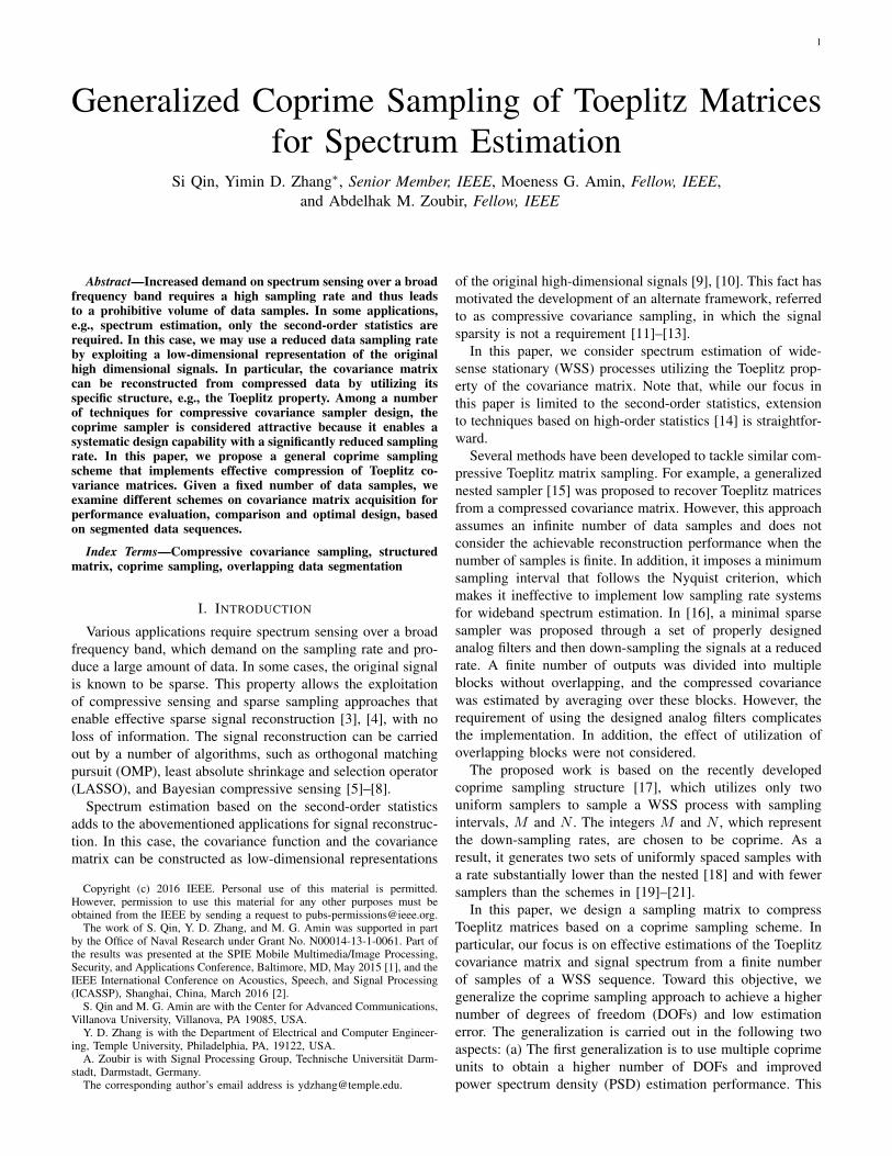
In this paper, we consider the problem of estimating anL × L covariance matrix of xL[l] and the signal PSD froman observation of X(t) with an available length of KTs,where K ∈ N+ and K ≥ L. When sampled at the Nyquistinterval Ts = 1/fs, it yields K samples of discrete-timeobservations x[k], k = 0, . . . ,K − 1. A common practice forcovariance matrix estimation is to segment the entire discrete-time observation of length K into multiple length-L blocks,and average the respectively sample covariances [22]. Asshown in Fig. 1, the entire observation period is segmented intomultiple, possibly overlapping, blocks. In Section III-B, wefirst consider the non-overlapping segmentation to illustrate thesignal model, as shown in Fig. 1(a), whereas the overlappingcase depicted in Fig. 1(b) will be discussed in Section III-C.Denote B as the number of data blocks for the non-overlappingcase. We assume for convenience that the B blocks cover theentire sequence, i.e., BL = K.

Denote by xb[l] = x[l + (b − 1)L], l = 0, . . . , L − 1, andxb = [xb[0], . . . , xb[L − 1]]T for b = 1, . . . , B. We sparselysample each data block using a V ×L sampling matrix As toobtain yb = Asxb, where V � L. The estimated covariancematrix obtained by averaging the available B blocks and isexpressed as

Ry =1

B

B∑b=1

ybyHb = As

(1

B

B∑b=1

xbxHb

)AHs = AsRxAH

s ,

(2)where Rx is an estimated covariance matrix of Rx. Thecompressed covariance matrix Ry with size V × V can beexploited to reconstruct the L × L matrix Rx, provided thatit includes all lags τ = 0, . . . , L − 1. Note that covariancescorresponding to negative lags τ = −L + 1, . . . ,−1 can beobtained through the Hermitian operation r[τ ] = r∗[−τ ] andthus does not contain additional information. Reconstructionof full covariance matrix Rx from the compressed covariancematrix Ry can be made possible by designing a propersampling matrix As. It is clear that, since there are V 2

entries in Ry, the number of samples required to enablereconstruction of the Hermitian Toeplitz matrix Rx is O(

√L).

3

In this end, Rx can be reconstructed as

Rx =

r[0] r[−1] . . . r[−L+ 1]r[1] r[0] . . . r[−L+ 2]

...... . . .

...r[L− 2] r[L− 3] . . . r[−1]r[L− 1] r[L− 2] . . . r[0]

, (3)

where r[τ ], τ = −L+1, . . . , L−1 are estimated by averagingall the entries with the same lag τ in Ry.

0 𝐾 − 1

0 𝐿 − 1

𝐿 2𝐿 − 1

𝐵 − 1 𝐿 𝐾 − 1

𝑥[𝑘]

𝑥1[𝑙]

𝑥2[𝑙]

𝑥𝐵[𝑙]

(a)

0 𝐾 − 1

0 𝐿 − 1

𝐷 𝐷 + 𝐿 − 1

𝐵 − 1 𝐷 𝐾 − 1

𝑥[𝑘]

𝑥1[𝑙]

𝑥2[𝑙]

𝑥𝐵 [𝑙]

(b)

Fig. 1. Illustration of segmentations. (a) Non-overlapping segmentation; (b)Overlapping segmentation.

III. GENERALIZED COPRIME SAMPLING

Coprime sampling exploits two uniform sub-Nyquist sam-plers with sampling period being coprime multiples of theNyquist sampling period [17], [23]. In this section, the general-ized coprime sampling scheme is presented in two operations.A multiple coprime unit factor p ∈ N+ [1], aiming to increasethe number of lags in the compressed covariance matrix, isfirst introduced. Then, the utilization of overlapping samplesbetween blocks is pursued to yield a reduced estimationvariance through the use of a non-overlapping factor q ∈ N+.

A. The concept of coprime sampling

In coprime sampling, the sampling matrix As can bedenoted as As = [AT

s1 ATs2]T , where As1 and As2 are

the sub-sampling matrices corresponding to the two coprimesamplers.

Definition 1: The (i, j)th entry of the sampling matrices As1

and As2 can be designed as:

[As1]i,j =

{1, j = Mi, i ∈ N+,

0, elsewhere,

and

[As2]i,j =

{1, j = Ni, i ∈ N+,

0, elsewhere,(4)

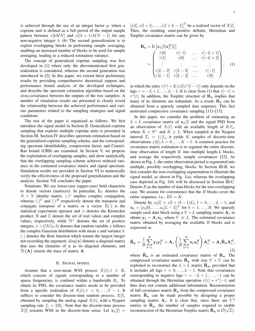
where M ∈ N+ and N ∈ N+ are coprime integers.From a data acquisition perspective, there are two sets of

uniformly spaced samples of the input WSS signal X(t), t =0, . . . , T , from two samplers with sampling intervals MTs andNTs, respectively, as illustrated in Fig. 2. Without loss ofgenerality, we assume M < N . Then, the highest samplingrate of the system is 1/(MTs) = fs/M and the two sampledstream outputs can be given as

y1[k1] = x[Mk1] = X(Mk1Ts),

y2[k2] = x[Nk2] = X(Nk2Ts). (5)

𝑋(𝑡)

𝑁𝑇𝑠

𝑀𝑇𝑠 𝑦1[𝑘1]

𝑦2[𝑘2]

Fig. 2. Coprime sampling structure.

Note that, due to the coprime property of M and N , thereare no overlapping outputs between the two sets other thanx[bMN ] for any non-negative integer b. The outputs betweenx[(b− 1)MN ] and x[bMN − 1] are referred to as a coprimeunit, positioned at

Pb = {bMN +Mk1}⋃{bMN +Nk2}. (6)

Over an observation with an available length of KTs,K/MN coprime units can be obtained, each consists ofM+N physical samples. As such, the total number of physicalsamples is given by

Ks = K

(M +N

MN

)= K

(1

M+

1

N

). (7)

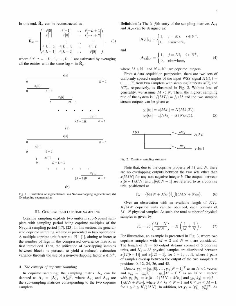
For illustration, an example is presented in Fig. 3, where twocoprime samplers with M = 3 and N = 4 are considered.The length of K = 60 output streams consist of 5 coprimeunits, and Ks = 35 physical samples are distributed betweenx[12(b − 1)] and x[12b − 1], for b = 1, . . . , 5, where 5 pairsof samples overlap between the output of the two samplers atpositions 0, 12, 24, 36, and 48.

Denote yb1 = [yb1 [0], . . . , yb1 [N −1]]T as an N ×1 vector,and yb2 = [yb2 [0], . . . , yb2 [M − 1]]T as an M × 1 vector,with yb1 [k1] = x[(b − 1)MN + Mk1] and yb2 [k2] = x[(b −1)MN +Nk2], where 0 ≤ k1 ≤ N − 1 and 0 ≤ k2 ≤M − 1,for 1 ≤ b ≤ K/(MN). In addition, let yb = [yTb1 yTb2 ]T . As

4

0 3 6 9 12 15 18 21 24 27 30 33 36 39 42 45 48 51 54 57

0 4 8 12 16 20 24 28 32 36 40 44 48 52 56Unit Unit Unit Unit Unit

Fig. 3. An example for coprime sampling (M = 3, and N = 4; •: Nyquistsampler; 4: first sampler outputs; ∇: second sampler outputs.)

such, the (M +N)× (M +N) covariance matrix Ry can beexpressed as

Ry =

Ry11 Ry12

Ry21Ry22

=

E[yb1yHb1

] E[yb1yHb2

]

E[yb2yHb1

] E[yb2yHb2

]

. (8)

In Ry, matrices Ry11 and Ry22 contains self-lags of the twosampler output streams, while their cross-lags are included inmatrices Ry12

and Ry21. Note that Ry21

= R∗y12. In addition,

because the two sampler outputs share the first sample in eachcoprime unit, the self-lags can be taken as cross-lags betweenevery sample from one sampler and the first sample from theother sampler. As such, the self-lags form a subset of thecross-lags. Thus, Rx can be reconstructed by using only Ry12

,whose cross-lags (including the negated ones) are given by thefollowing set,

L = {τ |τ = ±(Mk1 −Nk2)}, (9)

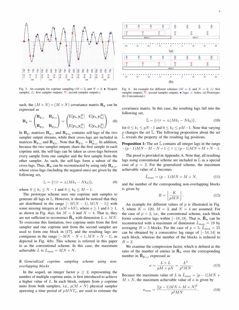
where 0 ≤ k1 ≤ N − 1 and 0 ≤ k2 ≤M − 1.The prototype scheme uses one coprime unit samples to

generate all lags in L. However, it should be noticed that theyare distributed in the range [−M(N − 1),M(N − 1)] withsome missing integers at (aM+bN), where a ≥ 1 and b ≥ 1,as shown in Fig. 4(a), for M = 3 and N = 4. That is, theyare not sufficient to reconstruct Rx with dimension L = MN .To overcome this limitation, two coprime units from the firstsampler and one coprime unit from the second sampler areused to form one block in [17], and the resulting lags arecontiguous in the range [−MN − N + 1,MN + N − 1], asdepicted in Fig. 4(b). This scheme is referred in this paperto as the conventional scheme. In this case, the maximumachievable L is Lmax = MN +N .

B. Generalized coprime sampling scheme using non-overlapping blocks

In the sequel, an integer factor p ≥ 2, representing thenumber of multiple coprime units, is first introduced to achievea higher value of L. In each block, outputs from p coprimeunits from both samplers, i.e., p(M + N) physical samplesspawning a time period of pMNTs, are used to estimate the

0 3 6 9 12 15 18 21

0 4 8 12 16 20

Block 1 Block 2

−20 −15 −10 −5 0 5 10 15 20

(a)

0 3 6 9 12 15 18 21

0 4 8 12 16 20

Block 1

−20 −15 −10 −5 0 5 10 15 20

(b)

Fig. 4. An example for different schemes (M = 3, and N = 4; 4: firstsampler outputs; ∇: second sampler outputs; •: lags; ×: holes. (a) Prototype;(b) Conventional.)

covariance matrix. In this case, the resulting lags fall into thefollowing set,

L = {τ |τ = ±(Mk1 −Nk2)}, (10)

for 0 ≤ k1 ≤ pN−1 and 0 ≤ k2 ≤ pM−1. Note that varyingp changes the set L. The following proposition about the setL reveals the property of the resulting lag positions.

Proposition 1: The set L contains all integer lags in the range−(p−1)MN −M −N +1 ≤ τ ≤ (p−1)MN +M +N −1.

The proof is provided in Appendix A. Note that, all resultinglags using conventional scheme are included in L as a specialcase of p = 2. For the generalized scheme, the maximumachievable value of L becomes

Lmax = (p− 1)MN +M +N, (11)

and the number of the corresponding non-overlapping blocksis given by

B =

⌊K

pMN

⌋. (12)

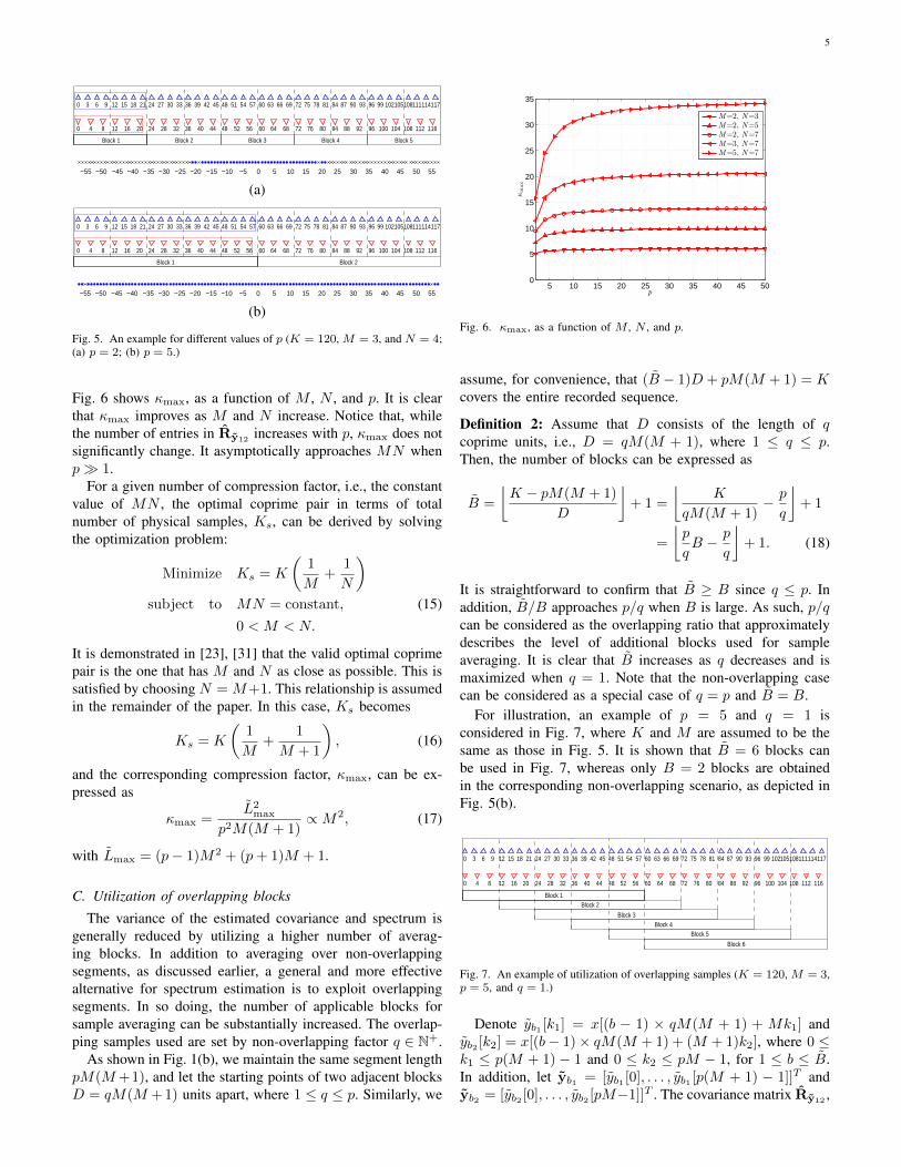
An example for different values of p is illustrated in Fig.5, where K = 120, M = 3, and N = 4 are assumed. Forthe case of p = 2, i.e., the conventional scheme, each blockforms consecutive lags within [−18, 18]. That is, Rx can bereconstructed with a maximum of dimension Lmax = 19 byaveraging B = 5 blocks. For the case of p = 5, Lmax = 55can be obtained by a consecutive lag range of [−54, 54] ineach block, whereas the number of the blocks is reduced toB = 2.

We examine the compression factor, which is defined as theratio of the number of entries in Rx over the correspondingnumber in Ry12

, expressed as

κ =L× L

pM × pN=

L2

p2MN. (13)

Because the maximum value of L is Lmax = (p − 1)MN +M +N , the maximum achievable value of κ is given by

κmax =[(p− 1)MN +M +N ]

2

p2MN. (14)

5

0 3 6 9 12 15 18 21 24 27 30 33 36 39 42 45 48 51 54 57 60 63 66 69 72 75 78 81 84 87 90 93 96 99 102105108111114117

0 4 8 12 16 20 24 28 32 36 40 44 48 52 56 60 64 68 72 76 80 84 88 92 96 100 104 108 112 116

Block 1 Block 2 Block 3 Block 4 Block 5

−55 −50 −45 −40 −35 −30 −25 −20 −15 −10 −5 0 5 10 15 20 25 30 35 40 45 50 55

(a)

0 3 6 9 12 15 18 21 24 27 30 33 36 39 42 45 48 51 54 57 60 63 66 69 72 75 78 81 84 87 90 93 96 99 102105108111114117

0 4 8 12 16 20 24 28 32 36 40 44 48 52 56 60 64 68 72 76 80 84 88 92 96 100 104 108 112 116

Block 1 Block 2

−55 −50 −45 −40 −35 −30 −25 −20 −15 −10 −5 0 5 10 15 20 25 30 35 40 45 50 55

(b)

Fig. 5. An example for different values of p (K = 120, M = 3, and N = 4;(a) p = 2; (b) p = 5.)

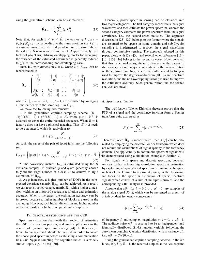
Fig. 6 shows κmax, as a function of M , N , and p. It is clearthat κmax improves as M and N increase. Notice that, whilethe number of entries in Ry12

increases with p, κmax does notsignificantly change. It asymptotically approaches MN whenp� 1.

For a given number of compression factor, i.e., the constantvalue of MN , the optimal coprime pair in terms of totalnumber of physical samples, Ks, can be derived by solvingthe optimization problem:

Minimize Ks = K

(1

M+

1

N

)subject to MN = constant, (15)

0 < M < N.

It is demonstrated in [23], [31] that the valid optimal coprimepair is the one that has M and N as close as possible. This issatisfied by choosing N = M+1. This relationship is assumedin the remainder of the paper. In this case, Ks becomes

Ks = K

(1

M+

1

M + 1

), (16)

and the corresponding compression factor, κmax, can be ex-pressed as

κmax =L2max

p2M(M + 1)∝M2, (17)

with Lmax = (p− 1)M2 + (p+ 1)M + 1.

C. Utilization of overlapping blocks

The variance of the estimated covariance and spectrum isgenerally reduced by utilizing a higher number of averag-ing blocks. In addition to averaging over non-overlappingsegments, as discussed earlier, a general and more effectivealternative for spectrum estimation is to exploit overlappingsegments. In so doing, the number of applicable blocks forsample averaging can be substantially increased. The overlap-ping samples used are set by non-overlapping factor q ∈ N+.

As shown in Fig. 1(b), we maintain the same segment lengthpM(M+1), and let the starting points of two adjacent blocksD = qM(M + 1) units apart, where 1 ≤ q ≤ p. Similarly, we

5 10 15 20 25 30 35 40 45 500

5

10

15

20

25

30

35

p

κmax

M=2, N=3

M=2, N=5

M=2, N=7

M=3, N=7

M=5, N=7

Fig. 6. κmax, as a function of M , N , and p.

assume, for convenience, that (B − 1)D + pM(M + 1) = Kcovers the entire recorded sequence.

Definition 2: Assume that D consists of the length of qcoprime units, i.e., D = qM(M + 1), where 1 ≤ q ≤ p.Then, the number of blocks can be expressed as

B =

⌊K − pM(M + 1)

D

⌋+ 1 =

⌊K

qM(M + 1)− p

q

⌋+ 1

=

⌊p

qB − p

q

⌋+ 1. (18)

It is straightforward to confirm that B ≥ B since q ≤ p. Inaddition, B/B approaches p/q when B is large. As such, p/qcan be considered as the overlapping ratio that approximatelydescribes the level of additional blocks used for sampleaveraging. It is clear that B increases as q decreases and ismaximized when q = 1. Note that the non-overlapping casecan be considered as a special case of q = p and B = B.

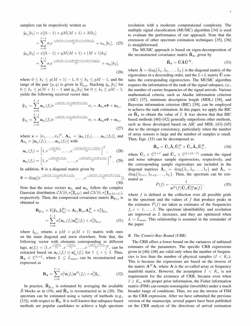
For illustration, an example of p = 5 and q = 1 isconsidered in Fig. 7, where K and M are assumed to be thesame as those in Fig. 5. It is shown that B = 6 blocks canbe used in Fig. 7, whereas only B = 2 blocks are obtainedin the corresponding non-overlapping scenario, as depicted inFig. 5(b).

0 3 6 9 12 15 18 21 24 27 30 33 36 39 42 45 48 51 54 57 60 63 66 69 72 75 78 81 84 87 90 93 96 99 102105108111114117

0 4 8 12 16 20 24 28 32 36 40 44 48 52 56 60 64 68 72 76 80 84 88 92 96 100 104 108 112 116

Block 1Block 2

Block 3Block 4

Block 5

Block 6

Fig. 7. An example of utilization of overlapping samples (K = 120, M = 3,p = 5, and q = 1.)

Denote yb1 [k1] = x[(b − 1) × qM(M + 1) + Mk1] andyb2 [k2] = x[(b− 1)× qM(M + 1) + (M + 1)k2], where 0 ≤k1 ≤ p(M + 1) − 1 and 0 ≤ k2 ≤ pM − 1, for 1 ≤ b ≤ B.In addition, let yb1 = [yb1 [0], . . . , yb1 [p(M + 1) − 1]]T andyb2 = [yb2 [0], . . . , yb2 [pM−1]]T . The covariance matrix Ry12

,

6

using the generalized scheme, can be estimated as

Ry12=

1

B

B∑b=1

yb1 yHb2 . (19)

Note that, for each 1 ≤ b ≤ B, the entries rb(k1, k2) =yb1 [k1]y∗b2 [k2] corresponding to the same position (k1, k2) incovariance matrix are still independent. As discussed above,the value of B is increased from that of B approximately by afactor of p/q. Thus, utilizing overlapping blocks for averaging,the variance of the estimated covariance is generally reducedto q/p of the corresponding non-overlapping case.

Then, Rx with dimension L×L, where L ≤ Lmax, can bereconstructed as

Rx =

ˆr[0] ˆr[−1] . . . ˆr[−L+ 1]ˆr[1] ˆr[0] . . . ˆr[−L+ 2]

...... . . .

...ˆr[L− 2] ˆr[L− 3] . . . ˆr[−1]ˆr[L− 1] ˆr[L− 2] . . . ˆr[0]

, (20)

where ˆr[τ ], τ = −L+1, . . . , L−1, are estimated by averagingall the entries with the same lag τ in Ry12

.We make the following two remarks:1. In the generalized coprime sampling scheme, (B −

1)qM(M + 1) + pM(M + 1) = K, where p, q ∈ N+, isassumed to cover the entire recorded sequence. When B = 1,factor q does not have a physical meaning. Thus, B ≥ 2 needsto be guaranteed, which is equivalent to

p+ q ≤ K

M(M + 1). (21)

As such, the range of the pair of (p, q) falls into the followingset,

Πp,q =

{(p, q) | p+ q ≤ K

M(M + 1), 1 ≤ q ≤ p, p, q ∈ N+

}.

(22)2. The covariance matrix Ry12

is estimated using the Bavailable samples. In practice, p and q are generally chosento yield the large number of blocks B to achieve to rigidestimation of Ry12 .

3. As p increases, a higher number of DOFs in the com-pressed covariance matrix Ry12

can be achieved. As a result,we can reconstruct covariance matrix Rx with a higher dimen-sion, yielding an improved spectrum resolution and estimationaccuracy. When q increases, the estimation accuracy can beimproved because a higher number of blocks are used in theaveraging. However, such higher dimension and higher numberof blocks result in a higher computational complexity.

IV. SPECTRUM ESTIMATION AND THE CRB

Spectrum estimation deals with the problem of estimatingthe PSD of a random process, and finds applications in thecontext of dynamic spectrum sharing [24]. In this case, abroad frequency band should be sensed in order to locatethe unoccupied spectrum before establishing a communicationlink. Sub-Nyquist sampling for cognitive radios is a widelystudied topic, e.g., in [25]–[30].

Generally, power spectrum sensing can be classified intotwo major categories. The first category reconstructs the signalwaveforms and then estimate the power spectrum, whereas thesecond category estimates the power spectrum from the signalcovariance, i.e., the second-order statistics. The approachdiscussed in [25]–[27] belongs to the former where the signalsare assumed to be sparse in some domain and sub-Nyquistsampling is implemented to recover the signal waveformsthrough compressive sensing. The approach adopted in thispaper, along with [28]–[30] and several other references [11]–[13], [15], [16] belong to the second category. Note, however,that this paper makes significant difference to the papers inits category, as our major contribution is the generalizationof the coprime sampling, where the multiple unit factor p isused to improve the degrees-of-freedom (DOFs) and spectrumresolution, and the non-overlapping factor q is used to improvethe estimation accuracy. Such generalization and the relatedanalyses are novel.

A. Spectrum estimation

The well-known Wiener-Khinchin theorem proves that thePSD of a signal and the covariance function form a Fouriertransform pair, expressed as

P [f ] =

∞∑τ=−∞

r[τ ]e−j2πτf/fs . (23)

Therefore, once Rx is reconstructed, then P [f ] can be esti-mated by employing the discrete Fourier transform which doesnot require the assumptions of signal sparsity in the frequencydomain. The applicability to continuous spectrum signals willbe demonstrated using a simulation example in Section V.

For signals with sparse and discrete spectrum, however,we can further achieve high-resolution spectrum estimationby exploiting subspace-based spectrum estimation techniques,in lieu of the Fourier transform. As such, in the following,we focus on the spectrum estimation of sparse spectrumsignals which consist of a sum of multiple sinusoids, and thecorresponding CRB analysis is provided.

Assume that x[k], for k = 0, 1, . . . ,K − 1, are samples ofthe analog signal X(t), which can be presented as a sum ofI independent frequency components

x[k] =

I−1∑i=0

σie−j2πkfi

fs + n[k], (24)

of frequency fi and complex magnitudes σi, i = 0, . . . , I − 1.The additive noise n[k] is assumed to be an independent andidentically distributed (i.i.d.) random variable following thezero-mean complex Gaussian distribution with a variance σ2

n,i.e., n[k] ∼ CN (0, σ2

n).Using the generalized coprime sampling scheme, in the bth

block, 0 ≤ b ≤ B−1, the received outputs at the two coprime

7

samplers can be respectively written as

yb1 [k1] = x[(b− 1)× qM(M + 1) +Mk1]

=

I−1∑i=0

σie−j2π[(b−1)×qM(M+1)+Mk1]fi

fs + nb1 [k1], (25)

yb2 [k2] = x[(b− 1)× qM(M + 1) + (M + 1)k2]

=

I−1∑i=0

σie−j2π[(b−1)×qM(M+1)+(M+1)k2]fi

fs + nb2 [k2],

(26)

where 0 ≤ k1 ≤ p(M + 1) − 1, 0 ≤ k2 ≤ pM − 1, and therange of the pair (p, q) is given in Πp,q . Stacking yb1 [k1] for0 ≤ k1 ≤ p(M + 1) − 1 and yb2 [k2] for 0 ≤ k2 ≤ pM − 1,yields the following received vector data

yb1 =

I−1∑i=0

ab1(fi)e−j2π[(b−1)×qM(M+1)]fi

fs σi = Ab1sΦ + nb1 ,

yb2 =

I−1∑i=0

ab2(fi)e−j2π[(b−1)×qM(M+1)]fi

fs σi = Ab2sΦ + nb2 ,

(27)

where s = [σ1, . . . , σI ]T , Ab1 = [ab1(f1), . . . ,ab1(fI)], and

Ab2 = [ab2(f1), . . . ,ab2(fI)] with

ab1(fi) =[1, e

−j2πMfifs , . . . , e

−j2π[p(M+1)−1]Mfifs

]T, (28)

ab2(fi) =[1, e

−j2π(M+1)fifs , . . . , e

−j2π(pM−1)(M+1)fifs

]T. (29)

In addition, Φ is a diagonal matrix given by

Φ = diag([e−j2π[(b−1)×qM(M+1)]f1

fs , . . . , e−j2π[(b−1)×qM(M+1)]fI

fs ]).(30)

Note that the noise vectors nb1 and nb2 follow the complexGaussian distribution CN (0, σ2

nIpM ) and CN (0, σ2nIp(M+1)),

respectively. Then, the compressed covariance matrix Ry12is

obtained as

Ry12= E[yb1 y

Hb2 ] = Ab1RssA

Hb2 + σ2

niy12

=

I−1∑i=0

σ2i ab1(fi)a

Hb2(fi) + σ2

niy12 , (31)

where iy12 returns a pM × p(M + 1) matrix with oneson the main diagonal and zeros elsewhere. Note that, thefollowing vector with elements corresponding to differentlags, a(fi) = [1, e

−j2πfifs , e

−j4πfifs , . . . , e

−j2(L−1)πfifs ]T , can be

extracted based on ab1(fi) ⊗ a∗b2(fi) for 1 ≤ i ≤ I . Thus,Rx ∈ CL×L, where L ≤ Lmax, can be reconstructed andexpressed as

Rx =

I−1∑i=0

σ2i a(fi)a

H(fi) + σ2nIL. (32)

In practice, Ry12 is estimated by averaging the availableB blocks as in (19), and Rx is reconstructed as in (20). Thespectrum can be estimated using a variety of methods (e.g.,[33]), with respect to Rx. It is well known that subspace-basedmethods are popular candidates to achieve a high spectrum

resolution with a moderate computational complexity. Themultiple signal classification (MUSIC) algorithm [34] is usedto evaluate the performance of our approach. Note that theextension of other spectrum estimation techniques [35], [36]is straightforward.

The MUSIC approach is based on eigen-decomposition ofthe reconstructed covariance matrix Rx, given by

Rx = UΛUH , (33)

where Λ = diag{λ1, λ2, . . . , λL} is the diagonal matrix of theeigenvalues in a descending order, and the L×L matrix U con-tains the corresponding eigenvectors. The MUSIC algorithmrequires the information of the rank of the signal subspace, i.e.,the number of carrier frequencies of the signal arrivals. Variousmathematical criteria, such as Akaike information criterion(AIC) [37], minimum description length (MDL) [38], andBayesian information criterion (BIC) [39], can be employedto achieve the rank estimation. In this paper, we apply the BICon Rx to obtain the value of I . It was shown that that BICbased methods [40]–[42] generally outperform other methods,such as those developed based on AIC and MDL [43]–[45]due to the stronger consistency, particularly when the numberof array sensors is large and the number of samples is small.Then, Eqn. (33) can be decomposed as

Rx = UsΛsUHs + UnΛnUH

n , (34)

where Us ∈ CL×I and Un ∈ CL×(L−I) contain the signaland noise subspace sample eigenvectors, respectively, andthe corresponding sample eigenvalues are included in thediagonal matrices Λs = diag{λ1, λ2, . . . , λI} and Λn =diag{λI+1, λI+2, . . . , λL}. Then, the spectrum can be esti-mated as

P (f) =1

aH(f)UnUHn a(f)

, (35)

where f is defined as the collection over all possible gridsin the spectrum and the values of f that produce peaks inthe estimator P (f) are taken as estimates of the frequenciesfi, i = 1, . . . , I . The spectrum identifiability and resolutionare improved as L increases, and they are optimized whenL = Lmax. This relationship is assumed in the remainder ofthe paper.

B. The Cramer-Rao Bound (CRB)

The CRB offers a lower bound on the variances of unbiasedestimates of the parameters. The specific CRB expressionsgiven in [46]–[48] are valid only when the number of frequen-cies is less than the number of physical samples (I < Ks).This is because the expressions are based on the inverse ofthe matrix AHA, where A is the so-called array or frequencymanifold matrix. However, the assumption I < Ks is notrequirement for the existence of CRB, because even whenI ≥ Ks, with proper prior information, the Fisher informationmatrix (FIM) can remain nonsingular (invertible) under a muchbroader range of conditions. Thus, we use the inverse of FIMas the CRB expression. After we have submitted the previousversion of the manuscript, several papers have been publishedon the CRB analysis of the directions of arrival estimation

8

when more sources than the number of sensors are handledin the context of coarrays. We have cited these papers asreferences [49]–[51]. However, none of these papers providerevealing solutions in a compact matrix form.

For a set of vectors yb = [yTb1 yTb2 ]T , b = 1, . . . , B,the CRB is calculated by the well-known expression [47]involving the FIM elements

Fαiαj = BTr

{R−1y

∂Ry

∂αiR−1y

∂Ry

∂αj

}, (36)

for unknown variables αi and αj , where Ry is expressed as

Ry = E[ybyHb ] =

I−1∑i=0

σ2i ab(fi)a

Hb (fi) + σ2

nIp(2M+1), (37)

and ab(fi) = [aTb1(fi) aTb2(fi)]T .

In the underlying case, the unknown parameters are the Isignal frequencies fi and powers σ2

i for i = 1, . . . , I , as wellas the noise power σ2

n. Therefore, the elements in the (2I +1)× (2I + 1) Fisher matrix F can be written in terms of theblock matrices, for i, j = 1, . . . , I , given by

Fi,j = BTr

{R−1y

∂Ry

∂fiR−1y

∂Ry

∂fj

},

Fi,j+I = BTr

{R−1y

∂Ry

∂fiR−1y

∂Ry

∂σ2j

},

Fi,2I+1 = BTr

{R−1y

∂Ry

∂fiR−1y

∂Ry

∂σ2n

},

Fi+I,j = BTr

{R−1y

∂Ry

∂σ2i

R−1y

∂Ry

∂fj

},

Fi+I,j+I = BTr

{R−1y

∂Ry

∂σ2i

R−1y

∂Ry

∂σ2j

},

Fi+I,2I+1 = BTr

{R−1y

∂Ry

∂σ2i

R−1y

∂Ry

∂σ2n

},

F2I+1,2I+1 = BTr

{R−1y

∂Ry

∂σ2n

R−1y

∂Ry

∂σ2n

}, (38)

where

∂Ry

∂fi= σ2

i

[∂ab(fi)

∂fiaHb (fi) + ab(fi)

∂aHb (fi)

∂fi

],

∂Ry

∂σ2i

= ab(fi)aHb (fi),

∂Ry

∂σ2n

= Ip(2M+1). (39)

Then, the CRB of estimated frequencies is obtained as

CRB(fi) =[F−1

]i,i. (40)

V. SIMULATION RESULTS

For illustrative purposes, we demonstrate the spectrum esti-mation performance under different choices of the argumentswithin the generalized coprime sampling scheme. Assume thatI frequency components with identical powers are distributedin the frequency band [−500, 500] MHz. Assume that K =50000 samples are generated with a Nyquist sampling ratefs=1 GHz. In addition, the noise power is assumed to be

identical across the entire spectrum. The MUSIC method isused to estimate the power spectrum. Our benchmarks are thespectrum DOFs and their statistical performance. The latter isevaluated in terms of average relative root mean square error(RMSE) of the estimated frequencies, defined as

Relatvie RMSE(fi) =1

fs

√√√√ 1

500I

500∑n=1

I∑i=1

(fi(n)− fi)2,

(41)where fi(n) is the estimate of fi from the nth Monte Carlotrial, n = 1, . . . , 500.

A. The performance of coprime sampling

We first illustrate the performance of coprime sampling.Herein, the conventional coprime sampling scheme is consid-ered, i.e., p = 2. In addition, M = 3 is assumed. As such, theL× L = 19× 19 covariance matrix Rx can be reconstructedfrom Ry12

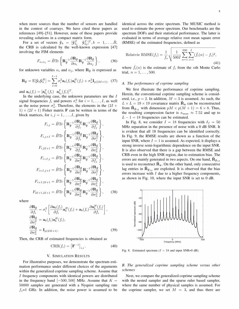
with dimension pM × p(M + 1) = 6 × 8. Thus,the resulting compression factor is κmax ≈ 7.52 and up toL− 1 = 18 frequencies can be estimated.

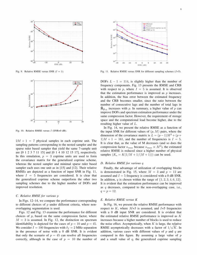
In Fig. 8, we consider I = 18 frequencies with δf = 50MHz separation in the presence of noise with a 0 dB SNR. Itis evident that all 18 frequencies can be identified correctly.In Fig. 9, the RMSE results are shown as a function of theinput SNR, where I = 1 is assumed. As expected, it displays astrong inverse semi-logarithmic dependence on the input SNR.It is also observed that there is a gap between the RMSE andCRB even in the high SNR region, due to estimation bias. Theerrors are mainly generated in two aspects. On one hand, Ry12

is used to reconstruct Rx. On the other hand, only consecutivelag entries in Ry12 are exploited. It is observed that the biaserrors increase with I due to a higher frequency components,as shown in Fig. 10, where the input SNR is set to 0 dB.

−500 0 500−120

−100

−80

−60

−40

−20

0

Frequency (MHz)

Nor

mal

ized

spe

ctru

m (

dB)

Fig. 8. Estimated spectrum (I = 18 and input SNR=0 dB).

B. The generalized coprime sampling scheme versus otherschemes

Next, we compare the generalized coprime sampling schemewith the nested sampler and the sparse ruler based sampler,where the same number of physical samples is assumed. Forthe coprime sampler, we set M = 3, and thus there are

9

−20 −10 0 10 2010

−6

10−5

10−4

10−3

10−2

SNR (dB)

Relative

RMSE

EstCRB

Fig. 9. Relative RMSE versus SNR (I = 1).

0 5 10 15 2010

−5

10−4

10−3

10−2

I

RelativeRMSE

EstCRB

Fig. 10. Relative RMSE versus I (SNR=0 dB).

2M + 1 = 7 physical samples in each coprime unit. Thesampling patterns corresponding to the nested sampler and thesparse ruler based sampler that yield the same 7-sample unitare [0 1 2 3 7 11 15] and [0 1 4 10 12 15 17], respectively.In this simulation, p = 3 coprime units are used to formthe covariance matrix for the generalized coprime scheme,whereas the nested sampler and minimal sparse ruler basedsampler each uses one unit as in [15] and [12]. Their relativeRMSEs are depicted as a function of input SNR in Fig. 11,where I = 5 frequencies are considered. It is clear thatthe generalized coprime scheme outperform the other twosampling schemes due to the higher number of DOFs andimproved resolution.

C. Relative RMSE for various p

In Figs. 12–14, we compare the performance correspondingto different choices of p under different criteria, where non-overlapping segmentation is used.

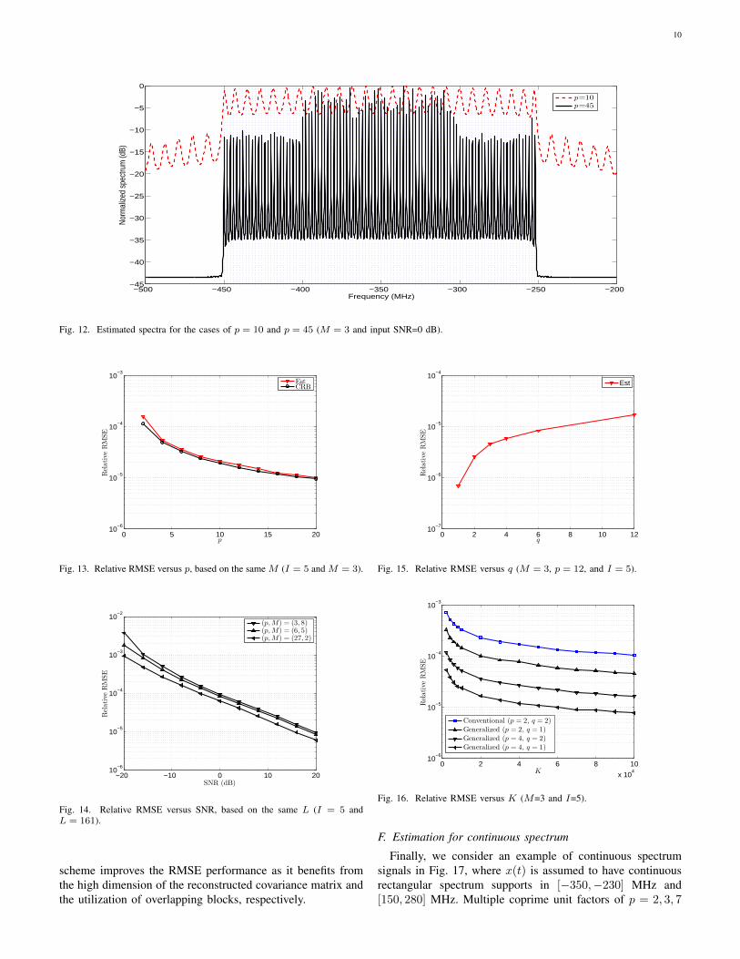
Figs. 12 and Fig. 13 examine the performance for differentchoices of p, based on the same compression factor, whereM = 3 is assumed. In Fig. 12, the distinction on spectrumidentifiability is depicted for the cases of p = 10 and p = 45.We consider I = 100 frequencies with δf = 2 MHz separationin the presence of noise with a 0 dB SNR. It is evidentthat only the scenario of p = 45 can resolve all frequenciescorrectly, although in the case of p = 10 the number of

-20 -15 -10 -5 0 5 10 15 20SNR (dB)

10-6

10-5

10-4

10-3

10-2

10-1

RelativeRMSE

Minimal

Nested

Generalized coprime (p=3)

CRB (p=3)

Fig. 11. Relative RMSE versus SNR for different sampling schemes (I=5).

DOFs L − 1 = 114, is slightly higher than the number offrequency components. Fig. 13 presents the RMSE and CRBwith respect to p, where I = 5 is assumed. It is observedthat the estimation performance is improved as p increases.In addition, the bias error between the estimated frequencyand the CRB becomes smaller, since the ratio between thenumber of consecutive lags and the number of total lags inRy12

increases with p. In summary, a higher value of p canimprove DOFs and spectrum estimation performance under thesame compression factor. However, the requirement of storagespace and the computational load become higher, due to theresulting higher value of L.

In Fig. 14, we present the relative RMSE as a function ofthe input SNR for different values of (p,M) pairs, where thedimension of the covariance matrix is L = (p− 1)M2 + (p+1)M + 1 = 161, and the number of frequencies is I = 5.It is clear that, as the value of M decreases (and so does thecompression factor κmax because κmax ∝M2), the estimatedrelative RMSE is reduced since a higher number of physicalsamples (Ks = K(1/M + 1/(M + 1))) can be used.

D. Relative RMSE for various q

Finally, the advantage of utilization of overlapping blocksis demonstrated in Fig. 15, where M = 3 and p = 12 areassumed and I = 5 frequency is considered with a 0 dB SNR.In addition, q is chosen within the range of {1, 2, 3, 4, 6, 12}.It is evident that the estimation performance can be improvedas q decreases, compared to the non-overlapping case, i.e.,q = p = 12.

E. Relative RMSE versus K

In Fig. 16, we present the relative RMSE performance withrespect to K, where M=3 is assumed, and I=5 frequencieswith a 0 dB input SNR are considered. It is evident thatthe estimated relative RMSE performance is improved as Kincreases because a higher number of blocks is used to reducethe noise effect. Asymptotically, when K is large, the relativeRMSE asymptotically decreases with a factor of 1/

√K. In

addition, various cases with different values of p and q arecompared in this figure. By assuming a large value of pand a small value of q, the generalized coprime sampling

10

−500 −450 −400 −350 −300 −250 −200−45

−40

−35

−30

−25

−20

−15

−10

−5

0

Frequency (MHz)

Norm

alize

d sp

ectru

m (d

B)

p=10

p=45

Fig. 12. Estimated spectra for the cases of p = 10 and p = 45 (M = 3 and input SNR=0 dB).

0 5 10 15 2010

−6

10−5

10−4

10−3

p

RelativeRMSE

EstCRB

Fig. 13. Relative RMSE versus p, based on the same M (I = 5 and M = 3).

−20 −10 0 10 2010

−6

10−5

10−4

10−3

10−2

SNR (dB)

Relative

RMSE

(p,M) = (3, 8)(p,M) = (6, 5)(p,M) = (27, 2)

Fig. 14. Relative RMSE versus SNR, based on the same L (I = 5 andL = 161).

scheme improves the RMSE performance as it benefits fromthe high dimension of the reconstructed covariance matrix andthe utilization of overlapping blocks, respectively.

0 2 4 6 8 10 1210

−7

10−6

10−5

10−4

q

RelativeRMSE

Est

Fig. 15. Relative RMSE versus q (M = 3, p = 12, and I = 5).

0 2 4 6 8 10

x 104

10−6

10−5

10−4

10−3

K

Relative

RMSE

Conventional (p = 2, q = 2)Generalized (p = 2, q = 1)

Generalized (p = 4, q = 2)Generalized (p = 4, q = 1)

Fig. 16. Relative RMSE versus K (M=3 and I=5).

F. Estimation for continuous spectrum

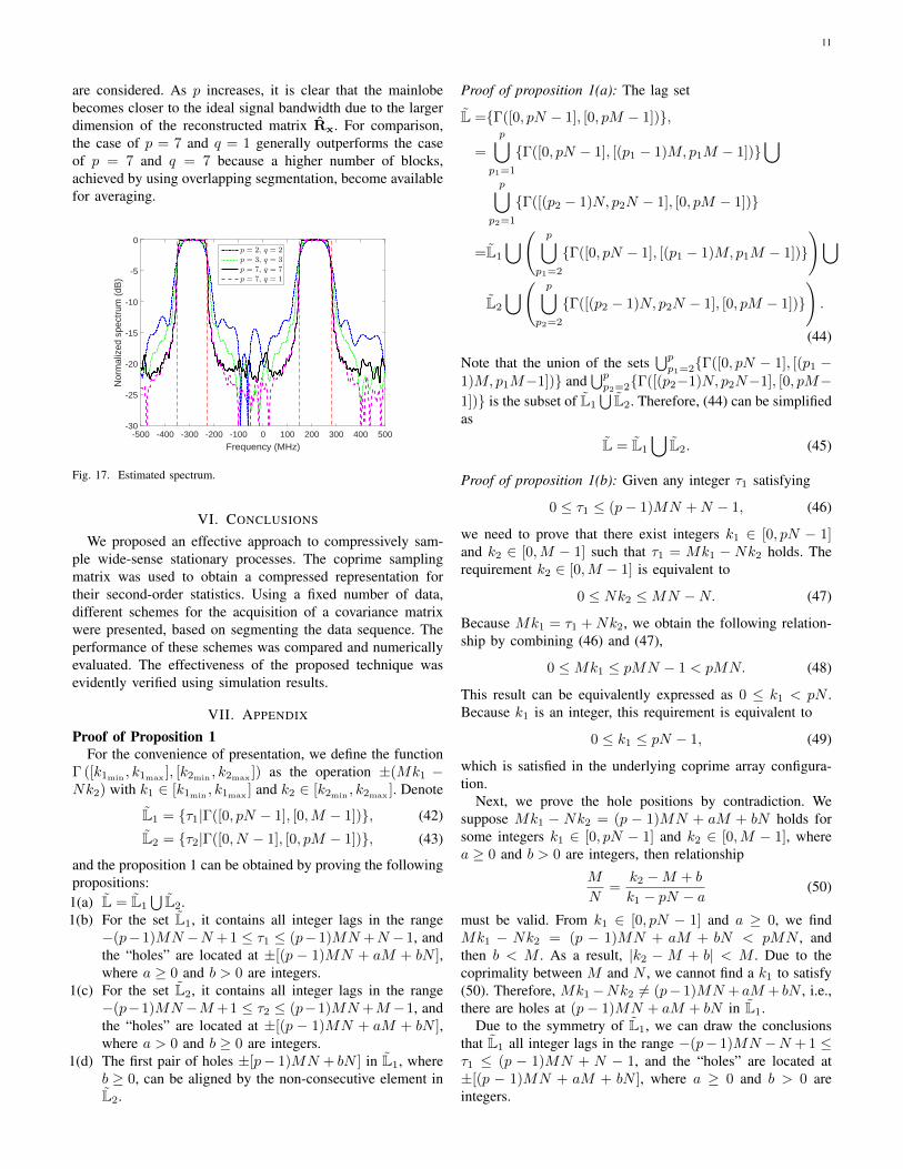
Finally, we consider an example of continuous spectrumsignals in Fig. 17, where x(t) is assumed to have continuousrectangular spectrum supports in [−350,−230] MHz and[150, 280] MHz. Multiple coprime unit factors of p = 2, 3, 7

11

are considered. As p increases, it is clear that the mainlobebecomes closer to the ideal signal bandwidth due to the largerdimension of the reconstructed matrix Rx. For comparison,the case of p = 7 and q = 1 generally outperforms the caseof p = 7 and q = 7 because a higher number of blocks,achieved by using overlapping segmentation, become availablefor averaging.

-500 -400 -300 -200 -100 0 100 200 300 400 500

Frequency (MHz)

-30

-25

-20

-15

-10

-5

0

Nor

mal

ized

spe

ctru

m (

dB)

p = 2, q = 2

p = 3, q = 3

p = 7, q = 7

p = 7, q = 1

Fig. 17. Estimated spectrum.

VI. CONCLUSIONS

We proposed an effective approach to compressively sam-ple wide-sense stationary processes. The coprime samplingmatrix was used to obtain a compressed representation fortheir second-order statistics. Using a fixed number of data,different schemes for the acquisition of a covariance matrixwere presented, based on segmenting the data sequence. Theperformance of these schemes was compared and numericallyevaluated. The effectiveness of the proposed technique wasevidently verified using simulation results.

VII. APPENDIX

Proof of Proposition 1For the convenience of presentation, we define the function

Γ ([k1min, k1max

], [k2min, k2max

]) as the operation ±(Mk1 −Nk2) with k1 ∈ [k1min

, k1max] and k2 ∈ [k2min

, k2max]. Denote

L1 = {τ1|Γ([0, pN − 1], [0,M − 1])}, (42)

L2 = {τ2|Γ([0, N − 1], [0, pM − 1])}, (43)

and the proposition 1 can be obtained by proving the followingpropositions:1(a) L = L1

⋃L2.

1(b) For the set L1, it contains all integer lags in the range−(p− 1)MN −N + 1 ≤ τ1 ≤ (p− 1)MN +N − 1, andthe “holes” are located at ±[(p − 1)MN + aM + bN ],where a ≥ 0 and b > 0 are integers.

1(c) For the set L2, it contains all integer lags in the range−(p−1)MN −M +1 ≤ τ2 ≤ (p−1)MN +M −1, andthe “holes” are located at ±[(p − 1)MN + aM + bN ],where a > 0 and b ≥ 0 are integers.

1(d) The first pair of holes ±[p− 1)MN + bN ] in L1, whereb ≥ 0, can be aligned by the non-consecutive element inL2.

Proof of proposition 1(a): The lag set

L ={Γ([0, pN − 1], [0, pM − 1])},

=

p⋃p1=1

{Γ([0, pN − 1], [(p1 − 1)M,p1M − 1])}⋃

p⋃p2=1

{Γ([(p2 − 1)N, p2N − 1], [0, pM − 1])}

=L1

⋃(p⋃

p1=2

{Γ([0, pN − 1], [(p1 − 1)M,p1M − 1])}

)⋃L2

⋃(p⋃

p2=2

{Γ([(p2 − 1)N, p2N − 1], [0, pM − 1])}

).

(44)

Note that the union of the sets⋃pp1=2{Γ([0, pN − 1], [(p1 −

1)M,p1M−1])} and⋃pp2=2{Γ([(p2−1)N, p2N−1], [0, pM−

1])} is the subset of L1

⋃L2. Therefore, (44) can be simplified

as

L = L1

⋃L2. (45)

Proof of proposition 1(b): Given any integer τ1 satisfying

0 ≤ τ1 ≤ (p− 1)MN +N − 1, (46)

we need to prove that there exist integers k1 ∈ [0, pN − 1]and k2 ∈ [0,M − 1] such that τ1 = Mk1 − Nk2 holds. Therequirement k2 ∈ [0,M − 1] is equivalent to

0 ≤ Nk2 ≤MN −N. (47)

Because Mk1 = τ1 +Nk2, we obtain the following relation-ship by combining (46) and (47),

0 ≤Mk1 ≤ pMN − 1 < pMN. (48)

This result can be equivalently expressed as 0 ≤ k1 < pN .Because k1 is an integer, this requirement is equivalent to

0 ≤ k1 ≤ pN − 1, (49)

which is satisfied in the underlying coprime array configura-tion.

Next, we prove the hole positions by contradiction. Wesuppose Mk1 − Nk2 = (p − 1)MN + aM + bN holds forsome integers k1 ∈ [0, pN − 1] and k2 ∈ [0,M − 1], wherea ≥ 0 and b > 0 are integers, then relationship

M

N=

k2 −M + b

k1 − pN − a(50)

must be valid. From k1 ∈ [0, pN − 1] and a ≥ 0, we findMk1 − Nk2 = (p − 1)MN + aM + bN < pMN , andthen b < M . As a result, |k2 − M + b| < M . Due to thecoprimality between M and N , we cannot find a k1 to satisfy(50). Therefore, Mk1−Nk2 6= (p− 1)MN + aM + bN , i.e.,there are holes at (p− 1)MN + aM + bN in L1.

Due to the symmetry of L1, we can draw the conclusionsthat L1 all integer lags in the range −(p− 1)MN −N + 1 ≤τ1 ≤ (p − 1)MN + N − 1, and the “holes” are located at±[(p − 1)MN + aM + bN ], where a ≥ 0 and b > 0 areintegers.

12

Proof of proposition 1(c): We omit the proof of proposition1(c), which can be proved by using the same method as in theproof of proposition 1(b).

Proof of proposition 1(d): Based on the proposition 1(b), thereare holes (p − 1)MN + aM + bN in L1, where a ≥ 0 andb > 0 are integers. If the holes are aligned by the elements inL2, the following relationship

(p− 1)MN + aM + bN = ±(Mk1 −Nk2) (51)

must be valid for k1 ∈ [0, N − 1] and k2 ∈ [0, pM − 1]. Therequirement is equivalent to

(p− 1)MN + aM + (b+ k2)N = Mk1,

or(p− 1)MN + (a+ k1)M + bN = Nk2,

i.e.,b = −k2, or a = −k1. (52)

It is only possible for a = k1 = 0 when k1 ∈ [0, N − 1],k2 ∈ [0, pM − 1], a ∈ [0,∝), and b ∈ (0,∝). Then, therequirement further becomes

(p− 1)M + b = k2. (53)

In the proof of proposition 1(b), it is shown that b < M , i.e.,b ≤M−1. As such, k2 ∈ ((p− 1)M,pM − 1] ⊆ [0, pM−1].Therefore, the holes (p−1)MN+bN(a = 0) in L1 are alignedby the element in L2 for some integers k2 ∈ [0, pM − 1].As a result, the first hole outside the consecutive range of Lbecomes (p− 1)MN +M +N . Then, the set L contains allinteger lags in the range

−(p−1)MN −M −N +1 ≤ τ ≤ (p−1)MN +M +N −1.(54)

REFERENCES

[1] S. Qin, Y. D. Zhang, and M. G. Amin, “High-resolutionfrequency estimation using generalized coprime sampling,” inProc. SPIE Mobile, Multimedia/Image Process., Secur. Appl.Conf. (SPIE), Baltimore, MD, 2015, vol. 9497, pp. 94970K1–94970K7.

[2] S. Qin, Y. D. Zhang, M. G. Amin, and A. M. Zoubir, “Gener-alized coprime sampling of Toeplitz matrices,” in Proc. IEEEInt. Conf. Acoust. Speech Signal Process. (ICASSP), Shanghai,China, 2016, pp. 4468–4472.

[3] E. J. Candes, J. Romberg, and T. Tao, “Robust uncertaintyprinciples: exact signal reconstruction from highly incompletefrequency information,” IEEE Trans. Inf. Theory, vol. 52, no. 2,pp. 489–509, 2006.

[4] D. L. Donoho, “Compressed sensing,” IEEE Trans. Inf. Theory,vol. 52, no. 4, pp. 1289–1306, 2006.

[5] J. A. Tropp and A. C. Gilbert, “Signal recovery from randommeasurements via orthogonal matching pursuit,” IEEE Trans.Inf. Theory, vol. 53, no. 12, pp. 4655–4666, 2007.

[6] R. Tibshirani, “Regression shrinkage and selection via the lasso,”J. R. Stat. Soc., Ser. B, vol. 58, no. 1, pp. 267–288, 1996.

[7] S. Ji, D. Dunson, and L. Carin, “Multitask compressive sensing,”IEEE Trans. Signal Process., vol. 57, no. 1, pp. 92–106, 2009.

[8] Q. Wu, Y. D. Zhang, M. G. Amin, and B. Himed, “Multi-taskBayesian compressive sensing exploiting intra-task dependency,”IEEE Signal Process. Lett., vol. 22, no. 4, pp. 430–434, 2015.

[9] G. Dasarathy, P. Shah, B. N. Bhaskar, and R. Nowak, “Sketchingsparse matrices, covariances, and graphs via tensor products,”IEEE Trans. Inf. Theory, vol. 61, no. 3, pp. 1373–1388, 2015.

[10] Y. Chen, Y. Chi, and A. Goldsmith, “Exact and stable covarianceestimation from quadratic sampling via convex programming,”IEEE Trans. Inf. Theory, vol. 61, no. 7, pp. 4034–4059, 2015.

[11] G. Leus and Z. Tian, “Recovering second-order statistics fromcompressive measurements,” in Proc. IEEE Int. Workshop onComp. Adv. in Multi-Sensor Adaptive Process. (CAMSAP), SanJuan, Puerto Rico, 2011, pp. 337–340.

[12] D. D. Ariananda and G. Leus, “Compressive wideband powerspectrum estimation,” IEEE Trans. Signal Process., vol. 60, no.9, pp. 4775–4789, 2012.

[13] D. Romero and G. Leus, “Compressive covariance sampling,” inProc. Inf. Theory Appl. Workshop (ITA), San Diego, CA, 2013,pp. 1–8.

[14] C. L. Nikias and J. M. Mendel, “Signal processing with higher-order spectra,” IEEE Signal Process. Mag., vol. 10, no. 3, pp.10–37, 1993.

[15] H. Qiao and P. Pal, “Generalized nested sampling for com-pression and exact recovery of symmetric Toeplitz matrices,”in Proc. IEEE Global Conf. Signal Inf. Process. (GlobalSIP),Atlanta, GA, 2014, pp. 443–447.

[16] Z. Tian, Y. Tafesse, and B. M. Sadler, “Cyclic feature detectionwith sub-Nyquist sampling for wideband spectrum sensing,”IEEE J. Sel. Top. Signal Process., vol. 6, no. 1, pp. 58–69, 2012.

[17] P. P. Vaidyanathan and P. Pal, “Sparse sensing with co-primesamplers and arrays,” IEEE Trans. Signal Process., vol. 59, no.2, pp. 573–586, 2011.

[18] P. Pal and P. P. Vaidyanathan, “Nested arrays: A novel approachto array processing with enhanced degrees of freedom,” IEEETrans. Signal Process., vol. 58, no. 8, pp. 4167–4181, 2010.

[19] M. A. Lexa, M. E. Davis, J. S. Thompson, and J. Nikolic,“Compressive power spectral density estimation,” in Proc. IEEEInt. Conf. Acoust. Speech Signal Process. (ICASSP), Prague,Czech Republic, 2011, pp. 3884–3887.

[20] Y. L. Polo, Y. Wang, A. Pandharipande, and G. Leus, “Com-pressive wide-band spectrum sensing,” in Proc. IEEE Int. Conf.Acoust. Speech Signal Process. (ICASSP), Taipei, Taiwan, 2009,pp. 2337–2340.

[21] D. D. Ariananda, G. Leus, and Z. Tian, “Multi-coset samplingfor power spectrum blind sensing,” in Proc. Int. Conf. Digit.Signal Process. (DSP), Corfu, Greece, 2011, pp. 1–8.

[22] P. D. Welch, “The use of fast Fourier transform for the es-timation of power spectra: a method based on time-averagingover short, modified periodograms,” IEEE Trans. Audio Elec-troacoust., vol. 15, no. 2, pp. 70–73, 1967.

[23] S. Qin, Y. D. Zhang, and M. G. Amin, “Generalized coprimearray configurations for direction-of-arrival estimation,” IEEETrans. Signal Process., vol. 63, no. 6, pp. 1377–1390, 2015.

[24] Q. Zhao and B. M. Sadler, “A survey of dynamic spectrumaccess,” IEEE Signal Process. Mag., vol. 24, no. 3, pp. 79–89,2007.

[25] M. Mishali and Y. Eldar, “From theory to practice: Sub-Nyquistsampling of sparse wideband analog signals,” IEEE J. Sel. Top.Signal Process., vol. 4, no. 2, pp. 375–391, 2010.

[26] R. Venkataramani and Y. Bresler, “Perfect reconstruction for-mulas and bound on aliasing error in sub-Nyquist nonuniformsampling of multiband signals,” IEEE Trans. Inf. Theory, vol.46, no. 6, pp. 2173–2183, 2000.

[27] M. Mishali and Y. Eldar, “Blind multiband signal reconstruc-

13

tion: Compressed sensing for analog signals,” IEEE Trans.Signal Process., vol. 57, no. 3, pp. 993–1009, 2009.

[28] H. Sun, W. Y. Chiu, J. Jiang, A. Nallanathan and H. V. Poor,“Wideband spectrum sensing with sub-Nyquist sampling incognitive radios,” IEEE Trans. Signal Process., vol. 60, no. 11,pp. 6068–6073, 2012.

[29] D. Cohen and Y. C. Eldar, “Sub-Nyquist sampling for powerspectrum sensing in cognitive radios: A unified approach,” IEEETrans. Signal Process., vol. 62, no. 15, pp. 3897–3910, 2014.

[30] M. Shaghaghi and S. A. Vorobyov, “Finite–lengthand asymptotic analysis of averaged correlogram forundersampled data,” Appl. Comput. Harmon. Anal.,http://dx.doi.org/10.1016/j.acha.2016.02.001.

[31] K. Adhikari, J. R. Buck and K. E. Wage, “Extending coprimesensor arrays to achieve the peak side lobe height of a fulluniform linear array,” EURASIP J. Wireless Commun. Netw.,doi:10.1186/1687–6180–2014–148, 2014.

[32] P. Stoica and A. Nehorai, “MUSIC, maximum likelihood,and Cramer-Rao bound,” IEEE Trans. Acoust. Speech SignalProcess., vol. 37, no. 5, pp. 720–741, 1989.

[33] P. Stoica and R. L. Moses, Spectrum Analysis of Signals, UpperSaddle River, NJ: Prentice-Hall, 2005.

[34] R. Schmidt, “Multiple emitter location and signal parameterestimation,” IEEE Trans. Antennas Propag., vol. 34, no. 3, pp.276–280, 1986.

[35] R. Roy and T. Kailath, “ESPRIT – Estimation of signal param-eters via rotation invariance techniques,” IEEE Trans. Acoust.Speech Signal Process., vol. 17, no. 7, pp. 984–995, 1989.

[36] Y. Hua and T. K. Sarkar, “Matrix pencil method for estimatingparameters of exponentially damped/undamped sinusoids innoise,” IEEE Trans. Acoust. Speech Signal Process., vol. 38,no. 5, pp. 814–824, 1990.

[37] H. Akaike, “A new look at the statistical model identification,”IEEE Trans. Autom. Control, vol. 19, no. 6, pp. 716–723, 1974.

[38] M. Wax and T. Kailath, “Detection of signals by informationtheoretic criteria,” IEEE Trans. Acoust. Speech Signal Process.,vol. 33, no. 2, pp. 387–392, 1985.

[39] G. Schwarz, “Estimating the dimension of a model,” Ann.Statist., vol. 6, no. 2, pp. 461–464, 1978.

[40] Z. Lu and A. M. Zoubir, “Generalized Bayesian informationcriterion for source enumeration in array processing,” IEEETrans. Signal Process., vol. 61, no. 6, pp. 1470–1480, 2013.

[41] Z. Lu and A. M. Zoubir, “Source enumeration in array process-ing using a two-step test,” IEEE Trans. Signal Process., vol. 63,no. 10, pp. 2718–2727, 2015.

[42] L. Huang, Y. Xiao, K. Liu, H. C. So, and J.-K. Zhang,“Bayesian information criterion for source enumeration in large-scale adaptive antenna array,” IEEE Trans. Veh. Technol., vol.65, no. 5, pp. 3018–3032, 2016.

[43] K. Han and A. Nehorai, “Improved source number detectionand direction estimation with nested arrays and ULAs usingjackknifing,” IEEE Trans. Signal Process., vol. 61, no. 23, pp.6118–6128, 2013.

[44] C. D. Giurcaneanu, S. A. Razavi, and A. Liski, “Variableselection in linear regression: Several approaches based onnormalized maximum likelihood,” Signal Process., vol. 91, no.8, pp. 1671–1692, 2011.

[45] L. Huang and H. C. So, “Source enumeration via MDL criterionbased on linear shrinkage estimation of noise subspace covari-ance matrix,” IEEE Trans. Signal Process., vol. 61, no. 19, pp.4806–4821, 2013.

[46] H. L. Van Trees, Optimum Array Processing: Part IV of De-tection, Estimation, and Modulation Theory. New York: Wiley,2002.

[47] P. Stoica and A. Nehorai, “Performance study of conditionaland unconditional direction-of-arrival estimation,” IEEE Trans.Acoust. Speech Signal Process., vol. 38, no. 10, pp. 1783–1795,1990.

[48] M. Shaghaghi and S. A. Vorobyov, “Cramer-Rao bound forsparse signals fitting the low-rank model with small numberof parameters,” IEEE Signal Process. Lett., vol. 22, no. 9, pp.1497–1501, 2015.

[49] C.-L. Liu and P. P. Vaidyanathan, “Cramer-Rao bounds for co-prime and other sparse arrays, which find more sources than sen-sors,” Digital Signal Process., doi: 10.1016/j.dsp.2016.04.011,2016.

[50] M. Wang and A. Nehorai, “Coarrays, MUSIC, and the Cramer-Rao bound,” arXiv:1605.03620, 2016.

[51] A. Koochakzadeh and P. Pal, “Cramer-Rao bounds for underde-termined source localization,” IEEE Signal Process. Lett., vol.23, no. 7, pp. 919–923, 2016.

Si Qin received the B.S. and M.S. degrees in Electri-cal Engineering from Nanjing University of Scienceand Technology, Nanjing, China, in 2010 and 2013,respectively. Currently, he is a Research Assistant atthe Center for Advanced Communications, VillanovaUniversity, Villanova, PA, working toward his Ph.D.degree in Electrical Engineering. His research in-terests include direction-of-arrival estimation, sparsearray and signal processing, and radar signal pro-cessing.

Mr. Si Qin received the First Prize of StudentPaper Competition at 2014 IEEE Benjamin Franklin Symposium on Mi-crowave and Antenna Sub-systems (BenMAS) and Best Student Paper Awardat 2012 IEEE International Conference on Microwave and Millimeter WaveTechnology (ICMMT).

Yimin D. Zhang (SM’01) received his Ph.D. degreefrom the University of Tsukuba, Tsukuba, Japan, in1988.

Dr. Zhang joined the faculty of the Department ofRadio Engineering, Southeast University, Nanjing,China, in 1988. He served as a Director and Tech-nical Manager at the Oriental Science Laboratory,Yokohama, Japan, from 1989 to 1995, a Senior Tech-nical Manager at the Communication LaboratoryJapan, Kawasaki, Japan, from 1995 to 1997, and aVisiting Researcher at the ATR Adaptive Commu-

nications Research Laboratories, Kyoto, Japan, from 1997 to 1998. He waswith the Villanova University, Villanova, PA, USA, from 1998 to 2015, wherehe was a Research Professor with the Center for Advanced Communications.Since 2015, he has been with the Department of Electrical and ComputerEngineering, College of Engineering, Temple University, Philadelphia, PA,USA, where he is currently an Associate Professor. His general researchinterests lie in the areas of statistical signal and array processing applied forradar, communications, and navigation, including compressive sensing, convexoptimization, time-frequency analysis, MIMO system, radar imaging, targetlocalization and tracking, wireless networks, and jammer suppression. He haspublished more than 300 journal articles and conference papers and 12 bookchapters. Dr. Zhang received the 2016 Premium Award from the Institutionof Engineering and Technology (IET) for Best Paper in IET Radar, Sonar &Navigation.

Dr. Zhang is a member of the Sensor Array and Multichannel TechnicalCommittee of the IEEE Signal Processing Society. He is an Associate Editorfor the IEEE Transactions on Signal Processing, and serves on the EditorialBoard of the Signal Processing journal. He was an Associate Editor for theIEEE Signal Processing Letters during 2006–2010, and an Associate Editorfor the Journal of the Franklin Institute during 2007–2013.

14

Moeness G. Amin (F’01) received the Ph.D. de-gree in electrical engineering from the Universityof Colorado, Boulder, CO, USA, in 1984. Since1985, he has been with the Faculty of the De-partment of Electrical and Computer Engineering,Villanova University, Villanova, PA, USA, where hebecame the Director of the Center for AdvancedCommunications, College of Engineering, in 2002.Dr. Amin is a Fellow of the Institute of Electricaland Electronics Engineers; Fellow of the Interna-tional Society of Optical Engineering; Fellow of

the Institute of Engineering and Technology (IET), and a Fellow of theEuropean Association for Signal Processing (EURASIP). Dr. Amin is theRecipient of the 2016 Alexander von Humboldt Research Award, the 2016IET Achievement Medal, the 2014 IEEE Signal Processing Society TechnicalAchievement Award, the 2009 Individual Technical Achievement Award fromthe European Association for Signal Processing, the 2015 IEEE Aerospace andElectronic Systems Society Warren D. White Award for Excellence in RadarEngineering, the IEEE Third Millennium Medal, the 2010 NATO ScientificAchievement Award, and the 2010 Chief of Naval Research Challenge Award.He is the recipient of the 1997 Villanova University Outstanding FacultyResearch Award and the 1997 IEEE Philadelphia Section Award. He was aDistinguished Lecturer of the IEEE Signal Processing Society, 2003-2004,and is presently the Chair of the Electrical Cluster of the Franklin InstituteCommittee on Science and the Arts. Dr. Amin has over 700 journal andconference publications in signal processing theory and applications. He co-authored 20 book chapters and is the Editor of the three books Throughthe Wall Radar Imaging, Compressive Sensing for Urban Radar, and Radarfor Indoor Monitoring published by CRC Press in 2011, 2014, and 2017,respectively.

Abdelhak M. Zoubirn (F’08) is a Fellow ofthe IEEE and IEEE Distinguished Lecturer (Class2010–2011). He received his Dr.-Ing. from Ruhr-Universitat Bochum, Germany, in 1992. He waswith Queensland University of Technology, Aus-tralia from 1992–1998 where he was Associate Pro-fessor. In 1999, he joined Curtin University of Tech-nology, Australia as a Professor of Telecommunica-tions. In 2003, he moved to Technische UniversitatDarmstadt, Germany as Professor of Signal Process-ing and Head of the Signal Processing Group. His

research interest lies in statistical methods for signal processing with emphasison bootstrap techniques, robust detection and estimation and array processingapplied to telecommunications, radar, sonar, automotive monitoring and safety,and biomedicine. He published over 400 journal and conference papers onthese areas. Professor Zoubir served as General Chair and Technical Chair ofnumerous international IEEE conferences, most recently he was the TechnicalCo-Chair of ICASSP-14 held in Florence, Italy. Dr. Zoubir also served onpublication boards of various journals and he served a three-year term asEditor-In-Chief of the IEEE Signal Processing Magazine (2012–2014). Hewas Chair (2010–2011), Vice-Chair (2008–2009) and Member (2002–2007)of the IEEE SPS Technical Committee Signal Processing Theory and Methods(SPTM). He was a Member of the IEEE SPS Technical Committee SensorArray and Multi-channel Signal Processing (SAM) from 2007 until 2012. Healso serves on the Board of Directors of the European Association of SignalProcessing (EURASIP) (2009–2016) and on the Board of Governors of theIEEE SPS (2015–2017). He is the President-Elect of EURASIP, starting histerm in January 2017.