GENERALIZATIONS OF CLAUSEN’S FORMULA AND ALGEBRAIC TRANSFORMATIONS OF ... · Proceedings of the...

Proceedings of the Edinburgh Mathematical Society (2011) 54, 273–295DOI:10.1017/S0013091509000959

GENERALIZATIONS OF CLAUSEN’S FORMULAAND ALGEBRAIC TRANSFORMATIONS OFCALABI–YAU DIFFERENTIAL EQUATIONS

GERT ALMKVIST1, DUCO VAN STRATEN2 AND WADIM ZUDILIN3

1Matematikcentrum, Lunds Universitet, Matematik MNF,Box 118, 22100 Lund, Sweden ([email protected])

2Fachbereich Mathematik 08, Institut fur Mathematik, AG Algebraische Geometrie,Johannes Gutenberg-Universitat, 55099 Mainz, Germany

([email protected])3School of Mathematical and Physical Sciences, The University of Newcastle,

Callaghan, NSW 2308, Australia ([email protected])

(Received 8 July 2009)

Abstract We provide certain unusual generalizations of Clausen’s and Orr’s theorems for solutions offourth-order and fifth-order generalized hypergeometric equations. As an application, we present severalexamples of algebraic transformations of Calabi–Yau differential equations.

Keywords: Calabi–Yau differential equation; generalized hypergeometric series; monodromy;algebraic transformation

2010 Mathematics subject classification: Primary 33C20; 34M35Secondary 05A10; 05A19; 14D05; 14J32; 32Q25; 32S40

1. Introduction

In our study of Picard–Fuchs differential equations of Calabi–Yau type [2,3] we discoveredsome curious relations between hypergeometric series

mFm−1

(a1, a2, . . . , am

b2, . . . , bm

∣∣∣∣ z

)=

∞∑n=0

(a1)n(a2)n · · · (am)n

(b2)n · · · (bm)n

zn

n!(1.1)

and their natural generalizations. Although our original motivation was the differentialequations themselves, we are intrigued to see that many of our identities can be extendedto a more general form, which does not use all the properties of the Calabi–Yau proto-types. In addition to the classical examples of such identities, like Clausen’s Formula

2F1

(a, b

a + b + 12

∣∣∣∣ z

)2

= 3F2

(2a, 2b, a + b

a + b + 12 , 2a + 2b

∣∣∣∣ z

)(1.2)

c© 2011 The Edinburgh Mathematical Society 273

274 G. Almkvist, D. van Straten and W. Zudilin

and Orr-type theorems in [17, § 2.5], we have already indicated an example related toa Calabi–Yau equation in [2, Proposition 6]. The main aim of the present paper is tosystemize our findings and present algebraic transformations of certain hypergeometricand related series in a general form. One of our general theorems (Theorem 5.5) relatestwo different Hadamard products of second- and third-order hypergeometric-like differ-ential equations in a way which could be counted as a higher-order analogue of (1.2).Specializations to Calabi–Yau examples [2,3] are discussed in some detail.

The paper is organized as follows. In § 2 we review the notion of a Calabi–Yau dif-ferential equation, while in § 3 we recall some ‘standard’ relations between Calabi–Yaudifferential equations of order 2 and 3, and of order 4 and 5; these two sections may beregarded as an expanded introductory part. Section 4 is devoted to algebraic transforma-tions of second- and third-order differential equations. In § 5 we discuss transformationsof higher-order equations with applications to Calabi–Yau examples. In § 6 we indicatea natural formal invariant of fourth-order Calabi–Yau differential equations that can beused to verify whether two such equations are related by an algebraic transformation. In§ 7 we discuss our strategies to find and prove algebraic transformations for differentialequations.

2. Calabi–Yau differential equations

Certain differential equations look better than others, at least arithmetically. To illustratethis principle, consider the differential equation

(θ2 − z(11θ2 + 11θ + 3) − z2(θ + 1)2)y = 0, where θ = zddz

. (2.1)

What is special about it? First of all, it has a unique analytic solution y0(z) = f(z)with f(0) = 1; another solution may be given in the form y1(z) = f(z) log z + g(z)with g(0) = 0. Secondly, the coefficients in the Taylor expansion f(z) =

∑∞n=0 Anzn are

integral, f(z) ∈ 1 + zZ[[z]], which can hardly be seen from the defining recurrence

(n + 1)2An+1 − (11n2 + 11n + 3)An − n2An−1 = 0 for n = 0, 1, . . . , A0 = 1 (2.2)

(cf. (2.1)), but follows from the explicit expression

An =n∑

k=0

(n

k

)2(n + k

n

), n = 0, 1, . . . , (2.3)

due to Apery [5]; note that these numbers appear in Apery’s proof of the irrationality ofζ(2). Thirdly, the expansion q(z) = exp(y1(z)/y0(z)) = z exp(g(z)/f(z)) also has integralcoefficients, q(z) ∈ zZ[[z]]. This follows from the fact that the functional inverse z(q),

z(q) = q

∞∏n=1

(1 − qn)5(n/5), (2.4)

where (n/5) denotes the Legendre symbol, lies in qZ[[q]]. The formula in (2.4), due toBeukers [7], shows that z(q) is a modular function with respect to the congruence sub-group Γ1(5) of SL2(Z).

Generalizations of Clausen’s Formula 275

If the reader is not greatly surprised by these integrality properties, then we suggesttrying to find more such cases, replacing the differential operator in (2.1) by the moregeneral one

θ2 − z(aθ2 + aθ + b) + cz2(θ + 1)2. (2.5)

To ensure the required integrality, one easily gets a, b, c ∈ Z, but for a generic choice ofthe parameters the second feature (y0(z) = f(z) ∈ 1+zZ[[z]]) fails almost always. In fact,this problem was studied by Beukers [8] and Zagier [20]. The exhaustive experimentalsearch in [20] resulted in 14 (non-degenerate) examples of the triplets (a, b, c) ∈ Z3 whenboth this and the third property (the integrality of the corresponding expansion z(q))hold; the latter follows from modular interpretations of z(q).

A natural extension of the above problem to third-order linear differential equations isprompted by the other Apery sequence used in his proof [5] of the irrationality of ζ(3).One takes the family of differential operators

θ3 − z(2θ + 1)(aθ2 + aθ + b) + cz2(θ + 1)3 (2.6)

and looks for the cases when the two solutions f(z) ∈ 1 + zC[[z]] and f(z) log z + g(z)(with g(0) = 0) of the corresponding differential equation satisfy f(z) ∈ Z[[z]] andexp(g(z)/f(z)) ∈ Z[[z]]. Apart from some degenerate cases, we have again found in [2]14 triplets (a, b, c) ∈ Z3 meeting the integrality conditions; the second condition holds inall these cases as a modular bonus. Apery’s example corresponds to the case (a, b, c) =(17, 5, 1).

How can one generalize the above problem of finding ‘arithmetically nice’ linear dif-ferential equations (operators)? An approach we followed in [2,3], at least up to order 5,was not specifying the form of the operator, as in (2.5) and (2.6), but rather imposingthe following:

(i) the differential equation is of Fuchsian type, that is, all its singular points areregular; in addition, the local exponents at z = 0 are zero;

(ii) the unique analytic solution y0(z) = f(z) with f(0) = 1 at the origin has integralcoefficients f(z) ∈ 1 + zZ[[z]]; and

(iii) the solution y1(z) = f(z) log z + g(z) with g(0) = 0 gives rise to the integralexpansion exp(y1(z)/y0(z)) ∈ zZ[[z]].

Requirement (i), known as the condition of maximally unipotent monodromy (MUM),means that the corresponding differential operator written as a polynomial in variable z

with coefficients from C[[θ]] has constant term θm, where m is the order (that is, thedegree in θ); the local monodromy around 0 consists of a single Jordan block of maximalsize. Note that (i) guarantees the uniqueness of the above y0(z) and y1(z). Condition (ii)can be usually relaxed to f(Cz) ∈ 1 + zZ[[z]] for some positive integer C (without thescaling z �→ Cz, many of the resulting formulae look ‘more natural’).


In fact, in [2,3] we also imposed on fourth-order (and fifth-order) differential equationssome extra conditions:

(iv) the ‘Calabi–Yau’ or ‘self-duality’ condition (3.4), which characterizes the structureof the projective monodromy group; and

(v) the integrality of a related sequence of numbers, known as instanton numbers inthe physics literature; these arise as coefficients in the Lambert expansion of theso-called Yukawa coupling, which we review in § 6.

For a long time we were confident that in all examples these additional conditionswere satisfied automatically when (i)–(iii) hold. However, we have learnt recently fromM. Bogner and S. Reiter (personal communication, March 2010) that the differentialoperator

θ4 − 8z(2θ + 1)2(5θ2 + 5θ + 2) + 192z2(2θ + 1)(2θ + 3)(3θ + 2)(3θ + 4) (2.7)

satisfies conditions (i)–(iv) while condition (v) seems to fail.Our experimental search [2,3] resulted in more than 350 examples of such operators

satisfying (i)–(v), which we called differential operators of Calabi–Yau type, since some ofthese examples can be identified with Picard–Fuchs differential equations for the periodsof one-parameter families of Calabi–Yau manifolds. For an entry in our table from [3],checking (i) and (iv) is trivial, (ii) usually follows from an explicit form of the coefficientsof f(z) (when it is available), while (iii) can be verified in certain cases using some ofDwork’s p-adic techniques. Substantial progress in this direction was obtained recentlyby Krattenthaler and Rivoal [11]. According to standard conjectures (see, for exam-ple, [4]) all our operators should be of geometric origin, meaning that they correspond(as subquotients of the local systems) to factors of Picard–Fuchs equations satisfied byperiod integrals for some family of varieties over the projective line. Finally, a rigorousverification of condition (v) remains beyond the reach of available methods; we only havecomputational evidence for integrality of the instanton numbers.

Basic examples of Calabi–Yau differential equations are given by the general hyperge-ometric differential equation(

θ

m∏j=2

(θ + bj − 1) − z

m∏j=1

(θ + aj))

y = 0 (2.8)

of order m satisfied by the hypergeometric series (1.1). The equation (2.8) has (smallestpossible) degree 1 in z and condition (i) forces b2 = · · · = bm = 1 to hold. The latter isthe main reason for our identities below to involve the hypergeometric series with thisspecial form of the lower parameters.

3. Symmetric and antisymmetric squares

Given a second-order linear homogeneous differential equation

y′′ + Py′ + Qy = 0 (3.1)


(where the prime denotes d/dz) and a pair of its two linearly independent solutionsy0 = y0(z) and y1 = y1(z), one can easily construct the third-order differential equationwhose solutions are y2

0 , y0y1 and y21 :

y′′′ + 3Py′′ + (2P 2 + P ′ + 4Q)y′ + (4PQ + 2Q′)y = 0, (3.2)

called the symmetric square of (3.1) (see [19, Chapter 14, Exercise 10]). Clearly, (3.2) isindependent of a choice of solutions y0, y1 of the equation (3.1). A hypergeometric exam-ple of the relationship between solutions of (3.1) and (3.2) is Clausen’s Formula (1.2).

The situation changes drastically when one goes to linear homogeneous differentialequations of order higher than 2. In principle, there is no difficulty in writing formulaesimilar to (3.2) for the symmetric cubes, biquadratics, etc, but unfortunately, as far as weknow, this never results in some non-trivial identities for the hypergeometric series (1.1).

If the coefficients of a fourth-order linear differential equation

y(iv) + Py′′′ + Qy′′ + Ry′ + Sy = 0 (3.3)

satisfy the relationR = 1

2PQ − 18P 3 + Q′ − 3

4PP ′ − 12P ′′, (3.4)

then the equation and the corresponding operator are said to satisfy the Calabi–Yaucondition [2]; the equation expresses the self-duality of (3.3). To avoid possible confusion,(3.4) is only one condition characterizing the class of Calabi–Yau differential equationsand operators; the latter should satisfy conditions (i)–(v) of § 2. However, our theoremsbelow refer to linear differential equations of more general type, not just to Calabi–Yauexamples.

If y0, y1, y2, y3 are linearly independent solutions, then condition (3.4) implies thatthe six functions

wjk = W (yj , yk) = det

(yj yk

y′j y′

k

), 0 � j < k � 3, (3.5)

are linearly dependent over C. These functions satisfy a fifth-order linear differentialequation

y(v) + P y(iv) + Qy′′′ + Ry′′ + Sy′ + T y = 0, (3.6)

independent of the choice of solutions y0, y1, y2, y3 of (3.4) and called the antisymmetricsquare of (3.4) (see, for example, [2, Proposition 1]).

Proposition 3.1 (Almkvist [1]; Y. Yang (personal communication, November2006)). Suppose that a fifth-order equation (3.6) is the antisymmetric square of a fourth-order linear differential equation. Let U = U(z) be an arbitrary function. Then, for anypair w0, w1 of solutions of (3.6), the function

y = W (w0, w1)1/2 · U (3.7)

satisfies a fourth-order equation (3.4) whose coefficients P , Q, R and S are differentialpolynomials in P , Q, R, S, T and U . (The explicit expressions are given in [1].)


Following [1] we call the resulting fourth-order equation (3.4) with the choice

U = z5/2 exp{

−15

∫ z

P (z) dz

}(3.8)

the Yifan Yang pullback of (3.6), or the YY-pullback for short. Note that for Calabi–Yauequations the exponential factor in (3.8) is an algebraic expression.

As an example, the YY-pullback of the equation

(θ5 − z(θ + 12 )(θ + α)(θ + 1 − α)(θ + β)(θ + 1 − β))y = 0, (3.9)

satisfied by the hypergeometric function

5F4

( 12 , α, 1 − α, β, 1 − β

1, 1, 1, 1

∣∣∣∣ z

), (3.10)

is given [1] by

(θ4 − z(2(θ + 12 )4 + 1

2 (θ + 12 )2(α(1 − α) + β(1 − β) + 3)

− 14α(1 − α)β(1 − β) + 1

8α(1 − α) + 18β(1 − β))

+ z2(θ + 12 + 1

2 (α + β))(θ + 12 + 1

2 (α + 1 − β))(θ + 12 + 1

2 (1 − α + β))

× (θ + 12 + 1

2 (1 − α + 1 − β)))y = 0. (3.11)

As we will see in the theorems of § 5, many Calabi–Yau differential equations relatedby algebraic transformations are Hadamard products of second- and third-order Picard–Fuchs differential equations, with 0 a MUM point. Recall that the Hadamard product oftwo series

f(z) =∞∑

n=0

Anzn and f(z) =∞∑

n=0

Anzn

is defined by the formula

f(z) ∗ f(z) =∞∑

n=0

AnAnzn.

If f(z) and f(z) are the analytic solutions of two differential equations Dy = 0 andDy = 0, respectively, then their Hadamard product f(z) ∗ f(z) satisfies a differentialequation Dy = 0 (we pick the one of minimal order), which we then call the Hadamardproduct of the two equations. The differential operator D in this case is the Hadamardproduct of the corresponding operators D and D. The Hadamard product is the analyticrepresentation of the multiplicative convolution. In particular, the singular points ofthe operator D consist of the products of singular points of D and of D. The Hadamardproduct of operators of geometric origin is again of geometric origin (see, for example, [4]).

We will say that two (Calabi–Yau) differential equations or operators are equivalentif they are related by an algebraic transformation. Note that algebraic transformationspreserve the order of differential equations with rational or algebraic coefficients.


4. Apery-like differential operators

To illustrate the above theorems and also to present some further algebraic transforma-tions, we will list second- and third-order Calabi–Yau equations, keeping the names usedin [2,3,18].

In writing down the series for analytic solutions of the Calabi–Yau differential equa-tions, one usually re-normalizes the variable z �→ Cz in order to make the series expan-sions lying in 1+zZ[[z]] (see condition (ii) in § 2). Basic examples are 2F1-hypergeometricseries satisfying second-order differential equations, and there are exactly four such serieshaving MUM at the origin (that is, satisfying condition (i)):

2F1

(α, 1 − α

1

∣∣∣∣ Cαz

)=

∞∑n=0

Anzn ∈ 1 + zZ[[z]], (4.1)

where(A) α = 1

2 , C1/2 = 16 = 24,

(B) α = 13 , C1/3 = 27 = 33,

(C) α = 14 , C1/4 = 64 = 26,

(D) α = 16 , C1/6 = 432 = 24 · 33.

⎫⎪⎪⎪⎪⎬⎪⎪⎪⎪⎭

(4.2)

The corresponding differential operators are

θ2 − Cαz(θ + α)(θ + 1 − α), (4.3)

and the integrality of the expansions in (4.1) follows from the explicit formulae

(A) An =(

2n

n

)2

,

(B) An =(3n)!n!3

,

(C) An =(4n)!

n!2(2n)!,

(D) An =(6n)!

n!(2n)!(3n)!.

⎫⎪⎪⎪⎪⎪⎪⎪⎪⎪⎪⎪⎪⎬⎪⎪⎪⎪⎪⎪⎪⎪⎪⎪⎪⎪⎭

(4.4)

These four hypergeometric instances are particular examples of the second-order differ-ential operators having the form (2.5); they correspond to the choice c = 0. In additionto the above hypergeometric cases, Zagier [20] found four Legendrian and six sporadicequations.

The Legendrian examples are obtained from the hypergeometric ones by a simplerational transformation that interchanges 1/Cα and ∞:

11 − Cαz

· 2F1

(α, 1 − α

1

∣∣∣∣ −Cαz

1 − Cαz

)∈ 1 + zZ[[z]], (4.5)


where

(e) α = 12 , (h) α = 1

3 , (i) α = 14 , (j) α = 1

6 ; (4.6)

the corresponding differential operators

θ2 − Cαz(θ2 + (θ + 1)2 − α(1 − α)) + C2αz2(θ + 1)2 (4.7)

have the form (2.5) with c = a2/4.These four hypergeometric operators and their Legendrian companions have a nice geo-

metric origin: they are Picard–Fuchs operators of the extremal rational elliptic surfaceswith three singular fibres [13,16].

The sporadic examples of (2.5) (when c �= 0 and c �= a2/4 as in the hypergeometric andLegendrian cases, respectively) with the corresponding analytic solutions

∑∞n=0 Anzn ∈

1 + zZ[[z]] are as follows:

(a) a = 7, b = 2, c = −8, An =∑

k

(n

k

)3

;

(b) a = 11, b = 3, c = −1, An =∑

k

(n

k

)2(n + k

n

);

(c) a = 10, b = 3, c = 9, An =∑

k

(n

k

)2(2k

k

);

(d) a = 12, b = 4, c = 32, An =∑

k

(n

k

)(2k

k

)(2n − 2k

n − k

);

(f) a = 9, b = 3, c = 27, An =∑

k

(−1)k3n−3k

(n

3k

)(3k)!k!3

;

(g) a = 17, b = 6, c = 72, An =∑k,l

(−1)k8n−k

(n

k

)(k

l

)3

.

⎫⎪⎪⎪⎪⎪⎪⎪⎪⎪⎪⎪⎪⎪⎪⎪⎪⎪⎪⎪⎪⎪⎪⎪⎪⎪⎪⎬⎪⎪⎪⎪⎪⎪⎪⎪⎪⎪⎪⎪⎪⎪⎪⎪⎪⎪⎪⎪⎪⎪⎪⎪⎪⎪⎭

(4.8)

These six sporadic operators also have a geometric origin; they arise as Picard–Fuchsequations of the six families of elliptic curves with four reduced singular fibres [6,13],although the connection between the operators and rational elliptic surfaces is not one-to-one (cf. [20]).

The story for the third-order differential operators of the form (2.6) looks very similarto that for order 2. We also have four hypergeometric examples

3F2

( 12 , α, 1 − α

1, 1

∣∣∣∣ 4Cαz

)∈ 1 + zZ[[z]],

four operators of Legendre type and six sporadic operators.


The ‘Legendrian’ third-order examples originate from the series

∞∑n=0

Anzn =∞∑

n=0

(Cαz)nn∑

k=0

((α)k(1 − α)n−k

k!(n − k)!

)2

=1

1 − Cαz3F2

( 12 , α, 1 − α

1, 1

∣∣∣∣ −4Cαz

(1 − Cαz)2

)

=1

1 − Cαz2F1

(α, 1 − α

1

∣∣∣∣ −Cαz

1 − Cαz

)2

(4.9)

(we use [17, § 2.5, Theorem IX] and the Euler transformation [17, p. 31, (1.7.1.3)]), where

(β) α = 12 , (ι) α = 1

3 , (ϑ) α = 14 , (κ) α = 1

6 ; (4.10)

the corresponding differential operators are

θ3 − Cαz(2θ + 1)(θ(θ + 1) + α2 + (1 − α)2) + C2αz2(θ + 1)3. (4.11)

The sporadic third-order examples of (2.6) with analytic solutions

∞∑n=0

Anzn ∈ 1 + zZ[[z]]

are given in the following list:

(δ) a = 7, b = 3, c = 81, An =∑

k

(−1)k3n−3k

(n

3k

)(n + k

n

)(3k)!k!3

;

(η) a = 11, b = 5, c = 125, An =∑

k

(−1)k

(n

k

)3((4n − 5k − 1

3n

)+

(4n − 5k

3n

));

(α) a = 10, b = 4, c = 64, An =∑

k

(n

k

)2(2k

k

)(2n − 2k

n − k

);

(ε) a = 12, b = 4, c = 16, An =∑

k

(n

k

)2(2k

n

)2

;

(ζ) a = 9, b = 3, c = −27, An =∑k,l

(n

k

)2(n

l

)(k

l

)(k + l

n

);

(γ) a = 17, b = 5, c = 1, An =∑

k

(n

k

)2(n + k

n

)2

.

⎫⎪⎪⎪⎪⎪⎪⎪⎪⎪⎪⎪⎪⎪⎪⎪⎪⎪⎪⎪⎪⎪⎪⎪⎪⎪⎪⎬⎪⎪⎪⎪⎪⎪⎪⎪⎪⎪⎪⎪⎪⎪⎪⎪⎪⎪⎪⎪⎪⎪⎪⎪⎪⎪⎭

(4.12)The following theorem gives a natural bijection between the differential operators (2.5)

and (2.6), in particular, between the above 14 pairs of arithmetic operators.

Theorem 4.1. Let the triplets (a, b, c) and (a, b, c) be related by the formulae

a = a, b = a − 2b and c = a2 − 4c. (4.13)


For the differential operators D and D given in (2.5) and (2.6), denote by f(z) and f(z)the analytic solutions of Dy = 0 and Dy = 0, respectively, with f(0) = f(0) = 1. Then

f(z)2 =1

1 − az + cz2 f

(−z

1 − az + cz2

). (4.14)

Proof. Writing down the general third-order differential equations for the functionson the left- and right-hand sides of (4.14), respectively, is a routine exercise in Maple

to show that the transformation is the right one. �

In fact, there is a natural geometric construction that explains this bijection, whichwe will sketch now. The second-order operators are Picard–Fuchs operators for specialfamilies of elliptic curves Et, where t ∈ Y = P1. In each of the cases the rational curve Y

covers the modular curve X0(N) for some N , so that each elliptic curve Et comes witha cyclic subgroup of order N . The quotient of Et by this cyclic subgroup turns out tobe Eι(t), where ι : Y → Y is an involution corresponding to the Atkin–Lehner involutionthat acts as τ �→ −1/(Nτ) on the elliptic modular parameter. The product of the ellipticcurves At := Et × Eι(t) can now be considered as parametrized by the rational curveZ := Y/ι. The Picard–Fuchs equation for the holomorphic 2-form for this family is oforder 3 and thus can be seen as a ‘twisted’ square of the corresponding second-orderoperators. We refer the reader to [10,14,15] for details about this construction.

The specific form of the transformation can be understood by noting that the quotientmap Y → Z is described by a degree-2 rational map f : P1 → P1. If the pre-image of 0consists of the points 0 and ∞, and the pre-image of ∞ of the two other singular pointsof the second-order operator (2.5) (that is, of the roots of 1−az + cz2), then one is led toa map of the form z �→ ez/(1−az + cz2). The singular points of the third-order operator(2.6) consist of 0, ∞ and the roots of the equation 1 − 2az + cz2 = 0, and these have tocoincide with the image of the two critical points of the map, which one computes to bethe roots of e2 + 2aez + z2(a2 − 4c). Hence, one can take e = −1, a = a and c = a2 − 4c.The factor in front of f in (4.14) is needed to get the local exponents agreed, but thevalue of b remains undetermined by these considerations.

5. Hadamard products and algebraic transformations

Recall that the YY-pullback of the differential equation (3.9) is (3.11). The latter fourth-order equation has a unique analytic solution of the form

F (z) ∈ 1 + zC[[z]] (5.1)

at the origin, since all exponents at z = 0 are zero (in other words, (3.11) has MUM atthe origin). Roughly speaking, we may call the function F (z) an antisymmetric squareroot of (3.10). The following theorem may be viewed as a generalization of Clausen’sFormula (1.2) in the special case a + b = 1

2 .


Theorem 5.1. Let

fα(z) =1

1 − z2F1

(α, 1 − α

1

∣∣∣∣ −z

1 − z

)=

∞∑n=0

anzn (5.2)

and

fβ(z) =1

1 − z2F1

(β, 1 − β

1

∣∣∣∣ −z

1 − z

)=

∞∑n=0

bnzn, (5.3)

and let F (z) be the Hadamard product of the series fα(z) and fβ(z),

F (z) =∞∑

n=0

anbnzn. (5.4)

Then for the analytic solution (5.1) of the YY-pullback (3.11) of (3.9) we have

F (z) =1 + z/4

(1 − z/4)2F

(−z/4

(1 − z/4)2

); (5.5)

equivalently,

F (z) =2

1 − z +√

1 − zF

(−z/2

1 − z/2 +√

1 − z

). (5.6)

Remark 5.2. The coefficients an in the expansion (5.2) may be given by the formulae

an =n∑

k=0

(−1)k

(n

k

)(α)k(1 − α)k

k!2=

n∑k=0

(α)k

k!(1 − α)2n−k

(n − k)!2; (5.7)

similar formulae, but with the substitution of β for α, are available for the coefficients bn.The statement of Theorem 5.1 is a version of the experimental observation in [1, § 3.2].Recalling the relationship between solutions of (3.9) and (3.11), we can write our finalformula (5.6) as follows (a little reminiscent of Clausen’s original formula (1.2)):

∞∑n=0

znn∑

k=0

( 12 )k( 1

2 )n−k(α)k(α)n−k(1 − α)k(1 − α)n−k(β)k(β)n−k(1 − β)k(1 − β)n−k

k!5(n − k)!5

×(

1 + (2k − n)k−1∑j=0

(1

12 + j

+1

α + j+

11 − α + j

+1

β + j+

11 − β + j

))

=4(1 − z)

(1 − z +√

1 − z)2

( ∞∑n=0

(−z/2

1 − z/2 +√

1 − z

)n

×n∑

j=0

(−1)j

(n

j

)(α)j(1 − α)j

j!2·

n∑k=0

(−1)k

(n

k

)(β)k(1 − β)k

k!2

)2

.

Proof of Theorem 5.1. The sequence (5.7) satisfies the recursion

(n + 1)2an+1 − (n2 + (n + 1)2 − α(1 − α))an + n2an−1 = 0, (5.8)


and a similar formula is valid for the sequence bn. Taking the Hadamard product anbn

in (5.4) as described in [2, § 7] gives a fourth-order recursion (which is too plain to bestated here). The corresponding differential operator L annihilating the series (5.4) isof order 6 and is factorizable, L = L1L2, where L1 is of order 2. Computing L1 andperforming leftdivision(L,L1, [d/dz, z]) in Maple, we find L2, which can be writtenin the form

L2 = θ4 − z(2θ4 + 8θ3 − 2(s − 4)θ2 − 2(s − 2)θ + p − s + 1)

− z2(θ4 − 12θ3 − 26θ2 + 4(s − 5)θ + 4p − s2 + 4s − 7)

+ z3(4θ4 + 8θ3 − 4(s + 3)θ2 − 4(s + 4)θ − 6p + 2s2 + 2s − 8)

− z4(θ4 + 16θ3 + 16θ2 − 4(s − 2)θ + 4p − s2)

− z5(2θ4 − 2(s + 2)θ2 − 2(s + 2)θ + p − s − 1) + z6(θ + 1)4,

where s = α(1 − α) + β(1 − β) and p = α(1 − α)β(1 − β). Then we finish the proof byperforming the transformation

z =−4Z

(1 − Z)2, y(z) =

(1 − Z)2

2(1 + Z)Y (Z),

which transforms the equation for F (z) to L2Y = 0. (Some precaution is necessary,since Maple does not cancel common factors in the coefficients of the resulting differ-ential equation.) This equation has the unique analytic solution at the origin and bothexpansions in (5.6) lie in 1 + zC[[z]]. �

In the cases α, β ∈ { 12 , 1

3 , 14 , 1

6}, Theorem 5.1 provides the equivalences for theYY-pullbacks of fifth-order Calabi–Yau hypergeometric differential equations and thefourth-order Hadamard products of Legendrian cases (4.5)–(4.7).

Our next family of transformations concerns the series

gα(z) = 2F1

(α, α

1

∣∣∣∣ z

)· 2F1

(1 − α, 1 − α

1

∣∣∣∣ z

)

=1

1 − z3F2

( 12 , α, 1 − α

1, 1

∣∣∣∣ −4z

(1 − z)2

); (5.9)

the particular cases correspond to the Legendrian third-order examples from § 4. Writinggα(z) =

∑∞n=0 anzn and using the first representation in (5.9), one finds that

an =n∑

k=0

((α)k(1 − α)n−k

k!(n − k)!

)2

, (5.10)

and this sequence satisfies the recursion

(n + 1)3an+1 − (2n + 1)(n(n + 1) + α2 + (1 − α)2)an + n3an−1 = 0. (5.11)


Applying twice the Euler transformation [17, p. 31, Equation (1.7.1.3)] to the first expres-sion in (5.9) gives one a way to express gα(z) as the square:

gα(z) =1

1 − z2F1

(α, 1 − α

1

∣∣∣∣ −z

1 − z

)2

. (5.12)

Theorem 5.3. Let F (z) be the Hadamard product of 2F1( α,1−α1 | z) and fβ(z) in

(5.3), and let G(z) be the Hadamard product of 2F1( β,1−β1 | z) and gα(z) in (5.9), (5.12).

Let G(z) ∈ 1 + zC[[z]] be the analytic solution of the YY-pullback

(θ4 − z(4(θ + 12 )4

+ (4 − 2α(1 − α) + β(1 − β))(θ + 12 )2 + 1

8 + (α(1 − α) − 14 )(β(1 − β) − 1

2 ))

+ z2(6(θ + 1)4 + ( 152 − 4α(1 − α) + 3β(1 − β))(θ + 1)2

+ 34 + α(1 − α)β(1 − β) + α2(1 − α)2 − α(1 − α))

− z3(θ + 32 )2(4(θ + 3

2 )2 + 3 − 2α(1 − α) − 3β(1 − β))

+ z4(θ + 32 )(θ + 5

2 )(θ + β + 32 )(θ − β + 5

2 ))y = 0 (5.13)

of the fifth-order linear differential equation satisfied by G(z). Then

F (z) = G

(−z

1 − z

)and G(z) = F

(−z

1 − z

). (5.14)

Proof. The proof is via a routine in the spirit of the proof of Theorem 5.1. �

In [21] we consider a quadratic transformation of a 5F4-series with a particular instance

5F4

( 12 , 1

2 , 12 , 1

2 , 12

1, 1, 1, 1

∣∣∣∣ z

)=

1(1 − z)1/2

∞∑n=0

(−4z

(1 − z)2

)n ( 14 )n( 3

4 )n

n!2an, (5.15)

where

an =n∑

k=0

( 12 )3kk!3

( 12 )n−k

(n − k)!=

n∑k=0

(( 14 )k( 3

4 )n−k

k!(n − k)!

)2

(5.16)

are coefficients in the power expansion of g1/4(z) in (5.9).The series on the left-hand side in (5.15) is the special case α = β = 1

2 of (3.10), andTheorem 5.1 gives an example of quadratic transformation of the corresponding YY-pullback (3.11). Our next theorem gives another quadratic transformation for the seriesF (z), from (5.4) in this case.

Theorem 5.4. Set f(z) = f1/2(z) and f(z) = f1/4(z), where fα(z) is defined in (5.2).Let F (z) be the Hadamard square of the series f(z),

F (z) =∞∑

n=0

zn

( n∑k=0

(−1)k

(n

k

)( 12 )2kk!2

)2

, (5.17)


and let F (z) be the Hadamard product of 2F1( 1/4,3/41 | z) and f(z),

F (z) =∞∑

n=0

zn ( 14 )n( 3

4 )n

n!2

n∑k=0

(−1)k

(n

k

)( 14 )k( 3

4 )k

k!2. (5.18)

Then

F (z) =1√

1 − 6z + z2F

(−16z(1 − z)2

(1 − 6z + z2)2

). (5.19)

Proof. The proof is routine (cf. § 7). �

Our next result refers to a generic set of the (complex) parameters α, a, b and c, whilethe three additional parameters a, b and c are defined in accordance with (4.13). TheHadamard product of the differential operators θ2 − z(θ + α)(θ + 1 − α) (which is theun-normalized version of (4.3)) and (2.6) is

θ5 − z(2θ + 1)(θ + α)(θ + 1 − α)(aθ2 + aθ + b)

+ cz2(θ + 1)(θ + α)(θ + 1 − α)(θ + 1 + α)(θ + 2 − α); (5.20)

its fourth-order YY-pullback reads

D = θ4 − z(4a(θ + 12 )4 + ((p + 4)a − 2b)(θ + 1

2 )2 + 14 (1 − p)a − 1

2 (1 − 2p)b)

+ z2((6a2 − 8c)(θ + 1)4 + ( 32 (5 + 2p)a2 − 4ab − 2(13 + 2p)c)(θ + 1)2

+ 34 a2 − (1 − p)ab + b2 − (2 + 2p − p2)c)

− (a2 − 4c)z3(θ + 32 )2(4a(θ + 3

2 )2 + 3(1 + p)a − 2b)

+ (a2 − 4c)2z4(θ + 32 )(θ + 5

2 )(θ + 32 + α)(θ + 5

2 − α), (5.21)

where p = α(1 − α).

Theorem 5.5. Let F (z) ∈ 1 + zC[[z]] be the analytic solution of the differentialequation Dy = 0 with D defined in (5.21), and let F (z) ∈ 1 + zC[[z]] be the Hadamardproduct of

fα(z) =1

1 − z· 2F1

(α, 1 − α

1

∣∣∣∣ −z

1 − z

)

and the analytic solution of the differential equation with differential operator (2.5). Then

F (z) =1 − cz2

(1 − az + cz2)3/2 F

(−z

1 − az + cz2

). (5.22)

Proof. As before, the proof is just an extensive check using Maple; the differentialequation for the Hadamard product F (z) is too lengthy to be given here. �

We remark that Theorem 4.1 in § 4 may be regarded as a limiting case α → 0 ofTheorem 5.5.


Table 1. Equivalences relating the sporadic cases (4.8) and (4.12)

(A) (B) (C) (D)

(δ) (e) ∗ (a) (h) ∗ (a) (i) ∗ (a) (j) ∗ (a)(η) (e) ∗ (b) (h) ∗ (b) (i) ∗ (b) (j) ∗ (b)(α) (e) ∗ (c) (h) ∗ (c) (i) ∗ (c) (j) ∗ (c)(ε) (e) ∗ (d) (h) ∗ (d) (i) ∗ (d) (j) ∗ (d)(ζ) (e) ∗ (f) (h) ∗ (f) (i) ∗ (f) (j) ∗ (f)(γ) (e) ∗ (g) (h) ∗ (g) (i) ∗ (g) (j) ∗ (g)

Note that Theorems 5.1 and 5.3 are special cases of Theorem 5.5, but in the former caseswe can explicitly write down the Hadamard products involved, through hypergeometricseries. Theorem 5.5 provides us with equivalences relating the sporadic cases (4.8) and(4.12), namely, it gives us the list of 24 equivalences in Table 1.

Theorem 5.1 gives in a nice way the equivalence of the YY-pullbacks of the fifth-orderhypergeometric on the one side and Hadamard products of two second-order Legendriancases on the other side, while Theorem 5.3 provides the equivalence of (X) ∗ (x) and theYY-pullback of (X) ∗ (ξ), where (X) is one of the hypergeometric cases (4.1), (4.2), (x) isone of the second-order Legendrian equations (4.5), (4.6), and (ξ) is the correspondingthird-order Legendrian equation (4.10), (4.11).

We have already established the algebraic connection between the YY-pullback of theleft-hand side in (5.15) and (e) ∗ (e) (Theorem 5.1); in (5.15) we have the equivalenceimplying, in particular, the equivalence of the YY-pullback of (C) ∗ (ϑ) and of (e) ∗ (e).Finally, the equivalence of the YY-pullback of (C) ∗ (ϑ) and of (C) ∗ (i) follows fromTheorem 5.3; this implies the equivalence of (e) ∗ (e) and (C) ∗ (i), which is also thesubject of Theorem 5.4.

We now illustrate Theorem 5.5 by an explicit example of an algebraic transformationrelating two Calabi–Yau equations.

Example 5.6. Let us write the algebraic transformation for the equivalence of (theYY-pullback of) (C) ∗ (γ) and (i) ∗ (g).

We have the following solutions of the fifth-order equation for (C) ∗ (γ):

w0(z) =∞∑

n=0

zn (4n)!n!2(2n)!

n∑k=0

(n

k

)2(n + k

n

)2

,

w1(z) = w0(z) log z +∞∑

n=1

zn (4n)!n!2(2n)!

n∑k=0

(n

k

)2(n + k

n

)2

× (4H4n − 2H2n − 2Hn − 2Hn−k + 2Hn+k),

with the YY-pullback

F (z) = (1 − 2176z + 4096z2)−1/2(w0(z) · θw1(z) − θw0(z) · w1(z))1/2, (5.23)

where we used the data Cα = 64 and a = 17, c = 1 for cases (C) and (γ).


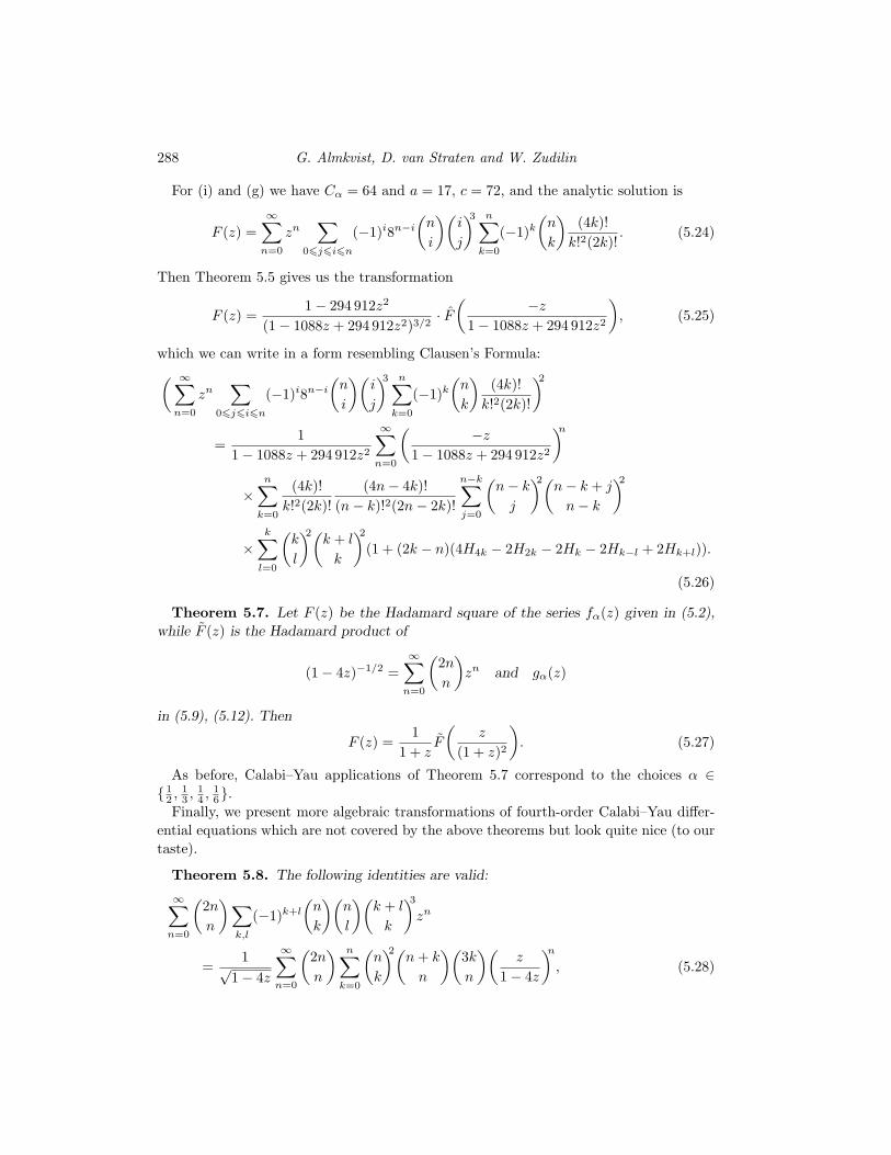
For (i) and (g) we have Cα = 64 and a = 17, c = 72, and the analytic solution is

F (z) =∞∑

n=0

zn∑

0�j�i�n

(−1)i8n−i

(n

i

)(i

j

)3 n∑k=0

(−1)k

(n

k

)(4k)!

k!2(2k)!. (5.24)

Then Theorem 5.5 gives us the transformation

F (z) =1 − 294 912z2

(1 − 1088z + 294 912z2)3/2 · F

(−z

1 − 1088z + 294 912z2

), (5.25)

which we can write in a form resembling Clausen’s Formula:( ∞∑n=0

zn∑

0�j�i�n

(−1)i8n−i

(n

i

)(i

j

)3 n∑k=0

(−1)k

(n

k

)(4k)!

k!2(2k)!

)2

=1

1 − 1088z + 294 912z2

∞∑n=0

(−z

1 − 1088z + 294 912z2

)n

×n∑

k=0

(4k)!k!2(2k)!

(4n − 4k)!(n − k)!2(2n − 2k)!

n−k∑j=0

(n − k

j

)2(n − k + j

n − k

)2

×k∑

l=0

(k

l

)2(k + l

k

)2

(1 + (2k − n)(4H4k − 2H2k − 2Hk − 2Hk−l + 2Hk+l)).

(5.26)

Theorem 5.7. Let F (z) be the Hadamard square of the series fα(z) given in (5.2),while F (z) is the Hadamard product of

(1 − 4z)−1/2 =∞∑

n=0

(2n

n

)zn and gα(z)

in (5.9), (5.12). Then

F (z) =1

1 + zF

(z

(1 + z)2

). (5.27)

As before, Calabi–Yau applications of Theorem 5.7 correspond to the choices α ∈{ 1

2 , 13 , 1

4 , 16}.

Finally, we present more algebraic transformations of fourth-order Calabi–Yau differ-ential equations which are not covered by the above theorems but look quite nice (to ourtaste).

Theorem 5.8. The following identities are valid:

∞∑n=0

(2n

n

) ∑k,l

(−1)k+l

(n

k

)(n

l

)(k + l

k

)3

zn

=1√

1 − 4z

∞∑n=0

(2n

n

) n∑k=0

(n

k

)2(n + k

n

)(3k

n

)(z

1 − 4z

)n

, (5.28)


∞∑n=0

(2n

n

) n∑k=0

(n

k

)2(2k

k

)(2n − 2k

n − k

)zn

=1√

1 − 32z

∞∑n=0

(2n

n

) ∑k,l

(−1)n−k23(n−k)(

n

k

)(k

l

)2(2l

l

)(2k − 2l

k − l

)(z

1 − 32z

)n

,

(5.29)

∞∑n=0

(2n

n

) ∑k,l

(n

k

)(n

l

)(k

l

)(k + l

k

)(2l

l

)(2k

k − l

)zn

=1√

1 − 4z

∞∑n=0

(2n

n

)2 n∑k=0

(n

k

)2(2k

k

)(z

1 − 4z

)n

, (5.30)

∞∑n=0

( n∑k=0

(n

k

)2(n + k

n

))2

zn

=1

1 + z

∞∑n=0

(2n

n

) ∑k,l

(n

k

)(n

l

)(k + l

k

)(2l

l

)(l

k − l

)(z

(1 + z)2

)n

, (5.31)

∞∑n=0

( n∑k=0

(n

k

)(2k

k

)(2n − 2k

n − k

))2

zn

=1

1 − 32z

∞∑n=0

(2n

n

) [n/2]∑k=0

2n−2k

(n

k

)(n − k

k

)(2k

k

)(2n − 2k

n − k

)(z

(1 − 32z)2

)n

,

(5.32)

∞∑n=0

( [n/3]∑k=0

(−1)k3n−3k

(n

3k

)(3k)!k!3

)2

zn

=1

1 − 27z

∞∑n=0

[n/3]∑k=0

(−1)n−k

((2n − 3k − 1

n

)+

(2n − 3k

n

))

× (3k)!k!3

(3n − 3k)!(n − k)!3

(z

(1 − 27z)2

)n

. (5.33)

6. The invariance of Yukawa couplings

As we have already seen, algebraic transformations transform Calabi–Yau equations intosimilar ones, but sometimes look quite different. Such transformations, however, preserve(in a certain precise sense, which we describe below) the Yukawa coupling of the corre-sponding differential equations. Recall that the Yukawa coupling K can be defined, up toa normalization constant factor, through the quotient t(z) = y1(z)/y0(z) ∈ log z + zQ[[z]]of the two solutions y0(z) ∈ 1 + zZ[[z]] and y1(z) of a Calabi–Yau equation (3.3) (see § 2)


as

K =1

y20 · (dt/dz)3

exp(

−12

∫ z

P (z) dz

), (6.1)

and this function is often viewed as a function of q = et, since its q-expansion in thecase of a degenerating family of Calabi–Yau 3-folds is supposed to encode the countingof rational curves of various degrees on a mirror manifold.

On the other hand, we did find several examples of Calabi–Yau equations whoseYukawa couplings coincide, although it is not obvious that the equations themselvesare indeed equivalent in the sense that they are related by an algebraic transformation.At the time of writing, we have discovered and proved algebraic transformations for allpairs of Calabi–Yau equations with equal Yukawa couplings tabulated in [3] (see also thediploma thesis [9]). Most of these transformations (at least those that follow a generalpattern) were given in § 5 and some of them are immediate consequences of the theoremsproven therein. Section 7 describes some of our strategies for finding the transformations.

It is routine to write down the fourth-order linear differential equation

d4Y

dx4 + Pd3Y

dx3 + Qd2Y

dx2 + RdY

dx+ SY = 0 (6.2)

for the function Y (x) = v(x) · y(z(x)). For example, we have

P = −6z′′

z′ + z′P − 4v′

v, (6.3)

where the prime denotes the x-derivative.Clearly, the new equation (6.2) does not necessarily have rational coefficients, but it

does after we impose certain conditions on v(x) and z(x) (for instance, assuming theirrationality). Continuing the computation in (6.3) we obtain the following.

Proposition 6.1 (cf. [12]). Define

Uz(P, Q) = Q − 32

dP

dz− 3

8P 2. (6.4)

ThenUx(P , Q) − (z′)2Uz(P, Q) = 5{z, x}, (6.5)

where

{z, x} =z′′′

z′ − 32

(z′′

z′

)2

(6.6)

is the Schwarzian derivative.

Our next statement shows the invariance of the Yukawa coupling.

Proposition 6.2. Let Y (x) = v(x) · y(z(x)), where z(x) = x + O(x2) and v(x) =1 + O(x). Then the Yukawa couplings defined in accordance with (6.1) coincide:

KY (x) = Ky(z). (6.7)


Proof. Because both the mirror map t(z) and the Yukawa coupling depend on quo-tients of the solutions rather than on the solutions themselves, it is sufficient to treat thecase v(x) = 1. We have the formula (6.1) implying

K =y40

det

(y0 y1

dy0/dz dy1/dz

)3 exp(

−12

∫ z

P (z) dz

)

Furthermore,

dY0

dx= z′ dy0

dz,

dY1

dx= z′ dy1

dzand P = −6

z′′

z′ + z′P ;

hence,

KY (x) =Y 4

0

det

(Y0 Y1

dY0/dx dY1/dx

)3 exp(

−12

∫ x

P (x) dx

)

=y0(z)4

det

(y0(z) y1(z)

z′ dy0/dz z′ dy1/dz

)3 exp(

−12

∫ x (−6

z′′

z′ + z′P (z(x)))

dx

)

=y0(z)4

det

(y0(z) y1(z)

dy0/dz dy1/dz

)3 exp(

−12

∫ z

P (z) dz

)

= Ky(z).

Here we used z′(0) = 1 when we integrated

3∫ x

0

z′′

z′ dx = 3 log z′(x) − 3 log z′(0).

�

From the transformation formulae for passing from (3.3) to (6.2) through the mapY (x) = v(x) · y(z(x)), we find that the Calabi–Yau condition (3.4) is preserved. This isvery hard to see by direct computation, since one gets an enormous fourth-order nonlineardifferential equation for z(x).

Conjecture 6.3. If Yukawa couplings coincide, then there exists an algebraic trans-formation between corresponding Calabi–Yau differential equations.

In fact, Proposition 6.2 states that the Yukawa coupling defined by (6.1) is preserved byany formal coordinate transformation z(x) = x + · · · . However, the requirement for thetransformed equation to be of Calabi–Yau type (in particular, to have rational functionsas coefficients) should lead to the algebraicity of such a transformation.


7. Proof of Theorem 5.4: guessing algebraic transformations

Not only does this section provide a proof of Theorem 5.4 but we also illustrate ourstrategies to guess algebraic transformations for Calabi–Yau differential equations onthe example of Theorem 5.4; more precisely, we show how to ‘discover’ the equivalenceof (e) ∗ (e) and (C) ∗ (i). We distinguish three methods: two analytic and one algebraic.They also provide proofs of the discovered algebraic transformation as soon as the factof its existence is established.

First of all we indicate a way to recognize in Maple whether a function R(z), givenby its Taylor expansion at the origin, is rational or algebraic and, if it is, to find a closedexpression. For this, one applies seriestodiffeq(R, R(z)) (with gfun) and then dsolve

to R(z).

7.1. Analytic guessing

Compute the z-expansions (30 terms, say) of the mirror maps q and q, then write

q(z) = ±q(±z + a2z2 + · · · + a30z

30 + · · · )

(the signs belong together); expand the latter equality up to z31 to get a system of linearequations for unknowns a2, . . . , a30. It takes Maple a few minutes to solve the system;this finds the inner transformation. Then compute the power series expansion of the outertransformation multiple and use gfun.

7.2. Schwarzian relation

In passing from (e) ∗ (e) to (C) ∗ (i), we can use the ‘magic Schwarzian relation’ (Propo-sition 6.1) for z(x) in the form z(x) = −x + · · · . Then we recursively find the expansionfor z(x) = −256z(x/256),

z(x) = x + 10x2 + 83x3 + 628x4 + 4501x5 + 31 134x6 + 210 023x7 + · · · ,

which Maple easily recognizes as the expansion of a rational function

z(x) =x(1 − x)2

(1 − 6x + x2)2.

Furthermore, denoting by Y (z), Y (z) ∈ 1 + zZ[[z]] the analytic solutions of (e) ∗ (e) and(C) ∗ (i), respectively, it remains to let Maple identify the quotient of

Y (z) and Y

(−z(1 − 256z)2

(1 − 6 · 256z + 2562z2)2

)

with the algebraic function (1 − 6 · 256z + 2562z2)−1/2.


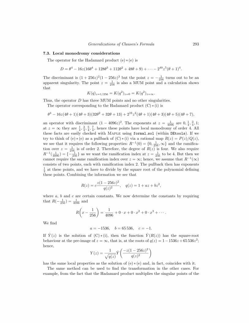
7.3. Local monodromy considerations

The operator for the Hadamard product (e) ∗ (e) is

D = θ4 − 16z(16θ4 + 128θ3 + 112θ2 + 48θ + 9) + · · · − 240z5(θ + 1)4.

The discriminant is (1 + 256z)2(1 − 256z)3 but the point z = − 1256 turns out to be an

apparent singularity. The point z = 1256 is also a MUM point and a calculation shows

thatK(q)z=1/256 = K(q2)z=0 = K(q2)z=∞.

Thus, the operator D has three MUM points and no other singularities.The operator corresponding to the Hadamard product (C) ∗ (i) is

θ4 − 16z(4θ + 1)(4θ + 3)(32θ2 + 32θ + 13) + 216z2(4θ + 1)(4θ + 3)(4θ + 5)(4θ + 7),

an operator with discriminant (1 − 4096z)2. The exponents at z = 14096 are 0, 1

4 , 34 , 1;

at z = ∞ they are 14 , 3

4 , 54 , 7

4 , hence these points have local monodromy of order 4. Allthese facts are easily checked with Maple using formal sol (within DEtools). If wetry to think of (e) ∗ (e) as a pullback of (C) ∗ (i) via a rational map R(z) = P (z)/Q(z),we see that it requires the following properties: R−1(0) = {0, 1

256 ,∞} and the ramifica-tion over z = 1

256 is of order 2. Therefore, the degree of R(z) is four. We also requireR−1( 1

4096 ) = {− 1256} as we want the ramification index at z = 1

256 to be 4. But then wecannot require the same ramification index over z = ∞; hence, we assume that R−1(∞)consists of two points, each with ramification index 2. The pullback then has exponents12 at these points, and we have to divide by the square root of the polynomial definingthese points. Combining the information we see that

R(z) = cz(1 − 256z)2

q(z)2, q(z) = 1 + az + bz2,

where a, b and c are certain constants. We now determine the constants by requiringthat R(− 1

256 ) = 14096 and

R

(x − 1

256

)=

14096

+ 0 · x + 0 · x2 + 0 · x3 + · · · .

We finda = −1536, b = 65 536, c = −1.

If Y (z) is the solution of (C) ∗ (i), then the function Y (R(z)) has the square-rootbehaviour at the pre-image of z = ∞, that is, at the roots of q(z) = 1−1536z +65 536z2;hence,

Y (z) =1√q(z)

Y

(−z(1 − 256z)2

q(z)2

)

has the same local properties as the solution of (e) ∗ (e) and, in fact, coincides with it.The same method can be used to find the transformation in the other cases. For

example, from the fact that the Hadamard product multiplies the singular points of the


operators, it follows without further calculation that the operators (5.20) and (5.21) have0, ∞ and the roots of 1 − 2az + cz2 as singularities. The Hadamard product of fα(z)and operator (2.5) has its singularities at 0, ∞ and the roots of 1 − az + cz2. A possibletransformation of degree 2 will have to map these singular points in exactly the sameway as in Theorem 4.1; hence, we are again led to consider z �→ −z/(1 − az + cz2). Inthis case, the prefactor can also be determined by looking at the local exponents.

8. Concluding remarks

It is definitely not our goal here to stress the consequences of our theorems, since wefeel that the transformations, and even their existence, are beautiful by themselves.Our results provide (albeit rather indirect) geometric interpretations of several (YY-)pullbacks from the table in [3]; previously, such pullbacks were of geometric origin onlyconjecturally, and no relation to Calabi–Yau geometry was known. Another applicationof our transformation theorems, having a more arithmetic flavour, is the integrality ofthe analytic solutions of the pullbacks (condition (ii) of § 2), as well as the integrality ofthe corresponding mirror maps (condition (iii)) when the results in [11] are applicable.There are many aspects that can be discussed elsewhere.

Acknowledgements. The work of G.A. and W.Z. was supported by the Max PlanckInstitute for Mathematics (Bonn). W.Z. acknowledges support by the Hausdorff Centerfor Mathematics (Bonn). We thank Fernando Rodrıguez Villegas and Don Zagier forpointing out the way to make our Theorem 5.5 as general as it is now. Special thanks goto Michael Bogner and Stefan Reiter for many useful remarks and their discovery of the‘strange’ Calabi–Yau differential equation corresponding to (2.7). Finally, we thank thereferee for many helpful suggestions.

The foundations of this work were established during a visit of W.Z. to the Instituteof Algebraic Meditation at Hoor, Sweden (May 26–June 3, 2007). He thanks the staff ofthe institute for their hospitality.

References

1. G. Almkvist, Calabi–Yau differential equations of degree 2 and 3 and Yifan Yang’spullback, Preprint (http://arxiv.org/abs/math.AG/0612215; 2006).

2. G. Almkvist and W. Zudilin, Differential equations, mirror maps and zeta values, inMirror symmetry V (ed. N. Yui, S.-T. Yau and J. D. Lewis), AMS/IP Studies in AdvancedMathematics, Volume 38, pp. 481–515 (American Mathematical Society and InternationalPress, Providence, RI, 2006).

3. G. Almkvist, C. van Enckevort, D. van Straten and W. Zudilin, Tables of Calabi–Yau equations, Preprint (http://arxiv.org/abs/math.AG/0507430; 2005).

4. Y. Andre, G-functions and geometry, Aspects of Mathematics, Volume 13 (Vieweg &Sohn, Braunschweig, 1989).

5. R. Apery, Irrationalite de ζ(2) et ζ(3), in Journees arithmetiques de Luminy, Asterisque,Volume 61, pp. 11–13 (Societe Mathematique de France, Paris, 1979).

6. A. Beauville, Les familles stables de courbes elliptiques sur P1 admettant quatre fibres

singulieres, C. R. Acad. Sci. Paris Ser. I 294 (1982), 657–660.


7. F. Beukers, Irrationality of π2, periods of an elliptic curve and Γ1(5), in Diophantineapproximations and transcendental numbers, Progress in Mathematics, Volume 31, pp. 47–66 (Birkhauser, 1983).

8. F. Beukers, On Dwork’s accessory parameter problem, Math. Z. 241 (2002), 425–444.9. M. Bogner, Differentielle Galoisgruppen und Transformationstheorie fur Calabi-Yau-Op-

eratoren vierter Ordnung, Diploma-Thesis, Institut fur Mathematik, Johannes Gutenberg-Universitat, Mainz (2008).

10. V. V. Golyshev, Classification problems and mirror duality, in Surveys in geometryand number theory: reports on contemporary Russian mathematics, London MathematicalSociety Lecture Note Series, Volume 338, pp. 88–121 (Cambridge University Press, 2007).

11. C. Krattenthaler and T. Rivoal, Multivariate p-adic formal congruences and inte-grality of Taylor coefficients of mirror maps, in Theories galoisiennes et arithmetiques desequations differentielles (ed. L. Di Vizio and T. Rivoal), Seminaires et Congres (SocieteMathematique de France, Paris (in press).

12. B. H. Lian and S.-T. Yau, Differential equations from mirror symmetry, in Surveys indifferential geometry: differential geometry inspired by string theory, Surveys in DifferentialGeometry, Volume 5, pp. 510–526 (International Press, Boston, MA, 1999).

13. R. Miranda and U. Persson, On extremal rational elliptic surfaces, Math. Z. 193(1986), 537–558.

14. C. Peters, Monodromy and Picard–Fuchs equations for families of K3-surfaces andelliptic curves, Annales Sci. Ecole Norm. Sup. (4) 19 (1986), 583–607.

15. C. Peters and J. Stienstra, A pencil of K3-surfaces related to Apery’s recurrence forζ(3) and Fermi surfaces for potential zero, in Arithmetic of complex manifolds, LectureNotes in Mathematics, Volume 1399, pp. 110–127 (Springer, 1989).

16. U. Schmickler-Hirzebruch, Elliptische Flachen uber P1C mit drei Ausnahmefasern

und die hypergeometrische Differentialgleichung, Schriftenreihe des Mathematischen Insti-tuts der Universitat Munster, 2. Serie 33 (Universitat Munster, Mathematisches Institut,Munster, 1985).

17. L. J. Slater, Generalized hypergeometric functions (Cambridge University Press, 1966).18. C. van Enckevort and D. van Straten, Monodromy calculations of fourth-order

equations of Calabi–Yau type, in Mirror symmetry V (ed. N. Yui, S.-T. Yau and J. D.Lewis), AMS/IP Studies in Advanced Mathematics, Volume 38, pp. 539–559 (AmericanMathematical Society and International Press, Providence, RI, 2006).

19. E. T. Whittaker and G. N. Watson, A course of modern analysis, 4th edn (CambridgeUniversity Press, 1927).

20. D. Zagier, Integral solutions of Apery-like recurrence equations, in Groups and symme-tries: from Neolithic Scots to John McKay, CRM Proceedings and Lecture Notes, Vol-ume 47, pp. 349–366 (American Mathematical Society, Providence, RI, 2009).

21. W. Zudilin, Quadratic transformations and Guillera’s formulas for 1/π2, Math. Notes81 (2007), 297–301.

GENERALIZATIONS OF CLAUSEN’S FORMULA AND ALGEBRAIC TRANSFORMATIONS OF ... · Proceedings of the...

Documents

Transcript of GENERALIZATIONS OF CLAUSEN’S FORMULA AND ALGEBRAIC TRANSFORMATIONS OF ... · Proceedings of the...