Generalization of the Generalized Composite Commodity...
35
Generalization of the Generalized Composite Commodity Theorem : Extension based on the Theil’s Aggregation Theory PRELIMINARY- PLEASE DO NOT CITE, QUOTE, OR DISTRIBUTE Dae-Heum Kwon North Dakota State University E-mail: [email protected] David A Bessler Texas A&M University E-mail: [email protected] Selected Paper prepared for presentation at the Agricultural & Applied Economics Association 2009 AAEA & ACCI Joint Annual Meeting, Milwaukee, Wisconsin, July 26-29, 2009. Copyright 2009 by Dae-Heum Kwon and David A Bessler. All rights reserved. Readers may make verbatim copies of this document for non-commercial purposes by any means, provided that this copyright notice appears on all such copies.
Transcript of Generalization of the Generalized Composite Commodity...
Generalization of the Generalized Composite Commodity Theorem
: Extension based on the Theil’s Aggregation Theory
PRELIMINARY- PLEASE DO NOT CITE, QUOTE, OR DISTRIBUTE
Dae-Heum Kwon
North Dakota State University
E-mail: [email protected]
David A Bessler
Texas A&M University
E-mail: [email protected]
Selected Paper prepared for presentation at the Agricultural & Applied Economics Association
2009 AAEA & ACCI Joint Annual Meeting, Milwaukee, Wisconsin, July 26-29, 2009.
Copyright 2009 by Dae-Heum Kwon and David A Bessler. All rights reserved. Readers
may make verbatim copies of this document for non-commercial purposes by any means,
provided that this copyright notice appears on all such copies.

1
1
Generalization of the Generalized Composite Commodity Theorem
: Extension based on the Theil’s Aggregation Theory
Introduction
Empirical studies in economics have relied on various forms of classification and aggregation,
since econometric considerations, such as degrees-of-freedom and multicollinearity, require an
economy of parameters in empirical models. Even though the specific choice of such issues have
been oftentimes based on convenience for addressing specific research objectives rather than on
the empirical evidence for consistent classification and/or aggregation (Shumway and Davis,
2001), it has been demonstrated that small departures from valid classification and/or
aggregation can result in large mistakes in elasticity/flexibility and welfare estimates (Lewbel,
1996). However, identifying a legitimate but less restrictive condition for a consistent
classification and/or aggregation remains an open issue in general.
In the literature of the commodity-wise aggregation, the Hicks-Leontief composite
commodity theorem (Hicks 1936, Leontief 1936) and the homothetic or weak separability
concepts (Leontief 1947) have been proposed. However, it has been demonstrated that these two
types of conditions provide only restrictive possibilities for consistent aggregation in empirical
applications; the empirical tests of both conditions are rejected in most cases. To address such
difficulties, Lewbel (1996) proposed the generalized composite commodity theorem for the
direct demand system in log-linear form. The objective of this study is to further generalize the
Lewbel‟s composite commodity condition based on the Theil‟s aggregation theory (Theil 1954
and 1971).
2
2
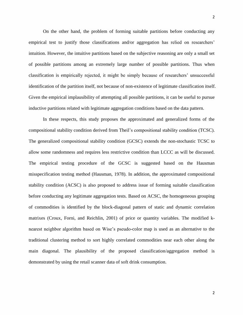
On the other hand, the problem of forming suitable partitions before conducting any
empirical test to justify those classifications and/or aggregation has relied on researchers‟
intuition. However, the intuitive partitions based on the subjective reasoning are only a small set
of possible partitions among an extremely large number of possible partitions. Thus when
classification is empirically rejected, it might be simply because of researchers‟ unsuccessful
identification of the partition itself, not because of non-existence of legitimate classification itself.
Given the empirical implausibility of attempting all possible partitions, it can be useful to pursue
inductive partitions related with legitimate aggregation conditions based on the data pattern.
In these respects, this study proposes the approximated and generalized forms of the
compositional stability condition derived from Theil‟s compositional stability condition (TCSC).
The generalized compositional stability condition (GCSC) extends the non-stochastic TCSC to
allow some randomness and requires less restrictive condition than LCCC as will be discussed.
The empirical testing procedure of the GCSC is suggested based on the Hausman
misspecification testing method (Hausman, 1978). In addition, the approximated compositional
stability condition (ACSC) is also proposed to address issue of forming suitable classification
before conducting any legitimate aggregation tests. Based on ACSC, the homogeneous grouping
of commodities is identified by the block-diagonal pattern of static and dynamic correlation
matrixes (Croux, Forni, and Reichlin, 2001) of price or quantity variables. The modified k-
nearest neighbor algorithm based on Wise‟s pseudo-color map is used as an alternative to the
traditional clustering method to sort highly correlated commodities near each other along the
main diagonal. The plausibility of the proposed classification/aggregation method is
demonstrated by using the retail scanner data of soft drink consumption.

3
3
I. Framework: Theil’s Aggregation theory
Theil‟s aggregation theory is concerned with the transformation of individual relations (micro-
relations) to a relation for the group as a whole (macro-relations) (Theil, 1971). It considers the
possibility that micro-relations can be studied through the macro-relations, where micro-
variables are grouped and represented by macro-variables. The main issue is to understand the
general relationship between micro-parameters and macro-parameters. The ultimate goal is to
identify conditions for the meaningful aggregation that makes it possible to represent micro-
relations by macro-relations.
Theil‟s aggregation theory can be summarized as follows. For a given T time period,
each individual unit has its own linear behavioral relationship. That is, for each individual micro-
unit ( Nn ,.....,1 ), an endogenous variable n
y linearly depends on K exogenous variables
],.....,[1 nKnn
xxx with corresponding micro-parameters ]',.....,[1 nKnn
. These relationships
can be represented by following set of micro-equations.
(1) nnnn
uxy , Nn ,.....,1 .
To study the general tendency of phenomena which are common to most of all Nn ,.....,1
individual micro-unit behaviors, it is postulated that the relation between the aggregated
dependent variable Y and aggregated predetermined variables ],.....,[1 K
XXX can be
represented in the same linear form of micro-equations as the following macro-equation (2).
(2) UXY where
N
n
nyY
1
and
N
n
nxX
1
.
The main issue is the properties of the macro-parameters ]',.....,[1 K
estimated by the
least-squares (LS) estimator, especially in the context of the relationship between macro- and
micro-parameters. To focus on such main issue, the following assumptions are introduced.
4
4
Assumption 0. The N elements of the disturbance vector ntn uu are distributed independently
of micro-regressors ],.....,[1 nKnn
xxx and have zero means.
Assumption 1. The micro-regressors n
x are linearly related with macro-regressors X as
nnnvAXx , where the auxiliary-disturbances
nv are independent of X and have zero means.
The assumption 0 on nnnn
uxy ensures the correctly specified disaggregated model and
implies the independence of nu with macro-regressors X . The assumption 1 on nnn
vAXx
suggests that (i) the LSnn
xXXXA ')'(ˆ 1 is consistent for nA and (ii) nA can be used as the
weighting scheme because )(
1
KK
N
n
nIA
due to
N
n
n
N
n
n
N
n
nn
N
n
nvAXvAXxX
1111
. Note
that the correct specification of the aggregated relation becomes
N
n
n
N
n
nn
N
n
n uxyY
111
and this true aggregated equation has the NK explanatory variables, so it contains as detailed
information as a set of individual micro-relations as a whole, except the loss of information due
to using aggregated dependent variable.
Under these settings, Theil (1954) defines the macro-parameters as mathematical
expectation of its LS estimator and demonstrated following result.
Result 0. If the assumption 0 and 1 hold, the macro-parameters generally depend upon
complicated combinations of corresponding and non-corresponding micro-parameters, i.e.
kE =
N
n
K
kj
njnjka
1
,, =
N
n
K
kj
njnjknk
N
n
nkk aa
1
,,,
1
, , Kk ,.....,1 .
The meaning of the result 0 can be understood more clearly in matrix notation,

5
5
(3)
K
p
ˆ
ˆ
ˆ
lim 2
1
=
N
n
nK
n
n
nKnK
nKn
nKn
nKK
n
n
aa
aa
aa
a
a
a
1
,
,2
,1
,2,1
,2,21
,1,12
,
,22
,11
0
0
0
00
00
00
, where
limp = YXXXp ')'(lim1 , by true aggregation
N
n
n
N
n
nnuxY
11
=
N
n
n
N
n
nn uXXXpxXXXp
1
1
1
1')'(lim')'(lim , by assumption 0 and
nnxXXXA ')'(ˆ 1
=
N
n
nnAp
1
ˆlim =
N
n
nnA
1
, by assumption 1 of nn AAp ˆlim .
Theil‟s conclusion summarized above has negative implications for the aggregate approach. Few
economists will or can meaningfully interpret macro-parameters as complicated mixtures of
heterogeneous components.
However, Theil (1954) identifies two special cases for the possibility of meaningful
aggregation, which are the micro-homogeneity hypothesis and the compositional stability
condition (Pesaran, Pierse, and Kumar 1989) as summarized in results 1 and 2.
Result 1. When the assumption 0 and 1 hold, if each of the micro-parameters has the common
parameters across all individual units (micro-homogeneity), i.e. CNH 21: , then
the macro-parameters capture those common parameters.
(4) CC
N
n
nAp 1
ˆlim , by)(
1
KK
N
n
nIA
under CNH 21: .
Condition 1. (Theil’s compositional stability condition: TCSC), The compositions of each of the
micro-regressors across micro units n
x remain fixed over time with respect to each of the macro-
regressors X , i.e. n
x are non-stochastic linear function of X as (5)
6
6
(5) nn CXx or ],,,[21 nKnn
xxx =
nK
n
n
K
c
c
c
XXX
,
,2
,1
21
00
00
00
],,,[
, Nn ,.....,1 .
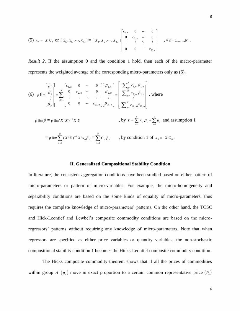
Result 2. If the assumption 0 and the condition 1 hold, then each of the macro-parameter
represents the weighted average of the corresponding micro-parameters only as (6).
(6)
N
nnKnK
N
nnn
N
nnn
N
n
nK
n
n
nK
n
n
K c
c
c
c
c
c
p
,,
,1,2
,1,1
1
,
,2
,1
,
,2
,1
2
1
00
00
00
ˆ
ˆ
ˆ
lim
, where
limp = YXXXp ')'lim(1 , by
N
n
n
N
n
nnuxY
11
and assumption 1
=
N
n
nnxXXXp
1
1')'(lim =
N
n
nnC
1
, by condition 1 of nn CXx .
II. Generalized Compositional Stability Condition
In literature, the consistent aggregation conditions have been studied based on either pattern of
micro-parameters or pattern of micro-variables. For example, the micro-homogeneity and
separability conditions are based on the some kinds of equality of micro-parameters, thus
requires the complete knowledge of micro-parameters‟ patterns. On the other hand, the TCSC
and Hick-Leontief and Lewbel‟s composite commodity conditions are based on the micro-
regressors‟ patterns without requiring any knowledge of micro-parameters. Note that when
regressors are specified as either price variables or quantity variables, the non-stochastic
compositional stability condition 1 becomes the Hicks-Leontief composite commodity condition.
The Hicks composite commodity theorem shows that if all the prices of commodities
within group A A
p move in exact proportion to a certain common representative price A
P
7
7
with fixed vector of constant Aa , i.e. AAA Pap , then (i) an aggregated macro-utility function
defined over composite commodity can be derived from disaggregated micro-utility functions as
AAAABAq
BA PEqaqqUqQUA
|,max, , which has same properties corresponding to
micro-utility functions such as continuity, monotonicity, and quasi-concavity in its arguments;
and (ii) the optimization problem based on disaggregated micro-utility functions as
EqpqpqqU BBAABAqq BA
|,max,
is equivalent to the optimization problem based on aggregated
macro-utility function as EqpQPqQU BBAABAaqQ A
BA
|,max,
in terms of equivalence with
adjustment by constant proportional factor Aa between micro-optimization solution of **,
BAqq
and macro-optimization solution of **,
BAqQ where AAAAA PEqaQ
*** .
While the formal proofs for Hicks composite commodity theorem in the consumer
context and its application in the producer context can be found in Diewert (1978), this result of
Hicks composite commodity theorem can be intuitively understood based on the relationship of
AAAAAAAAAAA QPEqaPqPaqp . Similarly the Leontief-composite commodity
theorem can also be understood by starting with quantity-proportionality AAA Qaq 1 instead of
price-proportionality AAA Pap and the intuitive relationship of AAAAA QPEqp through
AAAAAAAAAA QPQpaQapqp 11 . The problem of Hicks-Leontief composite
commodity condition is that the empirical test are always rejected because the variations in the
price vector within group is restricted by the non-stochastic relation of nkkknk aXx , . Thus the
ratios of the prices (quantities) of individual commodities to composite commodity price
(quantity) are strictly equal to constant proportional factors and remain fixed over time.
From approach of the micro-parameter patterns, it is argued that there can be group
demand functions, when a structural property of preference (or technology) reveals a pattern

8
8
such that the marginal rate of substitution of all pairs of items within the subset is homogenous
of degree zero in the quantities of items within the subset and is also independent of the
quantities of all items outside the subset. While both conditions are required for homothetic
separability, the latter condition is required for weak separability. Although the weakly separable
condition implies only quantity aggregates not price aggregates, both of which are required for
conducting consistent two-stage budgeting (Shumway and Davis, 2001). Although this
separability assumption is less restrictive than the micro-homogeneity assumption, it still implies
rather strong condition as (Lewbel, 1996) pinpoints that “even weak forms of separability impose
very strong elasticity equality restrictions among every good in every group (pp. 525).”
Furthermore, the separability assumption is difficult to test powerfully, and requires
group price indexes that depend on the parameters of the individual utility function (Lewbel,
1996). The empirical issue is that even when enough degrees of freedom are available to estimate
disaggregated models, the multicollinearity among the prices as well as the relatively
complicated cross equation parameter restrictions causes the resulting tests to have little or no
power. In a Monte Carlo study, Barnett and Choi (1989) find that all of the standard tests fail to
reject separability much of the time, even with data constructed from utility functions that are far
from separable. Even though this “difficulty to reject” may be one reason why separability is so
commonly assumed in practice, separability is often empirically rejected (Diewert and Wales,
1995).
In more general setting than commodity aggregation, Zellner (1962) propose hypothesis
test of the micro-homogeneity (4) by the coefficient equality test across micro-units in
disaggregated equations based on the seemingly unrelated regression Equation (SURE) method.
However, Pesaran, Pierse, and Kumar (1989) and Lee, Pesaran, and Pierse (1990) criticize the

9
9
restrictiveness of the micro-homogeneity H as a method of testing aggregation bias and
propose more direct approach based on the following result:
Result 3. The macro-disturbance vector U becomes only the sum of micro-disturbance
N
nnu
1
if the perfect aggregation condition 0:1
XxH
N
nnn is satisfied.
The hypothesis of H has three implications. First, it is demonstrated that the gain in
terms of fitting the macro-dependent variable is not expected by using disaggregated model
rather than aggregated model (Pesaran, Pierse, and Kumar 1989). Second, Lee, Pesaran, and
Pierse (1990) show that the perfect aggregation condition H can hold if 0 nn CXx even
though micro-homogeneity hypothesis is rejected, when the pseudo true macro-parameter value
can be defined by the weighted average of micro-parameters as
N
nnknkkk cp
1,,
ˆlim
because 0:11
N
nnnn
N
nnn CXxXxH . And third implication is that the least
square estimates of macro-parameters are not inconsistent since the macro-disturbance
N
nn
N
nnnn uXuxXYU
11 becomes independent of macro-regressors X by
the assumption 0. Otherwise, consistency is not guaranteed due to the dependency of macro-
regressors X on non-zero components of
N
nnnn CXx
1 .
In this study, we argue that when the pseudo true macro-parameter values are defined by
the weighted average of micro-parameters as
N
nnknkkk cp
1,,
ˆlim , the least square
estimator of macro-parameter is consistent for those pseudo true values under weak condition
without information of micro-parameters by following hypothesis 1 and result 4.
Hypothesis 1. When the micro-regressors n
x are stochastic function of macro-regressors X as
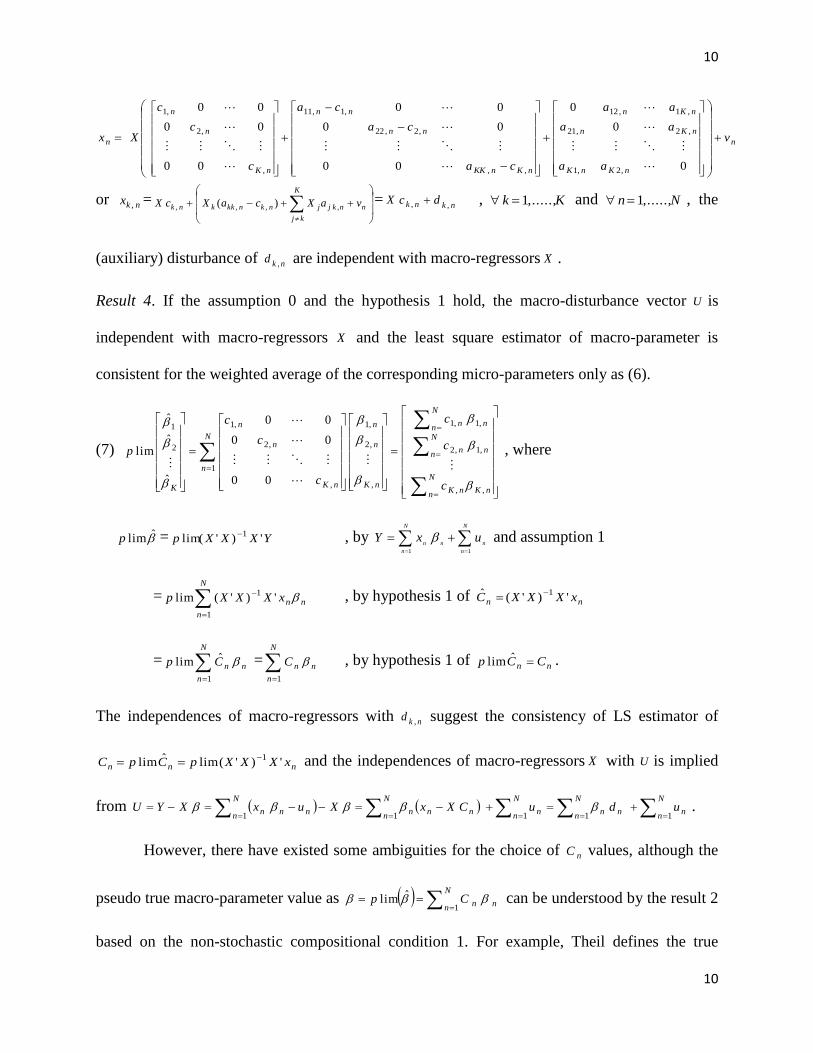
10
10
n
nKnK
nKn
nKn
nKnKK
nn
nn
nK
n
n
n v
aa
aa
aa
ca
ca
ca
c
c
c
Xx
0
0
0
00
00
00
00
00
00
,2,1
,2,21
,1,12
,,
,2,22
,1,11
,
,2
,1
or nkx , =
n
K
kj
nkjjnknkkknk vaXcaXcX ,,,, )( = nknk dcX,, , Kk ,.....,1 and Nn ,.....,1 , the
(auxiliary) disturbance of nkd
, are independent with macro-regressors X .
Result 4. If the assumption 0 and the hypothesis 1 hold, the macro-disturbance vector U is
independent with macro-regressors X and the least square estimator of macro-parameter is
consistent for the weighted average of the corresponding micro-parameters only as (6).
(7)
N
nnKnK
N
nnn
N
nnn
N
n
nK
n
n
nK
n
n
K c
c
c
c
c
c
p
,,
,1,2
,1,1
1
,
,2
,1
,
,2
,1
2
1
00
00
00
ˆ
ˆ
ˆ
lim
, where
limp = YXXXp ')'lim(1 , by
N
n
n
N
n
nnuxY
11
and assumption 1
=
N
n
nnxXXXp
1
1')'(lim
, by hypothesis 1 of nn xXXXC ')'(ˆ 1
=
N
n
nnCp
1
ˆlim =
N
n
nnC
1
, by hypothesis 1 of nn CCp ˆlim .
The independences of macro-regressors with nkd
, suggest the consistency of LS estimator of
nnn xXXXpCpC ')'(limˆlim1
and the independences of macro-regressors X with U is implied
from
N
nn
N
nnn
N
nn
N
nnnn
N
nnnn uduCXxXuxXYU
11111 .
However, there have existed some ambiguities for the choice of nC values, although the
pseudo true macro-parameter value as
N
nnnCp
1
ˆlim can be understood by the result 2
based on the non-stochastic compositional condition 1. For example, Theil defines the true
11
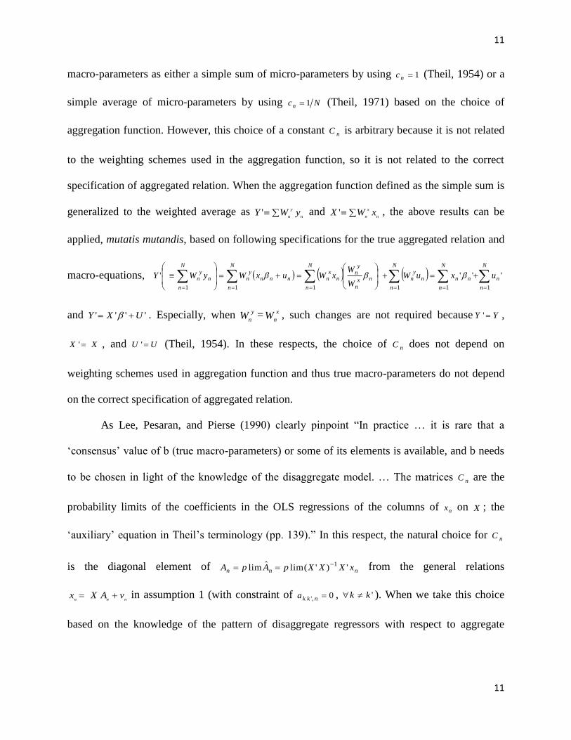
11
macro-parameters as either a simple sum of micro-parameters by using 1nc (Theil, 1954) or a
simple average of micro-parameters by using Ncn 1 (Theil, 1971) based on the choice of
aggregation function. However, this choice of a constant nC is arbitrary because it is not related
to the weighting schemes used in the aggregation function, so it is not related to the correct
specification of aggregated relation. When the aggregation function defined as the simple sum is
generalized to the weighted average as n
y
nyWY ' and n
x
nxWX ' , the above results can be
applied, mutatis mutandis, based on following specifications for the true aggregated relation and
macro-equations,
N
n
N
n
nnn
N
n
ny
n
N
n
nxn
yn
nx
n
N
n
nnny
n
N
n
ny
n uxuWW
WxWuxWyWY
1 11111
''''
and '''' UXY . Especially, when y
nW = x
nW , such changes are not required because YY ' ,
XX ' , and UU ' (Theil, 1954). In these respects, the choice of nC does not depend on
weighting schemes used in aggregation function and thus true macro-parameters do not depend
on the correct specification of aggregated relation.
As Lee, Pesaran, and Pierse (1990) clearly pinpoint “In practice … it is rare that a
„consensus‟ value of b (true macro-parameters) or some of its elements is available, and b needs
to be chosen in light of the knowledge of the disaggregate model. … The matrices nC are the
probability limits of the coefficients in the OLS regressions of the columns of nx on X ; the
„auxiliary‟ equation in Theil‟s terminology (pp. 139).” In this respect, the natural choice for nC
is the diagonal element of nnn xXXXpApA ')'(limˆlim1
from the general relations
nnnvAXx in assumption 1 (with constraint of 0,' nkka , 'kk ). When we take this choice
based on the knowledge of the pattern of disaggregate regressors with respect to aggregate

12
12
regressors, the hypothesis 1 become (8) as the generalization of the non-stochastic compositional
stability condition 1.
(8) nnn dHXx or
n
nKnK
nKn
nKn
nKK
n
n
n v
aa
aa
aa
a
a
a
Xx
0
0
0
00
00
00
,2,1
,2,21
,1,12
,
,22
,11
,
where ],,,[],,,[ ,,,2,2,1,1,,2,1 nK
K
kj
njKjn
K
kj
njjn
K
kj
njjnKnn vaXvaXvaXddd
, Nn ,.....,1 .
The hypothesis 1 in terms of (8) allows randomness of variables as long as the stochastic
disturbances of nd are independent with macro-regressors X in the set of equations
nnndHXx . Hausman (1978) shows that this type of condition can be empirically tested by
using a statistical test of 0:0
n
H in IV
nnnnIVHXx , where IV are instrumental
variables such that IV is closely correlated with regressors X (relevance condition of IV ) and
independent of error n
d (validity condition of IV ). Based on this Hausman type misspecification
testing method, we can empirically test the generalized form of the compositional stability
condition for the consistent aggregation (result 4).
Although it is not easy to identify the appropriate instrumental variables in general setting,
the legitimate instrumental variable can be identified in demand analysis based on dual pairs of
price and quantity for expenditure. The total expenditure variable can be used as the instrumental
variable, when n
x are disaggregated micro-variables of price (quantity) of a specific group and
X are corresponding aggregated macro-variables of price (quantity) of a specific group in the
direct (inverse) demand system. First, the relevance condition can holds since the total
expenditure is closely related with the aggregated price and quantity variables as in estimated
macro-demand systems. Second, the validity condition can also hold based on the relationship of
13
13
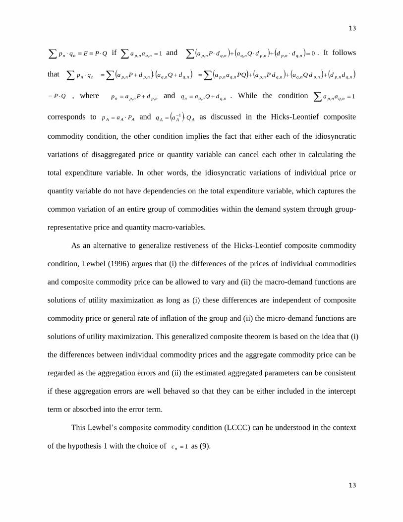
QPEqp nn if 1,, nqnp aa and 0,,,,,, nqnpnpnqnqnp dddQadPa . It follows
that nn qp nqnqnpnp dQadPa ,,,, nqnpnpnqnqnpnqnp dddQadPaPQaa ,,,,,,,,
QP , where npnpn dPap ,, and nqnqn dQaq ,, . While the condition 1,, nqnp aa
corresponds to AAA Pap and AAA Qaq 1 as discussed in the Hicks-Leontief composite
commodity condition, the other condition implies the fact that either each of the idiosyncratic
variations of disaggregated price or quantity variable can cancel each other in calculating the
total expenditure variable. In other words, the idiosyncratic variations of individual price or
quantity variable do not have dependencies on the total expenditure variable, which captures the
common variation of an entire group of commodities within the demand system through group-
representative price and quantity macro-variables.
As an alternative to generalize restiveness of the Hicks-Leontief composite commodity
condition, Lewbel (1996) argues that (i) the differences of the prices of individual commodities
and composite commodity price can be allowed to vary and (ii) the macro-demand functions are
solutions of utility maximization as long as (i) these differences are independent of composite
commodity price or general rate of inflation of the group and (ii) the micro-demand functions are
solutions of utility maximization. This generalized composite theorem is based on the idea that (i)
the differences between individual commodity prices and the aggregate commodity price can be
regarded as the aggregation errors and (ii) the estimated aggregated parameters can be consistent
if these aggregation errors are well behaved so that they can be either included in the intercept
term or absorbed into the error term.
This Lewbel‟s composite commodity condition (LCCC) can be understood in the context
of the hypothesis 1 with the choice of 1nc as (9).

14
14
(9) Lewbelnn dXx or
n
nKKnKnK
nKnn
nKnn
n v
aaa
aaa
aaa
Xx
1
1
1
100
010
001
,,2,1
,2,22,21
,1,12,11
,
where XxvaXaXd nn
K
kj
nkjjnkkkLewbel
nk
,,, )1( , Kk ,.....,1 and Nn ,.....,1 .
The choice of 1nc makes it possible for us to easily define Xxdn
Lewbel
n and allows us to
avoid difficulty involved in searching for instrumental variables in empirically testing the
compositional stability condition. However, it is arbitrary since there is no a prior reason that the
true macro-parameters cannot be a simple average of micro-parameters as discussed.
Furthermore, it is restrictive because it implies that the true macro-parameters should be a simple
sum of micro-parameters. Even if each of the micro-parameters has the common value (micro-
homogeneity), the macro-parameters should be the simple sum of those parameters rather than
those common parameter value itself.
Another ambiguity in Lewbel‟s theorem is how to deal with fact that the Hick-Leontief
composite commodity theorem is based on non-randomness of proportionality factors nkka , ,
given that there are no a priori reasons that the ratio of observed micro-variables to true macro-
variable should be restricted to one. Lewbel deals with this difficulty either (i) by restricting his
generalized theorem into log-linear model which should absorb non-random part of
nk
K
kj njkjnkkk
Lewbel
nkvaXaXd
,,,,)1( into an intercept term in macro-parameter vector of or (ii)
by allowing the differences be absorbed into the random error term of macro-equation. If the first
assumption is taken, the macro-model should always have a significant intercept term, which is a
complicated mixture of heterogeneous components and thus is difficult to be meaningfully
interpreted. If the second assumption is taken, the intuitive rationale of a constant or stable

15
15
budget constraint condition within each commodity group for the Hick-Leontief composite
commodity theorem is lost.
Compared with the Lewbel‟s consistent aggregation condition, the generalized form of
the compositional stability condition maintains (i) the non-randomness of proportionality factors
and thus the intuitive rationale of Hick-Leontief composite commodity theorem and (ii) it does
not have a priori restrictions for true macro-parameters such as simple sum or simple average of
micro-parameters. Furthermore, in contrast to the fact that Lewbel‟s condition is based on the
direct demand system in the log-linear form, (i) the GCSC does not impose any restrictions on
the functional forms except linearity in parameters; and (ii) it can be applied to direct, inverse, as
well as mixed demand systems, where direct (inverse) system assume quantity (price) is a
function of price (quantity) and mixed one captures demand system as a function of mixed set of
price and quantities.
III. Approximated Compositional Stability Condition
Under the assumption 0, Theil reaches his generally negative conclusion for aggregation based
on the assumption 1, which makes it possible to relate the macro-parameters to the micro-
parameters. By replacing this primary assumption with the hypothesis 1 in terms of (8), this
article derives the GCSC for the positive possibility of legitimate aggregation. In other respect,
the GCSC also generalize the non-stochastic condition 1 (TCSC) to allow some randomness in
micro-regressors. This condition is, however, involved with the difficult search for instrumental
variables in a Hausman-type misspecification test in the set of equationsnnn
dHXx . When
appropriate instrumental variables are not available, it is also possible to generalize the TCSC
condition into the approximated compositional stability condition (ACSC).
16
16
The non-stochastic requirement of TCSC is that movements of corresponding micro-
variables across disaggregate units have the absolutely synchronous and perfect degree of co-
movements (the static correlation of one), whereas the non-corresponding micro-regressors are
completely independent. In terms of degree of co-movements, this strict condition can be
approximated by the condition that micro-variables within group are highly correlated but micro-
variables across groups are only weakly correlated over time. This ACSC implies a block-
diagonal pattern of the covariance or correlation matrix among micro-variables as in (10).
(10)
KKKK
K
K
21
22221
11211
, by the ACSC
KK
00
00
00
22
11
, where kk =
1
1
1
2,1,
2,12,
1,21,
NkNk
Nkk
Nkk
.
The main feature of the ACSC is that the ratios of the aggregated macro-variables to
corresponding micro-variables are “near” stable with constant compositional factors over time
but degree of co-movements in non-corresponding micro-regressors across individual units are
very weak ( ', kk ddCov , 'kk where is a small value). In this sense, the TCSC (or GCSC
of Xd n and 0n
dE ) can be approximated by the condition of ', kk ddCov .
Not only the degree of co-movement, but also the way to measure the co-movement can
be generalized. While the TCSC requires that corresponding micro-variables move absolutely
synchronously, the ACSC can allow the possible lead and lag dependencies among micro-
variables within a group, as long as ', kk ddCov holds. While the standard static correlation
only measures synchronous or contemporaneous co-movements between variables and requires
an independence assumption over time, there are several alternative measurements of

17
17
dependency allowing for possible leads and/or lags in dependency among the time-series data in
a dynamic setting. Two of these are the co-integration and the cross correlation. Co-integration is
designed to measure long-run co-movements, so it can be too restrictive to use for identifying
mid-run or short-run or contemporaneous dependency patterns. The cross-correlation with some
leads and lags can capture mid-run or short-run dependency by varying lead and lag parameters,
but the choice of lead and lag parameters can be somewhat arbitrary.
In this respect, we propose to use the standard static correlation as well as the dynamic
correlation defined in (11) and (12) to measure the high co-movements of micro-variables within
a group and near independences of micro-variables across groups.
(11) yx =
yx
yx
SS
C
for frequency where
(12) yx =
dSdS
dC
yx
yx
for frequency band 21
, where 21
0 ,
where x and y are two zero-mean real stochastic processes, x
S and x
S are the spectral
density functions, and yx
C is the co-spectrum of x and y (Croux, Forni, and Reichlin, 2001).
The dynamic correlation, proposed from the frequency domain approach, has useful properties
such as: (a) The dynamic correlation measures different degrees of co-movement which varies
between -1 and 1 just as standard static correlation. (b) The dynamic correlation over the entire
frequency band is identical to static correlation after suitable pre-filtering and it is also related to
stochastic co-integration. (c) The dynamic correlation can be decomposed by frequency and
frequency band, where the low or high frequency band in spectral domain have implication for
the long-run or short-run in time domain respectively (Croux, Forni, and Reichlin, 2001).
This ASCS can also be used for searching specific homogeneous groups of original
variables to form an initial partitioning. In this case, the index k become micro-variables‟ group

18
18
index that should be empirically identified, instead of an index for pre-determined classes of
exogenous variables. The classification issue is important since the empirical rejection of any
consistent aggregation condition can be simply because of researchers‟ unsuccessful
identification of the classification not because of non-existence of legitimate aggregation. The
issue of forming suitable partitions has relied on conventional classification or results of
separability tests. However, the separability approach has some empirical difficulties as
discussed in previous section. The conventional partitions are formed based on several reference
variables such as animal origin, product quality etc., which hopefully proxy consumers‟
unobservable marginal utility structures. This intuition-based approach has an ambiguous aspect,
since alternative choices of reference variables may result in several different classifications.
In these respects, we propose to use the clustering approach based on the ACSC for
searching for specific homogeneous (commodity) groups. This inductive procedure is based on
the idea that (i) the underlying similarity or homogeneity of a group of variables (prices and/or
quantities) can be identified through their high co-movements in dynamics; and (ii) the
classifications are determined by the ACSC to less likely reject the consistent aggregation
condition of the GCSC. The application of cluster method to aggregation problem in economics
is discussed by Fisher (1996) and Pudney (1981) and Nicol (1991) are examples of such
approach for commodity aggregation based on the standard clustering methods such as
hierarchical algorithm.
On the other hand, choice of algorithm for clustering can be important, given that (i) the
resulting classifications implied cluster method can be not economically meaningful and (ii) the
clustering results can depend on the choice of algorithms. For example, the standard clustering
methods, such as hierarchical algorithm and k-mean algorithm, use the correlation matrix as only
19
19
an initial input of similarity measures and thus it is not easy to keep track of information on
correlation matrix (Xu and Wunsch, 2005). In preliminary study, the hierarchical and k-mean
algorithms return different final clustering results. Furthermore, the classifications implied by
these clustering methods are not consistent with the block-diagonal pattern of (10), when the
results are converted into the correlation matrix form. As an alternative, we choose to use the
modified k-nearest neighbor algorithm based on Wise‟s pseudo-color map code in this study.
The main feature of this algorithm is to reorder the variables in the correlation matrix such that
highly correlated variables are sorted near each other along the main diagonal as (10). As will be
discussed, this approach, based on the same correlation matrix used in preliminary study, returns
an intuitively interpretable reordered final correlation matrix.
IV. Empirical Results
The proposed procedures for demand analyses can be summarized as follows: (i) the degree of
co-movements in prices and/or quantities are measured by static and dynamic correlations; (ii)
the measured co-movements are sorted by the modified k-nearest neighbor algorithm to identify
block-diagonal pattern as (10); and (iii) based on the identified classification by the ACSC, the
consistent aggregation condition of GCSC are tested by Hausman misspecification test method.
In addition, the results of GCSC are compared with those based on LCCC. Note that the
empirical tests are conducted for the direct, inverse, as well as mixed demand system in the
differential form such as Rotterdam, CBS, and NBR demand systems. These differential demand
systems are useful to address the nonstationarity issue, which cause several issues for the
empirical test in LCCC. Furthermore, the Rotterdam functional form commonly exists for all
specifications, including Rotterdam mixed demand system (Moschini and Vissa 1993).
20
20
The plausibility of the proposed classification/aggregation method is demonstrated by
using the retail scanner data of soft drinks sold at Dominick‟s Finer Foods (DFF). The
difficulties to identify legitimate classification and aggregation of soft drinks products are
illustrated in Dhar, Chavas, and Gould (2003). After finding statistical evidence against various
classifications of soft drinks suggested in literature based on the weakly separabiliy conditions,
they argue that the classification/aggregation of soft drinks remains a significant challenge to
investigate. The data set consists of weekly observations on 23 soft drink products with size of
6/12 oz sold at DFF from 09:14:1989 through 09:22:1993 with the sample size 210. All the data
are from the Dominick‟s database, which is publicly available from the University of Chicago
Graduate School of Business (http://www.chicagogsb.edu/). Each soft drink used for this study is
a specific soft drink of 6/12 oz size such as Coca-cola classic, Pepsi-cola cans, Seven-up diet can.
The brand-level categories include Coke, Pepsi, Seven-up, Mountain Dew, Sprite, Rite-Cola, Dr.
Pepper, A&W, Canada Dry, Sunkist, and Lipton Brisk. The size of 6/12 oz is chosen due to the
data availability and identified homogeneity within this size of soft drinks in the preliminary
study.
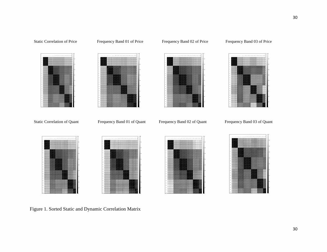
First, to measure co-movement among the disaggregated price and quantity variables,
both the standard static correlation matrix and the dynamic correlation matrix over identified
frequency bands are used. For the dynamic correlation over frequency band, several different
frequency bands are chosen as the non-overlapping bands or regions approximately centered at
peak k
so that jkiijji
0:,, , where the frequency k
is specified
as 2,,1:2 TkTkk
and T is the sample size (Rodrigues, 1999). Note that if the
frequency of a cycle is , the period of the cycle is 2 . Thus, a frequency of Tkk
2
corresponds to a period of kTk2 . We choose common frequency bands to measure co-
21
21
movement among variables with possible leads and lags, based on the estimated spectrums of
variables, which capture dynamics of variables in terms of their cyclic properties with long or
short run trends (Hamilton, 1994). Although there are some degrees of differences, the common
frequency bands can be identified across price and quantity variables and thus among 23
commodities. We use three frequency bands: 0-62, 63-90, and 90-104.5 in terms of k . These
correspond to a period more than 3.37 weeks (frequency Band 01), a period of 3.32 to 2.32
weeks (frequency Band 02), a period of less than 2.30 weeks (frequency Band 03) respectively.
These ranges approximately correspond to 1 month, a half month, and less that a half month
period ranges.
Based on these homogeneity or similarity measure of disaggregate micro-variables, the
modified k-nearest neighbor algorithm is used to sort or reordered the variables such that the
highly correlated variables are near each other along the main diagonal in the reordered
correlation matrix. The final results of the sorted static correlation matrix and dynamic
correlation matrixes for different frequency bands are presented in Figure 1. The black/white
color scheme is used to represent the absolute value of measured correlations, where the darkest
black represents the correlation of 1 and the brightest white represents the correlation of 0. More
detailed information of measured correlation for the standard static correlation coefficient for the
price variables (lower triangular matrix) and quantity variables (upper triangular matrix) is
presented in Table 1. In the static correlation of price and quantity variables, the correlations
among pair of products within the identified group are larger than 0.954 and 0.948 respectively.
Although the correlations of pair-wise variables across different groups show somewhat
different degrees of correlation over the different frequency bands, the common groups of
variables are identified over all the different frequency bands. It is also noticed that both price

22
22
and quantity variables show similar correlation patterns, thus imply the common commodity
classification. Based on these results, the following six groups of soft drink products are
identified as homogeneous groups: (i) Group 1: The Sunkist and Canada Dry product group
(Product of 1 to 4); (ii) Group 2: The Coca-Cola and Sprite product group (Products of 5 to 8);
(iii) Group 3: The Pepsi-Cola and Mountain Dew product group (Product of 9 to 13); (iv) Group
4: The Seven-Up and Dr Pepper product group (Products of 14 to 17); (v) Group 5: The A&W
and Rite-Cola product group (Products of 18 to 21); and (vi) Group 6: The Lipton Brisk product
group (Products of 22 to 23) 1
.
The above classification results can be interpreted as follows: (a) The products of group 2
and 3 correspond to the products of Coca-Cola company (Coca-Cola and Sprite) and Pepsi
company (Pepsi-Cola and Mountain Dew) respectively. (b) The products of group 4 and 5
correspond to the products of competing companies (Seven-Up and Dr Pepper) and following
companies (A&W and Rite-Cola) respectively, given that the Coca-Cola and Pepsi companies
can be interpreted as the market leaders. (c) The products of group 1 and 6 correspond to the
products of different substitutive groups for the carbonate soft drink products. The Sunkist and
Canada Dry brands are identified as a homogenous group, although they represent two different
types of substitute for the carbonate soft drink products. The Lipton Brisk product group shows
different relationships across other groups and thus it is identified distinct group, although this
group is closely related with group 5.
1 The group of 2 and 3 are discriminated by their relatively different relationship with group 5,
given that the variables in group 2 have higher correlation with the variables in group 5. The
group of 3 and 4 are discriminated by their relatively different relationship with group 6, given
that the variables in group 3 have higher correlation with the variables in group 6. The group of 5
and 6 are discriminated by their relatively different relationship with group 3, given that the
variables in group 6 have higher correlation with the variables in group 3.
23
23
The resulting classification can be compared with other standard classifications, which
rely on the conventions for the soft drink products in the literature. For example, one standard
classifications scheme for multi-stage budgeting structures is as follows: (i) All soft drinks are
classified as the branded, private label, and all-other products; (ii) The branded soft drinks are
classified as Cola and Clear sub-segments; and (iii) The Cola sub-segment consists of Coke,
Pepsi, RC Cola and Dr Pepper. On the other hand, the Clear sub-segment consists of Sprite, 7-Up
and Mt. Dew (Dhar, Chavas, and Gould, 2003). Comparing with this and other conventional
classification, the inductive classification of this study has following distinctive features: (a) The
Cola and Clear sub-segments are not identified. (i) Sprite and Mountain Dew brands belong in
their companies‟ brands, Coca-Cola and Pepsi-Cola respectively. (ii) The Seven-Up brand forms
a distinct group with the Dr Pepper brand. (iii) The Rite-Cola brand forms a distinct group with
the A&W brand. (b) The substitutive products for the carbonate soft drink products are classified
as two distinctive groups, where one group consists of Sunkist and Canada Dry brands and the
other group consists of Lipton Brisk product. (c) Diet or caffeine free products do not form
distinctive groups. Note that Dhar, Chavas, and Gould (2003) find that classifications based on
the Cola and Clear sub-segments are empirically rejected. In this respect, it can be argued that
the classification inductively identified in this study provides another plausible classification
scheme for soft drink products.
Then, based on the classification identified by the ACSC, two types of consistent
aggregation conditions (GCSC and LCCC) are empirically tested and compared. Note that both
tests are conducted for both price and quantity variables due to our interest in the alternative
specification among direct, inverse, and mixed demand system. It is worth to emphasize that the
test is actually a joint test for both classification and aggregation. Thus for the robustness check
24
24
of test results, the different index number formulas are used for actual aggregation procedure to
decide weighting schemes for aggregating micro-variables into representative macro-variables
within each identified group. The following different index number formulas are used:
Tornqvist-Theil (dd), Fisher (ff), Paasche (pp), Laspeyres (ll), Fisher with chain (fc), Paasche
with chain (pc), Laspeyres with chain (lc), Unit value (uv), Quantity share weighted index (qw),
and Expenditure share weighted index (ew). The Tornqvist-Theil index is primary used in this
study. The preference toward the Tornqvist-Theil index, especially rather than the Fisher index,
is due to facts that unlike the Fisher index, the Tornqvist-Theil index does not invoke the
problematic assumption of a homothetic or linear homogeneous utility function as discussed in
Hill (2006).
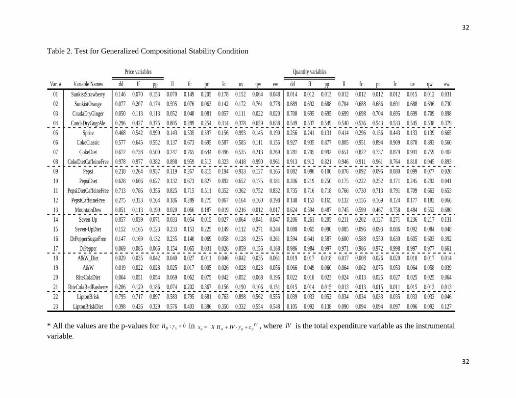
First, the empirical results of the GCSC are presented in Table 2 and can be summarized
as follows, given that a high p-value across almost all test implies a high probability of 0:0
n
H
in IV
nnnnIVHXx , which in turn implies that Xd n in
nnndHXx : (i) The possible
bias due to classification and aggregation for price variable can be ignored and thus the use of
aggregate price variable for representing each group can be justified, when price variables are
used as explanatory variables; (ii) The possible bias due to classification and aggregation for
quantity variable can be ignored and thus the use of aggregate quantity variable for representing
each group can be justified, when quantity variables are used as explanatory variables; and (iii)
The classification itself, which is inductively identified, can be empirically justified in terms of
both price and quantity variables, given that the results are robust with respect to different index
number formulas for aggregation.
In addition, for the comparison with the empirical finding for the Clear soft drink group
in Dhar, Chavas, and Gould (2003), the Sprite, Mt. Dew, 7-up, and 7-up diet are tested as a one
25
25
homogeneous group based on the compositional stability condition. The p-values for 0:0
n
H
are 0.0018 (Sprite), 0.0001 (Mt. Dew), 0.00027 (7-up), and 0.0029 (7-up diet) in terms of the
price variables and 0.000 for all the products in terms of quantity variables, when the Tornqvist-
Theil index is used for price and quantity aggregates. This result is consistent with the empirical
rejection of homogeneity of Sprite, Mt Dew, and 7-up products in Dhar, Chavas, and Gould
(2003) and thus provides additional evidence for the non-existence of the Clear sub-group.
Second, Lewbel‟s generalized compositional commodity condition for differential
demand system is tested based on the correlation test of 0,:0
XdCorrHLewbel
n, where
Xxdn
Lewbel
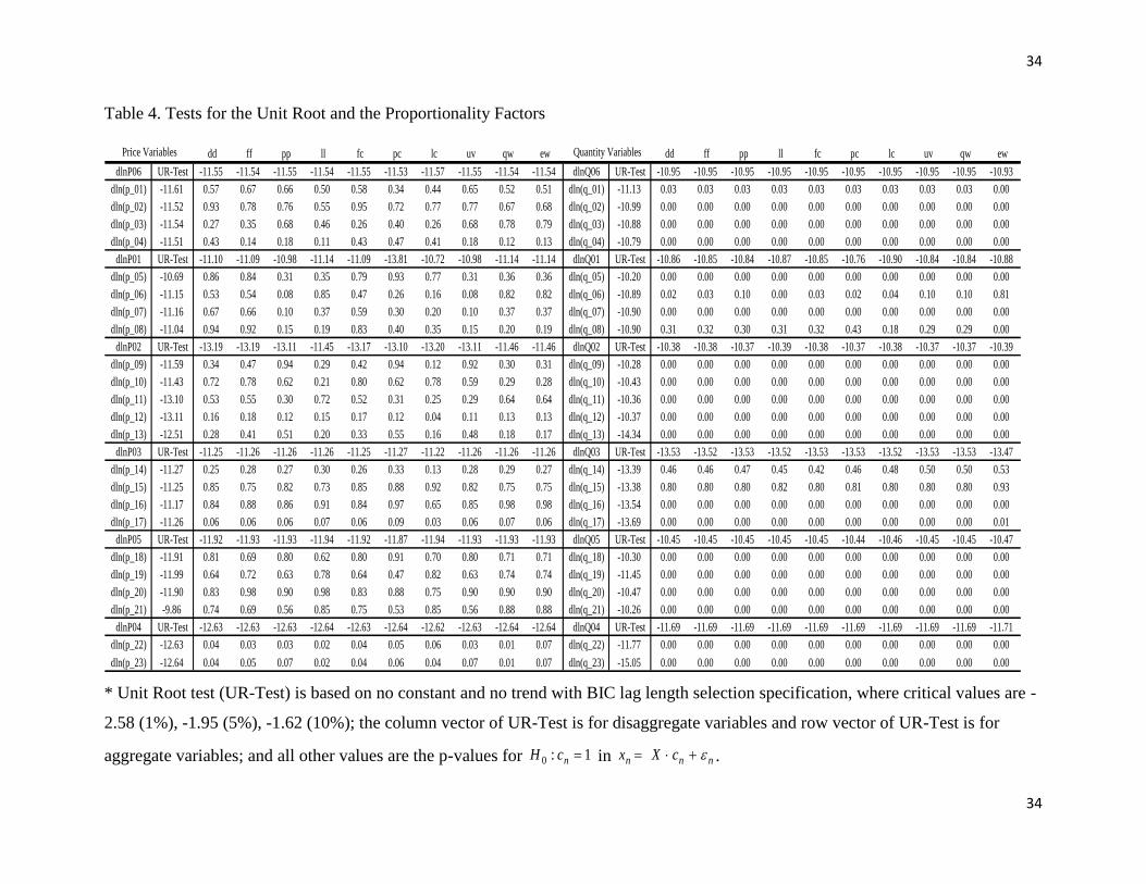
n . The empirical results of the unit root test (UR-test) for micro- and macro-
variables imply stationarity of transformed variables in differential demand system, where unit
root test results for disaggregate variables are in the column vector and those for aggregate
variables are in the row vector under the heads of UR-Test for each group (Table 3.5). These
results of unit root test are robust with respect to other specifications in unit root test. These
results are consistent with the observation in the demand literature that the differential demand
system has been considered as appropriate specification to deal with the possible non-stationarity
problems.
The empirical results of the LCCC are presented in Table 3 and can be summarized as
follows, given that high p-value implies high probability of 0,:0
XdCorrHLewbel
n: (i) The
possible bias due to classification and aggregation for price variable can be ignored and thus the
use of aggregate price variable for representing each group can be justified, when price variables
are used as explanatory variables; (ii) The possible bias due to classification and aggregation for
quantity variable cannot be ignored and thus the use of aggregate quantity variable for
representing each group cannot be justified, when quantity variables are used as explanatory

26
26
variables; and (iii) The test results are ambiguous for classification itself. The classification itself
can be empirically justified in terms of price variables but it cannot be justified in terms of
quantity variables.
The different implications from the two test approaches for quantity variables can be
explained based on the interpretation of the Lewbel‟s condition in the context of Theil‟s
aggregation theory. As discussed, the ambiguity exists in the arbitrary choice on the
proportionality factors 1nc in relationship between micro-variables and macro-variable for
each group. When a high probability of the proportionality factor 1nc is empirically found, the
same test results for the consistent aggregation condition are expected from the two test
approaches. On the other hand, the low p-value of 1:0
n
cH can explain the different results
from the two test approaches. The empirical test results of 1:0
n
cH are presented in Table 3.5.
In general, high p-values are found for price variables, which can explain the same implications
of two test approaches. On the other hand, low p-values are found for quantity variables, which
can explain the different implications of two test approaches.
V. Concluding Remarks
Although the consistent aggregation conditions have been studied based on patterns of either
micro-parameters (e.g. micro-homogeneity and separability hypotheses) or micro-variables (e.g.
compositional stability or composite commodity conditions), identifying a legitimate but less
restrictive conditions remains an open issue. Based on the general aggregation theory, this study
proposes the generalized and approximated compositional stability conditions (GCSC and ACSC)
to address such issue of the consistent classification and aggregation for the demand analyses.
27
27
The proposed procedure does not require restrictions on preferences and information on
micro-parameters and does generalize Hick-Leontief composite commodity condition based on
the pattern of the micro-regressors only. Compared with Lewbel‟s generalized composite
commodity condition (LCCC), our approach does not require a priori restrictions for the true
macro-parameters, maintains the intuitive rationale of Hick-Leontief composite commodity
theorem, and has general application for the direct, inverse as well as mixed demand systems.
The plausibility of the proposed method is demonstrated by using the retail scanner data
of soft drinks consumption. While the application of the ACSC suggests alternative classification
of the soft drinks, the results of the GCSC tests implies the aggregation bias can be ignored in
terms of both price and quantity variables. These results allow the identified classification to be
used for the direct, inverse as well as mixed demand system as aggregated macro-demand
systems, while the results of LCCC restrict the use of that classification for only the direct
demand system. The different implications between ours and Lewbel‟s condition are also
explained by the restrictive condition imposed on the Lewbel‟s composite commodity condition.
28
28
REFERENCES
Barnett, W.A., and S. Choi. 1989. “A Monte Carlo Study of Tests of Blockwise Weak
Separability.” Journal of Business and Economic Statistics 7:363-377.
Croux, C., M. Forni, and L. Reichlin. 2001. “A Measure of Comovements for Economic
Indicators: Theory and Empirics.” The Review of Economics and Statistics 83:232-241.
Dhar, T., J.P. Chavas, and B.W. Gould. 2003. “An Empirical Assessment of Endogeneity Issues
in Demand Analysis for Differentiated Products.” American Journal of Agricultural
Economics 85: 605-617.
Diewert, W.E. 1978. “Superlative Index Numbers and Consistency in Aggregation.”
Econometrica 46:886-900.
Diewert, W.E., and T.J. Wales. 1995. “Flexible Functional Forms and Tests of Homogeneous
Separability.” Journal of Econometrics 67(2):259-302.
Fisher, W.D. 1936. Clustering and Aggregation in Economics. Oxford: Oxford University Press.
Hausman, J.A. 1978. “Specification Tests in Econometrics.” Econometrica 46:1251-1271.
Hicks, J.R. 1936. Value of Capital. Oxford: Oxford University Press.
Hill, R.J. 2006. ”Superlative Index Numbers: Not All of them are Super.” Journal of
Econometrics 130:25-43.
Lee, K.C., M.H. Pesaran, and R.G. Pierse. 1990. “Testing for Aggregation Bias in Linear
Models.” The Economic Journal. 100(400): 137-150.
Leontief, W. 1936. “Composite Commodities and the Problem of Index Numbers.”
Econometrica 4(1): 39-50.
______. 1947. “Introduction to a Theory of the Internal Structure of Functional Relationships.”
Econometrica 15(4): 361-373.

29
29
Lewbel, A. 1996. “Aggregation Without Separability: A Generalized Composite Commodity
Theorem.” American Economic Review 86:524-543.
Moschini, G., and A. Vissa. 1993. “Flexible Specification of Mixed Demand System.” American
Journal of Agricultural Economics 75:1-9.
Nicol, C.J. 1991. “The effects of Expenditure Aggregation on Hypothesis Tests in Consumer
Demand Systems.” International Economic Review. 32(2):405-416.
Pesaran, M.H., R.G. Pierse, and M.S. Kumar. 1989. “Econometric Analysis of Aggregation in
the context of Linear Prediction Models.” Econometrica. 57(4):861-888.
Pudney, S.E. 1981. “An Empirical Method of Approximating the Separable Structure of
Consumer Preferences.” Review of Economic Studies. 48(4):561-577.
Rodrigues, J. 1999. “Classifying Interdependent Time Series in the Frequency Domain.”
ECARES, Universite Libre de Bruxelles, Working Paper.
Shumway, C.R., and G.C. Davis. 2001. “Does Consistent Aggregation really Matter?”
Australian Journal of Agricultural and Resource Economics 45:161-194.
Theil, H. 1954. Linear Aggregation of Economic Relations, Amsterdam: North-Holland.
______ . 1971. Principles of Econometrics. New York: John Wiley & Sons.
Zellner, A. 1962. “An Efficient Method of Estimating Seemingly Unrelated Regressions and
Tests for Aggregation Bias.” Journal of the American Statistical Association.
57(298):348-368.
Xu, R., and D. Wunsch II. May, 2005. “Survey of Clustering Algorithms.” IEEE Transactions on
Neural Networks 16(3):645-678.
30
30
Static Correlation of Price Frequency Band 01 of Price Frequency Band 02 of Price Frequency Band 03 of Price
Static Correlation of Quant Frequency Band 01 of Quant Frequency Band 02 of Quant Frequency Band 03 of Quant
Figure 1. Sorted Static and Dynamic Correlation Matrix
1
2
3
4
5
6
7
8
9
10
11
12
13
14
15
16
17
18
19
20
21
22
23
1 2 3 4 5 6 7 8 9 10
11
12
13
14
15
16
17
18
19
20
21
22
23
-1
-0.9
-0.8
-0.7
-0.6
-0.5
-0.4
-0.3
-0.2
-0.1
0
1
2
3
4
5
6
7
8
9
10
11
12
13
14
15
16
17
18
19
20
21
22
23
1 2 3 4 5 6 7 8 9 10
11
12
13
14
15
16
17
18
19
20
21
22
23
-1
-0.9
-0.8
-0.7
-0.6
-0.5
-0.4
-0.3
-0.2
-0.1
0
1
2
3
4
5
6
7
8
9
10
11
12
13
14
15
16
17
18
19
20
21
22
23
1 2 3 4 5 6 7 8 9 10
11
12
13
14
15
16
17
18
19
20
21
22
23
-1
-0.9
-0.8
-0.7
-0.6
-0.5
-0.4
-0.3
-0.2
-0.1
0
1
2
3
4
5
6
7
8
9
10
11
12
13
14
15
16
17
18
19
20
21
22
23
1 2 3 4 5 6 7 8 9 10
11
12
13
14
15
16
17
18
19
20
21
22
23
-1
-0.9
-0.8
-0.7
-0.6
-0.5
-0.4
-0.3
-0.2
-0.1
0
1
2
3
4
5
6
7
8
9
10
11
12
13
14
15
16
17
18
19
20
21
22
23
1 2 3 4 5 6 7 8 9 10
11
12
13
14
15
16
17
18
19
20
21
22
23
-1
-0.9
-0.8
-0.7
-0.6
-0.5
-0.4
-0.3
-0.2
-0.1
0
1
2
3
4
5
6
7
8
9
10
11
12
13
14
15
16
17
18
19
20
21
22
23
1 2 3 4 5 6 7 8 9 10
11
12
13
14
15
16
17
18
19
20
21
22
23
-1
-0.9
-0.8
-0.7
-0.6
-0.5
-0.4
-0.3
-0.2
-0.1
0
1
2
3
4
5
6
7
8
9
10
11
12
13
14
15
16
17
18
19
20
21
22
23
1 2 3 4 5 6 7 8 9 10
11
12
13
14
15
16
17
18
19
20
21
22
23
-1
-0.9
-0.8
-0.7
-0.6
-0.5
-0.4
-0.3
-0.2
-0.1
0
1
2
3
4
5
6
7
8
9
10
11
12
13
14
15
16
17
18
19
20
21
22
23
1 2 3 4 5 6 7 8 9 10
11
12
13
14
15
16
17
18
19
20
21
22
23
-1
-0.9
-0.8
-0.7
-0.6
-0.5
-0.4
-0.3
-0.2
-0.1
0

31
31
Table 1. Sorted Static Correlation Matrix
Var. # Variable Names dln(01) dln(02) dln(03) dln(04) dln(05) dln(06) dln(07) dln(08) dln(09) dln(10) dln(11) dln(12) dln(13) dln(14) dln(15) dln(16) dln(17) dln(18) dln(19) dln(20) dln(21) dln(22) dln(23)
01 SunkistStrawberry 1.000 0.988 0.983 0.975 0.248 0.272 0.269 0.274 0.282 0.287 0.281 0.289 0.269 0.264 0.282 0.300 0.297 0.212 0.191 0.187 0.189 0.196 0.187
02 SunkistOrange 0.998 1.000 0.988 0.982 0.270 0.297 0.294 0.302 0.308 0.313 0.311 0.316 0.294 0.298 0.317 0.332 0.327 0.237 0.222 0.215 0.210 0.207 0.202
03 CnadaDryGinger 0.998 0.999 1.000 0.994 0.264 0.291 0.287 0.291 0.304 0.310 0.306 0.311 0.293 0.288 0.302 0.317 0.314 0.239 0.223 0.220 0.214 0.218 0.216
04 CandaDryGngrAle 0.998 0.999 1.000 1.000 0.248 0.277 0.275 0.280 0.303 0.310 0.308 0.312 0.294 0.282 0.295 0.311 0.307 0.222 0.206 0.205 0.197 0.202 0.205
05 Sprite 0.279 0.282 0.287 0.291 1.000 0.971 0.968 0.967 0.734 0.740 0.730 0.734 0.728 0.654 0.653 0.637 0.645 0.570 0.568 0.587 0.575 0.537 0.507
06 CokeClassic 0.292 0.295 0.300 0.304 0.955 1.000 0.998 0.995 0.750 0.757 0.746 0.749 0.724 0.671 0.671 0.656 0.662 0.552 0.548 0.569 0.557 0.513 0.483
07 CokeDiet 0.291 0.295 0.300 0.304 0.954 0.999 1.000 0.995 0.748 0.756 0.745 0.748 0.722 0.661 0.661 0.647 0.652 0.550 0.544 0.568 0.555 0.506 0.480
08 CokeDietCaffeineFree 0.293 0.296 0.301 0.305 0.954 0.998 0.999 1.000 0.750 0.758 0.750 0.753 0.724 0.662 0.668 0.657 0.659 0.548 0.543 0.565 0.549 0.509 0.477
09 Pepsi 0.312 0.314 0.319 0.321 0.734 0.756 0.754 0.751 1.000 0.994 0.991 0.989 0.975 0.677 0.683 0.660 0.666 0.453 0.465 0.491 0.461 0.505 0.462
10 PepsiDiet 0.319 0.322 0.326 0.328 0.734 0.755 0.754 0.753 0.998 1.000 0.997 0.996 0.982 0.676 0.679 0.660 0.668 0.458 0.466 0.492 0.467 0.513 0.467
11 PepsiDietCaffeineFree 0.322 0.324 0.329 0.331 0.732 0.753 0.753 0.753 0.995 0.999 1.000 0.997 0.981 0.670 0.674 0.655 0.661 0.449 0.459 0.481 0.454 0.504 0.460
12 PepsiCaffeineFree 0.324 0.326 0.330 0.333 0.732 0.752 0.752 0.752 0.995 0.999 0.999 1.000 0.981 0.675 0.679 0.664 0.671 0.458 0.465 0.484 0.461 0.509 0.458
13 MountainDew 0.325 0.328 0.332 0.334 0.746 0.735 0.735 0.733 0.978 0.981 0.981 0.982 1.000 0.676 0.675 0.656 0.667 0.479 0.492 0.510 0.489 0.536 0.488
14 Seven-Up 0.319 0.321 0.325 0.329 0.652 0.648 0.644 0.642 0.646 0.644 0.641 0.641 0.662 1.000 0.993 0.982 0.988 0.467 0.477 0.490 0.464 0.359 0.316
15 Seven-UpDiet 0.321 0.325 0.329 0.332 0.648 0.645 0.642 0.641 0.643 0.642 0.640 0.641 0.661 0.998 1.000 0.990 0.991 0.458 0.469 0.481 0.449 0.353 0.304
16 DrPepperSugarFree 0.326 0.329 0.333 0.337 0.652 0.644 0.642 0.641 0.638 0.640 0.639 0.641 0.663 0.995 0.996 1.000 0.995 0.453 0.458 0.468 0.439 0.354 0.296
17 DrPepper 0.325 0.328 0.332 0.336 0.659 0.650 0.648 0.646 0.643 0.645 0.644 0.646 0.669 0.995 0.996 0.999 1.000 0.463 0.469 0.476 0.453 0.365 0.304
18 A&W_Diet 0.233 0.238 0.241 0.243 0.592 0.572 0.570 0.568 0.471 0.475 0.473 0.475 0.511 0.558 0.555 0.562 0.564 1.000 0.990 0.977 0.984 0.754 0.712
19 A&W 0.234 0.240 0.242 0.245 0.593 0.574 0.572 0.569 0.472 0.476 0.473 0.476 0.512 0.561 0.557 0.564 0.567 1.000 1.000 0.979 0.979 0.755 0.721
20 RiteColaDiet 0.222 0.228 0.230 0.233 0.601 0.588 0.586 0.584 0.482 0.486 0.483 0.484 0.516 0.541 0.537 0.539 0.544 0.990 0.989 1.000 0.979 0.754 0.722
21 RiteColaRedRasberry 0.224 0.230 0.232 0.235 0.598 0.579 0.578 0.576 0.476 0.479 0.477 0.479 0.515 0.538 0.534 0.540 0.546 0.994 0.994 0.996 1.000 0.750 0.717
22 LiptonBrisk 0.216 0.220 0.224 0.224 0.573 0.546 0.544 0.543 0.556 0.559 0.557 0.560 0.583 0.399 0.395 0.402 0.406 0.747 0.747 0.747 0.750 1.000 0.948
23 LiptonBriskDiet 0.218 0.223 0.226 0.227 0.568 0.541 0.539 0.538 0.547 0.552 0.550 0.553 0.577 0.394 0.391 0.398 0.402 0.748 0.748 0.747 0.751 0.999 1.000
* The lower triangular is for the static correlation coefficients of price variables and the upper triangular is for the static correlation coefficients of quantity
variables and the shaded areas represent the identified groups.
32
32
Table 2. Test for Generalized Compositional Stability Condition
Var. # Variable Names dd ff pp ll fc pc lc uv qw ew dd ff pp ll fc pc lc uv qw ew
01 SunkistStrawberry 0.146 0.070 0.153 0.070 0.149 0.205 0.178 0.152 0.064 0.048 0.014 0.012 0.013 0.012 0.012 0.012 0.012 0.015 0.012 0.031
02 SunkistOrange 0.077 0.207 0.174 0.595 0.076 0.063 0.142 0.172 0.761 0.778 0.689 0.692 0.688 0.704 0.688 0.686 0.691 0.688 0.696 0.730
03 CnadaDryGinger 0.050 0.113 0.113 0.052 0.048 0.081 0.057 0.111 0.022 0.020 0.700 0.695 0.695 0.699 0.698 0.704 0.695 0.699 0.709 0.898
04 CandaDryGngrAle 0.296 0.427 0.375 0.805 0.289 0.254 0.314 0.378 0.659 0.638 0.549 0.537 0.549 0.540 0.536 0.543 0.533 0.545 0.538 0.379
05 Sprite 0.468 0.542 0.990 0.143 0.535 0.597 0.156 0.993 0.145 0.190 0.256 0.241 0.131 0.414 0.296 0.156 0.443 0.133 0.139 0.665
06 CokeClassic 0.577 0.645 0.552 0.137 0.673 0.695 0.587 0.585 0.111 0.155 0.927 0.935 0.877 0.805 0.951 0.894 0.909 0.878 0.893 0.560
07 CokeDiet 0.672 0.738 0.500 0.247 0.765 0.644 0.496 0.535 0.213 0.269 0.781 0.795 0.992 0.651 0.822 0.737 0.879 0.991 0.759 0.402
08 CokeDietCaffeineFree 0.978 0.977 0.382 0.898 0.959 0.513 0.323 0.418 0.990 0.961 0.913 0.912 0.821 0.946 0.911 0.961 0.764 0.818 0.945 0.893
09 Pepsi 0.218 0.264 0.937 0.119 0.267 0.815 0.194 0.933 0.127 0.165 0.082 0.080 0.100 0.076 0.092 0.096 0.080 0.099 0.077 0.020
10 PepsiDiet 0.628 0.606 0.627 0.132 0.673 0.827 0.892 0.652 0.175 0.181 0.206 0.219 0.250 0.175 0.222 0.252 0.171 0.245 0.292 0.041
11 PepsiDietCaffeineFree 0.713 0.786 0.356 0.825 0.715 0.511 0.352 0.362 0.752 0.832 0.735 0.716 0.718 0.766 0.730 0.713 0.791 0.709 0.663 0.653
12 PepsiCaffeineFree 0.275 0.333 0.164 0.186 0.289 0.275 0.067 0.164 0.160 0.198 0.148 0.153 0.165 0.132 0.156 0.169 0.124 0.177 0.183 0.066
13 MountainDew 0.051 0.113 0.190 0.020 0.066 0.187 0.019 0.216 0.012 0.017 0.624 0.594 0.487 0.745 0.599 0.467 0.758 0.484 0.552 0.680
14 Seven-Up 0.057 0.039 0.071 0.033 0.054 0.015 0.027 0.064 0.041 0.047 0.206 0.261 0.205 0.211 0.202 0.127 0.271 0.236 0.217 0.131
15 Seven-UpDiet 0.152 0.165 0.123 0.233 0.153 0.225 0.149 0.112 0.271 0.244 0.088 0.065 0.090 0.085 0.096 0.093 0.086 0.092 0.084 0.048
16 DrPepperSugarFree 0.147 0.169 0.132 0.235 0.140 0.069 0.058 0.128 0.235 0.261 0.594 0.641 0.587 0.600 0.588 0.550 0.630 0.605 0.603 0.392
17 DrPepper 0.069 0.085 0.066 0.154 0.065 0.031 0.026 0.059 0.156 0.168 0.986 0.984 0.997 0.971 0.986 0.972 0.998 0.997 0.977 0.661
18 A&W_Diet 0.029 0.035 0.042 0.040 0.027 0.011 0.046 0.042 0.035 0.061 0.019 0.017 0.018 0.017 0.008 0.026 0.020 0.018 0.017 0.014
19 A&W 0.019 0.022 0.028 0.025 0.017 0.005 0.026 0.028 0.023 0.056 0.066 0.049 0.060 0.064 0.062 0.075 0.053 0.064 0.058 0.039
20 RiteColaDiet 0.064 0.051 0.054 0.069 0.062 0.075 0.042 0.052 0.068 0.196 0.022 0.018 0.023 0.024 0.013 0.025 0.027 0.025 0.025 0.064
21 RiteColaRedRasberry 0.206 0.129 0.186 0.074 0.202 0.367 0.156 0.190 0.106 0.151 0.015 0.014 0.015 0.013 0.013 0.015 0.011 0.015 0.013 0.013
22 LiptonBrisk 0.795 0.717 0.897 0.583 0.795 0.681 0.763 0.898 0.562 0.555 0.039 0.033 0.052 0.034 0.034 0.033 0.035 0.033 0.033 0.046
23 LiptonBriskDiet 0.398 0.426 0.329 0.576 0.403 0.386 0.350 0.332 0.554 0.548 0.105 0.092 0.138 0.090 0.094 0.094 0.097 0.096 0.092 0.127
Quantity variablesPrice variables
* All the values are the p-values for 0:0 nH in IV
nnnn IVHXx , where IV is the total expenditure variable as the instrumental
variable.

33
33
Table 3. Test for Lewbel‟s Composite Commodity Condition
Var. # Variable Names dd ff pp ll fc pc lc uv qw ew dd ff pp ll fc pc lc uv qw ew
01 SunkistStrawberry 0.458 0.559 0.550 0.572 0.457 0.441 0.478 0.550 0.494 0.495 0.197 0.202 0.203 0.202 0.196 0.194 0.199 0.203 0.203 0.019
02 SunkistOrange 0.126 0.087 0.077 0.098 0.126 0.128 0.126 0.077 0.100 0.100 0.000 0.000 0.000 0.000 0.000 0.000 0.000 0.000 0.000 0.000
03 CnadaDryGinger 0.070 0.264 0.269 0.305 0.071 0.094 0.071 0.269 0.200 0.200 0.000 0.000 0.000 0.000 0.000 0.000 0.000 0.000 0.000 0.000
04 CandaDryGngrAle 0.807 0.908 0.900 0.909 0.807 0.796 0.831 0.900 0.963 0.963 0.000 0.000 0.000 0.000 0.000 0.000 0.000 0.000 0.000 0.000
05 Sprite 0.748 0.670 0.209 0.595 0.659 0.483 0.774 0.212 0.614 0.610 0.000 0.000 0.000 0.000 0.000 0.000 0.000 0.000 0.000 0.000
06 CokeClassic 0.854 0.804 0.206 0.547 0.754 0.433 0.378 0.204 0.552 0.551 0.005 0.006 0.036 0.000 0.007 0.014 0.004 0.036 0.036 0.959
07 CokeDiet 0.740 0.699 0.177 0.797 0.654 0.382 0.305 0.176 0.802 0.802 0.000 0.000 0.000 0.000 0.000 0.000 0.000 0.000 0.000 0.000
08 CokeDietCaffeineFree 0.694 0.658 0.175 0.930 0.619 0.368 0.303 0.174 0.934 0.934 0.038 0.038 0.038 0.036 0.038 0.046 0.030 0.038 0.038 0.000
09 Pepsi 0.072 0.094 0.352 0.076 0.090 0.333 0.067 0.370 0.079 0.079 0.000 0.000 0.000 0.000 0.000 0.000 0.000 0.000 0.000 0.000
10 PepsiDiet 0.688 0.659 0.951 0.603 0.706 0.996 0.996 0.920 0.783 0.783 0.000 0.000 0.000 0.000 0.000 0.000 0.000 0.000 0.000 0.001
11 PepsiDietCaffeineFree 0.334 0.391 0.361 0.175 0.366 0.392 0.132 0.344 0.146 0.146 0.000 0.000 0.000 0.000 0.000 0.000 0.000 0.000 0.000 0.000
12 PepsiCaffeineFree 0.127 0.159 0.188 0.044 0.149 0.207 0.037 0.178 0.037 0.037 0.000 0.000 0.000 0.000 0.000 0.000 0.000 0.000 0.000 0.000
13 MountainDew 0.225 0.263 0.367 0.144 0.251 0.394 0.123 0.354 0.133 0.133 0.000 0.000 0.000 0.000 0.000 0.000 0.000 0.000 0.000 0.000
14 Seven-Up 0.112 0.113 0.085 0.150 0.112 0.108 0.122 0.088 0.152 0.152 0.732 0.726 0.739 0.712 0.732 0.733 0.730 0.737 0.737 0.888
15 Seven-UpDiet 0.976 0.966 0.990 0.947 0.976 0.978 0.979 0.998 0.935 0.934 0.727 0.720 0.734 0.706 0.727 0.729 0.725 0.732 0.732 0.578
16 DrPepperSugarFree 0.559 0.543 0.542 0.542 0.559 0.561 0.555 0.536 0.584 0.585 0.000 0.000 0.000 0.000 0.000 0.000 0.000 0.000 0.000 0.001
17 DrPepper 0.066 0.067 0.069 0.065 0.066 0.067 0.065 0.067 0.064 0.064 0.000 0.000 0.000 0.000 0.000 0.000 0.000 0.000 0.000 0.010
18 A&W_Diet 0.972 0.967 0.931 0.968 0.974 0.825 0.904 0.931 0.888 0.889 0.000 0.000 0.000 0.000 0.000 0.000 0.000 0.000 0.000 0.000
19 A&W 0.678 0.660 0.633 0.662 0.680 0.559 0.788 0.633 0.613 0.614 0.000 0.000 0.000 0.000 0.000 0.000 0.000 0.000 0.000 0.000
20 RiteColaDiet 0.725 0.856 0.864 0.888 0.724 0.869 0.632 0.864 0.822 0.823 0.000 0.000 0.000 0.000 0.000 0.000 0.000 0.000 0.000 0.000
21 RiteColaRedRasberry 0.800 0.862 0.988 0.753 0.799 0.944 0.709 0.988 0.743 0.743 0.000 0.000 0.000 0.000 0.000 0.000 0.000 0.000 0.000 0.000
22 LiptonBrisk 0.268 0.204 0.191 0.220 0.269 0.239 0.306 0.191 0.226 0.226 0.000 0.000 0.000 0.000 0.000 0.000 0.000 0.000 0.000 0.000
23 LiptonBriskDiet 0.196 0.243 0.273 0.218 0.196 0.217 0.182 0.273 0.224 0.224 0.000 0.000 0.000 0.000 0.000 0.000 0.000 0.000 0.000 0.000
Price variables Quantity variables
* All the values are the p-values for 0,:0
XdCorrHLewbel
n where Xxd n
Lewbeln .
34
34
Table 4. Tests for the Unit Root and the Proportionality Factors
dd ff pp ll fc pc lc uv qw ew dd ff pp ll fc pc lc uv qw ew
dlnP06 UR-Test -11.55 -11.54 -11.55 -11.54 -11.55 -11.53 -11.57 -11.55 -11.54 -11.54 dlnQ06 UR-Test -10.95 -10.95 -10.95 -10.95 -10.95 -10.95 -10.95 -10.95 -10.95 -10.93
dln(p_01) -11.61 0.57 0.67 0.66 0.50 0.58 0.34 0.44 0.65 0.52 0.51 dln(q_01) -11.13 0.03 0.03 0.03 0.03 0.03 0.03 0.03 0.03 0.03 0.00
dln(p_02) -11.52 0.93 0.78 0.76 0.55 0.95 0.72 0.77 0.77 0.67 0.68 dln(q_02) -10.99 0.00 0.00 0.00 0.00 0.00 0.00 0.00 0.00 0.00 0.00
dln(p_03) -11.54 0.27 0.35 0.68 0.46 0.26 0.40 0.26 0.68 0.78 0.79 dln(q_03) -10.88 0.00 0.00 0.00 0.00 0.00 0.00 0.00 0.00 0.00 0.00
dln(p_04) -11.51 0.43 0.14 0.18 0.11 0.43 0.47 0.41 0.18 0.12 0.13 dln(q_04) -10.79 0.00 0.00 0.00 0.00 0.00 0.00 0.00 0.00 0.00 0.00
dlnP01 UR-Test -11.10 -11.09 -10.98 -11.14 -11.09 -13.81 -10.72 -10.98 -11.14 -11.14 dlnQ01 UR-Test -10.86 -10.85 -10.84 -10.87 -10.85 -10.76 -10.90 -10.84 -10.84 -10.88
dln(p_05) -10.69 0.86 0.84 0.31 0.35 0.79 0.93 0.77 0.31 0.36 0.36 dln(q_05) -10.20 0.00 0.00 0.00 0.00 0.00 0.00 0.00 0.00 0.00 0.00
dln(p_06) -11.15 0.53 0.54 0.08 0.85 0.47 0.26 0.16 0.08 0.82 0.82 dln(q_06) -10.89 0.02 0.03 0.10 0.00 0.03 0.02 0.04 0.10 0.10 0.81
dln(p_07) -11.16 0.67 0.66 0.10 0.37 0.59 0.30 0.20 0.10 0.37 0.37 dln(q_07) -10.90 0.00 0.00 0.00 0.00 0.00 0.00 0.00 0.00 0.00 0.00
dln(p_08) -11.04 0.94 0.92 0.15 0.19 0.83 0.40 0.35 0.15 0.20 0.19 dln(q_08) -10.90 0.31 0.32 0.30 0.31 0.32 0.43 0.18 0.29 0.29 0.00
dlnP02 UR-Test -13.19 -13.19 -13.11 -11.45 -13.17 -13.10 -13.20 -13.11 -11.46 -11.46 dlnQ02 UR-Test -10.38 -10.38 -10.37 -10.39 -10.38 -10.37 -10.38 -10.37 -10.37 -10.39
dln(p_09) -11.59 0.34 0.47 0.94 0.29 0.42 0.94 0.12 0.92 0.30 0.31 dln(q_09) -10.28 0.00 0.00 0.00 0.00 0.00 0.00 0.00 0.00 0.00 0.00
dln(p_10) -11.43 0.72 0.78 0.62 0.21 0.80 0.62 0.78 0.59 0.29 0.28 dln(q_10) -10.43 0.00 0.00 0.00 0.00 0.00 0.00 0.00 0.00 0.00 0.00
dln(p_11) -13.10 0.53 0.55 0.30 0.72 0.52 0.31 0.25 0.29 0.64 0.64 dln(q_11) -10.36 0.00 0.00 0.00 0.00 0.00 0.00 0.00 0.00 0.00 0.00
dln(p_12) -13.11 0.16 0.18 0.12 0.15 0.17 0.12 0.04 0.11 0.13 0.13 dln(q_12) -10.37 0.00 0.00 0.00 0.00 0.00 0.00 0.00 0.00 0.00 0.00
dln(p_13) -12.51 0.28 0.41 0.51 0.20 0.33 0.55 0.16 0.48 0.18 0.17 dln(q_13) -14.34 0.00 0.00 0.00 0.00 0.00 0.00 0.00 0.00 0.00 0.00
dlnP03 UR-Test -11.25 -11.26 -11.26 -11.26 -11.25 -11.27 -11.22 -11.26 -11.26 -11.26 dlnQ03 UR-Test -13.53 -13.52 -13.53 -13.52 -13.53 -13.53 -13.52 -13.53 -13.53 -13.47
dln(p_14) -11.27 0.25 0.28 0.27 0.30 0.26 0.33 0.13 0.28 0.29 0.27 dln(q_14) -13.39 0.46 0.46 0.47 0.45 0.42 0.46 0.48 0.50 0.50 0.53
dln(p_15) -11.25 0.85 0.75 0.82 0.73 0.85 0.88 0.92 0.82 0.75 0.75 dln(q_15) -13.38 0.80 0.80 0.80 0.82 0.80 0.81 0.80 0.80 0.80 0.93
dln(p_16) -11.17 0.84 0.88 0.86 0.91 0.84 0.97 0.65 0.85 0.98 0.98 dln(q_16) -13.54 0.00 0.00 0.00 0.00 0.00 0.00 0.00 0.00 0.00 0.00
dln(p_17) -11.26 0.06 0.06 0.06 0.07 0.06 0.09 0.03 0.06 0.07 0.06 dln(q_17) -13.69 0.00 0.00 0.00 0.00 0.00 0.00 0.00 0.00 0.00 0.01
dlnP05 UR-Test -11.92 -11.93 -11.93 -11.94 -11.92 -11.87 -11.94 -11.93 -11.93 -11.93 dlnQ05 UR-Test -10.45 -10.45 -10.45 -10.45 -10.45 -10.44 -10.46 -10.45 -10.45 -10.47
dln(p_18) -11.91 0.81 0.69 0.80 0.62 0.80 0.91 0.70 0.80 0.71 0.71 dln(q_18) -10.30 0.00 0.00 0.00 0.00 0.00 0.00 0.00 0.00 0.00 0.00
dln(p_19) -11.99 0.64 0.72 0.63 0.78 0.64 0.47 0.82 0.63 0.74 0.74 dln(q_19) -11.45 0.00 0.00 0.00 0.00 0.00 0.00 0.00 0.00 0.00 0.00
dln(p_20) -11.90 0.83 0.98 0.90 0.98 0.83 0.88 0.75 0.90 0.90 0.90 dln(q_20) -10.47 0.00 0.00 0.00 0.00 0.00 0.00 0.00 0.00 0.00 0.00
dln(p_21) -9.86 0.74 0.69 0.56 0.85 0.75 0.53 0.85 0.56 0.88 0.88 dln(q_21) -10.26 0.00 0.00 0.00 0.00 0.00 0.00 0.00 0.00 0.00 0.00
dlnP04 UR-Test -12.63 -12.63 -12.63 -12.64 -12.63 -12.64 -12.62 -12.63 -12.64 -12.64 dlnQ04 UR-Test -11.69 -11.69 -11.69 -11.69 -11.69 -11.69 -11.69 -11.69 -11.69 -11.71
dln(p_22) -12.63 0.04 0.03 0.03 0.02 0.04 0.05 0.06 0.03 0.01 0.07 dln(q_22) -11.77 0.00 0.00 0.00 0.00 0.00 0.00 0.00 0.00 0.00 0.00
dln(p_23) -12.64 0.04 0.05 0.07 0.02 0.04 0.06 0.04 0.07 0.01 0.07 dln(q_23) -15.05 0.00 0.00 0.00 0.00 0.00 0.00 0.00 0.00 0.00 0.00
Price Variables Quantity Variables
* Unit Root test (UR-Test) is based on no constant and no trend with BIC lag length selection specification, where critical values are -
2.58 (1%), -1.95 (5%), -1.62 (10%); the column vector of UR-Test is for disaggregate variables and row vector of UR-Test is for
aggregate variables; and all other values are the p-values for 1:0 ncH in nnn cXx .