Generalising Algorithm Performance

in Instance Space

Kate Smith-Miles and Leo LopesSchool of Mathematical Sciences

Monash University, Melbourne, Australia

Automated Algorithm Selection

• We need to understand when an algorithm can be

expected to perform well

– What are the characteristics or features of the

instances that make this algorithm excel or fail?

– Can we predict, for a given instance, the performance

of an algorithm (or portfolio of algorithms)?

• The same question can be applied to other

decision we have to make

– parameter tuning, branching strategy, etc.

• Tools like Dr. AMPL assist with solver selection

• Lots of techniques we can borrow from AISmith-Miles, K. A., “Cross-disciplinary perspectives on meta-learning

for algorithm selection”, ACM Computing Surveys, vol. 41, no. 1, article 6, 2008.

Automated solver selection

• Statistical or machine learning techniques can be

used to learn from past experimental results

– infer relationships between features of the problem and

the performance of solvers (or parameters etc.)

– Sub-field known as “Intelligent Optimisation”

Hutter, Hoos, Leyton-Brown., “Automated configuration of mixed integer

programming solvers”, Integration of AI and OR Techniques in Constraint

Programming for Combinatorial Optimization Problems, Springer, 2010.

Smith-Miles, K. and van Hemert, J. “Discovering the Suitability of Optimisation

Algorithms by Learning from Evolved Instances”, Annals of Mathematics and

Artificial Intelligence, DOI 10.1007/s10472-011-9230-5, in press.

Smith-Miles, James, Giffin and Tu, “A Knowledge Discovery Approach to

Understanding Relationships between Scheduling Problem Structure and Heuristic

Performance”, in Stutzle, T. (ed.), Selected papers of LION3, 2009.

Beyond automated solver selection

• We don’t just want advice about picking the

winner

• We want insights into the strengths and

weaknesses of different solvers or algorithmic

approaches

– Why do they succeed or fail?

– Under what conditions (problem characteristics) are

they suitable?

– Do these conditions include characteristics of real-

world instances?

– Is this solver only good where others are also good,

or there instances where it is uniquely suited?

No Free Lunch Theorems

• "...for any algorithm, any elevated performance over one

class of problems is exactly paid for in performance over

another class." Wolpert and Macready (1997)

• We need to challenge the standard publishing

practice:

– Show how well your new algorithm performs on a

chosen set of test instances, or standard benchmarks

– This doesn’t reveal the true strengths and weaknesses

• We could demand greater insights if we develop

suitable tools to explore the whole instance space

Wolpert, D. and Macready, W. “No Free Lunch Theorems for Optimization”,

IEEE Transactions on Evolutionary Computation, 1 (1997), 67-82.

Algorithm Footprints

• When claiming a certain algorithm performance it

is important (but rare) to describe the boundaries

of that performance in instance space.

• The “footprint” of an algorithm is defined as the

generalised region in instance space where the

algorithm is expected to perform well.

• “understanding these footprints, how they vary

between algorithms and across instance space

dimensions, may lead to a future platform for

wiser algorithm-choice decisions”

Corne, D., Reynolds, A.: Optimisation and Generalisation: Footprints in Instance

Space. Parallel Problem Solving from Nature PPSN XI (2010) 22-31.

Visualising instance space

• Suppose that suitable features of an instance can be

measured

– E.g. TSP instances could be summarised by

• The number of cities

• Statistical properties of the inter-city distance matrix

– Fraction of distinct distances

– Triangle inequality satisfaction

– Standard deviation of distances

• Cluster structure

– Ratio of clusters to cities; ration of outliers to cities

– Instances that are similar have a similar feature vector

– If we have the right feature set, then the performance of an

algorithm should be similar for instances that are “similar”

(near in n-dimensional feature space)

Smith-Miles, K., Lopes, L.: Measuring Instance Difficulty for Combinatorial

Optimization Problems, Computers and Operations Research, in press.

Footprints, continued

• Corne and Reynolds selected two features at

a time to visualise an instance space, and

show the performance of algorithms

• Higher dimensional features spaces contain

potentially richer information to explain

algorithm performance

• We need visualisation techniques for instance

spaces defined by a large number of

features, and learning methods to define the

boundaries of the algorithm footprint.

Instance generation methods

• What we learn about the footprint of an algorithm

though is determined by the instances we select,

as well as the features we measure

• Typically, instances for testing optimisation

algorithms are either

– real world optimisation problems or

– synthetically generated via some instance generation

procedure.

• However, it is often challenging to synthetically

generate instances that are real-world-like or

discriminating of solver performanceHill, R., Reilly, C.: The effects of coefficient correlation structure in 2-dimensional

knapsack problems on solution procedure performance. Manag. Sci (2000) 302-317

Methodology

• Our case study will show how different types

of instances can be visualised in a high-

dimensional feature space

– Select relevant features

– Define instances by high dimensional feature

vector

– Project instances onto two-dimensional map

– Visually explore location of different types of

instances (real, synthetic)

– Visually explore algorithm footprint

– Learn and report boundary of algorithm footprint

Case study: Timetabling

• Udine Timetabling problem aka Curriculum-

based Course Timetabling (CTT) problem.

• CTT used for track 3 of ITC 2007

• We have chosen this problem as a case study

for three reasons:

– the existence of instance generators as well as real-

world instances;

– access to two of the top five search heuristics from

ITC2007;

– Timetabling is a complex (branch) problem with an

underlying core problem of graph colouring

Thanks to Jakub Mareček, Tomás Müller, and Koji Nonobe,

and their open source contributions

Defining the timetabling problem

• Students follow specific tracks of coursework

that lead to a degree.

• Conflicts occur for both students and teachers if

they have clashes

• The set of all conflicts within an instance of the

CTT is captured by a conflict graph G(V,E)

– V is a set of vertices corresponding to “events” that

need to be timetabled

– E is a set of edges connecting two vertices when

those two events cannot occur at the same time

• Conflict graphs are created for teachers and the

curriculum

Soft constraints

• Penalties are applied for violation of soft

constraints. For example,

– Avoid scheduling different lectures of the

same course in different rooms

– Avoid using large venues for small classes

– Avoid large gaps in a student’s timetable

• We measure the performance of an

algorithm as the number of penalties

after 600 seconds of runtime

Algorithms

• We consider two highly competitive

algorithms provided by ITC 2007

competitors:

– Algorithm A (TSCS) is a Tabu Search over

a weighed constraint satisfaction problem

written in C++.

– Algorithm B (SACP) is a constraint

propagation code combined with Simulated

Annealing written in Java.

Defining the features of instances

1. Graph Colouring features

• From each of: the curriculum conflict graph; the teacher conflict graph; and

the combined conflict graph (both weighted by enrolment, and unweighted)

we calculated:

– The density (connectivity) of the graph.

– Mean and standard deviation of the distribution of node clustering indexes.

– Mean and standard deviation of the event degree distribution

• Estimate of the number of colours needed for graph colouring (based on

DSATUR heuristic)

• Sum of the colour values over all nodes

2. Timetabling features:

• Slack (total seats offered - course requests)

• Mean and standard deviation of the distribution of course enrolments.

• Mean and standard deviation of the distribution of the number of rooms into

which a course may fit.

• Number of events that will only fit in one room.

32 candidate

features in

total

Instances

• We have utilised three sets of instances:

– the original 21 from the competition;

– a set of 4500 obtained using the generator by

Maracek and Burke;

– and another set of 4500 that we have generated to

be similar to real-world instances and

differentiating of algorithm performance

Most instances resulted in tied

outcomes for both algorithms

Lopes, L., Smith-Miles, K.: Generating applicable synthetic instances for branch

problems. Operations Research, under review

Algorithms

{A}

Empirical

Rules

Theoretical

Support

(Meta-)learning

of meta-data

Algorithm Performance

Results {Y}

Dataset Features

{F}

Problem instances

{P}

Automated

Algorithm Selection

Refinement

of Algorithms

1

7 65

43

2

8

PHASE 1

PHASE 2

PHASE 3

The “bigger picture” – design of better algorithms and

knowing when to use them!

Meta-data

• P – set of 8199 instances from 3 classes

• A – set of 2 algorithms (TSCS and SACP)

• Y – performance metric of total penalties after

600 seconds of run-time

• F – set of 32 candidate features of graph

colouring and timetabling instance

excluding instances whose

optimal solution violated a hard

constraint (proved with IP)

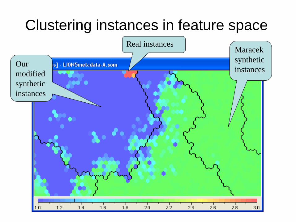
Clustering instances in feature spaceReal instances

Maracek

synthetic

instancesOur

modified

synthetic

instances

Why are the instance classes different?

Clear feedback

for our generator

Visualising footprints

Slack =Total seats available - Total seats required.

SACP handles low slack (tighter) instances better than TSCS.

Maracek instances are not discriminating.

+ve means SACP is better

Conclusions

• We aimed to:

– identify various types of instances within instance space;

– understand the effect of instance generation method on

the properties of the instances;

– visualise the generalisation footprint of each algorithm's

performance behaviours;

– determine the parts of instance space where one

algorithm dominates the other.

• We can now

– identify if the footprint overlaps the kind of instances we

find in the real-world

– Gain insights into strengths and weaknesses

– Use feedback to modify instance generators to suit

requirements (real-world-like, discriminating, etc.)

Next steps

• Mathematically define the footprint boundary

• Develop a set of metrics to define

– the size of a footprint (a measure of good

performance generalisation)

– The degree of overlap with regions of interest (e.g.

real-world instances)

• Develop a tool for researchers to use

– We can then start to demand more comprehensive

reporting of algorithm performance results

– We can analyse the standard benchmark instances

and determine their place in instance space

Smith-Miles, K., Lopes, L.: Measuring Instance Difficulty for Combinatorial

Optimization Problems, Computers and Operations Research, in press.