Generalised Predictive Control(Tuning & Implementation)

Amir Reza Neshasteriz

Peyman Bagheri

Generalized Predictive Control(Tuning & Implementation)

2

• GPC Formulation

• Proposed GPC Method (Camacho & Bordons)

• Extended GPC Method

• Pole Placement Tuning

• Tuning Based on Analysis of Variance (ANOVA)

• GPC application in a PH plant

• Implementation of GPC

Overview of the Presentation

uN

ju

N

Nj

jtujjtrtjtyjJ1

22 )1()()()|(ˆ)(2

1

Introduction to Generalised Predictive Controllers

• CARIMA Model :

)(

)1()()()( 11 tetuqBqtyqA d

• Cost Function :Cost Function :

)()( 11 fyGIGGbHu dTT

• Control Signal :Control Signal :

• Exercising Receding Horizon Concept :

• Applying the input to the system

• Calculating Output with respect to the reference

)()( fyKtu d 11 z

Introduction to Generalised Predictive Controllers

Proposed GPC methodProposed GPC methodBy Camacho & BordonsBy Camacho & Bordons

• First Order System Estimation :

• CARIMA Prediction :

• Calculating Input Sequence :

sdes

KsG

1)( dz

az

bzzG

)1()(

1

11

)1()2(ˆ)1(ˆ)1()(ˆ jtubtjdtyatjdtyatjdty

)1().....()(min

NttuNJ RwPyMu

Proposed GPC methodProposed GPC methodBy Camacho & BordonsBy Camacho & Bordons

• Considering and Receding Horizon Concept :

• Controller Coefficients :

NdN

dN

2

1 1

)(1...1)( trtw

)()1(ˆ)(ˆ)( 121 trltdtyltdtyltu ryy

ak

akkl

iiiyi ˆ

ˆ

321

)(gk ji

AdvantagesAdvantages & Limitations& Limitations

• Advantages and Improvements Compared to conventional method:

1. Less Computational Burden

2. Ability and capacity for utilization in most process applications

3. Simplicity regarding implementation

• Limitations :

1. Application restricted to First order estimates (Oscillating Modes Neglected)

2. Effects of presumable zeros excluded

3. Choosing lambda heuristically

4. Lack of tuning

Solution Second/Higher Order Estimation+Tuning

Extended GPC methodSecond Order Systems

• Second Order System Estimation :

• CARIMA Prediction :

• Calculating Input Sequence :

sdess

zsKsG

))((

)()(

21

dzzaza

zbzbzG

)1)(1(

)(1

2

1

1

2

1

1

01

)2()1(

)3(ˆ)2(ˆ)(

)1(ˆ)1()(ˆ

10

212121

21

jtubjtub

tjdtyaatjdtyaaaa

tjdtyaatjdty

)()1()2(ˆ

)1(ˆ)(ˆ)(

113

21

trltultdtyl

tdtyltdtyltu

ruy

yy

Controller Coefficients

• General Predictor (Equivalent Structure) :

• Converting to Vector-Matrix format :

• Minimizing Cost Function with respect to Input Sequence :

fGuySuHGuy ˆ

)|(ˆ

)|1(ˆ

)|(ˆ

)(

)2(

)1(

)1(

)1(

)(

)|(ˆ

)|2(ˆ

)|1(ˆ

tnty

tty

tty

dntu

dtu

dtu

dNtu

dtu

dtu

tNty

tty

tty

ab

SHG

HGPS,GPλI,GGM

wPuPyPMuT

1

T

0

T

210

Controller Coefficients

• Calculating Input (Receding Horizon) :

• Controller Surfaces are constructed using the following assumptions :

1

210

Mq

wqPuqPyqP

)(

row offirst

tu

1

]99.0:05.0:5.0[,

1.0

) ( 15

21

aa

T

HorizonControlN

s

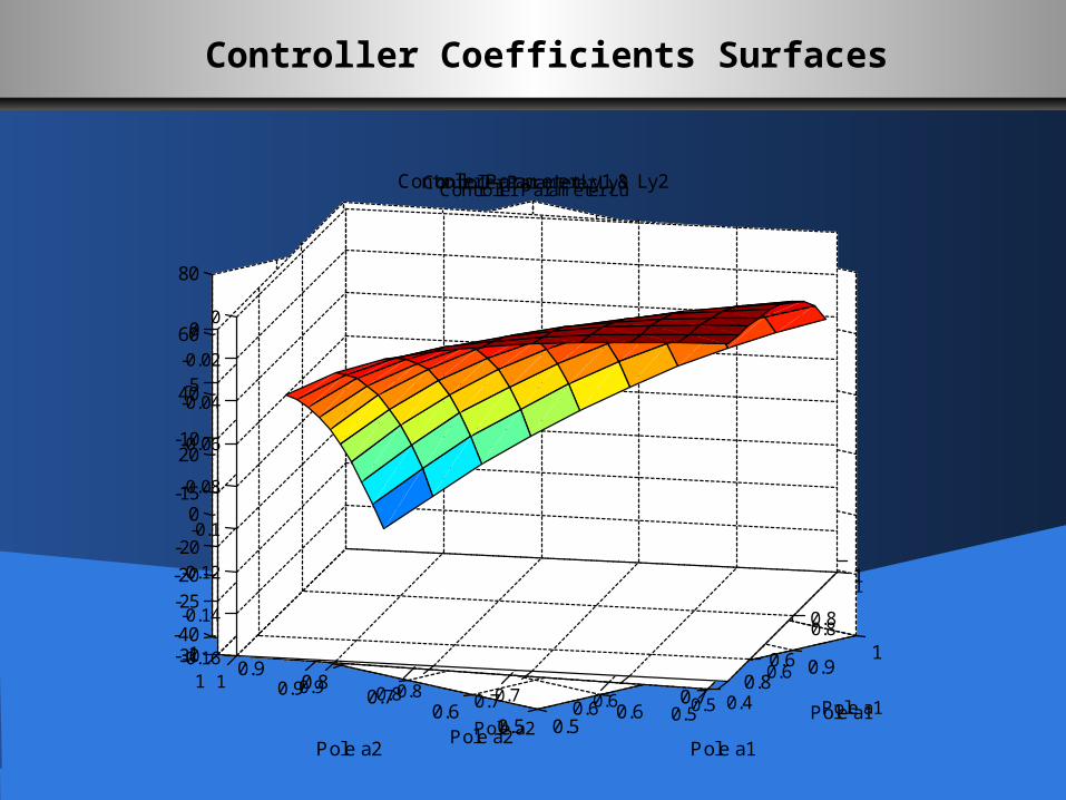
Controller Coefficients Surfaces

0.50.6

0.70.8

0.91

0.50.6

0.70.8

0.91

-40

-20

0

20

40

60

80

Pole a1

Controller Parameter Ly1 & Ly2

Pole a2

Ly1

Ly2

0.4

0.6

0.8

1

0.50.60.70.80.91-30

-25

-20

-15

-10

-5

0

Pole a1

Controller Parameter Ly3

Pole a2

0.6

0.8

1

0.50.60.70.80.91-0.16

-0.14

-0.12

-0.1

-0.08

-0.06

-0.04

-0.02

0

Pole a1

Controller Parameter Lu

Pole a2

Calculating Coefficients Surfaces EstimatesCalculating Coefficients Surfaces Estimates

• As it can be seen in previous plots for the two poles, changes in coefficients are symmetric. Nonlinear Regression of the surfaces yields:

• Iterating for ,the curves for pertaining coefficients are found using MATLAB structure programming

• Estimations for resultant curves are done using Nonlinear Least squares (Levenberg-Marquardt algorithm)

3,2,1,)()(

)()()(),,(),,,(

))(,,()()(),,(

213

212121121

32121211,

iaak

aakkaalaal

kaafkkaal

iiiuyi

iiiuyi

3:01.0:01.0

Table of sub-coefficients

Sub-Coefficient Estimation (Second Order) Sub-Coefficient Estimation (Second Order)

98.0

08.0

:

)(54

232

21

SquareR

SSE

FitofGoodness

pp

pppk ji

Simulation Example (A Non Physical Transfer Function)

1,5.0,15.0

)1()( 4

2

s

s Tess

ssG

0 50 100 150 200 250 300 350 400-2

-1

0

1

2System Response

Time

Out

Put

0 50 100 150 200 250 300 350 400-1

-0.5

0

0.5

1Control Action

Time

Con

trol

Sig

nal

Pole Placement Tuning

uK

yK

sysG yur

Past input gain

Past output gain

PlantSet point gain

rK

• The object of tuning is to find a certain weighting factor λ so that certain criterions, such as performance or stability are met with:

443322,11

443322,11

4321

,,

,,

,,,1)(

1

)()()()(

ggggforfindOR

Update

ggggwhile

ggggPolesKKGz

KKG

GKG

trKtuKtyKtu

uysys

uysys

sysryr

ruy

Simulation Example (A central Heating Configuration of a building)

2

7

21)(

ss

esG

s

0 10 20 30 40 50 60 70-1.5

-1

-0.5

0

0.5

1

1.5

Time (s)O

utpu

t

10 20 30 40 50 60 70

-4

-2

0

2

4

6Control Action

Time (s)

Con

trol

Sig

nal

Comparison between two tuning methods, dotted lines show tuning with and solid line shows proposed tuning method results.

Tuning Based on Analysis of Variance (ANOVA)

• In multi-way ANOVA it is determined whether means in a set of data differ when grouped by multiple factors. If so, it can be verified which factors or combinations of factors are associated with the difference. In other words, the effects of multiple factors on the mean of data are measured.

• To utilize ANOVA for our objective, some experiments have to be performed that involve SOPDT model parameters and tuning factor .

• It should be noted that the tuning procedure is not limited to finding an expression , and for any other parameters in GPC (such as horizons or sampling time) could be repeated.

Experiment Setup

Experiment Setup

• In each of these cases 256 SOPDT models are generated according to the tables.

• In every simulation a tuning parameter that minimizes the following cost function is acquired

• Subsequent to the construction of the bank of models, an analysis of variance is performed on the optimal tuning parameter as a response vector and model parameters as variables. Therefore, model parameters that have more influence on the optimal tuning parameter set could be singled out using ANOVA.

0 0

22 2561 )())()(()( jdttudttrtytC j

ANOVA Results

ANOVA Results

• From the information available from two simulations and their analysis of variance results, optimal λ set will depend on mentioned model parameters in each simulation and hence it is a function of them.

• To find this function, nonlinear regression has to be performed on the and model parameters. After many attempts, the following expression was derived for the real pole case with very good fit

• For the complex conjugate case, the expression is

54

2

1

)()(

)(213

21

21

pp

pp

ppopt

5421 )()()( 3 nnnopt

Illustrative Examples

5.05.1)(

21

ss

esG

s

122)(

2

5

2

ss

esG

s

0 5 10 15 20 25 30 35 40-4

-2

0

2

4

Out

put

0 5 10 15 20 25 30 35 40-6

-4

-2

0

2

4C

ontr

ol s

igna

l

Time(s)

Case Study 1 simulationsolid line: proposed tuning method, Dotted line: conventional method

0 10 20 30 40 50 60

0

0.2

0.4

0.6

Out

put

0 10 20 30 40 50 60-2

-1

0

1C

ontro

l Sig

nal

Time (Samples)

Case Study 2 simulation (the gas fire burner), solid line: proposed tuning method, Dotted line: Trial and Error Method

Performance Comparison

آزمایشگاهی pHسیستم

24

مقدمه

pHفرآیند سازی و کنترل رگوله مساله•

غیرخطی گری شدید، نامعینی مدل و تاخیر زیاد •

pH مدل سازی و کنترل تک ورودی- تک خروجی سیستم •

pHسیستم کنترل چندمتغیرهمدل سازی و •

کارهای راهبه وسیله pHبهبود عملکرد سیستم کنترل •

چندمتغیره

کنترل پیش بین تعمیم یافته•

pHروی سیستم GPCنتایج عملی پیاده سازی •

25

pHفرآیند

pHگ6یری ب6رای مق6دار ی6ک معی6ار ان6دازهغلظت ی6ون هی6درونیوم در محل6ول

آبی است.][ H

:pHدو دسته بندی کلی برای فرآیند

قرار دارد.محلول درون مخزن بسته(: batchبسته ) • .جریان خروجی است pHهدف کنترل پیوسته: •

26

pHمدل سازی دینامیکی فرآیند

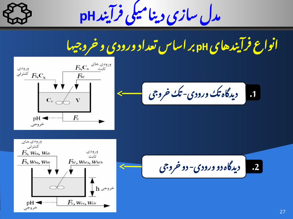
دیدگاه تک ورودی- تک . . 11 خروجی

دیدگاه دو ورودی- دو . . 22 خروجی

بر اساس تعداد ورودی و خروجیها pHانواع فرآیندهای

27

pHمدل سازی دینامیکی فرآیند

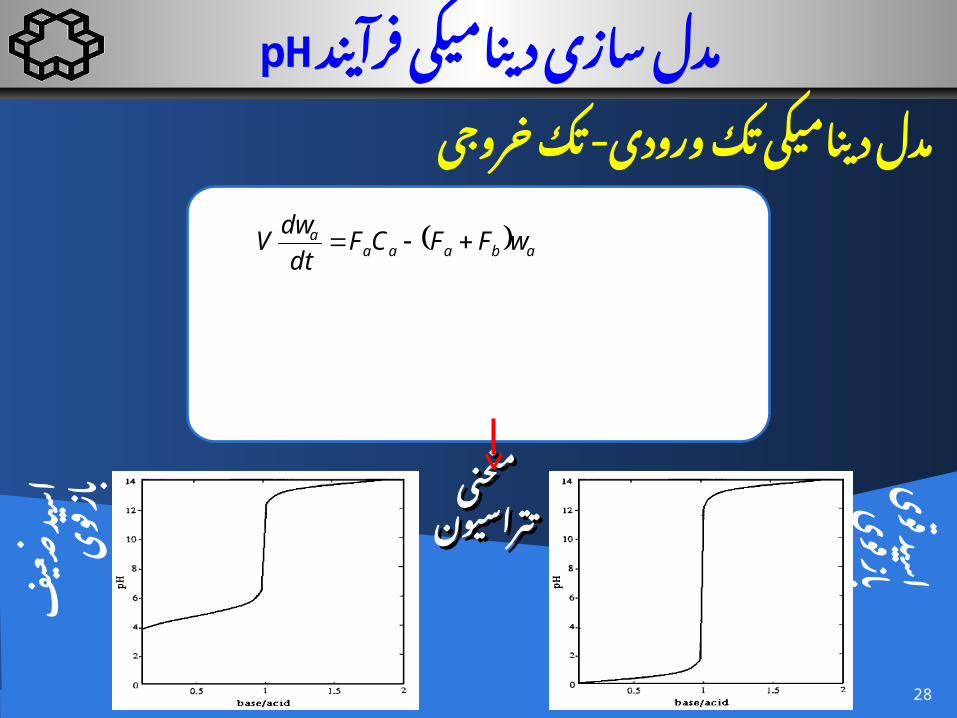
مدل دینامیکی تک ورودی- تک خروجی

abaaaa wFFCF

dt

dwV

منحنیمنحنی

تتراسیتتراسید ونون

سیا

فعی

ضز

بای

وق

سید ا

یوق

باز ی

وق

28

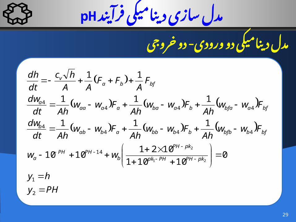
pHمدل سازی دینامیکی فرآیند

PHy

hy

ww

FwwAh

FwwAh

FwwAhdt

dw

FwwAh

FwwAh

FwwAhdt

dw

FA

FFAA

hc

dt

dh

pkPHPHpk

pkPH

bPHPH

a

bfbbfbbbbbababb

bfabfababaaaaaa

bfbav

2

1

14

4444

4444

010101

10211010

111

111

11

21

2

مدل دینامیکی دو ورودی- دو خروجی

29

30

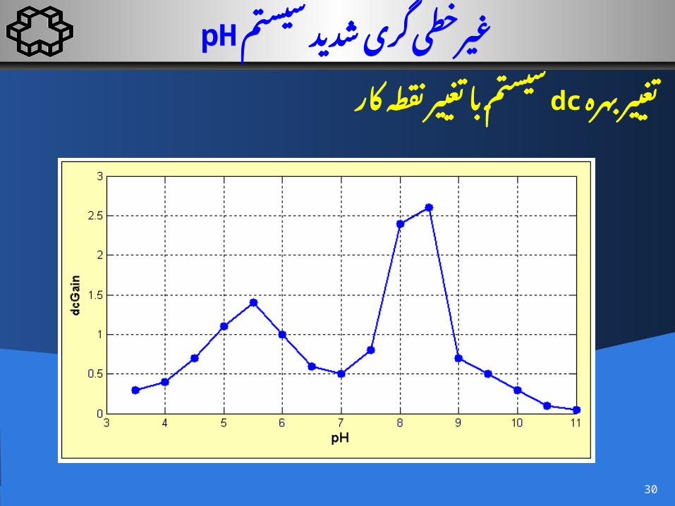
سیستم با تغییر نقطه کار dcتغییر بهره

pHگری شدید سیستم غیرخطی

ورودی-روشهای کنترلی برای حالت تک تک خروجی

مقاالت فراوانی داده شده است، SISOبرای حالت روشهایی که بیشتر مورد استفاده قرار گرفته:

کنترل پیش بین مدل چندگانه•کنترل پیش بین تعمیم یافته مدل چندگانه•کنترل تطبیقی مدل چندگانه•کنترل فازی پیش بین مدل•کنترل تطبیقی عصبی•کنترل مقاوم •الگوریتم ژنتیک•و ...•

31

: SISOنقص کنترل بسته میشود. pHحلقه کنترلی روی کانال •در عمل نیاز داریم حجم مخزن ثابت بماند.•

کاری که در آزمایشگاه انجام میشود:کنترل سطح محلول با فیدبک داخلی توسط آب

در اثر افزودن آب pH تغییر

32

ورودی-روشهای کنترلی برای حالت تک تک خروجی

تداخل

3333

ساختار کنترلر برای سیستم خطی چندمتغیره:

SISOساختارهای دکوپله ساز و کنترلرهای •

ساختار کنترلی چندمتغیره•کنترل پیش بین کنترلرهای هوشمند

و ...

تعمیم بین پیش تعمیم کنEEترل بین پیش کنEEترل ((GPCGPC))یافته یافته

مEEدل بین پیش مEEدل کنEEترل بین پیش کنEEترل ((MPCMPC))

روشهای کنترلی فرآیند pHچندمتغیره

34

(GPC)کنترل پیش بین تعمیم یافته

GPCGPC بدون پیچیدگی زیاد بدون پیچیدگی زیاد MIMOMIMOو و SISOSISO قابل استفاده برای سیستمهای قابل استفاده برای سیستمهای •constrainsconstrains امکان بکارگیری امکان بکارگیری •قابل استفاده برای سیستمهای تاخیردارقابل استفاده برای سیستمهای تاخیردار • مقاوم بودن روش کنترلی نسبت به تغییر پارامترها مقاوم بودن روش کنترلی نسبت به تغییر پارامترها•

کنترل پیش بین تعمیم یافته (GPC)

35

MIMO state space model: MIMO state space model: x(k+1) = A x(k) + B u(k)x(k+1) = A x(k) + B u(k)y(k) = C x(k) + D u(k) + dist Note: Assumes y(k) = C x(k) + D u(k) + dist Note: Assumes D=0D=0

J = sum (r-y)^2 + (u(k+i-1)-uss) R (u(k+i-1)-uss)J = sum (r-y)^2 + (u(k+i-1)-uss) R (u(k+i-1)-uss)

umin < ufut < umaxumin < ufut < umaxDumin < Dufut < DumaxDumin < Dufut < Dumax

در فضای حالتدر فضای حالت GPCGPCفرموله بندی فرموله بندی

استفاده از مطلب برای کنترل pHسیستم

36

عملی بدست آمده نتایج

37