Prepared for submission to JCAP

Generalised form factor dark matter inthe Sun

Aaron C. Vincent,1 Aldo Serenelli2 and Pat Scott3

1Institute for Particle Physics Phenomenology (IPPP), Department of Physics, DurhamUniversity, Durham DH1 3LE, UK

2Institut de Ciencies de l’Espai (ICE-CSIC/IEEC), Campus UAB, Carrer de Can Magranss/n, 08193 Cerdanyola del Valls, Spain

3Department of Physics, Imperial College London, Blackett Laboratory, Prince ConsortRoad, London SW7 2AZ, UK

E-mail: aaron.vincent@durham.ac.uk, aldos@ice.csic.es, p.scott@imperial.ac.uk

Abstract. We study the effects of energy transport in the Sun by asymmetric dark matterwith momentum and velocity-dependent interactions, with an eye to solving the decade-old Solar Abundance Problem. We study effective theories where the dark matter-nucleonscattering cross-section goes as v2nrel and q2n with n = −1, 0, 1 or 2, where vrel is the darkmatter-nucleon relative velocity and q is the momentum exchanged in the collision. Suchcross-sections can arise generically as leading terms from the most basic nonstandard DM-quark operators. We employ a high-precision solar simulation code to study the impact onsolar neutrino rates, the sound speed profile, convective zone depth, surface helium abun-dance and small frequency separations. We find that the majority of models that improveagreement with the observed sound speed profile and depth of the convection zone also reduceneutrino fluxes beyond the level that can be reasonably accommodated by measurement andtheory errors. However, a few specific points in parameter space yield a significant overallimprovement. A 3–5 GeV DM particle with σSI ∝ q2 is particularly appealing, yieldingmore than a 6σ improvement with respect to standard solar models, while being allowed bydirect detection and collider limits. We provide full analytical capture expressions for q- andvrel-dependent scattering, as well as complete likelihood tables for all models.

arX

iv:1

504.

0437

8v1

[he

p-ph

] 1

6 A

pr 2

015

Contents

1 Introduction 11.1 Dark matter in the Sun 21.2 Generalised form factor dark matter 3

2 Capture of dark matter by the Sun 52.1 Standard (velocity and momentum independent) treatment 52.2 Velocity and momentum-dependent treatment 62.3 The geometric limit 8

3 Conductive energy transport by dark matter 8

4 The DarkStec solar dark matter code 114.1 Annihilation 12

5 Limits on generalised form factor dark matter from solar physics 135.1 Saturation of capture 135.2 Solar neutrino fluxes 145.3 Depth of the convection zone 195.4 Surface helium abundance 225.5 Sound speed profile 225.6 Frequency separation ratios 235.7 Combined limits 27

6 Discussion 326.1 Solving the Solar Abundance Problem 326.2 Comparison with collider and direct limits 336.3 Comparison with previous work 34

7 Conclusions 36

1 Introduction

A non-relativistic relic dark matter particle, with a mass of a few GeV or more, is theleading candidate to explain astrophysical and cosmological phenomena ranging from clusterkinematics and galactic rotation curves, to gravitational lensing and the heights and positionsof the acoustic peaks in the cosmic microwave background. Dark matter (DM) may havebeen produced in a similar way to Standard Model (SM) particles, either via chemical freeze-out (as in the weakly-interacting massive particle – WIMP – scenario) or via an initialasymmetry, analogous to baryogenesis (as in the asymmetric DM – ADM – scenario). Ifeither of these scenarios is correct, it is possible that DM interacts weakly with SM particles.Such interactions would be seen most easily as a small elastic scattering cross-section betweenDM and quarks.

The search for DM-quark interactions has been the focus of terrestrial direct detectionexperiments such as DAMA [1], CoGeNT [2], CRESST-II [3] and CDMS II [4], who have allreported excess events above their expected backgrounds. On the other hand, XENON10 [5],

– 1 –

XENON100 [6], COUPP [7], SIMPLE [8], LUX [9] and SuperCDMS [10] have all establishedstrong limits on the DM-nucleon cross-section, seemingly in contradiction to the excessesobserved by other experiments. These underground detectors are typically most sensitive toDM particles with masses of order mχ = 50 to 100 GeV, which lead to the largest recoilenergies on the heavy nuclei used as targets. For the same reason, they are also best suitedto probing fast-moving DM particles, resulting in a threshold velocity of a few tens of km s−1

for an incoming DM particle to create a nuclear recoil event.Collisions between DM and nuclei can also lead to capture and accumulation of DM

in the solar core. For this to occur, collisions between DM and nuclei in the Sun mustresult in sufficient energy transfer for the DM velocity to be brought below the local escapevelocity. The kinematic region probed by the Sun is quite different to the one probed by directdetection: optimal energy transfer, leading to optimal capture rates, occurs for DM particlemasses closely matching the solar composition, i.e. a few GeV. Because DM gains speed asit falls into the solar potential well, the low-velocity tail of the local DM distribution is thedominant contributor to solar capture; the opposite is true for direct detection experiments.Direct detection and solar physics are therefore highly complementary laboratories for thestudy of DM-quark scattering.

1.1 Dark matter in the Sun

The effect of DM on stars has been the subject of investigation for some time (see [11–13]for reviews). There are two main scenarios where DM might create observable effects on theSun: 1) the capture and annihilation of WIMP-like particles; and 2) the accumulation ofan “asymmetric” species. The first case is characterised mainly by a search for high-energyneutrinos with Eν ∼ mχ [14–31] and MeV-scale decay products [32, 33], using detectors suchas IceCube and SuperKamiokande. Annihilation of DM in a star can also provide an energysource through the release of other SM particles [11, 34–47], leading to changes in the corestructure. The capture rate of DM in the Sun is however far too low for the energy releasedthis way to have any significant effect on solar structure [11].

Our focus in this paper is therefore on the case where DM either cannot annihilate, ordoes so far more slowly than it is captured. In this case DM is effectively asymmetric (i.e.ADM), and large quantities of DM may have built up inside the Sun over its lifetime. Theweak interactions of DM with quarks give the DM particles relatively large inter-scatteringdistances, making them potentially significant conductors of energy. Just like the captureprocess, energy transfer is most efficient for lighter DM masses (1− 10 GeV), as momentumtransfer is maximised when the masses of the colliding particles are equal, and the Sunis mostly H (A = 1) and He (A = 4). It is interesting to note that this is roughly themass range expected in the most common models of ADM [48], in order to explain the1:5 cosmological relic baryon-to-DM density ratio. In contrast, earth-based direct detectionexperiments lose sensitivity in this range, as they make use of high-mass elements such asgermanium (A ∼ 72) and xenon (A ∼ 131), for which high incoming DM velocities arenecessary to create a measurable recoil.

There is a window of elastic DM-nucleon scattering cross-sections [49–53] at σ ∼ 10−36

cm2 for spin-independent (SI) couplings (10−34 cm2 in the spin-dependent – SD – case) forwhich σ is large enough to allow sizeable capture of DM, but small enough that the meaninterscattering distance is still large. A large inter-scattering distance allows heat to beredistributed away from the solar core by DM-nucleon scattering. This has the effect ofreducing the temperature of the solar core Tc, and increasing the central density and pressure.

– 2 –

Changes of state variables near the solar centre affect the production of neutrinos fromfusion processes, especially the flux of 8B neutrinos, which goes as T βc with β ∼ 20–25. Thetemperature and density changes in the core reduce the local sound speed, and force anoverall mass redistribution that impacts the solar structure at other radii. This leads tomodifications of the sound speed profile over the entire depth profile of the Sun, and shiftsthe height of the base of the convection zone. Both the sound speed profile and the depth ofthe convection zone have been independently measured using helioseismology.

It has been shown that high-precision solar evolution models including capture, trans-port and (minimal) annihilation of DM can be built to satisfy the observed solar age, radius,and luminosity [51–53]. At the same time, it appears possible for the inclusion of DM insuch models to affect the (less well constrained) 8B flux in an observable way, and evenimprove agreement with the observed sound speed profile and the depth of the convectionzone. Neither of these latter two observables are well reproduced by standard solar modelscomputed with the latest surface compositions [54–59]. This issue, known as the “solar com-position” or “solar abundance” problem, has been brought about by the 20–25% reductionin the measured solar metallicity in recent years [60–71], and is one of our motivations forthis paper.

Although several studies have indicated that ADM can alleviate some of this tension,the cross-sections required to do so are typically far higher than allowed by limits from directdetection. Here we investigate whether broader consideration of the kinematic structure ofthe DM-nucleon vertex might provide a way around this. In the process, we provide firstrigorous limits from solar physics on such DM models, which we refer to as ‘generalisedform factor dark matter’. In a separate paper [72] we discussed a specific realisation ofmomentum-dependent dark matter that leads to a 6σ improvement over the Standard SolarModel (SSM). We revisit this model in Sec. 6.1.

1.2 Generalised form factor dark matter

The kinematic differences between direct detection and the Sun become even more markedif the DM-nucleon interaction is not assumed to be independent of the DM-nucleon relativevelocity, or the momentum transferred in the collision. There is indeed no guarantee thatthe standard SI and SD operators correctly represent the DM-quark interaction. In particlephysics, the interaction cross-section generally depends on the centre of mass energy and thetransferred momentum, parameterised using the Lorentz-invariant Mandelstam variables s, tand u. In the non-relativistic limit, these become the centre of mass momentum, proportionalto the relative velocity vrel, and the transferred momentum q = ∆p. As these are smallquantities, the constant term usually dominates in a series expansion of the cross-section.However, many models with non-trivial dependencies on vrel and q exist, typically motivatedby theoretical arguments or attempts to reconcile experimental results.

To make quantitative predictions, a specific form of σ(vrel, q) must be chosen. Becausewe wish to remain as general as possible, we choose to focus on couplings of the form σ ∝ v2nreland σ ∝ q2n, with n = −1, 1, 2. The v2rel and v4rel forms are respectively called p-wave andd-wave interactions, and correspond to the cases where the initial state particles possess 1 and2 units of relative angular momentum, respectively. These are always present, but normallyonly dominate when all lower-order terms in the scattering matrix element – including theconstant (s-wave) term – are suppressed due to cancellations. Cross-sections depending on qcan arise, for example, from a non-zero particle radius (the analogue of a nuclear form factor),from parity-violating couplings like χγ5χQQ, χγµγ5χQγ

µQ and χσµνγ5χQσµνQ, or from a

– 3 –

small anapole or dipole interaction between the dark and visible sectors [73–85]. We refer tothe class of models where DM-nucleon scattering cross-sections depend on some combinationof q and/or vrel as ‘generalised form factor DM’ because it generalises the effects of formfactors to arbitrary powers of q and vrel.

Concretely, we focus on the couplings

σ = σ0

(q

q0

)2n

(1.1a) and σ = σ0

(vrelv0

)2n

. (1.1b)

These can lead to either spin-dependent (SD) or spin-independent (SI) interactions, depend-ing on the axial structure of the DM-nucleon interaction vertex. The normalisation σ0 mustbe defined with respect to some reference velocity v0 or momentum q0. We will choosev0 = 220 km s−1, the typical halo DM velocity, and q0 = 40 MeV, corresponding to a nuclearrecoil energy of around 10 keV in an underground direct detection experiment.

The DM-nucleus cross-section is related to the above DM-nucleon cross-sections via:

σN,i =m2

nuc(mχ +mp)2

m2p(mχ +mnuc)2

[σSIA

2i + σSD

4(Ji + 1)

3Ji|〈Sp,i〉+ 〈Sn,i〉|2

], (1.2)

where Ai and Ji are respectively the atomic number and total angular momentum of nuclearspecies i; 〈Sp,i〉 and 〈Sn,i〉 are the spin expectation values of its proton and neutron systems.Given the A2 dependence of Eq. 1.2 we will find that, in spite of the Sun’s small metallicity,spin-independent DM can have a significantly larger effect than a spin-dependent DM candi-date, which couples mostly to hydrogen. This fact has not been emphasised very much in theliterature. The full effect of a momentum-dependent cross-section will furthermore dependcrucially on the composition of heavier elements.

The full impact of momentum and velocity-dependent DM on solar observables has notbeen studied before. The authors of Ref. [30] computed the effect of such couplings on the cap-ture rate of spin-dependent DM, and computed neutrino fluxes from an annihilating species.However, they did not include a treatment of heavier elements, nor of the crucial energy trans-port by DM once captured. In Refs. [86, 87], the authors computed capture and transportrates for ADM models with long-range interactions. To account for the impacts of the non-trivial scaling of these cross-sections with momentum and velocity, they employed effectivecross-section scaling factors to decouple the cross-sections entering the capture and transportcalculations, and avoid modifying the standard velocity-and-momentum-independent treat-ment of capture and energy transport. As we show later, it happens that this rescaling canindeed be done without any loss of generality for capture in the velocity-dependent case, butit is not possible in the momentum-dependent case. It is also not possible to account for theeffects on energy transport of either a velocity or momentum dependence in this manner;rather, a full recalculation of the transport coefficients must be performed [88].

The structure of this paper is as follows: in Section 2, we review the capture equationsfor DM in the Sun, and present the necessary modifications for velocity and momentum-dependent scattering of DM with nucleons. In Section 3 we review the theory of conductiveheat transport by DM developed in Refs. [88, 89], along with its application to solar modelling.Section 4 describes the DarkStec computer code that we have developed for simulating theeffects of generalised form factor DM on the Sun. We present results in Section 5, and discusstheir implications with regards to the Solar Abundance Problem, current experimental limitsand previous work on the topic in Section 6. We summarise in Section 7.

– 4 –

2 Capture of dark matter by the Sun

2.1 Standard (velocity and momentum independent) treatment

The population of DM particles in the Sun Nχ(t) is follows the differential equation

dNχ(t)

dt= C(t)−A(t)− E(t), (2.1)

where C(t) is the capture rate, A(t) is rate at which annihilations occur and E(t) representsevaporation. Unless DM is strongly self-interacting (not the case we consider here, butdiscussed in Ref. [90]), C(t) does not depend on the DM population already capturedby the Sun. A(t) is the rate of annihilation, and is proportional to the square of the DMpopulation. Here we consider the case where DM is fully asymmetric, so A(t) = 0, althoughwe comment briefly in Section 4.1 on the implications of allowing DM to self-annihilate.

Evaporation occurs when a DM particle gains enough energy from a scattering event toovercome the Sun’s gravitational potential and escape, so E(t) is linear in the DM population(being simply the product of the single-particle evaporation probability and the number ofcandidates for evaporation). Evaporation requires a significant gain in momentum, as thetypical velocity of a thermalised DM particle is ∼100 km s−1, whereas the escape velocity inthe solar core approaches 1400 km s−1. This means that evaporation is only significant if DMis similar in mass to the nucleus with which it scatters in the Sun. In practice this means thatDM about the mass of helium (4 GeV) and lighter is typically most prone to evaporation, butother masses closely matched to significant elements in the Sun (C, N, O, Fe =⇒ mχ ∼ 12,14, 16, 56 GeV) can also in principle be affected [91]. The evaporation rate depends on theinteraction cross-section, mean free path and thermal regime (LTE vs Knudsen); extendingthe standard analyses to generalised form factor DM is therefore non-trivial. In practicethe rate of evaporation is extremely low in almost all cases where the nuclear scatteringcross-section is allowed by direct detection; for very specific analyses it should be taken intoaccount, but for the purposes of this paper we assume that the evaporation rate is zero. Weintend to return to this point in detail in a future paper.

We now turn to the capture rate as it is implemented in our simulations. As we areusing the DarkStars code [92], we closely follow Refs. [11, 93]. We take the local distributionfunction f(u) of DM to be Maxwell-Boltzmann, with dispersion u0 = 270 km s−1. In theframe of the Sun, moving at u = 220 km s−1 relative to the Galactic rest frame,

f(u) =

(3

2

)3/2 4ρχu2

π1/2mχu30exp

(−

3(u2 + u2)

2u20

)sinh(3uu/u

20)

3uu/u20. (2.2)

As it falls into the gravitational potential well of the Sun, a DM particle acquires a velocityw =

√u2 + v2esc(r, t). It becomes gravitationally captured by the Sun if it loses enough

kinetic energy in a scattering event for w to fall below the local escape velocity vesc(r, t). Forthis to occur, the fractional energy lost by the DM particle ∆ = 2ER/mχw

2, correspondingto nuclear recoil energy ER, must be in the interval

u2

w2≤ 2ER

mχw2≤ µ

µ2+, (2.3)

where µ ≡ mχ/mnuc and µ± ≡ (µ ± 1)/2. The local capture rate of particles with velocityw is the sum over nuclear species at radius r, of the rate of scattering in the interval of Eq.

– 5 –

2.3, i.e.

Ω(w) = w∑i

σN,ini(r, t)µ2i,+µi

Θ

(µiv

2

µ2i,−− u2

)∫ mχw2µi/2µ2i,+

mχu2/2|Fi(ER)|2 dER, (2.4)

where |Fi(ER)|2 is the nuclear form factor. For hydrogen this is a constant, whereas forheavier nuclei we use the usual Helm form factor

|Fi(ER)|2 = exp

(−ER

Ei

). (2.5)

Here Ei is a constant quantity for each nuclear species i, given by

Ei =5.8407× 10−2

mN,i(0.91m1/3N,i + 0.3)2

GeV. (2.6)

Integrating over the phase space, the total capture rate of DM in the Sun is then

C(t) = 4π

∫ R

0r2∫ ∞0

f(u)

uwΩ(w) dudr. (2.7)

For a constant cross-section and a Maxwell-Boltzmann velocity distribution, this can besolved analytically [11, 93]. However, in the following we generalise the above equations toallow momentum and velocity-dependent σSI and σSD.1 In this case, numerical integrationbecomes necessary.

2.2 Velocity and momentum-dependent treatment

We begin with a momentum-dependent cross-section of the form Eq. 1.1a, with σ ∝ q2n. Toinclude such a cross-section in Eq. 2.4, the constant cross-section must be replaced with Eq.1.1a and the dependence on the nuclear recoil energy moved inside the form-factor integral.This explicitly illustrates the equivalence of a momentum-dependent cross-section to a changein form factor, and we refer to the corresponding integral and associated multiplicative factorsas the ‘generalised form factor integral’ (GFFI). For hydrogen, |F (ER)|2 = µ2+/µ, so thechange required is

GFFIn=0 =

∫|F (ER)|2 dER → GFFIn6=0,H =

(p

q0

)2n 1

µn

∫ µ/µ2+

u2/w2

µ2+∆n

µd∆, (2.8)

where we have expressed the form factor integral in terms of ∆ instead of ER for compactness.We do this by noting that the transferred momentum is q =

√2mnucER, so the fractional

energy change can be written ∆ = µq2/p2, where p = mχw is DM particle’s incomingmomentum. Performing the integral in Eq. 2.8 yields

GFFIn6=0,H =

(p

q0

)2n µ2+µn+1

1

1+n

[(µµ2+

)n+1−(u2

w2

)n+1], (n 6= −1)

ln(µµ2+

w2

u2

), (n = −1)

(2.9)

1We will use σ as a shorthand for either σSI or σSD, as the spin and kinematic dependence can be factorised.For an explicit treatment, see [94].

– 6 –

100

101

10−6

10−4

10−2

100

102

104

mχ (GeV)

Fcapture

σ ∝ q−2

σ ∝ q2

σ ∝ q4

100

101

10−6

10−4

10−2

100

102

104

mχ (GeV)

Ftransp

ort

σ ∝ q−2

σ ∝ q2

σ ∝ q4

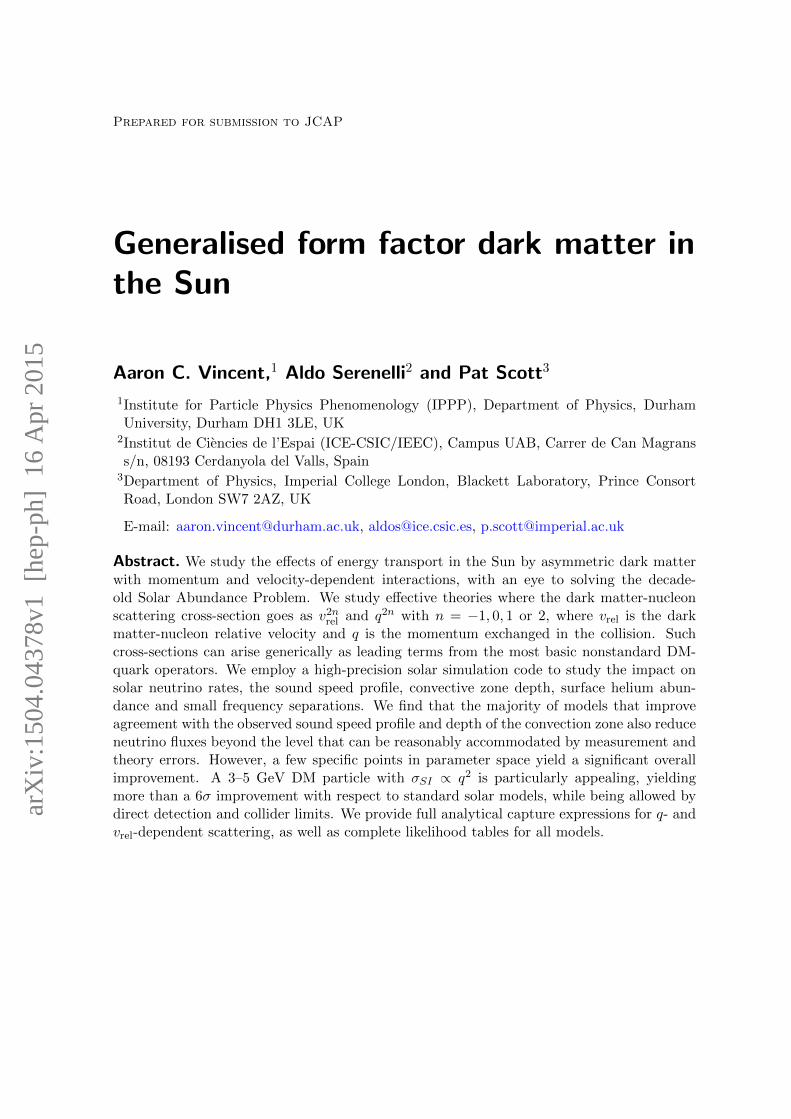
Figure 1. Left: effective enhancement/suppression of DM capture in a standard model of the Sun(AGSS09ph; [59]), due to a momentum-dependent cross-section, as computed with Eq. 2.11. Theblack line at F = 1 corresponds to σ = const. Solid lines are spin-independent (SI) and dashed linesare spin-dependent (SD), coupling only to hydrogen. Right: effective enhancement/suppression ofenergy transport as defined in Eq. 3.10 , in the LTE regime, with σ0 = 10−35 cm2. We note thataway from LTE, the behaviours reverse, and a q−2 cross-section actually yields an enhancement withrespect to the constant case. This can be seen in Fig. 2. The full effect of a q-dependent cross-sectionis then the combined effect of the left and right-hand panels.

For heavier elements, the integrand includes the Helm form factor (Eq. 2.5), so

GFFIn6=0,i 6=H =

(p

q0

)2n µ

(Bµ)1+n

[Γ

(1 + n,B

u2

w2

)− Γ

(1 + n,B

µ

µ2+

)], (2.10)

where B ≡ 12mχw

2/Ei, and Γ(m,x) is the (upper) incomplete gamma function. To gain amore intuitive understanding of Eqs. 2.9 and 2.10 we show in Fig. 1 the overall enhancementor suppression to the capture rate with respect to the constant case,

Fcapture =

∑i fiA

2iGFFIn6=0,i∑

i fiA2iGFFIn=0,i

, (2.11)

for three values of n 6= 0. In this example we just take w = w(r = 0) and use the present-dayAGSS09ph Standard Solar Model2 [59, 68]. Here fi represents the fractional composition ofeach species with atomic number Ai. For the spin-dependent cross-sections, the sum overthe species i only includes hydrogen. Of course the actual capture rate must be accuratelyintegrated over the entire star, and we compute it precisely with Eq. 2.7 in our simulation.In each case, the overall behaviour roughly follows the (p/q0)

2n dependence, as heavier DMwill have gained more momentum as it falls into the solar gravitational well.

In the velocity-dependent case (Eq. 1.1b), where σ ∝ v2nrel, the modification to thecapture rate is much simpler. The partial capture rate Ω(w) ∝ σ is simply transformed bythe replacement

σ → σ0

(w

v0

)2n

. (2.12)

2Publicly available at http://www.ice.csic.es/personal/aldos/Solar_Models.html.

– 7 –

The integral Eq. 2.7 can then be evaluated to obtain the modified capture rate. We latershow with our solar simulation code that the enhancement due to velocity-dependence agreesvery well with what is obtained using the standard (n = 0) treatment and an average of thecross-section throughout the volume of the star

σ(vrel) ' 〈σ(w0)〉 =1

M4π

∫ R

0σ(w0)ρ(r)r2 dr, (2.13)

where w0 ≡√v20 + v2esc(r) is the typical velocity acquired by an in-falling WIMP as it reaches

radius r. This indicates that a cross-section proportional to v2 or v4 – typically thought ofas a suppression – actually yields a considerable enhancement. We note that σ(vrel) has beenerroneously approximated to σ(〈w0〉) rather than 〈σ(w0)〉 in the literature [87], although[vesc(r = 0)/v0]

2n does at least provide the correct enhancement to the capture rate to withina factor of a few.

2.3 The geometric limit

In all cases, the total effective cross-section of the Sun to collisions with DM particles cannotexceed the geometric “cutoff”

σmax = πR2(t), (2.14)

which corresponds to the case where the Sun is optically thick to DM. This places a funda-mental limit on the capture rate

Cmax(t) = πR2(t)

∫ ∞0

f(u)

uw2(u,R) du (2.15)

=1

3πρχmχ

R2(t)

(e− 3

2

u2u20

√6

πu0 +

6GNM +R(u20 + 3u2)

RuErf

[√3

2

uu0

]).

The actual capture rate to be used must therefore be the lesser of Eqs. 2.15 and 2.7. Assuminga steady radius and a local DM density of ρχ ' 0.38 GeV cm−3, the maximum amount ofDM that can accumulate in the Sun by its current age is therefore

Nχ,max ' 1.5× 1047(

GeV

mχ

)' 1.3× 10−11

(GeV

mχ

)Nb, (2.16)

where Nb 'M/mp is the total number of baryons in the Sun.

3 Conductive energy transport by dark matter

If enough DM is captured by the Sun, its large typical inter-scattering distance lχ means thatit is a more efficient carrier of heat over long distances than ordinary baryonic material, so itcan act as an additional mechanism for heat transport alongside photons. The formalism weuse to compute the effect of microscopic energy transport by DM conduction was developedby Gould and Raffelt [89]. By solving a perturbative expansion of the Boltzmann collisionequation (BCE) in the Sun’s gravitational potential, they showed that the thermal conductionby a weakly-interacting species can be expressed in terms of two quantities: a dimensionlessmolecular diffusivity α(µ), and thermal conductivity κ(µ), where µ ≡ mχ/mnuc is again theratio between the DM and nucleon masses. If more than one nuclear species is present, α

– 8 –

and κ get replaced with effective values, which are weighted by the number densities of eachspecies in the plasma mixture at each height in the Sun.

In the local thermal equilibrium (LTE) regime, where lχ(r) is much smaller than boththe inverse of the local temperature gradient |∇ lnT (r)| and the DM scale height rχ, thevalues of α and κ are found by solving the first order expansion of the BCE. This is donein terms of the quantity ε ≡ lχ(r)|∇ lnT (r)|, via the formal inversion of the Boltzmanncollision operator C(u, r), where C(u, r)F (u, r) represents the net change in the DM phasespace distribution F (u, r) due to collisions with nuclei. The collision operator is definedvia phase space integrals over collision rates, meaning that the dependence of the collisionalcross-section σ on vrel and q must be explicitly included in the calculation. In Ref. [89] Gouldand Raffelt computed and tabulated α(µ) and κ(µ) for a constant scattering cross-section(n = 0). In Ref. [88], we extended the formalism to include velocity and momentum-dependent cross-sections (n 6= 0), showing that the resulting changes in α, κ and lχ can havepotentially large effects on heat transfer in the Sun.

The equilibrium distribution of DM particles in the gravitational potential φ(r) of thesun is given by [11, 88, 89]

nχ,LTE(r) = nχ,LTE(0)

[T (r)

T (0)

]3/2exp

[−∫ r

0dr′

kBα(r′) dT (r′)dr′ +mχ

dφ(r′)dr′

kBT (r′)

], (3.1)

where r = 0 represents the centre of the Sun. The conductive luminosity is:

Lχ,LTE(r) = 4πr2ζ2n(r)κ(r)nχ,LTE(r)lχ(r)

[kBT (r)

mχ

]1/2kB

dT (r)

dr. (3.2)

where the factor ζ2n accounts for a velocity-dependent [ζ = v0/vT (r)] or momentum-dependent[ζ = q0/mχvT (r)] cross-section, and vT (r) ≡

√2kBT (r)/mχ is related to the typical thermal

velocity [89]; v0 and q0 are respectively the reference velocity and momentum defined in Eq.1.1. The rate of energy transported per unit mass of stellar material is:

εχ,LTE(r) =1

4πr2ρ(r)

dLχ,LTE(r)

dr. (3.3)

This quantity is usually expressed in units of ergs g−1 s−1.If the condition lχ rχ is violated, LTE is no longer valid and the system exists in the

Knudsen regime of non-local transport, where the DM distribution is essentially isothermal.It was shown in Refs. [89, 95] by Monte Carlo simulation that Eqs. 3.1 and 3.2 can be correctedto properly account for a large Knudsen number K ≡ lχ/rχ. Here we have formally defined

rχ =

(3kBTc

2πGρcmχ

)1/2

. (3.4)

Following [11, 50], we define:

h(r) =

(r − rχrχ

)3

+ 1, (3.5)

f(K) =1

1 +(KK0

)1/τ , (3.6)

– 9 –

10−40

10−38

10−36

10−34

10−32

10−30

10−16

10−14

10−12

10−10

10−8

10−6

10−4

σ0 (cm−2)

∫r2|ǫ(r,σ)|dr

σ = const.σ ∝ q−2

σ ∝ q2

σ ∝ q4

10−40

10−38

10−36

10−34

10−32

10−30

10−16

10−14

10−12

10−10

10−8

10−6

10−4

σ0 (cm−2)

σ = const.

σ ∝ v−2

σ ∝ v2

σ ∝ v4

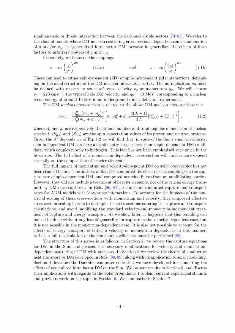
Figure 2. Illustration of the transition from the local thermal equilibrium (LTE) to the Knudsen(non-local, isothermal) regime of energy transport by DM scattering, for momentum-dependent (left)and velocity-dependent scattering (right). Leftwards of the peak in each curve corresponds to theKnudsen regime, whereas rightwards is the LTE regime. The total energy transport is plotted for afixed DM mass (mχ = 10 GeV) and number ratio of DM to baryons (nχ/nb = 10−15). Solid lines arespin-independent couplings, whereas dashed lines represent the spin-dependent case where the DMscatters only on hydrogen. This has the effect of increasing the mean free path, leading to a transitionto the Knudsen regime at a much higher value of σ0.

where K0 = 0.4 and τ = 0.5 are empirical values taken from the numerical results of [95].The DM distribution is then a combination of the isothermal and LTE distributions:

nχ(r) = f(K)nχ,LTE + [1− f(K)]nχ,iso, (3.7)

where

nχ,iso(r, t) = N(t)e− r

2

r2χ

π3/2r3χ. (3.8)

Finally, the Knudsen-corrected luminosity is:

Lχ,total(r, t) = f(K)h(r, t)Lχ,LTE(r, t). (3.9)

This should then be used in place of Lχ,LTE in Eq. 3.3 to compute the energy injectedor removed at each radius by DM-nucleon collisions. In Fig. 1 we illustrate the effectiveenhancement or suppression of transport in a toy solar model due to a momentum-dependentcross-section, plotting

Ftransport ≡∫|ε(r, n 6= 0)|r2dr∫|ε(r, n = 0)|r2dr

, (3.10)

for the three cases of momentum-dependent cross-section, with σ0 = 10−35 cm2. Once again,this is illustrated using a present-day SSM with the AGSS09ph abundances [59, 68]. Notethat this cross-section leads mainly to transport near the LTE regime. As σ0 is decreasedfurther towards the Knudsen regime, the behaviour reverses, as the enhancement provided bythe longer inter-scattering distance is overcome by the Knudsen suppression. We illustratethe Knudsen behaviour in Fig. 2 by plotting the total energy transport for different types of

– 10 –

generalised form factor DM as a function of the cross-section σ0, for a constant DM-to-baryonratio nχ/nb = 10−15. This shows how the peak energy transport varies in each model. Wenote that this peak occurs for a much smaller cross-section in the spin-independent case, dueto the reduced mean free path caused by scattering with helium and metals rather than justhydrogen.

The full effect of ADM on energy transport is then a combination of the effects illustratedin the left and right panels of Fig. 1, keeping in mind the degree of non-locality indicated byFig. 2.

4 The DarkStec solar dark matter code

In order to accurately model the effects of generalised form factor DM on solar observables,we implemented full velocity- and momentum-dependent DM capture and energy transportin the high-precision solar evolution code GARSTEC [96, 97]. We took DM routines from thepublic dark stellar evolution code DarkStars [92], producing a hybrid code DarkStec.

GARSTEC is the descendant of the legendary Kippenhahn code. Numerical aspects andphysics inputs are described in detail in Ref. [96] and the modified version of GARSTEC usedfor this work is the same described in Ref. [97]. Here we just give a summary of the mostrelevant physical inputs. It includes the nuclear energy generation routine exportenergy.f3,updated with the astrophysical factors recommended in the Solar Fusion II [98] compilation.It makes use of the Opacity Project radiative opacities [99], complemented at low tempera-tures with those from Ref. [100]. The equation of state is the 2005 update of OPAL [101].Microscopic diffusion of elements, including gravitational settling, thermal and concentrationmixing, is treated according to Ref. [102].

The calibration of a solar model generally implies adjusting a number of free parametersin the model to match an equal number of observables. In the present case, the observablesare the present-day (τ = 4.57 Gyr) solar luminosity L, solar radius R and the metal-to-hydrogen mass fraction (Z/X). The latter is a critical quantity, as it determines thecomposition, namely the metallicity, of the calibrated model. In this work, we adopt thephotospheric solar abundances from Ref. [68], for which (Z/X) = 0.0180. The free param-eters in the model are the mixing length parameter αMLT and initial helium and metal massfractions Yini and Zini respectively. The latter two suffice to determine the initial abundancesof all elements in the model because the relative metal abundances are taken from Ref. [68]with Zini acting as the normalisation factor, and Xini + Yini + Zini = 1 by definition (Xini

being the initial hydrogen abundance).In practice, the solar model calibration starts with a homogeneously-mixed 1 M pre-

main sequence model that is evolved assuming no mass loss until it reaches τ, the currentsolar system age. At that age, model predictions are compared with the observables, and aNewton-Raphson scheme is implemented to iteratively find the solution. This is generallyachieved to 1 part in 105 within two to three iterations for standard solar models (i.e. with noDM). More iterations are necessary as the effects of DM become more important. In the mostextreme cases, no physical solutions are found (e.g. resulting in negative Yini). Note that eachiteration requires four evolutionary calculations to evaluate the partial derivatives needed forthe Newton-Raphson scheme. Each evolutionary calculation requires 700–800 timesteps. Ateach timestep, the solar structure is discretized in about 2000 shells. These requirements for

3Publicly available at http://www.sns.ias.edu/~jnb.

– 11 –

the integration of solar models, both in spatial and time resolution, guarantee a numericalprecision better than 1% in all model predictions [56].

DarkStars [92] is a Fortran95 package that implements capture, annihilation and energytransport by regular (n = 0) WIMP dark matter in a general stellar evolution code, asdescribed in Refs. [11, 39, 40, 103]. The capture routines were originally adapted fromDarkSUSY [104]. The underlying evolutionary code [105] is a Fortran90 rewrite of the thevenerable Fortran77 Cambridge STARS package [106–108]. These codes use the relaxationmethod to solve the coupled 1D ordinary differential equations of stellar structure over anadaptive grid. DarkStars is the state of the art in dark stellar evolution for the n = 0 case,as it features the full capture calculation (Eq. 2.7) for SI and SD scattering on the 22 mostimportant elements, various options for the DM velocity distribution (including user-defineddistributions), and proper Gould-Raffelt treatment of conductive energy transport (Eq. 3.2),including self-consistent density profiles and the Knudsen-dependent interpolation betweenthe LTE and isothermal (non-local) regimes (Eqs. 3.7, 3.9).

For DarkStec, we adapted the DarkStars capture routines to implement capture of gen-eralised form factor DM (Eq. 2.9–2.10, 2.12) rather than just the n = 0 case. We used theconductive transport routines from DarkStars essentially unaltered, except that we includedthe additional factor of ζ2n in Eq. 3.2 and utilised the α and κ tables that we computedearlier for n 6= 0 [88].

At each regular GARSTEC timestep, DarkStec computes the total DM capture rate bysolving Eq. 2.7, assuming a local halo DM density of 0.38 GeV/cm3. This input rate is thenused to update the DM population in the Sun following Eq. 2.1. DarkStec uses the numericalversion of the capture routines from DarkStars to evaluate the modified capture equation Eq.2.7. It computes the thermal diffusivity and conductivity coefficients α(r, t) and κ(r, t) ateach height in the star by interpolating in the tables of Ref. [88], as these quantities dependon the specific mixture of plasma species with which the DM particles interact. The codethen computes the DM density nχ(r, t) using α(r, t) and κ(r, t), which it uses to determineenergy transport. DarkStec then interpolates the resulting values of εχ(r) (Eq. 3.3) to thegrid used by GARSTEC, where they are treated as an additional energy source at each heightin the star.

We considered seven ADM models with SI interactions with nucleons, and seven withSD interactions: the constant cross-section case, σ ∝ q2n and σ ∝ v2nrel with n = −1, 1, 2.For each coupling, we simulated one solar model for each point on a grid of mχ and σ0. Wecomputed a subset of models using a stringent convergence criterion of one part change in105 for the the solar luminosity, radius and surface metallicity (Z/X), with 4 kyr and 10 Myrminimum and maximum time steps. Because it was extremely computationally expensive todo every simulation including the full treatment of capture and transport at this accuracy,we carried out all other simulations with a more relaxed convergence criterion of a part in103, with minimum and maximum time steps of 40 kyr and 40 Myr. We then corrected theselower-accuracy results to consistently reproduce the observables and chi-squared values of thehigher-accuracy models, using the systematic differences we saw between models computedboth ways. In total, our calculations took ∼ 1.5 CPU years.

4.1 Annihilation

DM models with momentum- and velocity-dependent nuclear scattering need not necessarilybe entirely asymmetric. To investigate the implications of energy injection from annihilationin such models, we also implemented annihilation in DarkStec, following [11] and DarkStars.

– 12 –

In general however, allowing annihilation simply weakens the limits that we obtain from solarphysics on generalised form factor DM, and does not improve the overall fit to solar data inany significant way. We therefore do not show these results, nor discuss annihilation beyondthis subsection. It is worth noting that although we assume zero annihilation cross-sectionfor all the results we show, some small (sub-thermal) annihilation cross-section is certainlystill allowed in each model, and would make no impact on the solar observables.

5 Limits on generalised form factor dark matter from solar physics

In this section we present a systematic overview of the results obtained from our simulations.In each subsection, we review the effects of velocity and momentum-dependent asymmetricdark matter on a specific observable. These are: the boron-8 and beryllium-7 neutrino fluxes,the depth of the convection zone rCZ, the sound speed profile cs(r), the small frequencyseparations and the surface helium abundance YS. Agreement between the predicted andobserved values of the neutrino fluxes is typically unchanged or worsened by thermal transportby DM. The same is true for YS. In contrast, the predictions of rCZ, the sound speed profileand the small frequency separations are often closer to the observed values when conductiveenergy transport by DM is included. In Sec. 5.7 we construct a combined likelihood, whichencompasses the overall improvement or degradation in the fit to solar data for each cross-section form and combination of σ0 and mχ. We also present a few interesting benchmarkcases in which the agreement is significantly improved.

For every form of the cross-section, we ran simulations over a grid of DM masses andcross-sections: mχ = 5, 10, 15, 20 and 25 GeV, and each decade in σ0 between 10−40 and10−30 cm2. The colour scales in the figures of this section are interpolations from this grid.For some specific cases, where low-mass points gave a good overall improvement over theStandard Solar Model, we extended the mass axis down to 1 GeV. We once again caution thatalthough evaporation is expected to have an effect near these small masses, a full kinematicanalysis would be necessary to determine its exact mχ and σ0 dependence for each model;the importance of evaporation for these models remains essentially unexplored. Given theimportance of kinematic matching with individual nuclei, we caution against placing toomuch store in quick estimates of this effect.

We show the impacts of generalised form factor DM on capture rates and their saturationin Fig. 3, and on observables in Figs. 4 to 17.

Simulations that led to a reduction in φνB of approximately ∼60% or more did notconverge, because the effects on the overall solar evolution are too large for the numericalsolver to handle. In many cases, the excess energy transport actually led to a density inversionin the core. In some of these models, a solution probably exists, and could be found with abetter solver. In others, the Sun probably cannot exist as a stable body. We simply maskthe the non-converged region in blue in all our plots.

5.1 Saturation of capture

A velocity or momentum dependence in the nuclear scattering cross-section has a strikingimpact on the rate of DM capture by the Sun. The minimal σ0 required to render the Sunopaque to dark matter – and thus to saturate the capture rate Eq. 2.15 – can be lowered byas much as two orders of magnitude for a v4rel cross-section, and approximately one order ofmagnitude in the q−2 and v2rel cases. On the other hand, negative powers of vrel and positivepowers of a spin-dependent q-coupling yield a large suppression in the capture rate, seen as a

– 13 –

5 10 15 20 2510

−40

10−38

10−36

10−34

10−32

10−30

satu

rationσ0(cm

2)

mχ (GeV)

σ = const.σ ∝ q−2

σ ∝ q2

σ ∝ q4

5 10 15 20 2510

−40

10−39

10−38

10−37

10−36

10−35

10−34

satu

rationσ0(cm

2)

mχ (GeV)

σ = const.

σ ∝ v−2

σ ∝ v2

σ ∝ v4

Figure 3. Cross-section normalisation σ0 at which dark matter capture saturates the geometriclimit of Eq. 2.15 for momentum-dependent (left) and velocity-dependent (right) cross-sections. Spin-independent couplings are shown with solid lines, and spin-dependent with dashed lines. The SI q−2,v2 and v4 cases are not shown, as they saturate the capture rate below σ0 = 10−40 cm2 (the smallestcross-section that we simulated).

much larger required cross-section to achieve saturation. We illustrate the required value ofσ0 in Fig. 3, based on the output of our simulations. Interestingly, a spin-independent q2 orq4 cross-section can yield an enhancement or suppression of the capture rate depending onthe DM mass; this is a consequence of the behaviour illustrated in Fig. 1, and simply reflectsthe fact that q-dependent scattering is most efficient for large momentum transfers, which ismuch easier when the DM mass is closely matched with the masses of heavier elements.

5.2 Solar neutrino fluxes

In general, energy transport by DM removes energy from the solar core and reduces itstemperature, causing a reduction in neutrino production rates. Given its strong temperature-dependence, the 8B neutrino production rate is the first place to look for changes in solarobservables.

In Figs. 4 and 5, we show the effect on the 8B neutrino flux for spin-independent andspin-dependent dark matter with velocity and momentum-dependent couplings. Fluxes arenormalized to the observed value, φνB,obs = 5.0 × 106 cm−2s−1; lighter colouring represents

a reduced flux. Although the measurement error on the 8B neutrino flux is only 3% [109],the overall uncertainty from modelling is around 14%. We add the absolute uncertainties inquadrature to obtain the 1σ region. White lines therefore represent the 1σ isocontour wherethe neutrino flux falls below ∼ 85% of the measured value; black lines are the 2σ (71%)contours.

Although the flux of 7Be neutrinos is not as temperature-sensitive as that of 8B neutri-nos, they can also be used as a weaker, independent, probe of the solar core temperature. InFigs. 6 and 7 we show the ratio of the predicted 7Be neutrino fluxes to the observed valueφνBe,obs = 4.82 × 109 cm−2s−1. Here again we plot 1σ and 2σ contours using the theoretical

and observational uncertainties, which are respectively 7% and 5% for 7Be neutrinos.

– 14 –

σ0(cm

2)

mχ (GeV)

σSI ∝ const.

5 10 15 20 2510

−40

10−38

10−36

10−34

10−32

10−30

φν B/φν B,obs

0.6

0.65

0.7

0.75

0.8

0.85

0.9

0.95

1

1.05

1.1σ0(cm

2)

mχ (GeV)

σSI ∝ v−2

5 10 15 20 2510

−40

10−38

10−36

10−34

10−32

10−30

φν B/φν B,obs

0.6

0.65

0.7

0.75

0.8

0.85

0.9

0.95

1

1.05

1.1

σ0(cm

2)

mχ (GeV)

σSI ∝ q−2

5 10 15 20 25 3010

−40

10−38

10−36

10−34

10−32

10−30

φν B/φν B,obs

0.6

0.65

0.7

0.75

0.8

0.85

0.9

0.95

1

1.05

1.1

σ0(cm

2)

mχ (GeV)

σSI ∝ v2

5 10 15 20 2510

−40

10−38

10−36

10−34

10−32

10−30

φν B/φν B,obs

0.6

0.65

0.7

0.75

0.8

0.85

0.9

0.95

1

1.05

1.1

σ0(cm

2)

mχ (GeV)

σSI ∝ q2

5 10 15 20 25 3010

−40

10−38

10−36

10−34

10−32

10−30

φν B/φν B,obs

0.6

0.65

0.7

0.75

0.8

0.85

0.9

0.95

1

1.05

1.1

σ0(cm

2)

mχ (GeV)

σSI ∝ v4

5 10 15 20 2510

−40

10−38

10−36

10−34

10−32

10−30

φν B/φν B,obs

0.6

0.65

0.7

0.75

0.8

0.85

0.9

0.95

1

1.05

1.1

σ0(cm

2)

mχ (GeV)

σSI ∝ q4

5 10 15 20 25 3010

−40

10−38

10−36

10−34

10−32

10−30

φν B/φν B,obs

0.6

0.65

0.7

0.75

0.8

0.85

0.9

0.95

1

1.05

1.1

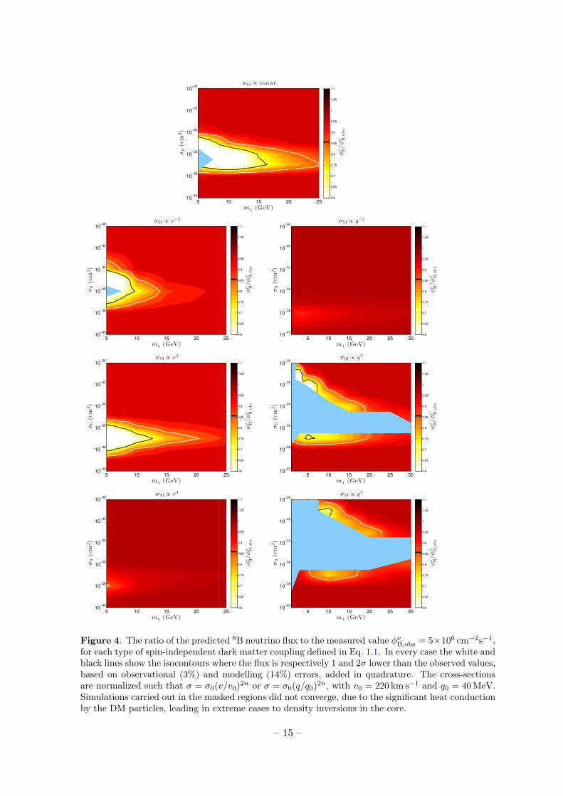
Figure 4. The ratio of the predicted 8B neutrino flux to the measured value φνB,obs = 5×106 cm−2s−1,for each type of spin-independent dark matter coupling defined in Eq. 1.1. In every case the white andblack lines show the isocontours where the flux is respectively 1 and 2σ lower than the observed values,based on observational (3%) and modelling (14%) errors, added in quadrature. The cross-sectionsare normalized such that σ = σ0(v/v0)2n or σ = σ0(q/q0)2n, with v0 = 220 km s−1 and q0 = 40 MeV.Simulations carried out in the masked regions did not converge, due to the significant heat conductionby the DM particles, leading in extreme cases to density inversions in the core.

– 15 –

σ0(cm

2)

mχ (GeV)

σSD ∝ const.

5 10 15 20 2510

−40

10−38

10−36

10−34

10−32

φν B/φν B,obs

0.6

0.65

0.7

0.75

0.8

0.85

0.9

0.95

1

1.05

1.1

σ0(cm

2)

mχ (GeV)

σSD ∝ v−2

5 10 15 20 25 3010

−40

10−38

10−36

10−34

10−32

10−30

φν B/φν B,obs

0.6

0.65

0.7

0.75

0.8

0.85

0.9

0.95

1

1.05

1.1

σ0(cm

2)

mχ (GeV)

σSD ∝ q−2

5 10 15 20 2510

−40

10−38

10−36

10−34

10−32

10−30

φν B/φν B,obs

0.6

0.65

0.7

0.75

0.8

0.85

0.9

0.95

1

1.05

1.1

σ0(cm

2)

mχ (GeV)

σSD ∝ v2

5 10 15 20 2510

−40

10−38

10−36

10−34

10−32

10−30

φν B/φν B,obs

0.6

0.65

0.7

0.75

0.8

0.85

0.9

0.95

1

1.05

1.1

σ0(cm

2)

mχ (GeV)

σSD ∝ q2

5 10 15 20 2510

−40

10−38

10−36

10−34

10−32

10−30

φν B/φν B,obs

0.6

0.65

0.7

0.75

0.8

0.85

0.9

0.95

1

1.05

1.1

σ0(cm

2)

mχ (GeV)

σSD ∝ v4

5 10 15 20 2510

−40

10−38

10−36

10−34

10−32

10−30

φν B/φν B,obs

0.6

0.65

0.7

0.75

0.8

0.85

0.9

0.95

1

1.05

1.1

σ0(cm

2)

mχ (GeV)

σSD ∝ q4

5 10 15 20 2510

−40

10−38

10−36

10−34

10−32

10−30

φν B/φν B,obs

0.6

0.65

0.7

0.75

0.8

0.85

0.9

0.95

1

1.05

1.1

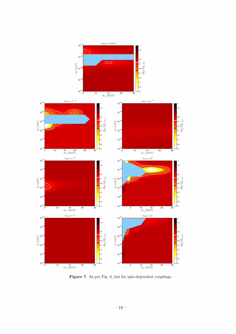
Figure 5. As per Fig. 4, but for spin-dependent couplings.

– 16 –

σ0(cm

2)

mχ (GeV)

σSI ∝ const.

5 10 15 20 2510

−40

10−38

10−36

10−34

10−32

10−30

φν Be/φν Be,obs

0.6

0.65

0.7

0.75

0.8

0.85

0.9

0.95

1

1.05

1.1σ0(cm

2)

mχ (GeV)

σSI ∝ v−2

5 10 15 20 2510

−40

10−38

10−36

10−34

10−32

10−30

φν Be/φν Be,obs

0.6

0.65

0.7

0.75

0.8

0.85

0.9

0.95

1

1.05

1.1

σ0(cm

2)

mχ (GeV)

σSI ∝ q−2

5 10 15 20 25 3010

−40

10−38

10−36

10−34

10−32

10−30

φν Be/φν Be,obs

0.6

0.65

0.7

0.75

0.8

0.85

0.9

0.95

1

1.05

1.1

σ0(cm

2)

mχ (GeV)

σSI ∝ v2

5 10 15 20 2510

−40

10−38

10−36

10−34

10−32

10−30

φν Be/φν Be,obs

0.6

0.65

0.7

0.75

0.8

0.85

0.9

0.95

1

1.05

1.1

σ0(cm

2)

mχ (GeV)

σSI ∝ q2

5 10 15 20 25 3010

−40

10−38

10−36

10−34

10−32

10−30

φν Be/φν Be,obs

0.6

0.65

0.7

0.75

0.8

0.85

0.9

0.95

1

1.05

1.1

σ0(cm

2)

mχ (GeV)

σSI ∝ v4

5 10 15 20 2510

−40

10−38

10−36

10−34

10−32

10−30

φν Be/φν Be,obs

0.6

0.65

0.7

0.75

0.8

0.85

0.9

0.95

1

1.05

1.1

σ0(cm

2)

mχ (GeV)

σSI ∝ q4

5 10 15 20 25 3010

−40

10−38

10−36

10−34

10−32

10−30

φν Be/φν Be,obs

0.6

0.65

0.7

0.75

0.8

0.85

0.9

0.95

1

1.05

1.1

Figure 6. The ratio of the predicted 7Be neutrino flux to the measured value φνBe,obs = 4.82 ×109 cm−2s−1, for each type of spin-independent dark matter coupling defined in Eq. 1.1. In every casethe white and black lines show the isocontours where the flux is respectively 1 and 2σ lower than theobserved values, based on observational (5%) and modelling (7%) errors, added in quadrature. Thecross-sections are normalized such that σ = σ0(v/v0)2n or σ = σ0(q/q0)2n, with v0 = 220 km s−1 andq0 = 40 MeV.

– 17 –

σ0(cm

2)

mχ (GeV)

σSD ∝ const.

5 10 15 20 2510

−40

10−38

10−36

10−34

10−32

φν Be/φν Be,obs

0.6

0.65

0.7

0.75

0.8

0.85

0.9

0.95

1

1.05

1.1

σ0(cm

2)

mχ (GeV)

σSD ∝ v−2

5 10 15 20 25 3010

−40

10−38

10−36

10−34

10−32

10−30

φν Be/φν Be,obs

0.6

0.65

0.7

0.75

0.8

0.85

0.9

0.95

1

1.05

1.1

σ0(cm

2)

mχ (GeV)

σSD ∝ q−2

5 10 15 20 2510

−40

10−38

10−36

10−34

10−32

10−30

φν Be/φν Be,obs

0.6

0.65

0.7

0.75

0.8

0.85

0.9

0.95

1

1.05

1.1

σ0(cm

2)

mχ (GeV)

σSD ∝ v2

5 10 15 20 2510

−40

10−38

10−36

10−34

10−32

10−30

φν Be/φν Be,obs

0.6

0.65

0.7

0.75

0.8

0.85

0.9

0.95

1

1.05

1.1

σ0(cm

2)

mχ (GeV)

σSD ∝ q2

5 10 15 20 2510

−40

10−38

10−36

10−34

10−32

10−30

φν Be/φν Be,obs

0.6

0.65

0.7

0.75

0.8

0.85

0.9

0.95

1

1.05

1.1

σ0(cm

2)

mχ (GeV)

σSD ∝ v4

5 10 15 20 2510

−40

10−38

10−36

10−34

10−32

10−30

φν Be/φν Be,obs

0.6

0.65

0.7

0.75

0.8

0.85

0.9

0.95

1

1.05

1.1

σ0(cm

2)

mχ (GeV)

σSD ∝ q4

5 10 15 20 2510

−40

10−38

10−36

10−34

10−32

10−30

φν Be/φν Be,obs

0.6

0.65

0.7

0.75

0.8

0.85

0.9

0.95

1

1.05

1.1

Figure 7. As per Fig. 6, but for spin-dependent couplings.

– 18 –

As expected, the effect of ADM on neutrino fluxes is larger for low DM masses, mainlydue to the increased efficiency of momentum transfer between DM and H/He as the DM takeson a similar mass to these two dominant nuclei. Ignoring evaporation, transport becomeseven more efficient as mass is decreased to 1 GeV for SD dark matter; in the SI case, thelargest effect is seen at mχ ' 3 to 4 GeV, around the average nucleus mass in the Sun.

The dependence on the cross-section is also as expected: below a minimum value ofσ0, not enough DM can be captured to significantly affect the 8B production rate. Forconstant cross-sections, this is around 10−38 cm2 in the SI case, and 10−36 cm2 for SD darkmatter. This highlights the importance of heavier elements, to which only the SI DM couplesin our simulations: the large fraction of helium, combined with the A2 dependence of theDM-nucleus cross-section (Eq. 1.2) means that the behaviour of DM inside a star is highlysensitive to elements heavier than hydrogen.

The upper edges of the regions shown in Figs. 4–7 highlight the transport behaviour: ifthe cross-section falls below a certain value, it allows the DM to more efficiently penetratethe dense plasma, carrying energy from hot to cooler regions. The location of the maximumreflects a combination of being near the transport efficiency peak (where the transition fromthe LTE to the Knudsen regime occurs) while simultaneously maintaining a large capturerate through a large enough cross-section.

The impacts of velocity and momentum-dependent scattering of dark matter can beunderstood in terms of this balance between capture and transport. Positive powers of vrellead to an enhancement in the capture rate, moving the window in which DM transporthas a significant effect on neutrino fluxes to lower cross-sections. However, the importantsuppression in the overall transport rate, as seen in Fig. 5 of [88], yields an overall suppressionin the effect relative to the constant case. The opposite behaviour is seen for σ ∝ v−2rel ,although the enhanced transport is not sufficient to compensate for the ∼10−2 suppressionin capture.

Again, the effect of a momentum-dependent cross-section is more subtle. Althoughthe boosted capture rate for a q−2 cross-section moves the region of interest to lower cross-sections, closer to what is allowed by underground experiments, the overall suppression intransport means that there is very little overall effect on solar observables. Positive powersof q fare much better, with an enhancement both in capture and transport.

Comparison of Figs. 4 and 5 highlights the importance of heavier elements in suchprocesses. In most cases, they lead to a significant enhancement of the capture and transportrate; however, we note in comparing the q−2 plots that they can also inhibit energy transport,by reducing the mean free path for conduction.

5.3 Depth of the convection zone

The boundary between the convective and radiative zones rCZ is the location at which the ra-diative and adiabatic temperature gradients are equal. Above this location, the temperaturegradient becomes super-adiabatic, hydrostatic equilibrium breaks down and convection setsin. The amount of energy transported by DM is negligible at heights r ∼ rCZ. However, thechanges in the density and temperature gradient near the core lead to a small but significantincrease in the radiative temperature gradient at much larger radii, causing it to exceed theadiabatic gradient at a slightly lower depth and shift the lower boundary of the convectionzone downwards.

In Figs. 8 and 9, we show the ratio of the location of the lower boundary of the convectionzone predicted by each model to the value inferred from helioseismology, rCZ, = 0.713R.

– 19 –

σ0(cm

2)

mχ (GeV)

σSI ∝ const.

5 10 15 20 2510

−40

10−38

10−36

10−34

10−32

10−30

rCZ/rCZ,⊙

1

1.002

1.004

1.006

1.008

1.01

1.012

σ0(cm

2)

mχ (GeV)

σSI ∝ v−2

5 10 15 20 2510

−40

10−38

10−36

10−34

10−32

10−30

rCZ/rCZ,⊙

1

1.002

1.004

1.006

1.008

1.01

1.012

σ0(cm

2)

mχ (GeV)

σSI ∝ q−2

5 10 15 20 25 3010

−40

10−38

10−36

10−34

10−32

10−30

rCZ/rCZ,⊙

1

1.002

1.004

1.006

1.008

1.01

1.012

σ0(cm

2)

mχ (GeV)

σSI ∝ v2

5 10 15 20 2510

−40

10−38

10−36

10−34

10−32

10−30

rCZ/rCZ,⊙

1

1.002

1.004

1.006

1.008

1.01

1.012

σ0(cm

2)

mχ (GeV)

σSI ∝ q2

5 10 15 20 25 3010

−40

10−38

10−36

10−34

10−32

10−30

rCZ/rCZ,⊙

1

1.002

1.004

1.006

1.008

1.01

1.012

σ0(cm

2)

mχ (GeV)

σSI ∝ v4

5 10 15 20 2510

−40

10−38

10−36

10−34

10−32

10−30

rCZ/rCZ,⊙

1

1.002

1.004

1.006

1.008

1.01

1.012

σ0(cm

2)

mχ (GeV)

σSI ∝ q4

5 10 15 20 25 3010

−40

10−38

10−36

10−34

10−32

10−30

rCZ/rCZ,⊙

1

1.002

1.004

1.006

1.008

1.01

1.012

Figure 8. Ratio between the modelled and measured location of the bottom of the convection zonerCZ, for spin-independent couplings. Darker regions represent a better fit to the observed value thanthe Standard Solar Model. The white and black lines represent the contours at which the predictedvalue falls within 1σ and 2σ of the measured value, respectively. The theoretical uncertainty on rCZ

(0.004R) is much larger than the experimental error (0.001R), so the former dominates when weadd them in quadrature.

– 20 –

σ0(cm

2)

mχ (GeV)

σSD ∝ const.

5 10 15 20 2510

−40

10−38

10−36

10−34

10−32

rCZ/rCZ,⊙

1

1.002

1.004

1.006

1.008

1.01

1.012

σ0(cm

2)

mχ (GeV)

σSD ∝ v−2

5 10 15 20 25 3010

−40

10−38

10−36

10−34

10−32

10−30

rCZ/rCZ,⊙

1

1.002

1.004

1.006

1.008

1.01

1.012

σ0(cm

2)

mχ (GeV)

σSD ∝ q−2

5 10 15 20 2510

−40

10−38

10−36

10−34

10−32

10−30

rCZ/rCZ,⊙

1

1.002

1.004

1.006

1.008

1.01

1.012

σ0(cm

2)

mχ (GeV)

σSD ∝ v2

5 10 15 20 2510

−40

10−38

10−36

10−34

10−32

10−30

rCZ/rCZ,⊙

1

1.002

1.004

1.006

1.008

1.01

1.012

σ0(cm

2)

mχ (GeV)

σSD ∝ q2

5 10 15 20 2510

−40

10−38

10−36

10−34

10−32

10−30

rCZ/rCZ,⊙

1

1.002

1.004

1.006

1.008

1.01

1.012

σ0(cm

2)

mχ (GeV)

σSD ∝ v4

5 10 15 20 2510

−40

10−38

10−36

10−34

10−32

10−30

rCZ/rCZ,⊙

1

1.002

1.004

1.006

1.008

1.01

1.012

σ0(cm

2)

mχ (GeV)

σSD ∝ q4

5 10 15 20 2510

−40

10−38

10−36

10−34

10−32

10−30

rCZ/rCZ,⊙

1

1.002

1.004

1.006

1.008

1.01

1.012

Figure 9. As per Fig. 8, but for spin-dependent couplings.

– 21 –

Although the error on the helioseismological inference is just 0.001R, the theoretical error onthe modelled rCZ, is much larger: σCZ,,th = 0.004R. Adding these errors in quadrature,we plot in white and black the contours containing the regions where rCZ, is within 1σ and2σ, respectively, of the inferred value.

As can be seen in Figs. 8 and 9, the difference between the depth of the convection zonein the Standard Solar Model (rCZ, = 0.722R) and the depth inferred from helioseismologyamounts to almost a 3σ discrepancy. Except for a small region at high q2 cross-section(σ0 = 10−33 cm2), spin-dependent DM struggles to bring rCZ to within much better than 2σof the inferred value. However, energy conduction from SI interactions does substantiallybetter: v±2rel and q2 models can produce good agreement with the observed value of rCZ,,leading in some regions to agreement at better than 1σ.

5.4 Surface helium abundance

The surface helium abundance Ys is another observable that has fallen into disagreement withobservations since the revision of the solar composition. Our SSM prediction is Ys = 0.2356,whereas the observed value is 0.2485 ±0.0034. With theoretical errors of ±0.0035 takeninto account, this amounts to a discrepancy of 3σ. The addition of dark matter does verylittle to change Ys, and for most models the discrepancy remains at the 3σ level. For somevery few cases (not shown), it actually worsens the discrepancy by up to an additional ∼2σ.This only occurs for models where the fit to sound speed observables is also substantiallyworsened, notably for large SD q2 and q4 cross-sections. The reduction in Ys is caused by acorresponding increase in Xi, the initial hydrogen fraction. The increase in Xi is demandedby the reduction of the core temperature, which requires a greater amount of hydrogen to bepresent in the core in order to maintain the same nuclear burning rate as in the SSM, andto thereby match the observed solar luminosity L.

Because it changes little, we do not show the contour plots for the surface He abundance.For completeness though, we include it anyway in our full likelihood computation in Sec. 5.7.

5.5 Sound speed profile

In Fig. 10 we show the deviation of the modelled radial sound speed of some models thatproduced the best overall fits with respect to the measured values from helioseismology. Toillustrate the agreement of each model with the observed sound speed profile, we constructan effective chi-squared measure

χ2cs =

∑ri

[cs,model(ri)− cs,hel.(ri)]2

σ2cs,hel.(ri)(5.1)

where the sum goes over 5 equally-spaced radial points between r = 0.1R and 0.67R. Wedo not include radii below 0.1R because the reconstructed sound speed in this region ishighly uncertain due to the low number of low-degree (low-l) p-modes reaching the innermostradii of the solar core [110]. The upper limit of the range is the location of the largestdiscrepancy in the sound speed of the Standard Solar Model, at the base of the convectionzone; above this point essentially all models agree very well with the observed sound speedbecause the temperature gradient is adiabatic and therefore does not depend on the detailedcomposition of the Sun. We added errors from modelling and inversions for each point inquadrature. We obtained modelling errors by using models for which one input parameterwas varied at a time to obtain partial derivatives at each radial point, and then combined

– 22 –

0.1 0.2 0.3 0.4 0.5 0.6 0.7 0.8 0.9−6

−4

−2

0

2

4

6

8

10x 10

−3

R/R⊙

δc s/c s

Modelling errorHeliose ismology errorNo DMmχ = 15 GeV,σS I = 10−37 cm2

mχ = 5 GeV,σSD = 10−33 cm2

0.1 0.2 0.3 0.4 0.5 0.6 0.7 0.8 0.9−6

−4

−2

0

2

4

6

8

10x 10

−3

R/R⊙

δc s/c s

Modelling errorHeliose ismology errorNo DMq 2,SDq 2,SIv 2,SI

Figure 10. Deviation of radial sound speed profile from values inferred from helioseismology. Left:the best overall fits with constant spin-dependent (SD) and spin-independent (SI) cross-sections.Right: best-fit models of the three couplings returning the best overall p-values (see Tab. 1): (q2,SD): mχ = 5 GeV, σ0 = 10−30 cm2; (q2, SI): mχ = 3 GeV, σ0 = 10−37 cm2; and (v2, SI): mχ = 5GeV, σ0 = 10−35 cm2.

quadratically given the uncertainty in the AGSS09 abundances and errors in each parameterquoted in [111]. The errors on inversions were taken from [112]. The values of this χ2, meantto show the relative improvement to the sound speed modelling, are shown in Figs. 11 and12.

From these figures, along with the sound speed profiles illustrated in Fig. 10, it is clearthat the addition of momentum or velocity-dependent dark matter to the solar model doesindeed help alleviate the discrepancy between modelling and observation in some specificcases. We will return to these cases in Sec. 6.1.

5.6 Frequency separation ratios

The inverted sound speed profile cs(r) obtained from helioseismological measurements is notvery accurate near the solar core because not enough low-l p-modes are available for a preciseand accurate inversion. Instead, information about the solar core can be gained by using theso-called frequency separation ratios. A large advantage of using these ratios is that, unlikeindividual frequencies, they are not affected by the detailed structure of the solar surface,which is poorly described by solar models [113]. This is because for radial order n 1 andlow angular degree l, the surface effects are functions of the eigenfrequency, so they cancel outwhen considering frequency differences between modes of similar frequencies. In addition,by taking ratios of appropriate frequency differences, the solar core structure becomes thedominant effect in the observed signal [114, 115]. In particular, two very useful quantitiesare the frequency separation ratios

r02(n) =d02(n)

∆1(n), r13(n) =

d13(n)

∆0(n+ 1), (5.2)

where

dl,l+2(n) ≡ νn,l − νn−1,l+2 ' −(4l + 6)∆l(n)

4π2νn,l

∫ R

0

dcsdr

dr

r. (5.3)

– 23 –

σ0(cm

2)

mχ (GeV)

σSI ∝ const.

5 10 15 20 2510

−40

10−38

10−36

10−34

10−32

10−30

χ2

0

5

10

15

20

25

30

35

40

45

50

σ0(cm

2)

mχ (GeV)

σSI ∝ v−2

5 10 15 20 2510

−40

10−38

10−36

10−34

10−32

10−30

χ2

0

5

10

15

20

25

30

35

40

45

50

σ0(cm

2)

mχ (GeV)

σSI ∝ q−2

5 10 15 20 25 3010

−40

10−38

10−36

10−34

10−32

10−30

χ2

0

5

10

15

20

25

30

35

40

45

50

σ0(cm

2)

mχ (GeV)

σSI ∝ v2

5 10 15 20 2510

−40

10−38

10−36

10−34

10−32

10−30

χ2

0

5

10

15

20

25

30

35

40

45

50

σ0(cm

2)

mχ (GeV)

σSI ∝ q2

5 10 15 20 25 3010

−40

10−38

10−36

10−34

10−32

10−30

χ2

0

5

10

15

20

25

30

35

40

45

50

σ0(cm

2)

mχ (GeV)

σSI ∝ v4

5 10 15 20 2510

−40

10−38

10−36

10−34

10−32

10−30

χ2

0

5

10

15

20

25

30

35

40

45

50

σ0(cm

2)

mχ (GeV)

σSI ∝ q4

5 10 15 20 25 3010

−40

10−38

10−36

10−34

10−32

10−30

χ2

0

5

10

15

20

25

30

35

40

45

50

Figure 11. Effective sound-speed χ2cs defined in Eq. 5.1, showing the improvement in goodness-of-fit

of the radial sound speed profile in solar models with different types of spin-independent ADM. Theχ2 value of the best fit point is indicated by a green line on the colour bar and is shown as a greenstar in each figure. ∆χ2 = 2.3 and 6.18 contours, corresponding to 1σ and 2σ deviations from thebest fit, are respectively shown in white and black.

– 24 –

σ0(cm

2)

mχ (GeV)

σSD ∝ const.

5 10 15 20 2510

−40

10−38

10−36

10−34

10−32

χ2

0

5

10

15

20

25

30

35

40

45

50

σ0(cm

2)

mχ (GeV)

σSD ∝ v−2

5 10 15 20 25 3010

−40

10−38

10−36

10−34

10−32

10−30

χ2

0

5

10

15

20

25

30

35

40

45

50

σ0(cm

2)

mχ (GeV)

σSD ∝ q−2

5 10 15 20 2510

−40

10−38

10−36

10−34

10−32

10−30

χ2

0

5

10

15

20

25

30

35

40

45

50

σ0(cm

2)

mχ (GeV)

σSD ∝ v2

5 10 15 20 2510

−40

10−38

10−36

10−34

10−32

10−30

χ2

0

5

10

15

20

25

30

35

40

45

50

σ0(cm

2)

mχ (GeV)

σSD ∝ q2

5 10 15 20 2510

−40

10−38

10−36

10−34

10−32

10−30

χ2

0

5

10

15

20

25

30

35

40

45

50

σ0(cm

2)

mχ (GeV)

σSD ∝ v4

5 10 15 20 2510

−40

10−38

10−36

10−34

10−32

10−30

χ2

0

5

10

15

20

25

30

35

40

45

50

σ0(cm

2)

mχ (GeV)

σSD ∝ q4

5 10 15 20 2510

−40

10−38

10−36

10−34

10−32

10−30

χ2

0

5

10

15

20

25

30

35

40

45

50

Figure 12. Same as Fig. 11, but for spin-dependent couplings.

– 25 –

1000 1500 2000 2500 3000 3500 40000.055

0.06

0.065

0.07

0.075

0.08

0.085

0.09

0.095r 0

2

BiSON dataStandard solar modelmχ = 15 GeV, σSI = 10−37 cm2

mχ = 5 GeV, σSD = 10−33 cm2

ν (µHz)

(rmod−

r obs)/σobs

1000 1500 2000 2500 3000 3500 4000

−4

−2

0

2

4

1000 1500 2000 2500 3000 3500 40000.055

0.06

0.065

0.07

0.075

0.08

0.085

0.09

0.095

r 02

BiSON dataStandard solar modelSD, q2, mχ = 5 GeV, σ0 = 10−30 cm2

SI, q2, mχ = 3 GeV, σ0 = 10−37 cm2

SD, v2, mχ = 5 GeV, σ0 = 10−35 cm2

ν (µHz)

(rmod−

r obs)/σobs

1000 1500 2000 2500 3000 3500 4000

−4

−2

0

2

4

1000 1500 2000 2500 3000 3500 40000.1

0.11

0.12

0.13

0.14

0.15

0.16

r13

BiSON dataStandard solar modelmχ = 15 GeV, σSI = 10−37 cm2

mχ = 5 GeV, σSD = 10−33 cm2

ν (µHz)

(rmod−

r obs)/σobs

1000 1500 2000 2500 3000 3500 4000

−4

−2

0

2

4

1000 1500 2000 2500 3000 3500 40000.1

0.11

0.12

0.13

0.14

0.15

0.16

r13

BiSON dataStandard solar modelSD, q2, mχ = 5 GeV, σ0 = 10−30 cm2

SI, q2, mχ = 3 GeV, σ0 = 10−37 cm2

SD, v2, mχ = 5 GeV, σ0 = 10−35 cm2

ν (µHz)

(rmod−

r obs)/σobs

1000 1500 2000 2500 3000 3500 4000

−4

−2

0

2

4

Figure 13. Small frequency separations r02 (top) and r13 (bottom) as defined in Eq. 5.2, for the bestfit constant (left) and generalised form-factor dark matter models (right). The latter correspond tothe best-fit models of the three couplings returning the best overall p-values (see Tab. 1). Predictionsare compared with helioseismological observations from the BiSON experiment [114]. Inner blackerror bars correspond to observational error, whereas outer (green) bars also include modelling error.Below each figure we show the residuals with respect to BiSON data, in units of the total error.The mχ = 3 GeV, q2 case with σ0 = 10−37 cm2 yields the best improvement, bringing the largestdiscrepancy from nearly 4σ to little more than a standard deviation.

– 26 –

and ∆l(n) ≡ νn,l−νn−1,l. The sound speed gradient is weighted by 1/r in the integral above,so r02(n) and r13(n) are most sensitive to changes there.

We show a set of these ratios in Fig. 13 for the same examples shown in Fig. 10. Theseare compared with the values of r02(n) and r13(n) measured by the BiSON experiment [115].Model uncertainties are computed following the same procedure as for the sound speed. Ascan be seen in the residual subplots, the SSM overestimates each of these ratios by as much as4σ, once modelling errors are included. Thermal transport by ADM can smooth the soundspeed gradient, yielding smaller differences in Eq. 5.3. As in the case of the sound speedprofile, the best improvement is provided by q2 scattering with mχ = 3 GeV, σ0 = 10−37

cm2. In this model, the largest discrepancy in r02 and r13 falls to barely 1σ.In Figs. 14 and 15, we show the overall ability of different models to fit the observed

frequency separations. We quantify this with the combined chi-squared χ2r02 + χ2

r13 , where

χ2r`,`+2

=∑n

[r`,`+2,th.(n)− r`,`+2,obs.(n)]2

σ2obs.(n) + σ2th.(n). (5.4)

Formally, there is a correlation between values of r02(n) and r13(n) with common eigenfre-quencies. In practice, however, the correlation is minimal (the Pearson correlation coefficientis always lower than 0.1), so we assume they are independent when computing χ2

r02 + χ2r13 .

Figs. 14 and 15 show that all SI and SD couplings do exhibit areas of parameter space wherethe small frequency separations can be brought into better agreement with observations thanin the SSM. In many cases however, these are not the same parameter combinations preferredby other observables. The notable exception to this is the q2 SI coupling, which also clearlyproduces the best agreement with the observed frequency separations.

5.7 Combined limits

It is clear from the results we have presented in Secs. 5.2–5.6 that the disagreement betweenmodel predictions and helioseismology can be ameliorated, at the cost of a slightly worseagreement with neutrino fluxes. Surface helium Ys is also affected to a lesser extent. It istherefore instructive to construct an overall likelihood function based on the fit of these databy our models. We define the combined chi-squared as:

χ2 =(1− φνB,obs/φνB)2

σ2B+

(1− φνBe,obs/φνBe)

2

σ2Be

+(rCZ − rCZ,obs)

2

σ2CZ

+(YS − YS,obs)2

σ2YS+χ2

r02 + χ2r13 . (5.5)

where φνB,obs = 5.00 × 106 cm−2s−1, φνBe,obs = 4.82 × 109cm−2s−1, rCZ,obs = 0.713R andYS,obs = 0.2485. The uncertainties include both the observational and modelling errors,added in quadrature. These are given individually in the last two lines of Table 1. Weinclude the small frequency separations r`,`+2, but not the sound speed profile, as the latteris less precise and is correlated with the former.

We show the combined limits from Eq. 5.5 in Figs. 16 and 17, comparing with limitsfrom direct detection where such results exist (i.e. in the SI case; [30]). We discuss theseresults, and the comparison with other limits, in more detail in the following section.

– 27 –

σ0(cm

2)

mχ (GeV)

σSI ∝ const.

5 10 15 20 2510

−40

10−38

10−36

10−34

10−32

10−30

χ2 r02+

χ2 r13

0

50

100

150

200

250

300

σ0(cm

2)

mχ (GeV)

σSI ∝ v−2

5 10 15 20 2510

−40

10−38

10−36

10−34

10−32

10−30

χ2 r02+

χ2 r13

0

50

100

150

200

250

300

σ0(cm

2)

mχ (GeV)

σSI ∝ q−2

5 10 15 20 25 3010

−40

10−38

10−36

10−34

10−32

10−30

χ2 r02+

χ2 r13

0

50

100

150

200

250

300

σ0(cm

2)

mχ (GeV)

σSI ∝ v2

5 10 15 20 2510

−40

10−38

10−36

10−34

10−32

10−30

χ2 r02+

χ2 r13

0

50

100

150

200

250

300

σ0(cm

2)

mχ (GeV)

σSI ∝ q2

5 10 15 20 25 3010

−40

10−38

10−36

10−34

10−32

10−30

χ2 r02+

χ2 r13

0

50

100

150

200

250

300

σ0(cm

2)

mχ (GeV)

σSI ∝ v4

5 10 15 20 2510

−40

10−38

10−36

10−34

10−32

10−30

χ2 r02+

χ2 r13

0

50

100

150

200

250

300

σ0(cm

2)

mχ (GeV)

σSI ∝ q4

5 10 15 20 25 3010

−40

10−38

10−36

10−34

10−32

10−30

χ2 r02+

χ2 r13

0

50

100

150

200

250

300

Figure 14. Combined likelihood χ2r02 + χ2

r13 for the small frequency separations defined in Eq. 5.2,for different models of ADM with spin-independent scattering cross sections. The green line on thecolour bar shows the χ2 value of the best fit, indicated by a green star in each panel, whereas white,black and cyan lines show the preferred regions at 1, 2 and 4 σ confidence levels, respectively. Atlow masses, many DM models can yield improvements in the overall chi-squared with respect to theStandard Solar Model, but the q2 model provides a clear best fit.

– 28 –

σ0(cm

2)

mχ (GeV)

σSD ∝ const.

5 10 15 20 2510

−40

10−38

10−36

10−34

10−32

χ2 r02+

χ2 r13

0

50

100

150

200

250

300

σ0(cm

2)

mχ (GeV)

σSD ∝ v−2

5 10 15 20 25 3010

−40

10−38

10−36

10−34

10−32

10−30

χ2 r02+

χ2 r13

0

50

100

150

200

250

300

σ0(cm

2)

mχ (GeV)

σSD ∝ q−2

5 10 15 20 2510

−40

10−38

10−36

10−34

10−32

10−30

χ2 r02+

χ2 r13

0

50

100

150

200

250

300

σ0(cm

2)

mχ (GeV)

σSD ∝ v2

5 10 15 20 2510

−40

10−38

10−36

10−34

10−32

10−30

χ2 r02+

χ2 r13

0

50

100

150

200

250

300

σ0(cm

2)

mχ (GeV)

σSD ∝ q2

5 10 15 20 2510

−40

10−38

10−36

10−34

10−32

10−30

χ2 r02+

χ2 r13

0

50

100

150

200

250

300

σ0(cm

2)

mχ (GeV)

σSD ∝ v4

5 10 15 20 2510

−40

10−38

10−36

10−34

10−32

10−30

χ2 r02+

χ2 r13

0

50

100

150

200

250

300

σ0(cm

2)

mχ (GeV)

σSD ∝ q4

5 10 15 20 2510

−40

10−38

10−36

10−34

10−32

10−30

χ2 r02+

χ2 r13

0

50

100

150

200

250

300

Figure 15. Same as Fig. 14, but for spin-dependent couplings.

– 29 –

σ0(cm

2)

mχ (GeV)

σSI ∝ const.

5 10 15 20 2510

−40

10−38

10−36

10−34

10−32

10−30

χ2

0

50

100

150

200

250

300

σ0(cm

2)

mχ (GeV)

σSI ∝ v−2

5 10 15 20 2510

−40

10−38

10−36

10−34

10−32

10−30

χ2

0

50

100

150

200

250

300

σ0(cm

2)

mχ (GeV)

σSI ∝ q−2

5 10 15 20 25 3010

−40

10−38

10−36

10−34

10−32

10−30

χ2

0

50

100

150

200

250

300

σ0(cm

2)

mχ (GeV)

σSI ∝ v2

5 10 15 20 2510

−40

10−38

10−36

10−34

10−32

10−30

χ2

0

50

100

150

200

250

300

σ0(cm

2)

mχ (GeV)

σSI ∝ q2

5 10 15 20 25 3010

−40

10−38

10−36

10−34

10−32

10−30

χ2

0

50

100

150

200

250

300

σ0(cm

2)

mχ (GeV)

σSI ∝ v4

5 10 15 20 2510

−40

10−38

10−36

10−34

10−32

10−30

χ2

0

50

100

150

200

250

300

σ0(cm

2)

mχ (GeV)

σSI ∝ q4

5 10 15 20 25 3010

−40

10−38

10−36

10−34

10−32

10−30

χ2

0

50

100

150

200

250

300

Figure 16. Full combined likelihood (Eq. 5.5) incorporating 8B and 7Be neutrino flux measurements,the surface helium abundance YS, the radius of the convection zone and the small frequency separa-tions. The χ2 value of the best fit point is shown as a green star, and indicated by a green line on thecolour bar. ∆χ2 = 2.3, 6.18 and 19.33 contours corresponding to 1σ, 2σ and 4σ deviations from thebest fit are shown in white, black and cyan, respectively.

– 30 –

σ0(cm

2)

mχ (GeV)

σSD ∝ const.

5 10 15 20 2510

−40

10−38

10−36

10−34

10−32

χ2

0

50

100

150

200

250

300

σ0(cm

2)

mχ (GeV)

σSD ∝ v−2

5 10 15 20 25 3010

−40

10−38

10−36

10−34

10−32

10−30

χ2

0

50

100

150

200

250

300

σ0(cm

2)

mχ (GeV)

σSD ∝ q−2

5 10 15 20 2510

−40

10−38

10−36

10−34

10−32

10−30

χ2

0

50

100

150

200

250

300

σ0(cm

2)

mχ (GeV)

σSD ∝ v2

5 10 15 20 2510

−40

10−38

10−36

10−34

10−32

10−30

χ2

0

50

100

150

200

250

300

σ0(cm

2)

mχ (GeV)

σSD ∝ q2

5 10 15 20 2510

−40

10−38

10−36

10−34

10−32

10−30

χ2

0

50

100

150

200

250

300

σ0(cm

2)

mχ (GeV)

σSD ∝ v4

5 10 15 20 2510

−40

10−38

10−36

10−34

10−32

10−30

χ2

0

50

100

150

200

250

300

σ0(cm

2)

mχ (GeV)

σSD ∝ q4

5 10 15 20 2510

−40

10−38

10−36

10−34

10−32

10−30

χ2

0

50

100

150

200

250

300

Figure 17. Same as Fig. 16, but for spin-dependent couplings.

– 31 –

Table 1. Standard Solar Model (SSM) and best fit (b.f.) values for each of the models we consider,along with observable quantities. The DM mass and cross-sections are in GeV and cm2, respectively.The boron-8 neutrino flux φνB is in units of 10−6 cm−2 s−1 and the beryllium-7 neutrino flux φνBe

is expressed in 10−9 cm−2 s−1. The full chi-squared is defined in Eq. 5.5 and includes the neutrinofluxes, surface helium abundance YS , depth of the convection zone and small frequency separations.

Model (mχ, σ0)b.f. φνB φνBe RCZ/R Ys χ2 p

SSM – 4.95 4.71 0.722 0.2356 287.8 < 10−10

σSI

const. (15,10−37) 3.48 4.37 0.721 0.2348 122.2 < 10−10

q−2 (3,10−38) 4.51 4.59 0.721 0.2350 144.1 < 10−10

q2 (3, 10−37) 3.78 4.29 0.718 0.2327 27.5 0.85q4 (10, 10−31) 3.29 4.27 0.721 0.2348 98.2 1.1× 10−7

v−2 (5,10−34) 3.91 4.44 0.721 0.2347 86.4 5.0× 10−6

v2 (5, 10−38) 3.31 4.22 0.719 0.2337 135.0 < 10−10

v4 (5,10−38) 4.30 4.54 0.721 0.2349 114.9 3.6× 10−10

σSD

const. (5,10−33) 3.36 4.27 0.720 0.2341 100.2 5.8× 10−8

q−2 (5,10−38) 4.43 4.59 0.722 0.2353 174.5 < 10−10

q2 (5,10−30) 3.64 4.35 0.720 0.2343 73.1 2.5× 10−4

q4 (15,10−30) 3.81 4.47 0.721 0.2351 140.7 < 10−10

v−2 (10,10−32) 3.39 4.33 0.721 0.2347 114.5 4.2× 10−10

v2 (5,10−35) 3.75 4.39 0.721 0.2344 72.4 3.1× 10−4

v4 (5,10−37) 4.80 4.68 0.722 0.2355 238.7 < 10−10

Obs. – 5.00 4.82 0.713 0.2485 – –

Obs. error – 3 % 5% 0.001 0.0034 – –Model error – 14 % 7% 0.004 0.0035 – –

In Table 1, we give a break-down of the values of each observable at the best-fit parame-ters of each model, along with the best-fit χ2 and implied p-value. The best-fit regular SI andSD cases shown in Table 1 differ from the best-fit cases in Ref. [72] because here we actuallychoose them on the basis of the full likelihood Eq. 5.5. In Ref. [72] we only computed thesmall-frequency separations for models that provided the best fits to all other observables.Because the fits to different observables are inconsistent in the models with constant cross-sections, including the frequency separations shifts the best-fit masses and cross-sections.This is to be compared to the q2 SI case, where adding in the small frequencies merely makesthe best-fit point even better.

We also provide as supplementary material online a complete table of the boron andberyllium neutrino fluxes, surface helium, convective zone radius and small frequency sepa-rations for all of our models, in addition to the partial and total chi-squared values definedin Eq. 5.5. This table can be used for quick lookup and interpolation for, e.g. global fits ofDM models.

6 Discussion

6.1 Solving the Solar Abundance Problem

Our results of Section 5 indicate that the impacts of different types of generalised formfactor DM on solar observables is quite varied, and not always straightforward. What isclear, however, from Figs. 16 and 17 and Table 1, is that some models do indeed lead to a

– 32 –

much better overall fit than the Standard Solar Model alone. Although there is always somereduction in the goodness of fit to observed neutrino fluxes, this can be accommodated inmany cases by the theoretical errors.

In Fig. 10 we showed the reduction of the discrepancy between simulated and measuredsound speed profiles of the best-fit models of the couplings that give the best overall improve-ment compared to the Standard Solar Model. On the left, we showed the best models forconstant spin-dependent and spin-independent cross-sections, and on the right we showed thebest-fit models of the three best generalised form factor couplings, according to the likelihooddefined in Sec. 5.7. We find that the best improvement comes from a scattering cross-sectionthat is proportional to the square of the transferred momentum q. This is confirmed tovery high significance by the small frequency separations, seen in Fig. 14. At low massesmχ ∼ 3−5 GeV, an asymmetric DM candidate with σ = σ0(q/40MeV)2 and σ0 = 10−37 cm2

leads to a substantial improvement with respect to the SSM. The best fit occurs at 3 GeV,and leads to a convective zone depth rCZ = 0.718R, only 1.2σ away from the inferredvalue from helioseismology. The 8B and 7Be fluxes are respectively 3.78× 106 cm−2s−1 and4.29× 109 cm−2s−1, both within 2σ of the measured values. Surface helium remains low, atYS = 0.233. The large improvement to the fit to cs(r) can be seen in the right-hand panelof Fig. 10, and to the small frequency separations probing the solar core in Fig. 13. Thisspecific case yields an overall 6σ improvement compared to the Standard Solar Model, as wediscussed explicitly in Ref. [72].

In the next section, we will discuss constraints from other sectors, and show that thebest-fit q2 model does indeed constitute a viable candidate for reconciling solar modelling,helioseismology and spectroscopy. It is worth noting, however, that the masked regions ofnon-convergence in our contour plots may hide parameter combinations that yield even betterfits than this; careful work on the numerical solver is required to explore this possibility.

Other q-dependent models, as well as constant and velocity-dependent models we exam-ined, nearly all led to poor overall fits: the effect on φν and YS is always too large, in spite ofthe improved fit to helioseismological measurements. Every other ADM model we examinedled to some significant improvement over the SSM, but failed to provide p-values greater than10−3. As pointed out in Ref. [87], a v−2rel SD cross-section does indeed lead to an improvedfit to the sound speed profile and rCZ for a small region in mass and cross-section space (seeFigs. 9 and 12). Unfortunately, this case is disfavoured by our overall likelihood, mainlydue to excessive reduction in the core temperature, which is reflected in a greater-than 3σreduction in the 8B neutrino fluxes, as well as significant reduction in 7Be neutrinos. In fact,we find that a v2rel SD cross-section yields a much more plausible overall fit to observablesthan v−2rel SD scattering, resulting in a p-value of 3.1 ×10−4 as compared to 4.2 ×10−10 (vs.0.85 for the q2 SI model). It is also important to note that the region where v−2rel SD improveshelioseismological agreement is very close to the boundary beyond which our models failedto converge. This issue, also seen by the authors of Ref. [52], could indeed be hiding a betteroverall fit that is simply beyond the reach of our solver. Given the great reduction in neutrinofluxes that we observe in the bordering area however, we remain somewhat sceptical of thispossibility.

6.2 Comparison with collider and direct limits

The dashed curves in Fig. 16 show independent limits from direct detection on SI scattering,as derived in Ref. [30]. To the best of our knowledge, similarly model-independent limits onq and vrel-dependent SD couplings from direct detection are not available in the literature.

– 33 –

For momentum-dependent couplings, the direct limits suggest that all interesting masses(from the point of view of solar physics) above ∼5 GeV are in tension with direct searches.Curiously though, the areas that lead to the best overall improvements in solar observables (qn

scattering, mχ ∼ 3–5 GeV, σSI ∼ 10−37–10−38 cm2) are some of the few that survive the directsearch limits. For velocity-dependent and constant couplings, the curves lie almost entirelybelow the plotted regions, indicating that in these cases, the entire section of parameter spacethat turns out to have an impact on solar physics is disfavoured.

It is worth remembering, however, that limits from direct detection and solar physicsprobe very different parts of the dark matter halo velocity distribution: solar capture prefer-entially occurs from the low-velocity end of the distribution, whereas direct detection probesthe high-velocity tail. The compatibility of solar and direct searches is therefore highly sen-sitive to the chosen velocity distribution, and might be modified substantially by choosingsomething other than the standard Maxwell-Boltzmann distribution.

Limits on both momentum-dependent and velocity-dependent DM-quark couplings alsoexist from colliders [116–119], although in this case a specific effective operator or UV-complete model must be assumed in order to calculate definite event rates. In the clas-sification scheme of [120]([116]), operators F2(D2) and F10(D10) have leading contributionsto the nuclear recoil rate from q2 SI terms, operator F6(D6) from v2rel SI terms, operatorsF3(D3), F6(D6) and S2(C2/R2) from q2 SD terms, operator F4(D4) from q4 SD terms, andoperator S4(C4) from v2rel SD terms. For the most part, ATLAS and CMS have not focusedon such operators due to the weakness of the limits on them from direct detection. Limitsfrom Tevatron data have been calculated by CDF [121] on the combination of F4(D4) and the‘regular’ constant SI scalar coupling χχqq (F1/D1), but so far only a few phenomenologicalgroups [116, 119] have placed limits on the other operators using up-to-date collider data.

From the point of view of solar physics, given the preference we see for q2 SI scatteringin ameliorating the Solar Abundance Problem in Fig. 16, operators F2(D2) and F10(D10)would seem to be the most interesting. Existing limits on F10(D10) from ATLAS data [119]are quite stringent at mχ below a few hundred GeV, excluding mass scales of below a TeVfor the physics associated with the particle mediating the interaction. Such limits wouldlikely make achieving our preferred reference cross-section rather difficult. Limits on F2(D2)are much weaker though, with only mass scales below 42 GeV excluded at mχ < 50 GeV(assuming that the contact operator approximation even remains valid in this regime). Ittherefore seems feasible that a DM particle interacting with quarks by this effective coupling(χγ5χqq) might explain the recent anomalies seen in some direct detection experiments, andhelp rectify the known discrepancies between theory and data in solar physics.

6.3 Comparison with previous work

The effect of DM heat conduction in the Sun, especially by asymmetric dark matter, has beenstudied in several works. Most recently, the main qualitative features of such models werepointed out by [122] while accurate computations using solar models were done in Refs. [51–53], with somewhat contradictory conclusions. In this section we will endeavour to settle thedifferences. Among these studies, only [52] used the proper thermal conduction mechanismof Gould and Raffelt [89]. Our energy transport and 8B neutrino flux computations arein good agreement with that work. However, Ref [52] did not include the (small) effectof molecular settling, nor did they account for the uncertainty in the initial helium massfraction Y , metallicity Z or mixing length parameter α, all of which are free parameters ofsolar models. Allowing Y , Z and α to vary has the effect of partially compensating for the

– 34 –

increased luminosity from DM transport, thus reducing the overall effect of DM and leadingus to weaker overall constraints.

In contrast, Refs. [51, 53] used the approach developed by Spergel and Press (SP, [123]).However, comparison with Monte Carlo simulations found this approach to be flawed [95].This is due to the violation of all three assumptions that go into the SP approach: 1) aMaxwellian velocity distribution; 2) spatial uniformity of the WIMP velocity distribution;and 3) local isotropy. To further quantify the errors introduced by the use of the SP treatment,we have implemented the SP transport mechanism into our code, following Ref. [49] for aconstant, spin-dependent (SD) cross-section. We plot the total energy transport for a givenDM population in the Sun as a function of the spin-dependent cross-section in the left-hand panel of Fig. 18. Solid lines represent the accurate Gould and Raffelt (GR) approach(which we use in this paper), whereas dashed lines are the SP calculation. As in Fig. 2, thepeak energy transport occurs at the transition between local (LTE) and non-local (Knudsen)transport. Although both approaches roughly yield the same location for this peak, SPslightly underestimates transport in the LTE regime, whereas it significantly overpredictstransport in the non-local regime. In the large cross-section LTE regime, the SP case predictsDM luminosities that are 1.5 (for mχ = 5 GeV) to 4 (mχ = 80 GeV) times too small; inthe Knudsen limit, this becomes an overestimate by a factor of 3 (mχ = 80 GeV) to 9(mχ = 5 GeV). It is worth noting that the largest discrepancies happen very near the locationof interest, where low masses and cross-sections potentially lead to effects in the Sun andsimultaneously evade constraints from direct detection. In the right-hand panel of Fig. 18we show the resulting discrepancy between predicted 8B neutrino fluxes with SP and GRtransport, as computed with our solar model. The red region is where SP overpredicts aneffect, whereas blue corresponds to the LTE regime where SP underestimates the energyconduction.

Two other recent papers [86, 87] have also investigated the impacts of specific darkmatter models with non-constant cross-sections on solar physics. In both these papers,the authors employed existing capture and transport schemes (SP in [86] and GR in [87])without properly accounting for the dependence of the capture and transport processes on thekinematic structure of the cross-section. Ref. [86] examined a magnetic dipole dark mattermodel with a cross-section that scales as v2relq

−2 relative to the standard constant case.4

They then applied the ‘momentum transfer cross-section’, which amounts to multiplying thecross-section by (1 − cos θ) in order to cancel the divergence induced by forward scatteringwhen integrating over all scattering angles to obtain a total cross section. This process isonly useful for obtaining a rough scattering rate, as it simply transmutes a momentum-dependence into an equivalent vrel-dependence (see e.g. calculations of κ for q−2 couplingsin [88] for details). The correct treatment is of course to include the full momentum- andvelocity-dependent differential cross-section in the integral over the DM velocity distributionfunction. In the case of Ref. [86], this treatment simply converted a v2relq

−2 cross-section to av2relv

−2rel = constant cross-section, effectively ignoring the momentum and velocity-dependence

of the model. Similarly in Ref. [87], where the application of the momentum transfer cross-section treatment converted what was actually a v2relq

−4 cross-section in the long-range limitinto a v2relv

−4rel = v−2rel cross-section, relative to the standard case. The authors then took a

thermal average over the velocity distribution and applied it as a constant scaling to thestandard capture and transport treatments. As we have shown previously [88], this is valid

4Here we remind readers that even the ‘constant’ case has dσ/dq2 ∝ v−2rel , i.e. whenever we refer to a qn or

vnrel scaling, we mean relative to this familiar case.

– 35 –

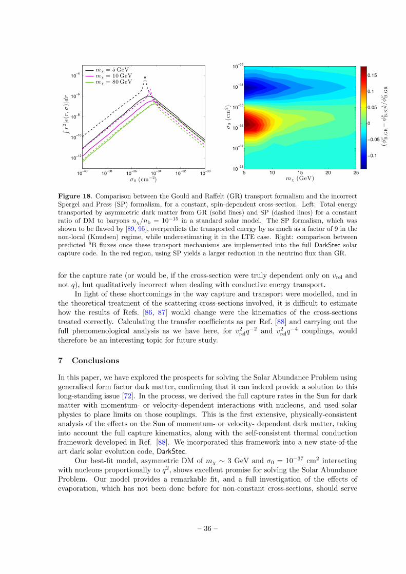
10−40

10−38

10−36

10−34

10−32

10−30

10−12

10−10

10−8

10−6

10−4

σ0 (cm−2)

∫r2|ǫ(r,σ)|dr

mχ = 5GeVmχ = 10 GeVmχ = 80 GeV

mχ (GeV)

σ0(cm

2)

5 10 15 20 2510

−38

10−37

10−36

10−35

10−34

10−33

(φν B,G

R−

φν B,SP)/φν B,G

R

−0.1

−0.05

0

0.05

0.1

0.15

Figure 18. Comparison between the Gould and Raffelt (GR) transport formalism and the incorrectSpergel and Press (SP) formalism, for a constant, spin-dependent cross-section. Left: Total energytransported by asymmetric dark matter from GR (solid lines) and SP (dashed lines) for a constantratio of DM to baryons nχ/nb = 10−15 in a standard solar model. The SP formalism, which wasshown to be flawed by [89, 95], overpredicts the transported energy by as much as a factor of 9 in thenon-local (Knudsen) regime, while underestimating it in the LTE case. Right: comparison betweenpredicted 8B fluxes once these transport mechanisms are implemented into the full DarkStec solarcapture code. In the red region, using SP yields a larger reduction in the neutrino flux than GR.

for the capture rate (or would be, if the cross-section were truly dependent only on vrel andnot q), but qualitatively incorrect when dealing with conductive energy transport.

In light of these shortcomings in the way capture and transport were modelled, and inthe theoretical treatment of the scattering cross-sections involved, it is difficult to estimatehow the results of Refs. [86, 87] would change were the kinematics of the cross-sectionstreated correctly. Calculating the transfer coefficients as per Ref. [88] and carrying out thefull phenomenological analysis as we have here, for v2relq

−2 and v2relq−4 couplings, would

therefore be an interesting topic for future study.

7 Conclusions

In this paper, we have explored the prospects for solving the Solar Abundance Problem usinggeneralised form factor dark matter, confirming that it can indeed provide a solution to thislong-standing issue [72]. In the process, we derived the full capture rates in the Sun for darkmatter with momentum- or velocity-dependent interactions with nucleons, and used solarphysics to place limits on those couplings. This is the first extensive, physically-consistentanalysis of the effects on the Sun of momentum- or velocity- dependent dark matter, takinginto account the full capture kinematics, along with the self-consistent thermal conductionframework developed in Ref. [88]. We incorporated this framework into a new state-of-theart dark solar evolution code, DarkStec.

Our best-fit model, asymmetric DM of mχ ∼ 3 GeV and σ0 = 10−37 cm2 interactingwith nucleons proportionally to q2, shows excellent promise for solving the Solar AbundanceProblem. Our model provides a remarkable fit, and a full investigation of the effects ofevaporation, which has not been done before for non-constant cross-sections, should serve

– 36 –

as a cross-check on the consistency of such a scenario. The prospects for detecting such aparticle at the next round of direct detection experiments, and in the next run of the LHC,also appear very promising.

Acknowledgements

We thank Wan-lei Guo for providing us with numerical values of the XENON constraints forgeneralised form factor DM models. This work was done with partial support from NSERC(Canada), FQRNT (Quebec), STFC (UK) and European contracts FP7-PEOPLE-2011-ITN,PITN-GA-2011-289442-INVISIBLES, ESP2013-41268-R (MINECO) and 2014SGR-1458 (Gen-eralitat de Catalunya). Calculations were performed on SOM2 at IFIC (Universitat deValencia – CSIC) funded by PROMETEO/2009/116, PROMETEOII/2014/050 and FPA2011-29678.

References

[1] R. Bernabei, P. Belli, et. al., First results from DAMA/LIBRA and the combined results withDAMA/NaI, European Physical Journal C 56 (2008) 333, [arXiv:0804.2741].

[2] CoGeNT Collaboration: C. E. Aalseth, P. S. Barbeau, et. al., Search for an AnnualModulation in a p-Type Point Contact Germanium Dark Matter Detector, Phys. Rev. Lett.107 (2011) 141301, [arXiv:1106.0650].

[3] CRESST Collaboration: G. Angloher, M. Bauer, et. al., Results from 730 kg days of theCRESST-II Dark Matter search, Eur. Phys. J. C 72 (2012) 1971, [arXiv:1109.0702].

[4] CDMS Collaboration: R. Agnese et. al., Dark Matter Search Results Using the SiliconDetectors of CDMS II, Phys. Rev. Lett. 111 (2013) 251301, [arXiv:1304.4279].

[5] XENON10 Collaboration: J. Angle et. al., A search for light dark matter in XENON10 data,Phys. Rev. Lett. 107 (2011) 051301, [arXiv:1104.3088].

[6] XENON100 Collaboration: E. Aprile, M. Alfonsi, et. al., Dark Matter Results from 225 LiveDays of XENON100 Data, Phys. Rev. Lett. 109 (2012) 181301, [arXiv:1207.5988].

[7] COUPP Collaboration: E. Behnke, J. Behnke, et. al., First dark matter search results from a4-kg CF3I bubble chamber operated in a deep underground site, Phys. Rev. D 86 (2012)052001, [arXiv:1204.3094].

[8] SIMPLE Collaboration: M. Felizardo, T. A. Girard, et. al., Final Analysis and Results of thePhase II SIMPLE Dark Matter Search, Phys. Rev. Lett. 108 (2012) 201302,[arXiv:1106.3014].

[9] LUX Collaboration: D. Akerib et. al., First results from the LUX dark matter experiment atthe Sanford Underground Research Facility, Phys. Rev. Lett. 112 (2013) 091303,[arXiv:1310.8214].

[10] R. Agnese, A. J. Anderson, et. al., Search for Low-Mass Weakly Interacting Massive Particleswith SuperCDMS, Phys. Rev. Lett. 112 (2014) 241302, [arXiv:1402.7137].

[11] P. Scott, M. Fairbairn, and J. Edsjo, Dark stars at the Galactic Centre - the main sequence,MNRAS 394 (2009) 82–104, [0809.1871].

[12] S. Turck-Chieze and I. Lopes, Solar-stellar astrophysics and dark matter, Research inAstronomy and Astrophysics 12 (2012) 1107–1138.

[13] K. M. Zurek, Asymmetric Dark Matter: Theories, signatures, and constraints, Phys. Rep. 537(2014) 91–121, [arXiv:1308.0338].

– 37 –

[14] L. M. Krauss, M. Srednicki, and F. Wilczek, Solar System constraints and signatures fordark-matter candidates, Phys. Rev. D 33 (1986) 2079–2083.

[15] T. K. Gaisser, G. Steigman, and S. Tilav, Limits on cold-dark-matter candidates from deepunderground detectors, Phys. Rev. D 34 (1986) 2206–2222.

[16] K. Griest and D. Seckel, Cosmic asymmetry, neutrinos and the Sun., Nucl. Phys. B 283(1987) 681–705.

[17] R. Gandhi, J. L. Lopez, D. V. Nanopoulos, K.-j. Yuan, and A. Zichichi, Scrutinizingsupergravity models through neutrino telescopes, Phys. Rev. D 49 (1994) 3691–3703,[astro-ph/9309048].

[18] A. Bottino, N. Fornengo, G. Mignola, and L. Moscoso, Signals of neutralino dark matter fromearth and sun, Astropart. Phys. 3 (1995) 65–76, [hep-ph/9408391].

[19] L. Bergstrom, J. Edsjo, and P. Gondolo, Indirect detection of dark matter in km-size neutrinotelescopes, Phys. Rev. D 58 (1998) 103519, [hep-ph/9806293].

[20] V. Barger, F. Halzen, D. Hooper, and C. Kao, Indirect search for neutralino dark matter withhigh energy neutrinos, Phys. Rev. D 65 (2002) 075022, [hep-ph/0105182].

[21] Super-Kamiokande Collaboration: S. Desai, Y. Ashie, et. al., Search for dark matter WIMPsusing upward through-going muons in Super-Kamiokande, Phys. Rev. D 70 (2004) 083523,[hep-ex/0404025].

[22] Super-Kamiokande Collaboration: S. Desai, K. Abe, et. al., Study of TeV neutrinos withupward showering muons in Super-Kamiokande, Astropart. Phys. 29 (2008) 42–54,[arXiv:0711.0053].

[23] IceCube Collaboration: R. Abbasi, Y. Abdou, et. al., Limits on a Muon Flux from NeutralinoAnnihilations in the Sun with the IceCube 22-String Detector, Phys. Rev. Lett. 102 (2009)201302, [arXiv:0902.2460].

[24] IceCube Collaboration: R. Abbasi, Y. Abdou, et. al., Limits on a muon flux fromKaluza-Klein dark matter annihilations in the Sun from the IceCube 22-string detector, Phys.Rev. D 81 (2010) 057101, [arXiv:0910.4480].

[25] IceCube Collaboration: R. Abbasi, Y. Abdou, et. al., Multiyear search for dark matterannihilations in the Sun with the AMANDA-II and IceCube detectors, Phys. Rev. D 85 (2012)042002, [arXiv:1112.1840].

[26] Super-Kamiokande Collaboration: T. Tanaka, K. Abe, et. al., An Indirect Search for WeaklyInteracting Massive Particles in the Sun Using 3109.6 Days of Upward-going Muons inSuper-Kamiokande, ApJ 742 (2011) 78, [arXiv:1108.3384].

[27] P. Scott, C. Savage, J. Edsjo, and the IceCube Collaboration: R. Abbasi et al., Use ofevent-level neutrino telescope data in global fits for theories of new physics, JCAP 11 (2012)57, [arXiv:1207.0810].

[28] H. Silverwood, P. Scott, et. al., Sensitivity of IceCube-DeepCore to neutralino dark matter inthe MSSM-25, JCAP 3 (2013) 27, [arXiv:1210.0844].

[29] IceCube Collaboration: M. G. Aartsen, R. Abbasi, et. al., Search for Dark MatterAnnihilations in the Sun with the 79-String IceCube Detector, Phys. Rev. Lett. 110 (2013)131302, [arXiv:1212.4097].

[30] W.-L. Guo, Z.-L. Liang, and Y.-L. Wu, Direct detection and solar capture of dark matter withmomentum and velocity dependent elastic scattering, Nucl. Phys. B 878 (2014) 295–308,[arXiv:1305.0912].

[31] R. Catena, Dark matter signals at neutrino telescopes in effective theories, 1503.04109.

– 38 –

[32] C. Rott, J. M. Siegal-Gaskins, and J. F. Beacom, New sensitivity to solar WIMP annihilationusing low-energy neutrinos, Phys. Rev. D 88 (2013) 055005, [arXiv:1208.0827].

[33] N. Bernal, J. Martn-Albo, and S. Palomares-Ruiz, A novel way of constraining WIMPsannihilations in the Sun: MeV neutrinos, JCAP 1308 (2013) 011, [arXiv:1208.0834].

[34] P. Salati and J. Silk, A stellar probe of dark matter annihilation in galactic nuclei, ApJ 338(1989) 24–31.

[35] A. Bouquet and P. Salati, Life and death of cosmions in stars, A&A 217 (1989) 270–282.

[36] I. V. Moskalenko and L. L. Wai, Dark Matter Burners, ApJ 659 (2007) L29–L32,[astro-ph/0702654].

[37] G. Bertone and M. Fairbairn, Compact stars as dark matter probes, Phys. Rev. D 77 (2008)043515, [arXiv:0709.1485].

[38] D. Spolyar, K. Freese, and P. Gondolo, Dark Matter and the First Stars: A New Phase ofStellar Evolution, Phys. Rev. Lett. 100 (2008) 051101, [arXiv:0705.0521].

[39] M. Fairbairn, P. Scott, and J. Edsjo, The zero age main sequence of WIMP burners, Phys.Rev. D 77 (2008) 047301, [arXiv:0710.3396].

[40] P. Scott, J. Edsjo, and M. Fairbairn, Low mass stellar evolution with WIMP capture andannihilation, in Dark Matter in Astroparticle and Particle Physics: Dark 2007 (H. K.Klapdor-Kleingrothaus and G. F. Lewis, eds.), World Scientific, Singapore (2008) 387–392,[arXiv:0711.0991].

[41] F. Iocco, Dark Matter Capture and Annihilation on the First Stars: Preliminary Estimates,ApJ 677 (2008) L1–L4, [arXiv:0802.0941].

[42] F. Iocco, A. Bressan, et. al., Dark matter annihilation effects on the first stars, MNRAS 390(2008) 1655–1669, [arXiv:0805.4016].

[43] J. Casanellas and I. Lopes, The Formation and Evolution of Young Low-mass Stars withinHalos with High Concentration of Dark Matter Particles, ApJ 705 (2009) 135–143,[arXiv:0909.1971].

[44] E. Ripamonti, F. Iocco, et. al., First star formation with dark matter annihilation, MNRAS406 (2010) 2605–2615, [arXiv:1003.0676].

[45] E. Zackrisson, P. Scott, et. al., Finding High-redshift Dark Stars with the James Webb SpaceTelescope, ApJ 717 (2010) 257–267, [arXiv:1002.3368].

[46] E. Zackrisson, P. Scott, et. al., Observational constraints on supermassive dark stars, MNRAS407 (2010) L74–L78, [arXiv:1006.0481].

[47] P. Scott, A. Venkatesan, et. al., Impacts of Dark Stars on Reionization and Signatures in theCosmic Microwave Background, ApJ 742 (2011) 129, [arXiv:1107.1714].

[48] D. E. Kaplan, M. A. Luty, and K. M. Zurek, Asymmetric Dark Matter, Phys. Rev. D 79(2009) 115016, [arXiv:0901.4117].

[49] I. P. Lopes, J. Silk, and S. H. Hansen, Helioseismology as a new constraint on supersymmetricdark matter, MNRAS 331 (2002) 361–368, [astro-ph/0111530].

[50] A. Bottino, G. Fiorentini, et. al., Does solar physics provide constraints to weakly interactingmassive particles?, Phys. Rev. D 66 (2002) 053005, [hep-ph/0206211].

[51] D. T. Cumberbatch, J. Guzik, J. Silk, L. S. Watson, and S. M. West, Light WIMPs in theSun: Constraints from Helioseismology, Phys. Rev. D 82 (2010) 103503, [arXiv:1005.5102].

[52] M. Taoso, F. Iocco, G. Meynet, G. Bertone, and P. Eggenberger, Effect of low mass darkmatter particles on the Sun, Phys. Rev. D 82 (2010) 083509, [arXiv:1005.5711].

– 39 –

[53] I. Lopes and J. Silk, Solar Constraints on Asymmetric Dark Matter, ApJ 757 (2012) 130,[arXiv:1209.3631].

[54] J. N. Bahcall, S. Basu, M. Pinsonneault, and A. M. Serenelli, Helioseismological implicationsof recent solar abundance determinations, ApJ 618 (2005) 1049–1056, [astro-ph/0407060].

[55] S. Basu and H. Antia, Constraining solar abundances using helioseismology, ApJ 606 (2004)L85, [astro-ph/0403485].

[56] J. N. Bahcall, A. M. Serenelli, and S. Basu, 10,000 Standard Solar Models: A Monte CarloSimulation, ApJS 165 (2006) 400–431, [astro-ph/0511337].

[57] W. M. Yang and S. L. Bi, Solar Models with Revised Abundances and Opacities, ApJ 658(2007) L67–L70, [arXiv:0805.3644].

[58] S. Basu and H. M. Antia, Helioseismology and solar abundances, Phys. Rep. 457 (2008)217–283, [arXiv:0711.4590].

[59] A. Serenelli, S. Basu, J. W. Ferguson, and M. Asplund, New Solar Composition: The ProblemWith Solar Models Revisited, ApJ 705 (2009) L123–L127, [arXiv:0909.2668].

[60] C. Allende Prieto, D. L. Lambert, and M. Asplund, The Forbidden Abundance of Oxygen inthe Sun, ApJ 556 (2001) L63–L66, [astro-ph/0106360].

[61] C. Allende Prieto, D. L. Lambert, and M. Asplund, A Reappraisal of the Solar PhotosphericC/O Ratio, ApJ 573 (2002) L137–L140, [astro-ph/0206089].

[62] M. Asplund, N. Grevesse, A. J. Sauval, C. Allende Prieto, and D. Kiselman, Line formationin solar granulation. IV. [O I], O I and OH lines and the photospheric O abundance, A&A417 (2004) 751–768, [astro-ph/0312290].

[63] M. Asplund, N. Grevesse, A. J. Sauval, C. Allende Prieto, and R. Blomme, Line formation insolar granulation. VI. [C I], C I, CH and C2 lines and the photospheric C abundance, A&A431 (2005) 693–705, [astro-ph/0410681].

[64] M. Asplund, N. Grevesse, and A. J. Sauval, The Solar Chemical Composition, in CosmicAbundances as Records of Stellar Evolution and Nucleosynthesis (T. G. Barnes III and F. N.Bash, eds.), Astron. Soc. Pac., San Francisco, ASP Conf. Ser. 336 (2005) 25.

[65] P. Scott, M. Asplund, N. Grevesse, and A. J. Sauval, Line formation in solar granulation.VII. CO lines and the solar C and O isotopic abundances, A&A 456 (2006) 675–688,[astro-ph/0605116].

[66] J. Melendez and M. Asplund, Another forbidden solar oxygen abundance: the [O I] 5577 Aline, A&A 490 (2008) 817–821, [arXiv:0808.2796].

[67] P. Scott, M. Asplund, N. Grevesse, and A. J. Sauval, On the Solar Nickel and OxygenAbundances, ApJ 691 (2009) L119–L122, [arXiv:0811.0815].

[68] M. Asplund, N. Grevesse, A. J. Sauval, and P. Scott, The chemical composition of the Sun,ARA&A 47 (2009) 481–522, [arXiv:0909.0948].

[69] P. Scott, N. Grevesse, et. al., The elemental composition of the Sun. I. The intermediate masselements Na to Ca, A&A 573 (2015) A25, [arXiv:1405.0279].

[70] P. Scott, M. Asplund, N. Grevesse, M. Bergemann, and A. J. Sauval, The elementalcomposition of the Sun. II. The iron group elements Sc to Ni, A&A 573 (2015) A26,[arXiv:1405.0287].

[71] N. Grevesse, P. Scott, M. Asplund, and A. J. Sauval, The elemental composition of the Sun.III. The heavy elements Cu to Th, A&A 573 (2015) A27, [arXiv:1405.0288].

[72] A. C. Vincent, P. Scott, and A. Serenelli, Possible Indication of Momentum-DependentAsymmetric Dark Matter in the Sun, Phys. Rev. Lett. 114 (2015) 081302, [arXiv:1411.6626].

– 40 –

[73] M. Pospelov and T. ter Veldhuis, Direct and indirect limits on the electro-magnetic formfactors of WIMPs, Phys. Lett. B 480 (2000) 181–186, [hep-ph/0003010].

[74] K. Sigurdson, M. Doran, A. Kurylov, R. R. Caldwell, and M. Kamionkowski, Dark-matterelectric and magnetic dipole moments, Phys. Rev. D 70 (2004) 083501, [astro-ph/0406355].

[75] S. Chang, A. Pierce, and N. Weiner, Momentum Dependent Dark Matter Scattering, JCAP1001 (2010) 006, [arXiv:0908.3192].

[76] B. Feldstein, A. L. Fitzpatrick, and E. Katz, Form Factor Dark Matter, JCAP 1001 (2010)020, [arXiv:0908.2991].

[77] B. Feldstein, A. L. Fitzpatrick, E. Katz, and B. Tweedie, A simple explanation for DAMAwith moderate channeling, JCAP 3 (2010) 29, [arXiv:0910.0007].

[78] S. Chang, N. Weiner, and I. Yavin, Magnetic Inelastic Dark Matter, Phys. Rev. D 82 (2010)125011, [arXiv:1007.4200].

[79] A. L. Fitzpatrick and K. M. Zurek, Dark moments and the DAMA-CoGeNT puzzle, Phys.Rev. D 82 (2010) 075004, [arXiv:1007.5325].

[80] V. Barger, W.-Y. Keung, and D. Marfatia, Electromagnetic properties of dark matter: Dipolemoments and charge form factor, Physics Letters B 696 (2011) 74–78, [arXiv:1007.4345].

[81] M. T. Frandsen, F. Kahlhoefer, C. McCabe, S. Sarkar, and K. Schmidt-Hoberg, Theunbearable lightness of being: CDMS versus XENON, JCAP 7 (2013) 23, [arXiv:1304.6066].

[82] E. Del Nobile, G. Gelmini, P. Gondolo, and J.-H. Huh, Generalized halo independentcomparison of direct dark matter detection data, JCAP 10 (2013) 48, [arXiv:1306.5273].

[83] E. Del Nobile, G. B. Gelmini, P. Gondolo, and J.-H. Huh, Direct detection of light anapoleand magnetic dipole DM, JCAP 6 (2014) 2, [arXiv:1401.4508].

[84] K. Kadota and J. Silk, Constraints on light magnetic dipole dark matter from the ILC and SN1987A, Phys. Rev. D 89 (2014) 103528, [arXiv:1402.7295].

[85] R. Catena and P. Gondolo, Global fits of the dark matter-nucleon effective interactions, JCAP9 (2014) 45, [arXiv:1405.2637].

[86] I. Lopes, K. Kadota, and J. Silk, Constraint on Light Dipole Dark Matter fromHelioseismology, ApJ 780 (2014) L15, [arXiv:1310.0673].

[87] I. Lopes, P. Panci, and J. Silk, Helioseismology with Long-range Dark Matter-BaryonInteractions, ApJ 795 (2014) 162, [arXiv:1402.0682].

[88] A. C. Vincent and P. Scott, Thermal conduction by dark matter with velocity andmomentum-dependent cross-sections, JCAP 4 (2014) 19, [arXiv:1311.2074].

[89] A. Gould and G. Raffelt, Thermal conduction by massive particles, ApJ 352 (1990) 654–668.

[90] I. F. M. Albuquerque, C. Perez de los Heros, and D. S. Robertson, Constraints on selfinteracting dark matter from IceCube results, JCAP 2 (2014) 47, [arXiv:1312.0797].

[91] A. Gould, Weakly interacting massive particle distribution in and evaporation from the sun,ApJ 321 (1987) 560–570.

[92] P. Scott, J. Edsjo, and M. Fairbairn, The DarkStars code: a publicly available dark stellarevolution package, in Dark 2009 (H. V. Klapdor-Kleingrothaus & I. V. Krivosheina, ed.),World Scientific (2010) 320–327, [arXiv:0904.2395].

[93] A. Gould, Resonant enhancements in weakly interacting massive particle capture by the earth,ApJ 321 (1987) 571–585.

[94] R. Catena and B. Schwabe, Form factors for dark matter capture by the Sun in effectivetheories, 1501.03729.

– 41 –

[95] A. Gould and G. Raffelt, Cosmion energy transfer in stars - The Knudsen limit, ApJ 352(1990) 669–680.

[96] A. Weiss and H. Schlattl, GARSTEC: the Garching Stellar Evolution Code. The directdescendant of the legendary Kippenhahn code, Ap&SS 316 (2008) 99–106.

[97] A. M. Serenelli, W. C. Haxton, and C. Pena-Garay, Solar Models with Accretion. I.Application to the Solar Abundance Problem, ApJ 743 (2011) 24, [arXiv:1104.1639].

[98] E. G. Adelberger, A. Garcıa, et. al., Solar fusion cross sections. II. The pp chain and CNOcycles, Rev. Mod. Phys. 83 (2011) 195–246, [arXiv:1004.2318].

[99] N. R. Badnell, M. A. Bautista, et. al., Updated opacities from the Opacity Project, MNRAS360 (2005) 458–464, [astro-ph/0410744].

[100] J. W. Ferguson, D. R. Alexander, et. al., Low-Temperature Opacities, ApJ 623 (2005)585–596, [astro-ph/0502045].

[101] F. J. Rogers and A. Nayfonov, Updated and Expanded OPAL Equation-of-State Tables:Implications for Helioseismology, ApJ 576 (2002) 1064–1074.

[102] A. A. Thoul, J. N. Bahcall, and A. Loeb, Element diffusion in the solar interior, ApJ 421(1994) 828–842, [astro-ph/9304005].

[103] P. Scott, M. Fairbairn, and J. Edsjo, Impacts of WIMP dark matter upon stellar evolution:main-sequence stars, in Identification of dark matter 2008 (2008) PoS(idm2008)073,[arXiv:0810.5560].

[104] P. Gondolo, J. Edsjo, et. al., DarkSUSY: computing supersymmetric dark matter propertiesnumerically, JCAP 7 (2004) 8, [astro-ph/0406204].

[105] B. Paxton, EZ to Evolve ZAMS Stars: A Program Derived from Eggleton’s Stellar EvolutionCode, PASP 116 (2004) 699–701, [astro-ph/0405130].

[106] P. P. Eggleton, The evolution of low mass stars, MNRAS 151 (1971) 351.

[107] P. P. Eggleton, Composition changes during stellar evolution, MNRAS 156 (1972) 361.

[108] O. R. Pols, C. A. Tout, P. P. Eggleton, and Z. Han, Approximate input physics for stellarmodelling, MNRAS 274 (1995) 964–974, [astro-ph/9504025].

[109] K. Abe, Y. Hayato, et. al., Solar neutrino results in Super-Kamiokande-III, Phys. Rev. D 83(2011) 052010, [arXiv:1010.0118].

[110] S. Basu, W. J. Chaplin, Y. Elsworth, R. New, and A. M. Serenelli, Fresh Insights on theStructure of the Solar Core, ApJ 699 (2009) 1403–1417, [arXiv:0905.0651].

[111] A. Serenelli, C. Pena-Garay, and W. C. Haxton, Using the standard solar model to constrainsolar composition and nuclear reaction S factors, Phys. Rev. D 87 (2013) 043001,[arXiv:1211.6740].

[112] S. Degl’Innoccenti, W. A. Dziembowski, G. Fiorentini, and B. Ricci, Helioseismology andstandard solar models, Astropart. Phys. 7 (1997) 77–95, [astro-ph/9612053].

[113] I. W. Roxburgh and S. V. Vorontsov, The ratio of small to large separations of acousticoscillations as a diagnostic of the interior of solar-like stars, A&A 411 (2003) 215–220.

[114] S. Basu, W. J. Chaplin, et. al., Solar abundances and helioseismology: Fine structure spacingsand separation ratios of low-degree p modes, ApJ 655 (2007) 660–671, [astro-ph/0610052].

[115] W. J. Chaplin, A. M. Serenelli, et. al., Solar Heavy-Element Abundance: Constraints fromFrequency Separation Ratios of Low-Degree p-Modes, ApJ 670 (2007) 872–884,[arXiv:0705.3154].

[116] J. Goodman, M. Ibe, et. al., Constraints on dark matter from colliders, Phys. Rev. D 82(2010) 116010, [arXiv:1008.1783].

– 42 –

[117] Y. Bai, P. J. Fox, and R. Harnik, The Tevatron at the frontier of dark matter direct detection,JHEP 12 (2010) 48, [arXiv:1005.3797].

[118] P. J. Fox, R. Harnik, R. Primulando, and C.-T. Yu, Taking a razor to dark matter parameterspace at the LHC, Phys. Rev. D 86 (2012) 015010, [arXiv:1203.1662].

[119] K. Cheung, P.-Y. Tseng, Y.-L. S. Tsai, and T.-C. Yuan, Global constraints on effective darkmatter interactions: relic density, direct detection, indirect detection, and collider, JCAP 5(2012) 1, [arXiv:1201.3402].

[120] J. Kumar and D. Marfatia, Matrix element analyses of dark matter scattering andannihilation, Phys. Rev. D 88 (2013) 014035, [arXiv:1305.1611].

[121] T. Aaltonen, B. Alvarez Gonzalez, et. al., Search for Dark Matter in Events with One Jet andMissing Transverse Energy in pp Collisions at s=1.96TeV, Phys. Rev. Lett. 108 (2012)211804, [arXiv:1203.0742].

[122] M. T. Frandsen and S. Sarkar, Asymmetric dark matter and the Sun, Phys. Rev. Lett. 105(2010) 011301, [arXiv:1003.4505].

[123] D. N. Spergel and W. H. Press, Effect of hypothetical, weakly interacting, massive particles onenergy transport in the solar interior, ApJ 294 (1985) 663–673.

– 43 –