General Topology Pete L. Clark - Welcome to the …math.uga.edu/~pete/pointset.pdf · Introduction...

General Topology

Pete L. Clark

Thanks to Kaj Hansen, Scott Higinbotham, Ishfaaq Imtiyas, William Krinsmanand Maddie Locus for pointing out typos in these notes.

Contents

Chapter 1. Introduction to Topology 51. Introduction to Real Induction 52. Real Induction in Calculus 63. Real Induction in Topology 104. The Miracle of Sequences 125. Induction and Completeness in Ordered Sets 136. Dedekind Cuts 17

Chapter 2. Metric Spaces 211. Metric Geometry 212. Metric Topology 243. Convergence 294. Continuity 315. Equivalent Metrics 336. Product Metrics 357. Compactness 408. Completeness 449. Total Boundedness 4810. Separability 5011. Compactness Revisited 5212. Extension Theorems 5713. Completion 6014. Cantor Space 6315. Contractions and Attractions 64

Chapter 3. Introducing Topological Spaces 671. In Which We Meet the Object of Our Affections 672. A Topological Bestiary 703. Alternative Characterizations of Topological Spaces 724. The Set of All Topologies on X 745. Bases, Subbases and Neighborhood Bases 766. The Subspace Topology 787. The Product Topology 818. The Coproduct Topology 869. The Quotient Topology 8810. Initial and Final Topologies 9311. Compactness 9512. Connectedness 10013. Local Compactness and Local Connectedness 10314. The Order Topology 109

3

4 CONTENTS

Chapter 4. Convergence 1131. Introduction: Convergence in Metric Spaces 1132. Sequences in Topological Spaces 1153. Nets 1194. Convergence and (Quasi-)Compactness 1245. Filters 1276. A characterization of quasi-compactness 1337. The correspondence between filters and nets 1348. Notes 137

Chapter 5. Separation and Countability 1411. Axioms of Countability 1412. The Lower Separation Axioms 1453. More on Hausdorff Spaces 1544. Regularity and Normality 1565. P-Ifification 1596. Further Exercises 161

Chapter 6. Embedding, Metrization and Compactification 1631. Completely Regular and Tychonoff Spaces 1632. Urysohn and Tietze 1643. The Tychonoff Embedding Theorem 1664. The Big Urysohn Theorem 1675. A Manifold Embedding Theorem 1686. The Stone-Cech Compactification 170

Chapter 7. Appendix: Very Basic Set Theory 1711. The Basic Trichotomy: Finite, Countable and Uncountable 1712. Order and Arithmetic of Cardinalities 1803. The Calculus of Ordinalities 189

Bibliography 207

CHAPTER 1

Introduction to Topology

1. Introduction to Real Induction

1.1. Real Induction.

Consider for a moment “conventional” mathematical induction. To use it, onethinks in terms of predicates – i.e., statements P (n) indexed by the natural num-bers – but the cleanest enunciation comes from thinking in terms of subsets of N.The same goes for real induction.

Let a x.(RI3) If a < x ≤ b and [a, x) ⊂ S, then x ∈ S.

Theorem 1.1. (Real Induction) For S ⊂ [a, b], the following are equivalent:(i) S is inductive.(ii) S = [a, b].

Proof. (i) =⇒ (ii): let S ⊂ [a, b] be inductive. Seeking a contradiction,suppose S′ = [a, b] \ S is nonempty, so inf S′ exists and is finite.Case 1: inf S′ = a. Then by (RI1), a ∈ S, so by (RI2), there exists y > a such that[a, y] ⊂ S, and thus y is a greater lower bound for S′ then a = inf S′: contradiction.Case 2: a < inf S′ ∈ S. If inf S′ = b, then S = [a, b]. Otherwise, by (RI2) thereexists y > inf S′ such that [inf S′, y] ⊂ S, contradicting the definition of inf S′.Case 3: a < inf S′ ∈ S′. Then [a, inf S′) ⊂ S, so by (RI3) inf S′ ∈ S: contradiction!(ii) =⇒ (i) is immediate. �

Theorem 1.1 is due to D. Hathaway [Ha11] and, independently, to me. But math-ematically equivalent ideas have been around in the literature for a long time:see [Ch19], [Kh23], [Pe26], [Kh49], [Du57], [Fo57], [MR68], [Sh72], [Be82],[Le82], [Sa84], [Do03]. Especially, I acknowledge my indebtedness to a work ofKalantari [Ka07]. I read this paper early in the morning of Tuesday, Septem-ber 7, 2010 and found it fascinating. Kalantari’s formulation works with subsetsS ⊂ [a, b), replaces (RI2) and (RI3) by the single axiom

(RIK) For x ∈ [a, b), if [a, x) ⊂ S, then there exists y > x with [a, y) ⊂ S,1

and the conclusion is that a subset S ⊂ [a, b) satisfying (RI1) and (RIK) must beequal to [a, b). Unfortunately I was a bit confused by Kalantari’s formulation, and

1One also needs the convention [x, x) = {x} here.

5

6 1. INTRODUCTION TO TOPOLOGY

I wrote to Professor Kalantari suggesting the “fix” of replacing (RIK) with (RI2)and (RI3). He wrote back later that morning to set me straight. I was scheduled togive a general interest talk for graduate students in the early afternoon, and I hadplanned to speak about binary quadratic forms. But I found real induction to betoo intriguing to put down, and my talk at 2 pm that day was on real induction (inthe formulation of Theorem 1.1). This was, perhaps, the best received non-researchlecture I have ever given, and I was motivated to develop these ideas in more detail.

In 2011 D. Hathaway published a short note “Using Continuity Induction” [Ha11]giving an all but identical formulation: instead of (RI2), he takes

(RI2H) If a ≤ x < b, then x ∈ S =⇒ [x, x+ δ) ⊂ S for some δ > 0.

(RI2) and (RI2H) are equivalent: [x, x + δ2 ] ⊂ [x, x + δ) ⊂ [x, x + δ]. Hathaway

and I arrived at our formulations completely independently. Moreover, when firstformulating real induction I too used (RI2H), but soon changed it to (RI2) with aneye to a certain more general inductive principle that we will meet later.

2. Real Induction in Calculus

We begin with the “interval theorems” from honors (i.e., theoretical) calculus: thesefundamental results all begin the same way: “Let f : [a, b] → R be a continuousfunction.” Then they assert four different conclusions. One of these conclusionsis truly analytic in character, but the other three are really the source of all topology.

To be sure, let’s begin with the definition of a continuous real-valued functionf : I → R defined on a subinterval of R: let x be a point of I. Then f is continu-ous at x if for all ε > 0, there is δ > 0 such that for all y ∈ I, if |x − y| ≤ δ then|f(x)− f(y)| ≤ ε. f is continuous if it is continuous at every point of I.

Let us also record the following definition: f : I → R is uniformly continu-ous if for all ε > 0, there is δ > 0 such that for all y ∈ I, if |x − y| ≤ δ then|f(x)− f(y)| ≤ ε. Note that this is stronger than continuity in a rather subtle way:the only difference is that in the definition of continuity, the δ is allowed to dependon ε but also on the point x; in uniform continuity, δ is only allowed to depend onε: there must be one δ which works simultaneously for all x ∈ I.

Exercise 2.1. a) Show – from scratch – that each of the following functionsis continuous but not uniformly continuous.(i) f : R→ R, f(x) = x2.(ii) g : (0, 1)→ R, f(x) = 1

x .b) Recall that a subset S ⊂ R is bounded if S ⊂ [−M,M ] for some M ≥ 0. Showthat if I is a bounded interval and f : I → R is uniformly continuous, then f isbounded (i.e., f(I) is bounded). Notice: by part a), continuity is not enough.

Theorem 1.2. (Intermediate Value Theorem (IVT)) Let f : [a, b] → R be acontinuous function, and let L be any number in between f(a) and f(b). Then thereexists c ∈ [a, b] such that f(c) = L.

Proof. It is easy to reduce the theorem to the following special case: letf : [a, b]→ R be continuous and nowhere zero. If f(a) > 0, then f(b) > 0.

2. REAL INDUCTION IN CALCULUS 7

Let S = {x ∈ [a, b] | f(x) > 0}. Then f(b) > 0 iff b ∈ S. We will showS = [a, b].(RI1) By hypothesis, f(a) > 0, so a ∈ S.(RI2) Let x ∈ S, x < b, so f(x) > 0. Since f is continuous at x, there exists δ > 0such that f is positive on [x, x+ δ], and thus [x, x+ δ] ⊂ S.(RI3) Let x ∈ (a, b] be such that [a, x) ⊂ S, i.e., f is positive on [a, x). We claimthat f(x) > 0. Indeed, since f(x) 6= 0, the only other possibility is f(x) < 0, but ifso, then by continuity there would exist δ > 0 such that f is negative on [x− δ, x],i.e., f is both positive and negative at each point of [x− δ, x]: contradiction! �

In the first examples of mathematical induction the statement itself is of the form“For all n ∈ N, P (n) holds”, so it is clear what the induction hypothesis shouldbe. However, mathematical induction is much more flexible and powerful than thisonce one learns to try to find a statement P (n) whose truth for all n will give thedesired result. She who develops skill at “finding the induction hypothesis” acquiresa formidable mathematical weapon: for instance the Arithmetic-Geometric MeanInequality, the Fundamental Theorem of Arithmetic, and the Law of QuadraticReciprocity have all been proved in this way; in the last case, the first proof given(by Gauss) was by induction.

Similarly, to get a Real Induction proof properly underway, we need to find asubset S ⊂ [a, b] for which the conclusion S = [a, b] gives us the result we want, andfor which our given hypotheses are suitable for “pushing from left to right”. If wecan find the right set S then we are, quite often, more than halfway there: the restmay take a little while to write out but is relatively straightforward to produce.

Theorem 1.3. (Extreme Value Theorem (EVT))Let f : [a, b]→ R be continuous. Then:

a) f is bounded.b) f attains a minimum and maximum value.

Proof. a) Let S = {x ∈ [a, b] | f : [a, x]→ R is bounded}.(RI1): Evidently a ∈ S.(RI2): Suppose x ∈ S, so that f is bounded on [a, x]. But then f is continuousat x, so is bounded near x: for instance, there exists δ > 0 such that for ally ∈ [x− δ, x+ δ], |f(y)| ≤ |f(x)|+ 1. So f is bounded on [a, x] and also on [x, x+ δ]and thus on [a, x+ δ].(RI3): Suppose x ∈ (a, b] and [a, x) ⊂ S. Now beware: this does not say that fis bounded on [a, x): rather it says that for all a ≤ y < x, f is bounded on [a, y].These are different statements: for instance, f(x) = 1

x−2 is bounded on [0, y] for all

y < 2 but it is not bounded on [0, 2). But of course this f is not continuous at 2.So we can proceed almost exactly as we did above: since f is continuous at x, thereexists 0 < δ < x− a such that f is bounded on [x− δ, x]. But since a < x− δ < xwe know f is bounded on [a, x− δ], so f is bounded on [a, x].b) Let m = inf f([a, b]) and M = sup f([a, b]). By part a) we have

−∞ < m ≤M <∞.

We want to show that there exist xm, xM ∈ [a, b] such that f(xm) = m, f(xM ) = M ,i.e., that the infimum and supremum are actually attained as values of f . Supposethat there does not exist x ∈ [a, b] with f(x) = m: then f(x) > m for all x ∈ [a, b]

and the function gm : [a, b]→ R by gm(x) = 1f(x)−m is defined and continuous. By

the result of part a), gm is bounded, but this is absurd: by definition of the infimum,f(x)−m takes values less than 1

n for any n ∈ Z+ and thus gm takes values greaterthan n for any n ∈ Z+ and is accordingly unbounded. So indeed there must existxm ∈ [a, b] such that f(xm) = m. Similarly, assuming that f(x) < M for all x ∈[a, b] gives rise to an unbounded continuous function gM : [a, b]→ R, x 7→ 1

M−f(x) ,

contradicting part a). So there exists xM ∈ [a, b] with f(xM ) = M . �

Exercise 2.2. Consider the Hansen Interval Theorem (HIT): let f :[a, b]→ R be a continuous function. Then there are real numbers m ≤M such thatf([a, b]) = [m,M ].a) Show that HIT is equivalent to the conjunction of IVT and EVT: that is, proveHIT using IVT and EVT and then show that HIT implies both of them.b) Can you give a direct proof of HIT?

Let f : I → R. For ε, δ > 0, let us say that f is (ε, δ)-uniformly continuouson I – abbreviated (ε, δ)-UC on I – if for all x1, x2 ∈ I, |x1 − x2| < δ implies|f(x1) − f(x2)| < ε. This is a halfway unpacking of the definition of uniformcontinuity: f : I → R is uniformly continuous iff for all ε > 0, there is δ > 0 suchthat f is (ε, δ)-UC on I.

Lemma 1.4. (Covering Lemma) Let a 0,• f is (ε, δ1)-UC on [a, c] and• f is (ε, δ2)-UC on [b, d].Then f is (ε,min(δ1, δ2, c− b))-UC on [a, b].

Proof. Suppose x1 < x2 ∈ I are such that |x1 − x2| < δ. Then it cannot bethe case that both x1 c − b ≥ δ. Thus we musthave either that b ≤ x1 < x2 or x1 < x2 ≤ c. If b ≤ x1 < x2, then x1, x2 ∈ [b, d]and |x1 − x2| < δ ≤ δ2, so |f(x1) − f(x2)| < ε. Similarly, if x1 < x2 ≤ c, thenx1, x2 ∈ [a, c] and |x1 − x2| < δ ≤ δ1, so |f(x1)− f(x2)| < ε. �

Theorem 1.5. (Uniform Continuity Theorem) Let f : [a, b] → R be continu-ous. Then f is uniformly continuous on [a, b].

Proof. For ε > 0, let S(ε) be the set of x ∈ [a, b] such that there exists δ > 0such that f is (ε, δ)-UC on [a, x]. To show that f is uniformly continuous on [a, b], itsuffices to show that S(ε) = [a, b] for all ε > 0. We will show this by Real Induction.(RI1): Trivially a ∈ S(ε): f is (ε, δ)-UC on [a, a] for all δ > 0!(RI2): Suppose x ∈ S(ε), so there exists δ1 > 0 such that f is (ε, δ1)-UC on[a, x]. Moreover, since f is continuous at x, there exists δ2 > 0 such that for allc ∈ [x, x+δ2], |f(c)−f(x)| < ε

2 . Why ε2? Because then for all c1, c2 ∈ [x−δ2, x+δ2],

|f(c1)− f(c2)| = |f(c1)− f(x) + f(x)− f(c2)| ≤ |f(c1)− f(x)|+ |f(c2)− f(x)| < ε.

In other words, f is (ε, δ2)-UC on [x−δ2, x+δ2]. We apply the Covering Lemma tof with a < x− δ2 < x < x+ δ2 to conclude that f is (ε,min(δ, δ2, x− (x− δ2))) =(ε,min(δ1, δ2))-UC on [a, x+ δ2]. It follows that [x, x+ δ2] ⊂ S(ε).(RI3): Suppose [a, x) ⊂ S(ε). As above, since f is continuous at x, there existsδ1 > 0 such that f is (ε, δ1)-UC on [x−δ1, x]. Since x− δ1

2 < x, by hypothesis there

exists δ2 such that f is (ε, δ2)-UC on [a, x− δ12 ]. We apply the Covering Lemma to f

2. REAL INDUCTION IN CALCULUS 9

with a < x−δ1 < x− δ12 < x to conclude that f is (ε,min(δ1, δ2, x− δ1

2 −(x−δ1))) =

(ε,min( δ12 , δ2))-UC on [a, x]. Thus x ∈ S(ε). �

Theorem 1.6. Let f : [a, b]→ R be a continuous function. Then f is Riemannintegrable.

Proof. We will use Darboux’s Integrability Criterion: we must show that forall ε > 0, there exists a partition P of [a, b] such that U(f,P) − L(f,P) < ε. Itis convenient to prove instead the following equivalent statement: for every ε > 0,there exists a partion P of [a, b] such that U(f,P)− L(f,P) < (b− a)ε.

Fix ε > 0, and let S(ε) be the set of x ∈ [a, b] such that there exists a partitionPx of [a, b] with U(f,Px) − L(f,Px) < ε. We want to show b ∈ S(ε), so it sufficesto show S(ε) = [a, b]. In fact it is necessary and sufficient: observe that if x ∈ S(ε)and a ≤ y ≤ x, then also y ∈ S(ε). We will show S(ε) = [a, b] by Real Induction.(RI1) The only partition of [a, a] is Pa = {a}, and for this partition we haveU(f,Pa) = L(f,Pa) = f(a) · 0 = 0, so U(f,Pa)− L(f,Pa) = 0 < ε.(RI2) Suppose that for x ∈ [a, b) we have [a, x] ⊂ S(ε). We must show that thereis δ > 0 such that [a, x + δ] ⊂ S(ε), and by the above observation it is enoughto find δ > 0 such that x + δ ∈ S(ε): we must find a partition Px+δ of [a, x + δ]such that U(f,Px+δ) − L(f,Px+δ) < (x + δ − a)ε). Since x ∈ S(ε), there is apartition Px of [a, x] with U(f,Px) − L(f,Px) < (x − a)ε. Since f is continuousat x, we can make the difference between the maximum value and the minimumvalue of f as small as we want by taking a sufficiently small interval around x: i.e.,there is δ > 0 such that max(f, [x, x + δ]) − min(f, [x, x + δ]) < ε. Now take thesmallest partition of [x, x+ δ], namely P′ = {x, x+ δ}. Then U(f,P′)− L(f,P′) =(x+δ−x)(max(f, [x, x+δ])−min(f, [x, x+δ])) < δε. Thus if we put Px+δ = Px+P′and use the fact that upper / lower sums add when split into subintervals, we have

U(f,Px+δ)− L(f,Px+δ) = U(f,Px) + U(f,P′)− L(f,Px)− L(f,P′)

= U(f,Px)− L(f,Px) + U(f,P′)− L(f,P′) < (x− a)ε+ δε = (x+ δ − a)ε.

(RI3) Suppose that for x ∈ (a, b] we have [a, x) ⊂ S(ε). We must show that x ∈ S(ε).The argument for this is the same as for (RI2) except we use the interval [x− δ, x]instead of [x, x+ δ]. Indeed: since f is continuous at x, there exists δ > 0 such thatmax(f, [x−δ, x])−min(f, [x−δ, x]) < ε. Since x−δ < x, x−δ ∈ S(ε) and thus thereexists a partition Px−δ of [a, x−δ] such that U(f,Px−δ) = L(f,Px−δ) = (x−δ−a)ε.Let P′ = {x− δ, x} and let Px = Px−δ ∪ P′. Then

U(f,Px)− L(f,Px) = U(f,Px−δ) + U(f,P′)− (L(f,Px−δ) + L(f,P′))

= (U(f,Px−δ)− L(f,Px−δ)) + δ(max(f, [x− δ, x])−min(f, [x− δ, x]))

< (x− δ − a)ε+ δε = (x− a)ε. �

Remark 1.7. The standard proof of Theorem 1.6 is to use Darboux’s Integra-bility Criterion and UCT: this is a short, straightforward argument that we leave tothe interested reader. In fact this application of UCT is probably the one place inwhich the concept of uniform continuity plays a critical role in calculus. (Challenge:does your favorite – or least favorite – freshman calculus book discuss uniform con-tinuity? In many cases the answer is “yes” but the treatment is very well hiddenfrom anyone who is not expressly looking for it.) Uniform continuity is hard to fake– how do you explain it without ε’s and δ’s? – so UCT is probably destined to be theblack sheep of the interval theorems. This makes it an appealing challenge to give a

uniform continuity-free proof of Theorem 1.6. In fact Spivak’s text does so [S, pp.292-293]: he establishes equality of the upper and lower integrals by differentiation.This sort of proof goes back at least to M.J. Norris [No52].

3. Real Induction in Topology

Our task is now to “find the topology” in the classic results of the last section. Incalculus, the standard moral one draws from them is that they are (well, maybe notUCT) properties that are satisfied by our intuitive notion of continuous function,and the fact that they are theorems is a sign of the success of the ε, δ definition ofcontinuity.

I want to argue against that – not for all time, but here at least, because it willbe useful to our purposes to do so. I claim that there is something much deepergoing on in the previous results than just the formal definition of continuity. Tosee this, let us suppose that we replace the closed interval [a, b] with the rationalclosed interval

[a, b]Q = {x ∈ Q | a ≤ x ≤ b}.Nothing stops us from defining continuous and uniformly continuous functionsf : [a, b]Q → Q in exactly the same way as before: namely, using the ε, δ defi-nition. (Soon we will see that this is a case of the ε, δ definition of continuity forfunctions between metric spaces.)

Here’s the punchline: by switching from the real numbers to the rationals, none ofthe interval theorems are true. We will except Theorem 1.6 because it is not quiteclear what the definition of integrability of a rational function should be, and it isnot our business to try to mess with this here. But as for the others:

Example 3.1. Let

X = {x ∈ [0, 2]Q | 0 ≤ x2 < 2}, Y = {x ∈ [0, 2]Q | 2 < x2 ≤ 4}.Define f : [0, 2]Q → Q by f(x) = −1 if x ∈ X and f(x) = 1 if x ∈ Y . The firstthing to notice is that f is indeed well-defined on [0, 2]Q: initially one worries aboutthe case x2 = 2, but – I hope you’ve heard! – there are in fact no such rationalnumbers, so no worries. In fact f is continuous: in fact, suppose x2 < 2. Then forany ε > 0 we can choose any δ > 0 such that (x+ δ)2 < 2. But clearly f does notsatisfy the Intermediate Value Property: it takes exactly two values!

Notice that our choice of δ has the strange property that it is independent ofε! This means that the function f is locally constant: there is a small intervalaround any point at which the function is constant. However the δ cannot be takenindependently of ε so f is not uniformly continuous. More precisely, for everyδ > 0 there are rational numbers x, y with x2 < 2 < y2 and |x − y| < δ, and then|f(x)− f(y)| = 2.

Exercise 3.1. Construct a locally constant (hence continuous!) function f :[0, 2]Q → Q which is unbounded. Deduce the EVT does not hold for continuousfunctions on [a, b]Q. Deduce that such a function cannot be uniformly continous.

The point of these examples is that there must be some good property of [a, b] itselfthat [a, b]Q lacks. Looking back at the proof of Real Induction we quickly find it:it is the celebrated least upper bound axiom. The least upper bound axiom is

3. REAL INDUCTION IN TOPOLOGY 11

in fact the source of all the goodness of R and [a, b], but because in analysis onedoesn’t study structures which don’t have this property, this can be a bit hardto appreciate. Moreover, there are actually several pleasant topological propertiesthat are all implied by the least upper bound axiom, but become distinct in a moregeneral topological context.

To go further, we now introduce some rudimentary topological concepts for in-tervals in the real line and show how real induction works nicely with these concepts.

A subset U ⊂ R is open if for all x ∈ U , there is ε > 0 such that (x− ε, x+ ε) ⊂ U .That is, a subset is open if whenever it contains a point it contains all pointssufficient close to it. In particular the empty set ∅ and R itself are open.

Exercise 3.2. An interval is open in R iff it is of the form (a, b), (−∞, b) or(a,∞).

We also want to define open subsets of intervals, especially of the closed boundedinterval [a, b]. In this course we will define open sets in several different contextsbefore arriving at the final (for us!) level of generality of topological spaces, butone easy common property is that when we are trying to define open subsets of aset X, we always want to include X as an open subset of itself. Notice that if wedirectly extend the above definition of open sets to [a, b] then this doesn’t work:a ∈ [a, b] but there is no ε > 0 such that (a− ε, a+ ε) ⊂ [a, b].

For now we fix this in the kludgiest way: let I ⊂ R be an interval.2 A subsetU ⊂ I is open if:• For every point x ∈ U which is not an endpoint of I, we have (x− ε, x+ ε) ⊂ Ufor some ε > 0;• If x ∈ U is the left endpoint of I, then there is some ε > 0 such that [x, x+ε) ⊂ I.• If x ∈ U is the right endpoint of I, then there is some ε > 0 such that (x−ε, x] ⊂ I.

Exercise 3.3. Show: a subset U of an interval I is open iff whenever U con-tains a point, it contains all points of I which lie sufficiently close to it.

Let A be a subset of an interval I. A point x ∈ I is a limit point of A in I if forall ε > 0, (x− ε, x+ ε) contains a point of A other than x.

Exercise 3.4. Let I be an interval in I. Show that except in the case in whichI consists of a single point, every point of I is a limit point of I.

Theorem 1.8. (Bolzano-Weierstrass) Every infinite subset of [a, b] has a limitpoint in [a, b].

Proof. Let A be an infinite subset of [a, b], and let S be the set of x in[a, b] such that if A ∩ [a, x] is infinite, it has a limit point. It suffices to show thatS = [a, b], which we prove by Real Induction. As usual, (i) is trivial. Since A∩[a, x)is finite iff A∩ [a, x] is finite, (iii) follows. As for (ii), suppose x ∈ S. If A∩ [a, x] isinfinite, then by hypothesis it has a limit point and hence so does [a, b]. So we mayassume that A∩ [a, x] is finite. Now either there exists δ > 0 such that A∩ [a, x+δ]is finite – okay – or every interval [x, x+ δ] contains infinitely many points of A inwhich case x itself is a limit point of A. �

2Until further notice, “interval” will always mean interval in R.

A subset A ⊂ R is compact if given any family {Ui}i∈I of open subsets of R, ifA ⊂

⋃i∈I Ui, then there is a finite subset J ⊂ I with A ⊂

⋃i∈J Ui. We define

compact subsets of an interval (in R) similarly.

Lemma 1.9. Let A ⊂ R be compact. Then A is bounded and every limit pointof A is an element of A.

Proof. For n ∈ Z+, let Un = (−n, n). Then⋃∞n=1 Un = R, and every finite

union of the Un’s is bounded, so if A is unbounded then A ⊂⋃∞n=1 Un and is not

contained in⋃n∈J An for any finite J ⊂ Z+. Suppose that a is a limit point of A

which does not lie in A. Let Un = (−∞, a− 1n )∪(a+ 1

n ,∞). Then⋃∞n=1 Un = R\A,

so A ⊂⋃n∈Z+ Un, but since a is a limit point of A, there is no finite subset J ⊂ Z+

with A ⊂⋃n∈J Un. �

Theorem 1.10. (Heine-Borel) The interval [a, b] is compact.

Proof. For an open covering U = {Ui}i∈I of [a, b], let

S = {x ∈ [a, b] | U ∩ [a, x] has a finite subcovering}.We prove S = [a, b] by Real Induction. (RI1) is clear. (RI2): If U1, . . . , Un covers[a, x], then some Ui contains [x, x+δ] for some δ > 0. (RI3): if [a, x) ⊂ S, let ix ∈ Ibe such that x ∈ Uix , and let δ > 0 be such that [x− δ, x] ∈ Uix . Since x− δ ∈ S,there is a finite J ⊂ I with

⋃i∈J Ui ⊃ [a, x− δ], so {Ui}i∈J ∪ Uix covers [a, x]. �

Proposition 1.11. a) IVT implies the connectedness of [a, b]: if A,B are opensubsets of [a, b] such that A ∩ B = ∅ and A ∪ B = [a, b], then either A = ∅ orB = ∅.b) The connectedness of [a, b] implies IVT.

Proof. In both cases we will argue by contraposition.a) Suppose [a, b] = A ∪ B, where A and B are nonempty open subsets such thatA ∩B = ∅. Then function f : [a, b]→ R which sends x ∈ A 7→ 0 and x ∈ B 7→ 1 iscontinuous but does not have the Intermediate Value Property.b) If IVT fails, there is a continuous function f : [a, b] → R and A < B < C suchthat A,C ∈ f([a, b]) but B /∈ f([a, b]). Let

U = {x ∈ [a, b] | f(x) < B}, V = {x ∈ [a, b] | B < f(x)}.Then U and V are open sets – the basic principle here is that if a continuous functionsatisfies a strict inequality at a point, then it satisfies the same strict inequality insome small interval around the point – which partition [a, b]. �

4. The Miracle of Sequences

Lemma 1.12. (Rising Sun [NP88]) Every infinite sequence in the real line3 hasa monotone subsequence.

Proof. Let us say that m ∈ Z+ is a peak of the sequence {an} if for all n > mwe have an < am. Suppose first that there are infinitely many peaks. Then anysequence of peaks forms a strictly decreasing subsequence, hence we have founda monotone subsequence. So suppose on the contrary that there are only finitelymany peaks, and let N ∈ N be such that there are no peaks n ≥ N . Since n1 = Nis not a peak, there exists n2 > n1 with an2

≥ an1. Similarly, since n2 is not a peak,

3Or any ordered set: see §5.

5. INDUCTION AND COMPLETENESS IN ORDERED SETS 13

there exists n3 > n2 with an3≥ an2

. Continuing in this way we construct an infinite(not necessarily strictly) increasing subsequence an1 , an2 , . . . , ank , . . .. Done! �

Theorem 1.13. (Sequential Bolzano-Weierstrass) Every sequence in [a, b] ad-mits a convergent subsequence.

Proof. Let {xn} be a sequence in [a, b]. By the Rising Sun Lemma, {xn}admits a monotone subsequence. A bounded increasing (resp. decreasing) sequenceconverges to its supremum (resp. infimum). �

Exercise 4.1. (Bolzano-Weierstrass = Sequential Bolzano-Weierstrass)a) Suppose that every infinite subset of [a, b] has a limit point in [a, b]. Show thatevery sequence in [a, b] admits a convergent subsequence.b) Suppose that every sequence in [a, b] admits a convergent subsequence. Show thatevery infinite subset of [a, b] has a limit point in [a, b].

Theorem 1.14. Sequential Bolzano-Weierstrass implies EVTa).

Proof. Seeking a contradiction, let f : [a, b]→ R be an unbounded continuousfunction. Then for each n ∈ Z+ we may choose xn ∈ [a, b] such that |f(xn)| ≥ n.By Theorem 4.1, after passing to a subsequence (which, as usual, we will suppressfrom our notation) we may suppose that xn converges, say to α ∈ [a, b]. Since f iscontinuous, f(xn)→ f(α), so in particular {f(xn)} is bounded...contradiction!(With regard to the attainment of extrema, we have no improvement to offer onthe simple argument using suprema / infima given in the proof of Theorem 1.3. �

Theorem 1.15. Sequential Bolzano-Weierstrass implies UCT (Theorem 1.5).

Proof. Seeking a contradiction, let f : [a, b] → R be continuous but notuniformly continuous. Then there is ε > 0 such that for all n ∈ Z+, there arexn, yn ∈ [a, b] with |xn − yn| < 1

n and |f(xn)− f(yn)| ≥ ε. By Theorem 1.13, afterpassing to a subsequence (notationally suppressed!) xn converges to some α ∈ [a, b],and thus also yn → α. Since f is continuous f(xn) and f(yn) both converge tof(α), hence for sufficiently large n, |f(xn)− f(yn)| < ε: contradiction! �

5. Induction and Completeness in Ordered Sets

5.1. Introduction to Ordered Sets.

Consider the following properties of a binary relation ≤ on a set X:(Reflexivity) For all x ∈ X, x ≤ x.(Anti-Symmetry) For all x, y ∈ X, if x ≤ y and y ≤ x, then x = y.(Transitivity) For all x, y, z ∈ X, if x ≤ y and y ≤ z, then x ≤ z.(Totality) For all x, y ∈ X, either x ≤ y or y ≤ x.A relation which satisfies reflexivity and transitivity is called a quasi-ordering. Arelation which satisfies reflexivity, anti-symmetry and transitivity is called a par-tial ordering. A relation which satisfies all four properties is called an ordering(sometimes a total or linear ordering). An ordered set is a pair (X,≤) whereX is a set and ≤ is an ordering on X.

Rather unsurprisingly, we write x < y when x ≤ y and x 6= y. We also writex ≥ y when y ≤ x and x > y when x ≥ y and x 6= y.

Ordered sets are a basic kind of mathematical structure which induces a topo-logical structure. (It is not yet supposed to be clear exactly what this means.)Moreover they allow an inductive principle which generalizes Real Induction.

A bottom element of an ordered set is an element which is strictly less thanevery other element of the set. Clearly bottom elements are unique if they exist,and clearly they may or may not exist: the natural numbers N have 0 as a bottomelement, and the integers do not have a bottom element. We will denote the bottomelement of an ordered set, when it exists, by B.

If an ordered set does not have a bottom element, we can add one. Let X bean ordered set without a bottom element, choose any B /∈ X, let XB = X ∪ {B},and extend the ordering to B by taking B < x for all x ∈ X.4

There is an entirely parallel discussion for top elements T.

Example 5.1. Starting from the empty set – which is an ordered set! – andapplying the bottom element construction n times, we get a linearly ordered set withn elements. Similarly for applying the top element construction n times.

We will generally suppress the ≤ when speaking about ordered sets and simplyrefer to “the ordered set X”.

Let X and Y be ordered sets. A function f : X → Y is:• increasing (or isotone) if for all x1 ≤ x2 ∈ X, f(x1) ≤ f(x2) in Y ;• strictly increasing if for all x1 < x2 in X, f(x1) < f(x2);• decreasing (or antitone) if for all x1 ≤ x2 in X, f(x1) ≥ f(x2);• strictly decreasing if for all x1 < x2 in X, f(x1) > f(x2).

This directly generalizes the use of these terms in calculus. But now we takethe concept more seriously: we think of orderings on X and Y as giving structureand we think of isotone maps as being the maps which preserve that structure.

Exercise 5.1. Let f : X → Y be an increasing function between ordered sets.Show that f is strictly increasing iff it is injective.

Exercise 5.2. Let X, Y and Z be ordered sets.a) Show that the identity map 1X : X → X is isotone.b) Suppose that f : X → Y and g : Y → Z are isotone maps. Show that thecomposition g ◦ f : X → Z is an isotone map.c) Suppose that f : X → Y and g : Y → Z are antitone maps. Show that thecomposition g : X → Z is an isotone (not antitone!) map.

Let X and Y be ordered sets. An order isomorphism is an isotone map f : X →Y for which there exists an isotone inverse function g : Y → X.

Exercise 5.3. Let X and Y be ordered sets, and let f : X → Y be an isotonebijection. Show that f is an order isomorphism.

4This procedure works even if X already has a bottom element, except with the minor snagthat our suggested notation now has us denoting two different elements by B. We dismiss this as

being beneath our pay grade.

5. INDUCTION AND COMPLETENESS IN ORDERED SETS 15

Exercise 5.4. a) Which linear functions f : R→ R are order isomorphisms?b) Let d ∈ Z+. Show that there is a degree d polynomial order isomorphismP : R→ R iff d is odd.

Exercise 5.5. a) Let f : R → R be a continuous bijection. Show: f is eitherincreasing or decreasing.b) Let f : R → R be a bijection which is either increasing or decreasing. Show: fis continuous.

We say that a property of an ordered set is order-theoretic if whenever an orderedset possesses that property, every order-isomorphic set has that property.

Example 5.2. The following are all order-theoretic properties: being nonempty,being finite, being infinite, having a given cardinality (indeed these are all propertiespreserved by bijections of sets), having a bottom element, having a top element, beingdense.

Let a < b be elements in an ordered set X. We define

[a, b] = {x ∈ X | a ≤ x ≤ b},

(a, b] = {x ∈ X | a < x ≤ b},

[a, b) = {x ∈ X | a ≤ x < b},

(a, b) = {x ∈ X | a < x < b,

(−∞, b] = {x ∈ S | x ≤ b},

(−∞, b) = {x ∈ S | x < b},

[a,∞) = {x ∈ S | a ≤ x},

(a,∞) = {x ∈ S | a < x}.An interval in X is any of the above sets together with ∅ and X itself. We callintervals of the form ∅, (a, b), (−∞, b), (a,∞) and X open intervals. We callintervals of the form [a, b], (−∞, b] and [a,∞) closed intervals.

Exercise 5.6. a) Let a < b and c < d be real numbers. Show that [a, b] and[c, d] are order-isomorphic.b) Let a < b. Show that (a, b) is order-isomorphic to R.c) Classify all intervals in R up to order-isomorphism.

Let x < y be elements in an ordered set. We say that y covers x if (x, y) = ∅: inother words, y is the bottom element of the subset of all elements which are greaterthan x. We say y is the successor of x and write y = x+. Similarly, we say thatx is the predecessor of y and write x = y−. Clearly an element in an ordered setmay or may not have a successor or a predecessor: in Z, every element has both;in R, no element has either one. An element x of an ordered set is left-discrete ifx = B or x has a predecessor and right discrete x = T or x has a successor. Anordered set is discrete if every element is left-discrete and right-discrete.

At the other extreme, an ordered set X is dense if for all a < b ∈ X, thereexists c with a < c < b.

Exercise 5.7. Let X be an ordered set with at least two elements. Show thatthe following are equivalent:(i) No element x 6= B of X is left-discrete.(ii) No element x 6= T of X is right-discrete.(iii) X is dense.

Exercise 5.8. For a linearly ordered set X, we define the order dual X∨ tobe the ordered set with the same underlying set as X but with the ordering reversed:that is, for x, y ∈ X∨, we have x ≤ y ⇐⇒ y ≤ x in X.a) Show that X has a top element (resp. a bottom element) ⇐⇒ X∨ has a bottomelement (resp. a top element).b) Show that X is well-ordered iff X∨ satisfies the ascending chain condition.c) Suppose X is finite. Show that X ∼= X∨ (order-isomorphic).d) Determine which intervals I in R are isomorphic to their order-duals.

Let (X1,≤1) and (X2,≤2) be ordered spaces. We define the lexicographic order≤ on the Cartesian product X1 ×X2 as follows: (x1, x2) ≤ (y1, y2) iff x1 < y1 or(x1 = y1 and x2 ≤ y2).

Exercise 5.9.a) Show: the lexicographic ordering is indeed an ordering on X1 ×X2.b) Show: if X1 and X2 are both well-ordered, so is X1 ×X2.c) Extend the lexicographic ordering to finite products X1 ×Xn.(N.B.: It can be extended to infinite products as well...)

5.2. Completeness and Dedekind Completeness.

The characteristic property of the real numbers among ordered fields is the leastupper bound axiom: every nonempty subset which is bounded above has a leastupper bound. But this axiom says nothing about the algebraic operations + and·: it is purely order-theoretic. In fact, by pursuing its analogue in an arbitraryordered set we will get an interesting and useful generalization of Real Induction.

For a subset S of a linearly ordered set X, a supremum supS of S is a leastelement which is greater than or equal to every element of S, and an infimuminf S of S is a greatest element which is less than or equal to every element of S.X is complete if every subset has a supremum; equivalently, if every subset hasan infimum. If X is complete, it has a least element B = sup∅ and a greatestelement T = inf ∅. X is Dedekind complete if every nonempty bounded abovesubset has a supremum; equivalently, if every nonempty bounded below subset hasan infimum. X is complete iff it is Dedekind complete and has B and T.

Exercise 5.10. Show that an ordered set X is Dedekind complete iff the setobtained by adjoining top and bottom elements to X is complete.

Exercise 5.11. Let X be an ordered set with order-dual X∨.a) Show that X is complete iff X∨ is complete.b) Show that X is Dedekind complete iff X∨ is Dedekind complete.

Exercise 5.12. In the following problem, X and Y are nonempty ordered sets,and Cartesian products are given the lexicographic ordering.a) Show: if X and Y are complete, then X × Y is complete.

6. DEDEKIND CUTS 17

b) Show: R× R in the lexicographic ordering is not Dedekind complete.c) Show: if X × Y is complete, then X and Y are complete.d) Suppose X × Y is Dedekind complete. What can be said about X and Y ?

5.3. Principle of Ordered Induction.

We give an inductive characterization of Dedekind completeness in linearly orderedsets, and apply it to prove three topological characterizations of completeness whichgeneralize familiar results from elementary analysis.

Let X be an ordered set. A set S ⊂ X is inductive if it satisfies:(IS1) There exists a ∈ X such that (−∞, a] ⊂ S.(IS2) For all x ∈ S, either x = T or there exists y > x such that [x, y] ⊂ S.(IS3) For all x ∈ X, if (−∞, x) ⊂ S, then x ∈ S.

Exercise 5.13. Let X be an ordered set with a bottom element B. Show that(IS3) =⇒ (IS1).

Theorem 1.16. (Principle of Ordered Induction) For a linearly ordered set X,the following are equivalent:(i) X is Dedekind complete.(ii) The only inductive subset of X is X itself.

Proof. (i) =⇒ (ii): Let S ⊂ X be inductive. Seeking a contradiction, wesuppose S′ = X \ S is nonempty. Fix a ∈ X satisfying (IS1). Then a is a lowerbound for S′, so by hypothesis S′ has an infimum, say y. Any element less than yis strictly less than every element of S′, so (−∞, y) ⊂ S. By (IS3), y ∈ S. If y = 1,then S′ = {1} or S′ = ∅: both are contradictions. So y < 1, and then by (IS2)there exists z > y such that [y, z] ⊂ S and thus (−∞, z] ⊂ S. Thus z is a lowerbound for S′ which is strictly larger than y, contradiction.(ii) =⇒ (i): Let T ⊂ X be nonempty and bounded below by a. Let S be the setof lower bounds for T . Then (−∞, a] ⊂ S, so S satisfies (IS1).Case 1: Suppose S does not satisfy (IS2): there is x ∈ S with no y ∈ X such that[x, y] ⊂ S. Since S is downward closed, x is the top element of S and x = inf(T ).Case 2: Suppose S does not satisfy (IS3): there is x ∈ X such that (−∞, x) ∈ Sbut x 6∈ S, i.e., there exists t ∈ T such that t < x. Then also t ∈ S, so t is the leastelement of T : in particular t = inf T .Case 3: If S satisfies (IS2) and (IS3), then S = X, so T = {1} and inf T = 1. �

Exercise 5.14. Use the fact that an ordered set X is Dedekind complete iff itsorder dual is to state a downward version of Theorem 1.16.

Exercise 5.15. a) Show that when X is well-ordered, Theorem 1.16 becomesthe principle of transfinite induction.b) Show that when X = [a, b], we recover Real Induction.

6. Dedekind Cuts

Let S be a nonempty ordered set.

A quasi-cut in S is an ordered pair (S1, S2) of subsets S1, S2 ⊂ S with S1 ≤ S2

and S = S1 ∪ S2. It follows immediately that S1 is initial, S2 is final and S1 and


S2 intersect at at most one point.

A cut Λ = (ΛL,ΛR) is a quasi-cut with ΛL ∩ ΛR = ∅; Λ is a Dedekind cutif ΛL and ΛR are both nonempty. We call ΛL and ΛR the initial part and finalpart of the cut, respectively. Any initial (resp. final) subset T ⊂ S is the initialpart of a unique cut: the final (resp. initial) part is S \ T .

For any subset M ⊂ S, we define the downward closure

D(M) = {x ∈ S | x ≤ m for some m ∈M}and the upward closure

U(M) = {x ∈ S | m ≤ x for some m ∈M}.

Exercise 6.1. Let M ⊂ S.a) Show that D(M) is the intersection of all initial subsets of S containing M andthus the unique minimal initial subset containing M .b) Show that U(M) is the intersection of all final subsets of S containing M andthus the unique minimal final subset containing M .

Thus any subset of M determines two (not necessarily distinct) cuts: a cut M+

with initial part D(M) and a cut M− with final part U(M). For α ∈ S, we writeα+ for {α}+ and α− for {α}−.

Exercise 6.2. Let α ∈ S. Show that α+ is the unique cut in which α isthe maximum of the initial part and that α− is the unique cut in which α is theminimum of the final part.

We call cuts of the form α+ and α− principal. Thus a cut fails to be principal iffits initial part has no maximum and its final part has no minimum.

Example 6.1. Let S be a nonempty ordered set.a) The cut (S,∅) is principal iff S has a top element. The cut (∅, S) is principaliff S has a bottom element.b) Let S = R. Then the above two cuts are not principal, but let Λ = (ΛL,ΛR) be aDedekind cut. Then ΛL is bounded above (by any element of ΛR), so let α = sup ΛL.Then either α ∈ ΛL and Λ = α+ or α ∈ ΛR and Λ = α−. Thus every Dedekind cutin R is principal.c) Let S = Q. Then {(−∞,

√2) ∩Q, (

√2,∞)} is a nonprincipal Dedekind cut.

One swiftly draws the following moral.

Theorem 1.17. Let S be an ordered set. Then:a) Every cut in S is principal iff S is complete.b) Every Dedekind cut in S is principal iff S is Dedekind complete.

Exercise 6.3. Prove it.

Now let T be an ordered set, let S ⊂ T be nonempty, and let Λ = (ΛL,ΛR) be acut in S. We say that γ ∈ T realizes Λ in T if ΛL ≤ γ ≤ ΛR. Conversely, to eachγ ∈ T we associate the cut

Λ(γ) = ({x ∈ S | x ≤ γ}, (x ∈ S | x > γ})in S. This is a sinister definition: if γ ∈ S we get Λ(γ) = γ+. (We could haveset things up the other way, but we do need to make a choice one way or the

6. DEDEKIND CUTS 19

other.) The cuts in S which are realized by some element of S are precisely theprincipal cuts, and a principal cut is realized by either one or two elements of S(the latter cannot happen if S is order-dense). Conversely, every element γ ∈ Srealizes precisely two cuts, γ+ and γ−.

Example 6.2. Let S = Q and T = R. The cut {(−∞,√

2) ∩ Q, (√

2,∞)},which is non-principal in S, is realized in T by

√2.

If in an ordered set S we have a nonprincipal cut Λ = (ΛL,ΛR), up to order-isomorphism there is a unique way to add a point γ to S which realizes Λ: namelywe adjoin γ with ΛL < γ < ΛR.

For an ordered set S, we denote by S the set of all cuts in S. We equip S with thefollowing binary relation: for Λ1, Λ2 ∈ S, we put Λ1 ≤ Λ2 if ΛL1 ⊂ ΛL2 .

Proposition 1.18. Let S be an ordered set, and let S be the set of cuts of S.a) The relation ≤ on S is an ordering.b) Each of the maps

ι+ : S → S, x 7→ x+

ι− : S → S, x 7→ x−

is an isotone injection.

Proof. a) The inclusion relation ⊂ is a partial ordering on the power set 2S ;restricting to initial sets we still get a partial ordering. A cut is determined by itsinitial set, so ≤ is certainly a partial ordering on S. The matter of it is to showthat we have a total ordering: equivalently, given any two initial subsets ΛL1 andΛL2 of an ordered set, one is contained in the other. Well, suppose not: if neither iscontained in the other, there is x1 ∈ ΛL1 \ ΛL2 and x2 ∈ ΛL2 \ ΛL1 . We may assumewithout loss of generality that x1 < x2 (otherwise, switch ΛL1 and ΛL2 ): but sinceΛL2 is initial and contains x2, it also contains x1: contradiction.b) This is a matter of unpacking the definitions, and we leave it to the reader. �

Theorem 1.19. Let S be a totally ordered set. The map ι+ : S ↪→ S gives anorder completion of S. That is:a) S is complete: every subset has a supremum and an infimum.b) If X is a complete ordered set and f : S → X is an isotone map, there is an

isotone map f : S → X such that f = f ◦ ι+.

Proof. It will be convenient to identify a cut Λ with its initial set ΛL.a) Let {Λi}i∈I ⊂ S. Put ΛL1 =

⋃i∈I ΛLi and ΛL2 =

⋂i∈I ΛLi . Since unions and

intersections of initial subsets are initial, ΛL1 and ΛL2 are cuts in S, and clearly

ΛL1 = inf{Λi}i∈I , ΛL2 = sup{Λi}i∈I .b) For ΛL ∈ S, we define

f(ΛL) = supx∈ΛL

f(x).

It is easy to see that defining f in this way gives an isotone map with f ◦ι+ = f . �

Theorem 1.20. Let F be an ordered field, and let D(F ) be the Dedekind com-pletion of F . Then D(F ) can be given the structure of a field compatible with itsordering iff the ordering on F is Archimedean.

CHAPTER 2

Metric Spaces

1. Metric Geometry

A metric on a set X is a function d : X ×X → [0,∞) satisfying:

(M1) d(x, y) = 0 ⇐⇒ x = y.(M2) For all x, y ∈ X, d(x, y) = d(y, x).(M3) (Triangle Inequality) For all x, y, z ∈ X, d(x, z) ≤ d(x, y) + d(y, z).

A metric space is a pair (X, d) consisting of a set X and a metric d on X.By the usual abuse of notation, when only one metric on X is under discussion wewill typically refer to “the metric space X.”

Example 1.1. (Discrete Metric) Let X be a set, and for any x, y ∈ X, put

d(x, y) =

{0, x = y

1, x 6= y.

This is a metric on X which we call the discrete metric. We warn the readerthat we will later study a property of metric spaces called discreteness. A setendowed with the discrete metric is a discrete space, but there are discrete metricspaces which are not endowed with the discrete metric.

In general showing that a given function d : X ×X → R is a metric is nontrivial.More precisely verifying the Triangle Inequality is often nontrivial; (M1) and (M2)are usually very easy to check.

Example 1.2. a) Let X = R and take d(x, y) = |x− y|. This is the most basicand important example.b) More generally, let N ≥ 1, let X = RN , and take d(x, y) = ||x − y|| =√∑N

i=1(xi − yi)2. It is very well known but not very obvious that d satisfies the

triangle inequality. This is a special case of Minkowski’s Inequality, which willbe studied later. c) More generally let p ∈ [1,∞), let N ≥ 1, let X = RN and take

dp(x, y) = ||x− y||p =

(N∑i=1

(xi − yi)p) 1p

.

Now the assertion that dp satisfies the triangle inequality is precisely Minkowski’sInequality.

Exercise 1.1. a) Let (X, dx) and (Y, dy) be metric spaces. Show that thefunction

dX×Y : (X × Y )× (X × Y )→ R, ((x1, y1), (x2, y2)) 7→ max(dX(x1, x2), dY (y1, y2))

21

22 2. METRIC SPACES

is a metric on X × Y .b) Extend the result of part a) to finitely many metric spaces (X1, dX1), . . . , (Xn, dXn).c) Let N ≥ 1, let X = RN and take d∞(x, y) = max1≤i≤N |xi − yi|. Show that d∞is a metric.d) For each fixed x, y ∈ RN , show

d∞(x, y) = limp→∞

dp(x, y).

Use this to give a second (more complicated) proof of part c).

Example 1.3. Let (X, d) be a metric space, and let Y ⊂ X be any subset.Show that the restricted function d : Y × Y → R is a metric function on Y .

Example 1.4. Let a ≤ b ∈ R. Let C[a, b] be the set of all continuous functionsf : [a, b]→ R. For f ∈ C[a, b], let

||f || = supx∈[a,b]

|f(x)|.

Then d(f, g) = ||f − g|| is a metric function on C[a, b].Let (X, dx) and (Y, dY ) be metric spaces. A function f : X → Y is an isometricembedding if for all x1, x2 ∈ X, dY (f(x1), f(x2)) = dX(x1, x2). That is, thedistance between any two points in X is the same as the distance between theirimages under f . An isometry is a surjective isometric embedding.

Exercise 1.2. a) Show that every isometric embedding is injective.b) Show that every isometry is bijective and thus admits an inverse function.c) Show that if f : (X, dX)→ (Y, dY ) is an isometry, so is f−1 : (Y, dY )→ (X, dX).

For metric spaces X and Y , let Iso(X,Y ) denote the set of all isometries from Xto Y . Put Iso(X) = Iso(X,X), the isometries from X to itself. According to moregeneral mathematical usage we ought to call elements of Iso(X) “autometries” ofX...but almost no one does.

Exercise 1.3. a) Let f : X → Y and g : Y → Z be isometric embeddings.Show that g ◦ f : X → Z is an isometric embedding.b) Show that IsoX forms a group under composition.c) Let X be a set endowed with the discrete metric. Show that IsoX = SymX isthe group of all bijections f : X → X.d) Can you identify the isometry group of R? Of Eucliedean N -space?

Exercise 1.4. a) Let X be a set with N ≥ 1 elements endowed with the discretemetric. Find an isometric embedding X ↪→ RN−1.b)* Show that there is no isometric embedding X ↪→ RN−2.c) Deduce that an infinite set endowed with the discrete metric is not isometric toany subset of a Euclidean space.

Exercise 1.5. a) Let G be a finite group. Show that there is a finite metricspace X such that IsoX ∼= G (isomorphism of groups).b) Prove or disprove: for every group G, there is a metric space X with IsoX ∼= G?

Let A be a nonempty subset of a metric space X. The diameter of A is

diam(A) = sup{d(x, y) | x, y ∈ A}.Exercise 1.6. a) Show that diamA = 0 iff A consists of a single point.

b) Show that A is bounded iff diamA <∞.c) Show that For any x ∈ X and ε > 0, diamB(x, ε) ≤ 2ε.

1. METRIC GEOMETRY 23

1.1. Further Exercises.

Exercise 1.7. Recall: for sets X,Y we have the symmetric difference

X∆Y = (X \ Y )∐

(Y \X),

the set of elements belonging to exactly one of X and Y (“exclusive or”). Let S bea finite set, and let 2S be the set of all subsets of S. Show that

d : 2S × 2S → N, d(X,Y ) = X∆Y

is a metric function on 2S, called the Hamming metric.

Exercise 1.8. Let X be a metric space.a) Suppose #X ≤ 2. Show that there is an isometric embedding X ↪→ R.b) Let d be a metric function on the set X = {a, b, c}. Show that up to relabellingthe points we may assume

d1 = d(a, b) ≤ d2 = d(b, c) ≤ d3 = d(a, c).

Find necessary and sufficient conditions on d1, d2, d3 such that there is an isometricembedding X ↪→ R. Show that there is always an isometric embedding X ↪→ R2.c) Let X = {•, a, b, c} be a set with four elements. Show that

d(•, a) = d(•, b) = d(•, c) = 1, d(a, b) = d(a, c) = d(b, c) = 2

gives a metric function on X. Show that there is no isometric embedding of X intoany Euclidean space.

Exercise 1.9. Let G = (V,E) be a connected graph. Define a function d :V × V → R by taking d(P,Q) to be the length of the shortest path connecting P toQ.a) Show that d is a metric function on V .b) Show that the metric of Exercise 1.8c) arises in this way.c) Find necessary and/or sufficient conditions for the metric induced by a finiteconnected graph to be isometric to a subspace of some Euclidean space.

Exercise 1.10. Let d1, d2 : X ×X → R be metric functions.a) Show that d1 + d2 : X ×X → R is a metric function.b) Show that max(d1, d2) : X ×X → R is a metric function.

Exercise 1.11. a) Show that for any x, y ∈ R there is f ∈ IsoR such thatf(x) = y.b) Show that for any x ∈ R, there are exactly two isometries f of R such thatf(x) = x.c) Show that every isometric embedding f : R→ R is an isometry.d) Find a metric space X and an isometric embedding f : X → X which is notsurjective.

Exercise 1.12. Consider the following property of a function d : X × X →[0,∞):(M1′) For all x ∈ X, d(x, x) = 0.A pseudometric function is a function d : X × X → [0,∞) satisfying (M1′),(M2) and (M3), and a pseudometric space is a pair (X, d) consisting of a set Xand a pseudometric function d on X.a) Show that every set X admits a pseudometric function.b) Let (X, d) be a pseudometric space. Define a relation ∼ on X by x ∼ y iff

24 2. METRIC SPACES

d(x, y) = 0. Show that ∼ is an equivalence relation.c) Show that the pseudometric function is well-defined on the set X/ ∼ of ∼-equivalence classes: that is, if x ∼ x′ and y ∼ y′ then d(x, y) = d(x′, y′). Show thatd is a metric function on X/ ∼.

1.2. Constructing Metrics.

Lemma 2.1. Let (X, d) be a metric space, and let f : R≥0 → R≥0 be anincreasing, concave function – i.e., −f is convex – with f(0) = 0. Then df = f ◦ dis a metric on X.

Proof. The only nontrivial verification is the triangle inequality. Let x, y, z ∈X. Since d is a metric, we have

d(x, z) ≤ d(x, y) + d(y, z).

Since f is increasing, we have

(1) df (x, z) = f(d(x, z)) ≤ f(d(x, y) + d(y, z)).

Since −f is convex and f(0) = 0, by the Generalized Two Secant Inequality or theInterlaced Secant Inequality, we have for all a ≥ 0 and all t > 0 that

f(a+ t)− f(a)

(a+ t)− a≤ f(t)

t− 0

and thus

(2) f(a+ t) ≤ f(a) + f(t).

Taking a = d(x, y) and t = d(y, z) and combining (1) and (2), we get

df (x, z) ≤ f(d(x, y) + d(y, z)) ≤ df (x, y) + df (y, z). �

Corollary 2.2. Let (X, d) be a metric space, and let α > 0. Let dα : X×X →R be given by

dα(x, y) =αd(x, y)

d(x, y) + 1.

Then dα is a metric on X and diam(X, dα) ≤ α.


Proposition 2.3. Let {(Xi, di)}i∈I be an indexed family of metric spaces. LetX =

∏i∈I Xi. We define d : X → R ∪∞ by

d(x, y) = supi∈I

d(xi, yi).

If d(X ×X) ⊂ R, then d is a metric on X.

2. Metric Topology

Let X be a metric space.

For x ∈ X and ε ≥ 0 we define the open ball

B◦(x, ε) = {y ∈ X | d(x, y) < ε}.and the closed ball

B•(x, ε) = {y ∈ X | d(x, y) ≤ ε}.

2. METRIC TOPOLOGY 25

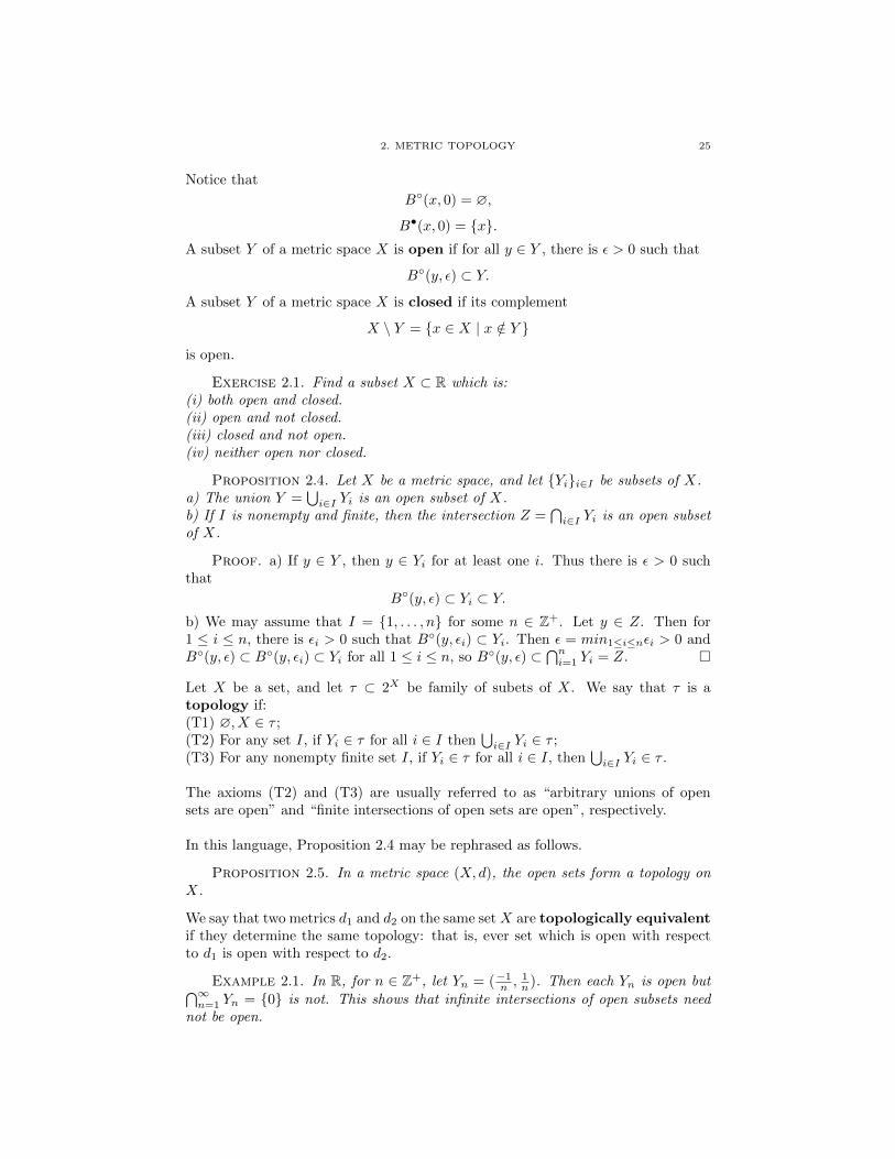
Notice that

B◦(x, 0) = ∅,

B•(x, 0) = {x}.A subset Y of a metric space X is open if for all y ∈ Y , there is ε > 0 such that

B◦(y, ε) ⊂ Y.

A subset Y of a metric space X is closed if its complement

X \ Y = {x ∈ X | x /∈ Y }

is open.

Exercise 2.1. Find a subset X ⊂ R which is:(i) both open and closed.(ii) open and not closed.(iii) closed and not open.(iv) neither open nor closed.

Proposition 2.4. Let X be a metric space, and let {Yi}i∈I be subsets of X.a) The union Y =

⋃i∈I Yi is an open subset of X.

b) If I is nonempty and finite, then the intersection Z =⋂i∈I Yi is an open subset

of X.

Proof. a) If y ∈ Y , then y ∈ Yi for at least one i. Thus there is ε > 0 suchthat

B◦(y, ε) ⊂ Yi ⊂ Y.b) We may assume that I = {1, . . . , n} for some n ∈ Z+. Let y ∈ Z. Then for1 ≤ i ≤ n, there is εi > 0 such that B◦(y, εi) ⊂ Yi. Then ε = min1≤i≤nεi > 0 andB◦(y, ε) ⊂ B◦(y, εi) ⊂ Yi for all 1 ≤ i ≤ n, so B◦(y, ε) ⊂

⋂ni=1 Yi = Z. �

Let X be a set, and let τ ⊂ 2X be family of subets of X. We say that τ is atopology if:(T1) ∅, X ∈ τ ;(T2) For any set I, if Yi ∈ τ for all i ∈ I then

⋃i∈I Yi ∈ τ ;

(T3) For any nonempty finite set I, if Yi ∈ τ for all i ∈ I, then⋃i∈I Yi ∈ τ .

The axioms (T2) and (T3) are usually referred to as “arbitrary unions of opensets are open” and “finite intersections of open sets are open”, respectively.

In this language, Proposition 2.4 may be rephrased as follows.

Proposition 2.5. In a metric space (X, d), the open sets form a topology onX.

We say that two metrics d1 and d2 on the same set X are topologically equivalentif they determine the same topology: that is, ever set which is open with respectto d1 is open with respect to d2.

Example 2.1. In R, for n ∈ Z+, let Yn = (−1n ,

1n ). Then each Yn is open but⋂∞

n=1 Yn = {0} is not. This shows that infinite intersections of open subsets neednot be open.

26 2. METRIC SPACES

Exercise 2.2. a) Show that finite unions of closed sets are closed.b) Show that arbitrary intersections of closed sets are closed.c) Exhibit an infinite union of closed subsets which is not closed.

Exercise 2.3. A metric space X is discrete if every subset Y ⊂ X is open.a) Show that any set endowed with the discrete metric is a discrete metric space.b) A metric space X is uniformly discrete if there is ε > 0 such that for allx 6= y ∈ X, d(x, y) ≥ ε. Show: every uniformly discrete metric space is discrete.c) Let X = { 1

n}∞n=1 as a subspace of R. Show that X is discrete but not uniformly

discrete.

Proposition 2.6. a) Open balls are open sets.b) A subset Y of a metric space X is open iff it is a union of open balls.

Proof. a) Let x ∈ X, let ε > 0, and let y ∈ B◦(x, ε). We claim that B◦(y, ε−d(x, y)) ⊂ B◦(x, ε). Indeed, if z ∈ B◦(y, ε− d(x, y)), then d(y, z) < ε− d(x, y), so

d(x, z) ≤ d(x, y) + d(y, z) < d(x, y) + (ε− d(x, y)) = ε.

b) If Y is open, then for all y ∈ Y , there is εy > 0 such that B◦(ε, y) ⊂ Y . It followsthat Y =

⋃y∈Y B

◦(y, εy). The fact that a union of open balls is open follows from

part a) and the previous result. �

Lemma 2.7. Let Y be a subset of a metric space X. Then the map U 7→ U ∩Yis a surjective map from the open subsets of X to the open subsets of Y .

Exercise 2.4. Prove it. (Hint: for any y ∈ Y and ε > 0, let B◦X(y, ε) ={x ∈ X | d(x, y) < ε} and let B◦Y (y, ε) = {x ∈ Y | d(x, y) < ε}. Then B◦X(y, ε) =B◦Y (y, ε).)

Let X be a metric space, and let Y ⊂ X. We define the interior of Y as

Y ◦ = {y ∈ Y | ∃ε > 0 such that B◦(y, ε) ⊂ Y }.In words, the interior of a set is the collection of points that not only belong to theset, but for which some open ball around the point is entirely contained in the set.

Lemma 2.8. Let Y, Z be subsets of a metric space X.a) All of the following hold:(i) Y ◦ ⊂ Y .(ii) If Y ⊂ Z, then Y ◦ ⊂ Z◦.(iii) (Y ◦)◦ = Y ◦.b) The interior Y ◦ is the largest open subset of Y : that is, Y ◦ is an open subset ofY and if U ⊂ Y is open, then U ⊂ Y ◦.c) Y is open iff Y = Y ◦.


We say that a subset Y is a neighborhood of x ∈ X if x ∈ Y ◦. In particular,a subset is open precisely when it is a neighborhood of each of its points. (Thisterminology introduces nothing essentially new. Nevertheless the situation it en-capsulates it ubiquitous in this subject, so we will find the term quite useful.)

Let X be a metric space, and let Y ⊂ X. A point x ∈ X is an adherent point ofY if every neighborhood N of x intersects Y : i.e., N ∩ Y 6= ∅. Equivalently, forall ε > 0, B(x, ε) ∩ Y 6= ∅.

2. METRIC TOPOLOGY 27

We follow up this definition with another, rather subtly different one, that wewill fully explore later, but it seems helpful to point out the distinction now. ForY ⊂ X, a point x ∈ X is an limit point of Y if every neighborhood of X containsinfinitely many points of Y . Equivalently, for all ε > 0, we have

(B◦(x, ε) \ {x}) ∩ Y 6= ∅.

In particular, every y ∈ Y is an adherent point of Y but not necessarily a limitpoint. For instance, if Y is finite then it has no limit points.

The following is the most basic and important result of the entire section.

Proposition 2.9. For a subset Y of a metric space X, the following are equiv-alent:(i) Y is closed: i.e., X \ Y is open.(ii) Y contains all of its adherent points.(iii) Y contains all of its limit points.

Proof. (i) =⇒ (ii): Suppose that X \ Y is open, and let x ∈ X \ Y . Thenthere is ε > 0 such that B◦(x, ε) ⊂ X \ Y , and thus B◦(x, ε) does not intersect Y ,i.e., x is not an adherent point of Y .(ii) =⇒ (iii): Since every limit point is an adherent point, this is immediate.(iii) =⇒ (i): Suppose Y contains all its limit points, and let x ∈ X \ Y . Thenx is not a limit point of Y , so there is ε > 0 such that (B◦(x, ε) \ {x}) ∩ Y = ∅.Since x /∈ Y this implies B◦(x, ε) ∩ Y = ∅ and thus B◦(x, ε) ⊂ X \ Y . Thus X \ Ycontains an open ball around each of its points, so is open, so Y is closed. �

For a subset Y of a metric space X, we define its closure of Y as

Y = Y ∪ {all adherent points of Y } = Y ∪ {all limit points of Y }.

Lemma 2.10. Let Y,Z be subsets of a metric space X.a) All of the following hold:(KC1) Y ⊂ Y .(KC2) If Y ⊂ Z, then Y ⊂ Z.

(KC3) Y = Y .b) The closure Y is the smallest closed set containing Y : that is, Y is closed,contains Y , and if Y ⊂ Z is closed, then Y ⊂ Z.


Lemma 2.11. Let Y,Z be subsets of a metric space X. Then:a) Y ∪ Z = Y ∪ Z.b) (Y ∩ Z)◦ = Y ◦ ∩ Z◦.

Proof. a) Since Y ∪ Z is a finite union of closed sets, it is closed. ClearlyY ∪ Z ⊃ Y ⊃ Z. So

Y ∪ Z ⊂ Y ∪ Z.Conversely, since Y ⊂ Y ∪ Z we have Y ⊂ Y ∪ Z; similarly Z ⊂ Y ∪ Z. So

Y ∪ Z ⊂ Y ∪ Z.

28 2. METRIC SPACES

b) Y ◦∩Z◦ is a finite intersection of open sets, hence open. Clearly Y ◦∩Z◦ ⊂ Y ∩Z.So

Y ◦ ∩ Z◦ ⊂ (Y ∩ Z)◦.

Conversely, since Y ∩Z ⊂ Y , we have (Y ∩Z)◦ ⊂ Y ◦; similarly (Y ∩Z)◦ ⊂ Z◦. So

(Y ∩ Z)◦ ⊂ Y ◦ ∩ Z◦.�

The similarity between the proofs of parts a) and b) of the preceding result is meantto drive home the point that just as open and closed are “dual notions” – one getsfrom one to the other via taking complements – so are interiors and closures.

Proposition 2.12. Let Y be a subset of a metric space Z. Then

Y ◦ = X \X \ Yand

Y = X \ (X \ Y )◦.

Proof. We will prove the first identity and leave the second to the reader.Our strategy is to show that X \X \ Y is the largest open subset of Y and apply

X.X. Since X \ X \ Y is the complement of a closed set, it is open. Moreover, if

x ∈ X \X \ Y , then x /∈ X \ Y ⊃ X \ Y , so x ∈ Y . Now let U ⊂ Y be open. Then

X \ U is closed and contains X \ Y , so it contains X \ Y . Taking complements

again we get U ⊂ X \X \ Y . �

Proposition 2.13. For a subset Y of a metric space X, consider the following:(i) B1(Y ) = Y \ Y ◦.(ii) B2(Y ) = Y ∩X \ Y .(iii) B3(Y ) = {x ∈ X | every neighborhood N of x intersects both Y and X \ Y }.Then B1(Y ) = B2(Y ) = B3(Y ) is a closed subset of X, called the boundary of Yand denoted ∂Y .


Exercise 2.8. Let Y be a subset of a metric space X.a) Show X = X◦

∐∂X (disjoint union).

b) Show (∂X)◦ = ∅.c) Show that ∂(∂Y ) = ∂Y .

Exercise 2.9. Show: for all closed subsets B of RN , there is a subset Y of RNwith B = ∂Y .

Example 2.2. Let X = R, A = (−∞, 0) and B = [0,∞). Then ∂A = ∂B ={0}, and

∂(A ∪B) = ∂R = ∅ 6= {0} = (∂A) ∪ (∂B);

∂(A ∩B) = ∂∅ = ∅ 6= {0} = (∂A) ∩ (∂B).

Thus the boundary is not as well-behaved as either the closure or interior.

A subset Y of a metric space X is dense if Y = X: explicitly, if for all x ∈ X andall ε > 0, B◦(x, ε) intersects Y .

Example 2.3. Let X be a discrete metric space. The only dense subset of Xis X itself.

3. CONVERGENCE 29

Example 2.4. The subset QN = (x1, . . . , xN ) is dense in RN .

The weight of a metric space is the least cardinality of a dense subspace.

Exercise 2.10.a) Show that the weight of any discrete metric space is its cardinality.b) Show that the weight of any finite metric space is its cardinality.c) Show that every cardinal number arises as the weight of a metric space.

Explicit use of cardinal arithmetic is popular in some circles but not in others. Muchmore commonly used is the following special case: a metric space is separableif it admits a countable dense subspace. Thus the previous example shows thatEuclidean N -space is separable, and a discrete space is separable iff it is countable.


Exercise 2.11. Let Y be a subset of a metric space X. Show:

(Y ◦)◦ = Y ◦

and

Y◦

= Y .

Exercise 2.12. A subset Y of a metric space X is regularly closed if Y = Y ◦

and regularly open if Y = (Y )◦.a) Show that every regularly closed set is closed, every regularly open set is open,and a set is regularly closed iff its complement is regularly open.b) Show that a subset of R is regularly closed iff it is a disjoint union of closedintervals.c) Show that for any subset Y of a metric space X, Y ◦ is regularly closed and Y

◦

is regularly open.

Exercise 2.13. A metric space is a door space if every subset is either openor closed (or both). In a topologically discrete space, every subset is both open andclosed, so such spaces are door spaces, however of a rather uninteresting type. Showthat there is a subset of R which, with the induced metric, is a door space which isnot topologically discrete.

3. Convergence

In any set X, a sequence in X is just a mapping a mapping x : Z+ → X, n 7→ xn.If X is endowed with a metric d, a sequence x in X is said to converge to anelement x of X if for all ε > 0, there exists an N = N(ε) such that for all n ≥ N ,d(x, xn) < ε. We denote this by x→ x or xn → x.

Exercise 3.1. Let x be a sequence in the metric space X, and let L ∈ X. Showthat the following are equivalent.a) The x→ L.b) Every neighbhorhood N of x contains all but finitely many terms of the sequence.More formally, there is N ∈ Z+ such that for all n ≥ N , xn ∈ N .

Proposition 2.14. In any metric space, the limit of a convergent sequence isunique: if L,M ∈ X are such that x→ L and x→M , then L = M .

30 2. METRIC SPACES

Proof. Seeking a contradiction, we suppose L 6= M and put d = d(L,M) > 0.Let B1 = B◦(L, d2 ) and B2 = B◦(M, d2 ), so B1 and B2 are disjoint. Let N1 be suchthat if n ≥ N1, xn ∈ B1, let N2 be such that if n ≥ N2, xn ∈ B2, and letN = max(N1, N2). Then for all n ≥ N , xn ∈ B1 ∩B2 = ∅: contradiction! �

A subsequence of x is obtained by choosing an infinite subset of Z+, writing theelements in increasing order as n1, n2, . . . and then restricting the sequence to thissubset, getting a new sequence y, k 7→ yk = xnk .

Exercise 3.2. Let n : Z+ → Z+ be strictly increasing: for all k1 < k2, nk1 <nk2 . Let x : Z+ → X be a sequence in a set X. Interpret the composite sequencex ◦ n : Z+ → X as a subsequence of x. Show that every subsequence arises inthis way, i.e., by precomposing the given sequence with a unique strictly increasingfunction n : Z+ → Z+.

Exercise 3.3. Let x be a sequence in a metric space.a) Show that if x is convergent, so is every subsequence, and to the same limit.b) Show that conversely, if every subsequence converges, then x converges. (Hint:in fact this is not a very interesting statement. Why?)c) A more interesting converse would be: suppose that there is L ∈ X such that:every subsequence of x which is convergent converges to L. Then x → L. Showthat this fails in R. Show however that it holds in [a, b] ⊂ R.

Let x be a sequence in a metric space X. A point L ∈ X is a partial limit of x ifevery neighborhood N of L contains infinitely many terms of the sequence: moreformally, for all N ∈ Z+, there is n ≥ N such that xn ∈ N .

Lemma 2.15. For a sequence x in a metric space X and L ∈ X, the followingare equivalent:(i) L is a partial limit of x.(ii) There is a subsequence xnk converging to L.

Proof. (i) Suppose L is a partial limit. Choose n1 ∈ Z+ such that d(xn1, L) <

1. Having chosen nk ∈ Z+, choose nk+1 > nk such that d(xnk+1, L) < 1

k+1 . Thenxnk → L.(ii) Let N be any neighborhood of L, so there is ε > 0 such that L ⊂ B◦(L, ε) ⊂ N .If xnk → L, then for every ε > 0 and all sufficiently large k, we have d(xnk , L) < ε,so infinitely many terms of the sequence lie in N . �

The following basic result shows that closures in a metric space can be understoodin terms of convergent sequences.

Proposition 2.16. Let Y be a subset of (X, d). For x ∈ X, the following areequivalent:(i) x ∈ Y .(ii) There exists a sequence x : Z+ → Y such that xn → x.

Proof. (i) =⇒ (ii): Suppose y ∈ Y , and let n ∈ Z+. There is xn ∈ Y suchthat d(y, xn) < ε. Then xn → y.¬ (i) =⇒ ¬ (ii): Suppose y /∈ Y : then there is ε > 0 such that B◦(y, ε) ∩ Y = ∅.Then no sequence in Y can converge to y. �

Corollary 2.17. Let X be a set, and let d1, d2 : X ×X → X be two metrics.

Suppose that for every sequence x ∈ X and every point x ∈ X, we have xd1→ x ⇐⇒

4. CONTINUITY 31

xd2→ x: that is, the sequence x converges to the point x with respect to the metric

d1 it converges to the point x with respect to the metric d2. Then d1 and d2 aretopologically equivalent: they have the same open sets.

Proof. Since the closed sets are precisely the complements of the open sets,it suffices to show that the closed sets with respect to d1 are the same as the closedsets with respect to d2. So let Y ⊂ X and suppose that Y is closed with respect tod1. Then, still with respect to d1, it is equal to its own closure, so by Proposition2.16 for x ∈ X we have that x lies in Y iff there is a sequence y in Y such thaty → x with respect to d1. But now by our assumption this latter characterizationis also valid with respect to d2, so Y is closed with respect to d2. And conversely,of course. �

4. Continuity

Let f : X → Y be metric spaces, and let x ∈ x. We say f is continuous atx if for all ε > 0, there is δ > 0 such that for all x′ ∈ X, if d(x, x′) < δ thend(f(x), f(x′)) < ε. We say f is continuous if it is continuous at every x ∈ X.

Let f : X → Y be a map between metric spaces. A real number C ≥ 0 is aLipschitz constant for f if for all x, y ∈ X, d(f(x), f(y)) ≤ Cd(x, y). A map fis Lipschitz if some C ≥ 0 is a Lipschitz constant for f .

Exercise 4.1. a) Show that a Lipschitz function is continuous.b) Show that if f is Lipschitz, the infimum of all Lipschitz constants for f is aLipschitz constant for f .c) Show that an isometry is Lipschitz.

Lemma 2.18. For a map f : X → Y of metric spaces, the following are equiv-alent:(i) f is continuous.(ii) For every open subset V ⊂ Y , f−1(V ) is open in X.

Proof. (i) =⇒ (ii): Let x ∈ f−1(V ), and choose ε > 0 such thatB◦(f(x), ε) ⊂V . Since f is continuous at x, there is δ > 0 such that for all x′ ∈ B◦(x, δ),f(x′) ∈ B◦(f(x), ε) ⊂ V : that is, B◦(x, δ) ⊂ f−1(V ).(ii) =⇒ (i): Let x ∈ X, let ε > 0, and let V = B◦(f(x), ε). Then f−1(V ) is openand contains x, so there is δ > 0 such that

B◦(x, δ) ⊂ f−1(V ).

That is: for all x′ with d(x, x′) < δ, d(f(x), f(x′)) < ε. �

A map f : X → Y between metric spaces is open if for all open subsets U ⊂ X,f(U) is open in Y . A map f : X → Y is a homeomorphism if it is continuous, isbijective, and the inverse function f−1 : Y → X is continuous. A map f : X → Yis a topological embedding if it is continuous, injective and open.

Exercise 4.2. For a metric space X, let XD be the same underlying set en-dowed with the discrete metric.a) Show that the identity map 1 : XD → X is continuous.b) Show that the identity map 1 : X → XD is continuous iff X is discrete (in thetopological sense: every point of x is an isolated point).

32 2. METRIC SPACES

Example 4.1. a) Let X be a metric space which is not discrete. Then (c.f.Exercise X.X) the identity map 1 : XD → X is bijective and continuous but notopen. The identity map 1 : X → XD is bijective and open but not continuous.b) The map f : R → R by x 7→ |x| is continuous – indeed, Lipschitz with C = 1 –but not open: f(R) = [0,∞).

Exercise 4.3. Let f : R→ R.a) Show that at least one of the following holds:(i) f is increasing: for all x1 ≤ x2, f(x1) ≤ f(x2).(ii) f is decreasing: for all x1 ≤ x2, f(x1) ≥ f(x2).(iii) f is of “Λ-type”: there are a f(c).(iv) f is of “V -type”: there are a f(b) < f(c).b) Suppose f is a continuous injection. Show that f is strictly increasing or strictlydecreasing.c) Let f : R→ R be increasing. Show that for all x ∈ R

supy<x

f(y) ≤ f(x) ≤ infy>x

f(y).

Show that

supy<x

f(y) = f(x) = infy>x

f(y)

iff f is continuous at x.d) Suppose f is bijective and strictly increasing. Show that f−1 is strictly increasing.e) Show that if f is strictly increasing and surjective, it is a homeomorphism.Deduce that every continuous bijection f : R→ R is a homeomorphism.

Lemma 2.19. For a map f : X → Y between metric spaces, the following areequivalent:(i) f is a homeomorphism.(ii) f is continuous, bijective and open.


Proposition 2.20. Let X,Y, Z be metric spaces and f : X → Y , g : Y → Zbe continuous maps. Then g ◦ f : X → Z is continuous.

Proof. Let W be open in Z. Since g is continuous, g−1(W ) is open in Y .Since f is continuous, f−1(g−1(W )) = (g ◦ f)−1(W ) is open in X. �

Proposition 2.21. For a map f : X → Y of metric spaces, the following areequivalent:(i) f is continuous.(ii) If xn → x in X, then f(xn)→ f(x) in Y .

Proof. (i) =⇒ (ii) Let ε > 0. Since f is continuous, by Lemma 2.18 there isδ > 0 such that if x′ ∈ B◦(x, δ), f(x′) ∈ B◦(x, ε). Since xn → x, there is N ∈ Z+

such that for all n ≥ N , xn ∈ B◦(x, δ), and thus for all n ≥ N , f(xn) ∈ B◦(x, ε).¬ (i) =⇒ ¬ (ii): Suppose that f is not continuous: then there is x ∈ X and ε > 0such that for all n ∈ Z+, there is xn ∈ X with d(xn, x) < 1

n and d(f(xn), f(x)) ≥ ε.Then xn → x and f(xn) does not converge to f(x). �

In other words, continuous functions between metric spaces are precisely the func-tions which preserve limits of convergent sequences.

5. EQUIVALENT METRICS 33

Exercise 4.5. a) Let f : X → Y , g : Y → Z be maps of topological spaces. Letx ∈ X. Use ε’s and δ’s to show that if f is continuous at x and g is continuous atf(x) then g ◦ f is continuous at x. Deduce another proof of Proposition 2.20 usingthe (ε, δ)-definition of continuity.b) Give (yet) another proof of Proposition 2.20 using Proposition 2.21.

In higher mathematics, one often meets the phenomenon of rival definitions whichare equivalent in a given context (but may not be in other contexts of interest).Often a key part of learning a new subject is learning which versions of definitionsgive rise to the shortest, most transparent proofs of basic facts. When one definitionmakes a certain proposition harder to prove than another definition, it may be a signthat in some other context these definitions are not equivalent and the propositionis true using one but not the other definition. We will see this kind of phenomenonoften in the transition from metric spaces to topological spaces. However, in thepresent context, all definintions in sight lead to immediate, straightforward proofsof “compositions of continuous functions are continuous”. And indeed, though theconcept of a continuous function can be made in many different general contexts(we will meet some, but not all, of these later), to the best of my knowledge it isalways clear that compositions of continuous functions are continuous.

Lemma 2.22. Let (X, ρX) be a metric space, (Y, ρY ) be a complete metric space,Z ⊂ X a dense subset and f : Z → Y a continuous function.a) There exists at most one extension of f to a continuous function F : X → Y .(N.B.: This holds for for any topological space X and any Hausdorff space Y .)b) f is uniformly continuous =⇒ f extends to a uniformly continuous F : X → Y .c) If f is an isometric embedding, then its extension F is an isometric embedding.


Exercise 4.6. Let X be a metric space, and let f, g : X → R be continuousfunctions. Show that {x ∈ X | f(x) < g(x)} is open and {x ∈ X | f(x) ≤ g(x)} isclosed.

Exercise 4.7. a) Let X be a metric space, and let Y ⊂ X. Let 1Y : X → Rbe the characteristic function of Y : for x ∈ X, 1Y (x) = 1 if x ∈ Y and 0otherwise. Show that 1Y is not continuous at x ∈ X iff x ∈ ∂Y .b) Let Y ⊂ RN be a bounded subset. Deduce that 1Y is Riemann integrable iff ∂Yhas measure zero. (Such sets Y are called Jordan measurable.)

5. Equivalent Metrics

It often happens in geometry and analysis that there is more than one naturalmetric on a set X and one wants to compare properties of these different metrics.Thus we are led to study equivalence relations on the class of metrics on a givenset...but in fact it is part of the natural richness of the subject that there is morethan one natural equivalence relation. We have already met the coarsest one wewill consider here: two metrics d1 and d2 on X are topologically equivalent ifthey determine the same topology; equivalently, in view of X.X, for all sequences

x in X and points x of X, we have xd1→ x ⇐⇒ x

d2→ x. Since continuity ischaracterized in terms of open sets, equivalent metrics on X give rise to the sameclass of continuous functions on X (with values in any metric space Y ).

34 2. METRIC SPACES

Lemma 2.23. Two metrics d1 and d2 on a set X are topologically equivalent iffthe identity function 1X : (X, d1)→ (X, d2) is a homeomorphism.

Proof. To say that 1X is a homeomorphism is to say that 1X is continuousfrom (X, d1) to (X, d2) and that its inverse – which also happens to be 1X ! – iscontinuous from (X, d2) to (X, d1). This means that every d2-open set is d1-openand every d1-open set is d2-open. �

The above simple reformulation of topological equivalence suggests other, morestringent notions of equivalence of metrics d1 and d2, in terms of requiring 1X :(X, d1)→ (X, d2) to have stronger continuity properties. Namely, we say that twometrics d1 and d2 are uniformly equivalent (resp. Lipschitz equivalent) if 1Xis uniformly continuous (resp. Lipschitz and with a Lipschitz inverse).

Lemma 2.24. Let d1 and d2 be metrics on a set X.a) The metrics d1 and d2 ae uniformly equivalent iff for all ε > 0 there are δ1, δ2 > 0such that for all x1, x2 ∈ X we have

d1(x1, x2) ≤ δ1 =⇒ d2(x1, x2) ≤ ε and d2(x1, x2) ≤ δ2 =⇒ d1(x1, x2) ≤ ε.

b) The metrics d1 and d2 are Lipschitz equivalent iff there are constants C1, C2 ∈(0,∞) such that for all x1, x2 in X we have

C1d2(x1, x2) ≤ d1(x1, x2) ≤ C2d2(x1, x2).


Remark 2.25. The typical textbook treatment of metric topology is not so care-ful on this point: one must read carefully to see which of these equivalence relationsis meant by “equivalent metrics”.

Exercise 5.2. a) Explain how the existence of a homeomorphism of metricspaces f : X → Y which is not uniformly continuous can be used to construct twotopologically equivalent metrics on X which are not uniformly equivalent. Thenconstruct such an example, e.g. with X = R and Y = (0, 1).b) Explain how the existence of a uniformeomorphism of metric spaces f : X → Ywhich is not a Lipschitzeomorphism can be used two construct two uniformly equiv-alent metrics on X which are not Lipschitz equivalent.c) Exhibit a uniformeomorphism f : R→ R which is not a Lipschitzeomorphism.d) Show that

√x : [0, 1] → [0, 1] is a uniformeomorphism and not a Lipschitzeo-

morphism.1

Proposition 2.26. Let (X, d) be a metric space. Let f : [0,∞) → [0,∞) bea continuous strictly increasing function with f(0) = 0, and suppose that f ◦ d :X × X → R is a metric function. Then the metrics d and f ◦ d are uniformlyequivalent.

Proof. Let A = f(1). The function f : [0, 1] → [0, A] is continuous andstrictly increasing, hence it has a continuous and strictly increasing inverse functionf−1 : [0, A] → [0, 1]. Since [0, 1] and [0, A] are compact metric spaces, f and f−1

are in fact uniformly continuous. The result follows easily from this, as we leave tothe reader to check. �

1In particular, compactness does not force continuous maps to be Lipschitz!

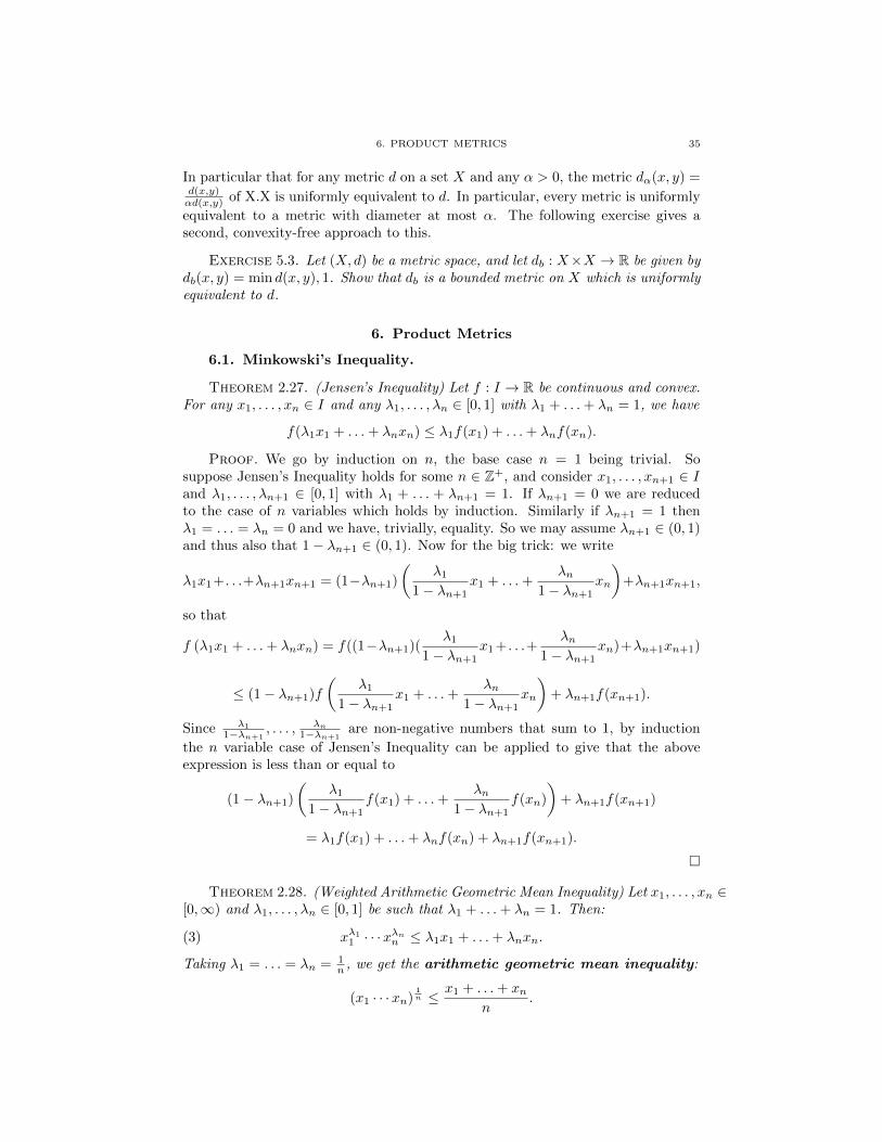
6. PRODUCT METRICS 35

In particular that for any metric d on a set X and any α > 0, the metric dα(x, y) =d(x,y)αd(x,y) of X.X is uniformly equivalent to d. In particular, every metric is uniformly

equivalent to a metric with diameter at most α. The following exercise gives asecond, convexity-free approach to this.

Exercise 5.3. Let (X, d) be a metric space, and let db : X×X → R be given bydb(x, y) = min d(x, y), 1. Show that db is a bounded metric on X which is uniformlyequivalent to d.

6. Product Metrics

6.1. Minkowski’s Inequality.

Theorem 2.27. (Jensen’s Inequality) Let f : I → R be continuous and convex.For any x1, . . . , xn ∈ I and any λ1, . . . , λn ∈ [0, 1] with λ1 + . . .+ λn = 1, we have

f(λ1x1 + . . .+ λnxn) ≤ λ1f(x1) + . . .+ λnf(xn).

Proof. We go by induction on n, the base case n = 1 being trivial. Sosuppose Jensen’s Inequality holds for some n ∈ Z+, and consider x1, . . . , xn+1 ∈ Iand λ1, . . . , λn+1 ∈ [0, 1] with λ1 + . . . + λn+1 = 1. If λn+1 = 0 we are reducedto the case of n variables which holds by induction. Similarly if λn+1 = 1 thenλ1 = . . . = λn = 0 and we have, trivially, equality. So we may assume λn+1 ∈ (0, 1)and thus also that 1− λn+1 ∈ (0, 1). Now for the big trick: we write

λ1x1+. . .+λn+1xn+1 = (1−λn+1)

(λ1

1− λn+1x1 + . . .+

λn1− λn+1

xn

)+λn+1xn+1,

so that

f (λ1x1 + . . .+ λnxn) = f((1−λn+1)(λ1

1− λn+1x1 + . . .+

λn1− λn+1

xn)+λn+1xn+1)

≤ (1− λn+1)f

(λ1

1− λn+1x1 + . . .+

λn1− λn+1

xn

)+ λn+1f(xn+1).

Since λ1

1−λn+1, . . . , λn

1−λn+1are non-negative numbers that sum to 1, by induction

the n variable case of Jensen’s Inequality can be applied to give that the aboveexpression is less than or equal to

(1− λn+1)

(λ1

1− λn+1f(x1) + . . .+

λn1− λn+1

f(xn)

)+ λn+1f(xn+1)

= λ1f(x1) + . . .+ λnf(xn) + λn+1f(xn+1).

�

Theorem 2.28. (Weighted Arithmetic Geometric Mean Inequality) Let x1, . . . , xn ∈[0,∞) and λ1, . . . , λn ∈ [0, 1] be such that λ1 + . . .+ λn = 1. Then:

(3) xλ11 · · ·xλnn ≤ λ1x1 + . . .+ λnxn.

Taking λ1 = . . . = λn = 1n , we get the arithmetic geometric mean inequality:

(x1 · · ·xn)1n ≤ x1 + . . .+ xn

n.

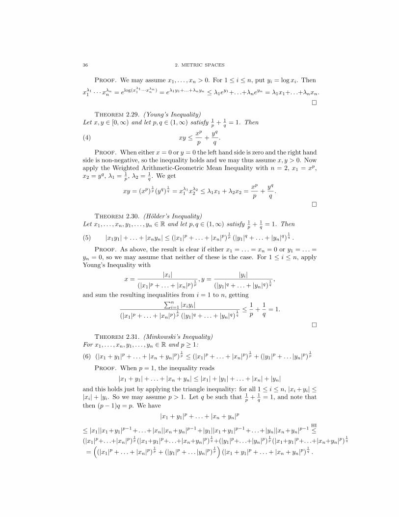
36 2. METRIC SPACES

Proof. We may assume x1, . . . , xn > 0. For 1 ≤ i ≤ n, put yi = log xi. Then

xλ11 · · ·xλnn = elog(x

λ11 ···x

λnn ) = eλ1y1+...+λnyn ≤ λ1e

y1+. . .+λneyn = λ1x1+. . .+λnxn.

�

Theorem 2.29. (Young’s Inequality)Let x, y ∈ [0,∞) and let p, q ∈ (1,∞) satisfy 1

p + 1q = 1. Then

(4) xy ≤ xp

p+yq

q.

Proof. When either x = 0 or y = 0 the left hand side is zero and the right handside is non-negative, so the inequality holds and we may thus assume x, y > 0. Nowapply the Weighted Arithmetic-Geometric Mean Inequality with n = 2, x1 = xp,x2 = yq, λ1 = 1

p , λ2 = 1q . We get

xy = (xp)1p (yq)

1q = xλ1

1 xλ22 ≤ λ1x1 + λ2x2 =

xp

p+yq

q.

�

Theorem 2.30. (Holder’s Inequality)Let x1, . . . , xn, y1, . . . , yn ∈ R and let p, q ∈ (1,∞) satisfy 1

p + 1q = 1. Then

(5) |x1y1|+ . . .+ |xnyn| ≤ (|x1|p + . . .+ |xn|p)1p (|y1|q + . . .+ |yn|q)

1q .

Proof. As above, the result is clear if either x1 = . . . = xn = 0 or y1 = . . . =yn = 0, so we may assume that neither of these is the case. For 1 ≤ i ≤ n, applyYoung’s Inequality with

x =|xi|

(|x1|p + . . .+ |xn|p)1p

, y =|yi|

(|y1|q + . . .+ |yn|q)1q

,

and sum the resulting inequalities from i = 1 to n, getting∑ni=1 |xiyi|

(|x1|p + . . .+ |xn|p)1p (|y1|q + . . .+ |yn|q)

1q

≤ 1

p+

1

q= 1.

�

Theorem 2.31. (Minkowski’s Inequality)For x1, . . . , xn, y1, . . . , yn ∈ R and p ≥ 1:

(6) (|x1 + y1|p + . . .+ |xn + yn|p)1p ≤ (|x1|p + . . .+ |xn|p)

1p + (|y1|p + . . . |yn|p)

1p

Proof. When p = 1, the inequality reads

|x1 + y1|+ . . .+ |xn + yn| ≤ |x1|+ |y1|+ . . .+ |xn|+ |yn|and this holds just by applying the triangle inequality: for all 1 ≤ i ≤ n, |xi+yi| ≤|xi| + |yi. So we may assume p > 1. Let q be such that 1

p + 1q = 1, and note that

then (p− 1)q = p. We have

|x1 + y1|p + . . .+ |xn + yn|p

≤ |x1||x1 +y1|p−1 + . . .+ |xn||xn+yn|p−1 + |y1||x1 +y1|p−1 + . . .+ |yn||xn+yn|p−1HI≤

(|x1|p+. . .+|xn|p)1p (|x1+y1|p+. . .+|xn+yn|p)

1q +(|y1|p+. . .+|yn|p)

1p (|x1+y1|p+. . .+|xn+yn|p)

1q

=(

(|x1|p + . . .+ |xn|p)1p + (|y1|p + . . . |yn|p)

1p

)(|x1 + y1|p + . . .+ |xn + yn|p)

1q .

Dividing both sides by (|x1 + y1|p + . . .+ |xn + yn|p)1q and using 1− 1

q = 1p , we get

the desired result. �

For p ∈ [1,∞) and x ∈ RN , we put

||x||p =

(N∑i=1

|xi|p)

anddp : RN × RN → R, dp(x, y) = ||x− y||p.

We also put||x||∞ = max

1≤i≤N|xi|

andd∞ : RN × RN → R, d∞(x, y) = ||x− y||∞.

Lemma 2.32. a) For each fixed nonzero x ∈ RN , the function p 7→ ||x||p isdecreasing and limp→∞ ||x||p = ||x||∞.b) For all 1 ≤ p ≤ ∞ and x ∈ RN we have

||x||∞ ≤ ||x||p ≤ ||x||1 = |x1|+ . . .+ |xN | ≤ N ||x||∞.

Proof. a) Let 1 ≤ p ≤ p′ < ∞, and let 0 6= x = (x1, . . . , xN ) ∈ RN . For anyα ≥ 0 we have ||αx||p = |α|||x||p, so we are allowed to rescale: put y = ( 1

||x||p′)x,

so ||y||p′ ≤ 1. Then |yi| ≤ 1 for all i, so |yi|p′ ≤ |yi|p for all i, so ||y||p ≥ 1 and thus

||x||p ≥ ||x||p′ .Similarly, by scaling we reduce to the case in which the maximum of the |xi|’s

is equal to 1. Then in limp→∞ |x1|p+ . . .+ |xN |p, all of the terms |xi|p with |xi| < 1converge to 0 as p→∞; the others converge to 1; so the given limit is the numberof terms with absolute value 1, which lies between 1 and N : that is, it is always atleast one and it is bounded independently of p. Raising this to the 1/p power andtaking the limit we get 1.b) The inequalities ||x||∞ ≤ ||x||p ≤ ||x||1 follow from part a). For the latterinequality, let x = (x1, . . . , xN ) ∈ RN and suppose that i is such that |xi| =max1≤i≤N |xi|. Then

|x1|+ . . .+ |xN | ≤ |xi|+ . . . |xi| = N ||x||∞. �

Theorem 2.33. For each p ∈ [1,∞), dp is a metric on RN , and all of thesemetrics are Lipschitz equivalent.

Proof. For any 1 ≤ p ≤ ∞ and x, y, z ∈ RN , Minkowski’s Inequality gives

dp(x, z) = ||x−z||p = ||(x−y)+(y−z)||p ≤ ||x−y||p+||y−z||p = dp(x, y)+dp(x, z).

Thus dp satisfies the triangle inequality; that dp(x, y) = dp(y, x) and dp(x, y) =0 ⇐⇒ x = y is immediate. So each dp is a metric on RN . Lemma 2.32 shows thatfor all 1 ≤ p ≤ ∞, dp is Lipschitz equivalent to d∞. Since Lipschitz equivalenceis indeed an equivalence relation, this implies that all the metrics dp are Lipschitzequivalent. �

The metric d2 on RN is called the Euclidean metric. The topology that itgenerates is called the Euclidean topology. The point of the above discussion isthat all metrics dp are close enough to the Euclidean metric so as to generate theEuclidean topology.

38 2. METRIC SPACES

6.2. Product Metrics.

Let (Xi, di)i∈I be an indexed family of metric spaces. Our task is to put a metricon the Cartesian product X =

∏i∈I Xi. Well, but that can’t be right: we have

already put some metric on an arbitrary set, namely the discrete metric. Ratherwe want to put a metric on the product which usefully incorporates the metrics onthe factors, in a way which generalizes the metrics dp on RN .

This is still not precise enough. We are lingering over this point a bit to emphasizethe fundamental perspective of general topological spaces that we currently lack:eventually we will discuss the product topology, which is a canonically definedtopology on any Cartesian product of topological spaces. With this perspective, theproblem can then be gracefully phrased as that of finding a metric on a Cartesianproduct of metric spaces that induces the product topology. For now we bring outagain our most treasured tool: sequences. Namely, convergence in the Euclideanmetric on RN has the fundamental property that a sequence x in RN converges ifffor all 1 ≤ i ≤ N , its ith component sequence x(i) converges in R.

In general, let us say that a metric on X =∏i∈I Xi is good if for any sequence

x in X and point x ∈ X, we have x → x in X iff for all i ∈ I, the componentsequence x(i) converges to the ith component x(i) of x.

In the case of finite products, we have already done almost all of the work.

Lemma 2.34. For 1 ≤ i ≤ N , let {x(i)n } be a sequence of non-negative real

numbers, and for n ∈ Z+ let mn = max1≤i≤N x(i)n . Then mn → 0 ⇐⇒ x

(i)n → 0

for all 1 ≤ i ≤ N .


Theorem 2.35. Let (X1, d1), . . . , (XN , dN ) be a finite sequence of metric spaces,

and put X =∏Ni=1Xi. Fix p ∈ [1,∞], and consider the function

dp : X ×X → R, dp((x1, . . . , xN ), (y1, . . . , yN )) =

(N∑i=1

|di(xi, yi)|p) 1p

.

a) The function dp is a metric function on X.b) For p, p′ ∈ [1,∞], the metrics dp and dp′ are Lipschitz equivalent.c) The function dp is a good metric on X.

Proof. Notice first that if each Xi is equal to R with the standard Euclideanmetric, then parts a) and b) reduce to Theorem 2.33 and part c) is a familiar(and easy) fact from basic real analysis: a sequence in RN converges iff each of itscomponent sequences converge. The proofs of parts a) and b) in the general caseare almost identical and are left to the reader as a straightforward but importantexercise.

In view of part b), it suffices to establish part c) for any one value of p, andthe easiest is probably p = ∞, since d∞(x, y) = maxi di(xi, yi). If x is a sequencein X and x is a point of X, we are trying to show that

d∞(xn, x) = max di(x(i)n , x(i))→ 0 ⇐⇒ ∀1 ≤ i ≤ N, di(x(i)

n , x(i))→ 0.

This follows from Lemma 2.34. �

For infinite families of metric spaces, things get more interesting. The following isa variant of [Du, Thm. IX.7.2].

Theorem 2.36. Let I be an infinite set, let (Xi, di)i∈I be an indexed family ofmetric spaces, let X =

∏i∈I Xi, and let

d : X ×X → [0,∞], d(x, y) = supi∈I

di(xi, yi).

a) If there is a finite subset J ⊂ I and D < ∞ such that for all i ∈ I \ J we havediamXi ≤ D, then d is a metric on X.b) The following are equivalent:(i) d is a good metric.(ii) For all δ > 0, {i ∈ I | diamXi ≥ δ} is finite.

Proof. �

Corollary 2.37. Let {Xn, dn}∞n=1 be an infinite sequence of metric spaces.Then there is a good metric on the Cartesian product X =

∏∞i=1Xn.

Proof. The idea is simple: the given sequence of metrics need not satisfy thehypotheses of Theorem 2.36 – e.g. they will not if each Xn has infinite diameter– but we can replace each dn with a topologically equivalent metric so that thehypotheses hold. Indeed, the metric d′n = dn

2n(dn+1 is topologically equivalent and

has diameter at most 12n . The family (Xn, d

′n) satisfies the hypotheses of Theorem

2.36b), so d = supn d′n is a good metric on X. �

Notice that Corollary 2.37 in particular shows that∏∞i=1 R and

∏∞i=1[a, b] can be

given metrics so that convergence amounts to convergence in each factor. Theseare highly interesting and important examples in the further study of analysis andtopology. The latter space is often called the Hilbert cube.

There is a case left over: what happens when we have a family of metrics in-dexed by an uncountable set I? In this case the condition that all but finitelymany factors have diameter less than any given positive constant turns out to beprohibitively strict.

Exercise 6.2. Let {Xi, di}i∈I be a family of metrics indexed by an uncount-able set I. Suppose that diamXi > 0 for uncountably many i ∈ I – equivalently,uncountably many Xi contains more than one point. Show that there is δ > 0 suchthat {i ∈ I | diamXi ≥ δ} is uncountable.

Thus Theorem 2.37 can never be used to put a good metric on an uncountableproduct except in the trivial case that all but countably many of the spaces Xi

consist of a single point. (Nothing is gained by taking Cartesian products withone-point sets: this is the multiplicative equivalent of repeatedly adding zero!) Atthe moment this seems like a weakness of the result. Later we will see that is isessential: the Cartesian product of an uncountable family of metric spaces eachconsisting of more than a single point cannot in fact be given any good metric. Inlater terminology, this is an instance of nonmetrizability of large Cartesian products.

40 2. METRIC SPACES


Exercise 6.3. Let X and Y be metric spaces, and let X × Y be endowed withany good metric. Let f : X → Y be a function.a) Show that if f is continuous, its graph G(f) = {(x, f(x) | x inX} is a closedsubset of X × Y .b) Give an example of a function f : [0,∞) → [0,∞) which is discontinuous at 0but for which G(f) is closed in [0,∞)× [0,∞).

7. Compactness

7.1. Basic Properties of Compactness.

Let X be a metric space. For a subset A ⊂ X, a family {Yi}i∈I of subsets ofX is a covering of A if A ⊂

⋃i∈I Yi. A subset A ⊂ X is compact if for every

open covering {Ui}i∈I of A there is a finite subset J ⊂ I such that {Ui}i∈J coversA.

Exercise 7.1. Show (directly) that A = {0} ∪ { 1n}∞n=1 ⊂ R is compact.

Exercise 7.2. Let X be a metric space, and let A ⊂ X be a finite subset. Showthat A is compact.

Lemma 2.38. Let X be a metric space, and let K ⊂ Y ⊂ X. Then K iscompact as a subset of Y if and only if K is compact as a subset of X.

Proof. Suppose K is compact as a subset of Y , and let {Ui}i∈I be a familyof open subsets of X such that K ⊂

⋃i∈I Ui. Then {Ui ∩ Y }i∈I is a covering of

K by open subsets of Y , and since K is compact as a subset of Y , there is a finitesubset J ⊂ I such that K ⊂

⋃i∈J Ui ∩ Y ⊂

⋃i∈J Ui.

Suppose K is compact as a subset of X, and let {Vi}i∈I be a family of opensubsets of Y such that K ⊂

⋃i∈I Vi. By X.X we may write Vi = Ui ∩ Y for some

open subset of X. Then K ⊂⋃i∈I Vi ⊂

⋃i∈I Ui, so there is a finite subset J ⊂ I

such that K ⊂⋃i∈J Ui. Intersecting with Y gives

K = K ∩ Y ⊂

(⋃i∈J

Ui

)∩ Y =

⋃i∈J

Vi. �

A sequence {An}∞n=1 of subsets of X is expanding if An ⊂ An+1 for all n ≥ 1.We say the sequence is properly expanding if An ( An+1 for all n ≥ 1. Anexpanding open cover is an expanding sequence of open subsets with X =⋃∞n=1Ai; we define a properly expanding open covering similarly.

Exercise 7.3. Let {An}∞n=1 be a properly expanding open covering of X.a) Let J ⊂ Z+ be finite, with largest element N . Show that

⋃i∈J Ai = AN .

b) Suppose that an expanding open covering {An}∞n=1 admits a finite subcovering.Show that there is N ∈ Z+ such that X = AN .c) Show that a properly expanding open covering has no finite subcovering, and thusif X admits a properly expanding open covering it is not compact.

An open covering {Ui}i∈I is disjoint if for all i 6= j, Ui ∩ Uj = ∅.

Exercise 7.4. a) Let {Ui}i∈I be a disjoint open covering of X. Show that thecovering admits no proper subcovering.

7. COMPACTNESS 41

b) Show: if X admits an infinite disjoint open covering, it is not compact.c) Show: a discrete space is compact iff it is finite.

Any property of a metric space formulated in terms of open sets may, by takingcomplements, also be formulated in terms of closed sets. Doing this for compactnesswe get the following simple but useful criterion.

Proposition 2.39. For a metric space X, the following are equivalent:(i) X is compact.(ii) X satisfies the finite intersection property: if {Ai}i∈I is a family of closedsubsets of X such that for all finite subsets J ⊂ I we have

⋂i∈J Ai 6= ∅, then⋂

i∈I Ai 6= ∅.


Another easy but crucial observation is that compactness is somehow antitheticalto discreteness. More precisely, we have the following result.

Proposition 2.40. For a metric space X, the following are equivalent:(i) X is both compact and topologically discrete.(ii) X is finite.


Lemma 2.41. Let X be a metric space and A ⊂ X.a) If X is compact and A is closed in X, then A is compact.b) If A is compact, then A is closed in X.c) If X is compact, then X is bounded.

Proof. a) Let {Ui}i∈I be a family of open subsets of X which covers A: i.e.,A ⊂

⋃i∈I Ui. Then the family {Ui}i∈I ∪ {X \ A} is an open covering of X. Since

X is compact, there is a finite subset J ⊂ I such that X =⋃i∈J Ui ∪ (X \A), and

it follows that A ⊂⋃i∈J Ui.

b) Let U = X \ A. For each p ∈ U and q ∈ A, let Vq = B(p, d(p,q)2 ) and Wq =

B(p, d(p,q)2 ), so Vq∩Wq = ∅. Moreover, {Wq}q∈A is an open covering of the compact

set A, so there are finitely many points q1, . . . , qn ∈ A such that

A ⊂n⋃i=1

Wi =: W,

say. Put V =⋂ni=1 Vi. Then V is a neighborhood of p which does not intersect W ,

hence lies in X \A = U . This shows that U = X \A is open, so A is closed.c) Let x ∈ X. Then {B◦(x, n)}∞n=1 is an expanding open covering of X; since X iscompact, we have a finite subcovering. By Exercise 2, we have X = B◦(x,N) forsome N ∈ Z+, and thus X is bounded. �

Example 7.1. Let X = [0, 10] ∩ Q be the set of rational points on the unitinterval. As a subset of itself, X is closed and bounded. For n ∈ Z+, let

Un = {x ∈ X | d(x,√

2) >1

n}.

Then {Un}∞n=1 is a properly expanding open covering of X, so X is not compact.

Proposition 2.42. Let f : X → Y be a surjective continuous map of topolog-ical spaces. If X is compact, so is Y .

42 2. METRIC SPACES

Proof. Let {Vi}i∈I be an open cover of Y . For i ∈ I, put Ui = f−1(Vi). Then{Ui}i∈I is an open cover of X. Since X is compact, there is a finite J ⊂ I suchthat

⋃i∈J Ui = X, and then Y = f(X) = f(

⋃i∈J Ui) =

⋃i∈J f(Ui) =

⋃i∈J Vi. �

Theorem 2.43. (Extreme Value Theorem) Let X be a compact metric space. Acontinuous function f : X → R is bounded and attains its maximum and minimum:there are xm, xM ∈ X such that for all x ∈ X, f(xm) ≤ f(x) ≤ f(xM ).

Proof. Since f(X) ⊂ R is compact, it is closed and bounded. Thus inf f(X)is a finite limit point of f(X), so it is the minimum; similarly sup f(X) is themaximum. �

7.2. Heine-Borel.

When one meets a new metric space X, it is natural to ask: which subsets Aof X are compact? Lemma 2.41 gives the necessary condition that A must beclosed and bounded. In an arbitrary metric space this is nowhere near sufficient,and one need look no farther than an infinite set endowed with the discrete metric:every subset is closed and bounded, but the only compact subsets are the finitesubsets. In fact, compactness is a topological property whereas we saw in §6 thatgiven any metric space there is a topologically equivalent bounded metric.

Nevertheless in some metric spaces it is indeed the case that every closed, boundedset is compact. In this section we give a concrete treatment that Euclidean spaceRN has this property: this is meant to be a reminder of certain ideas from honorscalculus / elementary real analysis that we will shortly want to abstract and gen-eralize.

A sequence {An}∞n=1 of subsets of X is nested if An+1 ⊃ An for all n ≥ 1.

Let a1 ≤ b1, a2 ≤ b2, . . . , an ≤ bn be real numbers. We put

n∏i=1

[ai, bi] = {x = (x1, . . . , xn) ∈ Rn | ∀1 ≤ i ≤ n, ai ≤ xi ≤ bi}.

We will call such sets closed boxes.

Exercise 7.7.a) Show: a subset A ⊂ Rn is bounded iff it is contained in some closed box.b) Show that

diam

(n∏i=1

[ai, bi]

)=

√√√√ n∑i=1

(ai − bi)2.

Lemma 2.44. (Lion-Hunting Lemma) Let {Bm}∞m=1 be a nested sequence ofclosed boxes in Rn. Then there is x ∈

⋂∞m=1 Bm.

b) If limm→∞ diamBm = 0, then⋂∞m=1 Bm consists of a single point.

Proof. Write Bm =∏ni=1[ai(m), bi(m)]. Since the sequence is nested, we have

ai(m) ≤ ai(m+ 1) ≤ bi(m+ 1) ≤ bi(m)

7. COMPACTNESS 43

for all i and m. Then xm = (xm(1), . . . , xm(n)) ∈⋂∞m=1 Bm iff for all 1 ≤ i ≤ n we

have am(i)) ≤ xm ≤ bm(i). For 1 ≤ i ≤ n, put

Ai = supmam(i), Bi = inf

mbm(i).

It then follows that∞⋂m=1

Bm =

n∏i=1

[Ai, Bi],

which is nonempty. �

Exercise 7.8. In the above proof it is implicit that Ai ≤ Bi for all 1 ≤ i ≤ n.Convince yourself that you could write down a careful proof of this (e.g. by writingdown a careful proof!).

Exercise 7.9. Under the hypotheses of the Lion-Hunting Lemma, show thatthe following are equivalent:(i) inf{diamBm}∞m=1 = 0.(ii)

⋂∞m=1 Bm consists of a single point.

Theorem 2.45. (Heine-Borel) Every closed, bounded subset A ⊂ Rn is com-pact.

Proof. Because every closed bounded subset is a subset of a closed box andclosed subsets of compact sets are compact, it is sufficient to show the compactnessof every closed box B =

∏ni=1[ai, bi]. Let U = {Ui}i∈I be an open covering of B.

Seeking a contradiction we suppose U admits no finite subcovering. We bisectB into 2n closed subboxes of equal size, so that e.g. the bottom leftmost one is∏ni=1[ai,

ai+bi2 ]. It must be that at least one of the subboxes cannot be covered by

any finite number of sets in U : if all 2n of them have finite subcoverings, takingthe union of 2n finite subcoverings, we get a finite subcovering of B. Identify onesuch subbox B1, and notice that diamB1 = 1

2 diamB. Now bisect B1 and repeatthe argument: we get a nested sequence {Bm}∞m=1 of closed boxes with

diamBm =diamB

2m.

By the Lion-Hunting Lemma there is x ∈⋂∞m=1 Bm.2 Choose U0 ∈ U such that

x ∈ U0. Since U0 is open, for some ε > 0 we have

x ∈ B◦(x, ε) ⊂ U0.

For sufficiently large m we have – formally, by the Archimedean property of R –that diamBm < ε. Thus every point in Bm has distance less than ε from x so

Bm ⊂ B◦(x, ε) ⊂ U0.

This contradicts the heck out of the fact that Bm admits no finite subcovering. �

Proposition 2.46. Let X be a compact metric space, and let A ⊂ X be aninfinite subset. Then A has a limit point in X.

2Though we don’t need it, it follows from Exercise 1.9 that the intersection point x is unique.

44 2. METRIC SPACES

Proof. Seeking a contradiction we suppose that A has no limit point in X.Then also no subset A′ ⊂ A has any limit points in X. Since a set is closed if itcontains all of its limit points, every subset of A is closed in X. In particular A isclosed in X, hence A is compact. But since for all x ∈ A, A \ {x} is closed in A, wehave that{x} is open in A. (In other words, A is discrete.) Thus {{x}}x∈A is aninfinite cover of A without a finite subcover, so A is not compact: contradiction. �

Theorem 2.47. (Bolzano-Weierstrass for Sequences) Every bounded sequencein RN admits a convergent subsequence.

Proof. Step 1: Let N = 1. I leave it to you to carry over the proof of Bolzano-Weierstrass in R given in § 2.2 to our current sequential situation: replacing theMonotonicity Lemma with the Rising Sun Lemma, the endgame is almost identical.Step 2: Let N ≥ 2, and let {xn}∞n=1 be a bounded sequence in RN . Then eachcoordinate sequence {xn(i)}∞n=1is bounded, so Step 1 applies to each of them.

However, if we just extract subsequences for each component separately, wewill have N different subsequences, and it will in general not be possible to get onesubsequence out of all of them. So we proceed in order: first we extract a subse-quence such that the first coordinates converge. Then we extract a subsequenceof the subsequence such that the second coordinates converge. This does not dis-turb what we’ve already done, since every subsequence of a convergent sequence isconvergent (we’re applying this in the familiar context of real sequences, but it isequally true in any metric space). Thus we extract a sub-sub-sub...subsequence (N“subs” altogether) which converges in every coordinate and thus converges. But asub-sub....subsequence is just a subsequence, so we’re done. �

A metric space is sequentially compact if every sequence admits a convergentsubsequence.

A metric space X is limit point compact if every infinite subset A ⊂ X hasa limit point in X.

8. Completeness

8.1. Lion Hunting In a Metric Space.

Recall the Lion-Hunting Lemma: any nested sequence of closed boxes in RN has acommon intersection point; if the diameters approach zero, then there is a uniqueintersection point. This was the key to the proof of the Heine-Borel Theorem.

Suppose we want to hunt lions in an arbitrary metric space: what should we replace“closed box” with? The following exercise shows that we should at least keep the“closed” part in order to get something interesting.

Exercise 8.1. Find a nested sequence A1 ⊃ A2 ⊃ . . . ⊃ An . . . of nonemptysubsets of [0, 1] with

⋂∞n=1Ai = ∅.

So perhaps we should replace “closed box” with “closed subset”? Well...we could.However, even in R, if we replace “closed box” with “closed set”, then lion huntingneed not succeed: for n ∈ Z+, let An = [n,∞). Then {An}∞n=1 is a nested sequenceof closed subsets with

⋂∞n=1An = ∅.

8. COMPLETENESS 45

Suppose however that we consider nested covers of nonempty closed subsets withthe additional property that diamAn → 0. In particular, all but finitely many An’sare bounded, so the previous problem is solved. Indeed, Lion-Hunting works underthese hypothesis in RN because of Heine-Borel: some An is closed and bounded,hence compact, so we revisit the previous case.

A metric space is complete if for every nested sequence {An} of nonempty closedsubsets with diameter tending to 0 we have

⋂nAn 6= ∅.

The following result shows that completeness, like compactness, is a kind of in-trinsic closedness property.

Lemma 2.48. Let Y be a subset of a metric space X.a) If X is complete and Y is closed, then Y is complete.b) If Y is complete, then Y is closed.

Proof. a) If Y is closed in X, then a nested sequence {An}∞n=1 of nonemptyclosed subsets of Y with diameter approaching 0 is also a nested sequence ofnonempty closed subsets of X with diameter approaching 0. Since X is complete,there is x ∈

⋂nAn.

b) If Y is not closed, let y be a sequence in Y converging to an element x ∈ X \ Y .Put An = {yk | k ≥ n}. Then {An}∞n=1 is a nested sequence of nonempty closedsubsets of Y of diameter approaching 0 and with empty intersection. �

8.2. Cauchy Sequences.

Our Lion Hunting definition of completeness is conceptually pleasant, but it seemslike it could be a lot of work to check in practice. It is also – we now admit – notthe standard one. We now make the transition to the standard definition.

The proof of (ii) =⇒ (i) in Theorem X.X suggests that it would be sufficientto lion hunt using nested sequences of closed balls. This is not hard to show.

Lemma 2.49. A metric space in which each sequence of closed balls with diam-eters tending to zero has nonempty intersection is complete.

Proof. Let {An}∞n=1 be a nested sequence of nonempty closed subsets withdiameter tending to zero. We may assume without loss of generality that each Anhas finite diameter, and we may choose for all n ∈ Z+, xn ∈ An and a positivereal number rn such that An ⊂ B•(xn, rn) and rn → 0. By assumption, there is aunique point x ∈

⋂nB•(xn, rn). Then xn → x. Fix n ∈ Z+. Then x is the limit of

the sequence xn, xn+1, . . . in An, and since An is closed, x ∈ An. �

Let us nail down which sequences of closed balls we can use for lion hunting.

Lemma 2.50. Let {B•(xn, rn)}∞n=1 be a nested sequence of closed balls in ametric space X with rn → 0. Then for all ε > 0, there is N = N(ε) such that forall m,n ≥ N , d(xm, xn) ≤ ε.

Proof. Fix ε > 0, and choose N such that rN ≤ ε2 . Then if m,n ≥ N we have

xn, xm ∈ B•(xN , rN ), so d(xn, xm) ≤ 2rN ≤ ε. �

46 2. METRIC SPACES

At last, we have motivated the following definition. A sequence {xn} in am metricspace X is Cauchy if for all ε > 0, there is N = N(ε) such that for all m,n ≥ N ,d(xm, xn) < ε. Thus in a nested sequence of closed balls with diameter tending tozero, the centers of the balls form a Cauchy sequence. Moreover:

Lemma 2.51. Let {xn} be a sequence in a metric space X, and for n ∈ Z+ putAn = {xk | k ≥ n}. The following are equivalent:(i) The sequence {xn} is Cauchy.(ii) limn→∞ diamAn = 0.


Exercise 8.3. Show that every convergent sequence is Cauchy.

Lemma 2.52. Every partial limit of a Cauchy sequence is a limit.

Proof. Let {xn} be a Cauchy sequence, and let x ∈ X be such that somesubsequence xnk → x. Fix ε > 0, and choose N such that for all m,n ≥ N ,d(xm, xn) < ε

2 . Choose K such that nK ≥ N and for all k ≥ K, d(xnk , x) < ε2 .

Then for all n ≥ N ,

d(xn, x) ≤ d(xn, xnK ) + d(xnK , x) <ε

2+ε

2= ε. �

Proposition 2.53. For a metric space X, the following are equivalent:(i) X is complete.(ii) Every Cauchy sequence in X is convergent.

Proof. ¬ (ii) =⇒ ¬ (i): Suppose {xn} is a Cauchy sequence which doesnot converge. By Lemma 2.52, the sequence {xn} has no partial limit, so An ={xk | k ≥ n} is a nested sequence of closed subsets with diameter tending to 0and

⋂nAn = ∅, so X is not complete. (ii) =⇒ (i): By Lemma 2.49, it is

enough to show that any nested sequence of closed balls with diameters tending tozero has nonempty intersection. By Lemma 2.50, the sequence of centers {xn} isCauchy, hence converge to x ∈ X by assumption. For each n ∈ Z+, the sequencexn, xn+1, . . . lies in B•(xn, rn), hence the limit, x, lies in B•(xn, rn). �

8.3. Baire’s Theorem.

A subset A of a metric space X is nowhere dense if A contains no nonempty

open subset, or in other words if A◦

= ∅.

Exercise 8.4. Let x be a point of a metric space X. Show that x is a limitpoint of X iff {x} is nowhere dense.

Theorem 2.54. (Baire) Let X be a complete metric space.a) Let {Un}∞n=1 be a sequence of dense open subsets of X. Then U =

⋂∞n=1 Un is

also dense in X.b) Let {An}∞n=1 be a countable collection of nowhere dense subsets of X. ThenA =

⋃∞n=1An has empty interior.

Proof. a) We must show that for every nonempty open subset W of X wehave W ∩ U 6= ∅. Since U1 is open and dense, W ∩ U1 is nonempty and openand thus contains some closed ball B•(x1, r1) with 0 < r1 ≤ 1. For n ≥ 1, havingchosen xn and rn ≤ 1

n , since Un+1 is open and dense, B(xn, rn)∩Un+1 is nonempty

8. COMPLETENESS 47

and open and thus contains some closed ball B•(xn+1, rn+1) with 0 < rn+1 ≤ 1n+1 .

Since X is complete, there is a (unique)

x ∈∞⋂n=2

B•(xn, rn) ⊂∞⋂n=1

B(xn, rn) ∩ Un ⊂∞⋂n=1

Un = U.

Moreover

x ∈ B•(x1, r1) ⊂W ∩ U1 ⊂W,so

x ∈ U ∩W.b) Without loss of generality we may assume that each An is closed, because Anis nowhere dense iff An is nowhere dense, and a subset of a nowhere dense set iscertainly nowhere dense. For n ∈ Z+, let Un = X \An. Each Un is open; moreover,since An contains no nonempty open subset, every nonempty open subset mustintersect Un and thus Un is dense. By part a),

⋂∞n=1 Un =

⋂∞n=1X \ An = X \ A

is dense. Again, this means that every nonempty open subset of X meets thecomplement of A so no nonempty open subset of X is contained in A. �

Corollary 2.55. Let X be a nonempty complete metric space in which everypoint is a limit point. Then X is uncountable.

Proof. Let A = {an | n ∈ Z+} be a countably infinite subset of X. Then each{an} is nowhere dense, so by Theorem 2.54, A =

⋃∞n=1{an} has empty interior. In

particular, A ( X. �

Observe that Corollary 2.55 applies to R and gives a purely topological proof of itsuncountability!

Corollary 2.56. A countably infinite complete metric space has infinitelymany isolated points.

Proof. Let X be a complete metric space with only finitely many isolatedpoints, say A = {a1, . . . , an}. We will show that X is uncountable. Let Y = X \A,let y ∈ Y , and let V be an open neighborhood of y in Y , so V = U∩Y for some openneighborhood of y in X. By definition of Y , V is infinite. However, intersectingwith Y only involves removing finitely many points, so V must also be infinite! Itfollows that every point of the metric space Y is a limit point. As in any metricspace, the subset of all isolated points is open, so its complement Y is closed inthe complete space X, so it too is complete. Thus by Corollary 2.55 Y must beuncountably infinite, hence so is X. �

One interesting consequence of these results is that we can deduce purely topologicalconsequences of the metric condition of completeness.

Example 8.1. Let Q be the rational numbers, equipped with the usual Euclideanmetric d(x, y) = |x − y|. As we well know, (Q, d) is not complete. But here is amore profound question: is there some topologically equivalent metric d′ on Q whichis complete? Now in general a complete metric can be topologically equivalent toan incomplete metric: e.g. this happens on R. But that does not happen here: anytopologically equivalent metric is a metric on a countable set in which no point isisolated (the key observation being that the latter depends only on the topology), soby Corollary 2.55 cannot be complete.

48 2. METRIC SPACES

This example motivates the following definition: a metric space (X, d) is topo-logically complete if there is a complete metric d′ on X which is topologicallyequivalent to d.

Exercise 8.5. Show that the space of irrational numbers R \Q (still with thestandard Euclidean metric d(x, y) = |x− y|) is topologically complete.

9. Total Boundedness

We saw above that the property of boundedness is not only not preserved by home-omorphisms of metric spaces, it is not even preserved by uniformeomorphisms ofmetric spaces (and also that it is preserved by Lipschitzeomorphisms). Though thiswas as simple as replacing any unbounded metric by the standard bounded metricdb(x, y) = min d(x, y), 1, intuitively it is still a bit strange: e.g. playing around abit with examples, one soon suspects that for subspaces of Euclidean space RN , theproperty of boundedness is preserved by uniformeomorphisms.

The answer to this puzzle lies in identifying a property of metric spaces: perhapsthe most important property that does not get “compactness level PR”.

A metric space X is totally bounded if for all ε > 0, it admits a finite cover

by open ε-balls: there is N ∈ Z+ and x1, . . . , xN ∈ X such that X =⋃Ni=1B(xi, ε).

Since any finite union of bounded sets is bounded, certainly total boundednessimplies boundedness (thank goodness).

Notice that we could require the balls to be closed without changing the defini-tion: just slightly increase or decrease ε. (And indeed, sometimes we will want touse one form of the definition and sometimes the other.) In fact we don’t reallyneed balls at all; the following is useful reformulation.

Lemma 2.57. For a metric space X, the following are equivalent:(i) For all ε > 0, there exists a finite family S1, . . . , SN of subsets of X such that

diamSi ≤ ε for all i and X =⋃Ni=1 Si.

(ii) X is totally bounded.

Proof. (i) =⇒ (ii): We may assume each Si is nonempty, and choose xi ∈ Si.Since diamSi ≤ ε, Si ⊂ B•(xi, ε) and thus X =

⋃Ni=1B

•(xi, ε).

(ii) =⇒ (i): For every ε > 0, choose x1, . . . , xN such that⋃Ni=1B

•(xi,ε2 ) = X.

We have covered X by finitely many sets each of diameter at most ε. �

Corollary 2.58.a) Every subset of a totally bounded metric space is totally bounded.b) Let f : X → Y be a uniformeomorphism of metric spaces. Then X is totallybounded iff Y is totally bounded.

Proof. a) Suppose that X is totally bounded, and let Y ⊂ X. Since X istotally bounded, for each ε > 0 there exist S1, . . . , SN ⊂ X such that diamSi < ε

for all i and X =⋃Ni=1 Si. Then diam(Si ∩ Y ) < ε for all i and Y =

⋃Ni=1(Si ∩ Y ).

b) Suppose X is totally bounded. Let ε > 0, and choose δ > 0 such that f is(ε, δ)-uniformly continuous. Since X is totally bounded there are finitely many

9. TOTAL BOUNDEDNESS 49

sets S1, . . . , SN ⊂ X with diamSi ≤ δ for all 1 ≤ i ≤ N and X =⋃Ni=1 Si. For

1 ≤ i ≤ N , let Ti = f(Si). Then diamTi ≤ ε for all i and Y =⋃Ni=1 Ti. It

follows that Y is uniformly bounded. Using the uniformly continuous functionf−1 : Y → X gives the converse implication. �

Lemma 2.59. (Archimedes) A subset of RN is bounded iff it is totally bounded.

Proof. Total boundedness always implies boundedness. Moreover any boundedsubset of RN lies in some cube Cn = [−n, n]N for some n ∈ Z+, so by Corollary2.58 it is enough to show that Cn is totally bounded. But Cn can be written as theunion of finitely many subcubes with arbitrarily small side length and thus arbi-trarily small diameter. Provide more details if you like, but this case is closed. �

Let ε > 0. An ε-net in a metric space X is a subset N ⊂ X such that for all x ∈ X,there is n ∈ N with d(x, n) < ε. An ε-packing in a metric space X is a subsetP ⊂ X such that d(p, p′) ≥ ε for all p, p′ ∈ P .

These concepts give rise to a deep duality in discrete geometry between pack-ing – namely, placing objects in a space without overlap – and covering – namely,placing objects in a space so as to cover the entire space. Notice that already wecan cover the plane with closed unit balls or we can pack the plane with closed unitballs but we cannot do both at once. The following is surely the simplest possibleduality principle along these lines.

Proposition 2.60. Let X be a metric space, and let ε > 0.a) The space X admits either a finite ε-net or an infinite ε-packing.b) If X admits a finite ε-net then it does not admit an infinite (2ε)-packing.c) Thus X is totally bounded iff for all ε > 0, there is no infinite ε-packing.

Proof. a) First suppose that we do not have a finite ε-net in X. Then Xis nonempty, so we may choose p1 ∈ X. Since X 6= B(p1, ε), there is p2 ∈ Xwith d(p1, p2) ≥ ε. Inductively, having constructed an n element ε-packing Pn ={p1, . . . , pn}, since Pn is not a finite ε-net there is pn+1 ∈ X such that d(pi, pn+1) ≥ εfor all 1 ≤ i ≤ n, so Pn+1 = Pn ∪ {pn+1} is an n + 1 element ε-packing. ThenP =

⋃n∈Z+ Pn is an infinite ε-packing.

b) Seeking a contradiction, suppose that we have both an infinite (2ε)-packing Pand a finite ε-net N . Since P is infinite, N is finite and X =

⋃n∈N B(n, ε), there

must be distinct points p 6= p′ ∈ P each lying in B(n, ε) for some n ∈ N , and thenby the triangle inequality d(p, p′) ≤ d(p, n) + d(n, p′) < 2ε.c) To say that N ⊂ X is an ε-net means precisely that if we place an open ball ofradius ε centered at each point of N , then the union of these balls covers X. Thustotal boundedness means precisely the existence of a finite ε-net for all ε > 0. Theresult then follows immediately from part a). �

Theorem 2.61. A metric space X is totally bounded iff each sequence x in Xadmits a Cauchy subsequence.

Proof. If X is not totally bounded, then by Proposition 2.60 there is aninfinite ε-packing for some ε > 0. Passing to a countably infinite subset P ={pn}∞n=1, we get a sequence such that for all m 6= n, d(pm, pn) ≥ ε. This sequencehas no Cauchy subsequence.

Now suppose that X is totally bounded, and let x be a sequence in X. By

50 2. METRIC SPACES

total boundedness, for all n ∈ Z+, we can write X as a union of finitely manyclosed subsets Y1, . . . , YN each of diameter at most 1

n (here N is of course allowedto depend on n). An application of the Pigeonhole Principle gives us a subsequenceall of whose terms lie in Yi for some i, and thus we get a subsequence each of whoseterms have distance at most ε. Unfortunately this is not quite what we want: weneed one subsequence each of whose sufficiently large terms differ by at most 1

n .We attain this via a diagonal construction: namely, let

x1,1, x1,2, . . . , x1,n, . . .

be a subsequence each of whose terms have distance at most 1. Since subspacesof totally bounded spaces are totally bounded, we can apply the argument againinside the smaller metric space Yi to get a subsubsequence

x2,1, x2,2, . . . , x2,n, . . .

each of whose terms differ by at most 12 and each x2,n is selected from the subse-

quence {x1,n}; and so on; for all m ∈ Z+ we get a subsub...subsequence

xm,1, xm,2, . . . , xm,n, . . .

each of whose terms differ by at most 1n . Now we choose the diagonal subse-

quence: put yn = xn,n for all n ∈ Z+. We allow the reader to check that this isa subsequence of the original sequence x.. This sequence satisfies d(yn, yn+k) ≤ 1

nfor all k ≥ 0, so we get a Cauchy subsequence. �

10. Separability

We remind the reader that we are an ardent fan of [Ka]. The flattery becomesespecially sincere at this point: c.f. [Ka, §5.2].

Recall that a metric space is separable if it admits a countable dense subset.

Exercise 10.1. Let f : X → Y be a continuous surjective map between metricspaces. Show that if X is separable, so is Y .

We want to compare this property with two others that we have not yet introduced.

A base B = {Bi} for the topology of a metric space X is a collection of opensubsets of X such that every open subset U of X is a union of elements of B: pre-cisely, there is a subset J ⊂ B such that

⋃i∈J Bi = U . (We remark that taking

J = ∅ we get the empty union and thus the empty set.)

The example par excellence of a base for the topology of a metric space X isto take B to be the family of all open balls in X. In this case, the fact that B is abase for the topology is in fact the very definition of the metric topology: the opensets are precisely the unions of open balls.

A countable base is just what it sounds like: a base which, as a set, is countable(either finite or countably infinite).

Proposition 2.62. a) Let X be a metric space, let B = {Bi} be a base for thetopology of X, and let Y ⊂ X be a subset. Then B ∩ Y := {Bi ∩ Y } is a base forthe topology of Y .b) If X admits a countable base, then so does all of its subsets.

10. SEPARABILITY 51

Proof. a) This follows from the fact that the open subsets of Y are preciselythose of the form U ∩ Y for U open in X. We leave the details to the reader.b) This is truly immediate. �

Theorem 2.63. For a metric space X, the following are equivalent:(i) X is separable.(ii) X admits a countable base.(iii) X is Lindelof.

Proof. (i) =⇒ (ii): Let Z be a countable dense subset. The family of openballs with center at some point of Z and radius 1

n is then also countable (becausea product of two countable sets is countable). So there is a sequence {Un}∞n=1 inwhich every such ball appears at least once. I claim that every open set of X is aunion of such balls. Indeed, let U be a nonempty subset (we are allowed to takethe empty union to get the empty set!), let p ∈ U , and let ε > 0 be such thatB(p, ε) ⊂ U . Choose n sufficiently large such that 1

n < ε2 and choose z ∈ Z such

that d(z, p) < 12n . Then p ∈ B(z, 1

n ) ⊂ B(p, ε) ⊂ U . It follows that U is a union ofballs as claimed.(ii) =⇒ (iii): Let B = {Bn}∞n=1 be a countable base for X, and let {Ui}i∈I be anopen covering of X. For each p ∈ X, we have p ∈ Ui for some i. Since Ui is a unionof elements of B and p ∈ Ui, we must have p ∈ Bn(p) ⊂ Ui for some n(p) dependingon p. Thus we have all the essential content for a countable subcovering, and weformalize this as follows: let J be the set of all positive integers n such that Bn liesin Ui for some i: notice that J is countable! For each n ∈ J , choose in ∈ I suchthat Bn ⊂ Uin . It then follows that X =

⋃n∈J Uin .

(iii) =⇒ (i): For each n ∈ Z+, the collection {B(p, 1n )}p∈X certainly covers X.

Since X is Lindelof, there is a countable subcover. Let Zn be the set of centers of theelements of this countable subcover, so Zn is a countable 1

n -net. Put Z =⋃n∈Z+ Zn.

Then Z is a countable dense subset. �

As usual, we now get to play the good properties of separability, existence of count-able bases, and Lindelofness off against one another. For instance, we get:

Corollary 2.64. a) Every subset of a separable metric space is separable.b) Every subset of a Lindelof metric space is Lindelof.c) If f : X → Y is a continuous surjective map of metric spaces and X has acountable base, so does Y .

We suggest that the reader pause and try to give a proof of Corollary 2.64 directlyfrom the definition: it is really not straightforward to do so.

Exercise 10.2. Let X be a separable metric space, and let E ⊂ X be a discretesubset: every point of E is an isolated point. Show that E is countable.

Recall that point p in a metric space is isolated if {p} is an open set. If we like,we can rephrase this by saying that p admits a neighborhood of cardinality 1. Oth-erwise p is a limit point: every neighborhood of p contains points other than p.Because finite metric spaces are discrete, we can rephrase this by saying that everyneighborhood of p is infinite. This little discussion perhaps prepares us for thefollowing more technical definition.

A point p of a metric space X is an ω-limit point if every neighborhood of pin X is uncountable.

52 2. METRIC SPACES

Theorem 2.65. A separable metric space has at most continuum cardinality.

Exercise 10.3. Prove it. (Hint: think about limits of sequences.)

Theorem 2.66. Let X be an uncountable separable metric space. Then all butcountably many points of X are ω-limit points.

Theorem 2.67. Let X be an uncountable, complete separable metric space.Then X has continuum cardinality.

Proof. By Theorem 2.65, X has at most continuum cardinality, so it willsuffice to exhibit continuum-many points of X.Step 1: We claim that for all δ > 0, there is 0 ≤ ε ≤ δ and x, y ∈ X such thatthe closed ε-balls B•(x, ε) and B•(y, ε) are disjoint and each contain uncountablymany points. Indeed, by Theorem 2.66, X has uncountably many ω-limit points.Choose two of them x 6= y and take any ε < d(x, y).Step 2: Applying the above construction with δ = 1 we get uncountable disjointclosed subsets A0 and A1 each of diameter at most 1. Each of A0 and A1 is itselfuncountable, complete and separable, so we can run the construction in A0 andin A1 to get uncountable disjoint closed subsets A0,0, A0,1 in A1 and A1,0, A1,1 inA2, each of diameter at most 1

2 . Continuing in this way we get for each n ∈ Z+ apairwise disjoint family of 2n uncountable closed subsets Ai1,...,in (with i1, . . . , in ∈{0, 1}) each of diameter at most 2−n. Any infinite binary sequence ε ∈ {0, 1}Z+

yields a nested sequence of nonempty closed subsets of diameter approaching zero,so by completeness each such sequence has a unique intersection point pε. If ε 6= ε′

are distinct binary sequences, then for some n, εn 6= ε′n, so pε and p′ε are contained

in disjoint subsets and are thus distinct. This gives 2#Z+

= #R points of X. �

The following exercise gives a subtle sharpening of Corollary ?? (which doesnot directly use Theorem 2.54).

Exercise 10.4. a) (S. Ivanov) Let X be a complete metric space without iso-lated points. Show that X has at least continuum cardinality. (Suggestion: the lackof isolated points implies that every closed ball of positive radius is infinite. Thisallows one to run the argument of Step 2 of the proof of Theorem 2.67 above.)b) Explain why the assertion that every uncountable complete metric space has atleast continuum cardinality is equivalent to the Continuum Hypothesis: i.e., thatevery uncountable set has at least continuum cardinality.3

11. Compactness Revisited

The following is perhaps the single most important theorem in metric topology.

Theorem 2.68. Let X be a metric space. The following are equivalent:(i) X is compact: every open covering of X has a finite subcovering.(ii) X is sequentially compact: every sequence in X has a convergent subsequence.(iii) X is limit point compact: every infinite subset of X has a limit point in X.(iv) X is complete and totally bounded.

3Curiously, Exercise 8 in §5.2 of [Ka] reads “Prove that every uncountable complete metricspace has at least the cardinal number c”. Is Kaplansky asking for a proof of the Continuum

Hypothesis??

11. COMPACTNESS REVISITED 53

Proof. We will show (i) =⇒ (iii) ⇐⇒ (ii) ⇐⇒ (iv) =⇒ (i).(i) =⇒ (iii): Suppose X is compact, and let A ⊂ X have no limit point in X. Wemust show that A is finite. Recall that A is obtained by adjoining the set A′ oflimit points of A, so in our case we have A = A ∪A′ = A ∪∅ = A, i.e., A is closedin the compact space X, so A is itself compact. On the other hand, no point of Ais a limit point, so A is discrete. Thus {{a}a∈A} is an open covering of A, whichcertainly has no proper subcovering: we need all the points of A to cover A! So thegiven covering must itself be finite: i.e., A is finite.(iii) =⇒ (ii): Let x be a sequence in X; we must find a convergent subsequence.If some element occurs infinitely many times in the sequence, we have a constantsubsequence, which is convergent. Otherwise A = {xn | n ∈ Z+} is infinite, so ithas a limit point x ∈ X and thus we get a subsequence of x converging to x.(ii) =⇒ (iii): Let A ⊂ X be infinite; we must show that A has a limit point in X.The infinite set A contains a countably infinite subset; enumerating these elementsgives us a sequence {an}∞n=1. By assumption, we have a subsequence converging tosome x ∈ X, and this x is a limit point of A.(ii) =⇒ (iv): Let x be a Cauchy sequence in X. By assumption x has a convergentsubsequence, which by Lemma 2.52 implies that x converges: X is complete. Letx be a sequence in X. Then x has a convergent, hence Cauchy, subsequence. ByTheorem 2.61, the space X is totally bounded.(iv) =⇒ (ii): Let x be a sequence in X. By total boundedness x admits a Cauchysubsequence, which by completeness is convergent. So X is sequentially compact.(iv) =⇒ (i): Seeking a contradiction, we suppose that there is an open covering{Ui}i∈I of X without a finite subcovering. Since X is totally bounded, it admitsa finite covering by closed balls of radius 1. It must be the case that for at leastone of these balls, say A1, the open covering {Ui ∩ A1}i∈I of A1 does not have afinite subcovering – for if each had a finite subcovering, by taking the finite unionof these finite subcoverings we would get a finite subcovering of {Ui}i∈I . Since A1

is a closed subset of a complete, totally bounded space, it is itself complete andtotally bounded. So we can cover A1 by finitely many closed balls of radius 1

2 andrun the same argument, getting at least one such ball, say A2 ⊂ A1, for which theopen covering {Ui ∩ A2}i∈I has no finite subcovering. Continuing in this way webuild a nested sequence of closed balls {An}∞n=1 of radii tending to 0, and thus alsodiamAn → 0. By completeness there is a point p ∈

⋂∞n=1An. Since

⋃i∈I Ui = X,

certainly we have p ∈ Ui for at least one i ∈ I. Since Ui is open, there is someε > 0 such that B(p, ε) ⊂ Ui. Choose N ∈ Z+ such that diamAN < ε. Then sincep ∈ AN , we have AN ⊂ B(p, ε) ⊂ Ui. But this means that AN = Ui ∩ AN is a oneelement subcovering of AN : contradiction. �

Exercise 11.1. A metric space is countably compact if every countable opencover admits a finite subcover. a) Show that for a metric space X, the followingare equivalent:(i) X is countably compact.(ii) For any sequence {An}∞n=1 of closed subsets, if for all finite nonempty subsetsJ ⊂ Z+ we have

⋂n∈J An 6= ∅, then

⋂∞n=1An 6= ∅.

(iii) For any nested sequence A1 ⊃ A2 ⊃ . . . ⊃ An ⊃ . . . of nonempty closed subsetsof X, we have

⋂∞n=1An 6= ∅.

b) Show that a metric space is compact iff it is countably compact. (Suggestion: use

54 2. METRIC SPACES

the assumption that X is not limit-point compact to build a countable open coveringwithout a finite subcovering.)

11.1. Partial Limits.

Let x be a sequence in a metric space X. Recall that a p ∈ X is a partiallimit of x if some subsequence of x converges to p.

Though this concept has come up before, we have not given it much attention.This section is devoted to a more detailed analysis.

Exercise 11.2. Show that the partial limits of {(−1)n}∞n=1 are precisely −1and 1.

Exercise 11.3. Let {xn} be a real sequence which diverges to ∞ or to −∞.Show that there are no partial limits.

Exercise 11.4. In R2, let xn = (n cosn, n sinn). Show that there are no partiallimits.

Exercise 11.5. In R, consider the sequence

0, 1,1

2, 0,−1

2,−1,

−3

2,−2,

−5

3,−4

3, . . . , 3,

11

4. . .

Show that every real number is a partial limit.

Exercise 11.6. a) Let {xn} be a sequence in a metric space such that everybounded subset of the space contains only finitely many terms of the sequence. Thenthere are no partial limits.b) Show that a metric space admits a sequence as in part a) if and only if it isunbounded.

Proposition 2.69. In any compact metric space, every sequence has at leastone partial limit.

Proof. Indeed, this is just a rephrasing of “compact metric spaces are sequen-tially compact”. �

Exercise 11.7. Show that a convergent sequence in a metric space has a uniquepartial limit: namely, the limit of the sequence.

In general, the converse is not true: e.g. the sequence 12 , 2,

13 , 3,

14 , 4, . . . ,

1n , n, . . .

has 0 as its only partial limit, but it does not converge.

Proposition 2.70. In a compact metric space X, a sequence with exactly onepartial limit converges.

Proof. Let L be a partial limit of a sequence {xn}, and suppose that thesequence does not converge to L. Then there is some ε > 0 such that B◦(L, ε)misses infinitely many terms of the sequence. Therefore some subsequence lies inY = X \B◦(L, ε). This is a closed subset of a compact space, so it is compact, andtherefore this subsequence has a partial limit L′ ∈ Y , which is then a partial limitof the original sequence. Since L /∈ Y , L′ 6= L. �

Proposition 2.71. Let {xn} be a sequence in a metric space X. Then the setL of partial limits of {xn} is a closed subset.

11. COMPACTNESS REVISITED 55

Proof. We will show that the complement of L is open: let y ∈ X \ L. Thenthere is ε > 0 such that B◦(y, ε) contains only finitely many terms of the sequence.Now for any z ∈ B◦(y, ε),

B◦(z, ε− d(y, z)) ⊂ B◦(y, ε)so B◦(z, ε−d(y, z)) also contains only finitely many points of the sequence and thusz is not a partial limit of the sequence. It follows that B◦(y, ε) ⊂ X \ L. �

Now let {xn} be a bounded sequence in R: say xn ∈ [a, b] for all n. Since [a, b] isclosed, the set L of partial limits is contained in [a, b], so it is bounded. By theprevious result, L is closed. So L has a minimum and maximum element, say Land L. The sequence converges iff L = L.

We claim that L can be characterized as follows: for any ε > 0, only finitelymany terms of the sequence lie in [L+ε, b]; and for any ε > 0, infinitely many termsof the sequence lie in [L − ε, b]. Indeed, if infinitely many terms of the sequencelay in [L+ ε, b], then by Bolzano-Weierstrass there would be a partial limit in thisinterval, contradicting the definition of L. The second implication is even easier:since L is a partial limit, then for all ε > 0, the interval [L − ε, L + ε] containsinfinitely many terms of the sequence.

We can now relate L to the limit supremum. Namely, put

Xn = {xk | k ≥ n}and put

lim sup sn = limn→∞

supXn.

Let us first observe that this limit exists: indeed, each Xn is a subset of [a, b],hence bounded, hence supXn ∈ [a, b]. Since Xn+1 ⊂ Xn, supXn+1 ≤ supXn,so {supXn} forms a bounded decreasing sequence and thus converges to its leastupper bound, which we call the limit superior of the sequence xn.

We claim that lim supxn = L. We will show this by showing that lim supxn has thecharacteristic property of L. Let ε > 0. Then since (lim supxn) + ε > lim supxn,then for some (and indeed all sufficiently large) N we have

xn ≤ supXN < (lim supxn) + ε,

showing the first part of the property: there are only finitely many terms of thesequence to the right of (lim supxn) + ε). For the second part, fix N ∈ Z+; then

(lim supxn)− ε < (lim supxn) ≤ supXN ,

so that (lim supxn − ε) is not an upper bound for XN : there is some n ≥ N with(lim supxn − ε) < xn. Since N is arbitrary, this shows that there are infinitelymany terms to the right of (lim supxn − ε).

We deduce that L = lim supxn.

Theorem 2.72. Let X be a metric space. For a nonempty subset Y ⊂ X, thefollowing are equivalent:(i) There is a sequence {xn} in X whose set of partial limits is precisely Y .(ii) There is a countable subset Z ⊂ Y such that Y = Z.

56 2. METRIC SPACES

Proof. Step 1: First suppose Y = Z for a countable, nonempty subset Z. IfZ is finite then it is closed and Y = Z. In this case suppose the elements of Z arez1, . . . , zN , and take the sequence

z1, . . . , zN , z1, . . . , zN , . . .

On the other hand, if Z is countably infinite then we may enumerate its elements{zn}∞n=1. We take the sequence

z1, z1, z2, z1, z2, z3, . . . , z1, . . . , zN , . . . .

In either case: since each element z ∈ Z appears infinitely many times as a term ofthe sequence, there is a constant subsequence converging to z ∈ Z. Since the set Lof partial limits is closed and contains Z, we must have

L ⊃ Z = Y.

Finally, every term of the sequence lies in the closed set Y , hence so does everyterm of every subsequence, and so the limit of any convergent subsequence mustalso lie in Y . Thus L = Y .Step 2: Now let {xn} be any sequence in X and consider the set L of partial limitsof the sequence. We may assume that L 6= ∅. We know that L is closed, so itremains to show that there is a countable subset Z ⊂ L such that L = Z: in otherwords, we must show that L is a separable metric space. Let W = {xn | n ∈ Z+}be the set of terms of the sequence. Then W is countable, and arguing as above wefind L ⊂ W . Therefore L is a subset of a separable metric space, so by Corollary2.64, L is itself separable. �

Though Theorem 2.72 must have been well known for many years, I have not beenable to find it in print (in either texts or articles). In fact two recent4 articles addressthe collection of partial limits of a sequence in a metric space: [Si08] and [HM09].The results that they prove are along the lines of Theorem 2.72 but not quite asgeneral: the main result of the latter article is that in a separable metric spaceevery nonempty closed subset is the set of partial limits of a sequence. Moreoverthe proof that they give is significantly more complicated.

11.2. Lebesgue Numbers.

Lemma 2.73. Let (X, d) be a compact metric space, and let U = {Ui}i∈I be anopen cover of X. Then U admits a Lebesgue number: a δ > 0 such that for everynonempty A ⊂ X of diameter less than δ, A ⊂ Ui for at least one i ∈ I.

Proof. If δ is a Lebesgue number, so is any 0 < δ′ < δ. It follows that ifLebesgue numbers exist, then 1

n is a Lebesgue number for some n ∈ Z+. So, seeking

a contradiction we suppose that for all n ∈ Z+, 1n is not a Lebesgue number. This

implies that for all n ∈ Z+ there is xn ∈ X such that B•(xn,1n ) is not contained

in Ui for any i ∈ I. Since X is sequentially compact, there is a subsequencexnk → x ∈ X. Choose i ∈ I such that x ∈ Ui. Then for some ε > 0, B•(x, ε) ⊂ Ui,and when 1

nk< ε

2 we get

B•(xnk ,1

nk) ⊂ B•(x, ε) ⊂ Ui,

a contradiction. �

4You need not agree that six years ago is “recent”, but some day you probably will!

12. EXTENSION THEOREMS 57

Proposition 2.74. Let f : X → Y be a continuous map between metric spaces.For ε > 0, suppose that the open cover Uε = {f−1(B(y, ε2 )}y∈Y of X admits aLebesgue number δ. Then f is (ε, δ)-UC.

Proof. If d(x, x′) < δ, x, x′ ∈ B(x, δ). Since δ is a Lebesgue number for Uε,there is y ∈ Y such that f(B(x, δ)) ⊂ B(y, ε2 ) and thus

d(f(x), f(x′)) < d(f(x), y)) + d(y, f(x′)) <ε

2+ε

2= ε.

�

Theorem 2.75. Let X be a compact metric space and f : X → R a continuousfunction. Then f is uniformly continuous.

Proof. Let ε > 0. By Lemma 2.73, the covering {f−1(B(y, ε2 ))}y∈R of [a, b]has a Lebesgue number δ > 0, and then by Proposition 2.74, f is (ε, δ)-UC. Thusf is uniformly continuous. �

12. Extension Theorems

Let X and Y be metric spaces, let A ⊂ X be a subset, and let

f : A→ Y

be a continuous function. We say f extends to X if there is a continuous map

F : X → Y

such that

∀x ∈ A,F (x) = f(x).

We also say that F extends f and write F |A = f . (That F must be continuousis suppressed from the terminology: this is supposed to be understood.) We areinterested in both the uniqueness and the existence of the extension.

Proposition 2.76. Let X and Y be metric spaces, let A ⊂ X and let f : A ⊂ Ybe a continuous function. If A is dense in X, then there is at most one continuousfunction F : X → Y such that F |A = f .

Proof. Suppose F1, F2 : X → Y both extend f : A → Y , and let x ∈ X.Since A is dense, there is a sequence a in A which converges to x. Then

F1(x) = F1( limn→∞

an) = limn→∞

F1(an) = limn→∞

f(an)

= limn→∞

F2(an) = F2( limn→∞

an) = F2(x).

�

Exercise 12.1. Let A ⊂ X, and let f : A → Y be a continuous map. Showthat f has at most one continuous extension to F : A→ Y .

Proposition 2.77. Let f : X → Y be a uniformly continuous map of metricspaces. Let x be a Cauchy sequence in X. Then f(x) is a Cauchy sequence in Y .

Proof. Let ε > 0. By uniform continuity, there is δ > 0 such that for all y, z ∈X, if d(y, z) ≤ δ then d(f(y), f(z)) ≤ ε. Since x is Cauchy, there is N ∈ Z+ suchthat if m,n ≥ N then d(xm,xn) ≤ δ. For all m,n ≥ N , d(f(xm), f(xn)) ≤ ε. �

58 2. METRIC SPACES

Theorem 2.78. Let X be a metric space, Y a complete metric space, A ⊂ Xa dense subset, and let f : A→ Y be uniformly continuous.a) There is a unique continuous map F : A→ Y .b) The unique extension F : X → Y is uniformly continuous.c) If f is an isometric embedding, then so is F .

Proof. a) Exercise 12.1 shows that if F : A→ Y is any continuous extension,then F (x) must be limn→∞ f(an) for any sequence a → x. It remains to showthat this limit actually exists and does not depend upon the choice of sequence awhich converges to x. But we are well prepared for this: since a → x in X, as asequence in A, a is Cauchy. Since f is uniformly continuous, f(a) is Cauchy. SinceY is complete, f(a) converges. If b is another sequence in A converging to x, thend(an,bn)→ 0, so by uniform continuity, d(f(an), f(bn))→ 0.b) Fix ε > 0, and choose δ > 0 such that f is ( ε2 , δ)-uniformly continuous. Weclaim that F is (ε, δ)-uniformly continuous. Let x, y ∈ X with d(x, y) ≤ δ. Choosesequences a and b in A converging to x and y respectively. Then d(x, y) =limn→∞ d(an,bn), so by our choice of δ for all sufficiently large n we have d(an,bn) ≤δ. For such n we have d(f(an), f(bn)) ≤ ε, so

d(f(x), f(y)) = limn→∞

d(f(an), f(bn)) ≤ ε.

c) Suppose f is an isometric embedding, let x, y ∈ X and choose sequences a, b inA converging to x and y respectively. Then

d(f(x), f(y)) = d(f( limn→∞

an), f( limn→∞

bn)) = limn→∞

d(f(an), f(bn))

= limn→∞

d(an,bn) = d(x, y). �

Exercise 12.2. The proof of Theorem 2.78 does not quite show the simpler-looking statement that if f : A → Y is (ε, δ)-uniformly continuous then so is theextended function F : X → Y . Show that this is in fact true. (Suggestion: thisfollows from what was proved via a limiting argument.)

Exercise 12.3. Maintain the setting of Theorem 2.78.a) Show: if f : A→ Y is contractive, so is F .b) Show: if f : A→ Y is Lipschitz, so is F . Show in fact that the optimal Lipschitzconstants are equal: L(F ) = L(f).

Exercise 12.4. Let P : R → R be a polynomial function, i.e., there area0, . . . , ad ∈ R such that P (x) = adx

d + . . .+ a1x+ a0.a) Show that P is uniformly continuous iff its degree d is at most 1.b) Taking A = Q, X = Y = R, use part a) to show that uniform continuity is nota necessary condition for the existence of a continuous extension.

Exercise 12.5. Say that a function f : X → Y between metric spaces isCauchy continuous if for every Cauchy sequence x in X, f(x) is Cauchy in Y .a) Show: uniform continuity implies Cauchy continuity implies continuity.b) Show: Theorem 2.78 holds if “uniform continuity” is replaced everywhere by“Cauchy continuity”.c) Let X be totally bounded. Show: Cauchy continuity implies uniform continuity.

Theorem 2.79. (Tietze Extension Theorem) Let X be a metric space, Y ⊂ Xa closed subset, and let f : Y → R be a continuous function. Then there is a

12. EXTENSION THEOREMS 59

continuous function F : X → R with F |Y = f . If f(Y ) ⊂ [a, b], we may choose Fso as to have F (X) ⊂ [a, b].

Proof. We will give a proof of a more general version of this result later onin these notes. �

Corollary 2.80. For a metric space X, the following are equivalent:(i) X is compact.(ii) Every continuous function f : X → R is bounded.

Proof. (i) =⇒ (ii): this is the Extreme Value Theorem.(ii) =⇒ (i): By contraposition and using Theorem 2.68 it suffices to assume thatX is not limit point compact – thus admits a countably infinite, discrete closedsubset Y – and from this build an unbounded continuous real-valued function. Wedid this by hand when X = [a, b] in X.X; here we do something similar but highertech. Namely, write Y = {xn}∞n=1 and define f on A by f(n) = xn. By the TietzeExtension Theorem, there is a continuous function F : X → R with F |Y = f . SinceF takes on all positive integer values, it is unbounded. �

Lemma 2.81. (Transport of Structure) Let (X, dX) and (Y, dY ) be metric spaces,and let Φ : X → Y be a homeomorphism. Then

d′ : (x1, x2) 7→ dY (Φ(x1),Φ(x2))

is a metric on X which is topologically equivalent to d. Moreover Φ : (X, d′) →(Y, dY ) is an isometry.

Exercise 12.6. Prove Lemma 2.81.

Corollary 2.82. For a metric space (X, d), the following are equivalent:(i) X is compact.(ii) Every metric d′ on X which is topologically equivalent to d is totally bounded.(iii) Every metric d′ on X which is topologically equivalent to d is bounded.

Proof. (i) =⇒ (ii): Compactness is a topological property and compactmetric spaces are totally bounded.(ii) =⇒ (iii) is immediate.¬ (i) =⇒ ¬ (iii): Suppose X is not compact. Then by Corollary 2.80 there is anunbounded continuous map f : X → R. We define a function

Φ : X → X × R, x 7→ (x, f(x)).

Endow X × R with the maximum metric

d((x1, y1), (x2, y2)) = max(d(x1, x2), |y1 − y2|)

and let Y = Φ(X). Since f is unbounded, so is (Y, d). Moreover, Φ : X → Y is ahomeomorphism: we leave this as an exercise. Apply Lemma 2.81: we get that

d′ = Φ−1 ◦ d ◦ Φ

is a metric on X which is topologically equivalent to d. Moreover (X, d′) is isometric

to (Y, d), hence unbounded. �

Exercise 12.7. Show that the map Φ appearing in the proof of Corollary 2.82is a homeomorphism. (Nothing heroic is required: writing this out carefully withε’s and δ’s will work.)

60 2. METRIC SPACES

12.1. C(X,Y ).

For metric spaces X and Y , let Cb(X,Y ) denote the set of bounded continuousfunctions f : X → Y . For f, g ∈ Cb(X,Y ), we put

d(f, g) = supx∈X

d(f(x), g(x)).

Lemma 2.83. a) The function d : Cb(X,Y )× Cb(X,Y )→ R is a metric func-tion.b) A sequence {fn} in Cb(X,Y ) converges to f iff fn converges uniformly to f .


Theorem 2.84. Let X and Y be metric spaces. The following are equivalent:(i) The space Y is complete.(ii) The space Cb(X,Y ) is complete.

13. Completion

Completeness is such a desirable property that given a metric space which is notcomplete we would like to fix it by adding in the missing limits of Cauchy sequences.Of course, the above description is purely intuitive: although we may visualize Ras being constructed from Q by “filling in the irrational holes”, it is much less clearthat something like this can be done for an arbitrary metric space.

The matter of the problem is this: given a metric space X, we want to find acomplete metric space Y and an isometric embedding

ι : X ↪→ Y.

However this can clearly be done in many ways: e.g. we can isometrically embedQ in R but also in RN for any N (in many ways, but e.g. as r 7→ (r, 0, . . . , 0)). In-tuitively, the embedding Q ↪→ R feels natural while (e.g.) the embedding Q ↪→ R17

feels wasteful. If we reflect on this for a bit, we see that we can essentially recoverthe good case from the bad case by passing from Y to the closure of ι(X) in Y . Wethen get R× 016, which is evidently isometric to R (and even compatibly with theembedding of Q: more on this shortly).

In general: if ι : X → Y is an isometric embedding into a complete metric space,then (because closed subsets of complete metric spaces are complete), ι : X → ι(X)is an isometric embedding into a complete metric space with dense image, or forshort a dense isometric embedding. Remarkably, adding the density conditiongives us a uniqueness result.

Lemma 2.85. Let X be a metric space, and for i = 1, 2, let ιi : X → Yi bedense isometric embeddings into a complete metric space. Then there is a uniqueisometry Φ : Y1 → Y2 such that ι2 = Φ ◦ ι1.

Proof. Applying Theorem 2.78 with A = X, X = Y1 and Y2 = Y we getan isometric embedding Φ : Y1 → Y2. Similarly, we get an isometric embeddingΦ′ : Y2 → Y1. The compositions Φ′ ◦ Φ and Φ′ ◦ Φ are continuous maps restrictingto 1X on the dense subspace X, so by Proposition 2.76 we must have

Φ′ ◦ Φ = 1X1, Φ ◦ Φ′ = 1X2

.

13. COMPLETION 61

So Φ is an isometry and Φ′ = Φ−1. Proposition 2.76. gives the uniqueness of Φ. �

This motivates the following key definition: a completion of a metric space Xis a complete metric space X and a dense isometric embedding ι : X ↪→ X. Itfollows from Lemma 2.85 that if a metric space admits a completion then any twocompletions are isometric (and even more: the embedding into the completion isessentially unique). Thus for any metric space X we have associated a new met-

ric space X. Well, not quite: there is the small matter of proving the existence of X!

To know “everything but existence” perhaps seems bizarre (even Anselmian?). Infact it is quite common in modern mathematics to define an object by a character-istic property and then be left with the task of “constructing” the object, whichcan generally be done in several different ways. In this particular instance thereare two standard constructions of “the” completion X of a metric space X.

First Construction of the Completion:Let X∞ =

∏∞i=1X be the set of all sequences in X. Inside X∞, we define X to

be the set of all Cauchy sequences. We introduce an equivalence relation on X byx• ∼ y• if ρ(xn, yn)→ 0. Put X = X/ ∼. For any x ∈ X, define ι(x) = (x, x, . . .),the constant sequence based on x. This converges (to x), so is Cauchy and hence

lies in X . The composite map Xι→ X ∼→ X (which we continue to denote by ι)

is injective, since ρ(xn, yn) = ρ(x, y) does not approach zero. We define a mapρ : X × X → R by

ρ(x•, y•) = limn→∞

ρ(xn, yn).

To see that this limit exists, we may reason as follows: the sequence x•×y• is Cauchyin X ×X, so its image under the uniformly continuous function ρ is Cauchy in thecomplete metric space R, so it is convergent. It is easy to see that ρ factors throughto a map ρ : X → X → R. The verification that ρ is a metric on X and thatι : X → X is an isometric embedding is straightforward and left to the reader.Moreover, if x• = {xn} is a Cauchy sequence in X, then the sequence of constant

sequences {ι(xn)} is easily seen to converge to x• in X.

The first construction is satisfying in that it supplies the “missing points” in themost direct possible way: essentially we add the Cauchy sequence itself in as themissing point. This doesn’t quite work because in general many different sequenceswill have the same limit, so we mod out by a natural equivalence relation. (FIXME:explain this in terms of the associated metric of a pseudometric.)

Second Construction of the Completion:By X.X, the set Cb(X,R) of bounded continuous functions f : X → R is a completemetric space under d(f, g) = supx∈X d(f(x), g(x)). Fix a point • ∈ X. For x ∈ X,let Dx : X → R be given by

Dx(y) = d(•, y)− d(x, y).

We claim that Dx : X → R is bounded and continuous, and thus we get a map

D : X → Cb(X,R), x 7→ Dx.

We further claim that D is an isometric embedding. Assuming both: we’re done!As above, we get X by taking the closure of D(X) in the complete space Cb(X,R).

62 2. METRIC SPACES

Corollary 2.86. (Functoriality of completion)a) Let f : X → Y be a uniformly continuous map between metric spaces. Then

there exists a unique map F : X → Y making the following diagram commute:

Xf→ Y

XF→ Y .

b) If f is an isometric embedding, so is F .c) If f is an isometry, so is F .

Proof. a) The map f ′ : X → Y ↪→ Y , being a composition of uniformlycontinuous maps, is uniformly continuous. Applying the universal property of com-pletion to f ′ gives a unique extension X → Y .Part b) follows immediate from Lemma 2.22b). As for part c), if f is an isometry,

so is its inverse f−1. The extension of f−1 to a mapping from Y to X is easily seento be the inverse function of F . �

13.1. Total Boundedness Revisited.

Lemma 2.87. Let Y be a dense subspace of a metric space X. Then X is totallybounded iff Y is totally bounded.

Proof. If X is totally bounded, then every subspace of X is totally bounded,so we do not need the density of Y for this direction. Conversely, suppose Y istotally bounded, and let ε > 0. Then there is a finite ε-net N in Y . I claim thatfor any ε′ > 0, N is a finite ε′-net in X. Indeed, let x ∈ X. Since Y is dense inX, there is y ∈ Y with d(x, y) < ε′ − ε, and there is n ∈ N with d(y, n) < ε, sod(x, n) < ε′. It follows that X is totally bounded. �

Theorem 2.88. For a metric space X, the following are equivalent:(i) X is totally bounded.(ii) The completion of X is compact.

Proof. Let ι : X ↪→ X be “the” isometric embedding of X into its completion.

(i) =⇒ (ii): By Lemma 2.87, since X is totally bounded and dense in X, also X

is totally bounded. Of course X is complete, so by Theorem 2.68 X is compact.

(ii) =⇒ (i): If X is compact, then X is totally bounded by Theorem 2.68, henceso is its subspace X. �

We easily deduce the following interesting characterization of total boundedness.

Corollary 2.89. A metric space X can be isometrically embedded in a com-pact metric space iff it is totally bounded.

Exercise 13.1. a) Prove it.b) Let X be a metric space. Suppose there is a compact metric space C and a uni-form embedding f : X → C – i.e., the map f : X → f(X) is a uniformeomorphism.Show that X is totally bounded.

The previous exercise shows that “isometric embedding” can be weakened to “uni-form embedding” without changing the result. What about topological embed-dings? This time the answer must be different, as e.g. R can be topologicallyembedded in a compact space: e.g. the arctangent function is a homeomorphismfrom R to (−π2 , π2 ) and thus a topological embedding from R to [−π2 , π2 ]. Here issomething in the other direction.

14. CANTOR SPACE 63

Lemma 2.90. A metric space which can be topologically embedded in a compactmetric space is separable.

Proof. Indeed, let f : X ↪→ C be a topological embedding into a compactmetric space C. In particular C is separable. Moreover X is homeomorphic tof(X), which is a subspace of C, hence also separable by X.X. �

Much more interestingly, the converse of Lemma 2.90 holds: every separable metricspace can be topologically embedded in a compact metric space. This is quite astriking result. In particular implies that separability is precisely the topologicallyinvariant part of the metrically stronger property of total boundedness, in the sensethat for a metric space (X, d), there is a topologically equivalent totally boundedmetric d′ on X iff X is separable.

Unfortunately this result lies beyond our present means. Well, in truth it is notreally so unfortunate: we take it as a motivation to develop more purely topologicaltools. In fact we will later quickly deduce this result from one of the most importanttheorems in all of general topology, the Urysohn Embedding Theorem.

14. Cantor Space

14.1. Defining the Cantor Set.

14.2. Characterizing the Cantor Set.

Theorem 2.91. Let X be a metric space which is nonempty, compact, totallydisconnected and perfect (i.e., without isolated points). Then X is homeomorphicto the Cantor set.

14.3. The Alexandroff-Hausdorff Theorem.

Theorem 2.92. (Alexandroff-Hausdorff)For a metric space X, the following are equivalent:(i) There is a continuous surjective map f : C → X.(ii) X is nonempty and compact.

Proof. In this proof, for a metric space X, we denote∏∞i=1X by X∞.

(i) =⇒ (ii): Since C is compact, if f is continuous then X = f(C) is compact.And just to be sure: since C 6= ∅, X = f(C) 6= ∅.(ii) =⇒ (i): Here lies the content, of course. Our proof closely follows a lovelyshort note of I. Rosenholtz [Ro76]. Note first that the result is actually topologi-cal rather than metric: i.e., it depends only on the underlying topological spaces.Without changing the underlying topology on X we may (and shall) assume thatdiamX ≤ 1. We break the argument up into several steps.Step 1: We claim there is a continuous injection f : X → [0, 1]∞. Since X is a com-pact metric space it is separable: let {xn}∞n=1 be a countable dense subset, and putf(x) = {d(x, xn)}∞n=1: that is, the nth component is the function d(·, xn). We knowthat each distance function d(·, xn) is continuous, so by X.X f is continuous. Nowsuppose that x, y ∈ X are such that f(x) = f(y). We may choose a subsequence{xnk} converging to x, so that

0 = limk→∞

d(x, xnk) = limk→∞

d(y, xnk)

64 2. METRIC SPACES

and thus {xnk} also converges to y. Since the limit of a sequence in a metric spaceis unique, we conclude x = y.In fact this only uses the assumption that X is separable!Step 2: There is a continuous surjection f : C → [0, 1].Use the Middle Thirds definition of C.Step 3: There is a homeomorphism C ∼= C∞.Step 4: There is a continuous surjection C → [0, 1]∞.Step 5: If K ⊂ C is closed, there is a continuous surjection C → K.Step 6: By Step 1, there is a continuous injection ι : X ↪→ [0, 1]∞, and by Step4 there is a continuous surjection F : C → [0, 1]∞. Let K = F−1(X), which is aclosed subset of C. By Step 5, there is a continuous surjection f : C → K. ThenF ◦ f : C → [0, 1]∞ is continuous and

(F ◦ f)(C) = F (f(C)) = FK(K) = X. �

14.4. Space Filling Curves.

Corollary 2.93. (Peano) For all N ∈ Z+ there is a continuous surjectionf : [0, 1]→ [0, 1]N .

Proof. Step 1: Indeed [0, 1]N is a nonempty compact metric space, so thereis a continuous surjective map f : C → [0, 1]N .Step 2: The complement of C in [0, 1] is a countable disjoint union of open intervals.On each such interval we may extend f linearly. A little thought shows that thisgives a continuous surjective map f : [0, 1]→ [0, 1]N .Step 3: Alternately to Step 2, let f = (f1, . . . , fn) : C → [0, 1]N and apply theTietze Extension Theorem (Theorem 2.79) to fi for all 1 ≤ i ≤ N . We get acontinuous function F : [0, 1]→ [0, 1]N which extends f , so is surjective.(The latter argument is certainly more immediate, but it has the drawback ofrelying on a result we have not yet proved.) �

Exercise 14.1. Let N ≥ 2.a) Show that there is no continuous surjection f : [0, 1]→ RN .b) Show that there is a continuous surjection f : R→ RN .c) If X and Y are sets such that there are surjections f : X → Y and g : Y →X, then there is a bijection (“isomorphism of sets”) Φ : X → Y : this is oneformulation of the Schroder-Bernstein Theorem. Deduce that this is far from thecase for topological spaces: e.g. we have continuous surjections R → RN andRN → R, but R is not homeomorphic to RN .

15. Contractions and Attractions

15.1. Banach’s Fixed Point Theorem.

Lemma 2.94. Let X be a metric space, let f : X → X be a continuous function,let x0 ∈ X, and let x0, x1 = f(x1), x2 = f(x2), . . . be the sequence of iterates ofx0 under f . Suppose that xn converges to x ∈ X. Then L is a fixed point of f :f(x) = x.

Proof. Since xn → x and f is continuous, xn+1 = f(xn)→ f(x). �

Theorem 2.95. (Banach Fixed Point Theorem [Ba22]) Let X be a completemetric space, and let f : X → X be a contraction mapping: that is, there is

15. CONTRACTIONS AND ATTRACTIONS 65

C ∈ (0, 1) such that for all x, y ∈ X,

d(f(x), f(y)) ≤ Cd(x, y).

Then:a) There is a unique L ∈ X with f(L) = L, i.e., a fixed point of f .b) For every x0 ∈ X, define the sequence of iterates of x0 under f by xn+1 = f(xn)for n ∈ N. Then for all n ∈ N,

d(xn, L) ≤ Cn

1− Cd(x0, L).

Proof. Step 0: By Theorem X.X, f has at most one fixed point.Step 1: Let x0 ∈ I, fix ε > 0, let N be a large positive integer to be chosen (rathersooner than) later, let n ≥ N and let k ≥ 0. Then

|xn+k − xn| ≤ |xn+k − xn+k−1|+ |xn+k−1 − xn+k−2|+ . . .+ |xn+1 − xn|≤ Cn+k−1|x1 − x0|+ Cn+k−2|x1 − x0|+ . . .+ Cn|x1 − x0|

= |x1 − x0|Cn(1 + C + . . .+ Ck−1

)= |x1 − x0|Cn

(1− Ck

1− C

)<

(|x1 − x0|

1− C

)Cn.

Since |C| < 1, Cn → 0, so we may choose N such that for all n ≥ N and all k ∈ N,(|x1−x0|

1−C

)Cn < ε. So {xn} is Cauchy and hence, since X is complete, convergent.

Step 2: By Step 1 and Lemma 2.94, for each x0 ∈ I the sequence of iterates of x0

under f converges to a fixed point. By Step 0, f has at most one fixed point. Sothere must be a unique fixed point L ∈ I, which is the limit of every sequence ofiterates: i.e., L is an attracting point for f . This completes the proof of part a).Step 3: . . . �

For the last century, Banach’s Fixed Point Theorem has been one of the most impor-tant and useful results in mathematical analysis: it gives a very general conditionfor the existence of fixed points, and a remarkable number of “existence theorems”can be reduced to the existence of a fixed point of some function on some metricspace. For instance, if you continue on in your study of mathematics you will surelylearn about systems of differential equations, and the most important result in thisarea is that – with suitable hypotheses and precisions, of course – every system ofdifferential equations has a unique solution. The now standard proof of this seminalresult uses Banach’s Fixed Point Theorem!5

Theorem 2.96. (Edelstein [Ed62]) Let X be a compact metric space, and letf : X → X be a weakly contractive mapping. Then f is attractive:a) There is a unique fixed point L of f .b) For all x0 ∈ X, the sequence of iterates of x0 under f converges to f .

Proof. We follow [CdC].Step 0: The Extreme Value Theorem has the following generalization to compactmetric spaces: if X is a compact metric space, then any continuous function f :X → R is bounded and attains its maximum and minimum values. Recall thatwe gave two proofs of the Extreme Value Theorem for X = [a, b]: one using RealInduction and one using the fact that every sequence in [a, b] admits a convergent

5In fact the title of [Ba22] indicates that applications to integral equations are being explicitlyconsidered. An “integral equation” is very similar in spirit to a differential equation: it is an

equating relating an unknown function to its integral(s).

66 2. METRIC SPACES

subsequence. Since by definition this latter property holds in a compact metricspace, it is the second proof that we wish to carry over here, and we ask theinterested reader to check that it does carry over with no new difficulties.Step 1: We claim f has a fixed point. Here we need a new argument: the one wegave for X = [a, b] used the Intermediate Value Theorem, which is not available inour present context. So here goes: let g : X → R by g(x) = d(x, f(x)). Since f iscontinuous, so is g and thus the Extreme Value Theorem applies and in particularg attains a minimum value: there is L ∈ X such that for all y ∈ X, d(L, f(L)) ≤d(y, f(y)). But if f(L) 6= L, then by weak contractivity we have d(f(L), f(f(L))) <d(L, f(L)), i.e., g(f(L)) < g(L), contradiction. So L is a fixed point for f .Step 2: The argument of Step 2 of the proof of Theorem ?? carries over directly toshow that L is an attracting point for f . �

CHAPTER 3

Introducing Topological Spaces

1. In Which We Meet the Object of Our Affections

Part of the rigorization of analysis in the 19th century was the realization that no-tions like continuity of functions and convergence of sequences (e.g. f : Rn → Rm)were most naturally formulated by paying close attention to the mapping proper-ties between subsets U of the domain and codomain with the property that whenx ∈ U , there exists ε > 0 such that ||y− x|| < ε implies y ∈ U . Such sets are calledopen. In the early twentieth century it was realized that many of the constructionsformerly regarded as “analytic” in nature could be carried out in a very generalcontext of sets and maps between them, provided only that the sets are endowedwith a distinguished family of subsets, decreed to be open, and satisfying some verymild axioms. This led to the notion of an abstract topological space, as follows.

Let X be a set. A topology on X is a family τ = {Ui}i∈I is a of subsets ofX satisfying the following axioms:

(T1) ∅, X ∈ τ .(T2) U1, U2 ∈ τ =⇒ U1 ∩ U2 ∈ τ .(T3) For any subset J ⊂ I,

⋃i∈J Ui ∈ τ .

It is pleasant to also be able to refer to axioms by a descriptive name. So in-stead of “Axiom (T2)” one generally speaks of a family τ ⊂ 2X being closed underbinary intersections. Similarly, instead of “Axiom (T3)”, one says that the familyτ is closed under arbitrary unions.

Remark 3.1. Consider the following variant of (T2):

(T2′) For any finite subset J ⊂ I,⋂i∈J Ui ∈ τ .

Evidently (T2′) =⇒ (T2), and at first glance the converse seems to hold. Thisis almost, but not quite, true: (T2′) also allows the empty intersection, which is– by convention – defined as

⋂Y ∈∅ Y = X. Since we also have that

⋃Y ∈∅ Y = ∅,

it follows that (T2′) + (T3) =⇒ (T1). None of this is of any particular impor-tance, but the reader should be aware of it because this alternative (“more efficient”)axiomatization appears in some texts, e.g. [Bo].

A topological space (X, τ) consists of a set X and a topology τ on X. The ele-ments of τ are called open sets.

If (X, τX) and (Y, τY ) are topological spaces, a map f : X → Y is continuousif for all V ∈ τY , f−1(V ) ∈ τX . A function f : X → Y between topological spaces

67

68 3. INTRODUCING TOPOLOGICAL SPACES

is a homeomorphism if it is bijective, continuous, and has a continuous inverse.A function f is open if for all U ∈ τX , f(U) ∈ τY .

Exercise 1.1. For a function f : X → Y between topological spaces (X, τX)and (Y, τY ), show that the following are equivalent:(i) f is a homeomorphism.(ii) f is bijective and for all V ⊂ Y , V ∈ τY ⇐⇒ f−1(V ) ∈ τX .(iii) f is bijective and for all U ⊂ X, U ∈ τX ⇐⇒ f(U) ∈ τY .(iv) f is bijective, continuous and open.

Tournant dangereuse: A continuous bijection need not be a homeomorphism!

Exercise 1.2. Let (X, τX), (Y, τY ), (Z, τZ be topological spaces, and f : X →Y , g : Y → Z be continuous functions. Show: g ◦ f : X → Z is continuous.

Those who are familiar with the basic notions of category theory will recog-nize that we have verified that we get a category Top with objects the topologicalspaces and morphisms the continuous functions between them. Our definition ofhomeomorphism is chosen so as to coincide with the notion of isomorphism in thecategorical sense.

We hasten to add that we by no means expect readers to have prior familiaritywith this terminology. On the contrary, some of the material presented in thesenotes will provide readers with much of the experience and examples necessary tofacilitate a later learning of this material.

The previous chapter was devoted to the following example.

Example 1.1. Let (X, d) be a metric space. We define τ to be the set of unionsof open balls in X. Then τ is a topology on X, called the metric topology on X.We also say that τ is induced from the metric d.

The following definition is all-important in the interface between metric spaces andtopological spaces: a topological space (X, τ) is metrizable if there is some metricd on X such that τ is induced from d.

Exercise 1.3. Let (X, τ) be a metrizable topological space. Show: if #X ≥ 2,then the set of metrics d on X which induce τ is uncountable infinite.

The above exercise makes clear that passing from a metric space to its associatedmetric topology involves a great loss of information: in all nontrivial cases therewill be many, many metrics inducing the topology. From this perspective a metriclooks “better” than a topology. However, it turns out when studying continu-ous functions – which one naturally does in many branches of mathematics – thetopology is sufficient and the extra information of the metric can be awkward ordistracting. A good example of this comes up in the discussion of products. Wepreviously explored this in the case of metric spaces and found the phenomenonof embarrassment of riches: there is simply not one preferred product metricbut a whole class of them. Built into our discussion of “good product metrics” wasthat they should satisfy a simple property of convergent sequences which uniquelycharacterizes the resulting topology. We will revisit the discussion of products oftopological spaces and see that it is decidedly simpler : on any product of topo-logical spaces there is a canonically defined product topology, which in the case offinite or countably infinite products of metric spaces is metrizable via any one of the

1. IN WHICH WE MEET THE OBJECT OF OUR AFFECTIONS 69

“good product metrics” we constructed before, but if all we want to see is that thisproduct topology is metrizable then we can just concentrate on the p =∞ case andmost of the difficulty evaporates. Moreover the product topology is defined also onuncountable products, for which we did not succeed in constructing a good metric.In fact we will show that an uncountable product of metrizable spaces (each withat least two points) is not metrizable. Thus such products provide an example ofa construction that can be performed in the class of topological spaces and not inthe class of metric spaces. Of course one can ask why we want to consider uncount-able products of spaces. This has a good answer but a remarkably deep one: itinvolves Tychonoff’s Theorem and the Stone-Cech compactification, whichare probably the most important results in the entire subject.

Another key construction in the class of topological spaces which we have not metyet because it has absolutely no analogue in metric spaces is the identificationor quotient construction. In geometric applications – especially, in the study ofmanifolds – this construction is all-important.

On the other hand, there are times when having a metric is more convenient thanjust a topology: it cannot be denied that a metrizable space is in many respectsmuch more tractable than an arbitrary topological space, and certain purely topo-logical constructions are considerably streamlined by making use of a metric – anymetric! – that induces the given topology. For this and other reasons it is ofinterest to have sufficient (or ideally, necessary and sufficient) conditions for themetrizability of a topological space. This is in fact one of the main problems ingeneral topology and will be addressed later, though, we warn, not in as much de-tail as most classical texts: we do not discuss the general metrization theorems ofNagata-Smirnov or Bing – each of which gives necessary and sufficient conditionsfor an arbitrary topological space to be metrizable – but only the easier UrysohnTheorem which gives conditions for a space to be metrizable and separable.

The following is the most important example of a property which is possessedby all metrizable spaces but not by all topological spaces.

A topological space X is Hausdorff if given distinct points x, y in X, thereexist open sets U 3 x, V 3 y such that U ∩ Y = ∅.

Exercise 1.4. Show that metrizable topologies are Hausdorff.

The task of giving an example of a non-Hausdorff topologies brings us to the moregeneral problem of amassing a repertoire of topological spaces sufficiently rich so asto be able to use to see that any number of plausible-sounding implications amongproperties of topological spaces do not hold. It turns out that the concept of atopological space is – even by the standards of abstract mathematical structure –remarkably inclusive. There are some strange topological spaces out there, and itwill be useful to our later study to amass a repertoire of them. This turns out tobe a cottage industry in its own right, for which the canonical text is [SS]. But letus meet some of the more interesting specimens.


2. A Topological Bestiary

Example 2.1. (Indiscrete Topology) For a set X, τ = {∅, X} is a topology onX, called the indiscrete topology (and also the trivial topology). If X has morethan one element, this topology is not Hausdorff.

Example 2.2. (Discrete Topology) For a set X, τ = 2X , the collection of allsubsets of X, forms a topology, called the discrete topology.

The discrete and indiscrete topologies coincide iff X has at most one element.Otherwise they are distinct and indeed give rise to non-homeomorphic spaces.

Exercise 2.1.a) Show: a topological space is discrete iff for all x ∈ X, {x} is open.b) Show: discrete topologies are metrizable.

Exercise 2.2. Suppose X is a finite topological space: by this we mean thatthe underlying set X is finite. It then follows that 2X is finite hence τ ⊂ 2X isfinite. (On the other hand there are topological spaces (X, τ) with X infinite and τis still finite: e.g. indiscrete topologies.) Show: if X Hausdorff, then it is discrete.In particular, finite metrizable spaces are discrete.

On the other hand, as soon as n ≥ 2, an n-point set carries non-Hausdorff topolo-gies: e.g. the indiscrete topology. In fact it carries other topologies as well. Hereis the first example.

Example 2.3. (Sierpinski Space) Consider the two element set X = {◦, •}.We take τ = {∅, {◦}, X}. This gives a topology on X in which the point ◦ is openbut the point • is not, so X is finite and nondiscrete, hence nonmetrizable.

Exercise 2.3. Let X a set.a) Show that, up to homeomorphism, there are precisely three topologies on a two-element set.bc) For n ∈ Z+, let T (n) denote the number of homeomorphism classes of topolo-gies on {1, . . . , n}. Show that limn→∞ T (n) = ∞. (Note that only one of thesetopologies, the discrete topology, is metrizable.)c)* Can you describe the asymptotics of T (n), or even give reasonable lower and/orupper bounds?1

That the the number T (n) of homeomorphism classes of n-point topological spacesapproaches infinity with n has surely been known for some time. The realizationthat non-Hausdorff finite topological spaces are in fact natural and important andnot just a curiosity permitted by a very general definition is more recent. Laterwe will study a bit about such spaces as an important subclass of Alexandroffspaces (these are spaces in which arbitrary intersections of closed sets qualify; thisis a very strong and unusual property for an infinite topological space to have, butof course it holds automatically on all finite topological spaces).

Example 2.4. (Particular Point Topology) Let X be a set with more than oneelement, and let x ∈ X. We take τ to be empty set together with all subsets Y ofX containing x.

1This question has received a lot of attention but is, to the best of my knowledge, open ingeneral.

2. A TOPOLOGICAL BESTIARY 71

Example 2.5. (Cofinite Topology) Let X be an infinite set, and let τ consistof ∅ together with subsets whose complement is finite (or, for short, “cofinite sub-sets”). This is easily seen to form a topology, in which any two nonempty open setsintersect2, hence a non-Hausdorff topology.

Exercise 2.4. (Sorgenfrey Line)On R, show that intervals of the form [a, b) form a base for a topology τS which isstrictly finer than the standard (metric) topology on R. The space (R, τS) is calledthe Sorgenfrey line after Robert Sorgenfrey.3

Example 2.6. (Moore Plane) Let X be the subset of R2 consisting of pairs(x, y) with y ≥ 0, endowed with the following “exotic” topology: a subset U of X isopen if: whenever it contains a point P = (x, y) with y > 0 it contains some openEuclidean disk B(P, ε); and whenever it contains a point P = (x, 0) it containsP ∪B((x, ε), ε) for some ε > 0, i.e., an open disk in the upper-half plane tangent tothe x-axis at P . The Moore plane satisfies several properties shared by all metrizablespaces – it is first countable and Tychonoff – but not the property of normality.More on these properties later, of course.

Example 2.7. (Arens-Fort Space) Let X = N×N. We define a topology τ onX by declaring a subset U ⊂ X to be open if:(i) (0, 0) /∈ U , or(ii) (0, 0) ∈ U and ∃M ∈ N such that ∀m ≥M , {n ∈ N | (m,n) /∈ U} is finite.In other words, a set not containing the origin is open precisely when it containsall but finitely many elements of all but finitely many column of the array N× N.

Exercise 2.5. Show that the Arens-Fort space is a Hausdorff topological space.(Don’t forget to check that τ is actually a topology: this is not completely obvious.)

Exercise 2.6. (Zariski Topology): Let R be a commutative ring, and let SpecRbe the set of prime ideals of R. For any subset S of R (including ∅, let C(S) be theset of prime ideals containing S.a) Show that C(S1) ∪ C(S2) = C(S1 ∩ S2).b) Show that, for any collection {Si}i∈I of subsets of R,

⋂i C(Si) = C(

⋃i Si).

c) Note that C(∅) = SpecR, C(R) = ∅.Thus the C(S)’s form the closed sets for a topology, called the Zariski topology onSpecR.d) If ϕ : R → R′ is a homomorphism of commutative rings, show that ϕ∗ :SpecR′ → SpecR, P 7→ ϕ−1(P ) is a continuous map.e) Let rad(R) be the radical of R. Show that the natural map Spec(R/ rad(R)) →Spec(R) is a homeomorphism.f) Let R be a discrete valuation ring. Show that SpecR is the topological space ofExample X.X above.g) Let k be an algebraically closed field and R = k[t]. Show that Spec(R) can, as atopological space, be identified with k itself with the cofinite topology.

2When we say that two subsets intersect, we mean of course that their intersection is

nonempty.3The merit of this “weird” topology is that it is often a source of counterexamples.


3. Alternative Characterizations of Topological Spaces

3.1. Closed sets.

In a topological space (X, τ), define a closed subset to be a subset whose com-plement is open. Evidently if we know the open sets we also know the closed setsand conversely: just take complements. The closed subsets of a topological spacesatsify the following properties:

(CTS1) ∅, X are closed.(CTS2) Finite unions of closed sets are closed.(CTS3) Arbitrary intersections of clsoed sets are closed.

Conversely, given such a family of subsets of X, then taking the open sets as thecomplements of each element in this family, we get a topology.

3.2. Closure.

If S is a subset of a topological space, we define its closure S to be the inter-section of all closed subsets containing S. Since X itself is closed containing S,this intersection is nonempty, and a moment’s thought reveals it to be the minimalclosed subset containing S.

Viewing closure as a mapping c from 2X to itself, it satisfies the following proper-ties, the Kuratowski closure axioms:

(KC1) c(∅) = ∅.(KC2) For A ∈ 2X , A ⊂ c(A).(KC3) For A ∈ 2X , c(c(A)) = c(A).(KC4) For A,B ∈ 2X , c(A ∪B) = c(A) ∪ c(B).

Note that (KC4) implies the following axiom:

(KC5) If B ⊂ A, c(B) ⊂ c(A).

Indeed, c(A) = c((A \B) ∪B) = c(A \B) ∪ c(B).

A function c : 2X → 2X satisfying (KC1)-(KC4) is called an “abstract closureoperator.” Kuratowski noted that any such operator is indeed the closure operatorfor a topology on X:

Theorem 3.2. (Kuratowski) Let X be a set, and let c : 2X → 2X be an operatorsatisfying axioms (KC1), (KC2) and (KC4).a) The subsets A ∈ 2X satisfying A = c(A) obey they axioms (CTS1)-(CTS3) andhence are the closed subsets for a unique topology τc on X.b) If c also satisfies (KC3), then closure in τc corresponds to closure with respectto c: for all A ⊂ X we have A = c(A).

Proof. a) Call a set c-closed if A = c(A). By (KC1) the empty set is c-closed;by (KC2) X is c-closed. By (KC2) finite unions of c-closed sets are closed. Now let

3. ALTERNATIVE CHARACTERIZATIONS OF TOPOLOGICAL SPACES 73

{Aα}α∈I be a family of c−closed sets, and put A = ∩Aα. Then for all α, A ⊂ Aα,so by (KC5), c(A) ⊂ c(Aα) for all α, so

c(A) ⊂ ∩ c(Aα) = ∩Aα = A.

Thus the c-closed sets satisfy (CTS1)-(CTS3), so that the family τc of complementsof c-closed sets form a topology on X.

Now assume (KC3); we wish to show that for all A ⊂ X, c(A) = A. We haveA = ∩C=c(C)⊃AC, the intersection extending over all closed subsets containing A.

By (KC3), c(A) = c(c(A)) is a closed subset containing A we have A ⊂ c(A).Conversely, since A ⊂ ∩CC, c(A) ⊂ ∩Cc(C) = ∩CC = A. So c(A) = A. �

Later we will see an interesting example of an operator which satisfies (KC1), (KC2),(KC4) but not necessarily (KC3): the sequential closure.

The following result characterizes continuous functions in terms of closure.

Theorem 3.3. Let f : X → Y be a map of topological spaces. The followingare equivalent:(a) f is continuous.

(b) For every subset S of X, f(S) ⊂ f(S).

Proof. Suppose f is continuous, S is a subset of X and A = A ⊃ f(S). Ifx ∈ X is such that f(x) ∈ Y \ A, then, since f is continuous and Y \ A is open inY , f−1(Y \A) is an open subset of X containing x and disjoint from S. Thereforex is not in the closure of S.

Conversely, if f is not continuous, then there exists some open V ⊂ Y suchthat U := f−1(V ) is not open in X. Thus, there exists a point x ∈ U such thatevery open set containing x meets S := X \ U . Thus x ∈ S but f(x) is in V hencenot in Y \ V , which is a closed set containing f(S). �

3.3. Interior operator.

The dual notion to closure is the interior of a subset A in a topological space:A◦ is equal to the union of all open subsets of A. In particular a subset is open iffit is equal to its interior. We have

A◦ = X \X \A,and applying this formula we can mimic the discussion of the previous subsectionin terms of axioms for an “abstract interior operator” A 7→ i(A), which one couldtake to be the basic notion for a topological space. But this is so similar to thecharacterization using the closure operator as to be essentially redundant.

3.4. Boundary operator.

For a subset A of a topological space, one defines the boundary4

∂A = A \A◦ = A ∩X \A.Evidently ∂A is a closed subset of A, and, since A = A∪∂A, A is closed iff A ⊃ ∂A.A set has empty boundary iff it is both open and closed, a notion which is importantin connectedness and in dimension theory.

4Alternate terminology: frontier.


Example 3.1. Let X be the real line, A = (−∞, 0) and B = [0,∞). Then∂A = ∂B = {0}, and

∂(A ∪B) = ∂R = ∅ 6= {0} = (∂A) ∪ (∂B);

∂(A ∩B) = ∂∅ = ∅ 6= {0} = (∂A) ∩ (∂B).

Thus the boundary operator is not as well-behaved as either the closure or inte-rior operators. We quote from [Wi, p. 28]: “It is possible, but unrewarding, tocharacterize a topology completely by its frontier [boundary] operation.”

3.5. Neighborhoods.

Let x be a point of a topological space, and let N be a subset of X. We saythat N is a neighborhood of x if x ∈ N◦. Open sets are characterized as beingneighborhoods of each point they contain.

Let Nx be the set of all neighborhoods of x. It enjoys the following properties:

(NS1) N ∈ Nx =⇒ x ∈ N .(NS2) N, N ′ ∈ Nx =⇒ N ∩N ′ ∈ Nx.(NS3) N ∈ Nx, N ′ ⊃ N =⇒ N ′ ∈ Nx.(NS4) For N ∈ Nx, there exists U ∈ Nx, U ⊂ N , such that y ∈ V =⇒ V ∈ Ny.

Suppose we are given a set X and a function which assigns to each x ∈ X afamily N (x) of subsets of X satisfying (NS1)-(NS3). Then the collection of subsetsU such that x ∈ U =⇒ U ∈ N (x) form a topology on X. If we moreover impose(NS4), then N (x) = Nx for all x.

4. The Set of All Topologies on X

Let X be a set, and let Top(X) ⊂ 22X be the collection of all topologies on X.

Exercise 4.1. Suppose X is infinite. Show that # Top(X) = 22X .

As a subset of 22X , Top(X) inherits a partial ordering: we define τ1 ≤ τ2 if τ1 ⊂ τ2,i.e., if every τ1-open set is also τ2-open.

If τ1 ≤ τ2 we say that τ1 is coarser than τ2 and also that τ2 is finer than τ1.5 Wesay that two topologies on X are comparable if one of them is coarser than theother. Comparability is an equivalence relation.

Exercise 4.2. Let T ⊂ 22X be any family of topologies on X. Then⋂τ∈T τ

is a topology on X. (By convention,⋂∅ = 2X is the discrete topology.)

Let F ∈ 22X be any family of subsets of X. Then among all topologies τ onX containing F there is a coarsest topology τ(F), namely the intersection of alltopologies containing F . (Tournant dangereuse: here τ(∅) = {∅, X} is the in-discrete topology.) We call τ(F) the topology generated by F .

5One sometimes also says, especially in functional analysis, that τ1 is weaker than τ2 andthat τ2 is stronger than τ1. Unfortunately some of the older literature uses the terms “weaker”

and “stronger” in exactly the opposite way! So the coarser/finer terminology is preferred.

4. THE SET OF ALL TOPOLOGIES ON X 75

In fact (Top(X),≤) is a complete lattice. We recall what this means:

(i) There is a “top element” in Top(X), i.e., a topology which is finer than anyother topology on X: namely the discrete topology.(ii) There is a “bottom element” in >(X), i.e., a topology which is coarser thanany other topology on X: namely the indiscrete topology.(iii∧) If T ⊂ Top(X) is any family of topologies on X, then the meet ∧T (or infi-umum) exists in Top(X): there is a unique topology τ∧T on X such that for anyτ ∈ Top(X), τ ≤ τ∧T iff τ ≤ T for all T ∈ T : namely we just take the intersection∩T∈T T , as in Exercise X.X above.(iii∨) If T ⊂ Top(X) is any family of topologies on X, then the join ∨T (orsupremum) exists in Top(X): there is a unique topology τ∨T such that for anyτ ∈ Top(X), τ ≥ τ∨T iff τ ≥ T for all T ∈ T : we first take F(T ) =

⋃T∈T T and

then ∨T = τ(F) is the intersection of all topologies containing F .

Let us now look a bit more carefully at the structure of the topology τ(F) generatedby an arbitrary family F of subsets of X. The above description is a “top down”or an “extrinsic” construction. Such situations occur frequently in mathematics,and it is also useful (maybe more useful) to have a complementary “bottom up” or“intrinsic construction”.

By way of comparison, if G is a group and S is a subset of G, then there is anotion of the subgroup H(S) generated by S. The “extrinsic” construction is againjust

⋂H⊃S H, the intersection over all subgroups containing S. But there is also a

well-known “instrinsic construction” of H(S): namely, as the collection of all groupelements of the form xε11 · · ·xεnn , where xi ∈ S and εi ∈ ±1. In some sense, this“bottom up” construction is a two-step process: starting with the set S, we firstreplace S by S ∪S−1, and second we pass to all words (including the empty word!)in S ∪ S−1.

In general, we may not be so lucky. If X is a set and F is a family of subsetsof X, in order to form the σ-algebra generated by F , extrinsically we again justtake the intersection over all σ-algebras on X containing F (in particular there isalways 2X , so this intersection is nonempty). Sometimes one needs the intrinsicdescription, but this is usually avoided in first courses on measure theory becauseit is very complicated: one alternates the processes of passing to countable unionsand adjoining complements, but in general one must do this uncountably manytimes, necessitating a transfinite induction!6

Luckily, the case of topological spaces is much more like that of groups than thatof σ-algebras. Namely, starting with F ⊂ 2X , we first form F1 which consists of allfinite intersections of elements of elements of F (employing, as usual, the conven-tion that the empty intersection is all of X). We then form F2, which consists ofall arbitrary unions of elements of F1 (employing, as usual, the fact that the emptyunion is ∅). Clearly F2 contains ∅ and X and is stable under arbitrary unions. Infact it is also stable under finite intersections, since for any two families {Yi}i∈I ,

6To read more about this, the keyword is Borel hierarchy.


{Zj}j∈J of elements of F1, ⋃i

Yi ∩⋃j

Zj =⋃i,j

Yi ∩ Zj ,

and for all i and j Yi ∩ Zj ∈ F1 since F1 was constructed to be closed under finiteintersections. So we are done in two steps: F2 = τ(F) is the topology generatedby F .

Example 4.1. Let X be any nonempty set. If F = ∅, then τ(F) is the trivialtopology. If F = {{x} | x ∈ X}, τ(F) is the discrete topology. More generally,let S be any subset of X and F(S) = {{x} | x ∈ S}, then τ(S) := τ(F(S)) is atopology whose open points are precisely the elements of S, so this is a differenttopology for each S ∈ 2X .

5. Bases, Subbases and Neighborhood Bases

5.1. Bases and Subbases.

We have found our way to an important definition: if τ is a topology on X andF ⊂ 2X is such that τ = τ(F), we say F is a subbase (or subbasis) for τ .

Example 5.1. Let X be a set of cardinality at least 2.(a) Again, if we take F to be the empty family, then τ(F) is the indiscrete topology.(b) If Y is a subset of X and we take F = {Y }, then the open sets in the inducedtopology τY are precisely those which contain Y . Note that these 2X topologies areall distinct. If Y = X this again gives the indiscrete topology, whereas if Y = ∅ weget the discrete topology. Otherwise we get a non-Hausdorff topology: indeed forx ∈ X, {x} is closed iff x ∈ X \ Y .

Exercise 5.1. Let X be a set and Y, Y ′ be two subsets of X. Show that thefollowing are equivalent:(i) (X, τY ) is homeomorphic to (X, τY ′).(ii) #Y = #Y ′.

The nomenclature “subbase” suggests the existence of a cognate concept, that ofa “base”. Based upon our above intrinsic construction of τ(F), it would be rea-sonable to guess that F1 is a base, or more precisely that a basis for a topologyshould be a collection of open sets, closed under finite intersection, whose unionsrecover all the open sets. But it turns out that a weaker concept is much more useful.

Consider the following axioms on a family B of subsets of a set X:

(B1) ∀ U1, U2 ∈ B and x ∈ U1 ∩ U2, ∃ U3 ∈ B such that x ∈ U3 ⊂ U1 ∩ U2.(B2) For all x ∈ X, there exists U ∈ B such that x ∈ U .

The point here is that (B1) is weaker than the property of being closed underfinite intersections, but is just as good for constructing the generated topology:

Proposition 3.4. Let B = (Ui)i∈I be a family of subsets of X satisfying (B1)and (B2). Then τ(B), the topology generated by B, is given by {

⋃i∈J Ui|J ⊂ I}, or

in other words by the collection of arbitrary unions of elements of B.

5. BASES, SUBBASES AND NEIGHBORHOOD BASES 77

Proof. Let T be the set of arbitrary unions of elements of B; certainly T ⊂τ(B). It is automatic that ∅ ∈ T (take the empty union), and (B2) guarantees thatX =

⋃i∈I Ui. Clearly T is closed under all unions, so it suffices to show that the

intersection U1 ∩U2 of any two elements of B of B can be expressed as a union oversome set of elements of B. But the point is that (B1) visibly guarantees this: foreach x ∈ U1∩U2, by (B1) we may choose Ux ∈ B such that x ∈ Ux ⊂ U1∩U∈. Then

U1 ∩ U2 =⋃

x∈U1∩U2

Ux.

�

A family B of subsets of X satisfying (B1) and (B2) is said to be a base (or basis)for the topology it generates. Or, to put it another way, a subcollection B of theopen sets of a topological space (X, τ) which satisfies (B1) and (B2) is called abase, and then every open set is obtained as a union of elements of the base. Andconversely:

Exercise X.X: Let (X, τ) be a topological space and B be a family of open sets.Suppose that every open set in X may be written as a union of elements of B.Show that B satisfies (B1) and (B2).

Example X.X: In a metric space (X, d), then open balls form a base for the topol-ogy: especially, the intersection of two open balls need not be an open ball butcontains an open ball about each of its points. Indeed, the open balls with radii 1

n ,for n ∈ Z+, form a base.

Example X.X: In Rd, the d-fold products∏di=1(ai, bi) of open intervals with ra-

tional endpoints is a base. In particular this shows that Rd has a countable base,which will turn out to be an extremely nice property for a topological space to have.

5.2. Neighborhood bases. Let x be a point of a topological space X. Afamily {Nα} of neighborhoods of x is said to be a neighborhood base at x (ora fundamental system of neigborhoods of x) if every neighborhood N of xcontains some Nα. Suppose we are given for each x ∈ X a neighborhood basis Nxat x. The following axioms hold:

(NB1) N ∈ Bx =⇒ x ∈ N .(NB2) N, N ′ ∈ Bx =⇒ there exists N ′′ in Bx such that N ′′ ⊂ N ∩N ′.(NB3) N ∈ Bx =⇒ there exists V ∈ Bx, V ⊂ N , such that y ∈ V =⇒ V ∈ By.

Conversely:

Proposition 3.5. Suppose given a set X and, for each x ∈ X, a collection Bxof subsets satisfying (NB1)-(NB3). Then the collections Nx = {Y |∃N ∈ Bx|Y ⊃N} are the neighborhood systems for a unique topology on X, in which a subset Uis open iff x ∈ U =⇒ U ∈ Nx. Each Nx is a neighborhood basis at x.

Exercise X.X: Prove Proposition 3.5.

Remark: Consider the condition


(NB3′) N ∈ Bx, y ∈ N =⇒ y ∈ N .

Replacing (NB3) with (NB3′) amounts to restricting attention to open neighbor-hoods. Since (NB3′) =⇒ (NB3), we may specify a topology on X by giving,for each x, a family Nx of sets satisfying (NB1), (NB2), (NB3′). This is a veryconvenient way to define a topology: e.g. the metric topology is thus defined justby taking Nx to be the family {B(x, ε)} of ε balls about x.

Here is a more interesting example. Let M = {(x, y) ∈ R2 | y ≥ 0}. Now:

For P = (x, y) ∈ M with y > 0, we take BP to be the set of Euclidean-opendisks B(P, r) centered at P with radius r ≤ y (so that B(P, r) ⊂M .For P = (x, 0) ∈M , we take BP to be the family of sets {P ∪D((x, y), y) | y > 0};in other words, an element of BP consists of an open disk in the upper half planewhich is tangent to the x-axis at P , together with P .

Exercise: Verify that {BP | P ∈ M} satisfies (NB1), (NB2) and (NB3′), so thereis a unique topology τM on M with these sets as neighborhood bases. The space(M, τM ) is called the Moore-Niemytzki plane.7

Proposition 3.6. Suppose that ϕ : X → X is a self-homeomorphism of thetopological space x. Let x ∈ X and Nx be a neighborhood basis at x. Then ϕ(Nx)is a neighborhood basis at y = ϕ(x).

Proof: It suffices to work throughout with open neighborhoods. Let V be an openneighborhood of y. By continuity, there exists an open neighborhood U of x suchthat ϕ(U) ⊂ V . Since ϕ−1 is continuous, ϕ(U) is open.

As for any category, the automorphisms of a topological space X form a group,Aut(X). We say X is homogeneous if Aut(X) acts transitively on X, i.e., for anyx, y ∈ X there exists a self-homeomorphism ϕ such that ϕ(x) = y. By the previousproposition, if a space is homogeneous we can recover the entire topology from theneighborhood basis of a single point. In particular this applies to topological groups.

Nothing stops us from defining neighborhood subbases. However we have noneed of them in what follows, so we leave this task to the reader.

6. The Subspace Topology

6.1. Defining the Subspace Topology.

Let (X, τ) be a topological space, and let Y be a subset of X. We want to put atopology on Y so as to satisfy the following properties:

• Let f : X → Z be a continuous function. Then f |Y : Y → Z is continuous.

• Let f : Z → Y be a continuous function. Since Y ⊂ Z we may view f asgiving a map f : Z → X. This map is continuous.

7Like the Sorgenfrey line, and possibly even more so, this space is extremely useful for showingnonimplications among topological properties.

6. THE SUBSPACE TOPOLOGY 79

We define the subspace topology on Y as follows:

τY = {U ∩ Y | U ∈ τX}.

Let us check that this is indeed a topology on Y . First, ∅ = ∅ ∩ Y ∈ τY . Second,Y = X ∩ Y ∈ τY . Second, if {Vi}i∈I is a family of sets in τY then for all i we haveVi = Ui ∩ Y for some Ui ∈ τX . Thus⋃

i∈IVi =

⋃i∈I

Ui ∩ Y = (⋃i∈I

Ui) ∩ Y ∈ τY .

Finally, if V1, V2 ∈ τY then V1 = U1 ∩ Y and V2 = U2 ∩ Y for U1, U2 ∈ τX . Thus

V1 ∩ V2 = (U1 ∩ Y ) ∩ (U2 ∩ Y ) = (U1 ∩ U2) ∩ Y ∈ τY .

Proposition 3.7. Let f : X → Z be a continuous function, and let Y ⊂ X bea subset. Then the restricted function f : Y → Z is continuous.

Proof. For clarity let us denote the restriction of f to Y by g : Y → Z. LetV ⊂ Z be open. Then

g−1(V ) = {x ∈ Y | g(x) ∈ V } = {x ∈ X | g(x) ∈ V } ∩ Y = f−1(V ) ∩ Y

is open in Y . �

Corollary 3.8. Let Y be a subset of a topological space X. Then the inclusionmap ι : Y ↪→ X is continuous.

Proof. Apply the previous result with Z = X and f = 1X . �

Proposition 3.9. Let Z be a topological space, let Y ⊂ Z be a subset, and letι : Y → Z be the inclusion map. Let X be a topological space, and let f : X → Ybe a function. The following are equivalent:(i) The function f : X → Y is continuous.(ii) The function ι ◦ f : X → Z is continuous.

Proof. (i) =⇒ (ii): This is immediate from the previous result and the factthat compositions of continuous functions are continuous.(ii) =⇒ (i): Let V ⊂ Y be open. Since f(X) ⊂ Y , we have that

(ι ◦ f)−1(V ) = {x ∈ X | ι(f(x)) ∈ V } = {x ∈ X | f(x) ∈ V } = f−1(V )

is open in X. �

Let (X, d) be a metric space, and let Y ⊂ X be a subset. We have a potentialembarrassment of riches situation: Y gets a topology, say τ1, that it inherits as asubspace of the metric topology τX on X, and also a topology, say τ2, that it getsfrom restricting the metric function to d : Y × Y → R.

It is not completely obvious that τ1 and τ2 coincide. The following exercise ex-plores the underlying issues.

Exercise 6.1. Let (X, d) be a metric space, and let Y ⊂ X be a metric space.a) Suppose y ∈ Y , let ε > 0, let BY (y, ε) be the open ε-ball about y in Y , and letBX(y, ε) be the open ε-ball about y in X. Show that

(7) BY (y, ε) = BX(y, ε) ∩ Y.


b) Give an example of a subset Y of R2 (with the Euclidean topology) a point x ∈ R2

and ε > 0 such that BX(x, ε) ∩ Y is not an open ball in Y .

Using this exercise we can see that τ2 ⊂ τ1. Indeed, since every set in τ2 is a unionof open ε-balls in Y , it is enough to check that for all y ∈ Y and all ε > 0, we havethat BY (y, ε) lies in τ1, and (7) shows this.

That τ1 ⊂ τ2 lies just a bit deeper. Namely, let V ∈ τ1, so there is an opensubset U ⊂ X with V = U ∩ Y . Suppose y ∈ V . Since v ∈ U there is ε > 0 suchthat BX(v, ε) ⊂ U and then

BY (v, ε) = BX(v, ε) ∩ Y ⊂ U ∩ Y = V.

This shows that V is a union of elements of τ2 (an empty union, if V = ∅), henceV ∈ τ2. We summarize:

Proposition 3.10. The metric topology on a subset Y of a metric space Xcoincides with the topology Y inherits as a subspace of the metric topology on X.

We remark that later we will introduce a topology τX on any ordered set (X,≤).For a subset Y ⊂ X we will have an analogous embarrassment of riches situation:we can endow Y with the topology τ1 it receives as a subspace of X and also thetopology τ2 it receives by restricting ≤ to an ordering on Y . Again it will be easyto show that τ2 ⊂ τ1. In this case though it can happen that τ2 ( τ1. This morecomplicated behavior of subspaces is probably one of the main reasons that ordertopologies are not as widely used as metric topologies.

6.2. The Pasting Lemma.

Theorem 3.11. (Pasting Lemma) Let X be a topological space, and let {Yi}i∈Ibe a family of subsets of X with

⋃i Yi = X. Let Z be a topological space. For each

i ∈ I let fi : Yi → Z be a continuous function. Consider the following conditions:(i) There is a continuous function f : X → Z such that f |Yi = fi for all i ∈ I.(ii) For all i 6= j ∈ I, we have fi|Yi∩Yj = fj |Yi∩Yj .a) In all cases we have (i) =⇒ (ii).b) If each Yi is open, then (ii) =⇒ (i).c) If I is finite and each Yi is closed, then (ii) =⇒ (i).

Proof. Given any collection of maps fi : Yi → Z, condition (ii) is necessaryand sufficient for the existence of a map f : X → Z with f |Yi = fi, and in this casethe corresponding map is unique. This establishes part a). To show the remainingparts we need to show that the unique such map f is continuous.b) Suppose each Yi is open. Let x ∈ X. It is enough to show that f is continuous atx. Let V ⊂ Z be an open neighborhood of f(x). Choose i such that x ∈ Yi. Sincefi is continuous at x, there is an open neighborhood Ui of x in Yi with fi(Ui) ⊂ V .Since Yi is open in X, Ui is open in X. Since f |Yi = fi we have fi(Ui) ⊂ V .c) Suppose each Yi is closed. We will show that for all closed subsets B ⊂ Y ,we have that f−1(B) is closed in Y . For each i we have that fi is continuous, sof−1i (B) is closed in Yi. Because X =

⋃ni=1 Yi and f |Yi = fi for all i, we have

f−1(B) =

n⋃i=1

f−1(B) ∩ Yi =

n⋃i=1

f−1i (B).

Since I is finite, f−1(B) is a finite union of closed sets and is thus closed. �

7. THE PRODUCT TOPOLOGY 81

Exercise 6.2. a) Give an example to show that the finiteness of I in part c)of Theorem 3.11 is necessary in order for the conclusion to hold.b) A family of subsets {Yi}i∈I of a topological space X is locally finite if for allx ∈ X there is a neigbhorhood U of X such that {i ∈ I | Yi ∩ U 6= ∅} is finite.Show that Theorem 3.11c) holds for a locally finite family {Yi}i∈I of closed subsets.

7. The Product Topology

convention: When we speak of the Cartesian product∏i∈I Xi of an indexed

family of sets {Xi}i∈I , we will assume that I 6= ∅. (It is a reasonable conventionthat the Cartesian product over an empty family should be a one-point set , butwe are left with the annoyance of specifying what the element of such a set shouldbe. It is easiest to avoid this entirely: we lose out on (literally) nothing.)

Let {Xi}i∈I be a family of topological spaces, let X =∏i∈I Xi be the Cartesian

product, and for i ∈ I let πi : X → Xi be the ith projection map, πi({xi}) = xi.We want to put a topology on the Cartesian product X. Well, as above in the caseof metric spaces we really want more than this – we could just put the discretetopology on X, but this is not (in general) what we want.

In the case of metric spaces, we focused on the property that a sequence x in Xconverges to p iff for all i ∈ I the projected sequence πi(x) converges to pi = πi(p)in Xi. In the context of a general topological space we still want this property, butbecause in a general topological space the topology need not be determined by theconvergence of sequences, this is no longer a characteristic property.

We can suss out the right property by reflecting carefully on how functions be-have on Cartesian products (of sets: no topologies yet). Going back to multivari-able calculus, recall the difference between a function f : R2 → R and a functiong : R→ R2. Then f is a “function of two variables” and such things are inherentlymore complicated than functions of a single variable: being “separately continuous”in the two variables is not enough to imply that f is continuous.

Exercise 7.1. Let f : R2 → R be given by

f(x, y) =

{xy

x2+y2 (x, y) 6= (0, 0)

0 (x, y) = (0, 0).

a) Show: ∀x0 ∈ R, the function a : R→ R given by a(y) = f(x0, y) is continuous.b) Show: ∀y0 ∈ R, the function b : R→ R given by b(x) = f(x, y0) is continuous.c) Show: f is not continuous.

On the other hand, the function g is a “vector-valued function of one variable”.Indeed, if π1, π2 : R2 → R are the two projection maps

π1(x, y) = x, π2(x, y) = y,

then we have

g = (π1(g), π2(g)).

So every g : R→ R2 is no more and no less than a pair of functions g1, g2 : R→ R.

This is completely general. For any set Z and any Cartesian product X =∏i∈I Xi,


for every function f : Z → X, we have “component functions” fi := πi◦f : Z → Xi

and we uniquely recover f from these component functions as

f(z) = {fi(z)}i∈I .To be a little fancier about it, recall that we write Y X for the set of all mapsX → Y . Then we have a canonical bijection(∏

i∈IXi

)Z=∏i∈I

XZi .

Okay, so what? The point is that this means that for any topological space Z andany family {Xi}i∈I of topological spaces, we know what we want the continuousfunctions f : Z → X =

∏i∈I Xi to be: namely, we want f : Z → X to be continu-

ous iff each of its projections fi = πi ◦f : Z → Xi is continuous. In general, given atopological space (X, τ), we can recover the topology τ from the knowledge of whichfunctions f : Z → X from a topological space Z to X (for all topological spaces Z)are continuous. So this is the characteristic property of the product topology, andour task is to construct such a topology, ideally in a more direct, explicit way.

Let us begin with the case of two topological spaces X and Y . Let B be thefamily of all subsets U × V = {(x, y) ∈ X × Y | x ∈ U, y ∈ V } as U ranges over allopen subsets of X and V ranges over all subsets of Y .

Proposition 3.12. a) The family B is the base for a topology τ on X × Y .b) In the topology τ , for any topological space Z, a function f : Z → X × Y iscontinuous iff f1 = π1 ◦ f : Z → X and f2 = π2 ◦ f : Z → Y are both continuous.Thus τ is the desired product topology on X × Y .c) The maps π1 : X × Y → X and π2 : X × Y → Y are continuous and open.d) A sequence x• in X × Y converges to p ∈ X × Y iff π1(x•) → π1(p) in X andπ2(x•)→ π2(p) in Y .

Proof. First we dispose of an annoying technicality: the product X × Y isempty iff either X = ∅ or Y = ∅. The only set Z for which there is a functionZ → ∅ is when Z = ∅, and we will allow the reader to check that the result is(quite vacuous but) true in this case. Now suppose X and Y are both nonempty.a) The elements of B are closed under finite intersections: (U1 × V1) ∩ (U2 × V2) =(U1 ∩U2)× (V1 ∩ V2). This is (more than) enough for the set of unions of elementsof B to be a topology on X × Y .b) Let f : Z → X × Y . Continuity can be checked on the elements of a base, so fis continuous iff for all U open in X and V open in Y , f−1(U × V ) is open in Z.But writing f = (f1, f2) we have that

f−1(U × V ) = {z ∈ Z | (f1(z), f2(z)) ∈ U × V }= {z ∈ Z | f1(z) ∈ U and f2(z) ∈ V } = f−1

1 (U) ∩ f−12 (V ).

Thus if f1 and f2 are each continuous, then f−1(U ×V ) is open so f is continuous.Conversely, if f is continuous, then for every open U ⊂ X,

f−1(U ×Y ) = {z ∈ Z | f1(z) ∈ U and f2(z) ∈ Y } = {z ∈ Z | f1(z) ∈ U} = f−11 (U)

is open in X, so f1 : Z → X is continuous. Applying this argument with the rolesof X and Y interchanged shows that f2 : Z → Y is continuous.c) If V ⊂ X is open, then π−1

1 (V ) = V × Y is open in X × Y , so π1 is continuous.


Similarly π2 is continuous. Since⋃i∈I f(Ui) = f(

⋃i∈I Ui), openness can be checked

on a base, and certainly if U1 ⊂ X and U2 ⊂ Y are open, then π1(U1 × U2) = U1

is open in X and π2(U1 × U2) = U2 is open in Y . So π1 and π2 are open.d) Since continuous functions preserve convergent sequences and by part c) theprojection maps π1 and π2 are continuous, it is clear that x• → p implies π1(x•)→π1(p) and π2(x•) → π2(p). Conversely, suppose π1(x•) → π1(p) and π2(x•) →π2(p). Let N be a neighborhood of p in X×Y ; then p ∈ U1×U2 ⊂ N with U1 openin X and U2 open in Y . Let N ∈ Z+ be sufficiently large so that for all n ≥ N wehave π1(p) ∈ U1 and π2(p) ∈ U2. Then p ∈ U1 × U2. This shows that x• → p. �

Now for any finite product X =∏ni=1Xi of topological spaces, we can define the

product topology either by considering it as an iterated pairwise product – e.g.X×Y ×Z = (X×Y )×Z – or by modifying the definition of the product topologydirectly: namely, we may take as a base the collection of all subsets W =

∏ni=1 Ui

such that Ui is open in Xi for all 1 ≤ i ≤ n. No problem.

Things become more interesting for infinite products. Let us not try to disguisethat the obvious first guess is simply to take as the base the collection of all Carte-sian products of open sets in the various factors, namely W =

∏i∈I Ui with Ui

open in Xi for all i ∈ I. It is certainly still true that these sets are closed underfinite intersection and thus form a base for some topology on the infinite Cartesianproduct X =

∏i∈I Xi. As is traditional, we call this topology the box topology.

However, this is not the correct definition of the product topology, because it doesnot satisfy the property that a map f : Z → X is continuous iff each projectionfi = πi ◦ f : Z → Xi is continuous. Actually it is easier to explain the right thingthan to explain why the wrong thing is wrong, so let us pass to the correct definition(with proof!) of the product topology and revisit this issue shortly.

I claim that we want to take as a base B the collection of all families {Ui}i∈Isuch that for all i ∈ I Ui is open in Xi and that Ui = Xi for all but finitely manyi ∈ I. Again this family is closed under finite intersections so is certainly a basefor a topology on the Cartesian product. Note also that this topology is coarserthan the above box topology. Let us now check that for this topology, a functionf : Z → X =

∏i∈I Xi is continuous iff each fi = πi ◦ f : Z → Xi is continuous.

In fact the half of the argument that f continuous implies each fi is continuousis essentially the same as above: for each fixed i• ∈ I, we choose a basis elementW =

∏i∈I Ui with Ui = Xi for all i 6= i• and Ui• an arbitrary open subset of

Xi, and then if f is continuous then f−1(W ) = f−1i (Ui) is open in Z. The other

direction is also just as easy to do in this generality and very enlightening to do so:for W =

∏i∈I Ui, we find

f−1(W ) = {z ∈ Z | fi(z) ∈ Ui for all i ∈ I} =⋂i∈I

f−1i (Ui).

Now we are assuming that each fi is continuous and Ui is open in Xi, so eachf−1i (Ui) is open in Z. However, infinite intersections of open sets are not required

to be open! So thank goodness we have required that Ui = Xi for all but finitelymany i ∈ I; since f−1

i (Xi) = Z, the intersection is the same as we get by intersectingover the finitely many indices i such that Ui is a proper open subset of Xi, andthus is a finite intersection of open subsets of Z so is open in Z.


Exercise 7.2. Let X =∏i∈I Xi be a product of nonempty topological spaces.

a) Show that each projection map πi : X → Xi is continuous and open.b) Show that a sequence x• in X converges to p ∈ X iff for all i ∈ I we haveπi(x•)→ πi(p).

Exercise 7.3. Let I be an infinite index set, and for each i ∈ I let Xi be anontrivial topological space (i.e., the topology on Xi is not the indiscrete topology:in particular, #Xi ≥ 2). Show that the box topology on

∏i∈I Xi is strictly finer

than the product topology on X.

The following exercise gives an especially clear contrast between the behavior ofthe box topology and the product topology.

Exercise 7.4. Let X =∏∞n=1{0, 1}. Give each {0, 1} the discrete topology.

a) Give X the box topology. Show that X is discrete. More generally, show thatany product of discrete spaces is discrete in the box topology.b) Give X the product topology. Using the fact that a function f : Z → X is con-tinuous iff each fn : Z → Xn = {0, 1} is continuous, construct a homeomorphismfrom X to the classical Cantor set. Deduce that X is compact. More generally...?

Theorem 3.13. Let X =∏i∈I Xi be a Cartesian product of nonempty topo-

logical spaces, endowed with the product topology. Let x be a sequence in X. Letp ∈ X. The following are equivalent.(i) The sequence x converges to p in X.(ii) For all i ∈ I, the sequence πi(x) converges to πi(p) in Xi.

Proof. (i) =⇒ (ii): For each i ∈ I, πi : X → Xi is continuous, andcontinuous functions preserve convergence of sequences.(ii) =⇒ (i): Suppose that πi(x)→ πi(p) for all i ∈ I. We need to show that everyneighborhood of p in X contains xn for all but finitely many n ∈ Z+. It is enoughto check this on a base (in fact, on a neighborhood base at p...), so we may assumethat U =

∏i∈I Ui with Ui = Xi for all i ∈ I \ J , where J ⊂ I is finite. For each

j ∈ J , choose Nj ∈ Z+ such that we have πj(xn) ∈ Uj for all n ≥ Nj , and putN = maxj∈J Nj . Then xn ∈ U for all n ≥ N . �

Corollary 3.14. Let {(Xn, dn)}∞n=1 be an infinite sequence of metric spaces,and let X =

∏∞n=1Xn

a) There is a metric d on X which is good in the sense that for all sequences x inX and all p ∈ X, we have x→ p ⇐⇒ πn(x)→ πn(p) for all n ∈ Z+.b) Any good metric on X induces the product topology on X.

Proof. a) We have already proven this: it is Theorem X.X.b) We have already seen that any two metrics on a set which have the same con-vergent sequences and the same limits induce the same topology. By part a) andTheorem 3.13, this common topology is the product topology. �

It is worth comparing our current discussion of the product topology to our pre-vious discussion of product metrics. In fact the present discussion is significantlysimpler, as we do not have to resolve issues arising from the “embarrassment ofriches”. As an exercise, the reader might try to ignore our previous discussion ofproduct metrics and simply prove directly that a countable product of metrizablespaces is metrizable. This takes about half a page!


From now on, whenever we meet a new property P of topological spaces, we willbe interested to know whether it behaves nicely with respect to products. Moreprecisely, we say that P is productive if whenever we have a family {Xi}i∈I ofnonempty topological spaces each having property P , then X =

∏i∈I Xi (with the

product topology!) has property P . Similarly we say that P is factorable if when-ever we have a family {Xi}i∈I of nonempty topological spaces, if X =

∏i∈I Xi has

property P then so does each Xi. Finally, we say that P is faithfully productiveif it is both productive and factorable.

Remark 3.15. We really do want to require each Xi to be nonempty: if anyXi is empty, that makes the Cartesian product empty. The empty space has manygood properties but not all: for instance, we will later prove that connectedness isproductive, and according to our convention the empty space is not connected.

The other direction is much more serious: if any one Xi is empty then theproduct is empty, so it would be the height of folly to try to deduce properties of theother factors from properties of ∅!

Lemma 3.16. Let X =∏i∈I Xi be a product of nonempty topological spaces.

a) For i ∈ I, the projection map πi : X → Xi is open: for all open subsets U ⊂ Xwe have πi(U) is open in Xi.b) In general πi : X → Xi need not be closed: we may have a closed subset A ⊂ Xsuch that πi(A) is not closed in Xi.

Proof. a) Since f(⋃i Yi) =

⋃i f(Yi), a map f : X → Y of topological spaces

is open iff f(U) is open in Y for all U in a base B for the topology of X. Thus wemay take U =

∏j∈I Uj with Uj open in Xj for all j and Uj = Xj for all but finitely

many j and then f(U) = Uj is open in Xj .b) Consider the map π1 : R2 → R, (x, y) 7→ x. Let F : R2 → R by F (x, y) = xy.Then F is continuous, so

A = {(x, y) ∈ R2 | xy = 1} = F−1({1})

is closed in R2. But π1(A) = R \ {0} is not. �

Exercise 7.5. a) Let π1 : [0, 1] × [0, 1] → [0, 1] be projection onto the firstfactor. Show that π1 is closed.b) Comparing part a) with Lemma 3.16b) suggests that closedness of projectionmaps has something to do with compactness. Explore this. (We will address thisconnection in detail later on.)

Let X =∏i∈I Xi be a Cartesian product of nonempty topological spaces. A slice

in X is a subset of X of the form Xi ×∏j 6=i{pj}; here we have chosen i ∈ I and

for all j 6= i, an element pj ∈ Xj . Thus a slice is obtained precisely by restrictingthe values of all but one of the indices to be particular values and not restrictingthe remaining index. A subslice is a subset of a slice, which is thus of the formYi∏j 6=i{pj} for some subset Yi ⊂ Xi.

Lemma 3.17. (Slice Lemma) Let S = Yi×∏j 6=i{pj} be a subslice in the product

X =∏i∈I Xi of nonempty topological spaces. Let πi : X → Xi be the projection

map. Then πi|S : S → Yi is a homeomorphism. Thus every subspace of Xi ishomeomorphic to a subspace of X.


Proof. The map πi is the restriction of a continuous map so is continuous.It is plainly a bijection. It remains to check that it is open, which we may checkon the elements of a base. There is a base for the topology of S consisting of setsV of the form

∏i∈I Ui ∩ S in which each Ui is open in Xi and Ui = Xi for all but

finitely many i. Intersecting such a V with S we get either the empty set (if somepj /∈ Uj for some j 6= i) or (Ui ∩ Yi)×

∏j 6=i{pj}. Thus πi|S(V ) is either empty or

of the form Ui ∩ Yi; either way we get an open subset of Yi. �

Corollary 3.18. Let P be a topological property. If P is either hereditary orimagent, then P is factorable.

Proof. Let X =∏i∈I Xi be a product of nonempty topological spaces which

satisfies a topological property P .Suppose P is hereditary. By the Slice Lemma, for each i ∈ I, Xi is homeo-

morphic to a slice S in X. Since P is hereditary, S has property P , and since P istopological, the homeomorphic space Xi has property P .

Suppose P is imagent. Then for each i ∈ I we have Xi = πi(X), so Xi is acontinuous image of X and thus has property P . �

Proposition 3.19. For a topological space X, the following are equivalent:(i) X is Hausdorff.(ii) For all x ∈ X, the intersection of all closed neighborhoods of x is equal to {x}.(iii) The image ∆ of X under the diagonal map is closed in X ×X.

Proof. (i) =⇒ (ii): Let y 6= x in X and choose disjoint open neighborhoodsUx, Uy of x and y. Then Cy := X \ Uy is a closed neighborhood of x which doesnot contain y.(ii) =⇒ (i): Let x and y be distinct points of X, and choose a closed neighbor-hood Cy of x which does not contain y. Then C◦y and X \ Cy are disjoint openneighborhoods of x and y.(i) ⇐⇒ (v): Assume (i), and let (x, y) ∈ X ×X \∆, i.e., x 6= y. Let Ux and Uybe disjoint open neighborhoods of x and y. Then Ux×Uy is an open neighborhoodof (x, y) disjoint from (x, y), so (x, y) does not lie in the closure of ∆. So (i) =⇒(v). The converse is quite similar and left to the reader. �

8. The Coproduct Topology

Let {Xi}i∈I be an indexed family of sets. All of a sudden it is not critical thateach Xi 6= ∅. In this context, allowing empty spaces is harmless albeit completelyuninteresting.) We denote by

∐iXi the disjoint union of the Xi’s. Roughly

speaking, this means that we regard the Xi’s as being pairwise disjoint and thentake the union. Sadly, set theoretic correctness requires a bit more precision. Thefollowing works: for each i ∈ I, let Xi = Xi × {i}. Then there is a super-obvious

bijection Xi → Xi given by xi ∈ Xi 7→ (xi, i); and moreover have Xi ∩ Xj = ∅ forall i 6= j in I. So we may take ∐

i

Xi =⋃i∈I

Xi.

For i ∈ I, we denote by ιi the map Xi →∐iXi, xi 7→ (xi, i).

Exercise 8.1. Let Y be a set; for i ∈ I let fi : Xi → Y be a map. Show: thereis a unique map f :

∐iXi → Y such that f ◦ ιi = fi : Xi → Y for all i ∈ I.

8. THE COPRODUCT TOPOLOGY 87

Now suppose that eachXi is a topological space. Our task is to put a useful topologyon the coproduct

∐iXi. We could motivate this via the preceding exercise but it

seems to be simpler in this case just to give the construction. Namely, for eachi ∈ I let Bi be a base for τi (e.g. take Bi = τi). For i ∈ I, let

Bi = {ιi(U) | U ∈ Bi.

(In other words, Bi is the copy of Bi in the relabelled copy Xi of Xi.) Put

B =⋃i∈IBi.

Then B satisfies the axioms (B1) and (B2) for a base: since Xi ∈ Bi for all i, we

have∐iXi =

⋃i Xi is a union of elements of B. Moreover, if U1, U2 ∈ B U1 ∈ Bi

and U2 ∈ Bj for i, j ∈ I. If i = j then every element of U1 ∩ U2 contains some

U3 ∈ Bi because Bi is a base on Xi. If i 6= j then U1 ∩ U2 = ∅. Therefore theset τ of unions of elements of B is a base on

∐i∈I Xi. We call this the coproduct

topology (also the direct sum and the disjoint union).

Proposition 3.20. Let X =∐i∈I Xi endowed with the coproduct topology.

a) For all i ∈ I, Xi is open in X.

b) For all i ∈ I, the map ιi : Xi → Xi is a homeomorphism, and thus ι1 : Xi → Xis an embedding.c) For a subset U ⊂ X, the following are equivalent.(i) U is open.

(ii) For all i ∈ I, U ∩ Xi is open in Xi.(iii) For all i ∈ I, ι−1(U) is open in Xi.d) Let Y be a topological space. For a map f : X → Y , the following are equivalent:(i) f is continuous.

(ii) For all i ∈ I, f |Xi : Xi → Y is continuous.

(iii) For all i ∈ I, f ◦ ιi : Xi → Y is continuous.

Proof. a) Since Xi is a union of elements of Bi, it is open.

b) The map ιi : Xi → Xi is certainly a bijection. If Ui ⊂ Xi is open, then Ui is a

union of elements of Bi, hence ιi(Ui) is a union of the corresponding elements of Bi,so is open in Xi. Conversely, if Vi ⊂ Xi is open, then it is a union of elements of B,but since it is contained in Xi it is a union of elements of Bi. We have Vi = ιi(Ui)for a unique Ui (nothing more is going on here than converting from (x, i) to x)which is a union of the corresponding elements of Bi, so it is open. It follows thatιi : Xi → Xi is a homeomorphism, so ι1 : Xi → X is an embedding.c) (i) =⇒ (ii) is the definition of the subspace topology.(ii) ⇐⇒ (iii) follows from part b).

(ii) =⇒ (i): By part a), U ∩ Xi is open in X, so U =⋃i∈I U ∩ Xi is open in X.

(i) =⇒ (ii): Restricting a continuous map to a subspace yields a continuous map.

(ii) ⇐⇒ (iii): This follows from the fact that ιi : Xi → Xi is a homeomorphism.(ii) =⇒ (i): This is a special case of the Pasting Lemma. �

Exercise 8.2. Let X be a topological space and let {Ui}i∈I be an open coveringof X. Show that a subset U of X is open iff U ∩ Ui is open in Ui for all i ∈ I.


9. The Quotient Topology

We come now to one of the most geometrically useful constructions in general topol-ogy: the quotient space. This construction allows us to “identify” or “glue” pointstogether in a topological space. We will see many examples later, but here are somebasic ones to give the flavor.

• Let X = [0, 1]. If we identify 0 and 1 then we get (or will get...) a spacehomeomorphic to the circle S1 (let us take our “standard model” of the circle tobe the subspace {(x, y) ∈ R2 | x2 + y2 = 1}).• Let X = R. If we identify x and x+ 1 for all x ∈ R then we get (or will get...) aspace homeomorphic to S1.• Let X = C. If we identify x and x+ 1 for all x ∈ C then we get (or will get...) aspace homeomorphic to an infinite open cylinder, i.e., homeomorphic to S1 × R.• Let X = C. If we identify x, x + 1 and x + i for all x ∈ C then we get (or willget...) a space homeomorphic to the torus, i.e., homeomorphic to S1 × S1.• Let X = [0, 1]N be the unit cube, viewed as a subset of RN . If we identify allpoints on the boundary ∂X of X, then we get a space homeomorphic to the N -sphere SN . (Imagine raking leaves onto a square sheet and then pulling the edgesof the sheet together to pick up the leaves.)

Our first task is of course to formalize this intuition. The first step is to un-derstand “identifications” set theoretically in terms of equivalence relations. Let∼ be an equivalence relation on a (say nonempty, to avoid trivialities) set X. LetX/ ∼ be the set of equivalence classes, and let q : X → X/ ∼ be the natural mapwhich sends x to its ∼-equivalence class [x]: then q : X → X/ ∼ is surjective andits fibers are precisely the equivalence classes.

The idea is that we “identify” x and y precisely when x ∼ y. In the first ex-ample, the equivalence relation corresponds to having each x ∈ (0, 1) equivalentonly to itself and to having 0 ∼ 1. In the second case we said to identify x withx+ 1, which may initially suggest that the equivalence classes should be {x, x+ 1}.But this is not an equivalence relation: it is not transitive. This is not really aproblem if we interpret the identification instructions as generating an equivalencerelation rather than giving one: the equivalence relation generated by x ∼ x+ 1 isx ∼ y iff x− y ∈ Z. In general, we must identify x and x whether we are told to ornot (and why say it? it’s obvious), when we are told to identify x and y we mustalso identify y and x (again, obviously) and if we identify x and y and then alsoidentify y and z then we want to identify x and z even if not explicitly so directed.

Now we claim that if f : X → Y is a map such that x1 ∼ x2 =⇒ f(x1) = f(x2),then there is a unique map F : X/ ∼→ Y such that

f = F ◦ q.

In other words, there is a bijective correspondence between maps out of X whichpreserve ∼-equivalence classes and maps out of X/ ∼. We ask the reader who isunfamiliar with this simple fact to stop and prove it on the spot.

Now suppose X is a topological space and ∼ is an equivalence relation on X.

9. THE QUOTIENT TOPOLOGY 89

Our task is to endow X/ ∼ with a topology so as to make q : X → X/ ∼ continu-ous and also to render true the topological analogue of the above fact, namely: iff : X → Y is a continuous map such that x1 ∼ x2 =⇒ f(x1) = f(x2), then theunique function F : X/ ∼→ Y such that f = F ◦ q is continuous.

We have to perform a bit of a balancing act: the coarser the topology is on X/ ∼,the easier it will be for q : X → X/ ∼ to be continuous: indeed if we gave itthe indiscrete topology then every map from a topological space into it would becontinuous. But if X/ ∼ has the indiscrete topology then it is very unlikely thatthe induced map F : X/ ∼→ Y will be continuous.

A little thought yields the following thought: of all topologies on X/ ∼ that makeq : X → X/ ∼ continuous, we want the finest one – that gives all the mapsF : X → Y the best possible chance of being continuous. It is fairly clear fromgeneral nonsense that there will be a finest topology that makes q continuous (wewill meet such general nonsense considerations in the following section), but in thiscase we can be more explicit: if V ⊂ X/ ∼ is open, we need q−1(V ) to be open.Therefore, if

τ = {V ⊂ Y | q−1(V ) is open}is a topology, it must be the finest such topology. In fact τ is a topology: sinceq−1(∅) = ∅ is open in X, ∅ ∈ τ ; since q−1(X/ ∼) = X is open in X, X/ ∼∈ τ ; if forall i ∈ I, Vi ∈ τ then q−1(Vi) is open in X, hence so is

⋃i∈I q

−1(Vi) = q−1(⋃i∈I Vi)

and thus⋃i∈I Vi ∈ τ ; and finally if V1, V2 ∈ τ then q−1(V1) and q−1(V2) are open

in X so q−1(V1 ∩ V2) = q−1(V1) ∩ q−1(V2) is open in X, so V1 ∩ v2 ∈ τ .And now the moment of truth: let F : X/ ∼→ Y be a map such that

f = F ◦ q for a continuous map f : X → Y . Does our “best chance topol-ogy”8 τ on X/ ∼ make F continuous? Happily, this is easily answered. LetW ⊂ Y be open. Since f = F ◦ q for a continuous function f : X → Y , wehave f−1(W ) = (F ◦ q)−1(W ) = q−1(F−1(W )) is open in X. Thus by the verydefinition of τ , because q−1(F−1(W )) is open in X we have that F−1(W ) is openin X/ ∼. Thus we have found the right topology τ on X/ ∼: we call it the identi-fication space topology.

Having defined the identification space associated to an equivalence relation ona topological space we now wish to define quotient maps. This is a fine distinctionbut an important one, and it can be explained via the examples above. We foundan equivalence relation ∼ on [0, 1] for which the identification space [0, 1]/ ∼ ishomeomorphic to the circle S1; if ϕ : [0, 1]/ ∼→ S1 is such a homeomorphism, thenwe are more interested in the map ϕ ◦ q : [0, 1] → S1 than the map q itself. Wewould like a definition of “quotient map” which applies to [0, 1] → S1, and simi-larly we want quotient maps R→ S1, R2 → S1×R, R2 → S1×S1 and [0, 1]N → SN .

As a side remark, the situation here is a close analogue of one that arises in grouptheory. If G is a group and H is a subgroup then we use H to define an equivalencerelation ∼H on G: g1 ∼H g2 iff g1g

−12 ∈ H. In this case the equivalence classes

are the cosets {gH | g ∈ G}, and we have a natural map q : G → G/H = G/ ∼H ,g 7→ gH. If moreover H is normal in G then there is a unique group structure on

8For A. Russell: the Swan topology? The Pinocchio topology??


G/H such that q becomes a surjective group homomorphism. This is the analogueof what we’ve done so far. But in group theory one goes farther: if f : G → G′

is any surjective homomorphism of groups, then its kernel H is a normal sub-group, the map f is constant on ∼H -equivalence classes and thus factors throughF : G/H → G′. But now the fundamental isomorphism theorem kicks in to saythat F is an isomorphism of groups. As a result, we may regard any surjectivegroup homomorphism f : G→ G′ as realizing G′ as a quotient of G...meaning thatthere is a unique group isomorphism F : G/Ker(f)→ G′ such that f = F ◦ q.

We return to the topological situation: let f : X → Y be a surjective continu-ous map of topological spaces. Let ∼f be the equivalence relation on X given byx1 ∼ x2 ⇐⇒ f(x1) = f(x2). Then f is constant on ∼f -equivalence classes, so byour above discussion, if q : X → X/ ∼f is the identification map, we get a uniquecontinuous function F : X/ ∼f→ Y such that

f = F ◦ q.

The map F is a bijection: this has nothing to do with topology and holds wheneverwe factor a map of sets through the associated equivalence relation ∼f . We leavethe verification of this as a simple but important exercise. We thus find ourself in aposition of nonanalogy with the group theoretic case: namely the map F : X/ ∼f→Y is a continuous bijection of topological spaces...but it does not automaticallyfollow that F is a homeomorphism! Indeed it is necessary and sufficient that F bean open map, i.e., if V ⊂ X/ ∼f is open then F (V ) is open in Y . Now comes thefollowing simple but important result.

Proposition 3.21. Let f : X → Y be a continuous surjective map of topolog-ical spaces. Let ∼f be the above equivalence relation, q : X → X/ ∼f the identifi-cation map and F : X/ ∼f→ Y the unique continuous map such that f = F ◦ q,which as above is a bijection. The following are equivalent:(i) F is a homeomorphism.(ii) For all V ⊂ Y , we have that V is open if and only if f−1(V ) is open in X.When these equivalent conditions hold we say that f : X → Y is a quotient map.

Proof. (i) =⇒ (ii): We have already seen that F is a continuous bijection,so it is a homeomorphism iff it is an open map. Suppose F is open: then forW ⊂ X/ ∼f , W is open iff F (W ) is open in Y . Now let V ⊂ Y . If V is open, thensince f is continuous, f−1(V ) is open in X. On the other hand if V is not open,then F−1(V ) is not open in X/ ∼f , and then by definition of the quotient topology

f−1(V ) = (q ◦ F )−1(V ) = F−1(q−1(V ))

is not open in X.(ii) =⇒ (i): Let W ⊂ X/ ∼f be open. Since q is continuous, q−1(W ) is open.Since F is a bijection, we have

f−1(F (W )) = (F ◦ q)−1(F (W )) = q−1(F−1(F (W ))) = q−1(W ).

Thus f−1(F (W )) is open, which by assumption implies F (W ) is open. Thus F isan open map, hence as above it is a homeomorphism. �

Exercise 9.1. Let f : X → Y be a surjective map of topological spaces. Showthat the following are equivalent:

9. THE QUOTIENT TOPOLOGY 91

(i) f is a quotient map.(ii) For all subsets Z ⊂ Y , Z is closed iff f−1(Z) is closed in X.

In theory the definition of a quotient map is simple and clean. In practice deter-mining whether a continuous surjection is a quotient map can be a nontrivial task.The following result gives two pleasant sufficient conditions for this.

Proposition 3.22. Let f : X → Y be a continuous surjection. If f is eitheropen or closed, it is a quotient map.

Proof. A continuous surjection f : X → Y is a quotient map iff for all V ⊂ Y ,if f−1(V ) then V is open iff for all Z ⊂ Y , if f−1(Z) is closed then Z is closed.Since f is surjective, for all B ⊂ Y we have f(f−1(B)) = B. Thus if f is open andV ⊂ Y is such that f−1(V ) is open, then V = f(f−1(V )) is open. Similarly, if f isclosed and Z ⊂ Y is such that f−1(Z) is closed, then Z = f(f−1(Z)) is closed. �

Exercise 9.2. Let f : X → Y be a map of sets. We say that a subset A ⊂ Xis saturated if A = f−1(f(A)). We say that a subset B ⊂ Y is saturated ifB = f(f−1(B)).a) Show: A ⊂ X is saturated iff it is a union of fibers f−1(y) for y ∈ Y .b) Show that B ⊂ Y is saturated iff B ⊂ f(X). In particular, if f is surjective thenevery subset is saturated.c) Show that for all A ⊂ X, f−1(f(A)) is the smallest saturated subset of Xcontaining A. Show that for all B ⊂ Y , f(f−1(B)) is the largest saturated subsetof Y contained in B.d) Let S(X) be the set of saturated subsets of X and let S(Y ) be the set of saturatedsubsets of Y (with respect to the map f , in both cases). Show that

A ∈ S(X) 7→ f(A), B ∈ S(Y ) 7→ f−1(B)

give mutually inverse bijections between S(X) and S(Y ).

Exercise 9.3. Let f : X → Y be a surjective map of topological spaces.a) Show that the following are equivalent:9

(i) f is a quotient map.(ii) The open subsets of Y are precisely the images f(U) of the saturated opensubsets U of X under f .(ii) The closed subsets of Y are precisely the images f(A) of the saturated closedsubsets A of X under f .b) Suppose that f is moreover continuous. Show that the following are equivalent:(i) f is a quotient map.(ii) If U ⊂ X is open and saturated, then f(U) is open.(iii) If A ⊂ X is closed and saturated, then f(A) is closed.c) Show that a bijective quotient map is a homeomorphism.

Thus being a quotient map is equivalent to subtly weaker conditions than eitheropenness and closedness. And indeed a quotient map need not be open or closed.

Example 9.1. For any family {Xi}i∈I of nonempty topological spaces, everyprojection map πi :

∏i∈I Xi → Xi is continuous, surjective and open and thus

a quotient map. In general projections are not closed, e.g. the projection mapsR2 → R are not closed.

9This is almost a restatement of what we’ve already done, but it provides a useful way forthinking about quotient maps.


Example 9.2. Let f : [0, 2π] → S1 by f(θ) = (cos θ, sin θ). Then f is acontinuous surjection. Like any continuous map of compact spaces, it is closed, sois a quotient map. However [0, π) is open and f([0, π)) is not, so f is not open.

Producing a quotient map which is neither open nor closed takes a little more work.The next two exercises accomplish this.

Exercise 9.4. Let f : X → Y be a continuous map. A section of f is acontinuous map σ : Y → X such that f ◦ σ = 1Y . Show that if f admits a section,it is a quotient map.

Exercise 9.5. Let π1 : R × R → R be projection onto the first coordinate:(x, y) 7→ x. Let A = {(x, y) ∈ R2 | x ≥ 0 or y = 0}. Let f = π1|A : A→ R.a) Show that f is quotient map. (Suggestion: use the previous exercise.)b) Show that f is neither open nor closed.

Exercise 9.6.a) For a quotient map f : X → Y , show: the following are equivalent:(i) For all y ∈ Y , {y} is closed.10

(ii) All fibers f−1(y) are closed subsets of X.b) The rational numbers Q are a (normal, since R is commutative) subgroup of R.We have a quotient map of groups q : R → R/Q. In particular this is a quotientby a continuous relation so we may put the identification space topology on R/Q.Show that in the resulting topology, for no y ∈ R/Q is {y} closed.

Part b) of the above exercise gives in particular a quotient map f : X → Y in whichX is Hausdorff and Y is not. By part a), this occurs because Q is not closed inR (rather it is proper and dense). Having the fibers be closed is a nice, checkablecondition. Unfortunately this condition checks for something weaker than whatwe really want, which is that Y be Hausdorff. There is (much) more to say onHausdorff quotient spaces, but we will content ourselves with the following result.

Proposition 3.23. Let q : X → Y be an open quotient map, and let ∼ be thecorresponding equivalence relation on X: i.e., x1 ∼ x2 ⇐⇒ q(x1) = q(x2). Thefollowing are equivalent:(i) Y is Hausdorff.(ii) The relation ∼ is a closed subset of X ×X.

Proof. We may assume that Y = X/ ∼.(i) =⇒ (ii): The map q× q : X×X → Y ×Y is continuous. Since H is Hausdorff,the diagonal ∆ ⊂ Y × Y is closed, so

∼= (q × q)−1(∆)

is closed in X ×X. (Note that this implication did not use that q is open.)(ii) =⇒ (i): Since q is open, so is q × q. Let U = X ×X\ ∼. By assumption U isopen, hence so is

(Y × Y ) \∆ = (q × q)(U).

Thus ∆ is closed in Y × Y so Y is Hausdorff. �

10We say that Y is “separated”; this property will be studied in detail in the next chapter.

10. INITIAL AND FINAL TOPOLOGIES 93

Exercise 9.7. Let q : X → Y be a quotient map with corresponding equivalencerelation ∼ viewed as a subset of X ×X. Consider the map

q × q : X ×X → Y × Y, (x1, x2) 7→ (q(x1), q(x2)).

a) Show: q × q is continuous and surjective.b) Let τ be the product topology on Y × Y and let τQ be the quotient topology onY × Y induced from q × q. Show that τQ ⊃ τ .c) Show that if τ = τQ and ∼ is closed in X ×X then Y is Hausdorff.d) Show: if q is open then τQ = τ .e) Give an example in which τQ ) τ .

The previous results give us reason to want our quotient maps to be open. Thefollowing exercise gives a useful instance in which this is the case.

Exercise 9.8. Let X be a topological space, and let G be a group acting on Xsuch that for all g ∈ G, g• : X → X is a homeomorphism.a) Show that the relation ∼ on X defined by x1 ∼ x2 iff there is g ∈ G with gx1 = x2

is an equivalence relation. We write X/G for X/ ∼ and call it the orbit space.b) Show that the quotient map q : X → X/G is open.

10. Initial and Final Topologies

10.1. Definitions.

Let {Yi}i∈I be a family of topological spaces, letX be a set, and let {fi : X → Yi}i∈Ibe a family of functions. We will use this data to define a topology on X, the ini-tial topology. Indeed, consider the family of all topologies τ on X with respectto which fi : X → Yi is continuous for all i ∈ I. The discrete topology is such atopology. It exists and is evidently the finest such topology. Moreover we did notneed a family of maps fi : X → Yi to put the discrete topology on X, so this isa clue that going the other way will be more interesting. Namely, we consider thecoarsest possible topology on X which makes each fi continuous. It is not hardto see abstractly that such a thing exists: let T be the set of all topologies on Xmaking each fi continuous. By Exercise X.X, τ =

⋂σ∈T σ is a topology on X. For

all i ∈ I, if Vi ⊂ Yi is open, then f−1(Vi) ∈ σ for all σ ∈ T , so f−1(Vi) ∈ τ . Thus(X, τ) is the coarsest possible topology that makes each fi continuous.

Let us describe τ in a slightly different way. In order for each fi : X → Yi tobe continuous it is necessary and sufficient for every open Vi ⊂ Yi that f−1

i (Vi) is

open in X. Thus {f−1i (Vi)} ⊂ τ , and since τ is the coarsest possible topology with

this property, it must be the topology generated by f−1i (Vi): that is, τ consists of

arbitrary unions of finite intersections of the subbasic sets f−1i (Vi).

Example 10.1. (Subspace Topology)

Example 10.2. (Product Topology)

There is a difference between the two examples. In the case of the inclusion mapι : Y ↪→ X given by a subset Y of a topological space X, it is not just true thatι−1(V ) generates the subspace topology: in fact every element of the subspacetopology is of that form. However in the case of a product topology – even in verynice cases like R×R – we need to take finite intersections to get our canonical baseand then we need to take arbitrary unions to get the product topology.


Exercise 10.1. Let Y be a topological space, let X be a set and let f : X → Ybe a map. Show: {f−1(V ) | V is open in Y } is the initial topology on X.

Proposition 3.24. (Universal Property of Initial Topologies) Let {Yi}i∈I be afamily of topological spaces, let X be a set, and let {f : X → Yi}i∈I be a family ofmaps. We endow X with the initial topology. Then for any topological space Z andany function g : Z → X, the following are equivalent:(i) g : Z → X is continuous.(ii) fi ◦ g : Z → Yi is continuous for all i ∈ I.

Proof. �

Exercise 10.2. a) Let X have the weak topology induced by a family {fi : X →Yi}i∈I of maps. For each i ∈ I, let Ji be a set and let {gij : Yi → Zj}j∈Ji be familyof continuous maps. Suppose that each Yi has the weak topology induced by thefamily {gij : Yi → Zj}j∈Ji of maps. Show: X has the weak topology induced by thefamily {gij ◦ fi : X → Zj}i∈I,j∈Ji of maps.b) Deduce: if Z ⊂ X with inclusion map ι : Z → X, then Z has the weak topologyinduced by the family {fi ◦ ι : Z → Yi}i∈I of maps.

10.2. Embeddings and the Initial Topology.

A family {fi : X → Yi}i∈I of functions on a set X separates points of X iffor all x 6= y ∈ X we have fi(x) 6= fi(y) for some i ∈ I. The family separatespoints from closed sets if for all closed subsets A of X and points p ∈ X \ A,

there is i ∈ I such that fi(p) /∈ fi(A).

Theorem 3.25. Let {fi : X → Yi}i∈I be a family of continuous maps, letY =

∏i∈I Yi, and let f = (fi) : X → Y be the corresponding continuous map.

Then:a) f is injective iff {fi} separates points of X.b) The map f : X → f(X) is open if {fi} separates points from closed subsets.c) (Embedding Lemma) In particular, if all points in X are closed and {fi} separatespoints from closed sets, then f : X → Y is a topological embedding.

Proof. a) This is immediate from the definition.b) Let p ∈ X, and let U be a neighborhood of p. It is enough to show that f(U)contains the intersection of an open neighborhood V of f(p) with f(X). Let i ∈ Ibe such that fi(p) /∈ fi(X \ U)). We may take V = π−1

i (Yi \ fi(X \ U)).c) Since points are closed and continuous functions separate points from closedsubsets, continuous functions separate points. We apply parts a) and b). �

The Embedding Lemma will be used later in the proof of the all-important Ty-chonoff Embedding Theorem. Notice that its proof followed almost immediatelyfrom the definitions involved. We now wish to go a bit deeper, following [Wi], byconnecting the condition that a family of maps {fi : X → Yi} yields a topologicalembedding f = (fi) : X →

∏i∈I Yi to initial topologies.

Theorem 3.26. Let {fi : X → Xi}i∈I be a family of continuous maps oftopological spaces. Let f : X →

∏i∈I Xi be the map x 7→ {fi(x)}i∈I . The following

are equivalent:(i) The map f : X →

∏i∈I Xi is a topological embedding.

11. COMPACTNESS 95

(ii) The space X has the initial topology induced by the family {fi}i∈I , and thefamily {fi}i∈I separates points of X.

Proof. [Wi, p. 56]. �

Let X be a topological space, and let {Xi}i∈I be an indexed family of topologicalspaces. For each i ∈ I, let fi : X → Xi be a function.

Theorem 3.27. Let f : X → Xi be a family of continuous functions. Thefollowing are equivalent:(i) The family separates points from closed sets in X.(ii) The family {f−1

i (Vi) | i ∈ I, Vi open in Xi} is a base for the topology of X.

Proof. (i) =⇒ (ii): Let U be an open set of X and p ∈ U . Let A = X \ U .Then A is closed and does not contain p, so by hypothesis there is some i ∈ I suchthat fi(p) /∈ fi(A), which in turn means that there is some open neighborhoodVi of fi(p) in Xi which is disjoint from f(A). Then W = f−1

i (Vi) is an openneighborhood of p disjoint from A and thus contained in U .(ii) =⇒ (i): let A be closed in X and let p ∈ X \A. Then U = X \A is open andcontains p. The given hypothesis implies that U contains an open neighborhood ofp of the form f−1

i (Vi) for some i ∈ I and Vi open in Xi. If y ∈ Vi∩fi(A), then there

is a ∈ A with fi(a) ∈ Vi, so a ∈ f−1i (Vi) ⊂ U , contradiction. Thus Vi ∩ fi(A) = ∅

and fi(p) ∈ Vi, so fi(p) /∈ fi(A). �

Corollary 3.28. If {fi : X → Xi}i∈I is a family of continuous functions onthe topological space X which separates points from closed sets, then the topologyon X is the initial topology induced by the maps {fi}i∈I .

Proof. By Theorem 3.27, {f−1i (Vi) | i ∈ I, Vi open in Xi} is a base for the

topology of X. But to say that X has the weak topology is to say that this familyforms a subbase for the topology of X: okay. �

Exercise 10.3. Let π1, π2 : R2 → R be the two coordinate projections.a) Show: {π1, π2} does not separate points from closed sets in R2.b) Show: R2 has the weak topology induced by π1 : R2 → R, π2 : R2 → R.

11. Compactness

11.1. First Properties.

A topological space is quasi-compact if every open cover admits a finite subcover.A topological space is compact if it is quasi-compact and Hausdorff.

Exercise 11.1. Show that a topological space X is quasi-compact iff it satisfiesthe finite intersection property: if {Fi}i∈I is a family of closed subsets of Xsuch that for all finite subsets J ⊂ I,

⋂i∈J Fi 6= ∅, then

⋂i∈I Fi = ∅.

Lemma 3.29. Let C be a compact subset of the Hausdorff space X, and letp ∈ X \ C. Then there are disjoint open subsets U, V ⊂ X with p ∈ U and C ⊂ V .

Proof. Since p /∈ C and X is Hausdorff, for each y ∈ C we may choose disjointopen neighborhoods Uy of p and Vy of y. Then {Vy}y∈Y is an open cover of the

compact space Y , so there is a finite subcover, say Y ⊂⋃Ni=1 Vyi . We may take

U =⋂Ni=1 Uyi and V =

⋃Ni=1 Vyi . �


Proposition 3.30. a) A closed subspace of a quasi-compact space is quasi-compact, and a closed subspace of a compact space is compact.b) If X is Hausdorff and C ⊂ X is compact, then C is closed.

Proof. a) Let X be quasi-compact and let Y ⊂ X be closed. Let {Vi}i∈Ibe a family of open subsets of Y which cover Y . By definition of the subspacetopology, for each i ∈ I there is an open subset Ui ⊂ X with Vi = Ui ∩ Y . Then{Ui}i∈I ∪ {X \ Y } is an open covering of the quasi-compact space X, so there is afinite subcovering:

X =

N⋃i=1

Ui ∪ (X \ Y ).

Intersecting with Y gives

Y =

N⋃i=1

(Ui ∩ Y ) ∪ (X \ Y ) ∩ Y =

N⋃i=1

Vi.

Since (all) subspaces of Hausdorff spaces are Hausdorff, a closed subspace of acompact space is compact.b) Let p ∈ X \C. By Lemma 3.29, there are disjoint open sets U containing p andV containing C. In particular p ∈ U ⊂ X \ C, so p ∈ (X \ C)circ. Since this holdsfor all p, X \ C is open and thus C is closed. �

Exercise 11.2. a) Show: a finite union of quasi-compact subsets is quasi-compact.b) Show: a countably infinite union of compact subsets need not be compact.c) (WARNING!) Show: The intersection of two quasi-compact sets need not bequasi-compact.d) Show: a finite intersection of compact subsets is compact.

Exercise 11.3. a) Show that compactness is not a hereditary property.b) A topological space is hereditarily compact if every subspace is compact. Showthat a topological space is hereditarily compact iff it is finite.c) Show that any indiscrete space is hereditarily quasi-compact. Deduce that thereexist hereditarily quasi-compact spaces of all possible cardinalities. (We will laterstudy hereditarily quasi-compact spaces and see that in particular they are preciselythose spaces for which the open subsets satisfy the Ascending Chain Condition.)

Theorem 3.31. Quasi-compactness is an imagent property: if X is quasi-compact and f : X → Y is a continuous surjection, then Y is quasi-compact.

Proof. Let V = {Vi}i∈I be an open covering of Y . For each i ∈ I, letUi = f−1(Vi). Then each Ui is open in X and

X = f−1(Y ) = f−1(⋃i∈I

Vi) =⋃i∈I

f−1(Vi) =⋃i∈I

Ui,

so U = {Ui}i∈I is an open covering of X. Since X is quasi-compact, there is a finitesubset J ⊂ I such that X =

⋃i∈J Ui, and then

Y = f(X) = f(⋃i∈J

Ui) =⋃i∈J

f(Ui) =⋃i∈J

Vi,

so {Vi}i∈J is a finite subcovering. �

11. COMPACTNESS 97

Corollary 3.32. (Extreme Value Theorem) If X is quasi-compact and f :X → R is continuous, f is bounded and attains its maximum and minimum values.

Proof. By Theorem 3.31, f(X) is a compact subset of the metric space R,hence is closed and bounded. Thus f(X) contains its infimum and supremum. �

A topological space is pseudocompact if every continuous real-valued functionon that space is bounded. Thus the Extreme Value Theorem states quasi-compactspaces are pseudocompact. At first glance it seems to give a little more – theattainment of the maximum and minimum – but in fact that comes along for free.

Exercise 11.4. Let X be a pseudocompact space, and let f : X → R be acontinuous function. Show that f attains its maximum and minimum values.

Exercise 11.5. A topological space is irreducible if it is nonempty and is notthe union of two proper closed subsets.a) Show that a continuous image of an irreducible space is irreducible.b) Show that a topological space X is irreducible and Hausdorff iff #X = 1.c) Show that an irreducible space is pseudocompact.

We saw – well, up to a big theorem whose proof still lies ahead of us – that everypseudocompact metric space is compact. As the terminology suggests, this is farfrom being true for arbitrary topological spaces: there is quite a menagerie ofpseudo-compact noncompact spaces.

Exercise 11.6. Let X be an infinite set endowed with the particular pointtopology (you pick the point!).a) Show: X is irreducible, hence pseudocompact.b) Show: X is not quasi-compact.

It follows from Theorem 3.31 that quasi-compactness is a factorable property: itpasses from a nonempty Cartesian product to each factor space. Of course the nextquestion to ask is whether quasi-compactness is productive, i.e., must all productsof quasi-compact spaces be quasi-compact? Since Hausdorffness is faithfully pro-ductive, it would then follow that compactness is faithfully productive.

It turns out that the productivity of quasi-compactness is true, rather difficultto prove, and of absolutely ubiquitous use in the subject: it is perhaps the singlemost important theorem of general topology! It is certainly easily said:

Theorem 3.33. (Tychonoff) Arbitrary products of quasi-compact spaces arequasi-compact. It follows that arbitrary products of compact spaces are compact.

We are not going to prove the general case of Tychonoff’s Theorem in this section.On the contrary, a clean conceptual proof of Tychonoff’s Theorem will be the mainapplication of our general study of convergence in topological spaces, to which wedevote an entire chapter. However it is much easier to prove the result for finiteproducts, and though that will turn out to be logically superfluous (i.e., the proofof the general case will not rely on this) nevertheless the proof showcases someimportant ideas, so we will give it now.

Theorem 3.34. (Tube Lemma) Let X be a topological space and let Y be aquasi-compact topological space. Let x0 ∈ X, and let N be a neighborhood of {x0}×Y in the product space X × Y . Then there is a neighborhood U of x0 in X suchthat U × Y ⊂ N .


Proof. For each y ∈ Y , choose a basic open subset Uy × Vy of X × Y with(x0, y) ⊂ Uy × Vy ⊂ N . Then {Uy × Vy}y∈Y is an open cover of the quasi-compactspace11 {x0} × Y , and we may extract a finite subcover, say {Ui × Vi}ni=1. ThenU =

⋂ni=1 Ui is an open neighborhood of x0 in X. Let (x, y) ∈ U × Y . For at least

one i, we have (x0, y) ∈ Ui × Vi, so

(x, y) ∈ U ∩ Vi ⊂ Ui ∩ Vi ⊂ N .It follows that U × Y ⊂ N . �

Corollary 3.35. (Little Tychonoff Theorem) Let X1, . . . , XN be quasi-compact

topological spaces. Then X =∏Ni=1Xi is quasi-compact in the product topology.

Proof. Induction reduces us to the case N = 2. Let U be an open cover ofX1 × X2. For each x ∈ X1, let Ux be a finite subset of U which covers {x} × X2

(Slice Lemma again). Then Nx =⋃Ux is an open neighborhood of {x}×X2. Since

X2 is quasi-compact, by the Tube Lemma there is an open neighborhood Wx ofx0 in X such that Wx × X2 ⊂ Nx. Since X1 is quasi-compact, there is a finitesubset set {x1, . . . , xm} of X1 such that

⋃mi=1Wxi = X1. Then

⋃mi=1 Uxi is a finite

subcover of X1 ×X2. �

Exercise 11.7. Suppose a topological space Y satisfies the conclusion of theTube Lemma. Show that for all topological spaces X, the projection map π1 : X ×Y → X is a closed map.

Remark 3.36. It turns out to be true that for a topological space, being quasi-compact, satisfying the conclusion of the Tube Lemma and projection maps beingclosed are all equivalent. This requires tools we have not yet developed and we willreturn to it later.

11.2. Variations on a theme.

A topological space X is sequentially compact if every sequence admits a con-vergent subsequence.

A topological space X is countably compact if every countable open cover{Un}∞n=1 admits a finite subcover. This is equivalent to the finite intersectionproperty for countable families {Fn}∞n=1 of closed subsets. By passing from Fn toFn =

⋂ni=1 Fi, we see that a space is countably compact iff every nested sequence

of nonempty closed subsets has nonempty intersection.

A topological space X is limit point compact if every infinite subset Y ⊂ Xhas a limit point in X, i.e., there exists x ∈ X such that for every open neighbor-hood U of x, U \ {x} ∩ Y 6= ∅.

Thus Bolzano-Weierstrass asserts that [a, b] is limit point compact, whereas Theo-rem 1.13 asserts, in particular, that [a, b] is sequentially compact.

Exercise 11.8. a) Show: a sequentially compact space is pseudocompact.b) Show: a closed subspace of a sequentially compact space is sequentially compact.c) Must a sequentially compact subspace of a Hausdorff space be closed?

11Here we use the Slice Lemma.

11. COMPACTNESS 99

Proposition 3.37. Let X be a topological space.a) If X is countably compact, it is limit point compact.b) In particular a compact space is limit point compact.c) If X is sequentially compact, it is countably compact.d) In particular a sequentially compact space is limit point compact.

Proof. a) We establish the contrapositive: suppose there exists an infinitesubset of X with no limit point; then there exists a countably infinite subset A ⊂ Xwith no limit point. Such a subset A must be closed, since any element of A \ Ais a limit point of A. Moreover A must be discrete: for each a ∈ A, since a is nota limit point of A, there exists an open subset U such that A ∩ U = {a}. Nowwrite A = {an}∞n=1, and define, for each N ∈ Z+, FN = {an}∞n=N . Then each FNis closed, any finite intersection of FN ’s is nonempty, but

⋂∞N=1 FN = ∅, so X is

not countably compact.b) Clearly a compact space is countably compact; now apply part a).c) Let {Fn}∞n=1 be a nested sequence of closed subsets of X, and choose for alln ∈ Z+ a point xn ∈ Fn. By sequential compactness, after passing to a subsequence– let us suppose we have already done so and retain the current indexing – we getx ∈ X such that xn → x. We claim x ∈

⋂∞n=1 Fn. Suppose not: then there is

N ∈ Z+ such that x /∈ FN . But then U = X \ FN is an open neighborhood of x,so for all sufficiently large n, xn ∈ U and thus xn /∈ FN . But as soon as n ≥ N wehave Fn ⊂ FN and thus xn /∈ Fn, contradiction.d) Apply part c) and then part a). �

Proposition 3.38.A first countable limit point compact space in which every point is closed is sequen-tially compact.

Proof. Let an be a sequence in X. If the image of the sequence is finite,we may extract a constant, hence convergent, subsequence. Otherwise the imageA = {an}∞n=1 has a limit point a, and since every point of X is closed, every limitpoint is an ω-limit point: every neighborhood U of a contains infinitely many pointsof A. Let {Nn}∞n=1 be a nested countable neighborhood base at x. Choose n1 suchthat xn1 ∈ N1. For all k > 1, choose nk > nk−1 with xnk ∈ Nk. Then xnk → x. �

Proposition 3.39. Sequential compactness is an imagent (hence also fac-torable) property.

Proof. Let f : X → Y be a surjective continuous map, with X sequentiallycompact. Let y be a sequence in Y . Since f is surjective, for all n ∈ Z+ wemay choose xn ∈ f−1(yn) and get a sequence x in X. By hypothesis, there is asubsequence xnk converging to a point p ∈ X. Then by continuity ynk = f(xnk)converges to f(p). �

Example 11.1. Let X = {0, 1}[0,1]: we give each factor {0, 1} the discretetopology and X the product topology. By (a case which we have not yet proved of)Tychonoff’s Theorem, X is compact. We claim that X is not sequentially compact.This will show two things: that compact spaces need not be sequentially compactand that – unlike quasi-compactness! – sequential compactness is not productive.

An element of X is a function f : [0, 1]→ {0, 1}. We define a sequence x in Xby taking xn to be the function which maps α ∈ [0, 1] to the nth digit of its binaryexpansion (we avoid ambiguity by never taking a binary expansion which ends in an


infinite sequence of 1’s). See http: // ncatlab. org/ nlab/ show/ sequentially+

compact+ space ...

Example 11.2. There are sequentially compact topological spaces which are notcompact, but the ones I know involve order topologies, which we will discuss a littlelater on. For now we just record that the least uncountable ordinal and the longline are sequentially compact but not compact.

Proposition 3.40. Sequential compactness is countably productive: if {Xn}∞n=1

is a sequence of sequentially compact spaces, then X =∏∞n=1Xn is sequentially

compact in the product topology.

Proof. A diagonalization argument. �

12. Connectedness

12.1. Basics.

Let X be a nonempty topological space. A presep on X is an ordered pair (U, V )of open subsets of X with U ∪V = X, U ∩V = ∅. X certainly admits two preseps,namely (X,∅) and (∅, X); any other presep of (U, V ) of X – i.e., in which U andV are each nonempty – is called a separation of X.

A space X is connected if it is nonempty and does not admit a separation.

Example 12.1. Let X be a nonempty set endowed with the discrete topology.The preseps on X correspond to the subsets of X, via Y 7→ (Y,X \ Y ). “Thus”12 adiscrete space X is connected iff #X = 1.

Let f : X → Y be a continuous map, and let (U, V ) be a presep on Y . Then(f−1(U), f−1(V )) is a presep on X. If (U, V ) is a separation and f is surjective,then (f−1(U), f−1(V )) is a separation on X. This shows:

Proposition 3.41. The continuous image of a connected space is connected.

In particular, let {0, 1} be a two-point discrete space, with the separation ({0}, {1}).For a topological spaceX and a continuous function f : X → {0, 1}, (f−1({0}), (f−1({1}))is a presep on X. Conversely, for a presep (U, V ) on X, mapping x ∈ U 7→ 0 andx ∈ V 7→ 1 gives a continuous function f : X → {0, 1}. These constructions aremutually inverse bijections between C(X, {0, 1}) and the set of preseps on X.

Recall that an ordered space is connected in the order topology if it is nonempty,order-dense and Dedekind complete. It follows that a nonempty subset of R isconnected iff it is compact iff it is an interval.

Proposition 3.42. Let Y be a connected subset of a topological space X. ThenY is connected.

Proof. We may assume without loss of generality that Y = X. We show thecontrapositive: suppose X is not connected, and let (U, V ) be a separation. SinceY is dense in X, U ∩ Y and V ∩ Y are nonempty so the presep (U ∩ Y, V ∩ Y ) ofY is a separation. �

12This was rather clear in any event!

12. CONNECTEDNESS 101

Proposition 3.43. Let {Yi}i∈I be a nonempty family of sets in a topologicalspace X.a) If

⋂i∈I Yi 6= ∅ then

⋃i∈I Yi is connected.

b) If I is a linearly ordered set and for all i ≤ j, Yi ⊂ Yj, then⋃i∈I Yi is connected.

Proof. We may assume without loss of generality that X =⋃i∈I Yi.

a) Let x ∈⋂i∈I Yi. Let (U, V ) be a presep on X with x ∈ U . Then for all i ∈ I,

(Ui, Vi) = (U ∩ Yi, V ∩ Yi) is a presep on the connected space Yi. Since x ∈ Ui wehave Vi = ∅ for all i and thus

V = V ∩ (⋃i∈I

Yi) =⋃i∈I

(V ∩ Yi) =⋃i∈I

Vi = ∅.

Thus X admits not separation.b) Choose i0 ∈ I and x ∈ Yi. Then X =

⋃i∈I Yi =

⋃i≥i0 Yi. Apply part a). �

Exercise 12.1. a) Let Y1, Y2 ⊂ X be connected subsets with Y1∩Y2 = ∅. Giveexamples to show that Y1 ∪ Y2 may or may not be connected.b) Show that in R, the intersection of any family of connected subsets is eitherconnected or empty.c) Show that this fails dramatically in R2.

Exercise 12.2. Let {Yn}∞n=1 be a sequence of connected subsets of a topologicalspace X. Show that if for all n ∈ Z+ we have Yn ∩ Yn+1 6= ∅, then

⋃∞n=1 Yn is

connected.

Lemma 3.44. (Caging Connected Sets) Let (U, V ) be a separation of a topolog-ical space X and let Y ⊂ X be connected. Then Y ⊂ U or Y ⊂ V .

Proof. Let f : X → {0, 1} be the continuous function corrresponding to(U, V ): f(U) = {0}, f(V ) = {1}. Since Y is connected, f(Y ) is connected, sof(Y ) ∈ {0} or f(Y ) ∈ {1}. �

Theorem 3.45. Connectedness is faithfully productive: if {Xi}i∈I is a familyof nonempty spaces and X =

∏i∈I Xi endowed with the product topology, then X

is connected iff Xi is connected for all i ∈ I.

Proof. Connectedness is an imagent property, hence factorable. The matterof it is to show that if each Xi is connected then so is X. We do this in severalsteps.Step 1: Suppose #I = 2. In this case let us rename the factor spaces X and Y .Since πX(X × Y ) = X and πY (X × Y ) = Y , if X × Y is connected, so are itscontinuous images X and Y . Conversely, seeking a contradiction we let (U, V ) bea separation of X × Y , and let (x1, y1) ∈ U , (x2, y2) ∈ V . Then the subset

C = ({x1} × Y ) ∪ (X × {y2})

is a union of two connected subsets which intersect at (x1, y2) so C is a connectedsubset of X × Y containing (x1, y1) and (x2, y2).Step 2: The case in which I is finite follows by induction.Step 3: We are left with the case in which I is infinite. COMPLETE ME! �


12.2. Path Connectedness.

A topological space X is path-connected if it is nonempty and for all x, y ∈ Xthere is a continuous map γ : [0, 1]→ X with γ(0) = x, γ(1) = y. We say that γ isa path in X from x to y.

Proposition 3.46. A path-connected topological space is connected.

Proof. Seeking a contradiction, let (U, V ) be a separation of X, choose x ∈ U ,y ∈ V , and let γ be a path in X from x to y. Then the presep (γ−1(U), γ−1(V )) isa separation of [0, 1] since 0 ∈ γ−1(U) and 1 ∈ γ−1(V ): contradiction. �

Exercise 12.3. Let n ≥ 2, and let Y ⊂ Rn be a countable subset. Show thatRn \ Y is path-connected.

Exercise 12.4. A point x in a topological space x is a cut point if X is con-nected but X \ {x} is not.a) Show that homeomorphic spaces have the same number of cut points. Thus thenumber of cut points is a cardinal invariant of a topological space.b) Show that every point of R is a cut point.c) Show that for n ≥ 2, Rn has no cut points.d) Deduce that for n ≥ 2, Rn and R are not homeomorphic.(Of course what we want to show is that if m 6= n then Rm and Rn are not homeo-morphic. This is true but – sadly enough – the proof lies beyond the scope of thesenotes)

Theorem 3.47. Let f : X → Y be a continuous function, and let Γ(f) ={(x, f(x)) ∈ X × Y } be the graph of f . Then:a) The space Γ(f) is homeomorphic to X.b) In particular, Γ(f) is connected iff X is connected.

12.3. Components.

Let x be a point in the space X, and let {Yi} be the family of all connected subsetsof X containing X. By Proposition X.X, C(x) =

⋃Yi is connected. Evidently

C(x) is the unique maximal connected set containing x. It is called the connected

component of x. By X.X, C(x) ⊃ C(x) is connected, so by maximality we deducethat C(x) is closed. Let x, y ∈ X. If C(x) ∩ C(y) 6= ∅ then X.X applies to showthat C(x)∪C(y) is a connected subset containing x and y. By maximality we haveC(x) = C(x) ∪ C(y) = C(y). It follows that {C(x)}x∈X is a partition of X byclosed subsets.

If for all x ∈ X we have C(x) = {x}, we say that X is totally disconnected.Clearly a discrete space is totally disconnected; interestingly, there are totally dis-connected spaces which are very far from being discrete.

We say points x, y in a space X can be separated in X if there is a separa-tion (U, V ) with x ∈ U , y ∈ V . If we had C(x) = C(y), then (U ∩ C(x), V ∩ C(y))would give a separation of C(x), contradiction. So two points which lie in the sameconnected component cannot be separated in X.

Let X be a topological space. We consider the relation R on X defined by xRy if

13. LOCAL COMPACTNESS AND LOCAL CONNECTEDNESS 103

x and y cannot be separated in X; it is clearly reflexive and symmetric. SupposexRy and yRz but that there is a separation (U, V ) of X with x ∈ U and y ∈ V .Then either z lies in U , in which case y and z can be separated, or z lies in V , inwhich case x and y can be separated: either way, a contradiction. It follows thatR is an equivalence relation; we denote the R-equivalence class of x by CQ(x) andcall it the quasi-component of x in X. By the previous paragraph, we have

∀x ∈ X,C(x) ⊂ CQ(x).

Exercise 12.5. Let X be the following subspace of R2:

{(0, 0), (0, 1)} ∪⋃n∈Z+

{(1/n, y) | y ∈ [0, 1]}.

Show that C((0, 0)) = {(0, 0)} and CQ((0, 0)) = {(0, 0), (0, 1)}.

Theorem 3.48. Let X be a compact space. Then for all x ∈ X we haveC(x) = CQ(x).

Proof. http://math.stackexchange.com/questions/11412 �

13. Local Compactness and Local Connectedness

13.1. On Properties.

By a property P of a topological space, we really mean a subclass P of the classTop of all topological spaces, but rather than saying X ∈ P , we say that X has theproperty P . In practice this is of course only natural: for instance if P is the classof all compact topological spaces, then rather than say “X lies in the class of allcompact topological spaces” we will say “X has the property of compactness” (ofcourse for many purposes it would be better still to say “X is compact”).

A property of P of topological spaces is a topological property if whenevera topological space X has that property, so does every topological space Y whichis homeomorphic to X. Really this just formalizes what is good sense: topologyis by definition the study of topological properties of topological spaces. Thus forinstance for a space Y , the property “X is a subspace of Y ” is not a topologicalproperty: for instance assuming that by S1 we mean precisely the unit circle in R2,then R is not a subspace of S1. However R is homeomorphic to a subspace of S1:indeed, removing any point from S1 we get a homeomorphic copy of R.

The above example shows that any property of topological spaces which is notitself topological can be made so simply by replacing “is” with “is homeomorphicto”. In the above case, the topologization (?!?) of the property “X is a subspaceof Y ” (for fixed Y , say) is “X can be embedded in Y ”. Honestly, when someonespeaks or writes about a property of topological spaces that is not topological (ornot manifestly topological), it is likely that they really mean the topologizationof that property. For instance, anyone who asks “Which topological spaces aresubspaces of compact spaces?” surely really mean “Which topological spaces arehomeomorphic to subspaces of compact spaces – i.e., can be embedded in a compactspace?” The latter is a great question, by the way. We will answer it later on.

13.2. Local Compactness.

The only problem with compactness is that it can be too much to ask for: eventhe real numbers are not compact. However, every closed bounded interval in R iscompact. The goal of this section is to formalize and study the desirable propertyof the real numbers corresponding to the compactness of closed, bounded intervals.

Let X be a topological space, and let p be a point of X. In line with our aboveconventions about localization of topological properties, we say that X is weaklylocally compact at p if there is a compact neighborhood C of p. Let us spell thatout more explicitly: C is a compact subset of X and p lies in the interior of p. Atopological space is weakly locally compact if it is Hausdorff and weakly locallycompact at every point.

A topological space is locally compact at p if there is a neighborhood base{Ci}i∈I at p with each Ci compact. Again we spell it out: this means that forevery neighborhood N of p, there is i ∈ I such that

p ∈ Ci ⊂ N.A topological space is locally compact if it is Hausdorff and locally compact ateach of its points.

Note that at the cost of preserving one terminological convention – that whena topological property is most important and useful in the presence of the Haus-dorff axiom, we give the cleaner name to the version of the property that includesthe Hausdorff axiom – we are breaking another.

Exercise 13.1. Show that the line with two origins is locally compact at eachof its points but is not locally compact.

Example 13.1. Let y ∈ R. Then for all x, z ∈ R with x < y < z, we have that[x, z] is a compact neighborhood of y. Thus R is weakly locally compact. Moreover,if N is any neighborhood of y then for some ε > 0 we have

[y − ε

2, y +

ε

2] ⊂ (y − ε, y + ε) ⊂ N.

This shows that – as promised – R is locally compact.

Proposition 3.49. a) Let X be a Hausdorff space, and let p ∈ X. If X isweakly locally compact at p, then X is locally compact at p.b) A Hausdorff space in which each point admits a compact neighborhood is locallycompact.c) Compact spaces are locally compact.

Proof. a) Let C be a compact neighborhood of p. Given a neighborhood Uof p, our task is to produce a compact set K with

p ∈ K◦ ⊂ K ⊂ U.Notice that if we can complete our task with the open neighborhood U◦ we cancertainly do it with U , so we may assume that U is open. Then A = C \ U isclosed in the compact space C so is compact. By Lemma 3.29 there are disjointopen subsets W1 containing p and W2 containing A. Then V = W1 ∩ C◦ is an


open neighborhood of p disjoint from A = C \ U and thus contained in U . SinceX is Hausdorff, C is closed, and thus V ⊂ C is compact. Because V ⊂ W1 andW1 ∩W2 = ∅, we have

V ∩ (C \ U) = V ∩A ⊂ V ∩W2 = ∅

and thus

p ∈ V ◦ ⊂ (V )◦V ⊂ U.So K = V does the job.b) This follows immediately.c) So does this: if X is compact, then it is Hausdorff and for all p ∈ X, X is acompact neighborhood of p. �

Exercise 13.2. For a subset Y of a topological space X, the following areequivalent:(i) For all p ∈ Y , there is an open neighborhood Up of p in X such that Up ∩ Y isclosed in Up.(ii) There is an open subset U ⊂ X and a closed subset A ⊂ X with Y = U ∩A.(iii) Viewed as a subspace of Y , Y is open.A subset satisfying these equivalent conditions is called locally closed. (The termapplies most sensibly to the first condition.)

Exercise 13.3.a) Show: a finite intersection of locally closed sets is locally closed.b) Show: the complement of a locally closed set need not be locally closed.c) Let X be a topological space, and let A be the algebra of sets generated by thetopology τX : that is, τX ⊂ A, A is closed under finite union, finite intersectionand taking complements, and A is the minimal family of sets satisfying these twoproperties. We say that the elements of A are constructible sets. Show: a subsetY ⊂ X is constructible iff it is a finite union of locally closed sets.

Proposition 3.50. Let X be a topological space.a) If X is locally compact and Y ⊂ X is open, then Y is locally compact.b) If X is locally compact and Y ⊂ X is closed, then Y is locally compact.c) If Y1, Y2 ⊂ X are both locally compact, so is Y1 ∩ Y2.d) Suppose X is Hausdorff. For Y ⊂ X, the following are equivalent:(i) Y is locally closed.(ii) Y is locally compact.

Proof. a) For any topological property P, an open subspace of a locally Pspace is locally P. Local compactness is not quite defined this way, so we also needto mention that a subspace of a Hausdorff space is Hausdorff.b) If Y is closed and Cp is a compact neighborhood of p in X, then Cp ∩ Y aneighborhood of p in Y which is closed in Cp hence compact.c) Let p ∈ Y1 ∩ Y2, let K1 be a compact neighborhood of p in Y1 and let K2 bea compact neighborhood of p in Y2. Then K1 ∩ K2 is compact. Moreover writeK◦1 = U1 ∩ Y1 and K◦2 = U2 ∩ Y2 with U1, U2 open in X. Then

p ∈ K◦1 ∩K◦2 = (U1 ∩ U2) ∩ (Y1 ∩ Y2),

so K1 ∩K2 is a neighborhood of p in Y1 ∩ Y2.d) (i) =⇒ (ii): Write Y = U ∩A with U open, A closed, and apply a), b) and c).


(ii) =⇒ (i): (A. Fischer) For p ∈ Y , let Vp be an open neighborhood of p in Ywhose closure in Y , say clY (Vp), is compact. We have

clY (Vp) = Vp ∩ Y.

Then Vp ∩ Y is compact, hence closed, in X. Moreover, there is an open neighbor-hood Wp of p in X such that Vp = Wp ∩ Y . Then

Wp ∩ Y ∩ Y = clY (Vp).

Since Wp is open, we have

Wp ∩ Y = Wp ∩ Y.Since Wp ∩ Y ⊂Wp ∩ Y ∩ Y , we have

p ∈Wp ∩ Y ⊂Wp ∩ Y = Wp ∩ Y ⊂Wp ∩ Y ∩ Y = Wp ∩ Y ∩ Y ⊂ Y.Then U =

⋃y∈Y Wp is open in X and

U ∩ Y =⋃y∈Y

Wp ∩ Y = Y.

So Y is locally closed. �

13.3. The Alexandroff Extension.

A compactification of a topological space is X is an embedding ι : X → Cwith dense image: ι(X) = C. Notice that given any embedding ι : X → C into a

compact space, we get a compactification by replacing C with ι(C).

Exercise 13.4. Suppose X is compact. Show: a map ι : X → C is a compact-ification iff it is a homeomorphism.

The study of compactifications is a high point of general topology: it is beautiful,rich and useful.

We will not pursue the general theory just yet but rather one simple, importantcase. However we will introduce one piece of terminology: if ι : X → C is com-pactification, the remainder is C \ ι(X). In other words, the remainder is whatwe have to add to X in order to compactify it. Here we are interested in the casein which the remainder consists of a single point.

Example 13.2. Let n ∈ Z+. By removing the point ∞ = (0, . . . , 0, 1) fromthe n-sphere Sn = {(x1, . . . , xn) ∈ Rn+1 | x2

1 + . . . + x2n+1 = 1}, we get a space

which is homeomorphic to Rn. (There is an especially nice way of doing this,called the stereographic projection. We leave it to the reader to look into this.If you don’t care about having such a nice map, it is much easier to constructa homeomorphism.) Thus we get an embedding ι : Rn → Sn with one-pointremainder: Sn \ ι(Rn) = {∞}.

The goal of this section is to view the above example in reverse: i.e., to figure outhow, rather than removing a point from Sn to get Rn, to start with Rn and “addthe point at ∞” intrinsically in terms of the topology of Rn.

Let ι : X → C be a compactification with one-point remainder – or, as one of-ten says, a one-point compactification – say {∞} = C \ ι(X). Since C isHausdorff, {∞} is closed and thus ι(X) is open. Being open in a compact space,


ι(X) is locally compact; since ι : X → ι(X) is a homeomorphism, it follows thatX is locally compact. Moreover, if X were compact then ι(X) is a proper closedsubset of C, so it cannot be dense. We’ve shown the following result.

Proposition 3.51. If a topological space X admits a compactification withone-point remainder, it is locally compact but not compact.

Rather remarkably, Proposition 3.51 has a converse: if X is locally compact and notcompact, it has a compactification with one-point remainder. This was shown byAlexandroff. To see how to do it, let’s cheat and run it backwards: i.e., we will con-tinue to contemplate a compactification ι : X → C with one-point remainder {∞}until we can understand how to build C out of X. Because the image ι(X) is openin C, the embedding ι : X → C is an open map: this means that for every p ∈ X, aneighborhood base at p is given by {ι(N) | N is a neighborhood of p in X}. (Moreprecisely, we get all neighborhoods of p in C by adding to the above neighborhoodbase all sets {ι(N)∪{∞} | N is a neighborhood of p in X}. If we know a neighbor-hood base at each point then we know the topology, so the remaining task is to finda neighborhood base of the point∞. If N is an open neighborhood of∞ in C, thenC \N is on the one hand closed in the compact space C hence compact, and on theother hand a subset of X, hence a compact subset of X by the intrinsic nature ofcompactness. Conversely, if K ⊂ X is compact, then ι(K) is compact in C, henceclosed, and thus C \ K is an open neighborhood of ∞. It follows that the openneighborhoods of ∞ in C are precisely the sets of the form C \K = (X \K)∪{∞}for K compact in X.

Exercise 13.5. Let X be a topological space, and let ι1 : X → C1 and ι2 :X → C2 be compactifications with one-point remainders ∞1 and ∞2. Show: thereis a unique homeomorphism Φ : C1 → C2 such that

ι2 = Φ ◦ ι1.

Our cheating has paid off: we now have enough information to construct a one-pointcompactification of any locally compact space. In fact the construction is meaning-ful on any topological space, and though we know it can’t yield a compactificationunless X is locally compact and not compact, nevertheless it is of some interest, sofollowing Alexandroff we phrase it in that level of generality.

Let X be a topological space, and let ∞ be anything which is not an elementof X. Let X∗ = X ∪ {∞} and let ι : X → X∗ be the inclusion map. On X∗ weput the Alexandroff topology: the open subsets consist of all open subsets U ofX together with all subsets of the form X∗ \K = (X \K) ∪ {∞} for K a closedcompact subset of X (note that we are not assuming that X is Hausdorff).

Exercise 13.6. a) Show: the Alexandroff topology on X∗ is a topology.b) The Alexandroff topology on X∗ is quasi-compact.

Theorem 3.52. Let X be a topological space, let X∗ = X ∪{∞} endowed withthe Alexandroff topology, and let ι : X → X∗ be the inclusion map. Then:a) The map ι : X → X∗ is an open embedding, called the Alexandroff extension.b) The following are equivalent:(i) X is not quasi-compact.(ii) X is dense in X∗.


c) The following are equivalent:(i) X is locally compact.(ii) X∗ is compact.

Proof. �

In particular the Alexandroff extension gives a “quasi-compactification” of anyspace which is not itself quasi-compact. (However, quasi-compactifications are muchless well-behaved and ultimately less interesting than compactifications.)

13.4. Local Connectedness.

Example 13.3. (Topologist’s Sine Curve) Let Y be the subspace {x, sin 1x ) |

x ∈ (0, 1]} of R2 and let X be its closure. X consists of Y together with all points(0, y) with y ∈ [−1, 1]. Then:(i) Y is path-connected: indeed, it is the graph of the continuous function sin 1

x :(0, 1]→ R so it is homeomorphic to (0, 1].(ii) X is compact (Heine-Borel).(iii) X, being the closure of a connected set, is connected.(iv) X is not path-connected.(v) X is not locally connected.This example shows first that unlike connectedness, the closure of a path-connectedsubset need not be path-connected, and second that a connected space need not belocally connected, even if it is compact. In particular, weakly locally connected doesnot imply locally connected.

Exercise 13.7. Prove assertions (iii) and (iv) of the preceding example.

Proposition 3.53. For a topological space X, the following are equivalent:(i) X is (homeomorphic to) the coproduct of its components.(ii) Every component of X is open.(iii) X is weakly locally connected.

Proof. (i) =⇒ (ii) =⇒ (iii) is immediate.(iii) =⇒ (ii): Let p ∈ X, let C(p) be the component of p. Let q ∈ C(p); since thecomponents partition X we have C(p) = C(q). By weak local connectedness, q hasa connected neighborhood N and thus

q ∈ N ⊂ C(q) = C(p),

so q ∈ C(p)◦. It follows that C(p) is open. �

Proposition 3.54. For a topological space X, the following are equivalent:(i) X is locally connected.(ii) For every open subset U of X and every point p of U , the connected componentof p in U is open (in U or equivalently in X).

Proof. (i) =⇒ (ii): Let U ⊂ X be open, and let C be a component of U . Ifp ∈ C, there is a connected neighborhood V of p which is contained in U . SinceC is the maximal connected subset of U which contains p we must have V ⊂ C,hence p ∈ C◦. Since p was arbitrary, C is open.(ii) =⇒ (i): Let p ∈ X, and let N be a neighborhood of p. By assumption, thecomponent C of p in N◦ is open, so C is a connected neighborhood of p containedin N . �

14. THE ORDER TOPOLOGY 109

Exercise 13.8. Show that in a locally connected space, every point admits aneighborhood base of connected open neighborhoods.

14. The Order Topology

A subset U of an ordered set X is open if it is a union of open intervals. A subsetZ of an ordered set X is closed if its complement X \ Z is open.

Exercise 14.1. Show that closed intervals are closed.

The order topology on X is the family τX of all open sets in X.

Let us describe the order topology in a more down-to-earth way. The empty set isopen. We claim that a nonempty subset A ⊂ X is open iff for all b ∈ A, at leastone of the following holds:(i) There are a, c ∈ X with a < b < c and (a, c) ⊂ A.(ii) X has a bottom element B and there is c ∈ X with b < c and [B, c) ⊂ A.(iii) X has a top element T and there is a ∈ X with a < b and (a,T] ⊂ A.

If this holds for each b ∈ A, then A is a union of open intervals, so is open.Conversely, if A is open, then A is a union of open intervals ∪iIi. Thus for all b ∈ Awe must have b ∈ Ii for at least one i, and this leads to one of (i), (ii) and (iii).

Exercise 14.2. a) Let A ⊂ R be a nonempty subset. Show that A is open ifffor all a ∈ A there is ε > 0 such that (a− ε, a+ ε) ⊂ A.b) Show that part a) holds in any ordered field.

Exercise 14.3. Let X be an ordered set, and let τX be the order topology.a) Show that X ∈ τX .b) Show that if {Ui}i∈I ⊂ τX , then

⋃i∈I Ui ∈ τX : that is, a union of open subsets

is open.c) Show that if U1, . . . , Un ∈ τX , then

⋃ni=1 Ui ∈ τX : that is, a finite intersection

of open subsets is open.

Lemma 3.55. (Topological Ordered Induction) Let X be an ordered set, and letS ⊂ X be both open and closed in the order topology. Then S is inductive iff itsatisfies (IS1): (−∞, a] ⊂ S for some a ∈ X.

Exercise 14.4. a) Prove Lemma 3.55.b) Suppose X is dense, and let S ⊂ X be open. Show that X satisfies (IS2).c) Give a counterexample to part b) with the word “dense” omitted.

Theorem 3.56.Let X be a Dedekind complete ordered set, and let Y ⊂ X be a subset.a) If X is complete, then Y is complete iff it is closed.

b) Define Y to be Y together with supY if Y is unbounded above and inf Y if Y is

unbounded below. Then Y is Dedekind complete iff Y is closed.

Proof.a) Let B ⊂ A be nonempty and bounded above. Since X is Dedekind complete,the supremum s = supB exists in X; what we must show is that s ∈ B. Supposenot: then s ∈ X \ B, which is an open set, so there is a bounded open intervals ∈ I ⊂ X \ B. If X is not left-discrete at s, then there is s′ ∈ I, s′ < s, which is

a smaller upper bound for A in X than s: contradiction. So X is left-discrete at s:there is s′ < s such that (s′, s) = ∅. If s ∈ A, then s ∈ B and we’re done. If not,then again s′ is a smaller upper bound for A in X than s: contradiction.b) This is just a matter of dealing properly with endpoints. Let XC be obtainedfrom X by adjoining a top element if X doesn’t have one and a bottom element ifX doesn’t have one. Since X is Dedekind complete, XC is complete. Let

YC = Y ∪ {B,T}.Since YC is obtained by Y by adding certain top and/or bottom elements (perhapstwice), Y is Dedekind complete iff YC is Dedekind complete iff YC is complete iff

(by part a)) YC is closed in XC . Also Y is closed in X iff YC is closed in XC , so Y

is Dedekind complete iff Y is closed in X. �

Corollary 3.57. If X is Dedekind complete, then so is every interval in X.

Proof. If I is an interval, then I is a closed interval. Apply Theorem 3.56. �

Exercise 14.5. Show: if X is connected in the order topology, then X is dense.

Theorem 3.58. For an ordered set X, the following are equivalent:(i) X is dense and Dedekind complete.(ii) X is connected in the order topology.

Proof.(i) =⇒ (ii): Let ∅ 6= U1, U2 ⊂ X be open with U1 ∩ U2 = ∅, U1 ∪ U2 = X.Step 1: Suppose B ∈ X, and without loss of generality suppose B ∈ U1. Then byTopological Ordered Induction U1 is inductive. Since U1 is Dedekind complete, bythe Principle of Ordered Induction U1 = X. But this forces U2 = ∅: contradiction.Step 2: We may assume X 6= ∅ and choose a ∈ X. By Corollary ??, Step 1 appliesto show [a,∞) connected. A similar downward induction argument shows (−∞, a]is connected. Since X = (−∞, a]∪[a,∞) and (−∞, a]∩[a,∞) 6= ∅, X is connected.(ii) =⇒ (i): By Exercise X.X, X is dense. Suppose we have S ⊂ X, nonempty,bounded below by a and with no infimum. Let L be the set of lower bounds forS, and put U =

⋃b∈L(−∞, b), so U is open and U < S. We have a 6= inf(S), so

a ∈ U , and thus U 6= ∅. If x 6∈ U , then x ≥ L and, indeed, since L has no maximalelement, x > L, so there exists s ∈ S such that s < x. Since the order is dense thereis y with s < y < x, and then the entire open set (y,∞) lies in the complement ofU . Thus U is also closed. Since X is connected, U = X, contradicting U < S. �

An ordered set X is compact if for any family {Ui}i∈I of open subsets of X with⋃i∈I Ui = X, there is a finite subset J ⊂ I with

⋃i∈J Ui = X.

Theorem 3.59. For a nonempty ordered set X, the following are equivalent:(i) X is complete.(ii) X is compact.

Proof. (i) =⇒ (ii): Let U = {Ui}i∈I be an open covering of X. Let S be theset of x ∈ X such that the covering U ∩ [B, x] of [B, x] admits a finite subcovering.B ∈ S, so S satisfies (IS1). Suppose U1∩ [B, x], . . . , Un∩ [B, x] covers [B, x]. If thereexists y ∈ X such that [x, y] = {x, y}, then adding to the covering any elementUy containing y gives a finite covering of [B, y]. Otherwise some Ui contains x andhence also [x, y] for some y > x. So S satisfies (IS2). Now suppose that x 6= B and[B, x) ⊂ S. Let ix ∈ I be such that x ∈ Uix , and let y < x be such that (y, x] ∈ Uix .

14. THE ORDER TOPOLOGY 111

Since y ∈ S, there is a finite J ⊂ I with⋃i∈J Ui ⊃ [a, y], so {Ui}i∈J ∪ Uix ⊃ [a, x].

Thus x ∈ S and S satisfies (IS3). Thus S is an inductive subset of the Dedekindcomplete ordered set X, so S = X. In particular T ∈ S, hence the covering has afinite subcovering.(ii) =⇒ (i): For each x ∈ X there is a bounded open interval Ix containing x. IfX is compact, {Ix}x∈X has a finite subcovering, so X is bounded, i.e., has 0 and1. Let S ⊂ X. Since inf ∅ = 1, we may assume S 6= ∅. Since S has an infimumiff S does, we may assume S is closed and thus compact. Let L be the set of lowerbounds for S. For each (b, s) ∈ L×S, consider the closed interval Cb,s := [b, s]. For

any finite subset {(b1, s1), . . . , (bn, sn)} of L×S,⋂Ni=1[bi, si] ⊃ [max bi,min si] 6= ∅.

Since S is compact there is y ∈⋂L×S [b, s] and then y = inf S. �

Corollary 3.60. (Generalized Heine-Borel)a) For a linearly ordered set X, the following are equivalent:(i) X is Dedekind complete.(ii) A subset S of X is a compact subset iff it is closed and bounded. (iii) For allx < y ∈ X, the interval [x, y] is a compact subset.b) The equivalent properties of part a) imply that X is locally compact.

Proof. a) (i) =⇒ (ii): A compact subset of any ordered space is closed andbounded. Conversely, if X is Dedekind complete and S ⊂ X is closed and bounded,then S is complete by Theorem 3.56 and thus compact by Theorem 3.59.(ii) ⇐⇒ (iii): Every closed, bounded interval is a closed, bounded set, and everyclosed bounded set is a closed subset of a closed bounded interval.(ii) =⇒ (i): If S ⊂ X is nonempty and bounded above, let a ∈ S. ThenS′ = S ∩ [a,∞) is bounded, so S′ is compact and thus S′ is complete by Theorem3.59. The least upper bound of S′ is also the least upper bound of S.b) Let p ∈ X. If p is neither the bottom nor the top element, then {[p−, p+] | p− <p < p+} is a neighborhood base at p. If p is the bottom element and not the topelement, then {[p, p+] | p < p+} is a neighborhood base at p. If p is the top elementand not the bottom element, then {[p−, p] | p− < p} is a neighborhood base at p.If p is both the top and bottom element, then X = {p} is compact. �

There is some subtle care taken in the statement of Corollary 3.60: we speak aboutcompact subsets. This is because of the following issue: there is another topologyto put on a subset Y of an ordered set (X,≤): namely the order topology on(Y,≤). This is somewhat analogous to the situation for metric spaces, and in thatcase we saw that the “submetric topology” coincides with the subspace topology.Unfortunately that need not be the case here.

Lemma 3.61. Let (X,≤) be an ordered set, and let Y ⊂ X be a subset.a) The subspace topology on Y is finer than the order topology on (Y,≤).b) If Y is convex, the subspace and order topologies on Y coincide.c) If Y is compact for the subspace topology, then the subspace and order topologieson Y coincide.

Proof. a) FIX ME!!b) FIX ME!!c) By part a), the identity map from Y with the subspace topology to Y with theorder topology is a continuous bijection from a compact space to a Hausdorff space,hence a homeomorphism. �


Example 14.1. Let X = [0, 1] and let Y = {0} ∪ {1/2 + 1n}n≥2. Then:

• X is compact in the order topology.• The subspace Y is not closed in X.• Therefore Y is not compact in the subspace topology.• Y is compact in the order topology.


Exercise 14.6. Let ω1 be the least uncountable ordinal. In particular ω1 is anordered set, so give it the order topology. Show that ω1 is:a) sequentially compact but not compact.b) pseudocompact.c) first countable but not separable.d) countably compact and not Lindeof.e) not metrizble.

CHAPTER 4

Convergence

1. Introduction: Convergence in Metric Spaces

Recall the notion of convergence of sequences in metric spaces. In any set X, asequence in X is just a mapping a mapping x : Z+ → X, n 7→ xn. If X is endowedwith a metric d, a sequence x in X is said to converge to an element x of X iffor all ε > 0, there exists an N = N(ε) such that for all n ≥ N , d(x, xn) < ε. Wedenote this by x → x or xn → x. Since the ε-balls around x form a local basefor the metric topology at x, an equivalent statement is the following: for everyneighborhood U of x, there exists an N = N(U) such that for all n ≥ N , xn ∈ U .

We have the allied concepts of limit point and subsequence: we say that x is alimit point of a sequence xn if for every neighborhood U of x, the set of n ∈ Z+

such that xn ∈ U is infinite. A subsequence of x is obtained by choosing an infi-nite subset of Z+, writing the elements in increasing order as n1, n2, . . . and thenrestricting the sequence to this subset, getting a new sequence y, k 7→ yk = xnk .

The study of convergent sequences in the Euclidean spaces Rn is one of the main-stays of any basic analysis course. Many of these facts generalize immediately tothe context of an arbitrary metric space (X, d).1

Proposition 4.1. Each sequence in (X, d) converges to at most one point.

Proposition 4.2. Let Y be a subset of (X, d). For x ∈ X, the following areequivalent:a) x ∈ Y .b) There exists a sequence x : Z+ → Y such that xn → x.

In other words, the closure of a set can be realized as the set of all limits of convegentsequences contained in that set.

Proposition 4.3. Let f : X → Y be a mapping between two metric spaces.The following are equivalent:a) f is continuous.b) If xn → x in X, then f(xn)→ f(x) in Y .

In other words, continuous functions between metric spaces are characterized asthose which preserve limits of convergent sequences.

Proposition 4.4. Let x be a sequence in (X, d). For x ∈ X, the following areequivalent:a) The point x is a limit point of the sequence x.b) There exists a subsequence y of x converging to x.

1We recommend that the reader who finds any of these facts unfamiliar should attempt toverify them on the spot. On the other hand, more general results are coming shortly.

113

114 4. CONVERGENCE

Moreover, there are several results in elementary real analysis that exploit, in var-ious ways, the compactness of the unit interval [0, 1]:

Theorem 4.5. (Bolzano-Weierstrass) Every bounded sequence in Rn has aconvergent subsequence.

Theorem 4.6. (Heine-Borel) A subset of the Euclidean space Rn is compactiff it is closed and bounded.

In any metric space there are several important criteria for compactness. Two ofthe most important ones are given in the following theorem. Recall that in anytopological space X, we say that a point x is a limit point of a subset A if forevery neighborhood N of x we have N \ {x} ∩A 6= ∅. (In other words, x lies in theclosure of A \ {x}.)

Theorem 4.7. Let (X, d) be a metric space. The following are equivalent:a) Every sequence has a convergent subsequence.b) Every infinite subset has a limit point.c) Every open covering {Ui} of X has a finite subcovering (i.e., X is compact).

Theorem 4.7 is of a less elementary character than the preceding results, and weshall give a proof of it later on.

Taken collectively, these results show that, in a metrizable space, all the impor-tant topological notions can be captured in terms of convergent sequences (andsubsequences). Since every student of mathematics receives careful training on thecalculus of convergent sequences, this provides significant help in the topologicalstudy of metric spaces.

It is clearly desirable to have an analogous theory of convergence in arbitrarytopological spaces. Using the criterion in terms of neighborhoods, one can certainlyformulate the notion of a convergent sequence in a topological space X. However,we shall see that there are counterexamples to each of the above results for se-quences in an arbitrary topological space.

There are two reasonable responses to this. First, we can search for sufficient,or necessary and sufficient, conditions on a space X for these results to hold. Infact relatively mild sufficient conditions are not so difficult to find: the Hausdorffaxiom ensures the uniqueness of limits; for most of the other properties the keyresult is the existence of a countable base of neighborhoods at each point.

The other response is to find a suitable replacement for sequences which ren-ders correct all of the above results in an arbitrary topological space. Clearly this isof interest in applications: one certainly encounters “in nature” topological spaceswhich are not Hausdorff (e.g. Zariski topologies in algebraic geometry) or whichdo not admit a countable neighborhood base at each point (e.g. weak topologies infunctional analysis), and one does not want to live in eternal fear of meeting a spacefor which sequences are not sufficient.2 However, the failure of the above resultsto hold should suggest to the student of topology that there is “something else outthere” which is the correct way to think about convergence in topological spaces.Knowing the “correct” notion of convergence leads to positive results in the theory

2Unfortunately many of the standard texts used for undergraduate courses on general topol-ogy (and there are rarely graduate courses on general topology nowadays) seem content to leave

their readers in this state of fear.

2. SEQUENCES IN TOPOLOGICAL SPACES 115

as well as the avoidance of negative results: for instance, armed with this knowledgeone can prove the important Tychonoff theorem in a few lines, whereas other proofsare significantly longer and more complicated (even in a situation when sequencessuffice to describe the topology of the space!). In short, there are conceptual ad-vantages to knowing “the truth” about convergence.

Intriguingly, there are two different theories of convergence which both success-fully generalize the convergence of sequences in metric spaces: nets and filters. Thetheory of nets was developed by the early twentieth century American topologistsE.H. Moore and H.L. Smith (their key paper appeared in 1922). In 1950 J.L. Kel-ley published a paper which made some refinements on the theory, cosmetic andotherwise (in particular the name “net” appears for the first time in his paper).The prominent role of nets in his seminal text General Topology cemented thecentrality of nets among American (and perhaps all anglophone) topologists. Thenthere is the rival theory of filters, discovered by Henri Cartan in 1937 amidst aSeminaire Bourbaki. Cartan successfully convinced his fellow Bourbakistes of theelegance and utility of the theory of filters, and Bourbaki’s similarly influentialTopologie Generale introduces filters early and often. To this day most conti-nental mathematicians retain a preference for the filter-theoretic language.

For the past fifty years or so, most topology texts have introduced at most oneof nets and filters (possibly relegating the other to the exercises). As Gary Laisonhas pointed out, since both theories appear widely in the literature, this practiceis a disservice to the student. The fact that the two theories are demonstrablyequivalent – that is, one can pass from nets to filters and vice versa so as to pre-serve convergence, in a suitable sense – does not mean that one does not need to beconversant with both of them! In fact each theory has its own merits. The theoryof nets is a rather straightforward generalization of the theory of sequences, so thatif one has a sequential argument in mind, it is usually a priori clear how to phraseit in terms of nets. (In particular, one can make a lot of headway in functional anal-ysis simply by doing a search/replace of “sequence” with “net.”) Moreover, manycomplicated looking limiting processes in analysis can be expressed more simplyand cleanly as convergence with respect to a net – e.g., the Riemann integral. Onemay say that the main nontriviality in the theory of nets is the notion of “subnet”,which is more complicated than one at first expects (in particular, a subnet mayhave larger cardinality!). The corresponding theory of filters is a bit less straightfor-ward, but most experts agree that it is eventually more penetrating. One advantageis that the filter-theoretic analogue of subnet is much mor transparent: it is justset-theoretic containment. Filters have applications beyond just generalizing thenotion of convergent sequences: in completions and compactifications, in Booleanalgebra and in mathematical logic, where ultrafilters are arguably the single mostimportant (and certainly the most elegant) single technical tool.

2. Sequences in Topological Spaces

In this section we develop the theory of convergence of sequences in arbitrary topo-logical spaces, including an analysis of its limitations.

2.1. Arbitrary topological spaces. A sequence x in a topological space Xconverges to x ∈ X if for every neighborhood U of x, xn ∈ U for all sufficientlylarge n. Note that it would obviously be equivalent to say that all but finitely

116 4. CONVERGENCE

many terms of the sequence lie in any given neighborhood U of x, which shows thatwhether a sequence converges to x is independent of the ordering of its terms.3

Remark 2.1.1: The convergence of a sequence is a topological notion: i.e., ifX, Y are topological spaces, f : X → Y is a homeomorphism, xn is a sequence inX and x is a point of X, then xn → x iff f(xn) → f(x). In particular the theoryof sequential convegence in metric spaces recalled in the preceding section appliesverbatim to all metrizable spaces.

Tournant dangereuse: Let us not forget that in a metric space we have thenotion of a Cauchy sequence, a sequence xn with the property that for all ε > 0,there exists N = N(ε) such that m,n ≥ N =⇒ d(xm,xn) < ε, togtether withthe attendant notion of completness (i.e., that every Cauchy sequence be conver-gent) and completion. Being a Cauchy sequence is not a topological notion: letX = (0, 1), Y = (1,∞), f : X → Y , x 7→ 1

x , and xn = 1n . Then xn is a Cauchy

sequence, but f(xn) = n is not even bounded so cannot be a Cauchy sequence.(Indeed, the fact that boundedness is not a topological property is certainly rele-vant here.) This means that what is, for analytic applications, arguably the mostimportant aspect of the theory – what is first semester analysis but an ode to thecompleteness of the real numbers? – cannot be captured in the topological context.However there is a remedy, namely Weil’s notion of uniform spaces, which willbe discussed later on.

Example 2.1. Let X be a set with at least two elements endowed with theindiscrete topology. Let {xn} be a sequence in X and x ∈ X. Then xn convergesto x.

Example 2.2. A sequence is eventually constant if there exists an x ∈ Xand an N such that n ≥ N =⇒ xn = x; we say that x is the eventual valueof the sequence (note that this eventual value is unique). In any topological space,an eventually constant sequence converges to its eventual value. However, such asequence may have other limits as well, as in the above example.

Exercise 2.1. In a discrete topological space X, a sequence xn converges to xiff xn is eventually constant and x is its eventual value.

In particular the limit of a convergent sequence in a discrete space is unique. (Sincediscrete spaces are metrizable, by Remark 2.1.1 we knew this already.) The follow-ing gives a generalization:

Proposition 4.8. A sequence in a Hausdorff space converges to at most onepoint.

Proof. If xn → x and x′ 6= x, there exist disjoint neighborhoods N of x andN ′ of x′. Then only finitely many terms of the sequence can lie in N ′, so thesequence cannot converge to x. �

Let ι : Z+ → Z+ be a monotone increasing injection. If {xn} is a sequence in aspace X, then so too is {xι(n)}, a subsequence of {xn}. Immediately from thedefinitions, if a sequence converges to a point x then every subsequence converges tox. On the other hand, a divergent sequence may admit a convergent subsequence.

3This aspect of sequential convergence will not be preserved in the theory of nets.

2. SEQUENCES IN TOPOLOGICAL SPACES 117

We say that x is a limit point of a sequence xn if every neighborhood N of xcontains infinitely many terms from the sequence.

A space X is first countable at x ∈ X if there is a countable neighborhoodbase at x. A space is first countable if it is first countable at each of its points.

In a metric space, the family {B(x, 1n )}n∈Z+ is a countable neighborhood base

at x. So metrizable spaces are first countable. Note that this countable base atx is nested: N1 ⊃ N2 ⊃ . . .. This is not particular to metric spaces: if {Nn} isa countable base at x, then N ′n = ∩ni=1Ni is a nested countable base at x. Thissimple observation justifies the role that sequences play in the topology of a firstcountable space.

Proposition 4.9. Let X be a first countable space and Y ⊂ X. Then Y is theset of all limits of sequences from Y .

Proof. Suppose yn is a sequence of elements of Y converging to x. Then everyneighborhood N of x contains some yn ∈ Y , so that x ∈ Y . Conversely, supposex ∈ Y . If X is first countable at x, we may choose a nested collection N1 ⊃ N2 ⊃ . . .of open neighborhoods of x such that every neighborhood of x contains some Nn.Each Nn meets Y , so choose yn ∈ Nn ∩ Y , and yn converges to y. �

Proposition 4.10. Let f be a map of sets between the topological spaces Xand Y . Assume that X is first countable. The following are equivalent:a) f is continuous.b) If xn → x, f(xn)→ f(x).

Proof. a) =⇒ b): Let V be any open neighborhood of f(x); by continuitythere exists an open neighborhood U of x such that f(U) ⊂ V . Since xn → x,there exists N such that n ≥ N implies xn ∈ U , so that f(xn) ∈ V . Thereforef(xn)→ f(x).

b) =⇒ a): Suppose f is not continuous, so that there exists an open subset Vof Y with U = f−1(V ) not open in X. More precisely, let x be a non-interior pointof U , and let {Nn} be a nested base of open neighborhoods of x. By non-interiority,for all n, choose xn ∈ Nn \ U ; then xn → x. By hypothesis, f(xn)→ f(x). But Vis open, f(x) ∈ V , and f(xn) ∈ Y \ V for all n, a contradiction. �

Proposition 4.11. A first countable space in which each sequence convergesto at most one point is Hausdorff.

Proof. Suppose not, so there exist distinct points x and y such that everyneighborhood of xmeets every neighborhood of Y . Let Un be a nested neighborhoodbasis for x and Vn be a nested neighborhood basis for y. By hypothesis, for all nthere exists xn ∈ Un ∩ Vn. Then xn → x, xn → y, contradiction. �

Proposition 4.12. Let {xn} be a sequence in a first countable space. Thefollowing are equivalent:a) x is a limit point of the sequence.b) There exists a subsequence converging to x.

Proof. a) =⇒ b): Take a nested neighborhood basis Nn of x, and for eachk ∈ Z+ choose successively a term nk > nk−1 such that xnk ∈ Nk. Then xnk → x.The converse is almost immediate and does not require first countability. �

118 4. CONVERGENCE

The following example shows that the hypothesis of first countability is necessaryfor each of the previous three results.

Example 2.3. (Cocountable Topology): Let X be an uncountable set. Thefamily of subsets U ⊂ X with countable complement together with the empty setforms a topology on X, the cocountable topology. This is a non-discrete topology(since X is uncountable). In fact it is not even Hausdorff, if Nx and Ny are anytwo neighborhoods of points x and y, then X \ Nx and X \ Ny are countable, soX \ (Nx ∩ Ny) = (X \ Nx) ∪ (X \ Ny) is uncountable and Nx ∩ Ny is nonempty.However, in this topology xn → x iff xn is eventually constant with eventual valuex. Indeed, let xn be a sequence for which the set of n such that xn 6= x is infinite.Then X \ {xn 6= x} is a neighborhood of x which omits infinitely many terms xn ofthe sequence, so xn does not converge to x. This implies that the set of all limits ofsequences from a subset Y is just Y itself, whereas for any uncountable Y , Y = X.

Exercise 2.2. A point x of a topological space is isolated if {x} is open.a) If x is isolated, and xn → x, then xn is eventually constant with limit x.b) Note that Example 2.1.3 shows that the converse is false in general. Show how-ever, that if X is first countable and x is not isolated, then there exists a non-eventually constant sequence converging to x.

2.2. Sequential spaces. Note that the hypothesis of first countability ap-peared as a sufficient condition in most of our results on the topological adequacyof convergent sequences. It is natural to ask to what extent it is necessary.

To explore this let us define the sequential closure sc(Y ) of a subset Y of Xto be the set of all limits of convergent sequences from Y . We have just seen thatsc(Y ) ⊂ Y in any space, sc(Y ) = Y in a first countable space, and in general wemay have sc(Y ) 6= Y .

One calls a space Frechet if sc(Y ) = Y for all Y . However, a weaker condi-tion is in some ways more interesting. Namely, define a space to be sequential ifsequentially closed subsets are closed. Here are some easy facts:

(i) Closed subspaces of sequential spaces are sequential.(ii) A space is Frechet iff every subspace is sequential.(iii) A space is sequential iff sc(Y ) \ Y 6= ∅ for every nonclosed subset Y .(iv) Let f : X → Y be a map between topological spaces. If X is sequential, thenf is continuous iff xn → x =⇒ f(xn)→ f(x).

Next we note that in any space, A 7→ sc(A) satisfies the three Kuratowski clo-sure axioms (KC1), (KC2), (KC4), but not in general (KC3). As the proof of[Topological Spaces, Thm. 1] shows, the sequentially closed sets therefore satisfythe axioms (CTS1)-(CTS3) for the closed sets of a new, finer topology τ ′ on X.

Consider next the prospect of iterating the sequential closure. If X is not se-quential, there exists some nonclosed subset A whose sequential closure is equal toA itself, and then no amount of iteration will bring the sequential closure to theclosure. Conversely, if X is sequential but not Frechet, then for some nonclosed sub-set A of X we have A is properly contained in sc(A) which is properly contained

3. NETS 119

in sc(sc(A)). For any ordinal number α, we can define the α-iterated sequentialclosure scα, by scα+1(A) = sc(scα(A)), and for a limit ordinal β we define

scβ(A) =⋃α<β

scα(A).

There is then some ordinal α such that scα(A) = A for all subsets A of X. Theleast such ordinal is called the sequential order, and is an example of an ordinalinvariant of a topological space.

These ideas have been studied in considerable detail, notably by S.P. Franklin(to whom the term sequential space is due) in the 1960’s. The wikipedia entryis excellent and contains many references to the literature.

One would think that there could arise, in practice, situations in which one wasnaturally led to consider sequential closure and not closure. (In fact, it seems to methat this is the case in the theory of equidistribution of sequences. But not beingtoo sure of myself, I will say nothing further about it here.) However, we shall notpursue the matter further here, but rather turn next to two ways of “repairing” thenotion of convergence by working with more general objects than sequences.

3. Nets

3.1. Nets and subnets.

On a set I equipped with a binary relation ≤, consider the following axioms:

(PO1) For all i ∈ I, i ≤ i. (reflexivity).(PO2) For all i, j, k ∈ I, i ≤ j, j ≤ k implies i ≤ k. (transitivity).(PO3) If i ≤ j and j ≤ i, then i = j (anti-symmetry).(D) For i, j ∈ I there exists k ∈ I such that i ≤ k and j ≤ k.

If ≤ satisfies (PO1), (PO2) and (PO3), it is called a partial ordering. We trustthat this is a familiar concept. If ≤ (PO1) and (PO2) it is called a quasi-ordering.4

Finally, a relation which satisfies (PO1), (PO2) and (D) is said to be directed,and a nonempty set I endowed with ≤ is called a directed set.

Example 3.1. A nonempty set I endowed with the “maximal” (discrete??)relation I × I – i.e., x ≤ y for all x, y ∈ I is directed, but not partially ordered if Ihas more than one element.

Example 3.2. Any totally ordered set is a directed set; in particular the positiveintegers with their standard ordering form a directed set.

A subset J of a directed set I is cofinal if for all i ∈ I, there exists j ∈ J such thatj ≥ i. For instance, a subset of Z+ is cofinal iff it is infinite. A cofinal subset of adirected set is itself directed.

Example 3.3. The neighborhoods of a point x in a topological space form adirected (and partially ordered) set under reverse inclusion. More explicitly, wedefine N1 ≤ N2 iff N1 ⊃ N2. A cofinal subset is precisely a neighborhood basis.

4Alternate terminology: preordering.

120 4. CONVERGENCE

If X has a countable basis at x, then we saw that we could take a nested neighbor-hood basis. In other words, the directed set of neighborhoods has a cofinal subsetwhich is order isomorphic to the positive integers Z+, and this structure was thekey to the efficacy of sequential convergence in first countable spaces. This suggestsmodiyfying the definition of convergence by replacing sequences by functions withdomain in an aribtrary directed set:

A net x : I → X in a set X is a mapping from a directed set I to X.

Some further net-theoretic (but not yet topological) terminology: a net x : I → Xis eventually in a subset A of X if there exists i ∈ I such that for all j ≥ i, xj ∈ A.Moreover, x is cofinally in A if the set of all i such that xi ∈ A is cofinal in I.

Exercise 3.1. For a net x : I → X and a subset A of X, the following areequivalent:(i) x is cofinal in A.(ii) x is not eventually in X \A.

Now suppose that we have a net x• : I → X in a topological space X. We say thatx• converges to x ∈ X – and write x → x or xi → x – if for every neighborhoodU of x, there is an element i ∈ I such that for all j ≥ i, xj ∈ U . In other words,xi → x iff x is eventually in every neighborhood of x. Moreover, we say that x is alimit point of x if x is cofinally in every neighborhood of x.

Exercise 3.2. Check that for nets with I = Z+ this reduces to the definitionof limit and limit point for sequences given in the previous section.

Now the following result almost proves itself:

Proposition 4.13. In a topological space X, the closure of any subset S is theset of limits of convergent nets of elements of S.

Proof. First, if x is the limit of a net x of elements of S, then if x werenot in S there would exist an open neighborhood U of x disjoint from S, but thedefinition of a net ensures that the set of i ∈ I for which xi ∈ U ∩S is nonempty, acontradiction. On the other hand, assume that x ∈ S, and let I be the set of openneighborhoods of x. For each i, select any xi ∈ i∩ S. That the net xi converges tox is a tautology: each open neighborhood U of x correponds to some i ∈ I, and forall j ≥ i – i.e., for all open neighborhoods V = V (j) ⊂ U = U(i) – we do indeedhave xj ∈ V . �

Proposition 4.14. For a map f : X → Y between topological spaces, thefollowing are equivalent:(i) f is continuous.(ii) If x is a net converging to x, then f(x) is a net converging to f(x) in Y .

Proposition 4.15. A space is Hausdorff iff each net converges to at most onepoint.

Exercise 3.3. Prove Propositions 4.14 and 4.15.

We would now like to give the “net-theoretic analogue” of Proposition 4.12. Itsstatement should clearly be the following:

3. NETS 121

Proposition 4.16. Let x be a net in a topological spcae. The following areequivalent:a) x is a limit point of x.b) There exists a subnet converging to x.

Of course, in order to make proper sense of this we need to define “subnet”: howto do this? It is tempting to define a subnet of x : I → X as the net obtainedby restricting x to a cofinal subset of I. (At any rate, this is what I would haveguessed.) However, with this definition, a subnet of a sequence is nothing else thana subsequence, and although this may sound appealing initially, it would mean thatProposition 4.12 is true without the assumption of first countability. This is notthe case, as the following example shows.

Example 3.4. (Arens) Let X = Z+ × Z+, topologized as follows: every one-point subset except (0, 0) is open, and the neighborhoods of (0, 0) are those subsetsN containing (0, 0) for which there exists an M such that m ≥M =⇒ {n | (m,n) 6∈N} is finite: that is, N contains all but finitely many of the elements of all butfinitely many of the columns M × Z+ of X. Then X is a Hausdorff space inwhich no sequence in X \ {(0, 0)} converges to (0, 0). Moreover, there is a sequencexn ∈ X \ {(0, 0)} which has (0, 0) as a limit point, but by the above there is nosubsequence which converges to (0, 0).

So we define a subnet of a net x : I → X to be a net y : J → X for which thereexists an order homomorphism ι : J → I (i.e., j1 ≤ j2 =⇒ ι(j1) ≤ ι(j2)) withy = x ◦ ι such that ι(J) is cofinal in I. This differs from the expected definitionin that ι is not required to be an injection. Indeed, J may have larger cardinalitythan I, and this is an important feature of the definition.

Exercise 3.4. Let J and I be a directed sets. A function ι : J → I is said to becofinal if for all i ∈ I there exists j ∈ J such that j′ ≥ j =⇒ ι(j′) ≥ i. Show thatthe order homomorphism ι required in the definition of subnet is a cofinal function.

Remark 3.1.9: Indeed, many treatments of the theory (e.g. Kelley’s) require onlythat the function ι be cofinal, which gives rise to a more inclusive definition of asubnet. The two definitions lead to exactly the same results, so the issue of whichone to adopt is purely a matter of taste. Our perspective here is that by restrictingas we have to “order-preserving subnets”, results of the form “There exists a subnetsuch that. . .” become (in the formal sense) slightly stronger.5

Exercise 3.5. Let y be a subnet of x and z be a subnet of y. Show that z isa subnet of x.

To prove Proposition 4.16 we will build a subnet in terms of the given net and thedirected set of neighborhoods of the limit point x. Here is the key result.

Lemma 4.17. (Kelley’s Lemma) Let x : I → X be a net in the topological spaceX, and A a family of subsets of X. We assume:(i) For all A ∈ A, IA := {i ∈ I | xi ∈ A} is cofinal in A.(ii) The intersection of any two elements of A contains an element of A.Then there is a subnet y of x which is eventually in A for all A ∈ A.

5Indeed, after gaining inspiration from the theory of filters, we will offer in §6 a definition ofsubnet which is more inclusive than even Kelley’s definition and seems decidedly simpler: it does

not require an auxiliary function ι.

122 4. CONVERGENCE

Proof. Property (ii) implies that the family A is directed by ⊃. Let J be theset of all pairs (i, A) such that i ∈ I, A ∈ A and xi ∈ A, endowed with the inducedordering from the product I ×A. It is easy to see that J is a directed set. Indeed:For (i, A), (i′, A′) in J , we may choose first A′′ ⊂ A′ ∩ A′′ and then i′′ ∈ I suchthat i′′ ≥ i, i′′ ≥ i′ and xi′′ ∈ A′′, and then (i′′, A′′) is an element of J dominating(i, A) and (i′, A′). Moreover, the natural map ι : J → I given by (i, A) 7→ i is anorder homomorphism. Since IA × {A} ⊂ J and IA is cofinal for all A ∈ A, ι(J) iscofinal in I, so that y := x ◦ ι is a subnet of x. Fix A ∈ A and choose i ∈ I suchthat xi ∈ A. If (i′, A′) ≥ (i, A), then xi′ ∈ A′ ⊂ A, so that y(i′,A′) = xi′ ∈ A, and yis eventually in A. �

Now we can prove Proposition 4.16. Let x ∈ X be a limit point of a net x•. Thenthe previous lemma applies to the family of all neighborhoods of x, giving us asubnet y• : J → X of x• such that yJ → x. Conversely, if x is not a limit pointof x• then there exists a neighborhood N of x such that IN is not cofinal in I,meaning that I is eventually in X \N . It follows that every subnet is eventually inX \N and hence that no subnet converges to x.

Exercise 3.6. Define an “eventually constant net” and prove the following:for a topological space X and x ∈ X, the following are equivalent:(i) x is an isolated point of X; (ii) Every net converging to x is eventually constant.Conclude: a nondiscrete space carries a convergent, not eventually constant net.

Exercise 3.7. Let x be a net on a set X, y a subnet of X, x a point of X andA a subset of X.a) If x is eventually in A, then y is eventually in A.b) If x→ x, then y→ x.c) If y is cofinally in A, so is x.d) If x is a limit point of y, it is also a limit point of x.

3.2. Two examples of nets in analysis.

Example 3.5. Let A = {ai} be an indexed family of real numbers, i.e., afunction from a naked set S to R. Can we make sense of the infinite series

∑i∈S ai?

Note that we are assuming no ordering on the terms of the series, which may lookworrisome, since in case S = Z+ it is well-known that the convergence of the series(and its sum) will in general depend upon the ordering relation on I we use to formthe sequence of partial sums.

Nevertheless, there is a nice answer. We say that the series∑i∈S ai converges

unconditionally to a ∈ R if: for all ε > 0, there exists a finite subset J(ε) of Ssuch that for all finite subsets J(ε) ⊂ J ⊂ S, we have |a−

∑i∈J ai| < ε.

Exercise 3.8. a) Show that if sumi∈Iai is unconditionally convergent, thenthe set of indices i ∈ I for which ai 6= 0 is at most countable.b) Suppose I = Z+. Show that a series converges unconditionally iff it convergesabsolutely, i.e., iff

∑∞i=1 |ai| <∞.

c) Define unconditional and absolute convergence of series in any real Banach space.Show that absolute convergence implies unconditional convergence, and find an ex-ample of a Banach space in which there exists an unconditionally convergent serieswhich is not absolutely convergent.6

6In fact, the celebrated Dvoretzky-Rogers theorem asserts that a Banach spaces admits anunconditionally but nonabsolutely convergent series iff it is infinite- dimensional.

3. NETS 123

The point is that this “new” type of limiting operation can be construed as aninstance of net convergence. Namely, let I(S) be the set of all finite subsets J of S,directed under containment. Then given a : S → R, we can define a net x on I(S)by J 7→

∑i∈J ai. Then the unconditional convergence of the series is equivalent to

the convergence of the net x in R.

Exercise 3.9. Suppose that we had instead decided to define∑i∈S ai converges

unconditionally to a as: for all ε > 0, there exists N = N(ε) such that for all finitesubsets J of S with #J ≥ N we have |a−

∑iinJ ai| < ε.

a) Show that this is again an instance of net convergence.b) Is this equivalent to the definition we gave?

Example 3.6. The collection of all tagged partitions (P, x∗i ) of [a, b] forms adirected set, under the relation of inclusion P ⊂ P ′ (“refinement”). A functionf : [a, b]→ R defines a net in R, namely

(P, x∗i ) 7→ R(f,P, x∗i ),the latter being the associated Riemann sum.7 The function f is Riemann-integrableto L iff the net converges to L.

Such examples motivated Moore and Smith to develop their generalized convergencetheory.

3.3. Universal nets. A net x : I → X in a set X is said to be universal8 iffor any subset A of X, x is either eventually in A or eventually in X \A.

Exercise 3.10. Show that a net is universal iff whenever it is cofinally in asubset A, it is eventually in A.

Exercise 3.11. Let x : I → X be a net, and let f : X → Y be a function.a) Show that if x is universal, so is the induced net f(x) = f ◦ x.b) Show that the converse need not hold.

Exercise 3.12. Show that any subnet of a universal net is universal.

Example 3.7. An eventually constant net is universal.

Less trivial examples are difficult to come by. Note that a convergent net neednot be universal: for instance, take the convergent sequence xn = 1

n in [0, 1] and

A = {1, 13 ,

15 , . . .}. Then the sequence is cofinal in both A and its complement so

is not eventually in either one. Indeed, the same argument shows that a sequencewhich is universal is eventually constant.

Nevertheless, one has the following result:

Theorem 4.18. (Kelley) Every net admits a universal subnet.

Proof. Let x be a net in X, and consider all collections A of subsets of Xsuch that:(i) Y1, Y2 ∈ A =⇒ Y1 ∩ Y2 ∈ A.(ii) Y1 ∈ A, Y2 ⊃ Y1 =⇒ Y2 ∈ A.

7Moreover, all of the standard variations on the definitio of Riemann integrability – e.g.

upper and lower sums – can be similarly described in terms of convergence of nets.8Alternate terminology: ultranet.

124 4. CONVERGENCE

(iii) Y ∈ A =⇒ x is cofinal in Y .

The set of all such families is nonempty, since A = {X} is one. The collection ofsuch families is therefore a nonempty poset under the relation A1 ≤ A2 if A1 ⊂ A2.The union of a chain of such families is is immediately checked to be such family,so Zorn’s Lemma entitles us to a family A which is not properly contained in anyother such family. We claim that such an A has the following additional property:for any A ⊂ X, either A ∈ A or X \A ∈ A.

Indeed, suppose first that for every Y ∈ A, x is cofinal in A ∩ Y . Then thefmaily A′ of all sets containing A∩Y for some Y ∈ A satisfies (i), (ii) and (iii) andcontains A, so by maximality A′ = A and hence A = A∩X is in A and x is cofinalin A.

So we may assume that there exists Y ∈ A such that x is not cofinal in A∩ Y ,i.e., x is eventually in (so a fortiori is cofinal in) X \ (A∩Y ). Then by the previouscase, X \ (Z ∩ Y ) ∈ A; by (ii) so too is

Y ∩ (X \A ∩ Y ) = Y \ (A ∩ Y ),

and then by (ii) we get X \A ∈ A.

Now we apply Kelley’s Lemma (Lemma 4.17) to the net x : I → X and thefamily A: we get a subnet y• which is eventually in each A ∈ A. Since A has theproperty that for all A, either A or X \A lies in A, this subnet is universal. �

At this point, the reader who is not wondering “What on earth is the point ofuniversal nets?” is either a genius, has seen the material before or is pathologicallyuncurious. The following results provide a hint:

Proposition 4.19. For a universal net x in a topological space, and x ∈ X,the following are equivalent:(i) x is a limit point of x.(ii) x→ x.

Proof. Of course (ii) =⇒ (i) for all nets. Conversely, if x is a limit point ofx, then x is eventually in every neighborhood U of x. But then, by Exercise 3.3.1,universality implies that x is eventually in N . So x→ x. �

Proposition 4.20. Let X be a topological space. The following are equivalent:(i) Every net in X admits a convergent subnet.(ii) Every net in X has a limit point.(iii) Every universal net in X is convergent.

Proof. This follows from previous results. Indeed, by Proposition 4.16 (i)=⇒ (ii); by Proposition 4.19 (ii) =⇒ (iii); and by Theorem 4.18 (iii) =⇒ (i). �

Recall that in the special case of metric spaces these conditions hold with ”net”replaced by “sequence”, and moreover they are equivalent to the Heine-Borelcondition that every open cover admits a finite subcover (Theorem 4.7, which wehave not yet proved). We shall now see that, for any topological space, our net-theoretic analogues of Proposition 4.20 are equivalent to the Heine-Borel condition.

4. Convergence and (Quasi-)Compactness

4. CONVERGENCE AND (QUASI-)COMPACTNESS 125

4.1. Net-theoretic criteria for quasi-compactness.

Definition: A family {Ui}i∈I of subsets of a set X is said to cover X (or be acovering of X) if X =

⋃i∈I Ui. A family {Fi}i∈I of subsets of a set X is said to

satisfy the finite intersection property (FIP) if for every finite subset J ⊂ I,∩i∈JFi 6= ∅.

Theorem 4.21. For a topological space X, the following are equivalent:a) Every net in X admits a convergent subnet.b) Every net in X has a limit point.c) Every universal net in X is convergent.d) X is quasi-compact: every open covering admits a finite subcovering.e) For every family {Fi}i∈I of closed subsets satisfying the finite intersection prop-erty, we have ∩i∈IFi 6= ∅.

Proof. The equivalence of a), b) and c) has already been shown. The equiv-alence of d) and e) is “due to de Morgan”: property d) becomes property e) uponsetting Fi = X \ Ui, and conversely. Thus it suffices to show b) =⇒ e) =⇒ b).

Assume b), and let {Fi}i∈I be a family of closed subsets satisfying the finiteintersection property. Then the index set I is directed under reverse inclusion. Foreach i ∈ I, choose any xi ∈ Fi; the assignment i 7→ xi is then a net x in X. Let xbe a limit point of x, and assume for a contradiction that there exists i such thatx does not lie in Fi. Then x ∈ Ui = X \ Fi, and by definition of limit point thereexists some index j > i such that xj ∈ Ui. But j > i means Fj ⊂ Fi, so thatxj ∈ Fj ∩ Ui ⊂ Fi ∩ Ui = (X \ Ui) ∩ Ui = ∅, contradiction! Therefore x ∈ ∩i∈IFi.

Now assume e) and let x : I → X be a net in X. For each i ∈ I, define

Fi = {xj | j ≥ i}. Since directedness implies that given any finite subset J of Ithere exists some i ∈ I such that i ≥ j for all j ∈ J , the family {Fi}i∈I of closedsubsets satisfies the finite intersection condition. Thus by our assumption thereexists x ∈ ∩i∈IFi. Let U be any neighborhood of x and take any i ∈ I. Thenx ∈ Fi, so that Fi ∩ U is nonempty. In other words, there exists j ≥ i such thatxj ∈ U , and this means that x is cofinal in U . Since U was arbitrary, we concludethat x is a limit point of x. �

Theorem 4.22. a) In a first countable space, limit point compactness impliessequential compactness.b) In a metrizable space, sequential compactness implies quasi-compactness, andhence quasi-compactness, sequential compactness, limit point compactness, and count-able compactness are all equivalent properties.

Proof. Suppose first that X is first countable and limit point compact, andlet x be a sequence in X. If the image of the sequence is finite, we can extract aconstant, hence convergent, subsequence. Otherwise the image is an infinite subsetof X, which (since quasi-compactness implies limit point compactness) has a limitpoint x, which is in particular a partial limit of the sequence. Then, as in any firstcountable space, Proposition 4.12 implies that there exists a subsequence convergingto x.

Now suppose that X is sequentially compact. For each positive integer n, letTn be a subset which is maximal with respect to the property that the distancebetween any two elements is at least 1

n . (Such subsets exist by Zorn’s Lemma.) It is

126 4. CONVERGENCE

clear that the set Tn can have no limit points, so (because sequential compactnessimplies limit point compactness) it must be finite. Since every point of X lies ata distance at most 1

n from some element of Tn, the set⋃n Tn is a countable dense

subset. By Proposition ?? this implies that every open covering has a countablesubcovering. But since sequential compactness implies countable compactness, thiscountable subcovering in turn has a finite subcovering, so altogether we have shownthat X is quasi-compact. �

4.2. Products of quasi-compact spaces. Let {Xi}i∈I be a family of topo-logical spaces. Recall that the product topology on the Cartesian product X =∏iXi is the topology whose subbase is the collection of all sets of the form π−1

i (Ui),where πi : X → Xi is projection onto the ith factor and Ui is an open set in Xi.

An easy and important fact:

Theorem 4.23. Let x : J →∏iXi be a net in the product space X =

∏iXi.

The following are equivalent:a) The net x converges to x = (xi) in X.b) For all i, the image net πi(x) converges to xi in Xi.

Proof. Continuous functions preserve net convergence, so a) =⇒ b). Con-versely, suppose that x does not converge to x. Then there exists a finite subset{i1, . . . , in} of I and open subsets Uik of xik in Xik such that x is not eventually in∩nk=1π

−1ik

(Uik), which in fact means that for some k x is not eventually in π−1ik

(Uik).But then πik(x) is not eventually in Uik and hence does not converge to xik . �

We can now prove one of the truly fundamental theorems in general topology.

Theorem 4.24. (Tychonoff Theorem) For a family {Xi}i∈I of nonempty topo-logical spaces, the following are equivalent:a) Each factor space Xi is quasi-compact.b) The Cartesian product X =

∏i∈I Xi is quasi-compact in the product topology.

Proof. That b) implies a) follows from Exercise 4.1.1, since Xi is the imageof X under the projection map Xi. Conversely, assume that each factor space Xi

is quasi-compact. To show that X is quasi-compact, we shall use the notion ofuniversal nets: by Theorem 4.21 it suffices to show that every universal net x onX is convergent. But since x is universal, by Exercise 3.3.2 each projected netπi(x) is universal on Xi. Since Xi is quasi-compact, Theorem 4.21 implies thatπi(x) converges, say to xi. But then by Theorem 4.23, x converges to x = (xi):done! �

This proof is due to J.L. Kelley [Ke50]. To my knowledge, it remains the out-standing application of universal nets.

Exercise 4.1. (Little Tychonoff): Let xn be a sequence of metrizable spaces.Prove the Tychonoff theorem in this case by combining the following observations –(i) A countable product of metrizable spaces is metrizable.(ii) Sequential compactness is equivalent to quasi-compactness in metrizable spaces.(iii) A sequence converges in a product space iff each projection converges –with a diagonalization argument. In particular, deduce the Heine-Borel theorem inRn from the Heine-Borel theorem in R.

5. FILTERS 127

Exercise 4.2. Investigate to what extent the Axiom of Choice (AC) is used inthe proof of Tychonoff’s theorem. Some remarks:a) The use of Zorn’s Lemma in the proof that every net has a universal subnet isunavoidable in the sense that this assertion is known to be equivalent to the BooleanPrime Ideal Theorem (BPIT). BPIT is known to require AC (in the sense ofbeing unprovable from Zermelo-Frankel set theory) but not to imply it (a similarmeaning).b) A cursory look at the proof might then suggest that BPIT implies Tychonoff’stheorem. However, it is a famous observation of Kelley that Tychonoff’s theoremimplies AC,9 so this cannot be the case. So AC must get invoked again in the proofof Tychonoff. Where?c) Hint: BPIT does imply that arbitrary products of quasi-compact Hausdorff spacesare quasi-compact Hausdorff!

5. Filters

5.1. Filters and ultrafilters on a set. Let X be a set. A filter on X is anonempty family F of nonempty subsets of X satisfying

(F1) A1, A2 ∈ F =⇒ A1 ∩A2 ∈ F .(F2) A1 ∈ F , A2 ⊃ A1 =⇒ A2 ∈ F .

Example 5.1.1: For any nonempty subset Y of X, the collection FY = {A | Y ⊂ A}of all subsets containing Y is a filter on X. Such filters are said to be principal.

Exercise 5.1.2: Show that every filter on a finite set is principal. (Hint: if F isa filter on the finite set X then ∩A∈FA ∈ F .)

Example 5.1.3: For any infinite set X, the family of all cofinite subsets of X isa filter on X, called the Frechet filter.

Exercise 5.1.4: A filter F on X is free if ∩A∈FA = ∅.a) Show that a principal filter is not free.b) Show that a filter is free iff it contains the Frechet filter.

Example 5.1.5: If X is a topological space and x ∈ X, then the collection Nxof neighborhoods of x is a (nonfree) filter on X. It is principal iff x is an isolatedpoint of X. More generally, if Y is a subset of X, then the collection NY of neigh-borhoods of Y (recall that we say that N is a neighborhood of Y is Y ⊂ N◦) is anonfree filter on X, which is principal iff Y is an open subset.

Exercise 5.1.6:a) Let {Fi}i∈I be an indexed family of filters on a set X. Show that ∩i∈IFi is afilter on X, the largest filter which is contained in each Fi.b) Let X be a set with cardinality at least 2. Exhibit filters F1, F2 on X such thatthere is no filter containing both F1 and F2.

9It is sometimes said that this is not surprising, since without AC the Cartesian productmight be empty. But I have never understood this remark, since the empty set is of course

quasi-compact. At any rate, the proof is not trivial.

128 4. CONVERGENCE

The collection of all filters on a set X is partially ordered under set-theoretic con-tainment. Exercise 5.1.6a) shows that in this poset arbitrary joins exist – i.e., anycollection of filters admits a greatest lower bound – whereas Exercise 5.1.6b) showsthat if #X > 1 the collection of filters on X is not a directed set. If F1 ⊂ F2 wesay that F2 refines F1, or is a finer filter than F1. An ultrafilter on X is a filteron X which is maximal with respect to this ordering, i.e., is not properly containedin any other filter.

Exercise 5.1.7: Let Y be a nonempty subset of X. Then the principal filter FY isan ultrafilter iff #Y = 1.

If X is finite, this gives all the ultrafilters on X. More precisely, the ultrafilterson a finite set may naturally be identified with the elements x of X. However, ifX is infinite (the case of interest to us here) there are a great many nonprincipalultrafilters.

Lemma 4.25. Any filter is contained in an ultrafilter.

Proof. Since the union of a chain of filters is itself a filter, this follows fromZorn’s Lemma. �

Proposition 4.26. For a filter F on X, the following are equivalent:(i) For every subset Y of X, F contains exactly one of Y and X \ Y .(ii) F is an ultrafilter.

Proof. If a filter F satisfies (i) and Y is any subset of X which is not anelement of F , then X \ Y ∈ F , and since any finer filter F ′ would contain X \ Y ,by (F1) it certainly cannot contain Y ; i.e., F is not contained in any finer filter.Conversely, suppose that F is an ultrafilter and Y is a subset of X. Suppose firstthat for every A ∈ F we have A∩ Y 6= ∅. Then the family F ′ of all sets containinga set A ∩ Y with A ∈ F is easily seen to be a filter containing F . Since F is anultrafilter we have F ′ = F and in particular Y = Y ∩ X ∈ F . Otherwise thereexists an A ∈ F such that A∩Y = ∅. Then A ⊂ X \Y and by (F2) X \Y ∈ F . �

Corollary 4.27. A nonprincipal ultrafilter is free.

Proof. If there exists x ∈⋂A∈F A, then X \ {x} is not an element of F , so

by Proposition 4.26 {x} ∈ F and F = F{x}. �

Thus free ultrafilters exist on any infinite set: by Lemma 4.25 the Frechet filter iscontained in some ultrafilter, and any refinement of a free filter is free. To be sure,a free ultrafilter is a piece of set-theoretic devilry: it has the impressively decisiveability to, given any subset Y of X, select exactly one of Y and its complementX \ Y . A bit of thought suggests that even on X = Z+ this will be difficult orimpossible to do in any constructive way. And indeed Lemma 4.25 is known tobe equivalent to the Boolean Prime Ideal Theorem, so that it requires (but is notequivalent to) the Axiom of Choice.

Theorem 4.28. There are 22#X

nonprincipal ultrafilters on an infinite set X.

Proof. Search for “number of ultrafilters” at http://www.planetmath.org.�

5. FILTERS 129

Exercise 5.1. Every filter is the intersection of the ultrafilters containing it.

5.2. Prefilters.

Proposition 4.29. For a family F of nonempty subsets of a set X, TFAE:(i) For all A1, A2 ∈ F , there exists A3 ∈ F such that A3 ⊂ A1 ∩A2.(ii) The collection of all subsets which contain some element of F is a filter.

Exercise 5.2. Prove Proposition 4.29.

We shall call a family F of nonempty subsets satisfying (i) a prefilter.10 Thecollection F of all supersets of F is called the filter generated by F (or sometimesthe associated filter). Note that the situation is reminiscent of the criterion fora family of subsets to be the base for a topology.

Example 5.1. Let X be a set and x ∈ X. Then F = {{x}} is a prefilter on X(which might be called “constant”). The filter it generates is the principal ultrafilterFx.

Example 5.2. Let X be a topological space and Y a subset of X. Then thecollection NY of all open neighborhoods of Y (i.e., open sets containing Y ) is aprefilter, whose associated filter is the neighborhood filter NY of Y .

Our choice of terminology “prefilter” rather than “filter base” is motivated by thefollowing principle: if we have in mind a certain property P of filters and we areseeking an analogous property for prefilters, then we need merely to define a pre-filter to have property P if the filter it generates has property P . Then, if necessary,we unpack this definition more explicitly.

For instance, we can use this perspective to endow the collection of prefilters onX with a quasi-ordering: we say that a prefilter F2 refines F1 and write F1 ≤ F2

if for the corresponding filters F1 and F2 we have F1 ⊂ F2. It is not hard to seethat this holds iff for every A1 ∈ F1 there exists A2 ∈ F2 such that A1 ⊃ A2. IfF1 ≤ F2 ≤ F1 we say that F1 and F2 are equivalent prefilters and write F1 ∼ F2.

Exercise 5.3. If #X ≥ 2, show: there are prefilters F1 and F2 on X such thatF1 ∼ F2 but F1 6= F2.

Similarly we say a prefilter F on X is ultra if its associated filter is an ultrafilter.This amounts to saying that for any Y ⊂ X, there exists A ∈ F such that eitherA ⊂ Y or A ⊂ (X \ Y ).

Exercise 5.4. (Filter subbases):a) Show that for a family I of nonempty subsets of a set X, TFAE:(i) I has the finite intersection property: if A1, . . . , An ∈ I, then A1 ∩ . . . An 6= ∅.(ii) There exists a prefilter F such that I ⊂ F .(iii) There exists a filter F such that I ⊂ F .b) If I satisfies the equivalent conditions of part a), show that there is a uniqueminimal filter F(I) containing I, called the filter generated by I.

A family {Fi}i∈I of prefilters on a set X is compatible if there exists a prefilterF ⊃

⋃i∈I Fi, i.e., if

⋃i∈I Fi is a filter subbase. (It is equivalent to require that⋃

i∈I Fi be refined by some prefilter.) In turn, this occurs iff for every finite subsetJ ⊂ I and any assignment j 7→ Aj ∈ Fj we have

⋂j∈J Aj 6= ∅.

10The more traditional terminology is filter base. We warn that this terminology is oftenused in the literature for something else.

130 4. CONVERGENCE

5.3. Convergence via filters.

Let F be a prefilter in a topological space X, and let x be a point of X. Wesay F converges to x – and write F → x – if F refines the neighborhood filterNx of x. In This means that every neighborhood N of x contains an element A of F .

Let F be a prefilter in a topological space X, and let x be a point of X. Wesay that x is a limit point11 of F if F is compatible with the neighborhood filterNx, or in plainer language, if every element of F meets every neighborhood of x.

Proposition 4.30. Let F be a prefilter on X with associated filter F , and letF ′ ≥ F be a finer prefilter.a) If F converges to x, then x is a limit point of F .b) F converges to x ⇐⇒ F ′ converges to x.c) x is a limit point of F ⇐⇒ x is a limit point of F .d) If F converges to x, then F ′ converges to x.e) If x is a limit point of F ′, then x is a limit point of F .f) X is Hausdorff ⇐⇒ every prefilter on X converges to at most one point.


Exercise 5.6. Show: for a topological space X, the following are equivalent:(i) X has the trivial topology.(ii) Every filter on X converges to every point of X.

Exercise 5.7. Let X be a topological space.a) Show: the following are equivalent:(i) X is Alexandroff: x ∈ X has a minimal neighborhood.(ii) For all x ∈ X, the neighborhood filter Nx is principal.b) (E. Wofsey) Show: the following are equivalent:(i) Every convergent filter on X is principal.(ii) X is locally finite: every point of X has a finite neighborhood.c) Show: finite implies locally finite implies Alexandroff, and neither implicationcan be reversed.

Proposition 4.31. Let F be a prefilter on X. TFAE:(i) x is a limit point of F .(ii) There exists a refinement F ′ of F such that F ′ converges to x.

Proof. (i) =⇒ (ii): If x is a limit point of F , there exists a prefilter F ′

refining both F and Nx, and then F ′ is a finer prefilter converging to x.(ii) =⇒ (i): since F ′ → x, x is a limit point of F ′ (Proposition 4.30a)), and sinceF ′ ≥ F , x is a limit point of F (Proposition 4.30e)). �

Proposition 4.32. Let X be a topological space, Y a nonempty subset of Xand x a point of x. The following are equivalent:(i) x is a limit point of the prefilter FY = {Y }.(ii) x ∈ Y .

Proof. Both (i) and (ii) say that every neighborhood of x meets Y . �

11Alternate terminology: cluster point

5. FILTERS 131

A more traditional characterization of closure using filters is the following:

Corollary 4.33. Let X be a topological space, Y a nonempty subset of X andx a point of x. The following are equivalent:(i) There exists a filter F such that Y ∈ F and F → x.(ii) x ∈ Y .

Proof. If (i) holds, then for every neighborhood N of x we have N ∈ F andY ∈ F , hence N ∩Y is in F and thus nonempty. If (ii) holds, then Proposition 4.32supplies us with a prefilter F (namely FY ) which has x as a limit point. ApplyingProposition 4.31 we get a prefilter F ′ which converges to x and, being a refinementof F , contains some subset Z of Y . Then the filter generated by F ′ converges to xand now must contain Y as an element. �

Proposition 4.34. Let X be a topological space, Y a nonempty subset of Xand x a point of x. TFAE:(i) The prefilter FY = {Y } is compatible with the neighborhood filter Nx of x.(ii) x ∈ Y .

Proof. Each of (i) and (ii) says that every neighborhood of x meets Y . �

Lemma 4.35. If an ultra prefilter F has x as a limit point, then F → x.

Proof. As above, there exists a prefilter F ′ which refines both F and Nx.But since F is ultra, it is equivalent to all of its refinements, so that F itself refinesNx. �

It may not come as a surprise that we can get further characterizations of quasi-compactness in terms of convergence / limit points of prefilters.

Theorem 4.36. For a topological space X, TFAE:(i) X satisfies the equivalent conditions of Theorem 4.21 (“X is quasicompact.”)(ii) Every prefilter on X has a limit point.(iii) Every ultra prefilter on X is convergent.The same equivalences hold with “‘prefilter” replaced by “filter” in (ii) and (iii).

Proof. (i) =⇒ (ii): Let F = {Ai} be a prefilter on X. The sets Ai satisfythe finite intersection property, hence a fortiori so do their closures. Appealing tocondition e) in Theorem 4.21 there is an x ∈

⋂iAi, and this means precisely that

each Ai meets each neighborhood of x.(ii) =⇒ (iii) follows immediately from Lemma 4.35.(iii) =⇒ (i): Consider a family I = {Fi} of closed subsets of X satisfying the finiteintersection condition. Then I is a filter subbase, so that there exists some ultraprefilter refining I. By hypothesis, there exists x ∈ X such that F converges to x,and a fortiori x is a limit point of F . So every element of F – and in particulareach Fi – meets every neighborhood of x, so that x ∈ Fi = Fi. Therefore ∩iFicontains x and is thus nonempty.

The fact that the results hold also for filters instead of prefilters is easy andleft to the reader. �

Corollary 4.37. Let F be a prefilter on the quasi-compact space X.a) If F does not converge to a point x ∈ X, then F has a limit point y 6= x.b) If F has at most one limit point, it is convergent.c) A filter on a compact space converges iff it has a unique limit point.

132 4. CONVERGENCE

Proof. a) If F does not converge to x, then there is an open neighborhood Uof x which does not contain any element of F . Let Y = X\U , and put FY = {A∩Y |A ∈ F}. Then FY is a prefilter on Y : if A ∈ F and A ∩ Y = ∅ then A ⊂ U . ForA1, A2 ∈ F , if A3 ∈ F is such that A3 ⊂ A1∩A2 then A3∩Y ⊂ (A1∩Y )∩(A2∩Y ).Since Y is a closed subspace of the quasi-compact space X, FY has a limit pointy ∈ Y . If now N is a neighborhood of y in X, then N ∩ Y is a neighborhood of yin Y , so for all A ∈ F , (A∩ Y )∩ (N ∩ Y ) 6= ∅, hence A∩ Y 6= ∅. It follows that yis a limit point of F . Since x ∈ U and y ∈ X \ U , y 6= x.b) Keeping in mind that by Theorem 4.36 F must have at least one limit point,this follows immediately from part a).c) This follows from part b) and the uniqueness of limits in Hausdorff spaces. �

Pushing forward filters: if f : X → Y is any map of sets and I = A〉 is a family ofsubsets of X, then by f(I) we mean the family {f(Ai)}i∈I .

Proposition 4.38. Let f : X → Y be a function and F a prefilter on X.a) f(F ) is a prefilter on Y .b) If F is ultra, so is f(F ).


Proposition 4.39. Let f : X → Y be a function. The following are equivalent:(i) For every prefilter F on X with a limit point x, f(F ) has f(x) as a limit point.(ii) For every prefilter F on X converging to x, f(F ) converges to f(x).(iii) f is continuous.

Proof. A function f between topological spaces is continuous iff for all x ∈ X,f(Nx) is a neighborhood base for Y . The result follows easily from this and is leftto the reader. �

Let {Xi}i∈I be an indexed family of topological spaces and suppose given a prefilterFi on each Xi. We then define the product prefilter

∏i Fi to be the family of

subsets of X of the form∏i∈IMi, where there exists a finite subset J ⊂ I such

that Mi = Xi for all i ∈ I \ J and Mi ∈ Fi for all i ∈ J . Since

(∏i∈I

Mi) ∩ (∏i∈I

M ′i) =∏i∈I

(Mi ∩M ′i) ⊃∏i∈I

M ′′i

where M ′′i is an element of Fi contained in M ′i ∩M ′′i (or is Xi if Mi = M ′′i = Xi),this does indeed give a prefilter on X. Another way around is to say that F is theprefilter generated by taking finite intersections of the filter subbase π−1

i (Mi).

Exercise 5.9. a) If for each i we are given equivalent prefilters Fi ∼ F ′i onXi, then the product prefilter

∏i Fi is equivalent to

∏i F′i .

b) (Remark): Because of part a), as far as convergence / limit points are concerned,it would be no loss of generality to assume that Xi ∈ Fi for all i, and then we geta cleaner definition of the product prefilter.

Theorem 4.40. Let F be a prefilter on the product space X = Xi. TFAE:(i) F converges to x = (xi).(ii) For all i, πi(F ) converges to xi.

Proof. (i) =⇒ (ii) is immediate from Proposition 4.39, so assume (ii). It isenough to show that for every i ∈ I and every neighborhood Nij of xi in Xi there

6. A CHARACTERIZATION OF QUASI-COMPACTNESS 133

exists an element A ∈ F with πi(A) ⊂ Nij , for then F will be a prefilter which is

finer than the family π−1i (Nij) which is a subbasis for the filter of neighborhoods of

x in X. But this is tautological: since πi(F ) converges to xi, it contains an element,say B = πi(A), which is contained in Nij , and then A ⊂ π−1

i (Nij). �

Now for a proof of Tychonoff’s Theorem (Theorem 4.24) using filters:

That b) implies a) follows from Exercise 4.1.1, since Xi is the image of X under theprojection map Xi. Conversely, assume that each factor space Xi is quasi-compact.To show that X is quasi-compact, we shall use the notion of ultra prefilters: byTheorem 4.36 it suffices to show that every ultra prefilter F on X is convergent.Since F is ultra, by Proposition 4.38b) each projected prefilter πi(F ) is ultra onXi. Since Xi is quasi-compact, Theorem 4.36 implies that πi(F ) converges, say toxi. But then by Theorem 4.40, F converges to x = (xi): done!

This proof is due to H. Cartan [Ca37].

6. A characterization of quasi-compactness

Theorem 4.41. For a topological space Y , the following are equivalent:(i) Y is quasi-compact.(ii) For all topological spaces X, the projection map πX : X × Y → X is closed.

6.1. Proof of (i) =⇒ (ii). Let C ⊂ X×Y be closed, and let x0 ∈ X\πX(C).Then N = (X×Y )\C is a neighborhood of {x0}×Y . By the Tube Lemma, there isa neighborhood U of x0 in X such that U × Y ⊂ N , and then U is a neighborhoodof x0 in X which is disjoint from πX(C).

6.2. Proof of (ii) =⇒ (i) using filters.

Let F be a filter on Y . Let ? be a point which is not in Y , and let X be theset Y

∐{?}. We topologize X as follows: every subset not containing ? is open; a

subset A ⊂ X containing ? is open iff A \ ? ∈ F . Since ∅ /∈ F , {?} is not open inX and thus it lies in the closure of Y .

D = {(y, y) | y ∈ Y } ⊂ X × Y,and let

E = D.

For any closed map f : X → Y of topological spaces and subset A ⊂ X we havef(A) is closed and thus

f(A) ⊂ f(A) ⊂ f(A),

so

f(A) = f(A).

Since πX is closed by assumption, we have

πX(E) = πX(D) = Y = X.

It follows that there is y ∈ Y such that (?, y) ∈ E. We claim that y is a limitpoint of F . Indeed, let V be a neighborhood of y in Y , and let M ∈ F . ThenN = (M

∐{?}) × V is a neighborhood of (?, y) in Y ×X. Since (?, y) ∈ E = D,

there is z ∈ Y such that (z, z) ∈ N and thus z ∈M ∩ V .

134 4. CONVERGENCE

Exercise 6.1. a) Observe that our proof of (i) =⇒ (ii) in Theorem 4.41 usedonly that the conclusion of the Tube Lemma holds for Y . Combining with (ii) =⇒(i), observe that if a topological space satisfies the conclusion of the Tube Lemma,it is quasi-compact.b) The structure of the above argument was: quasi-compact =⇒ Tube Lemma =⇒projections are closed =⇒ quasi-compact, and part a) follows by going two stepsaround this triangle. Give a much shorter direct proof that closedness of projectionsimplies the Tube Lemma.

7. The correspondence between filters and nets

Take a moment and compare Cartan’s ultra prefilter proof with Kelley’s universalnet proof. By replacing every instance of “universal net” with “ultra prefilter” theybecome word for word identical! This, together with the other manifest parallelismsbetween §3 and §5, strongly suggests that nets and prefilters are not just differentmeans to the same end but are somehow directly related: given a net, there oughtto be a way to trade it in for a prefilter, and vice versa, in such a way as to preservethe concepts of: convergence, limit point, subnet / finer prefilter and universal net/ ultra prefilter. This is exactly the correspondence that we now pursue.

If we search the preceding material for hints of how to pass from a net to a prefilter,sooner or later we will notice that we have already done so in the proof that b)=⇒ e) in Theorem 4.21. We repeat that construction here, after introducing thefollowing useful piece of notation.

If ≤ is a relation on a set I, for i ∈ I we put i+ = {i′ ∈ I | i ≤ i′}.

Proposition 4.42. Let x : I → X be a net in the set X. Then the collectionP(x) := {i+}i∈I is a prefilter on X, the prefilter of tails of x.

Proof. Indeed, for i1, i2 ∈ I, choose i3 ≥ i1, i2. Then Ai3 ⊂ Ai1 ∩Ai2 . �

Conversely, suppose we are given a prefilter F on X: how to get a net? Evidentlythe first (and usually harder) task is to find the directed index set I and the sec-ond is to define the mapping I → X. The key observation is that the conditionA1, A2 ∈ F =⇒ ∃A3 ∈ F | A3 ⊂ A1 ∩ A2 on a nonempty family of nonemptysubsets of X says precisely that the elements of F are (like the neighborhoods of apoint) directed under reverse inclusion. This suggests that we should take I = F .Then to get a net we are supposed to choose, for each A ∈ F , some element xA ofX. Other than to require xA ∈ A, no condition presents itself. Making many arbi-trary choices is dismaying, on the one hand for set-theoretic reasons but moreoverbecause we shall inevitably have to worry about whether our choices are correct.So let’s worry: once we have our net x(F ), we can apply the previous constructionto get another prefilter P(x(F )), and whether we dare to admit it out loud or not,we are clearly hoping that P(x(F )) = F .

Let us try our luck on the simplest possible example: let X be a set with morethan one element, and let F = {X}, the unique minimal filter. A net x with indexset F is just a choice of a point x ∈ X. The corresponding prefilter P(x) – namelythe principal prefilter Fx = {x} – is not only not equal to F , it is ultra: its associ-ated filter is maximal. At least we don’t have to worry about our choice of xA inA: all choices fail equally.

7. THE CORRESPONDENCE BETWEEN FILTERS AND NETS 135

We trust that we have now suitably motivated the correct construction:

Proposition 4.43. Let F be a prefilter on X. Let I(F ) be the set of all pairs(x,A) such that x ∈ A ∈ F . We endow I(F ) with the relation (x1, A1) ≤ (x2, A2)iff A1 ⊃ A2. Then (I(F ),≤) is a directed set, and the assignment (x,A) 7→ xdefines a net x(F ) : I → X.


Coming back to our earlier example, if F = {X}, then x(F ) has domain I ={X}×X and is just (X,x) 7→ x. Note that the induced quasi-ordering on X makesx ≤ x′ for any x, x′: notice that it is directed and is not anti-symmetric (which atlast justifies our willingness to entertain directed quasi -ordered sets). So for anyx ∈ X, we have (X,x)+ = {x′ ≥ x} = X, and we indeed get P(x(F )) = {X} = F .This was not an accident:

Proposition 4.44. For any prefilter G on X, we have F (x(G)) = G.

Proof. The index set of x(G) consists of all pairs (x,A) for x ∈ A ∈ F ,partially ordered under reverse inclusion. The associated prefilter consists of setsA(x,A) = {π1((x′, A′)) |(x′, A′) ≥ (x,A)}. A moment’s thought reveals this to bethe set of all points x in filter elements A′ ⊂ A, i.e., A(x,A) = A. �

What about the relation x(F (x)) = x? A moment’s thought shows that this cannotpossibly hold: the index set I of any net associated to a prefilter on X is a subset ofX×2X hence has cardinality at most #(X×2X) (i.e., 2#X isX is infinite), but everynonempty set admits nets based on index sets of arbitrarily large cardinality, e.g.constant nets. Indeed, if x : I → X has constant value x ∈ X, then the associatedprefilter F (x) is just {x}, and then the associated net x(F (x)) has I = {(x, {x})},a one point set!

Exercise 7.2. Suppose a net x is eventually constant, with eventual valuex ∈ X.a) Show that the filter generated by F (x) is the principal ultrafilter Fx.b) Suppose that F is a prefilter generating the principal ultrafilter Fx(i.e., {x} ∈ F !). Show that x(F ) is eventually constant with eventual value x.

Nevertheless the nets x and x(F (x)) are “pan-topologically equivalent” in the sensethat they converge to the same points and have the same limit points for anytopology on X. Indeed:

Theorem 4.45. Let X be a topological space, F be a prefilter on X, x a neton X and x ∈ X.a) F converges to x ⇐⇒ x(F ) converges to x.b) x converges to x ⇐⇒ F (x) converges to x.c) x is a limit point of F ⇐⇒ x is a limit point of x(F ).d) x is a limit point of x ⇐⇒ x is a limit point of F (x).e) F is an ultra prefilter ⇐⇒ x(F ) is a universal net.f) x is a universal net ⇐⇒ F (x) is an ultra prefilter.g) If y is a subnet of x, then F (y) refines F (x).

Exercise 7.3. Prove Theorem 4.45.

136 4. CONVERGENCE

Were you expecting a part h)? Unfortunately it need not be the case that if F ′ ≥ Fthen the associated net x(F ′) can be endowed with the structure of a subnet of x(F ).A bit of quiet contemplation reveals that a subnet structure is equivalent to theexistence of a function r : F ′ → F satisfying A′ ⊂ r(A′) for all A′ ∈ x(F ′) andA′′ ⊂ A′ =⇒ r(A′′) ⊂ r(A′). To see that such a map need not exist, take X = Z+.For all n ∈ Z+, define let An = {1} ∪ {n, n + 1, . . .}. Since An ∩ Am = Amaxm,n,F = {An} is a prefilter on X. Let F ′ = F ∪{1}. The directed set I ′ on which x(F ′)is based has an element which is larger than every element – namely {(1, {1}} –but this does not hold for the directed set I on which x(F ) is based. (Indeed, Iis order isomorphic to the positive integers, or the ordinal ω, whereas I ′ is orderisomorphic to ω + 1.) There is therefore no order homomorphism I ′ → I so thatx(F ′) cannot be given the structure of a subnet of x(F ).

This example isolates the awkwardness of the notion of subnet. Taking a stepback, we see that we became satisfied that we had the right definition of a subnetonly insofar as it fit into the theory of convergence as it should: i.e., it renderedtrue the facts that “x is a limit point of x ⇐⇒ some subnet y converges to x”and “every net x admits a subnet y which converges to each of its limit points.”These two results are what subnets are for. Now that we have at our disposal thecorrespondence with the theory of filters, the extent of our leeway becomes clear.Any definition of “y is a subnet of x” which satisfies the following requirements:

(SN1) If y is a subnet of x, then F (y) ≥ F (x);(SN2) For every net x : I → X and every prefilter F ′ ≥ F (x), there exists a subnety of x with F (y) = F ′;

will render valid the above results and hence give an acceptable definition. Notethat (SN1) is part g) of Theorem 4.45. The following establishes (SN2) (and a littlemore).

Theorem 4.46. (Smiley) Let α : I → X be a net, and let F ′ be a prefilter onX which is compatible with F (x). Let I be the set of all triples (x, i, A) with i ∈ I,A ∈ F ′ and x ∈ A such that there exists j ≥ i with αj = x. Let ≤ be the relationon I by (x, i, A) ≤ (x′, i′, A′) if i ≤ i′ and A ⊃ A′. Let γ : I → X be the function(x, i, A) 7→ x. Then:a) I is a directed set, and γ is a net on X.b) Via the natural map I → I given by (x, i, A) 7→ i, γ is a subnet of I.c) The associated prefilter F (γ) is the prefilter generated by F (x) and F ′.So if F ′ ≥ F (x), then γ is a subnet of x with F (γ) = F ′.

Exercise 7.4. Prove Theorem 4.46.

Thus our definition of subnet is an acceptable one in the sense of (SN1) and (SN2).(In particular, the material of this section and §4 on filters gives independent proofsof the material of §3.) However, from the filter-theoretic perspective there is cer-tainly a simpler definition of subnet that renders valid (SN1) and (SN2): just definey : J → X to be a subnet of x : I → X if F (y) ≥ F (x); or, in other words, thatfor all i ∈ I, there exists j ∈ J such that y(j+) ⊂ x(i+). That this should be thedefinition of a subnet was in fact suggested by Smiley.

8. NOTES 137

8. Notes

The material of §1 ought to be familiar to every undergraduate student of math-ematics. Among many references, we can recommend Kaplansky’s elegant text[Ka]. That the key properties of metric spaces making the theory of sequentialconvergence go through are first countability and (to a lesser extent) Hausdorfnesswas first appreciated by Hausdorff himself. There is a very rich theory of the se-quential closure operator, e.g. in set-theoretic topology (via the sequential order).Apparently there has been a recent interest in the general theory of operators satis-fying the three Kuratowksi closure axioms (KC1), (KC2) and (KC4) but not (KC3)(idempotence): such an operator is called a praclosure.

The development of a repaired convergence theory via nets has a complicated his-tory. In some form, the concept was first developed by E.H. Moore in his 1910colloquium lectures [Mo10] and then in his 1915 note Definition of limit in generalintegral analysis [Mo15]. A fuller treatment was given in the 1922 paper [MS22],written jointly with his student H.L. Smith. As the titles of these articles suggest,Moore and Smith were primarily interested in analytic applications: as in §3.2,the emphasis of their work was on a single notion of limit to which all the variouscomplicated-looking limiting processes one meets in analysis can refer back to.12

Thus their theory was (as I understand it; I have not had a chance to read theiroriginal paper) limited to “Moore-Smith sequences” (i.e., nets) with values in R,C, or some Banach space.

In 1937, Birkhoff published a paper Moore-Smith Convergence in General Topol-ogy whose point of departure is precisely the same as ours: to use mappings from adirected set to a topological space to generalize facts about neighborhoods, closureand continuous functions that hold using sequences only under the assumptionof first countability (and to a lesser extent, Hausdorffness). He paper then goeson to discuss applications to the completion of various structures of mixed alge-braic/topological character, e.g. topological vector spaces and topological algebras.In this aspect he goes beyond the material we have presented so far and competeswith the work of Andre Weil, who in that same year introduced the seminal conceptof uniform space as the correct generalization of special classes of spaces, notablymetric spaces and topological groups, in which one can speak of one pair of pointsbeing as close together as another.

In 1940 Tukey published a short book which explored the interrelationships ofMoore-Smith convergence and Weil’s uniform spaces. Tukey’s book is systematicand foundational, in particular employing a language which does not seem to havepersuaded many to speak. (E.g. we find in his book that a stack is the directed setof finite subsets of a given set S – if only that’s what stack meant today! – and aphalanx if a function from a stack to a topological space (cf. Example 3.2.1).) Thebook is probably most significant for its formulation of the notion of a uniform spacein terms of star refinements, which is still useful today (e.g. [?]). Moreover thenotion of uniform completion seems to appear here for the first time. We quote thefirst two sentences of Steenrod’s review of Tukey’s book: “The extension of metricmethods to non-metrizable topological spaces has been a principal development intopology of the past few years. This has occurred in two directions: one through a

12It is therefore a bit strange, is it not, that one does not learn about nets in basic real

analysis courses? Admittedly the abstract Lebesgue integral plays a similar unifying role.

138 4. CONVERGENCE

rebirth of interest in Moore-Smith convergence due to results of Garrett Birkhoff,and the other through the concept of uniform structure due to Andre Weil.” Mayit not even be the case that the emerging study of uniform spaces was the majorcause of the rebirth of interest in Moore-Smith convergence?

Our treatment of nets in §3 closely follows Kelley’s 1950 paper Convergencein topology [Ke50] and his text General Topology [Ke]. Apart from introducingthe term “nets” for the first time, [Ke50] is the first to recognize the subnet as anessential tenet of the theory, to prove Proposition 4.16, to introduce the notion ofuniversal net and apply it to give a strikingly simple proof of Tychonoff’s theorem.On the other hand the idea of a universal net is motivated by that of an ultrafilter,and Kelley makes explicit reference to earlier work of H. Cartan.

Indeed, in 1937 Henri Cartan came up with the definition of a filter: apparentlyinspiration struck during a lull in a Seminaire Bourbaki (and Cartan stayed behindto think about his new idea rather than go hiking with the rest of the group). Hisideas are written up briefly in [Ca37]. Evidently he had no trouble convincingAndre Weil (the de facto leader of Bourbaki at its inception in the 1930’s) of theimportance of this idea: Bourbaki’s 1940 text Topologie Generale introduces filtersand uses them systematically throughout. It may well be the case that this was themost influential of the many innovations introduced across Bourbaki’s many books.

Bourbaki’s treatment of filters is much more intensive than what we have givenhere. In particular Bourbaki rewrites the theory of convergent series and integralsin the filter-theoretic language. To my taste this becomes tiresome and serves as ade facto demonstration of the usefulness of nets in more analytic applications. OneBourbakism we have adopted here is the emphasis of the development of the theoryat the level of prefilters (called there and elsewhere “filter bases”). It is not neces-sary to do so – at any stage, one can just pass to the associated filter – but seems tolead to a more precise development of the theory. We have emphasized the notion ofcompatible prefilters more than is typical (an exception is [Sm57]). The existenceof free ultrafilters (due, so far as I know, to Cartan) even on a countably infinite setleads to what must be the single most striking application of set-theoretic machin-ery in general mathematics, the ultraproduct. The proof of Tychonoff’s theoremvia ultrafilters first appears in [Bo] and is one of Bourbaki’s most celebrated results.

The material of §6 is distressingly absent from most standard treatments. Mosttexts choose to present either the results of §3 or the results of §4 but not both,and then give a few exercises on the convergence theory they did not develop. Interms of relating the two theories, standard is to drop the unhelpful remark “Theequivalence of nets and filters is part of the folklore of the subject.” Even Kelley’stext [Ke] does this, although he gives the construction of a net from a filter and afilter from a net (the latter amounts to taking the associated filter of our prefilterof tails) and asks the reader to show our Proposition 4.44 (for filters). But thisresult is cited as “grounds for suspicion” that filters and nets are “equivalent”, aphrasing which leads the careful reader to wonder whether things do in fact workout as they appear to. Of interest here is R.G. Bartle’s 1955 paper Nets and Filtersin Topology [Ba55]. Written at about the same time as [Ke], it aspires to makeexplicit the equivalence between the two theories. Unfortunately the paper is ratherdefective: the net that Bartle associates with a filter F is indexed by the elements

8. NOTES 139

of F (and one chooses arbitrarily a point in each element to define the net). Asdiscussed in §6, this is inadequate: upon passing to the (pre)filter of tails, one gets a(pre)filter which may be strictly finer than the original one. (The correct definitionis given in a footnote, following the suggestion of the referee!) As a result, insteadof the equivalences of Theorem 4.45 Bartle gives only one-sided statements of theform “If the filter converges, then the net converges.” Moreover, he erroneouslyclaims [Ba55, Prop. 2.5] that given a net x and a finer prefilter F ′ ≥ F (x), thereexists a subnet y of x with F (y) = F ′. (Interestingly, Kelley reviews this paperin MathReviews; his review is complimentary and finds nothing amiss.) There isa 1963 (eight years later!) erratum [Ba55er] to [Ba55] which replaces Prop. 2.5by our (SN2). In between the paper and its erratum comes Smiley’s 1957 paper[Sm57], whose results we have presented in §6. (Bartle’s erratum does not makereference to [Sm57].) It is tempting to derive a moral about the dangers of leaving“folklore” unexamined; we will leave this to the interested reader.

CHAPTER 5

Separation and Countability

1. Axioms of Countability

1.1. First Countable Spaces.

Let X be a topological space, and let x be a point of X. We say X is firstcountable at x if there is a countable neighborhood base at x. A space is firstcountable – or, more formally, satisfies the first axiom of countability – if itis first countable at each of its points.

Exercise 1.1. Suppose that X has a countable neighborhood base at x. Showthat there is a countable base of open neighborhoods N = {Un}∞n=1 of x which isnested: U1 ⊃ U2 ⊃ . . . ⊃ Un ⊃ . . .

Proposition 5.1. Metrizable spaces are first countable.

Proof. Let d be a metric on (X, τ) inducing the topology τ . For p ∈ X,{B(p, 1

n )}∞n=1 is a countable neighborhood base at p. �

Example 1.1. Discrete spaces are first countable: this is a special case of thelast result. Certainly any topological space with finitely many open sets is firstcountable. This includes any finite topological space and the indiscrete topology onany set. The cofinite topology on a set X is first countable iff X is countable. Thecocountable topology on a set X is first countable iff X is countable (in which caseit is discrete).

Exercise 1.2. Show: the Arens-Fort space is countable but not first countable.

Proposition 5.2. First countability is hereditary: a subspace of a first count-able space is first countable.

Proof. Let X be a topological space and Y a subspace. If y ∈ Y and N is aneighborhood base for y in X, then N ∩ Y = {N ∩ Y | N ∈ N} is a neighborhoodbase for y in Y . �

Theorem 5.3. a) If X is first countable and f : X → Y is a continuoussurjection, then Y need not be first countable.b) If X is first countable and f : X → Y is continuous, surjective and open, thenY is first countable.

Proof. We leave this to the reader as an exercise. In the next section we willprove the analogous result with “first countable” replaced by “second countable”.This is so similar that the reader who wants to prove this result for herself shoulddo so before going on to the next section. �

141

142 5. SEPARATION AND COUNTABILITY

Theorem 5.4. Let {Xi}i∈I be an indexed family of nonempty topological spaces,let X =

∏i∈I Xi, and let

κ = {i ∈ I | Xi is not indiscrete}.The space X is first countable iff each Xi is first countable and κ is countable.

Proof. Suppose X is first countable, and for each i ∈ I let πi : X → Xi bethe projection map. Then πi is continuous open and surjective, so Xi = πi(X) isfirst countable by X.X. FIXME! �

Proposition 5.5. Let X be a first countable space and Y ⊂ X. Then Y is theset of all limits of sequences from Y .

Proof. Suppose yn is a sequence of elements of Y converging to x. Then everyneighborhood N of x contains some yn ∈ Y , so that x ∈ Y . Conversely, supposex ∈ Y . If X is first countable at x, we may choose a nested collection N1 ⊃ N2 ⊃ . . .of open neighborhoods of x such that every neighborhood of x contains some Nn.Each Nn meets Y , so choose yn ∈ Nn ∩ Y , and yn converges to y. �

Proposition 5.6. Let X be a first countable space, Y a topological space, andlet f : X → Y be a function. The following are equivalent:(i) f is continuous.(ii) If xn → x, f(xn)→ f(x).

Proof. a) =⇒ b): Let V be an open neighborhood of f(x); by continuitythere is an open neighborhood U of x with f(U) ⊂ V . Since xn → x, there isN ∈ Z+ such that n ≥ N implies xn ∈ U , so f(xn) ∈ V . Therefore f(xn)→ f(x).

b) =⇒ a): Suppose f is not continuous, so that there exists an open subset Vof Y with U = f−1(V ) not open in X. More precisely, let x be a non-interior pointof U , and let {Nn} be a nested base of open neighborhoods of x. By non-interiority,for all n, choose xn ∈ Nn \ U ; then xn → x. By hypothesis, f(xn)→ f(x). But Vis open, f(x) ∈ V , and f(xn) ∈ Y \ V for all n, a contradiction. �

Proposition 5.7. A first countable space in which each sequence converges toat most one point is Hausdorff.

Proof. Suppose not, so there exist distinct points x and y such that everyneighborhood of xmeets every neighborhood of Y . Let Un be a nested neighborhoodbasis for x and Vn be a nested neighborhood basis for y. By hypothesis, for all nthere exists xn ∈ Un ∩ Vn. Then xn → x, xn → y, contradiction. �

Proposition 5.8. Let x be a sequence in a first countable topological space,and let x be a point of X. The following are equivalent:(i) The point x is a limit point of the sequence x.(ii) There exists a subsequence converging to x.

Proof. (i) =⇒ (ii): Take a nested neighborhood basis Nn of x, and for eachk ∈ Z+ choose successively a term nk > nk−1 such that xnk ∈ Nk. Then xnk → x.(ii) =⇒ (i): This direction holds in all topological spaces. �

Example 1.2. (Cocountable Topology): Let X be an uncountable set. Thefamily of subsets U ⊂ X with countable complement together with the empty setforms a topology on X, the cocountable topology. This is a non-discrete topology(since X is uncountable). In fact it is not even Hausdorff, if Nx and Ny are any

1. AXIOMS OF COUNTABILITY 143

two neighborhoods of points x and y, then X \ Nx and X \ Ny are countable, soX \ (Nx ∩ Ny) = (X \ Nx) ∪ (X \ Ny) is uncountable and Nx ∩ Ny is nonempty.However, in this topology xn → x iff xn is eventually constant with eventual valuex. Indeed, let xn be a sequence for which the set of n such that xn 6= x is infinite.Then X \ {xn 6= x} is a neighborhood of x which omits infinitely many terms xn ofthe sequence, so xn does not converge to x. This implies that the set of all limits ofsequences from a subset Y is just Y itself, whereas for any uncountable Y , Y = X.

Exercise 1.3. A point x of a topological space is isolated if {x} is open.a) If x is isolated, and xn → x, then xn is eventually constant with limit x.b) Show that if X is first countable and x is not isolated, then there exists a non-eventually constant sequence converging to x. Must there exist an injective sequence– i.e., xm 6= xn for all m 6= n conveging to x?

1.2. Second Countability, Separability and the Lindelof Property.

A topological space is second countable – or, more formally, satisfies the sec-ond axiom of countability – if there is a countable base for the topology.

A topological space is separable if it admits a countable dense subset.

A topological space is Lindelof if every open cover admits a countable subcover.

Proposition 5.9. Let X be a topological space. Then:a) If X is second countable, it is first countable, separable and Lindelof.b) If X is metrizable, then being second countable, separable and Lindelof are allequivalent properties.

Proof. a) Second countable implies first countable: base for the topology ofa space is also a neighborhood base at each of its points.

Second countable implies separable: let B = {Un}∞n=1 be a countable base forX. For each n ∈ Z+, choose Pn ∈ Un, and let Y = {Pn}∞n=1. We claim that Y = X,which is sufficient. To see this, let U ⊂ X be nonempty and open. Then U ⊃ Unfor some n and thus Pn ∈ U .

Second countable implies Lindelof: Let U = {Ui}i∈I be an open cover of X. Foreach positive integer n, if Vn ⊂ Ui for some i, then choose one such index and call itin; if not, choose in to be any element of I. We claim that {Uin}∞n=1 is a countablesubcovering. Indeed, for any x ∈ X, x ∈ Ui for some i and thus x ∈ Vn(i) ⊂ Ui forsome n(i), and thus x ∈ Uin(i)

.

b) This is Theorem 2.63. We recall it here for the sake of comparison. �

Example 1.3. a) Let X be an uncountable set endowed with the discrete topol-ogy. Then X is first countable, but not separable or second countable.b) The Sorgenfrey line is first countable, separable and Lindelof, but not secondcountable.c) The space [0, 1]R is separable but not first countable.

Exercise 1.4. a) Prove Example 1.3a).b) Prove Example 1.3b).c) Try to prove Example 1.3c). (This is harder, and we’ll come back to it.)

Exercise 1.5. The weight w(X) of a topological space is the least cardinality ofa base for the topology. (Thus second countable means w(X) ≤ ℵ0.) The density


d(X) of a topological space is the least cardinality of a dense subspace. (Thusseparable means d(X) ≤ ℵ0.) Define the packing number pn(X) of a space X tobe the maximum cardinality of a pairwise disjoint family of nonempty open subsetsof X. These are cardinal invariants.a) Show that for any space, max(d(X),pn(X)) ≤ w(X).b) Show that for every cardinal number κ, there is a space X with

w(X) = d(X) = pn(X) = #X = κ.

Exercise 1.6. [Mu, Exc. 4.1.4] Let A be an uncountable subset of a secondcountable space. Recall that A′ denotes the set of limit points of A in X. Show thatA ∩A′ is uncountable.

Proposition 5.10. Second countability is hereditary: a subspace of a secondcountable space is second countable.

Proof. Let X be a topological space and Y a subspace. If B is a base for thetopology of X, then B ∩ Y = {B ∩ Y | B ∈ B} is a base for the topology of Y . Theresult follows. �

Proposition 5.11. a) A subspace of a separable space need not be separable.b) An open subspace of a separable space is separable.c) A subpace of a Lindelof space need not be separable.d) A closed subspace of a Lindelof space is Lindelof.

Proof. a) . . . Moore-Nymetskii planeb) Let A ⊂ X be countable and dense, and let U ⊂ Y be open. Then every opennonempty open subset V of U is also a nonempty open subset of X, so A∩V 6= ∅.It follows that A∩U is dense in U . Certainly it is also countable, so U is separable.c) . . . Moore-Nymetskii planed) We leave it to the reader to check that the proof that a closed subspace of aquasi-compact space carries over easily to this context. �

Exercise 1.7. Show that for a topological space X, the following are equivalent:(i) Every subset of X is Lindelof.(ii) Every open subset of X is Lindelof.(A space satisfying these properties is called strongly Lindelof.)

Exercise 1.8. Let X be quasi-compact and Y be Lindelof. Show: X × Y isLindelof. (Suggestion: adapt the proof of Corollary 3.35.)

Proposition 5.12. a) A continuous image of a separable space is separable.(If X is separable and f : X → Y is a continuous surjection, then Y is separable.)b) A continuous image of a Lindelof space is Lindelof.

Proof. a) Let A ⊂ X be countable and dense, let f : X → Y be a continuoussurjection, and let V ⊂ Y be nonempty and open. Then f−1(Y ) is nonempty andopen in Y , so there is a ∈ A ∩ f−1(Y ), so f(a) ∈ f(A) ∩ Y . It follows that f(A) isdense. Certainly f(A) is countable, so Y is separable.b) We leave it to the reader to check that the proof that a continuous image of aquasi-compact space is quasi-compact carries over easily to this context. �

Proposition 5.13. a) The continuous image of a second countable space neednot be second countable.

2. THE LOWER SEPARATION AXIOMS 145

b) If X is second countable and f : X → Y is continuous, surjective and open, thenY is second countable.

Proof. a) Let X be R with its usual Euclidean topology, let Y be R withcofinite topology, and let f : X → Y be the identity map. We leave the verificationof the properties as a nice exercise.b) Let B be a countable base for the topology of X. Let f(B) = {f(B) | B ∈ B}.Since f is open, f(B) is a family of open sets. If V is open in Y , then f−1(V )is open in X, so there is B′ ⊂ B such that

⋃B∈B′ B = U . Since f is surjective,

V = f(U) =⋃B∈B′ f(B). So f(B) is a countable base for the topology of Y . �

Remark 5.14. The proof of part a) above shows that second countability is nota coarsenable property (recall that a property P of topological spaces is coarsen-able if (X, τ1) has property P and τ2 ⊂ τ1 is another topology on X, then (X, τ2)has property P ). Comparing R with the Euclidean topology to R with the discretetopology shows that second countability is not refineable either.

Proposition 5.15. The product of two Lindelof spaces need not be Lindelof.

Proof. Sorgenfrey plane... �

Theorem 5.16. Let I be a set of at most continuum cardinality: #I ≤ c = #R.For i ∈ I, let Xi be a separable topological space. Then X =

∏i∈I Xi is separable.

2. The Lower Separation Axioms

A general topological space need not be Hausdorff, but a metrizable space is nec-essarily Hausdorff. The Hausdorff axiom is an example – probably the single mostimportant example – of a “separation axiom” for a topological space. Very roughlyspeaking, a separation axiom is one which guarantees that certain kinds of set-theoretic distinctnesses of points or subsets are witnessed by the topology. Exactlywhat this means we will now explore, but one motivation for studying separationaxioms is that metric topologies satisfy very strong separation axioms, so if we arelooking for necessary and/or sufficient conditions for metrizability, separation ax-ioms are the first place to look. (We will see later that metrizability is not impliedby separation axioms alone, but it is a good starting point.)

Let A and B be subsets of X. It may happen that A and B do not overlap inthe set-theoretic sense – i.e., A ∩B = ∅ but they are “touching” in the topologicalsense: e.g., the intervals (−∞, 0] and (0,∞) are “just touching.” More formally,we define two subsets A and B to be separated if

A ∩B = A ∩B = ∅.For subsets A,B in a topological space, A ∩ B = ∅ means that for every b ∈ B,there is an open neighborhood Nb of b which is disjoint from A. Thus the conditionthat A and B are separated is a sort of “disjointness with insurance.

Exercise 2.1. Suppose (X, d) is a metric space. Show that subsets A,B of Xare separated iff every point in A has positive distance from B and conversely.

Exercise 2.2. a) Show that separated subsets of a topological space are disjoint.b) Find an open subset A and a closed subset B of R which are disjoint but notseparated.


c) Let A and B be disjoint subsets of a topological space. Suppose that A and Bare either both closed or both open. Show that A and B are separated.d) Find open subsets A and B of R which are separated but for which A and B arenot separated.

2.1. Separated spaces.

We call a space separated, or Frechet, if for any distinct points x and y, theone-point subsets {x} and {y} are separated.1

Proposition 5.17. a) For a topological space X, the following are equivalent:(i) X is separated.(ii) For all pairs x, y of distinct points of X, there exists an open set U containingx and not y.(iii) For all x ∈ X, the singleton set {x} is closed. (Briefly: “points are closed”.)b) Every Hausdorff space is separated.c) There are spaces which are separated but not Hausdorff.

Proof. a) (i) =⇒ (ii): Suppose X is separated, and let x, y be distinct pointsof x. The existence of an open set containing x and not y is equivalent to y notlying in the closure of x, which follows from the definition of the sets {x} and {y}being separated. (ii) =⇒ (iii): If {x} is not closed, then there exists y 6= x suchthat every open neighborhood of x contains y. (iii) =⇒ (i) is immediate.b) Suppose X is Hausdorff, and let x, y ∈ X. Then there are distinct open neigh-

borhoods Ux and Uy of x and y respectively. In particular y 6∈ Ux, so y 6∈ {x}.Therefore {x} is closed.c) The cofinite topology on an infinite set is separated but not Hausdorff. �

Exercise 2.3. Show that being separated is a refineable property: if (X, τ1) isseparated and τ2 ⊃ τ1 is a finer topology on X, then (X, τ2) is separated.

Exercise 2.4. Let X be a separated space and q : X → Y a quotient map.Show that Y is separated iff all the fibers of q are closed.

2.2. Kolmogorov spaces and the Kolmogorov quotient.

In many branches of modern mathematics, a yet weaker separation axiom turnsout to be more useful. One way to motivate it is by consideration of the followingrelation on a topological space X: we say that x, y ∈ X are topologically indis-tinguishable if for all open sets U of x, x ∈ U ⇐⇒ y ∈ U . We write x ∼ y iff xand y are topologically indistinguishable.

Exercise 2.5. Let X be a topological space. Show: topological indistinguisha-bility is an equivalence relation on X.

A space X is Kolmogorov2 if the relation of topological indistinguishability issimply equality: for all x, y ∈ X, x ∼ y ⇐⇒ x = y.

1Another common name for this separation axiom is T1. We will not use this terminology

here.2It is common to call such spaces T0.


Proposition 5.18. a) A topological space is Kolmogorov iff, for any two disinctpoints x, y ∈ X, either there exists an open set U containing x and not y, or thereexists an open set V containing y and not x (or both).b) A separated space is Kolmogorov.c) There are spaces which are Kolmogorov and not separated.

Proof. a) This is a simple unwinding of the definition and is left to the reader.b)By Proposition 5.17, a space is separated iff for any distinct points x, y ∈ X, thereexists an open set U containing x and not y, hence by part a) X is Kolmogorov.c) The Sierpinski space – a two-point set X = {◦, •} with topology τ = {∅, ◦, X}– is Kolomogorov but not separated. �

Lemma 5.19. Let f : X → Y be a continuous map between topological spaces.If x1, x2 ∈ X are topologically indistinguishable, then f(x1), f(x2) ∈ Y are topolog-ically indistinguishable.

Proof. We argue by contraposition: suppose y1 = f(x1) and y2 = f(x2) aretopologically distinguishable in Y ; without loss of generality, we may assume thatthere exists an open set V in Y containing y1 but not y2. Then f−1(V ) is an opensubset of X containing x1 but not x2. �

Let X be a topological space and let ∼ be the equivalence relation of topologicalindistinguishability on X. Let XK = X/ ∼ be the set of ∼-equivalence classesand q : X → X the quotient map. We endow XK with the quotient topology – asubset of XK is open iff its preimage in X is open – and then the space XK andthe continuous map q : X → XK is called the Kolmogorov quotient of X.

Proposition 5.20.Let X be a topological space and q : X → XK its Kolmogorov quotient.

a) The map q induces a bijection from the open sets of X to the open sets of XK .b) The space XK is a Kolmogorov space.c) The map q is universal for continuous maps from X into a Kolmogorov space:i.e., for any Kolmogorov space Y and continuous map f : X → Y , there exists aunique continuous map f : XK → Y such that f = f ◦ q.

Proof. a) We claim that q (direct image) and q−1 (inverse image) are mutuallyinverse functions from the set of open sets of X to the set of open sets of XK . Forany quotient map q : X → Y and any open subset V of Y , one has q(q−1(V )) = V .The other direction is more particular to the current situation: reall that a quotientmap need not be open. But for any open subset U of X, q−1(q(U)) is the set of allpoints which are topologically indistinguishable from some element of U . This setplainly contains U , and conversely if x ∈ U and y ∈ X \U , then U itself is an openset distinguishing x from Y , so q−1(q(U)) = U .b) Let y1 6= y2 ∈ XK , and choose x1 ∈ q−1(y1), x2 ∈ q−1(y2). Because y1 6= y2,there is an open set U of X which either contains x1 and not x2 or contains x2

and not x1; relabelling if necessary, we suppose that x1 ∈ U and x2 /∈ U . By parta), q(U) is open in Y , so y1 ∈ q(U). If we had y2 ∈ q(U), then we would havex2 ∈ q−1(q(U)) = U , contradiction.c) By Lemma 5.19, f factors through q. The resulting map F is unique, and iscontinuous by the universal property of quotient maps. �


The upshot is that, intuitively speaking, passing to the Kolmogorov quotient doesnot disturb the underlying topology – only the underlying set! That doesn’t quitemake sense in the standard set-theoretic setup for topology (to be sure, the onlyone we are considering!) but one can make sense of it via the theory of locales.

Exercise 2.6. Show: Kolmogorov completion is a functor and is left adjointto the forgetful functor from Kolmogorov spaces to topological spaces.

Exercise 2.7. Show: a space is quasi-compact iff its Kolmogorov quotient isquasi-compact.

2.3. The specialization quasi-ordering.

We define a second relation on the points of a topological space X. Namely, forx, y ∈ X, we say that y is a specialization of x if y ∈ {x}.

Many of the concepts we have been exploring in this section can be interpretedin terms of a specialization relation. In particular, a point is closed iff it does notspecialize to any other point. Thus, a space is separated iff the specialization re-lation is equality. Moreover, two points x and y are topologically indistinguishableiff x specializes to y and y specializes to x.

In general, a binary relation R on a set X is a preordering if it satisfies thefollowing axioms:

(PO1) For all x ∈ X, xRx (reflexivity).(PO2) For all x, y, z ∈ X, xRy and yRz implies xRz (transitivity).

Lemma 5.21. Let R be any preorder on a set X, and define a new relation ∼on X by x ∼ y if xRy and yRx. Then:a) The relation ∼ is an equivalence relation on X. Put X = X/ ∼.b) The relation R descends to a partial ordering on X.


Proposition 5.22. Let X be a topological space.a) X is Kolmogorov iff the specialization relation is a partial ordering (equivalently,if it antisymmetric).b) For any space X, the quotient by the specialization relation is, as a partiallyordered set, canonically isomorphic to the Kolmogorov quotient.


Exercise 2.10. Let f : X → Y be a continuous map of topological spaces.a) Show that the map is compatible with the specialization preorderings on X andY , in the following sense: if x1 4 x2 in X, then f(x1) 4 f(x2) in Y .b) Use part a) to define a functor P from the category of topological spaces andcontinuous maps to the category of preordered sets and preorder-preserving maps.

It is natural to ask what the essential image of P is, i.e., which preordered sets, upto isomorphism, arise from the specialization preorder on a topological space? Toanswer this we will define a functor in the other direction.


If (X,4) is a quasi-ordered set, an upward set in X is a subset Y of X suchthat for all y ∈ Y and x ∈ X, if y 4 x, then x ∈ Y . Similarly, a subset Y of X is adownward set if for all y ∈ Y and x ∈ X, if x 4 y, then x ∈ Y .

Alexandroff space of a preordered set: let (X,4) be a preordered set. Let τXbe the family of all downward sets in X. It is easy to see that τX contains ∅ and Xand is closed under arbitrary unions and also arbitrary intersections. In particularτX is a topology on X, and (X, τX) is called the Alexandroff topology on (X,4).

Exercise 2.11. Let X be any set.a) Endow X with the trivial quasi-ordering – x 4 y ⇐⇒ x = y – and show thatthe associated Alexandroff topology is the discrete topology.b) Endow X with the discrete quasi-ordering – for all x, y ∈ X, x 4 y – and showthat the associated Alexandroff topology is the trivial (or indiscrete) topology.c) Endow X with a nontrivial partial ordering. Show that the associated Alexandrofftopology is Kolmogorov but not separated.

Exercise 2.12. Show that (X,4) 7→ (X, τX) extends to a functor T from thecategory of topological spaces and continuous maps to the category of preorderedsets and preorder-preserving maps.

Proposition 5.23. Let (X,4) be a preordered set. Then the identity mapX 7→ P(T (X)) is an isomorphism of preordered spaces. It follows that every pre-ordered space is, up to isomorphism, the specialization preordering on some topo-logical space.

Proof. Let x1, x2 ∈ X. Suppose first that x1 ≤ x2. Then every downwardset which contains x2 also contains x1, i.e., every τX -open set containing x2 alsocontains x1, so x2 is a specialization of x1. Now suppose that x1 is not less than orequal to x2. Then the downward set D(x2) of all elements less than or equal to x2

is a τX -open set containing x2 but not x1, so x2 is not a specialization of x1. �

This answers the question of which preordered sets arise as a specialization preorder,but gives rise to another question: which topological spaces are the Alexandrofftopology of some preorder on the underlying set? Note that here the answer iscertainly not “all of them”, because the Alexandroff topology on (X,4) has aproperty which most topologies lack: the family of open sets is closed under notjust finite intersections but arbitrary intersections. This gives rise to interestingclass of topological spaces which we study next.

2.4. Alexandroff Spaces.

Proposition 5.24. For a topological space X, the following are equivalent:(i) If {Ui}i∈I is any family of open sets of X,

⋂i∈I Ui is open.

(ii) If {Fi}i∈I is any family of closed sets of X,⋂i∈I Fi is closed.

(iii) Every x ∈ X has a unique minimal open neighborhood.(iv) Every downward set in the specialization quasi-ordering is open.(v) For every subset S of X and any y ∈ S, there exists x ∈ S such that x specializesto y.(vi) For every subset S of X and any y ∈ S, there exists a finite subset S′ of Ssuch that y ∈ S.A space satisfying these equivalent conditions is called an Alexandroff space.


Proof. Obviously (i) ⇐⇒ (ii) by complementation.(i) ⇐⇒ (iii): Note that (iii) amounts to: for every x ∈ X, the intersection ofall open neighborhoods of x is open, say equal to N(x). So certainly (i) =⇒(iii). Conversely, suppose (iii) holds, let {Ui}i∈I be a family of open sets, and letx ∈ U =

⋂i Ui. Then N(x) ⊂ Ui for all i, so N(x) ⊂ U and x is an interior point

of U . Since x was arbitrary, U is open.(iii) ⇐⇒ (iv): Let x, y ∈ X. Then y ∈ N(x) iff y lies in every open neighborhoodof x iff x ∈ y iff y 4 x in the specialization preorder. Thus N(x) is precisely theprincipal downard set associated to x, and (iii) is equivalent to each of these setsbeing open. So (iv) =⇒ (iii). Moreover, since any downard set is the union of itsprincipal downward subsets, (iii) =⇒ (iv).(ii) =⇒ (v): Since y ∈ S, there exists x ∈ N(y) ∩ S.(v) =⇒ (vi) trivially.(vi) =⇒ (iu): Let {Fi}i∈I be a family of closed sets of X, put F =

⋃i∈I Fi, and

let x ∈ F . By assumption, there exist x1, . . . , xn ∈ F such that x ∈ {x1, . . . , xn}.For each 1 ≤ j ≤ n, xj lies in some Fij , so that {x1, . . . , xn} ⊂ F ′ =

⋃nj=1 Fij .

Since F ′ is a finite union of closed sets, it is closed, and thus

x ∈ {x1, . . . , xn} ⊂ F ′ ⊂ F .Since x was arbitrary, F is closed. �

Example: Finite spaces, discrete and indiscrete spaces are all Alexandroff.

Exercise: Show that an Alexandroff space is separated iff it is discrete.

Exercise: Show that the class of Alexandroff spaces is closed under: passage tosubspaces and finite products.

Proposition 5.25. A quotient of an Alexandroff space is Alexandroff.

Proof. Let X be an Alexandroff space and q : X → Y be a quotient map.Let {Vi}i∈I is a family of open subsets of Y and put V =

⋂i Vi. Then

f−1(V ) = f−1(⋂i

f−1(Vi)) =⋂i

f−1(Vi)

is open, since f is continuous and X is Alexandroff. By definition of the quotienttopology, this implies that V is open in Y . �

Exercise: Let X be an Alexandroff space and f : X → Y be continuous, open andsurjective. Show that Y is an Alexandroff space.

In particular, the Kolmogorov quotient of an Alexandroff space is Alexandroff andKolmogorov. This is the topological analogue of passing from a quasi-order to itsassociated partial order. An Alexandroff spcace is Kolmogorov iff the assignmentx ∈ X 7→ D(x) is injective.

Proposition 5.26. Let X be an Alexandroff space and x ∈ X. Then theprincipal downset D(x) is quasi-compact.

Proof. Indeed, since D(x) is the unique minimal open neighborhood of x, inany covering of D(x) by open subsets of X, at least one of the elements U of thecover must contain D(x), so {U} is a finite subcovering. �


Note that this gives many examples of quasi-compact Alexandroff spaces, namelythe Alexandroff topology on a quasi-ordered set X with a top element, i.e., an ele-ment xT such that for all x ∈ X, x ≤ xT .

For any topological space X, we define its Alexandroff completion to be T (PX),i.e., the topological space with the same underlying set as X but retopologized sothat the open sets are precisely the downward sets for the specialization preorder-ing on X. By Proposition 5.23, passage to the Alexandroff completion does notchange the specialization preordering, so in particular a space is Kolmogorov (resp.separated) iff its Alexandroff completion is Kolmogorov (resp. separated). Butof course most spaces are not Alexandroff, so the Alexandroff completion usuallycarries a different topology.

Example: Let X be a set endowed with the cofinite topology. Then X is sepa-rated, so the specialization preorder is the trivial order, hence by XX above theAlexandroff completion is discrete. On the other hand X is itself quasi-compact,so X coincides with its Alexandroff completion iff it is a finite space.

Example: Let Y = X ∪ {η}, where X is an infinite set. We topologize Y asfollows: a nonempty subset of Y is open iff it contains η and is cofinite. In thistopology, the points of X are each closed whereas the closure of η is all of Y . Thespecialization preordering on Y is as follows: no two distinct points of X special-ize to each other, whereas η specializes to every point of X. In particular X isquasi-compact, Kolmogorov but not separated. In the Alexandroff completion ofY , the minimal open sets are the singleton set η and the pairs {η, x} for x ∈ X. Inother words, this is the topology – seen at the very beginning of our notes but not“in nature” until now – in which a subset of Y is open iff it contains η. This newtopology is far from being quasi-compact.

In both of these examples, passage to the Alexandroff completion resulted in afiner topology. The following result establishes this, and a little more.

Proposition 5.27. Let (X,4) be a preordered set. Then the Alexandroff topol-ogy (X, τX) is the finest topology τ on X such that the associated specializationpreordering coincides with 4.

Proof. Let (X, τ) be a topological space with specialization preordering 4. Itsuffices to show: if U ∈ τ and x ∈ U , then the principal downset D(x) = {y | y ≤ x}is contained in U . But indeed, y ∈ D(x) iff x ∈ y iff every open neighborhood Nxof x meets {y}. So in particular U meets y, i.e., y ∈ U . �

An equivalent phrasing of Proposition 5.27 is that, for any topological space X, theidentity map T (PX)→ X is continuous. It follows that every topological space isthe continuous image of an Alexandroff space.

Corollary 5.28. a)The functors P and T induce an equivalence between thecategory of Alexandroff topological spaces and the category of preordered sets.

2.5. Irreducible spaces, Noetherian spaces, and sober spaces.

A topological space is irreducible if it is nonempty and if it cannot be expressedas the union of two proper closed subsets.


Exercise 2.13. Show that for a Hausdorff topological space X, the followingare equivalent:(i) X is irreducible.(ii) #X = 1.

Proposition 5.29. For a topological space X, the following are equivalent:(i) X is irreducible.(ii) Every finite intersection of nonempty open subsets (including the empty inter-section!) is nonempty.(iii) Every nonempty open subset of X is dense.(iv) Every open subset of X is connected.

Exercise: Prove Proposition 5.29.

Proposition 5.30. Let X be a nonempty topological space.a) If X is irreducible, every nonempty open subset of X is irreducible.b) If a subset Y of X is irreducible, so is its closure Y .c) If {Ui} is an open covering of X such that Ui ∩ Uj 6= ∅ for all i, j and each Uiis irreducible, then X is irreducible.d) If f : X → Y is continuous and X is irreducible, then f(X) is irreducible in Y .

Proof. a) Let U be a nonempty open subset of X. By Proposition 5.29, itsuffices to show that any nonempty open subset V of U is dense. But V is also anonempty open subset of the irreducible space X.b) Suppose Y = A ∪ B where A and B are each proper closed subsets of Y ; sinceY is itself closed, A and B are closed in X, and then Y = (Y ∩ A) ∪ (Y ∩ B). IfY ∩A = Y then Y ⊂ A and hence Y ⊂ A = A, contradiction. So A is proper in Yand similarly so is B, thus Y is not irreducible.c) Let V be a nonempty open subset of X. Since the Ui’s are a covering of X, thereexists at least one i such that V ∩ Ui 6= ∅, and thus by irreducibility V ∩ Ui is adense open subset of Ui. Therefore, for any index j, V ∩Ui intersects the nonemptyopen subset Uj ∩Ui, so in particular V intersects every element Uj of the covering.Thus for all sets Ui in an open covering, V ∩ Ui is dense in Ui, so V is dense in X.d) If f(X) is not irreducible, there exist closed subsets A and B of Y such thatA∩ f(X) and B ∩ f(X) are both proper subsets of f(X) and f(X) ⊂ A∪B. Thenf−1(A) and f−1(B) are proper closed subsets of X whose union is all of X. �

Exercise 2.14. Show: the union of a chain of irreducible subspaces is irre-ducible.

Let x be a point of a topological space, and consider the set of all irreducible sub-spaces of X containing x. (Since {x} itself is irreducible, this set is nonempty.)Applying Exercise X.X and Zorn’s Lemma, there exists at least one maximal irre-ducible subset containing x. A maximal irreducible subset – which by Proposition5.30b) is necessarily closed – is called an irreducible component of X. Sinceirreducible subsets are connected, each irreducible component lies in a unique con-nected component, and each connected component is the union of its irreduciblecomponents.

However, unlike connected components, it is possible for a given point to lie inmore than one irreducible component. We will see examples shortly.


In the case of the Zariski topology SpecR, there is an important algebraic in-terpretation of the irreducible components. Namely, the irreducible components Yof SpecR correspond to V (p) where p ranges through the minimal primes.

Proposition 5.31. For an ideal I of R, the closed subset V (I) is irreducibleiff the radical ideal

rad(I) = {x ∈ R | ∃n ∈ Z+xn ∈ I}is prime.

Proof. See [CA, §9.1]. �

It follows that the irreducible components – i.e., the maximal irreducible subsets –are the sets of the form V (p) as p ranges over the distinct minimal prime ideals.

Proposition 5.32. For a topological space X, the following are equivalent:(i) Every ascending chain of open subsets is eventually constant.(ibis) Every descending chain of closed subsets is eventually constant.(ii) Every nonempty family of open subsets has a maximal element.(iibis) Every nonempty family of closed subsets has a minimal element.(iii) Every open subset is quasi-compact.(iv) Every subset is quasi-compact.A space satisfying any (and hence all) of these conditions is called Noetherian.

Proof. The equivalence of (i) and (ibis), and of (ii) and (iibis) is immediatefrom taking complements. The equivalence of (i) and (ii) is a general property ofpartially ordered sets.

(i) ⇐⇒ (iii): Assume (i), let U be any open set in X and let {Vj} be an opencovering of U . We assume for a contradiction that there is no finite subcovering.Choose any j1 and put U1 := Vj1 . Since U1 6= U , there exists j2 such that U1 doesnot contain Vj2 , and put U2 = U1∪Vj2 . Again our assumpion implies that U2 ) U ,and continuing in this fashion we will construct an infinite properly ascending chainof open subsets of X, contradiction. Conversely, assume (iii) and let {Ui}∞i=1 be aninfinite properly ascending chain of subsets. Then U =

⋃i Ui is not quasi-compact.

Obviously (iv) =⇒ (iii), so finally we will show that (iii) =⇒ (iv). Supposethat Y ⊂ X is not quasi-compact, and let {Vi}i∈I be a covering of Y by relativelyopen subsets without a finite subcover. We may write each Vi as Ui∩Y with Ui openin Y . Put U =

⋃i Ui. Then, since U is quasi-compact, there exists a finite subset

J ⊂ I such that U =⋃j∈J Uj , and then Y = U ∩ Y =

⋃j∈J Uj ∩ Y =

⋃j∈J Vj . �

Corollary 5.33. A Noetherian Hausdorff space is finite.

Exercise 2.15. Prove Corollary 5.33.

Proposition 5.34. Let X be a Noetherian topological space.a) There are finitely many closed irreducible subsets {Ai}ni=1 such that X =

⋃ni=1Ai.

b) Starting with any finite family {Ai}ni=1 as in part a) and eliminating all redun-dant sets – i.e., all Ai such that Ai ⊂ Aj for some j 6= i – we arrive at theset of irreducible components of X. In particular, the irreducible components of aNoetherian space are finite in number.

Proof. a) Let X be a Noetherian topological space. We first claim that Xcan be expressed as a finite union of irreducible closed subsets. Indeed, considerthe collection of closed subsets of X which cannot be expressed as a finite union


of irreducible closed subsets. If this collection is nonempty, then by Proposition5.32 there exists a minimal element Y . Certainly Y is not itself irreducible, so isthe union of two strictly smaller closed subsets Z1 and Z2. But Z1 and Z2, beingstrictly smaller than Y , must therefore be expressible as finite unions of irreducibleclosed subsets and therefore so also can Y be so expressed, contradiction.

b) So writeX = A1 ∪ . . . ∪An

where each Ai is closed and irreducible. If for some i 6= j we have Ai ⊂ Aj , thenwe call Ai redundant and remove it from our list. After a finite number of suchremovals, we may assume that the above finite covering ofX by closed irreducibles isirredundant in the sense that there are no containment relations between distinctAi’s. Now let Z be any irreducible closed subset. Since Z =

⋃ni=1(Z ∩Ai) and Z is

irreducible, we must have Z = Z ∩ Ai for some i, i.e., Z ⊂ Ai. It follows that the“irredundant” Ai’s are precisely the maximal irreducible closed subsets, i.e., theirreducible components. �

We deduce the following important result, which is not so straightforward to proveusing purely algebraic methods:

Corollary 5.35. Let I be a proper ideal in a Noetherian ring R. The setof prime ideals p which are minimal over I (i.e., minimal among all prime idealscontaining I) is finite and nonempty.


3. More on Hausdorff Spaces

Recall that a topological space X is Hausdorff if for each pair x, y of distinct pointsin X, there exist open neighborhoods Ux, Uy of x and y such that Ux ∩ Uy = ∅.

Proposition 5.36. The Hausdorff property is hereditary.

Proof. Let Y be a subspace of the Hausdorff space X, and let y1 6= y2 ∈ Y .Since X is Hausdorff there are disjoint open sets U1 and U2 of X with y1 ∈ U1 andy2 ∈ U2. Then V1 = U1 ∩Y and V2 = U2 ∩Y are dsijoint open sets of Y containingy1 and y2 respectively. �

Proposition 5.37. The Hausdorff property is faithfully productive: that is, let{Xi}i∈I be a nonempty family of nonempty topological spaces, and let X =

∏i∈I Xi,

endowed with the product topology. Then X is Hausdorff iff for all i ∈ I, Xi isHausdorff.

Proof. Suppose X is Hausdorff. Since Hausdorff is a hereditary property, itfollows from Corollary 3.18 that each Xi is Hausdorff. Suppose Xi is Hausdorff forall i ∈ I and let x 6= y ∈ X. Then there is i ∈ I such that xi 6= yi. Let Ui and Vi bedisjoint open subsets of Xi containing xi and yi respectively. Then U = π−1

i (Ui)

and V = π−1i (Vi) are disjoint open subsets of X containing x and y respectively. �

Proposition 5.38. a) The continuous open image of a Hausdorff space neednot be Hausdorff.b) If X is Hausdorff and q : X → Y is a closed quotient map, then Y need not beHausdorff.

Proof. [Wi, p. 88]. �

3. MORE ON HAUSDORFF SPACES 155

For a set X, we define the diagonal map ∆X : X ↪→ X ×X by x 7→ (x, x). It isplainly an injection. If X is a topological space, we claim that ∆X is moreover anembedding, i.e., continuous and open. Indeed, let x in X. Then a neighborhoodbase of (x, x) in X×X is given by sets of the form U ×V , where U and V are bothopen neighborhoods of x in X. Then ∆−1

X (U × V ) = U × V is open in X, so ∆X iscontinuous at x. Moreover, for any open subset U of X, ∆X(U) = U × U is openin X ×X.

Example 3.1. (The line with two origins): Let X be the union of two lines inR2, say y = 0 and y = 1. We define a quotient of X via the following equivalencerelation: if x 6= 0, (x, 0) ∼ (x, 1), but (0, 0) is not equivalent to (0, 1). The quotientY = X/ ∼ is “almost” homeomorphic to the Euclidean line, except that it has“two origins”. Y is locally Euclidean: for any ε > 0, ((ε, ε) × {1}) ∪ ((−ε, 0) ×{0})∪ ((0, ε)×{0}) is a neighborhood base at the image of (0, 1) in Y each of whoseelements is disjoint from (0, 0). In particular Y is separated. But it is evidentlynot Hausdorff.

Proposition 5.39. Let f : X → Y be a continuous map with Y a Hausdorffspace. The set S = {(x1, x2) ∈ X ×X | f(x1) = f(x2)} is closed in X ×X.

Proof. If (x1, x2) ∈ X×X\S, then f(x1) 6= f(x2). Since Y is Hausdorff, thereexist disjoint open neighborhoods V1 of f(x1) and V2 of f(x2). Then f−1(V1) ×f−1(V2) is an open neighborhood of (x1, x2) in X×X which is disjoint from S. �

The following result gives a necessary and sufficient condition for the image underan open quotient map to be Hausdorff.

Theorem 5.40. Let f : X → Y be an continuous, open and surjective. Thenthe following are equivalent:(i) Y is Hausdorff.(ii) S = {(x1, x2) ∈ X ×X | f(x1) = f(x2)} is closed in X ×X.

Proof. By Proposition 5.39, (i) =⇒ (ii) (even without the hypothesis thatf is an open quotient map). Conversely, assume that S is closed in X × X, andlet f(x1), f(x2) be distinct points of Y . Then (x1, x2) 6∈ S, so there exist openneighborhoods U1, U2 of x1, x2 in X such that (U1 ×U2)∩ S = ∅. Since f is open,V1 = f(U1) and V2 = f(U2) are open neighborhoods of f(x1), f(x2). If there existeda y ∈ V1 ∩ V2, then there exist x′1 ∈ U1 and x′2 ∈ U2 such that f(x′1) = y = f(x′2),contradicting the fact that (U1 × U2) ∩ S = ∅. �

Exercise 3.1. [Wi, Exc. 13H] Show that for every topological space Y thereis a Hausdorff space X and a continuous, open surjection f : X → Y .

Proposition 5.41. Let X be a space, Y a Hausdorff space and f, g : X → Ytwo continuous functions.a) Then the set E(f, g) = {x ∈ X | f(x) = g(x)} is closed in X.b) If f and g agree on a dense subset of X, then f = g.


Exercise 3.3. Recall that for any function f : X → Y , the graph of f is

G(f) = {(x, f(x) | x ∈ X} ⊂ X × Y }.a) Show that if f is continuous and Y is Hausdorff then G(f) is closed.b) Find a discontinuous function f : R→ R for which G(f) is closed.


Exercise 3.4. (Insel)a) Suppose X is first countable and every quasi-compact subset of X is closed.Show: X is Hausdorff.b) Give a counterexameple to part a) with the hypothesis of first countability omitted.

4. Regularity and Normality

Let A,B be subsets of a topological space X. We say that A and B are separatedby open sets if there are disjoint open subsets U, V of X with A ⊂ U , B ⊂ V .

A topological space X is quasi-regular if for every point p ∈ X and every closedsubset A ⊂ X, if p /∈ A then {p} and A can be separated by open sets. A topo-logical space is regular if it is quasi-regular and Hausdorff. A topological space Xis quasi-normal if every pair of disjoint closed subsets can be separated by opensets. A topological space is normal if it is quasi-normal and Hausdorff.

Exercise 4.1. Show: the Moore-Niemytzki plane is Hausdorff but not regular.

The following exercise should help to explain the “quasi”s.

Exercise 4.2. a) Show that normal spaces are regular.b) Show that the Sierpinski space is quasi-regular but not quasi-normal.

Proposition 5.42. a) For a topological space X, the following are equivalent:(i) X is quasi-regular.(ii) Every point of X admits a neighborhood base of closed neighborhoods.b) For a topological space X, the following are equivalent:(i) X is quasi-normal.(ii) For all subsets B ⊂ U ⊂ X with B closed and U open, there is an open subsetV with

B ⊂ V ⊂ V ⊂ U.

Proof. a) (i) =⇒ (ii) Let p ∈ X, and let U be an open set containing p.Then A = X \U is closed and p /∈ A, so by assumption there are disjoint open setsV containing p and W containing A. Then V ∩ A = ∅: indeed, if x ∈ A, then Wis a neighborhood of x disjoint from V . So p ∈ V ⊂ U .(ii) =⇒ (i): Let A ⊂ X be closed, let U = X \ A, and let p ∈ U . By hypothesis,there is an open neighborhood V of p with p ∈ V ⊂ U . Then V and X \ V aredisjoint open sets with p ∈ V and A ⊂ X \ V .b) (i) =⇒ (ii): Let B ⊂ U ⊂ X with A closed and U open. Let A = X \ U , so Ais closed and A ∩ B = ∅. By hypothesis there are disjoint open sets V containingB and W containing A. As above, we have V ∩A = ∅, so V ⊂ U .(ii) =⇒ (i): Let A and B be disjoint closed subsets of X. Let U = X \ A, soB ⊂ U . By hypothesis there is an open subset V with B ⊂ V ⊂ V ⊂ U . Then Vand X \ V are disjoint open sets containing B and A respectively. �

Proposition 5.43.a) A space is quasi-regular iff its Kolmogorov quotient is regular.b) In particular, a Kolmogorov quasi-regular space is regular.c) A space is quasi-normal iff its Kolmogorov quotient is normal.d) In particular, a Kolmogorov quasi-normal space is normal.

4. REGULARITY AND NORMALITY 157

Proof. It suffices to prove parts a) and c); parts b) and d) follow immediately.�

Proposition 5.44. a) Quasi-regularity and regularity are hereditary properies:subspaces of quasi-regular (resp. regular) spaces are regular.b) Quasi-regularity and regularity are faithfully productive properties: if {Xi}i∈I isa family of nonempty topological spaces, then X =

∏i∈I Xi is quasi-regular (resp.

regular) iff each Xi is quasi-regular (resp. regular).

Proof. It is enough to show parts a) and b) for quasi-regular spaces andcombine with the analogous result for separated spaces.a) Let X be a quasi-regular space, let Y ⊂ X, let B ⊂ Y be closed in Y and lety ∈ Y \B. Then there is a closed subset A ⊂ X such that B = A∩Y . Since y ∈ Yand y /∈ B we have y /∈ A. By quasi-regularity, there are disjoint open subsets U, Vof X with y ∈ U and A ⊂ V . The subsets U ∩ Y and V ∩ Y are disjoint, open inY , and contain y and B respectively.b) As usual, since each Xi is homeomorphic to a space of X =

∏i∈I Xi, if X is

quasi-regular, then it follows from part a) that each Xi is quasi-regular. Conversely,suppose each Xi is quasi-regular, let x ∈ X, and consider a basic neighborhood

U =

n⋂j=1

π−1ij

(Uij )

of x in X. Then each Uij is a neighborhood of xij = πij (x) in Xij , so by X.X thereis a closed neighborhood Cij of xij contained in Uij . Then

C =

n⋂j=1

π−1ij

(Cij )

is a closed neighborhood of x contained in U . So X is quasi-regular. �

Theorem 5.45. (Ubiquity of Normality)a) Metrizable spaces are normal.

b) Compact spaces are normal.c) (Tychonoff’s Lemma) Regular Lindelof spaces are normal.d) Order spaces are normal.

Proof. a) Let A, B be disjoint closed subsets of X. Since A∩B = ∅, for everya ∈ A, there exists εa > 0 such that B(a, εa)∩B = ∅. Similarly, since B∩A = ∅, forevery b ∈ B, there exists εb > 0 such that B(b, εb)∩A = ∅. Put U =

⋃a∈AB(a, εa2 )

and V =⋃b∈B B(a, εb2 ). Then U ∩ V = ∅. Indeed, suppose x ∈ U ∩ V ; then there

exist a ∈ a and b ∈ B such that x ∈ B(a, εa2 ) ∩B(b, εb2 ). Then

d(a, b) <εa + εb

2≤ max{εa, εb}.

That is, either d(a, b) < εa – in which case there exists a point of B in B(a, εa), acontradiction – or d(a, b) < εb, which is similarly contradictory.b) Step 1: We will show that X is regular.Let A be a closed subset of the compact space X and x ∈ X \ A. Since X isHausdorff, each point y ∈ A has an open neigbhborhood Uy such that y /∈ Up. Theclosed subset A is itself compact, so we can extract a finite covering {Uyi}Ni=1 of A.

Put U =⋃Ni=1 Uyi ⊃ A.


Then

U =

N⋃i=1

Uyi

does not contain p, so X \ U , U are disjoint open subsets containing p and A.Step 2: Now suppose A and B are disjoint closed subsets of X. Let p ∈ B, andapply the previous sstep to get disjoint open neighborhoods Up of A and Vp of

B. Because A is compact, there is a finite subset such that A ⊂⋃Ni=1 Upi . Let

V =⋂Ni=1 Vpi . Then U and V are disjoint open subsets containing A and B.

c) Let X be regular Lindelof, and let A and B be disjoint closed subsets of X.Because X is regular, for all a ∈ A there is an open neighborhood Ua of a such thatUa ∩ B = ∅; and similarly for each b ∈ B there is an open neighborhood Vb of bsuch that A ∩ Vb = ∅. Since A and B are closed in a Lindelof space, they too areLindelof, so there are sequences {an}∞n=1 in A and {bn}∞n=1 in B such that

A =⋃n

Un, B =⋃n

Vn.

We now inductively construct two sequences of open sets:

S1 = U1, T1 = V1 \ S1,

S2 = U2 \ T2, T2 = V2 \ (S1 ∪ S2),

S3 = U3 \ (T1 ∪ T2), T3 = V3 \ (S1 ∪ S2 ∪ S3),

and so forth. Put

S =⋃n

Sn, T =⋃n

Tn.

Then S and T are disjoint open subsets with A ⊂ S and B ⊂ T .d) FIX ME! �

Theorem 5.46. (Fragility of Normality)a) A subspace of a normal space need not be normal.b) The product of two normal spaces need not be normal.c) (Noble’s Theorem) Let X be a topological space such that for all cardinal numbersκ, the product Xκ is normal. Then X is compact.

Proof. a,b) Our example (a very famous one) which establishes both of thesefacts will be the following: let ω1 be the least uncountable ordinal, endowed withthe order topology, in which a base is given by open intervals. Let ω1+1 = ω1∪{ω1}be its successor ordinal. We claim ω1 and ω1 + 1 are both normal; and indeed, thatω1 + 1 is compact. However, the product ω1 × (ω1 + 1) is not normal. Moreover, itis a subspace of the space (ω1 + 1)× (ω1 + 1), which is compact and hence normal.c) FIX ME! See https://dantopology.wordpress.com/2014/03/09/ �

Theorem 5.45 gives an insight into the importance of normality: it gives a ratherstrong necessary condition for metrizability of a topological space. Unfortunatelythe same result shows that normality is not sufficient for metrizability.

Example 4.1. Let X be a compact space containing more than one point, andlet J be an uncountable set. By Tychonoff’s Theorem, the product XJ is compact,hence normal by Theorem X.X. On the other hand, by X.X the space XJ is notfirst countable, so it cannot be metrizable.

5. P-IFIFICATION 159

This suggests that we should add on some countability axiom in order to guar-antee metrizability. Since metrizable spaces are necessarily first countable, it isnatural to look at the class of normal, first-countable spaces. However, theseneed not be metrizable, even when compact. A counterexample is given by thespace [0, 1]× [0, 1], topologized via the lexicographic ordering: (x1, y1) < (x2, y2) iffx1 < x2 or x1 = x2 and y1 < y2.

It is then natural to ask whether a normal, second countable space must be metriz-able. The answer to this question is one of the main goals of the following chapter.

5. P-Ifification

In this section – probably not ideally placed in these notes, but as usual that issubject to change – we follow the recent article [Os14] of M. Scott Osborne.

Let P be a property of topological spaces. We are interested in finding conditionsfor the existence of a P-ification: for every topological space X, a topologicalspace XP and a continuous map qP : X → XP which is universal for maps fromX into a P-space: if Y is a topological space satisfying Property P and f : X → Yis a continuous map, then there is a unique map F : XP → Y such that

f = F ◦ qP .

Example 5.1. Let P be the Hausdorff property. For a topological space X wedefine an equivalence relation ∼ on X as follows: x ∼ x′ iff for every continuousmap f : X → Y with Y Hausdorff we have f(x) = f(y). It is no problem tosee that ∼ is an equivalence relation, and this has absolutely nothing to do with theHausdorff property: indeed, it would hold with the class of Hausdorff spaces replacedby any class of topological spaces whatsoever. Let XH = X/ ∼, let qH : X → XH

be the quotient map, and give XH the quotient topology. We claim that qH isuniversal for continuous maps from X into a Hausdorff space. To see this, letf : X → Y be a continuous map into a Hausdorff space Y . Then f factors throughfH : XH → Y by the universal property of the quotient topology. The matter of itis to show that XH is Hausdorff. To see this, choose x + 1 6∼ x2 ∈ X. Then thereis a Hausdorff space Y and a continuous map f : X → Y with f(x1) 6= f(x2). SineY is Hausdorff there are disjoint open neighbohods V1 and V2 of f(x1) and f(x2)in Y . Take U1 = f−1

H (V1) and U2 = f−1H (V2).

The previous example not only constructs the Haussdorffification of any topologicalspace X but shows a further property: namely the defining map q : X → XH is aquotient map. Thus we speak of the Hausdorff quotientXH of X. In particularthis is a surjective P-ification.

Exercise 5.1. a) Let f : X → Y be a continuous map of topological spaces.Show: there is a continuous map fH : XH → YH such that qH ◦ f = fH ◦ qH .b) In fact, suppose that for any property P, there is a universal map qP : X → XP .Show that for any continuous map f : X → Y , there is a unique continous map fPsuch that qP ◦ f = fP ◦ qP . (In categorical language, P-ification is a functor.)c) Show that when it exists, the P-ification functor is left adjoint to the inclusionfrom P-spaces to topological spaces.


Exercise 5.2. Let X be a topological space. Let ∼ be the equivalence relationof Example X.X.a) Show that ∼ is the finest Hausdorff equivalence relation on X in the fol-lowing sense: it is the intersection of all equivalence relations R on X such thatX/R, given the quotient topology, is a Hausdorff space.b) For x1, x2 ∈ X, let x1 ≈ x2 iff every neighborhood of x1 meets every neighbor-hood of x2. Show that ∼ is the equivalence relation generated by ≈.

Theorem 5.47. (Existence of Surjective P-ifications)Let P be a property of topological spaces.a) The following are equivalent:(i) There is a surjective P-ification.(ii) The property P is hereditary and productive.b) Let P be a property of topological spaces admitting a surjective P-ification. Thenthe following are equivalent:(i) For all spaces X, the map qP : X → XP is a quotient map.(ii) Whenever (X, τ) satisfies property P and τ ′ ⊃ τ is a finer topology, then (X, τ ′)satisfies property P.

Proof. a) (i) =⇒ (ii): Suppose that for every topological space X there isa surjective P-ification, and let X be a P-space. Let A ⊂ X be a subset, and letqP : A → AP be its surjective P-ification. Let ι : A → X be the inclusion map.Then there is a continuous map I : AP → X such that ι = I ◦ qP . Since ι isinjective, so is qP , and thus qP is a bijection. It follows that I|qP(A) is the inversefunction to qP : A→ qP(A), so qP is a homeomorphism and A is a P-space.

�

We need a name for the metaproperty that comes up in the previous result. Fornow let’s call it refineable. In fact, refineability distinguishes the lower separationaxioms from the higher ones, as we now show.

Exercise 5.3. Show that all of the following properties are refineable: Kol-mogorov, separated, Hausdorff, totally disconnected.

Example 5.2. Consider the topology τ ′ on R in which the closed subsets arethose of the form A ∪ B where A is closed in the Euclidean topology and B is anysubset of Q. In (R, τ ′) the set C = { 1

n | n ∈ Z+} is closed and cannot be separatedfrom {0} by open sets – every open set containing C contains arbitrarily smallpositive irrational numbers and every neighborhood of {0} contains all sufficientsmall positive irrational numbers. Thus (R, τ ′) is a refinement of the Euclideantopology which is not regular.

Exercise 5.4. a) Show that each of the following properties P is hereditary andproductive but not refinable, so that surjective P-ifications exist but are not (always)given by quotient maps: quasi-regular, regular, completely regular, Tychonoff.b) Show that quasi-normality and normality are not refineable.

Exercise 5.5. Let X be a countably infinite set endowed with the discrete topol-ogy. Show directly that there is no topological space Y and continuous surjectionf : X → Y which is universal for continuous maps from X to a compact space.

6. FURTHER EXERCISES 161

On the other hand, we will see later that for every topological space X there is aspace βX and a continuous map β : X → βX which is universal for continuousmaps from X into a compact space. The map β is injective iff X is Tychonoff. Fora Tychonoff space, β is surjective iff X is compact.

6. Further Exercises

Exercise 6.1. [Wi, Thm. 14.6] Let f : X → Y be a continuous map oftopological spaces. Show: if X is regular and f is open and closed, then Y isHausdorff.

Exercise 6.2. [Wi, Thm. 14.7] Let X be a regular space, let A ⊂ X be aclosed subset, let ∼ be the equivalence relation on X in which A is an equivalenceclass and all singletons x ∈ X \ A are equivalence classes, let Y = X/ ∼ and letq : X → Y be the quotient map. Show that Y is Hausdorff.

Exercise 6.3. Show that a closed subspace of a quasi-normal (resp. normal)space is quasi-normal (resp. normal).

Exercise 6.4. Let f : X → Y be a closed map of topological spaces.a) Show: if X is quasi-normal, so is Y .b) Show: if X is normal, so is Y .

CHAPTER 6

Embedding, Metrization and Compactification

1. Completely Regular and Tychonoff Spaces

Two subsets A and B of a topological space X can be separated by a continu-ous function if there exists a continuous function f : X → [0, 1] with A ⊂ f−1(0),B ⊂ f−1(1). This is indeed a strong separation axiom, for it follows immediatelythat A and B are separated by open neighborhoods, e.g. f−1([0, 1

2 ) and f−1(( 12 , 1]).

A space is completely regular if for every point x of X and every closed setA not containing x, {x} and A can be separated by a continuous function. Aseparated completely regular space is called a Tychonoff space.1

Exercise 1.1. Show that a completely regular space is quasi-regular but notnecessarily regular.

Theorem 6.1. a) There is a regular space which is not completely regular.b) (Hewitt) There is an infinite regular topological space X such that the only con-tinuous functions f : X → R are the constant functions. More precisely for everycardinal κ of uncountable cofinality, there is such a space of cardinality κ.

Proof. a) I don’t know a simple enough example to be worth our time. Butsee e.g. the Deleted Tychonoff Corkscrew [SS, pp. 109-11]. b) See [He46]. �

Proposition 6.2. Metric spaces are Tychonoff.

Proof. Let (X, d) be a metric space, let A ⊂ X be closed, and let p ∈ X \A.

Define f : X → R by f(x) = min d(x,A)d(p,A) , 1. It works! �

Proposition 6.3. a) Complete regularity and the Tychonoff property are hered-itary (each passes from a space to all of its subspaces).b) Complete regularity and the Tychonoff property are faithfully productive: if{Xi}i∈I is a family of nonempty topological spaces, then X =

∏i∈I Xi is completely

regular (resp. Tychonoff) iff each Xi is completely regular (resp. Tychonoff).c) A quotient of a Tychonoff space need not be Hausdorff, and even if it is, it neednot be Tychonoff.

Proof. Since we know that the Hausdorff property is hereditary and faithfullyproductive, it suffices to show parts a) and b) for complete regularity.a) Suppose X is completely regular, let Y ⊂ X be a subspace, let A ⊂ Y be closed,and let p ∈ Y \ A. Then A = B ∩ Y for some closed B ⊂ X. Since p is in Y andnot in A, p ∈ X \ B, so there is a continuous function f : X → R with f(p) = 1,f(B) = {0}. Then f |Y : Y → [0, 1] is a continuous function separating p from A.

1It would be more consistent with our nomenclature to call completely regular spaces “quasi-Tychonoff”. Unfortunately no one does this and the term “completely regular” is quite standard.

163

164 6. EMBEDDING, METRIZATION AND COMPACTIFICATION

b) Suppose each Xi is completely regular, let A ⊂ X be closed and let p ∈ X \ A.Then there is a finite subset J ⊂ I and for all j ∈ J an open Uj ⊂ Xj such that

p ∈∏j∈J

Uj ×∏i∈I\J

Xi ⊂ X \A.

For each j ∈ J , choose fj : Xj → [0, 1] such that fj(pj) = 1 and fj(Xj \Uj) = {0}.Let g : X → I by

g(x) = minj∈J

fj(xj) = minj∈J

(fj ◦ πj)(x).

The second description exhibits g as a minimum of finitely many continuous real-valued functions, hence g is continuous. Moreover we have g(p) = 1 and g(x) = 0unless πj(x) ∈ Uj for all j ∈ J , so g(A) = {0}.

Being hereditary and productive, complete regularity is faithfully productive.c) See [Wi, p. 96]. �

2. Urysohn and Tietze

Theorem 6.4. (Tietze Extension Theorem)For a topological space X, the following are equivalent:(i) X is quasi-normal.(ii) If A ⊂ X is closed and f : A→ [0, 1] is continuous, then there is a continuousmap F : X → [0, 1] with F |A = f .(iii) For all disjoint closed subsets B1, B2 of X, there is a Urysohn function: acontinuous function f : X → [0, 1] with B1 ⊂ f−1(0) and B2 ⊂ f−1(1).

Proof. (i) =⇒ (ii): We directly follow an argument of M. Mandelkern[Ma93]. Let A ⊂ X be a closed subset of a quasi-normal topological space, and letf : A→ [0, 1] be a continuous function. For r ∈ Q, we put

Ar = f−1([0, r]),

so Ar ⊂ X is closed. For s ∈ Q ∩ (0, 1), we put

Us = X \ (A ∩ f−1([s, 1])),

so Us ⊂ X is open. Let

P = {(r, s) | r, s ∈ Q, 0 ≤ r < s < 1}.The set P is countably infinite; let P = {(rn, sn)}∞n=1 be an enumeration.Let n ∈ Z+. Inductively, we suppose that for all 1 ≤ k < n we have defined closedsubsets Hk ⊂ X such that

(8) Ark ⊂ H◦k ⊂ HK ⊂ Usk∀k < n

and

(9) Hj ⊂ H◦k when j, k < n, rj < rk and sj < sk.

We will define Hn. First put

J = {j | j < n, rj < rn and sj < sn}and

K = {k | k < n, rn < rk and sn < sk}.Since X is quasi-normal, there is a closed subset Hn ⊂ X such that

Arn ∪⋃j∈J

Hj ⊂ H◦n ⊂ Hn ⊂ Usn ∩⋂k∈K

H◦k .

2. URYSOHN AND TIETZE 165

We write Hrs for Hn when r = rn and s = sn. Inductively, we have defined afamily {H(r,s){(r,s)∈P of closed subsets of X such that

(10) ∀(r, s) ∈ P, Ar ⊂ H◦rs ⊂ Hrs ⊂ Us,

(11) Hrs ⊂ H◦tu when r < t and s < u.

For r ∈ Q ∩ [0, 1], put

Xr =⋂s>r

Hrs.

For r < 0, let Xr = ∅. For r ≥ 1, let Xr = X. For (r, s) ∈ P , choose t ∈ Q suchthat r < t < s. Then

Xr ⊂ Hrt ⊂ H◦ts ⊂ Hts ⊂⋂u>s

Hsu = Xs.

For r ∈ Q ∩ [0, 1), we have

Ar ⊂ Xr ∩A = A ∩⋂s>r

Hrs ⊂ A ∩⋂s>r

Us = Ar.

Thus we have constructed a family {Xr}r∈Q of closed subsets of X such that

(12) Xr ⊂ X◦s when r, s ∈ Q and r < s,

(13) ∀r ∈ Q, Xr ∩A = Ar.

Finally, for x ∈ X put g(x) = inf{r | x ∈ Xr}. Then g : X → [0, 1]; since for allx ∈ A we have f(x) = inf{r | x ∈ Ar}, we have that g|A = f . If a < b ∈ R then

g−1((a, b)) =⋃{X◦s \Xr : r, s ∈ Q and a < r < s < b}

is open. Thus g is a continuous extension of f .(ii) =⇒ (iii): Let B1, B2 ⊂ X be closed and disjoint; put A = B1∪B2 = B1

∐B2.

The function g : A → [0, 1] with g|B1 ≡ 0 and g|B2 ≡ 1 is locally constant, hencecontinuous. By assumption it extends to a continuous function f : X → [0, 1].(iii) =⇒ (i): Let B1, B2 ⊂ X be closed and disjoint. By our hypothesis, thereis a continuous function f : X → [0, 1] with f(B1) = {0}, f(B2) = {1}, letU1 = f−1([0, 1

2 )), U2 = f−1( 12 , 1]). Then U1, U2 ⊂ X are disjoint and open with

U1 ⊃ B1 and U2 ⊃ B2. �

Corollary 6.5. (Urysohn’s Lemma)Normal spaces are Tychonoff. In particular compact spaces, regular Lindelof spacesand order spaces are Tychonoff.

Proof. Normal spaces are Hausdorff, so {p} is closed for all p ∈ X. Soaccording to Theorem 6.4 we can separate points from closed sets by continuousfunctions. �

The following variant of Theorem 6.4 is also useful.

Corollary 6.6. Let X be quasi-normal, let A ⊂ X be closed, and let f : A→R be continuous. Then there is a continuous map F : A→ R such that F |A = f .


Proof. The obvious idea is the following: R is homeomorphic to (0, 1), so wemay as well asume that f(A) ⊂ (0, 1). Then in particular f(A) ⊂ [0, 1], so byTietze-Urysohn we may extend to a continuous function F : X → [0, 1]. However,this is not good enough, since we don’t want F to take the values 0 or 1. (I.e.: wecan extend f : A ⊂ R to a continuous function to the extended real line [−∞,∞].)

We get around this as follows: first, for shallow reasons to be seen shortly, itwill be better to work with the interval (−1, 1) instead of R. Certainly Theorem6.4 holds for functions with values in [−1, 1] in place of [0, 1], so let F : X → [−1, 1]such that F |A = f . Put

B = F−1(0) ∪ F−1(1),

so B ⊂ X is closed. Since F extends f and f(A) ∈ (0, 1), we have A ∩B = ∅. Letϕ : X → [0, 1] be a Urysohn function for B and A: ϕ(B) = {0}, ϕ(A) = {1}. Put

h : X → [0, 1], h(x) = F (x)ϕ(x).

This works: h is a continuous extension of f with values in (−1, 1). �

A subset of a topological space is a Gδ-set if it is a countable intersection of opensets. A subset A of a topological space X is a zero set if there is a continuousfunction f : X → [0, 1] with A = f−1(0). If so, then

A = f−1(

∞⋂n=1

[0,1

n)) =

∞⋂n=1

f−1([0,1

n)),

so A is a closed Gδ-set.

Let A,B be disjoint closed subsets in a topological space X. We have seen thatif X is quasi-normal, it admits a Urysohn function, i.e., a continuous functionf : X → [0, 1] with A ⊂ f−1(0) and B ⊂ f−1(1). It is natural to ask whetherwe can always find a Urysohn function with A = f−1(0) and B = f−1(1): let uscall such an f a perfect Urysohn function for A and B and say that X isperfectly normal if it is Hausdorff and a perfect Urysohn function exists for allpairs of disjoint closed subsets.

Proposition 6.7. Metrizable spaces are perfectly normal.

Proof. Exercise! �

Theorem 6.8. For a topological space X, the following are equivalent:(i) X is perfectly normal.(ii) X is separated and every closed subset of X is a zero set.(iii) X is normal and every closed subset is a Gδ-set.


Proposition 6.9. If X is perfectly normal, then every subspace of X is normal.


3. The Tychonoff Embedding Theorem

By a cube we mean a topological space [0, 1]κ for some cardinal κ.

4. THE BIG URYSOHN THEOREM 167

Theorem 6.10. (Tychonoff Embedding Theorem)For a topological space X, the following are equivalent:(i) X is homeomorphic to a subspace of a cube.(ii) X admits a compactification, i.e., there is a compact space C and an embedding

ι : X ↪→ C with ι(X) = C.(iii) X is Tychonoff.

Proof. (i) =⇒ (ii): Let ι : X ↪→ [0, 1]κ be an embedding into a cube, and

let Y = ι(X). By Tychonoff’s Theorem [0, 1]κ is compact, hence so is the closedsubspace Y . The map ι : X ↪→ Y is an embedding of X into a compact spacewith dense image, i.e., a compactification of X. (ii) =⇒ (iii): Compact spaces arenormal (Theorem 5.45b), normal spaces are Tychonoff (Urysohn’s Lemma: Theo-rem 6.5), and subspaces of Tychonoff spaces are Tychonoff (Theorem 6.3a)), so anyspace which is homeomorphic to a compact space is Tychonoff.(iii) =⇒ (i): Consider the evaluation map

e : X → [0, 1]C(X,[0,1]), x 7→ (f 7→ f(x)).

By the universal property of the product topology, e is continuous. The map e isinjective because X is completely regular and separated and thus for all x 6= y ∈ Xthere is a continuous function f : X → [0, 1] with f(x) 6= f(y). Similarly, if A ⊂ Xis closed and p ∈ X \ A, then there is a continuous function f : X → [0, 1] with

f |A ≡ 0, f(p) = 1 and thus f(p) /∈ f(A). By Lemma 3.25, e is an embedding. �

Corollary 6.11. Locally compact spaces are Tychonoff.


4. The Big Urysohn Theorem

Proposition 6.12. Let X be a Tychonoff space with a countable base B. Thenthere exists a countable family F of continuous [0, 1]-valued functions on X suchthat F separates points from closed subsets.

Proof. Consider the set A of all pairs (U, V ) with U, V ∈ B and U ⊂ V ;evidently A is countable. Since X is regular and second countable, it is normal;hence for each such pair (U, V ), choose a function f : X → [0, 1] which is 0 on U and1 on X \ V . This gives a countable family. Moreover let x ∈ X and B be a closedset not containing x; we may choose an element V of B such that x ∈ V ⊂ X \ Band U in B such that x ∈ U ⊂ V . Then the continuous function f correspondingto the pair (U, V ) separates x from B. �

Theorem 6.13. (Big Urysohn Theorem) For a separated, secound countabletopological space X, the following are equivalent:(i) X can be embedded in the Hilbert cube [0, 1]ℵ0 =

∏∞n=1[0, 1].

(ii) X is metrizable.(iii) X is normal.(iv) X is Tychonoff.(v) X is regular.

Proof. (i) =⇒ (ii): Metrizability is countably productive and hereditary.(ii) =⇒ (iii) =⇒ (iv) =⇒ (v) hold for all topological spaces.(v) =⇒ (i): Since X is regular and second countable, it is normal (Theorem 5.45c))

and thus Tychonoff by Urysohn’s Lemma. Proposition 6.12 gives us a countablefamily {fn : X → [0, 1]}∞n=1 of continuous functions which separated points fromclosed subsets of X. By the Embedding Lemma (Theorem 3.25c), the restrictedevaluation map

eF : X →∞∏n=1

, x 7→ (n 7→ fn(x))

is an embedding. �

5. A Manifold Embedding Theorem

A manifold is a second countable Hausdorff topological space X such that for allp ∈ X, there is an open neighborhood Up of p which is homeomorphic to Rn(p)

for some positive integer n(p). An n-manifold is a second countable Hausdorfftopological space such that for all p ∈ X, there is an open neighborhood Up of pwhich is homeomorphic to Rn.

Exercise 5.1.a) Show: a countable coproduct

∐∞i=1Mi of manifolds is a manifold.

b) Let d > 1. Show: R∐

Rd is not a d-manifold for any d ∈ Z+.

Let M be a manifold. Then M is locally connected and second countable, so is thecoproduct of its connected components, which form a countable set. It is often thecase that the study of manifolds reduces easily to the case of connected manifolds.

It is natural to suspect that a connected manifold must be an n-manifold for somepositive integer n. And in fact it is true, but annoyingly difficult to prove. Inparticular, if this holds then for all 1 ≤ m < n we must have that Rm is not home-omorphic to Rn. This is easy to show when m = 1; for m ≥ 2 it is most naturallyapproached using the methods of algebraic topology.

Exercise 5.2. a) Let m < n ∈ Z+. Show: if Rm ∼= Rn then Sm ∼= Sn.b) (Exercise for a future course) Show that the mth homotopy of group of Sm isnontrivial and the mth homotopy group of Sn is trivial, so Sm 6∼= Sn.c) (Exercise for a future course) Show that for a positive integer d, the dth homologygroup of Sm is nontrivial iff d = m. Deduce Sm 6∼= Sn.

We can get what we want using the following result of L.E.J. Brouwer.

Theorem 6.14. (Invariance of Domain) Let U ⊂ Rn be open, and let f : U →Rn be a continuous injection. Then f is an open map.

Exercise 5.3.a) Use Invariance of Domain to show that if Rm ∼= Rn then m = n.b) Use Invariance of Domain to show that if a point p admits an open neighborhoodUp ∼= Rm and an open neighborhood Vp ∼= Rn then m = n. Thus there is a well-defined function dim : M → Z+, the dimension at p.c) Show: the function dim : M → Z+ is locally constant.d) Every connected manifold is an m-manifold for a unique m ∈ Z+.

Exercise 5.4. Let M be a manifold, and let N ∈ Z+. Suppose every connectedcomponent of M can be embedded in RN . Show: M can be embedded in RN .

5. A MANIFOLD EMBEDDING THEOREM 169

An open covering U = {Ui} of a topological space X is locally finite if for allp ∈ X, there is a neighborhood Np such that {i ∈ U | Ui ∩ Np 6= ∅} is finite.Certainly any finite cover is locally finite.

For a function f : X → R, the support of f is

supp f = f−1(R \ {0}).

Thus p does not lie in the support of f iff there is a neighborhood Np of p on whichf is identically 0.

Let X be a topological space. A family of functions F = {f : X → [0, 1]} is apartition of unity if:(PU1) For all x ∈ X, there is a neighborhood Ux of x such that {f ∈ F |supp f ∩ Ux 6= ∅} is finite; and(PU2) For all x ∈ X,

∑f∈F f(x) = 1.

Notice that because of (PU1), the sum in (PU2) amounts to a finite sum.

Let U = {Ui}i∈I be an open covering of X. A partition of unity F = {fi : X →[0, 1]}i∈I is subordinate to the covering if supp fi ⊂ Ui for all i ∈ I.

Theorem 6.15. (Existence of Partitions of Unity) Let X be quasi-normal, andlet U = {Ui}ni=1 be a finite open cover of X. Then there is a partition of unity{fi : X → [0, 1]}ni=1 which is subordinate to U .

Proof. Step 1: We show there are open subsets V1, . . . , Vn of X with X =⋃ni=1 Vi and Vi ⊂ Ui for all 1 ≤ i ≤ n. Let A1 = X \

⋃ni=2 Ui. Then A is closed, and

since⋃ni=1 Ui = X, we have A1 ⊂ U1. By quasi-normality, there is an open subset

V1 with A1 ⊂ V1 ⊂ V1 ⊂ U1, and thus {V1, U2, . . . , Un} covers X. Let 2 ≤ k ≤ n.Having constructed open subsets V1, . . . , Vk−1 such that Vi ⊂ Ui for all 1 ≤ i ≤ k−1and such that {V1, . . . , Vk−1, Uk, Uk+1, . . . , Un} covers X, let

Ak = X \ (

k−1⋃i=1

Vi ∪n⋃

j=k+1

Uj).

Then Ak is closed in X and Ak ⊂ Uk, so by quasi-normality there is an open subsetVk with Ak ⊂ Vk ⊂ Vk ⊂ Uk, and thus {V1, . . . , Vk, Uk+1, . . . , Un} covers X andVi ⊂ Ui for all 1 ≤ i ≤ k. We are done by induction: take k = n.Step 2: Apply Step 1 to the finite open covering {Ui}ni=1 of X to get a finite opencovering {Vi}ni=1 of X with Vi ⊂ Ui for all i. Then apply Step 1 again (!) to get afinite open covering {Wi}ni=1 of X with Wi ⊂ Vi for all i. By the Tietze ExtensionTheorem, for all 1 ≤ i ≤ n there is a continuous function gi : X → [0, 1] withgi|Wi

≡ 1 and gi|X\Vi ≡ 0. Thus for all 1 ≤ i ≤ n we have

supp gi ⊂ Vi ⊂ Ui.

Define

g : X → [0, 1], g(x) =

n∑i=1

gi(x).


Because X =⋃ni=1Wi we have g(x) > 0 for all x ∈ X. For 1 ≤ i ≤ n, put

fi : X → [0, 1], fi(x) =gi(x)

g(x).

Then {fi : X → [0, 1]}ni=1 is a partition of unity subordinate to {Ui}ni=1. �

Theorem 6.16. (Manifold Embedding Theorem) Let M be a compact manifold.Then there is a continuous embedding ι : M ↪→ R2n+1.

Proof. By compactness, M admits a finite covering U by open sets U1, . . . , Unsuch that each Ui is homeomorphic to Rm(i). Let m = maxni=1m(i). Then eachUi can be embedded in Rm; choose such an embedding ιi : Ui → Rm. Since Mis compact, it is normal, so by Theorem 6.15 there is a partition of unity {fi :X → [0, 1]}ni=1 subordinate to U . Let Ai = supp fi. For all 1 ≤ i ≤ n, definehi : X → Rm by

hi(x) = fi(x) · ιi(x), x ∈ Ui= 0, x ∈ X \Ai.

This function is well-defined because the two prescriptions agree on the intersectionand is continuous by the Pasting Lemma. Now consider the function

F : X → Rn+mn

given byF (x) = (f1(x), . . . , fn(x), h1(x), . . . , hn(x)).

The characteristic property of the product topology shows that F is continuous.Suppose F (x) = F (y). Since

∑ni=1 fi(x) = 1 we have fi(x) > 0 for some i; thus

fi(y) = fi(x) > 0, so x, y ∈ Ui. We have

fi(x)ιi(x) = hi(x) = hi(y) = fi(y)ιi(y),

so ιi(x) = ιi(y). But ιi : Ui → Rm is an embedding, so x = y. Thus F is injective.Being an injective continuous map from a compact space to a Hausdorff space, Fis an embedding. �

Remark 6.17. Theorem 6.16 can be improved in several ways (which are un-fortunately beyond the scope of our ambitions).a) The word “compact” can be removed entirely [Mu, p. 315]. The proof giventhere uses topological dimension theory.b) Every smooth n-manifold can be smoothly embedded in R2n. This gives sharperresults in small dimensions, since (as it happens: this is certainly not an easy re-sult!) every manifold of dimension 3 admits a smooth structure. In particular wededuce that all surfaces can be embedded in R4, a fact which follows more directlyby classifying all surfaces and finding explicit embeddings.

6. The Stone-Cech Compactification

CHAPTER 7

Appendix: Very Basic Set Theory

1. The Basic Trichotomy: Finite, Countable and Uncountable

1.1. Introducing equivalence of sets, countable and uncountable sets.

We assume known the set Z+ of positive integers, and the set N = Z+ ∪ {0} ofnatural numbers. For any n ∈ Z+, we denote by [n] the set {1, . . . , n}. We take itas obvious that [n] has n elements, and also that the empty set ∅ has 0 elements.Just out of mathematical fastidiousness,1 let’s define [0] = ∅ (why not?).

It is pretty clear what it means for an arbitrary set S to have 0 elements: itmust be the empty set. That is – and this is a somewhat curious property of theempty set – ∅ as a set is uniquely characterized by the fact that it has 0 elements.

What does it mean for an arbitrary set S to have n elements? By definition,it means that there exists a bijection ι : S → [n], i.e., a function which is both in-jective and surjective; or, equivalently, a function for which there exists an inversefunction ι′ : [n]→ S.2

Let us call a set finite if it has n elements for some n ∈ N, and a set infiniteif it is not finite.

Certainly there are some basic facts that we feel should be satisfied by these defi-nitions. For instance:

Fact 7.1. The set Z+ is infinite.

Proof. It is certainly nonempty, so we would like to show that for no n ∈ Z+

is there a bijection ι : [n] → Z+. This seems obvious. Unfortunately, sometimesin mathematics we must struggle to show that the obvious is true (and sometimeswhat seems obvious is not true!). Here we face the additional problem of not havingformally axiomatized things, so it’s not completely clear what’s “fair game” to usein a proof. But consider the following: does Z+ have one element? Absolutelynot: for any function ι : [1] = {1} → Z+, ι is not surjective because it does nothit ι(1) + 1. Does Z+ have two elements? Still, no: if ι is not injective, the sameargument as before works; if ι is injective, its image is a 2 element subset of Z+.Since Z+ is totally ordered (indeed well-ordered), one of the two elements in theimage is larger than the other, and then that element plus one is not in the image of

1Well, not really: this will turn out to be quite sensible.2I am assuming a good working knowledge of functions, injections, surjections, bijections and

inverse functions. This asserts at the same time (i) a certain amount of mathematical sophistica-tion, and (ii) a certain amount of metamathematical informality.

171

172 7. APPENDIX: VERY BASIC SET THEORY

our map. We could prove it for 3 as well, which makes us think we should probablywork by induction on n. How to set it up properly? Let us try to show that for alln and all ι : [n]→ Z+, there exists N = N(ι) such that ι([n]) ⊂ [N ]. If we can dothis, then since [N ] is clearly a proper subset of Z+ (it does not contain N + 1, andso on) we will have shown that for no n is there a surjection [n]→ Z+ (which is infact stronger than what we claimed). But carrying through the proof by inductionis now not obvious but (much better!) very easy, so is left to the reader. �

What did we use about Z+ in the proof? Some of the Peano axioms for Z+, mostimportantly that it satisfies the principle of mathematical induction (POMI). Sinceit is hard to imagine a rigorous proof of a nontrivial statement about Z+ that doesnot use POMI, this is a good sign: things are proceeding well so far.

What about Z: is it too infinite? It should be, since it contains an infinite subset.This is logically equivalent to the following fact:

Fact 7.2. A subset of a finite set is finite.

Proof. More concretely, it suffices to show that for any n ∈ N and and subsetS ⊂ [n], then for some m ∈ N there exists a bijection ι : S → [m]. As above, forany specific value of n, it straightforward to show this, so again we should inducton n. Let’s do it this time: assume the statement for n, and let S ⊂ [n + 1]. PutS′ = S ∩ [n], so by induction there exists a bijection ι′ : [m]→ S′ for some m′ ∈ N.Composing with the inclusion S′ ⊂ S we get an injection ι : [m] → S. If n + 1 isnot an element of S, then S′ = S and ι is a bijection. If n+ 1 ∈ S, then extendingι′ to a map from [m+ 1] to S by sending m+ 1 to n+ 1 gives a bijection. �

Again, by contraposition this shows that many of our most familiar sets of numbers– e.g. Z, Q, R, C – are infinite.

There is one more thing we should certainly check: namely, we have said thata set S has n elements if it can be put in bijection with [n] for some n. But wehave not shown that this n is unique: perhaps a set can have n elements and alson+ 691 elements? Of course not:

Fact 7.3. For natural numbers n 6= n′, there is no bijection from [n] to [n′].

Of course, we even know a more precise result:

Fact 7.4. Let S be a set with m elements and T a set with n elements.a) If there exists a surjection ϕ : S → T , then m ≥ n.b) If there exists an injection ϕ : S → T , then m ≤ n.

Exercise 1.1. Give a proof of Fact 7.4 which is rigorous enough for your taste.

Remark: For instance, part b) is the famous “Pigeonhole” or “Dirichlet’s box”principle, and is usually regarded as obvious. Of course, if we play the game of for-malized mathematics, then “obvious” means “following from our axioms in a waywhich is so immediate so as not to deserve mention,” and Fact 7.4 is not obvious inthis sense. (But one can give a proof in line with the above induction proofs, onlya bit longer.)

Exercise 2: Show that for sets S and T , the following are equivalent:

1. THE BASIC TRICHOTOMY: FINITE, COUNTABLE AND UNCOUNTABLE 173

a) There exists a surjection S → T .b) There exists an injection T → S.

Let us press on to study the properties of infinite sets.

Basic Definition (Cantor): We say that S and T as equivalent, and write S ∼= T ifthere exists a bijection ι : S → T .

Historical Remark: When there exists a bijection between S and T , Cantor firstsaid that S and T have the same power.3 As is often the case in mathematics, thisforces us to play a linguistic-grammatical game – given that a definition has beenmade to have a certain part of speech, write down the cognate words in other partsof speech.4 Thus a faithful rendition of Cantor’s definition in adjectival form wouldbe something like equipotent. The reader should be warned that it would be morecommon to use the term equinumerous at this point.

However, we have our reasons for choosing to use “equivalent.” The term“equinumerous,” for instance, suggests that the two sets have the same number ofelements, or in other words that there is some numerical invariant we are attachingto a single set with the property that two sets can be put in bijection exactly whenboth have the same value of this numerical invariant. But we would like to viewthings in exactly the opposite way. Let us dilate a bit on this point.

It was Cantor’s idea that we should regard two sets as “having the same size”iff they are equivalent, i.e., iff their elements can be paired off via a one-to-onecorrespondence. Certainly this is consistent with our experience from finite sets.There is, however, a brilliant and subtle twist: colloquially one thinks of countingor measuring something as a process which takes as input one collection of objectsand outputs a “number.” We therefore have to have names for all of the “numbers”which measure the sizes of things: if you like, we need to count arbitrarily high. Notevery civilization has worked out such a general counting scheme: I have heard tellthat in a certain “primitive tribe” they only have words for numbers up to 4 andanything above this is just referred to as “many.” Indeed we do not have propernames for arbitrarily large numbers in the English language (except by recourse toiteration, e.g., million million for a trillion).

But notice that we do not have to have such an elaborate “number knowl-edge” to say whether two things have the same size or not. For instance, one maypresume that shepherding predates verbal sophistication, so the proto-linguisticshepherd needs some other means of making sure that when he takes his sheepout to graze in the countryside he returns with as many as he started with. Theshepherd can do this as follows: on his first day on the job, as the sheep come in,he has ready some sort of sack and places stones in the sack, one for each sheep.Then in the future he counts his sheep, not in some absolute sense, but in relationto these stones. If one day he runs out of sheep before stones, he knows that he ismissing some sheep (at least if he has only finitely many sheep!).

Even today there are some situations where we test for equivalence rather than

3Or rather, he said something in German that gets translated to this. Such pedantic remarks

will be omitted from now on!4This is a game that some play better than others, viz.: generization, sobrification, unicity.


count in an absolute sense. For instance, if you come into an auditorium and ev-eryone is sitting in a (unique!) seat then you know that there are at least as manyseats as people in the room without counting both quantities.

What is interesting about infinite sets is that these sorts of arguments break down:the business of taking away from an infinite set becomes much more complicatedthan in the finite case, in which, given a set S of n elements and any elementx ∈ S, then S \ x has n− 1 elements. (This is something that you can establish byconstructing a bijection and is a good intermediate step towards Fact 7.4.) On theother hand, Z+ and N are equivalent, since the map n 7→ n − 1 gives a bijectionbetween them. Similarly Z+ is equivalent to the set of even integers (n 7→ 2n).Indeed, we soon see that much more is true:

Fact 7.5. For any infinite subset S ⊂ Z+, S and Z+ are equivalent.

Proof. Using the fact that Z+ is well-ordered, we can define a function fromS to Z+ by mapping the least element s1 of S to 1, the least element s2 of S \ {s1}to 2, and so on. If this process terminates after n steps then S has n elements, sois finite, a contradiction. Thus it goes on forever and clearly gives a bijection. �

It is now natural to wonder which other familiar infinite sets are equivalent to Z+

(or N). For this, let’s call a set equivalent to Z+ countable.5 A slight variation ofthe above argument gives

Fact 7.6. Every infinite set has a countable subset.

Proof. Indeed, for infinite S just keep picking elements to define a bijectionfrom Z+ to some subset of S; we can’t run out of elements since S is infinite! �

As a first example:

Fact 7.7. The two sets Z and Z+ are equivalent.

Proof. We define an explicit bijection Z → Z+ as follows: we map 0 7→ 1,then 1 7→ 2, −1 7→ 3, 2 7→ 4, −2 7→ 5 and so on. (If you are the kind of personwho thinks that having a formula makes something more rigorous, then we definefor positive n, n 7→ 2n and for negative n, n 7→ 2|n|+ 1.) �

Fact 7.8. Suppose that S1 and S2 are two countable sets. Then S1

⋃S2 is

countable.

Indeed, we can make a more general splicing construction:

Fact 7.9. Let {Si}i∈I be an indexed family of pairwise disjoint nonempty sets;assume that I and each Si is at most countable (i.e., countable or finite). ThenS :=

⋃i∈I Si is at most countable. Moreover, S is finite iff I and all the Si are

finite.

Proof. We sketch the construction: since each Si is at most countable, wecan order the elements as sij where either 1 ≤ j ≤ ∞ or 1 ≤ j ≤ Nj . If everythingin sight is finite, it is obvious that S will be finite (a finite union of finite sets isfinite). Otherwise, we define a bijection from Z+ to S as follows: 1 7→ s11, 2 7→ s12,

5Perhaps more standard is to say “countably infinite and reserve “countable” to mean count-ably infinite or finite. Here we suggest simplifying the terminology.


3 7→ s22, 4 7→ s13, 5 7→ s23, 6 7→ s33, and so on. Here we need the convention thatwhen sij does not exist, we omit that term and go on to the next element in thecodomain. �

Fact 7.9 is used very often. As one immediate application:

Fact 7.10. The set of rational numbers Q is countable.

Proof. Each nonzero rational number α can be written uniquely as ±ab , wherea, b ∈ Z+. We define the height h(α) of α to be max a, b and also h(0) = 0. Itis clear that for any height n > 0, there are at most 2n2 rational numbers ofheight n,6 and also that for every n ∈ Z+ there is at least one rational number ofheight n, namely the integer n = n

1 . Therefore taking I = N and putting somearbitrary ordering on the finite set of rational numbers of height n, Fact 7.9 givesus a bijection Z+ → Q. �

In a similar way, one can prove that the set Q of algebraic numbers is countable.

Fact 7.11. If A and B are countable, then the Cartesian product A × B iscountable.

Exercise 3: Prove Fact 11. (Strategy 1: Reduce to the case of Z+×Z+ and use thediagonal path from the proof of Fact 7.9. Strategy 2: Observe that A×B ∼=

⋃a∈AB

and apply Fact 7.9 directly.)

The buck stops with R. Let’s first prove the following theorem of Cantor, which isarguably the single most important result in set theory. Recall that for a set S, itspower set 2S is the set of all subsets of S.

Theorem 7.12. (First Fundamental Theorem of Set Theory)There is no surjection from a set S to its power set 2S.

Proof. It is short and sweet. Suppose that f : S → 2S is any function. Wewill produce an element of 2S which is not in the image of f . Namely, let T be theset of all x ∈ S such that x is not an element of f(x), so T is some element of 2S .Could it be f(s) for some s ∈ S? Well, suppose T = f(s) for some s ∈ S. We askthe innocent question, “Is s ∈ T?” Suppose first that it is: s ∈ T ; by definition ofT this means that s is not an element of f(s). But f(s) = T , so in other words s isnot an element of T , a contradiction. Okay, what if s is not in T? Then s ∈ f(s),but again, since f(s) = T , we conclude that s is in T . In other words, we havemanaged to define, in terms of f , a subset T of S for which the notion that T is inthe image of f is logically contradictory. So f is not surjective! �

What does this have to do with R? Let us try to show that the interval (0, 1] isuncountable. By Fact 7.5 this implies that R is uncountable. Now using binaryexpansions, we can identify (0, 1] with the power set of Z+. Well, almost: there isthe standard slightly annoying ambiguity in the binary expansion, that

.a1a2a3 · · · an01111111111 . . . = .a1a2a2 · · · an1000000000 . . . .

There are various ways around this: for instance, suppose we agree to representevery element of (0, 1] by an element which does not terminate in an infinite string

6I will resist the temptation to discuss how to replace the 2 with an asymptotically correctconstant.


of zeros. Thus we have identified (0, 1] with a certain subset T of the power set ofZ+, the set of infinite subsets of Z+. But the set of finite subsets of Z+ is countable(Fact 7.9 again), and since the union of two countable sets would be countable (andagain!), it must be that T is uncountable. Hence so is (0, 1], and so is R.

There are many other proofs of the uncountability of R. For instance, we could con-template a function f : Z+ → R and, imitating the proof of Cantor’s theorem, showthat it cannot be surjective by finding an explicit element of R not in its image. Wecan write out each real number f(n) in its decimal expansion, and then construct areal number α ∈ [0, 1] whose nth decimal digit αn is different from the nth decimaldigit of f(n). Again the ambiguity in decimal representations needs somehow to beaddressed: here we can just stay away from 9’s and 0’s. Details are left to the reader.

A more appealing, albeit more advanced, proof comes from a special case of theBaire category theorem: in any complete metric space, the intersection of a count-able number of dense open subsets remains dense (although not necessarily open, ofcourse). Dualizing (i.e., taking complements), we get that in any complete metricspace, the union of a countable number of closed subsets with empty interior alsohas empty interior. Thus:

Corollary 7.13. A complete metric space without isolated points is uncount-able.

Proof. Apply the dual form of Baire’s theorem to the one-point subsets ofthe space. �

Thus, since R is by definition the completion of Q with respect to the standardEuclidean metric, and has no isolated points, R must be uncountable. For thatmatter, even Q has no isolated points (which is strictly stronger: no element ofthe completion of a metric space minus the space itself can be isolated, since thiswould contradict the density of a space in its completion), so since we know it is

countable, we deduce that it is incomplete without having to talk about√

2 orany of that sort of thing. Indeed, the same argument holds for Q endowed with ap-adic metric: there are no isolated points, so Qp is uncountable and not equal to Q.

The above was just one example of the importance of distinguishing between count-able and uncountable sets. Let me briefly mention some other examples:

Example 2: Measure theory. A measure is a [0,∞]-valued function defined ona certain family of subsets of a given set; it is required to be countably additivebut not uncountably additive. For instance, this gives us a natural notion of sizeon the unit circle, so that the total area is π and the area of any single point is 0.The whole can have greater measure than the sum of the measures of the parts ifthere are uncountably many parts!

Example 3: Given a differentiable manifold M of dimension n, then any subman-ifold of dimension n − 1 has, in a sense which is well-defined independent of anyparticular measure on M , measure zero. In particular, one gets from this that acountable family of submanifolds of dimension at most n − 1 cannot “fill out” ann-dimensional manifold. In complex algebraic geometry, such stratifications occur


naturally, and one can make reference to a “very general” point on a variety as apoint lying on the complement of a (given) countable family of lower-dimensionalsubvarieties, and be confident that such points exist!

Example 4: Model theory is a branch of mathematics which tends to exploit thedistinction between countable and uncountable in rather sneaky ways. Namely,there is the Lowenheim-Skolem theorem, which states in particular that any the-ory (with a countable language) that admits an infinite model admits a countablemodel. Moreover, given any uncountable model of a theory, there is a countablesubmodel which shares all the same “first order” properties, and conversely thecountable/uncountable dichotomy is a good way to get an intuition on the differ-ence between first-order and second-order properties.

1.2. Some further basic results.

Fact 7.14. A set S is infinite iff it is equivalent to a proper subset of itself.

Proof. One direction expresses an obvious fact about finite sets. Conversely,let S be an infinite set; as above, there is a countable subset T ⊂ S. Choose somebijection ι between T and N. Then there is a bijection ι′ between T ′ := T \ ι−1(0)and T (just because there is a bijection between N and Z+. We therefore get abijection between S′ := S \ ι−1(0 and S by applying ι′ from T ′ to T and theidentity on S \ T . �

This characterization of infinite sets is due to Dedekind. What is ironic is that insome sense it is cleaner and more intrinsic than our characterization of finite sets,in which we had to compare against a distinguished family of sets {[n] | n ∈ N}.Thus perhaps we should define a set to be finite if it cannot be put in bijection witha proper subset of itself! (On the other hand, this is not a “first order” property,so is not in reality that convenient to work with.)

Notice that in making the definition “uncountable,” i.e., an infinite set which isnot equivalent to Z+, we have essentially done what we earlier made fun of the“primitive tribes” for doing: giving up distinguishing between very large sets. Insome sense, set theory begins when we attempt to classify uncountable sets up toequivalence. This turns out to be quite an ambitious project – we will presentthe most basic results of this project in the next installment – but there are a fewfurther facts that one should keep in mind throughout one’s mathematical life.

Let us define a set S to be of continuum type (or, more briefly, a continuum7)if there is a bijection ι : S → R. One deserves to know the following:

Fact 7.15. There exists an uncountable set not of continuum type, namely 2R.

Proof. By Theorem 7.12 there is no surjection from R to 2R, so 2R is certainlynot of continuum type. We must however confirm what seems intuitively plausible:that 2R is indeed uncountable. It is certainly infinite, since via the natural injectionι : R → 2R, r 7→ {r}, it contains an infinite subset. But indeed, this also showsthat 2R is uncountable, since if it were countable, its subset ι(R) ∼= R would becountable, which it isn’t. �

7This has a different meaning in general topology, but no confusion should arise.


1.3. Some sets of continuum type.

For any two sets S and T , we define TS as the set of all functions f : S → T .When T = [2], the set of all functions f : S → [2] is naturally identified with thepower set 2S of S (so the notation is almost consistent: for full consistency weshould be denoting the power set of S by [2]S , which we will not trouble ourselvesto do).

Fact 7.16. The sets (0, 1], 2Z+

and RZ+

are of continuum type.

Earlier we identified the unit interval (0, 1] in R with the infinite subsets of Z+ andremarked that, since the finite subsets of Z+ form a countable set, this implies that(0, 1] hence R itself is uncountable. Let us refine this latter observation slightly:

Lemma 7.17. Let S be an uncountable set and C ⊂ S an at most countablesubset. Then S \ C ∼= S.

Proof. Suppose first that C is finite, say C ∼= [n]. Then there exists aninjection ι : Z+ → S such that ι([n]) = C (as follows immediately from Fact 6).Let C∞ = ι(Z+). Now we can define an explicit bijection β from S \ C to S:namely, we take β to be the identity on the complement of C∞ and on C∞ wedefine β(ι(k)) = ι(k − n).

Now suppose C is countable. We do something rather similar. Namely, takingC1 = C, since S \ C1 is uncountable, we can find a countably infinite subset C2 ⊂S \ C1. Proceeding in this way we can find a family {Ci}i∈Z+ of pairwise disjointcountable subsets of S. Let us identify each of these subsets with Z+, getting adoubly indexed countable subset C∞ :=

⋃i Ci = {cij} – here cij is the jth element

of Ci. Now we define a bijection β from S \C1 to S by taking β to be the identityon the complement of C∞ and by putting β(cij) = c(i−1)j . This completes theproof of the lemma. �

Thus the collection of infinite subsets of Z+ – being a subset of 2Z+

with countable

complement – is equivalent to 2Z+

, and hence (0, 1] ∼= 2Z+. So let us see that (0, 1] isof continuum type. One way is as follows: again by the above lemma, [0, 1] ∼= (0, 1),and R is even homeomorphic to (0, 1): for instance, the function

arctan(π(x− 1

2)) : (0, 1)

∼−→ R.

For the case of (Z+)R: since R ∼= 2Z+

, it is enough to find a bijection from (Z+)2Z+

to 2Z+

. This is in fact quite easy: we are given a sequence aij of binary sequencesand want to make a single binary sequence. But we can do this just by choosing abijection Z+ × Z+ → Z+.

A little more abstraction will make this argument seem much more reasonable:

Lemma 7.18. Suppose A, B and C are sets. Then there is a natural bijection

(AB)C ∼= AC×B .

Proof. Indeed, given a function F from C to AB and an ordered pair (c, b) ∈C×B, F (c) is a function from B to A and so F (c)(b) is an element of a. Conversely,every function from C×B to A can be viewed as a function from C to the set AB of


functions from B to A, and these correspondences are evidently mutually inverse.8

So what we said above amounts to

2Z+ ∼= 2Z

+×Z+ ∼= (2Z+

)Z+

.

Exercise 4: A subinterval of R containing more than one point is of continuumtype. �

It is also the case that (Z+)Z+

is of continuum type. I do not see a proof of thiswithin the framework we have developed. What we can show is that there exists

an injection R ↪→ (Z+)Z+

– indeed, since R ∼= 2Z+

, this is obvious – and also that

there exists an injection (Z+)Z+

↪→ 2Z+ ∼= R.

To see this latter statement: given any sequence of positive integers, we wantto return a binary sequence – which it seems helpful to think of as “encoding” ouroriginal sequence – in such a way that the decoding process is unambiguous: we canalways reconstruct our original sequence from its coded binary sequence. The firstthought here is to just encode each positive integer ai in binary and concatenatethem. Of course this doesn’t quite work: the sequence 2, 3, 1, 1, 1 . . . gets codedas 1011 followed by an infinite string of ones, as does the sequence 11, 1, 1, 1 . . ..But this can be remedied in many ways. One obvious way is to retreat from binarynotation to unary notation: we encode ai as a string of i ones, and in between eachstring of ai ones we put a zero to separate them. This clearly works (it seems almostcruelly inefficient from the perspective of information theory, but no matter).

Roughly speaking, we have shown that (Z+)Z+ is “at least of continuum type”and “at most of continuum type,” so if equivalences of sets do measure some rea-sonable notion of their size, we ought to be able to conclude from this that (Z+)Z+

is itself of continuum type. This is true, a special case of the important Schroder-Bernstein theorem whose proof we defer until the next installment.

1.4. Many inequivalent uncountable sets.

From the fundamental Theorem 7.12 we first deduced that not all infinite setsare equivalent to each other, because the set 2Z

+

is not equivalent to the countable

infinite set Z+. We also saw that 2Z+ ∼= R so called it a set of continuum type.

Then we noticed that Cantor’s theorem implies that there are sets not of continuum

type, namely 2R ∼= 22Z+. By now one of the most startling mathematical discoveries

of all time must have occurred to the reader: we can keep going!

To simplify things, let us use (and even slightly abuse) an obscure9 but colorfulnotation due to Cantor: instead of writing Z+ we shall write i0. For 2Z+ we shallwrite i1, and in general, for n ∈ N, having defined in (informally, as the n-folditerated power set of Z+), we will define in+1 as 2in . Now hold on to your hat:

Fact 7.19. The infinite sets {in}n∈N are pairwise inequivalent.

Proof. Let us first make the preliminary observation that for any nonemptyset S, there is a surjection 2S → S. Indeed, pick your favorite element of S, sayx; for every s ∈ S we map {s} to s, which is “already” a surjection; we extend the

8This is canonical bijection is sometimes called “adjunction.”9At least, I didn’t know about it until recently; perhaps this is not your favorite criterion for

obscurity.


mapping to all of 2S by mapping every other subset to x.Now we argue by contradiction: suppose that for some n > m there exists even

a surjection s : im → in. We may write n = m+k. By the above, by concatenating(finitely many) surjections we get a surjection β : im+k → im+1. But then β ◦ s :im → im+1 = 2im is a surjection, contradicting Cantor’s theorem. �

Thus there are rather a lot of inequivalent infinite sets. Is it possible that the in’sare all the infinite sets? In fact it is not : define iω :=

⋃n∈N in. This last set iω

is certainly not equivalent to in for any n, because it visibly surjects onto in+1.Are we done yet? No, we can keep going, defining iω+1 := 2iω .

To sum up, we have a two-step process for generating a mind-boggling array ofequivalence classes of sets. The first step is to pass from a set to its power set,and the second stage is to take the union over the set of all equivalence classes ofsets we have thus far considered. Inductively, it seems that each of these processesgenerates a set which is not surjected onto by any of the sets we have thus farconsidered, so it gives a new equivalence class. Does the process ever end?!?

Well, the above sentence is an example of the paucity of the English languageto describe the current state of affairs, since even the sequence i0, i1, i2 . . . doesnot end in the conventional sense of the term. Better is to ask whether or not wecan reckon the equivalence classes of sets even in terms of infinite sets. At least wehave only seen countably many equivalence classes of sets10 thus far: is it possiblethat the collection of all equivalence classes of sets is countable?

No again, and in fact that’s easy to see. Suppose {Si}i∈N is any countable col-lection of pairwise inequivalent sets. Then – playing both of our cards at once! –one checks immediately that there is no surjection from any Si onto 2

⋃i∈N Si . In

fact it’s even stranger than this:

Fact 7.20. For no set I does there exists a family of sets {Si}i∈I such thatevery set S is equivalent to Si for at least one i.

Proof. Again, take Sbigger = 2⋃i∈I Si . There is no surjection from

⋃i∈I Si

onto Sbigger, so for sure there is no surjection from any Si onto Sbigger. �

2. Order and Arithmetic of Cardinalities

Here we pursue Cantor’s theory of cardinalities of infinite sets a bit more deeply.We also begin to take a more sophisticated approach in that we identify whichresults depend upon the Axiom of Choice and strive to give proofs which avoidit when possible. However, we defer a formal discussion of the Axiom of Choiceand its equivalents to a later installment, so the reader who has not encountered itbefore can ignore these comments and/or skip ahead to the next installment.

We warn the reader that the main theorem in this installment – Theorem 7.23(which we take the liberty of christening “The Second Fundamental Theorem ofSet Theory”) – will not be proved until the next installment, in which we give asystematic discussion of well-ordered sets.

10The day you ever “see” uncountably many things, let me know.

2. ORDER AND ARITHMETIC OF CARDINALITIES 181

For More Advanced Readers: We will mostly be content to use the Axiomof Choice (AC) in this handout, despite the fact that we will not discuss this ax-iom until Handout 3. However, whereas in [?] we blithely used AC without anycomment whatsoever, here for a theorem whose statement requires AC we indicatethat by calling it AC-Theorem. (If a theorem holds without AC, we sometimesstill gives proofs which use AC, if they are easier or more enlightening.)

2.1. The fundamental relation ≤.

Let’s look back at what we did in the last section. We introduced a notion ofequivalence on sets: namely S1 ≡ S2 if there is a bijection f : S1 → S2. This setsup a project of classifying sets up to equivalence. Looking at finite sets, we foundthat each equivalence class contained a representative of the form [n] for a uniquenatural number n. Thus the set of equivalence classes of finite sets is N. Then weconsidered whether all infinite sets were equivalent to each other, and found thatthey are not.

If we look back at finite sets (it is remarkable, and perhaps comforting, how much ofthe inspiration for some rather recondite-looking set-theoretic constructions comesfrom the case of finite sets) we can’t help but notice that N has so much more struc-ture than just a set. First, it is a semiring: this means that we have operations of+ and ·, but in general we do not have − or /. Second it has a natural ordering ≤which is indeed a well-ordering : that is, ≤ is a linear ordering on x in which everynon-empty subset has a least element. (The well-ordering property is easily seen tobe equivalent to the principle of mathematical induction.)

Remarkably, all of these structures generalize fruitfully to equivalence classes ofsets! What does this mean? For a set S, let |S| stand for its equivalence class.(This construction is commonplace in mathematics but has problematic aspectsin set theory since the collection of sets equivalent with any nonempty set S doesnot form a set. Let us run with this notion for the moment, playing an importantmathematician’s trick: rather than worrying about what |S| is, let us see how itbehaves, and then later we can attempt to define it in terms of its behavior.)

We write S1 ≤ S2 if there exists an injection ι : S1 ↪→ S2.

Proposition 7.21. Let S1 be a nonempty set and S2 a set. If there is aninjection from S1 to S2, then there is a surjection from S2 to S1.

Proof. Let ι : S1 → S2 be an injection. We define s : S2 → S1 as follows.Let x1 ∈ S2. If y ∈ ι(S1), then since ι is injective there is exactly one x ∈ S1

with ι(x) = y, and we set s(y) = x. If y /∈ ι(S1), we set s(y) = x1. This is asurjection. �

Theorem 7.22. Let S1 be a nonempty set and S2 a set. If there is a surjectionfrom S2 to S1, then there is an injection from S1 to S2.

Proof. Let s : S2 → S1 be a surjection. We define ι : S1 → S2 as follows. Foreach x ∈ S1, we choose y ∈ S2 with s(y) = x and define ι(x) = y. If for x1, x2 ∈ S1

we have ι(x1) = ι(x2), then x1 = s(ι(x1)) = s(ι(x2)) = x2, so ι is an injection. �


Exercise: Suppose S1 = ∅. Under what conditions on S2 does Proposition 7.21remain valid? What about Theorem 7.22?

Let F be any family (i.e., set!) of sets Sα. Then our ≤ gives a relation on F ;what properties does it have? It is of course reflexive and transitive, which meansit is (by definition) a quasi-ordering. On the other hand, it is generally not a par-tial ordering, because Sα1

≤ Sα2and Sα2

≤ Sα1does not in general imply that

Sα1 = Sα2 : indeed, suppose have two distinct, but equivalent sets (say, two setswith three elements apiece). However, given a quasi-ordering we can formally as-sociate a partial ordering, just by taking the quotient by the equivalence relationx ≤ y, y ≤ x. However, exactly how the associated partial ordering relates to thegiven quasi-ordering is in general unclear.

Therefore we can try to do something less drastic. Namely, let us write |S1| ≤ |S2|if S1 ≤ S2. We must check that this is well-defined, but no problem: indeed, ifSi ≡ Ti then choosing bijections βi : Si → Ti, we get an injection

β2 ◦ ι ◦ β−11 : T1 → T2.

Thus we can pass from the quasi-ordered set (F ,≤) to the quasi-ordered set ofequivalence classes (|F ,≤). Since we removed an obvious obstruction to the quasi-ordering being a partial ordering, it is natural to wonder whether or not this partialordering on equivalence classes is better behaved. If F is a family of finite sets,then |F| is a subset of N so we have a well-ordering. The following stunning resultasserts that this remains true for infinite sets:

AC-Theorem 7.23. (Second Fundamental Theorem of Set Theory) For anyfamily F of sets, the relation ≤ descends to |F| and induces a well-ordering.

In its full generality, Theorem 7.23 is best derived in the course of a systematicdevelopment of the theory of well-ordered sets, and we shall present this theorylater on. However, the following special case can be proved now:

Theorem 7.24. (Schroder-Bernstein) If M ≤ N and N ≤M , then M ≡ N .

Proof. Certainly we may assume that M and N are disjoint. Let f : M ↪→ Nand g : N ↪→ M . Consider the following function B on M ∪ N : if x ∈ M ,B(x) = f(x) ∈ N ; if x ∈ N , B(x) = g(x) ∈ M . Now we consider the B orbits onM ∪N . Put Bm = B ◦ . . . ◦B (m times). There are three cases:Case 1: The forward B-orbit of x is finite. Equivalently, for some m, Bm(x) = x.Then the backwards B-orbit is equal to the B-orbit, so the full B-orbit is finite.Otherwise the B-orbit is infinite, and we consider the backwards B-orbit.Case 2: The backwards B-orbit also continues indefinitely, so for all m ∈ Z we havepairwise disjoint elements Bm(x) ∈M ∪N .Case 3: For some m ∈ Z+, B−m(x) is not in the image of f or g.As these possibilities are exhaustive, we get a partition of M ∪N into three typesof orbits: (i) finite orbits, (ii) {Bm | m ≥ m0}, and (iii) {Bm | m ∈ Z}. We can usethis information to define a bijection from M to N . Namely, f itself is necessarilya bijection from the Case 1 elements of M to the Case 1 elements of N , and thesame holds for Case 3. f need not surject onto every Case 2 element of N , but theCase 2 element of M ∪ N have been partitioned into sets isomorphic to Z+, and


pairing up the first element occurring in M with the first element occurring in N ,and so forth, we have defined a bijection from M to N ! �

Theorem 7.23 asserts that |S| is measuring, in a reasonable sense, the size of theset S: if two sets are inequivalent, it is because one of them is larger than the other.This motivates a small change of perspective: we will say that |S| is the cardinalityof the set S. Note well that we have not made any mathematical change: we havenot defined cardinalities in an absolute sense – i.e., we have not said what sort ofobject |N| is – but only in a relational sense: i.e., as an invariant of a set thatmeasures whether a set is bigger or smaller than another set.

Notation: For brevity we will write

ℵ0 = |N|and

c = |R|.Here ℵ is the Hebrew letter “aleph”, and ℵ0 is usually pronounced “aleph naught”or “aleph null” rather than “aleph zero”. Exactly why we are choosing such astrange name for |N| will not be explained until the third handout. In contrast, wewrite c for |R| simply because “c” stands for continuum, and in Handout 1 we saidthat a set S if of continuum type if S ≡ R. In our new notation, [?, Fact 16] isreexpressed as

(14) |2ℵ0 | = c.

2.2. Addition of cardinalities.

For two sets S1 and S2, define the disjoint union S1

∐S2 to be S′1 ∪ S′2, where

S′i = {(s, 1) | s ∈ Si}. Note that there is an obvious bijection Si → S′i; the pointof this little artifice is that even if S1 and S2 are not disjoint, S′1 and S′2 will be.11

Now consider the set S1

∐S2.

Fact 7.25. The equivalence class |S1

∐S2| depends only on the equivalence

classes |S1| and |S2|.

Proof: All this means is that if we have bijections βi : Si → Ti, then there is abijection from S1

∐S2 to T1

∐T2, which is clear: there is indeed a canonical bijec-

tion, namely β1

∐β2: by definition, this maps an element (s, 1) to (β1(s), 1) and

an element (s, 2) to (β2(s), 2).

The upshot is that it makes formal sense to define |S1| + |S2| as |S1

∐S2|: our

addition operation on sets descends to equivalence classes. Note that on finite setsthis amounts to

m+ n = |[m]|+ |[n]| = |[m]∐

[n]| = |[m+ n]| = m+ n.

Theorem 7.26. Let S ≤ T be sets, with T infinite. Then |S|+ |T | = |T |.

There is a fairly quick and proof of Theorem 7.26, which however uses Zorn’s Lemma(which is equivalent to the Axiom of Choice). At this stage in the development ofthe theory the reader might like to see such a proof, so we will present it now

11This in turn raises canonicity issues, which we will return to later.


(certainly Zorn’s Lemma is well known and used in “mainstream mathematics”).We begin with the following preliminary result which is of interest in its own right.

AC-Theorem 7.27. Any infinite set S is a disjoint union of countable subsets.

Proof. Consider the partially ordered set each of whose elements is a pairwisedisjoint family of countable subsets of S, and with ≤ being set-theoretic inclusion.Any chain Fi in this poset has an upper bound: just take the union of all theelements in the chain: this is certainly a family of countable subsets of S, and ifany element of Fi intersects any element of Fj , then Fmax(i,j) contains both of theseelements so is not a pairwise disjoint family, contradiction. By Zorn’s Lemma weare entitled to a maximal such family F . Then S \

⋃i∈F Si must be finite, so the

remaining elements can be added to any one of the elements of the family. �

AC-Theorem 7.28. For any infinite set A, there are disjoint subsets B andC with A = B ∪ C and |A| = |B| = |C|.

Proof. Express A =⋃i∈F Ai, where each Ai ∼= Z+. So partition Si into Bi ∪

Ci where Bi and Ci are each countable, and take B =⋃i∈F Bi, C =

⋃i∈F Ci. �

Proof of Theorem 7.26: Let S and T be sets; by Theorem 7.23 we may assume|S| ≤ |T |. Then clearly |S| + |T | ≤ |T | + |T |, but the preceding result avers|T | + |T | = |T |. So |S| + |T | ≤ |T |. Clearly |T | ≤ |S| + |T |, so by the Schroder-Bernstein Theorem we conclude |S|+ |T | = |T |.

Exercise: Let T be an infinite set and S a nonempty subset of T . Show thatS can be expressed as a disjoint union of subsets of cardinality |T |.

AC-Theorem 7.29. For all infinite sets S and T , |S|+ |T | = max |S|, |T |.Exercise: Deduce Theorem 7.29 from Theorem 7.23 and Theorem 7.26.

2.3. Subtraction of cardinalities.

It turns out that we cannot formally define a subtraction operation on infinitecardinalities, as one does for finite cardinalities using set-theoretic subtraction:given sets S1 and S2, to define |S1| − |S2| we would like to find sets Ti ≡ Si suchthat T2 ⊂ T1, and then define |S1| − |S2| to be |T1 \ T2|. Even for finite sets thisonly makes literal sense if |S2| ≤ |S1|; in general, we are led to introduce negativenumbers through a formal algebraic process, which we can recognize as the groupcompletion of a monoid (or the ring completion of a commutative semiring).

However, here the analogy between infinite and finite breaks down: givenS2 ⊂ S1, T2 ⊂ T1 and bijections βi : Si → Ti, we absolutely do not in generalhave a bijection S1 \S2 → T1 \T2. For instance, take S1 = T1 = Z+ and S2 = 2Z+,the even numbers. Then |S1 \ S2| = |N|. However, we could take T2 = Z+ andthen T2 \ T1 = ∅. For that matter, given any n ∈ Z+, taking T2 to be Z+ \ [n], weget T1 \ T2 = [n]. Thus when attempting to define |N| − |N| we find that we get allconceivable answers, namely all equivalence classes of at most countable sets. Thisphenomenon does generalize:

Proposition 7.30. (Subtraction theorem) For any sets S1 ⊂ S2 ⊂ S3, thereare bijections β1 : S1 → T1, β3 : S3 → T3 such that T1 ⊂ T3 and |T3 \ T1| = |S2|.

Proof. If S1 and S2 are disjoint, we may take T1 = S1, T2 = S2 and T3 =S1 ∪ S2. Otherwise we may adjust by bijections to make them disjoint. �


2.4. Multiplication of cardinalities.

Let S1 and S2 be sets. We define

|S1| × |S2| = |S1 × S2|.

Exercise: Check that this is well-defined.

At this point, we have what appears to be a very rich structure on our cardi-nalities: suppose that F is a family of sets which is, up to bijection, closed under∐

and ×. Then the family |F| of cardinalities of these sets has the structure of awell-ordered semiring.

Example: Take F to be any collection of finite sets containing, for all n ∈ N, atleast one set with n elements. Then |F| = N and the semiring and (well)-orderingare the usual ones.

Example: Take F to be a family containing finite sets of all cardinalities togetherwith N. Then, since N

∐N ∼= N and N×N ∼= N, the corresponding family of cardi-

nals |F| is a well-ordered semiring. It contains N as a subring and one other element,|N|; in other words, as a set of cardinalities it is N∪{N}, a slightly confusing-lookingconstruction which we will see much more of later on. As a well-ordered set we havejust taken N and added a single element (the element N!) which is is larger thanevery other element. It is clear that this gives a well-ordered set; indeed, givenany well-ordered set (S,≤) there is another well-ordered set, say s(S), obtainedby adding an additional element which is strictly larger than every other element(check and see that this gives a well-ordering). The semiring structure is, however,not very interesting: every x ∈ N ∪ {N}, x+ N = x ·N = N. In particular, the ringcompletion of this semiring is the 0 ring. (It suffices to see this on the underlyingcommutative monoid. Recall that the group completion of a commutative monoidM can be represented by pairs (p,m) of elements of M with (p,m) ∼ (p′,m′) iffthere exists some x ∈ M such that x + p + m′ = x + p′ + m. In our case, takingx = N we see that all elements are equivalent.)

However, like addition, multiplication of infinite cardinalities turns out not to bevery interesting.

Theorem 7.31. Let T be infinite and S a nonempty subset of T . Then |S| ×|T | = |T |.

The same remarks are in order here as for the addition theorem (Theorem 7.26):combining with cardinal trichotomy, we conclude that |S| × |T | = max(|S|, |T |) forany infinite sets. This deduction uses the Axiom of Choice, whereas the theorem asstated does not. However, it is easier to give a proof using Zorn’s Lemma, which iswhat we will do. Moreover, as for the additive case, it is convenient to first establishthe case of S = T . Indeed, assuming that T × T ∼= T , we have

|S| × |T | ≤ |T | × |T | = |T | ≤ |S| × |T |.

So let us prove that for any infinite set T , T × T ∼= T .

Consider the poset consisting of pairs (Si, fi), where Si ⊂ T and fi is a bijectionfrom Si to Si×Si. Again the order relation is the natural one: (Si, fi) ≤ (Sj , fj) ifSi ⊂ Sj and fj |Si = fi. Now we apply Zorn’s Lemma, and, as is often the case, theverification that every chain has an upper bound is immediate because we can justtake the union over all elements of the chain. Therefore we get a maximal element(S, f).

Now, as for the case of the addition theorem, we need not have S = T ; putS′ = T \S. What we can say is that |S′| < |S|. Indeed, otherwise we have |S′| ≥ |S|,so that inside S′ there is a subset S′′ with |S′′| = |S|. But we can enlarge S × S to(S ∪ S′′)× (S ∪ S′′). The bijection f : S → S × S gives us that

|S′′| = |S| = |S| × |S| = |S′′| × |S′′|.

Thus using the addition theorem, there is a bijection g : S∪S′′ → (S∪S′′)×(S∪S′′)which can be chosen to extend f : S → S × S; this contradicts the maximality of(S, f).

Thus we have that |S′| < |S| as claimed. But then we have |T | = |S ∪ S′| =max(|S|, |S′|) = |S|, so

|T | × |T | = |S| × |S| = |S| = |T |,

completing the proof.

Exercise: Prove the analogue of Proposition 7.30 for cardinal division.

Exercise: Verify that + and · are commutative and associative operations on car-dinalities, and that multiplication distributes over addition. (There are two waysto do this. One is to use the fact that |S|+ |T | = |S| · |T | = max(|S|, |T |) unless Sand T are both finite. On the other hand one can verify these identities directly interms of identities on sets.)

2.5. Cardinal Exponentiation.

For two sets S and T , we define ST to be the set of all functions f : T → S.Why do we write ST instead of TS? Because the cardinality of the set of all func-tions from [m] to [n] is nm: for each of the m elements of the domain, we mustselect one of the n elements of the codomain. As above, this extends immediatelyto infinite cardinalities:

For any sets S and T , we put |S||T | = |ST |.

Exercise: Check that this is well-defined.

Exercise: Suppose X has at most one element. Compute |X||Y | for any set Y .

Henceforth we may as well assume that X has at least two elements.

Proposition 7.32. For any sets X, Y , Z we have

(|X||Y |)|Z| = |X||Y |·|Z|.


Proof. By [?, Lemma 18] we have (XY )Z ≡ XY Z . The result follows imme-diately. �

Proposition 7.33. For any sets X, Y , Z, we have

|X||Y |+|Z| = |X||Y | · |X||Z|

and(|X| · |Y |)|Z| = |X||Z| · |Y ||Z|.

Exercise: Prove Proposition 7.33.

Theorem 7.34. Let X1, X2, Y1, Y2 be sets with Y1 6= ∅. If |X1| ≤ |X2| and|Y1| ≤ |Y2| then |X1||Y1| ≤ |X2||Y2|.

Proof. Let ιX : X1 → X2 be an injection. By Proposition 7.21, there is asurjection sY : Y2 → Y1. There is an induced injection XY1

1 → XY12 given by

f : Y1 → X1 7→ ιX ◦ f : Y1 → X2

and an induced injection XY12 → XY2

2 given by

f : Y1 → X2 7→ f ◦ sY : Y2 → X2.

Composing these gives an injection from XY11 to XY2

2 . �

If Y is finite, then |X||Y | = |X|·. . .·|X| so is nothing new. The next result evaluates,in a sense, |X||Y | when |Y | = ℵ0.

AC-Theorem 7.35. Let S be a set with |{1, 2}| ≤ |S| ≤ c. Then |S|ℵ0 = c.

Proof. There is an evident bijection from the set of functions N → {1, 2} tothe power set 2N, so |{1, 2}|ℵ0 = |2ℵ0 | = c. Combining this with Theorem 7.34 andProposition 7.33 we get

c = |{1, 2}|ℵ0 ≤ |S|ℵ0 ≤ cℵ0 = (|{1, 2}|ℵ0)ℵ0 = |{1, 2}|ℵ0×ℵ0 = |{1, 2}|ℵ0 = c.

�

What about |X||Y | when Y is uncountable? By Cantor’s Theorem we have

|X||Y | ≥ |{0, 1}||Y | = |2Y | > |Y |.Thus the first order of business seems to be the evaluation of |2Y | for uncountableY . This turns out to be an extremely deep issue with a very surprising answer.

What might one expect 2|S| to be? The most obvious guess seems to be the mini-malist one: since any collection of cardinalities is well-ordered, for any cardinalityκ, there exists a smallest cardinality which is greater than κ, traditionally calledκ+. Thus we might expect 2|S| = |S|+ for all infinite S.

But comparing to finite sets we get a little nervous about our guess, since 2n

is very much larger than n+ = n + 1. On the other hand, our simple formulas foraddition and multiplication of infinite cardinalities do not hold for finite cardinali-ties either – in short, we have no real evidence so are simply guessing.

Notice that we did not even “compute” |2N| in any absolute sense but only showedthat it is equal to the cardinality c of the real numbers. So already it makes senseto ask whether c is the least cardinality greater than ℵ0 or whether it is larger.The minimalist guess c = ℵ+

0 was made by Cantor, who was famously unable to


prove it, despite much effort: it is now called the Continuum Hypothesis (CH).Moreover, the guess that 2S = |S|+ for all infinite sets is called the GeneralizedContinuum Hypothesis (GCH).

Will anyone argue if I describe the continuum hypothesis (and its generalization)as the most vexing problem in all of mathematics? Starting with Cantor himself,some of the greatest mathematical minds have been brought to bear on this prob-lem. For instance, in his old age David Hilbert claimed to have proved CH and heeven published his paper in Crelle, but the proof was flawed. Kurt Godel provedin 1944 that CH is relatively consistent with the ZFC axioms for set theory – inother words, assuming that the ZFC axioms are consistent (if not, all statementsin the language can be formally derived from them!), it is not possible to deduceCH as a formal consequence of these axioms. In 1963, Paul Cohen showed thatthe negation of CH is also relatively consistent with ZFC, and for this he receivedthe Fields Medal. Cohen’s work undoubtedly revolutionized set theory, and hismethods (“forcing”) have since become an essential tool. But where does this leavethe status of the Continuum Hypothesis?

The situation is most typically summarized by saying that Godel and Cohen showedthe undecidability of CH – i.e., that it is neither true nor false in the same waythat Euclid’s parallel postulate is neither true nor false. However, to accept this asthe end of the story is to accept that what we know about sets and set theory isexactly what the ZFC axiom scheme tells us, but of course this is a position thatwould require (philosophical as well as mathematical) justification – as well as aposition that seems to be severely undermined by the very issue at hand! Thus, amore honest admission of the status of CH would be: we are not even sure whetheror not the problem is open. From a suitably Platonistic mathematical perspective– i.e., a belief that what is true in mathematics is different from what we are able(in practice, or even in principle) to prove – one feels that either there exists someinfinite subset of R which is equivalent to neither Z+ nor R, or there doesn’t, andthe fact that none of the ZFC axioms allow us to decide this simply means thatthe ZFC axioms are not really adequate. It is worth noting that this position wasadvocated by both Godel and Cohen.

In recent years this position has begun to shift from a philosophical to a math-ematical one: the additional axioms that will decide CH one way or another areno longer hypothetical. The only trouble is that they are themselves very compli-cated, and “intuitive” mostly to the set theorists that invent them. Remarkably –considering that the Axiom of Choice and GCH are to some extent cognate (andindeed GCH implies AC) – the consensus among experts seems to be settling to-wards rejecting CH in mathematics. Among notable proponents, we mention theleading set theorist Hugh Woodin. His and other arguments are vastly beyond thescope of these notes.

To a certain extent, cardinal exponentation reduces to the problem of computingthe cardinality of 2S . Indeed, one can show the following result.

3. THE CALCULUS OF ORDINALITIES 189

AC-Theorem 7.36. If X has at least 2 elements and Y has at least one ele-ment,

max(|X|, |2Y |) ≤ |X||Y | ≤ max(|2X |, |2Y |).

We omit the proof for now.

2.6. Note on sources.

Most of the material of this installment is due to Cantor, with the exception ofthe Schroder-Bernstein theorem (although Cantor was able to deduce the SecondFundamental Theorem from the fact that every set can be well-ordered, which wenow know to be equivalent to the Axiom of Choice). Our proofs of Theorems 7.26and 7.31 follow Kaplansky’s Set Theory and Metric Spaces. Godel’s views on theContinuum Problem are laid out with his typical (enviable) clarity in What Is Can-tor’s Continuum Problem? It is interesting to remark that this paper was firstwritten before Cohen’s work – although a 1983 reprint in Benacerraf and Putnam’sPhilosophy of Mathematics contains a short appendix acknowledging Cohen – butthe viewpoint that it expresses (anti-formalist, and favoring the negation of CH) isperhaps more accepted today than it was at the time of its writing.

3. The Calculus of Ordinalities

3.1. Well-ordered sets and ordinalities.

The discussion of cardinalities in Chapter 2 suggests that the most interestingthing about them is their order relation, namely that any set of cardinalities formsa well-ordered set. So in this section we shall embark upon a systematic study ofwell-ordered sets. Remarkably, we will see that the problem of classifying sets upto bijection is literally contained in the problem of classifying well-ordered sets upto order-isomorphism.

Exercise 1.1.1: Show that for a linearly ordered set X, TFAE:(i) X satisfies the descending chain condition: there are no infinite strictly descend-ing sequences x1 > x2 > . . . in X.(ii) X is well-ordered.

We need the notion of “equivalence” of of well-ordered sets. A mapping f : S → Tbetween partially ordered sets is order preserving (or an order homomor-phism) if s1 ≤ s2 in S implies f(s1) ≤ f(s2) in T .

Exercise 1.1.2: Let f : S → T and g : T → U be order homomorphisms of partiallyordered sets.a) Show that g ◦ f : S → U is an order homomorphism.b) Note that the identity map from a partially ordered set to itself is an orderhomomorphism.(It follows that there is a category whose objects are partially ordered sets andwhose morphisms are order homomorphisms.)

An order isomorphism between posets is a mapping f which is order preserving,bijective, and whose inverse f−1 is order preserving. (This is the general – i.e.,


categorical – definition of isomorphism of structures.)

Exercise 1.1.3: Give an example of an order preserving bijection f such that f−1

is not order preserving.

However:

Lemma 7.37. An order-preserving bijection whose domain is a totally orderedset is an order isomorphism.

Exercise 1.1.4: Prove Lemma 7.37.

Lemma 7.38. (Rigidity Lemma) Let S and T be well-ordered sets and f1, f2 :S → T two order isomorphisms. Then f1 = f2.

Proof: Let f1 and f2 be two order isomorphisms between the well-ordered sets Sand T , which we may certainly assume are nonempty. Consider S2, the set of ele-ments s of S such that f1(s) 6= f2(s), and let S1 = S \ S2. Since the least elementof S must get mapped to the least element of T by any order-preserving map, S1

is nonempty; put T1 = f1(S1) = f2(S1). Supposing that S2 is nonempty, let s2 beits least element. Then f1(s2) and f2(s2) are both characterized by being the leastelement of T \ T1, so they must be equal, a contradiction.

Exercise 1.1.5: Let S be a partially ordered set.a) Show that the order isomorphisms f : S → S form a group, the order auto-morphism group Aut(S) of S. (The same holds for any object in any category.)b) Notice that Lemma 7.38 implies that the automorphism group of a well-orderedset is the trivial group.12

c) Suppose S is linearly ordered and f is an order automorphism of S such thatfor some positive integer n we have fn = 1S , the identity map. Show that f = 1S .(Thus the automorphism group of a linearly ordered set is torsionfree.)d) For any infinite cardinality κ, find a linearly ordered set S with |Aut(S)| ≥ κ.Can we always ensure equality?e)** Show that every group G is (isomorphic to) the automorphism group of somepartially ordered set.

Let us define an ordinality to be an order-isomorphism class of well-ordered sets,and write o(X) for the order-isomorphism class of X. The intentionally grace-less terminology will be cleaned up later on. Since two-order isomorphic sets areequipotent, we can associate to every ordinality α an “underlying” cardinality |α|:|o(X)| = |X|. It is natural to expect that the classification of ordinalities will besomewhat richer than the classification of cardinalities – in general, endowing a setwith extra structure leads to a richer classification – but the reader new to the sub-ject may be (we hope, pleasantly) surprised at how much richer the theory becomes.

From the perspective of forming “isomorphism classes” (a notion the ontological de-tails of which we have not found it profitable to investigate too closely) ordinalitieshave a distinct advantage over cardinalities: according to the Rigidity Lemma, anytwo representatives of the same ordinality are uniquely (hence canonically!) isomor-phic. This in turn raises the hope that we can write down a canonical representative

12One says that a structure is rigid if it has no nontrivial automorphisms.


of each ordinality. This hope has indeed been realized, by von Neumann, as we shallsee later on: the canonical representatives will be called “ordinals.” While we arealluding to later developments, let us mention that just as we can associate a cardi-nality to each ordinality, we can also – and this is much more profound – associatean ordinality o(κ) to each cardinality κ. This assignment is one-to-one, and thisallows us to give a canonical representative to each cardinality, a “cardinal.” Atleast at the current level of discussion, there is no purely mathematical advantageto the passage from cardinalities to cardinals, but it has a striking ontological13

consequence, namely that, up to isomorphism, we may develop all of set theory inthe context of “pure sets”, i.e., sets whose elements (and whose elements’ elements,and . . .) are themselves sets.

But first let us give some basic examples of ordinalities and ways to constructnew ordinalities from preexisting ones.

3.2. Algebra of ordinalities.

Example 1.2.1: Trivially the empty set is well-ordered, as is any set of cardinalityone. These sets, and only these sets, have unique well-orderings.

Example 1.2.2: Our “standard” example [n] of the cardinality n comes with awell-ordering. Moreover, on a finite set, the concepts of well-ordering and linearordering coincide, and it is clear that there is up to order isomorphism a uniquelinear ordering on [n]. Informally, given any two orderings on an n element set,we define an order-preserving bijection by pairing up the least elements, then thesecond-least elements, and so forth. (For a formal proof, use induction.)

Example 1.2.3: The usual ordering on N is a well-ordering. Notice that this isisomorphic to the ordering on {n ∈ Z | n ≥ n0} for any n0 ∈ Z. As is traditional,we write ω for the ordinality of N.

Exercise 1.2.4: For any ordering ≤ on a set X, we have the opposite ordering≤′, defined by x ≤′ y iff y ≤ x.a) If ≤ is a linear ordering, so is ≤′.b) If both ≤ and ≤′ are well-orderings, then X is finite.

For a partially ordered set X, we can define a new partially ordered set X+ :=X ∪ {∞} by adjoining some new element ∞ and decreeing x ≤ ∞ for all x ∈ X.

Proposition 7.39. If X is well-ordered, so is X+.

Proof: Let Y be a nonempty subset of X+. Certainly there is a least element if|Y | = 1; otherwise, Y contains an element other than∞, so that Y ∩X is nonempty,and its least element will be the least element of Y .

If X and Y are order-isomorphic, so too are X+ and Y +, so the passage fromX to X+ may be viewed as an operation on ordinalities. We denote o(X+) byo(X) + 1, the successor ordinality of o(X).

13I restrain myself from writing “ontological” (i.e., with quotation marks), being like mostcontemporary mathematicians alarmed by statements about the reality of mathematical objects.


Note that all the finite ordinalities are formed from the empty ordinality 0 byiterated successorship. However, not every ordinality is of the form o′ + 1, e.g. ωis clearly not: it lacks a maximal element. (On the other hand, it is obtained fromall the finite ordinalities in a way that we will come back to shortly.) We will saythat an ordinality o is a successor ordinality if it is of the form o′ + 1 for someordinality o′ and a limit ordinality otherwise. Thus 0 and ω are limit ordinals.

Example 1.2.6: The successor operation allows us to construct from ω the newordinals ω+ 1, ω+ 2 := (ω+ 1) + 1, and for all n ∈ Z+, ω+ n := (ω+ (n− 1)) + 1:these are all distinct ordinals.

Definition: For partially ordered sets (S1,≤1) and (S2,≤2), we define S1 + S2

to be the set S1

∐S2 with s ≤ t if either of the following holds:

(i) For i = 1 or 2, s and t are both in Si and s ≤i t;(ii) s ∈ S1 and s ∈ S2.

Informally, we may think of S1 + S2 as “S1 followed by S2.”

Proposition 7.40. If S1 and S2 are linearly ordered (resp. well-ordered), sois S1 + S2.

Exercise 1.2.5: Prove Proposition 7.40.

Again the operation is well-defined on ordinalities, so we may speak of the ordinalsum o+ o′. By taking S2 = [1], we recover the successor ordinality: o+ [1] = o+ 1.

Example 1.2.6: The ordinality 2ω := ω + ω is the class of a well-ordered set whichcontains one copy of the natural numbers followed by another. Proceeding induc-tively, we have nω := (n− 1)ω + ω, with a similar description.

Tournant dangereuse: We can also form the ordinal sum 1 + ω, which amountsto adjoining to the natural numbers a smallest element. But this is still order-isomorphic to the natural numbers: 1 + ω = ω. In fact the identity 1 + o = o holdsfor every infinite ordinality (as will be clear later on). In particular 1 + ω 6= ω + 1,so beware: the ordinal sum is not commutative! (To my knowledge it is the onlynon-commutative operation in all of mathematics which is invariably denoted by“+”.) It is however immediately seen to be associative.

The notation 2ω suggests that we should have an ordinal product, and indeed we do:

Definition: For posets (S1,≤1) and (S2,≤2) we define the lexicographic productto be the Cartesian product S1 × S2 endowed with the relation (s1, s2) ≤ (t1, t2)if(f) either s1 ≤ t1 or s1 = t1 and s2 ≤ t2. If the reasoning behind the nomenclatureis unclear, I suggest you look up “lexicographic” in the dictionary.14

Proposition 7.41. If S1 and S2 are linearly ordered (resp. well-ordered), sois S1 × S2.

14Ha ha.

Exercise 1.2.7: Prove Proposition 7.41.

As usual this is well-defined on ordinalities so leads to the ordinal product o · o′.

Example 1.2.8: For any well-ordered set X, [2] ·X gives us one copy {(1, x) | x ∈ X}followed by another copy {(2, x) | x ∈ X}, so we have a natural isomorphism of[2] ·X with X + X and hence 2 · o = o + o. (Similarly for 3o and so forth.) Thistime we should be prepared for the failure of commutativity: ω · n is isomorphic toω. This allows us to write down ω2 := ω × ω, which we visualize by starting withthe positive integers and then “blowing up” each positive integer to give a wholeorder isomorphic copy of the positive integers again. Repeating this operation givesω3 = ω2 ·ω, and so forth. Altogether this allows us to write down ordinalities of theform P (ω) = anω

n + . . .+a1ω+a0 with ai ∈ N, i.e., polynomials in ω with naturalnumber coefficients. It is in fact the case that (i) distinct polynomials P 6= Q ∈ N[T ]give rise to distinct ordinalities P (ω) 6= Q(ω); and (ii) any ordinality formed from[n] and ω by finitely many sums and products is equal to some P (ω) – even whenwe add/multiply in “the wrong order”, e.g. ω ∗ 7 ∗ω2 ∗ 4 +ω ∗ 3 + 11 = ω3 +ω+ 11– but we will wait until we know more about the ordering of ordinalities to try toestablish these facts.

Example 1.2.9: Let α1 = o(X1), . . . , αn = o(Xn) be ordinalities.a) Show that α1 × (α2 × α3) and (α1 × α2)× α3 are each order isomorphic to theset X1×X2×X3 endowed with the ordering (x1, x2, x3) ≤ (y1, y2, y3) if x1 < y1 or(x1 = y1 and (x2 < y2 or (x2 = y2 and x3 ≤ y3))). In particular ordinal multipli-cation is associative.b) Give an explicit definition of the product well-ordering on X1× . . .×Xn, another“lexicographic ordering.”

In fact, we also have a way to exponentiate ordinalities: let α = o(X) and β = o(Y ).Then by αβ we mean the order isomorphism class of the set Z = Z(Y,X) of allfunctions f : Y → X with f(y) = 0X (0X denotes the minimal element of X) for allbut finitely many y ∈ Y , ordered by f1 ≤ f2 if f1 = f2 or, for the greatest elementy ∈ Y such that f1(y) 6= f2(y) we have f1(y) < f2(y).

Some helpful terminology: one has the zero function, which is 0 for all values.For every other f ∈W , we define its degree ydeg to be the largest y ∈ Y such thatf(y) 6= 0 and its leading coefficient xl := f(ydeg).

Proposition 7.42. For ordinalities α and β, αβ is an ordinality.

Proof: Let Z be the set of finitely nonzero functions f : Y → X as above, and letW ⊂ Z be a nonempty subset. We may assume 0 is not in W , since the zero func-tion is the minimal element of all of Z. Thus the set of degrees of all elements of Wis nonempty, and we may choose an element of minimal degree y1; moreover, amongall elements of minimal degree we may choose one with minimal leading coefficientx1, say f1. Suppose f1 is not the minimal element of W , i.e., there exists f ′ ∈ W2

with f ′ < f1. Any such f ′ has the same degree and leading coefficient as f1, so thelast value y′ at which f ′ and f1 differ must be less than y1. Since f1 is nonzero atall such y′ and f1 is finitely nonzero, the set of all such y′ is finite and thus has amaximal element y2. Among all f ′ with f ′(y2) < f(y2) and f ′(y) = f(y) for all

y > y2, choose one with x2 = f ′(y2) minimal and call it f2. If f2 is not minimal, wemay continue in this way, and indeed get a sequence of elements f1 > f2 > f3 . . . aswell as a descending chain y1 > y2 > . . .. Since Y is well-ordered, this descendingchain must terminate at some point, meaning that at some point we find a minimalelement fn of W .

Example 1.2.10: The ordinality ωω is the set of all finitely nonzero functionsf : N → N. At least formally, we can identify such functions as polynomi-als in ω with N-coefficients: Pf (ω) =

∑n∈N f(n)ωn. The well-ordering makes

Pf < Pg if the at the largest n for which f(n) 6= g(n) we have f(n) < g(n), e.g.ω3 + 2ω2 + 1 > ω3 + ω2 + ω + 100.

It is hard to ignore the following observation: ωω puts a natural well-orderingrelation on all the ordinalities we had already defined. This makes us look backand see that the same seems to be the case for all ordinalities: e.g. ω itself is orderisomorphic to the set of all the finite ordinalities [n] with the obvious order relationbetween them. Now that we see the suggested order relation on the ordinalities ofthe form P (ω) one can check that this is the case for them as well: e.g. ω2 can berealized as the set of all linear polynomials {aω + b | a, b ∈ N}.

This suggests the following line of inquiry:

(i) Define a natural ordering on ordinalities (as we did for cardinalities).(ii) Show that this ordering well-orders any set of ordinalities.

Exercise 1.2.11: Let α and β be ordinalities.a) Show that 0β = 0, 1β = 1, α0 = 1, α1 = α.b) Show that the correspondence between finite ordinals and natural numbers re-spects exponentiation.c) For an ordinal α, the symbol αn now has two possible meanings: exponentiationand iterated multiplication. Show that the two ordinalities are equal. (The proofrequires you to surmount a small left-to-right lexicographic difficulty.) In particular|αn| = |α|n = |α|.d) For any infinite ordinal β, show that |αβ | = max(|α|, |β|).

Tournant dangereuse: In particular, it is generally not the case that |αβ | = |α||β|:e.g. 2ω and ωω are both countable ordinalities. In fact, we have not yet seen anyuncountable well-ordered sets, and one cannot construct an uncountable ordinalfrom ω by any finite iteration of the ordinal operations we have described (nor bya countable iteration either, although we have not yet made formal sense of that).This leads us to wonder: are there any uncountable ordinalities?

3.3. Ordering ordinalities. Let S1 and S2 be two well-ordered sets. In anal-ogy with our operation ≤ on sets, it would seem natural to define S1 ≤ S2 if thereexists an order-preserving injection S1 → S2. This gives a relation ≤ on ordinalitieswhich is clearly symmetric and transitive.

However, this is not the most useful definition of ≤ for well-ordered sets, sinceit gives up the rigidity property. In particular, recall Dedekind’s characterization

of infinite sets as those which are in bijection with a proper subset of themselves,or, equivalently, those which inject into a proper subset of themselves. With theabove definition, this will still occur for infinite ordinalities: for instance, we caninject ω properly into itself just by taking N → N, n 7→ n + 1. Even if we requirethe least elements to be preserved, then we can still inject N into any infinite subsetof itself containing 0.

So as a sort of mild deus ex machina we will work with a more sophisticatedorder relation. First, for a linearly ordered set S and s ∈ S, we define

I(s) = {t ∈ S | t < s},an initial segment of S. Note that every initial segment is a proper subset. Letus also define

I[s] = {t ∈ S | t ≤ s}.

Now, given linearly ordered sets S and T , we define S < T if there exists anorder-preserving embedding f : S → T such that f(S) is an initial segment of T(say, an initial embedding). We define S ≤ T if S < T or S ∼= T .

Exercise 1.3.1: Let f : S1 → S2 and g : T1 → T2 be order isomorphisms of linearlyordered sets.a) Suppose s ∈ S1. Show that f(I(s)) = I(f(s)) and f(I[s])) = I(f [s]).b) Suppose that S1 < T1 (resp. S1 ≤ T1). Show that S2 < T2) (resp. S2 ≤ T2).c) Deduce that < and ≤ give well-defined relations on any set F of ordinalities.

Exercise 1.3.2: a) Show that if i : X → Y and j : Y → Z are initial embed-dings of linearly ordered sets, then j ◦ i : X → Z is an initial embedding.b) Deduce that the relation < on any set of ordinalities is transitive.

Definition: In a partially ordered set X, a subset Z is an order ideal if for allz ∈ Z and x ∈ X, if x < z then x ∈ Z. For example, the empty set and X itselfare always order ideals. We say that X is an improper order ideal of itself, andall other order ideals are proper. For instance, I[s] is an order ideal, which mayor may not be an initial segment.

Lemma 7.43. (“Principal ideal lemma”) Any proper order ideal in a well-ordered set is an initial segment.

Proof: Let Z be a proper order ideal in X, and s the least element of X \Z. Thena moment’s thought gives Z = I(s).

The following is a key result:

Theorem 7.44. (Ordinal trichotomy) For any two ordinalities α = o(X) andβ = o(Y ), exactly one of the following holds: α < β, α = β, β < α.

Corollary 7.45. Any set of ordinalities is linearly ordered under ≤.

Exercise 1.3.3: Deduce Corollary 7.45 from Theorem 7.44. Is the Corollary equiv-alent to the Theorem?

Proof of Theorem 7.44: Part of the assertion is that no well-ordered set X isorder isomorphic to any initial segment I(s) in X (we would then have botho(I(s)) < o(X) and o(I(s)) = o(X)); let us establish this first. Suppose to thecontrary that ι : X → X is an order embedding whose image is an initial segmentI(s). Then the set of x for which ι(x) 6= x is nonempty (otherwise ι would be theidentity map, and no linearly ordered set is equal to any of its initial segments), solet x be the least such element. Then, since ι restricted to I(x) is the identity map,ι(I(x)) = I(x), so we cannot have ι(x) < x – that would contradict the injectivityof ι – so it must be the case that ι(x) > x. But since ι(X) is an initial segment,this means that x is in the image of ι, which is seen to be impossible.

Now if α < β and β < α then we have initial embeddings i : X → Y andj : Y → X. By Exercise 1.3.2 their composite j ◦ i : X → X is an initial em-bedding, which we have just seen is impossible. It remains to show that if α 6= βthere is either initial embedding from X to Y or vice versa. We may assume thatX is nonempty. Let us try to build an initial embedding from X into Y . A littlethought convinces us that we have no choices to make: suppose we have alreadydefined an initial embedding f on a segment I(s) of X. Then we must define f(s)to be the least element of Y \ f(I(s)), and we can define it this way exactly whenf(I(s)) 6= Y . If however f(I(s)) = Y , then we see that f−1 gives an initial em-bedding from Y to X. So assume Y is not isomorphic to an initial segment of X,and let Z be the set of x in X such that there exists an initial embedding fromI(z) to Y . It is immediate to see that Z is an order ideal, so by Lemma 7.43 wehave either Z = I(x) or Z = X. In the former case we have an initial embeddingfrom I(z) to Y , and as above, the only we could not extend it to x is if it is sur-jective, and then we are done as above. So we can extend the initial embeddingto I[x], which – again by Lemma 7.43 is either an initial segment (in which casewe have a contradiction) or I[x] = X, in which case we are done. The last caseis that Z = X has no maximal element, but then we have X =

⋃x∈X I(x) and a

uniquely defined initial embedding ι on each I(x). So altogether we have a mapon all of X whose image f(X), as a union of initial segments, is an order ideal.Applying Lemma 7.43 yet again, we either have f(X) = Y – in which case f is anorder isomorphism – or f(X) is an initial segment of Y , in which case X < Y : done.

Exercise 1.3.4: Let α and β be ordinalities. Show that if |α| > |β|, then α > β. (Ofcourse the converse does not hold: there are many countable ordinalities.)

Corollary 7.46. Any set F of ordinalities is well-ordered with respect to ≤.

Proof: Using Exercise 1.1.1, it suffices to prove that there is no infinite descendingchain in F = {oα}α∈I . So, seeking a contradiction, suppose that we have a se-quence of well-ordered sets S1, S2 = I(s1) for s1 ∈ S1, S3 = I(s2),. . .,Sn+1 = I(sn)for sn ∈ Sn,. . .. But all the Sn’s live inside S1 and we have produced an infinitedescending chain s1 > s2 > s3 > . . . > sn > . . . inside the well-ordered set S1, acontradiction.

Thus any set F of ordinalities itself generates an ordinality o(F), the ordinalityof the well-ordering that we have just defined on F !

Now: for any ordinality o, it makes sense to consider the set I(o) of ordinalities

{o′ | o′ < o}: indeed, these are well-orderings on a set of cardinality at most thecardinality of o, so there are at most 2|o|×|o| such well-orderings. Similarly, define

I[o] = {o′ | o′ ≤ o}.Corollary 7.47. I(o) is order-isomorphic to o itself.

Proof: We shall define an order-isomorphism f : I(o)→ o. Namely, each o′ ∈ I(o)is given by an initial segment I(y) of o, so define f(o′) = y. That this is an orderisomorphism is essentially a tautology which we leave for the reader to unwind.

3.4. The Burali-Forti “Paradox”.

Do the ordinalities form a set? As we have so far managed to construct onlycountably many of them, it seems conceivable that they might. However, Burali-Forti famously observed that the assumption that there is a set of all ordinalitiesleads to a paradox. Namely, suppose O is a set whose elements are the ordinalities.Then by Corollary 7.46, O is itself well-ordered under our initial embedding relation≤, so that the ordinality o = o(O) would itself be a member of O.

This is already curious: it is tantamount to saying that O is an element ofitself, but notice that we are not necessarily committed to this: (O,≤) is orderisomorphic to one of its members, but maybe it is not the same set. (Anyway,is o ∈ o paradoxical, or just strange?) Thankfully the paradox does not dependupon these ontological questions, but is rather the following: if o ∈ O, then con-sider the initial segment I(o) of O: we have O ∼= o ∼= I(o), but this means that Ois order-isomorphic to one of its initial segments, in contradiction to the OrdinalTrichotomy Theorem (Theorem 7.44).

Just as the proof of Cantor’s paradox (i.e., that the cardinalities do not form aset) can be immediately adapted to yield a profound and useful theorem – if S isa set, there is no surjection S → 2S , so that 2|S| > |S| – in turn the proof of theBurali-Forti paradox immediately gives the following result, which we have so farbeen unable to establish:

Theorem 7.48. (Burali-Forti’s Theorem) For any cardinal κ, the set Oκ ofordinalities o with |o| ≤ κ has cardinality greater than κ.

Proof: Indeed, Oκ is, like any set of ordinalities, well-ordered under our relation≤, so if it had cardinality at most κ it would contain its own ordinal isomorphismclass o as a member and hence be isomorphic to its initial segment I(o) as above.

So in particular there are uncountable ordinalities. There is therefore a least un-countable ordinality, traditionally denoted ω1. This least uncountable ordinalityis a truly remarkable mathematical object: mere contemplation of it is fascinatingand a little dizzying. For instance, the minimality property implies that all of itsinitial segments are countable, so it is not only very large as a set, but it is ex-tremely difficult to traverse: for any point x ∈ ω1, the set of elements less than x iscountable whereas the set of elements greater than x is uncountable! (This makesZeno’s Paradox look like kid stuff.) In particular it has no largest element so is alimit ordinal.15

15In fact this only begins to express ω1’s “inaccessibility from the left”; the correct concept,that of cofinality, will be discussed later.

On the other hand its successor ω+1 is also of interest.

Exercise 1.4.1 (Order topology): Let S be a totally ordered set. We endow Swith the order topology, which is the topology generated by by infinite rays ofthe form

(a,∞) = {s ∈ S | a < s}and

(−∞, b) = {s ∈ S | s < b}.Equivalently, the open intervals (a, b) = (a,∞) ∩ (−∞, b) together with the aboverays and X = (−∞,∞)16 form a basis for the topology. A topological space whicharises (up to homeomorphism, of course) from this construction is called a linearlyordered space.a) Show that the order topology on an ordinal o is discrete iff o ≤ ω. What is theorder topology on ω + 1? On 2ω?b) Show that order topologies are Hausdorff.c) Show that an ordinality is compact iff it is a successor ordinality. In particularI[o] is the one-point compactification of I(o) ∼= o; deduce that the order topologyon an ordinality is Tychonoff.d)* Show that, in fact, any linearly ordered space is normal, and moreover all sub-spaces are normal.e) A subset Y of a linearly ordered set X can be endowed with two topologies:the subspace topology, and the order topology for the ordering on X restricted toY . Show that the subspace topology is always finer than the order topology; bycontemplating X = R, Y = {−1}∪{ 1

n}n∈Z+ show that the two topologies need notcoincide.f) Show that it may happen that a subspace of a linearly ordered space need notbe a linearly ordered space (i.e., there may be no ordering inducing the subspacetopology). Suggestion: take X = R, Y = {−1} ∪ (0, 1). One therefore has the no-tion of a generalized order space, which is a space homeomorphic to a subspaceof a linearly ordered space. Show that no real manifold of dimension greater thanone is a generalized order space.g) Let X be a well-ordered set and Y a nonempty subset. Show that the embed-ding Y → X may be viewed as a net on X, indexed by the (nonempty well-ordered,hence directed) set Y . Show that for any ordinality o the net I(o) in I[o] convergesto o.

Exercise 1.4.2: Let F be a set of ordinalities. As we have seen, F is well-orderedunder our initial embedding relation < so gives rise to an ordinality o(F). In factthere is another way to attach an ordinality to F .a) Show that there is a least ordinality s such that α ≤ s for all α ∈ F . (Write

α = o(Xα), apply the Burali-Forti theorem to |2∐α∈F Xα |, and use Exercise 1.3.4.)

We call this s the ordinal supremum of the ordinalities in F .b) Show that an ordinality is a limit ordinality iff it is the supremum of all smallerordinalities.c) Recall that a subset T of a partially ordered set S is cofinal if for all s ∈ S there

16This calculus-style interval notation is horrible when S has a maximal or minimal element,

since it – quite incorrectly! – seems to indicate that these elements “±∞” should be excluded.We will not use the notation enough to have a chance to get tripped up, but beware.

exists t ∈ T such that s ≤ t. Let α be a limit ordinality, and F a subset of I(α).Show that F is cofinal iff α = supF .d) For any ordinality α, we define the cofinality cf(α) to be the minimal ordinalityof a cofinal subset F of I(α). E.g., an ordinality is a successor ordinality iff it hascofinality 1. Show that cf(ω) = ω and cf(ω1) = cf(ω1). What is cf(ω2)?e*) An ordinality is said to be regular if it is equal to its own cofinality. Show thatfor every cardinality κ, there exists a regular ordinality o with |o| > κ.g) (For D. Lorenzini) For a cardinality κ, let o be a regular ordinality with |o| > κ.Show that any linearly ordered subset of cardinality at most κ has an upper boundin o, but I(κ) does not have a maximal element.17

3.5. Von Neumann ordinals.

Here we weish to report on an idea of von Neumann, which uses the relation I(o) ∼= oto define a canonical well-ordered set with any given ordinality. The constructionis often informally defined as follows: “we inductively define o to be the set of allordinals less than o.” Unfortunately this definition is circular, and not for reasonsrelating to the induction process: step back and see that it is circular in the mostobvious sense of using the quantity it purports to define!

However, it is quite corrigible: rather than building ordinals out of nothing, weconsider the construction as taking as input a well-ordered set S and returningan order-isomorphic well-ordered set vo(S), the von Neumann ordinal of S.The only property that we wish it to have is the following: if S and T are order-isomorphic sets, we want vo(S) and vo(T ) to be not just order-isomorphic but equal.Let us be a bit formal and write down some axioms:

(VN1) For all well-ordered sets S, we have vo(S) ∼= S.(VN2) For well-ordered S and T , S ∼= T =⇒ vo(S) = vo(T ).

Consider the following two additional axioms:

(VN3) vo(∅) = ∅.(VN4) For S 6= ∅, vo(S) = {vo(S′) | S′ < S}.

The third axiom is more than reasonable: it is forced upon us, by the fact thatthere is a unique empty well-ordered set. The fourth axiom is just expressing theorder-isomorphism I(o) ∼= o in terms of von Neumann ordinals. Now the point isthat these axioms determine all the von Neumann ordinals:

Theorem 7.49. (von Neumann) There is a unique correspondence S 7→ vo(S)satisfying (VN1) and (VN2).

Before proving this theorem, let’s play around with the axioms by discussing theirconsequences for finite ordinals. We know that vo(∅) = ∅ = [0]. What is vo([1])?Well, it is supposed to be the set of von Neumann ordinals strictly less than it.There is in all of creation exactly one well-ordered set which is strictly less than

17This shows that one must allow chains of arbitrary cardinalities, and not simply ascendingsequences, in order for Zorn’s Lemma to hold.


[1]: it is ∅. So the axioms imply

vo([1]) = {∅}.

How about vo([2])? The axioms easily yield:

vo([2]) = {vo[0], vo[1]} = {∅, {∅}}.

Similarly, for any finite number n, the axioms give:

v0([n]) = {vo[0], vo[1], . . . , vo[n− 1]},

or in other words,

vo([n]) = {vo[n− 1], {vo[n− 1]}}.More interestingly, the axioms tell us that the von Neumann ordinal ω is preciselythe set of all the von Neumann numbers attached to the natural numbers. Andwe can track this construction “by hand” up through the von Neumann ordinals of2ω, ω2, ωω and so forth. But how do we know the construction works (i.e., gives aunique answer) for every ordinality?

The answer is simple: by induction. We have seen that the axioms imply thatat least for sufficiently small ordinalities there is a unique assignment S 7→ vo(S).If the construction does not always work, there will be a smallest ordinality o forwhich it fails. But this cannot be, since it is clear how to define vo(o) given defi-nitions of all von Neumann ordinals of ordinalities less than o: indeed, (VN4) tellsus exactly how to do this.

This construction is an instance of transfinite induction. This is the extensionto general well-ordered sets of the principle of complete induction for the naturalnumbers: if S is a well-ordered set and T is a subset which is (i) nonempty and (ii)for all sinS, if the order ideal I(s) is contained in T , then s is in T ; then T mustin fact be all of S. We trust the proof is clear.

Note that transfinite induction generalizes the principle of complete induction,not the principle of mathematical induction which says that if 0 is in S andn ∈ S =⇒ n + 1 ∈ S, then S = N. This principle is not valid for any ordi-nality larger than ω, since indeed ω is (canonically) an initial segment of everylarger ordinality and the usual axioms of induction are satisfies for ω itself. Allthis is to say that in most applications of transfinite induction one must distinguishbetween the case of successor ordinals and the case of limit ordinals. For example:

Exercise 1.5.1: Show that for any well-ordered set S, vo(S+) = {vo(S), {vo(S)}}.

We should remark that this is not a foundationalist treatment of von Neumannordinals. It would also be possible to define a von Neumann ordinal as a certaintype of set, using the following exercise.

Exercise 1.5.2: Show that a set S is a von Neumann ordinal iff:(i) if x ∈ S implies x ⊂ S;(ii) the relation ⊂ is a well-ordering on elements of S.


For the rest of these notes we will drop the term “ordinality” in favor of “ordi-nal.” The reader who wants an ordinal to be something in particular can thus takeit to be a von Neumann ordinal. This convention has to my knowledge no realmathematical advantage, but it has some very convenient notational consequences,as for instance the following definition of “cardinal.”

3.6. A definition of cardinals. Here we allow ourselves the following result,which we will discuss in more detail later on.

Theorem 7.50. (Well-ordering theorem) Assuming the Axiom of Choice, everyset S can be well-ordered.

We can use this theorem (“theorem”?) to reduce the theory of cardinalities to aspecial case of the theory of ordinalities, and thus, we can give a concrete definitionof cardinal numbers in terms of Von Neumann’s ordinal numbers.

Namely, for any set S, we define its cardinal |S| to be the smallest von Neumannordinal o such that o is equivalent to (i.e., in bijection with) S.

In particular, we find that the finite cardinals and the finite ordinals are the same:we have changed our standard n element set from [1, n] to the von Neumann ordinaln, so for instance 3 = {∅, {∅}, {∅, {∅}}}. On purely mathematical grounds, this isnot very exciting. However, if you like, we can replace our previous attitude to whatthe set [n] = {1, . . . , n} “really is” (which was, essentially, “Why are you botheringme with such silly questions?”) by saying that, in case anyone asks (we may stillhope that they do not ask), we identify the non-negative integer n with its vonNeumann ordinal. Again, this is not to say that we have discovered what 3 reallyis. Rather, we noticed that a set with three elements exists in the context of pureset theory, i.e., we do not have to know that there exist 3 objects in some boxsomewhere that we are basing our definition of 3 on (like the definition of a meterused to be based upon an actual meter stick kept by the Bureau of Standards). In

truth 3 is not a very problematic number, but consider instead n = 10101010

; thefact that n is (perhaps) greater than the number of distinct particles in the universeis, in our account, no obstacle to the existence of sets with n elements.

Let’s not overstate the significance of this for finite sets: with anything likea mainstream opinion on mathematical objects18 this is completely obvious: wecould also have defined 0 as ∅ and n as {n − 1}, or in infinitely many other ways.It becomes more interesting for infinite sets, though.

That is, we can construct a theory of sets without individuals – in which wenever have to say what we mean by an “object” as an element of a set, becausethe only elements of a set are other sets, which ultimately, when broken up enough(but possibly infinitely many) times, are lots and lots of braces around the emptyset. This is nice to know, most of all because it means that in practice we don’thave to worry one bit about what the elements of are sets are: we can take themto be whatever we want, because each set is equivalent (bijective) to a pure set. Ifyou would like (as I would) to take a primarily Bourbakistic view of mathematicalstructure – i.e., that the component parts of any mathematical object are of no

18The only contemporary mathematician I know who would have problems with this is DoronZeilberger.

importance whatsoever, and that mathematical objects matter only as they relateto each other – then this is very comforting.

Coming back to the mathematics, we see then that any set of cardinals is in partic-ular a set of ordinals, and the notion of < on cardinals induced in this way is thesame as the one we defined before. That is, if α and β are von Neumann cardinals,then α < β holds in the sense of ordinals iff there exists an injection from α to βbut not an injection from β to α.

Exercise 1.6.1: Convince yourself that this is true.

Thus we have now, at last, proved the Second Fundamental Theorem of Set Theory,modulo our discussion of Theorem 7.50.

3.7. Introducing the Axiom of Choice.

Now we come clean. Many of the results of Chapter II rely on the following “fact”:

Fact 7.51. (Axiom of Choice (AC)): For any nonempty family I of nonemptysets Si, the product

∏i∈I Si is nonempty.

Remark: In other words, any product of nonzero cardinalities is itself nonzero. Thisis the version of the axiom of choice favored by Bertrand Russell, who called it the“multiplicative axiom.” Aesthetically speaking, I like it as well, because it seemsso simple and self-evident.

Exercise 2.1: Show that if (AC) holds for all families of pairwise disjoint sets Si, itholds for all nonempty families of nonempty sets.

However, in applications it is often more convenient to use the following refor-mulation of (AC) which spells out the connection with “choice”.

(AC′): If S is a set and I = {Si} is a nonempty family of nonempty subsets ofS, then there exists a choice function, i.e., a function f : I → S such that for alli ∈ I, f(Si) ∈ Si.

Let us verify the equivalence of (AC) and (AC′).(AC) =⇒ (AC′): By (AC), S =

∏i∈I Si is nonempty, and an element f of

S is precisely an assignment to each i ∈ I of an element f(i) ∈ Si ⊂ S. Thus fdetermines a choice function f : I → S.

(AC′) =⇒ (AC): Let I = {Si} be a nonempty family of nonempty sets. PutS =

⋃i∈I Si. Let f : I → S be a choice function: for all i ∈ I, f(Si) ∈ Si. Thus

{f(i)}i∈I ∈∏i∈I Si.

The issue here is that if I is infinite we are making infinitely many choices – possiblywith no coherence or defining rule to them – so that to give a choice function f isin general to give an infinite amount of information. Have any of us in our dailylives ever made infinitely many independent choices? Probably not. So the worrythat making such a collection of choices is not possible is not absurd and should betaken with some seriousness.

Thus the nomenclature Axiom of Choice: we are, in fact, asserting some feelingabout how infinite sets behave, i.e., we are doing exactly the sort of thing we hadearlier averred to try to avoid. However, in favor of assuming AC, we can say: (i)it is a fairly basic and reasonable axiom – if we accept it we do not, e.g., feel theneed to justify it in terms of something simpler; and (ii) we are committed to it,because most of the results we presented in Chapter II would not be true withoutit, nor would a great deal of the results of mainstream mathematics.

Every student of mathematics should be aware of some of the “facts” that areequivalent to AC. The most important two are as follows:

Fact 7.52. (Zorn’s Lemma) Let S be a partially ordered set. Suppose that everychain C – i.e., a totally ordered subset of S – has an upper bound in S. Then Shas a maximal element.

Theorem 7.53. The axiom of choice (AC), Zorn’s Lemma (ZL), and the Well-Ordering Theorem (WOT) are all equivalent to each other.

Remark: The fact that we are asserting the logical equivalence of an axiom, alemma and a theorem is an amusing historical accident: according to the theoremthey are all on the same logical footing.

WOT =⇒ AC: It is enough to show WOT =⇒ AC′, which is easy: let {Si}i∈Ibe a nonempty family of nonempty subsets of a set S. Well-order S. Then we maydefine a choice function f : I → S by mapping i to the least element of Si.

AC =⇒ ZL: Strangely enough, this proof will use transfinite induction (so thatone might initially think WOT would be involved, but this is absolutely not thecase). Namely, suppose that S is a poset in which each chain C contains an upperbound, but there is no maximal element. Then we can define, for every ordinal o,a subset C0 ⊂ S order-isomorphic to o, in such a way that if o′ < o, Co′ ⊂ Co.Indeed we define C∅ = ∅, of course. Assume that for all o′ < o we have definedCo′ . If o is a limit ordinal then we define Co :=

⋃o′<o Co′ . Then necessarily C0

is order-isomorphic to o: that’s how limit ordinals work. If o = o′ + 1, then wehave Co′ which is assumed not to be maximal, so we choose an element x of S \Co′and define xo := x. Thus we have inside of S well-ordered sets of all possibleorder-isomorphism types. This is clearly absurd: the collection o(|S|) of ordinalsof cardinality |S| is an ordinal of cardinality greater than the cardinality of S, ando(|S|) ↪→ S is impossible.

But where did we use AC? Well, we definitely made some choices, one for eachnon-successor ordinal. To really nail things down we should cast our choices in theframework of a choice function. Suppose we choose, for each well-ordered subsetW of X, an element xW ∈ X \W which is an upper bound for W . (This is easilyphrased in terms of a choice function.) We might worry for a second that in theabove construction there was some compatibility condition imposed on our choices,but this is not in fact the case: at stage o, any upper bound x for Co in S \Co willdo to give us Co+1 := Co ∪ {x}. This completes the proof.

Remark: Note that we showed something (apparently) slightly stronger: namely,that if every well-ordered subset of a poset S has an upper bound in S, then S has

a maximal element. This is mildly interesting but apparently useless in practice.

ZL =⇒ WOT: Let X be a non-empty set, and let A be the collection of pairs(A,≤) where A ⊂ X and ≤ is a well-ordering on A. We define a relation < on A:x < y iff x is equal to an initial segment of y. It is immediate that < is a strictpartial ordering on A. Now for each chain C ⊂ A, we can define xC to be the unionof the elements of C, with the induced relation. xC is itself well-ordered with theinduced relation: indeed, suppose Y is a nonempty subset of xC which is not well-ordered. Then Y contains an infinite descending chain p1 > p2 > . . . > pn > . . ..But taking an element y ∈ C such that p1 ∈ y, this chain lives entirely inside y(since otherwise pn ∈ y′ for y′ > y and then y is an initial segment of y′, so pn ∈ y′,pn < p1 implies pn ∈ y), a contradiction.

Therefore applying Zorn’s Lemma we are entitled to a maximal element (M,≤M) of A. It remains to see that M = X. If not, take x ∈ X \M ; adjoining x to(M,≤M ) as the maximum element we get a strictly larger well-ordering, a contra-diction.

Remark: In the proof of AC =⇒ ZL we made good advantage of our theoryof ordinal arithmetic. It is possible to prove this implication (or even the directimplication AC =⇒ ZL) directly, but this essentially requires proving some of ourlemmata on well-ordered sets on the fly.

3.8. Some equivalents and consequences of the Axiom of Choice. Al-though disbelieving AC is a tenable position, mainstream mathematics makes thisposition slightly unpleasant, because Zorn’s Lemma is used to prove many quitebasic results. One can ask which of these uses are “essential.” The strongest pos-sible case is if the result we prove using ZL can itself be shown to imply ZL or AC.Here are some samples of these results:

Fact 7.54. For any infinite set A, |A| = |A×A|.

Fact 7.55. For sets A and B, there is an injection A ↪→ B or an injectionB ↪→ A.

Fact 7.56. Every surjective map of sets has a section.

Fact 7.57. For any field k, every k-vector space V has a basis.

Fact 7.58. Every proper ideal in a commutative ring is contained in a maximalproper ideal.

Fact 7.59. The product of any number of compact spaces is itself compact.

Even more commonly one finds that one can make a proof work using Zorn’s Lemmabut it is not clear how to make it work without it. In other words, many statementsseem to require AC even if they are not equivalent to it. As a simple example, tryto give an explicit well-ordering of R. Did you succeed? In a precise formal sensethis is impossible. But it is intuitively clear (and also true!) that being able towell-order a set S of any given infinite cardinality is not going to tell us that wecan well-order sets of all cardinalities (and in particular, how to well-order 2S), sothe existence of a well-ordering of the continuum is not equivalent to AC.

Formally, speaking one says that a statement requires AC if one cannot prove that


statement in the Zermelo-Fraenkel axiomation of set theory (ZF) which excludesAC. (The Zermelo-Fraenkel axiomatization of set theory including the axiom ofchoice is abbreviated ZFC; ZFC is essentially the “standard model” for sets.) If onthe other hand a statement requires AC in this sense but one cannot deduce ACfrom ZF and this statement, we will say that the statement merely requires AC.There are lots of statements that merely require AC:19

Theorem 7.60. The following facts merely require AC:a) The countable union of countable sets is countable.b) An infinite set is Dedekind infinite.c) There exists a non(-Lebesgue-)measurable subset of R.d) The Banach-Tarski paradox.e) Every field has an algebraic closure.f) Every field extension has a relative transcendence basis.g) Every Boolean algebra contains a prime ideal (BPIT).h) Every Boolean algebra is isomorphic to a Boolean algebra of sets (Stone repre-sentation theorem).i) Every subgroup of a free group is free.j) The Hahn-Banach theorem (on extension of linear functionals), the open map-ping theorem, the closed graph theorem, the Banach-Alaoglu theorem.k) The Baire category theorem.l) The existence of a Stone-Cech compactification of every completely regular space.

Needless to say the web of implications among all these important theorems is amuch more complicated picture; for instance, it turns out that the BPIT is aninteresting intermediate point (e.g. Tychonoff’s theorem for Hausdorff spaces isequivalent to BPIT). Much contemporary mathematics is involved in working outthe various dependencies.

19This list was compiled with the help of the Wikipedia page on the Axiom of Choice.

Bibliography

[Ba22] S. Banach, Sur les operations dans les ensembles abstraits et leur applications aux

equations integrales. Fund. Math. 3 (1922), 133–181.[Ba55] R.G. Bartle, Nets and Filters in Topology, Am. Math. Monthly, Vol. 62, No. 8 (Oct.,

1955), 551-557.

[Ba55er] R.G. Bartle, A Correction for “Nets and Filters in Topology”, Am. Math. Monthly,Vol. 70, No. 1. (Jan., 1963), 52-53.

[BC10] D. Burton and J. Coleman, Quasi-Cauchy sequences. Amer. Math. Monthly 117

(2010), 328-333.[Be12] S.J. Bernstein, Demonstration du theoreme de Weierstrass fondee sur le calcul des

probabilites. Communications of the Kharkov Mathematical Society 13 (1912), 1–2.[Be67] L. Bers, Classroom Notes: On Avoiding the Mean Value Theorem. Amer. Math.

Monthly 74 (1967), 583.

[Be82] H. Berekova, The principle of induction in continuum and related methods. ActaMath. Univ. Comenian. 40(41) (1982), 97–100.

[Be98] Y. Benyamini, Applications of the universal surjectivity of the Cantor set. Amer.

Math. Monthly 105 (1998), 832-839.[Be06] A.F. Beardon, Contractions of the Real Line. Amer. Math. Monthly 113 (2006), 557–

558.

[Bi37] G. Birkhoff, Moore-Smith convergence in general topology. Ann. of Math. (2) 38 (1937),39-56.

[Bo58] J. Bosak, Generalization of the method of complete induction. Acta Fac. Nat. Univ.

Comenian. Math. 2 (1958), 255-256.

[Bo] N. Bourbaki, Elements de Mathematique. Livre III: Topologie Generale, Hermann,Paris, 1940, 1942, 1947, 1948, 1949.

[CA] P.L. Clark, Commutative Algebra. http://pete.math.uga.edu/~pete/integral.pdf

[Ca37] H. Cartan, Theorie des filtres. C.R. Acad. Paris, 205, (1937) 595-598. Filtres et ultra-filtres. 777–779.

[Ca73] D.E. Cameron, The mini-max property of the Tychonoff product topology. Amer. Math.

Monthly 80 (1973), 925-927.[CdC] K. Conrad, The contraction mapping theorem. http://www.math.uconn.edu/∼

kconrad/blurbs/analysis/contractionshort.pdf

[CHN74] P. Cameron, J.G. Hocking and S.A. Naimpally, Nearness–A Better Approach to Con-tinuity and Limits. Amer. Math. Monthly 81 (1974), 739–745.

[Ch19] Y. R. Chao, A note on “Continuous mathematical induction.” Bull. Amer. Math. Soc.

Volume 26, (1919), 17–18.[Cl73] R. Cleveland, A Global Characterization of Uniform Continuity. Amer. Math.

Monthly 80 (1973), 64–66.[Cl11] P.L. Clark, Induction and completeness in ordered sets, submitted for publication.

[Co67] L.W. Cohen, Classroom Notes: On Being Mean to the Mean Value Theorem. Amer.

Math. Monthly 74 (1967), 581-582.[Do00] D.E. Dobbs, When is an ordered field a metric space? Tsukuba J. Math. 24 (2000),

325-336.

[Do03] G. Dowek, Preliminary investigations on induction over real numbers, preprint, 2003.[Du] J. Dugundji, Topology. Allyn and Bacon, Inc., Boston, Mass. 1966.

[Du57] W.L. Duren, Jr., Mathematical induction in sets. Amer. Math. Monthly 64 1957 no.

8, part II, 19–22.

207

208 BIBLIOGRAPHY

[Ed62] M. Edelstein, On fixed and periodic points under contractive mappings. J. London

Math. Soc. 37 (1962), 74-79.

[Eh94] P. Ehrlich, Dedekind cuts of Archimedean complete ordered abelian groups. AlgebraUniversalis 37 (1997), 223-234.

[En] R. Engelking, General topology. Monografie Matematyczne, Tom 60. PWN—Polish

Scientific Publishers, Warsaw, 1977.[Fi91] J.H. Fife, The Kuratowski closure-complement problem. Math. Mag. 64 (1991), 180-

182.

[Fl70] L. Flatto, On Groups of Motions Generated by Two Rotations. Amer. Math. Monthly77 (1970), 733–735.

[Fo57] L.R. Ford, Interval-additive propositions. Amer. Math. Monthly 64 (1957), 106–108.

[Fo10] G.B. Folland, A tale of topology. Amer. Math. Monthly 117 (2010), 663-672.[Fu55] H. Furstenberg, On the Infinitude of Primes. Amer. Math. Monthly 62 (1955), 353.

[Ga71] T.E. Gantner, A Regular Space on which on every Continuous Real-Valued Functionis Constant. Amer. Math. Monthly 78 (1971), 52–53.

[GMGS11] J. L. Gamez-Merino, G.A. Munoz-Fernandez, J.B. Seoane-Supulveda, A characteriza-

tion of continuity revisited. Amer. Math. Monthly 118 (2011), 167-170.[Go59] S.W. Golomb, A Connected Topology for the Integers. Amer. Math. Monthly 66 (1959),

663–665.

[GS79] J. Ginsburg and B. Sands, Minimal Infinite Topological Spaces. Amer. Math. Monthly86 (1979), 574–576.

[Ha11] D. Hathaway, Using Continuity Induction. College Math. Journal 42 (2011), 229–231.

[He46] E. Hewitt, On two problems of Urysohn. Ann. of Math. (2) 47 (1946), 503-509.[HM09] C. Hecker and R.P. Millspaugh, Limit sets and closed sets in separable metric spaces.

Missouri J. Math. Sci. 21 (2009), 78-82.

[Hu81] H. Hueber, On Uniform Continuity and Compactness in Metric Spaces. Amer. Math.Monthly 88 (1981), 204–205.

[In65] A.J. Insel, A Note on the Hausdorff Separation Property in First Countable Spaces.Amer. Math. Monthly 72 (1965), 289–290.

[Ka] I. Kaplansky, Set theory and metric spaces. Allyn and Bacon Series in Advanced

Mathematics. Allyn and Bacon, Inc., Boston, Mass., 1972.[Ka07] I. Kalantari, Induction over the continuum. (English summary) Induction, algorithmic

learning theory, and philosophy, 145–154, Log. Epistemol. Unity Sci., 9, Springer,

Dordrecht, 2007.[Ke50] J.L. Kelley, Convergence in topology. Duke Math. J. 17, (1950). 277–283.

[Ke] J.L. Kelley, General topology. D. Van Nostrand Company, Inc., Toronto-New York-

London, 1955.[Kh23] A. Khinchin, Fund. Math. 4 (1923), 164–166.

[Kh49] A. Khinchin, The simplest linear continum. Uspehi Matem. Nauk (N.S.) 4, (1949).

no. 2 (30), 180–197.[Ki99] S.S. Kim, A Characterization of the Set of Points of Continuity of a Real Function.

Amer. Math. Monthly 106 (1999), 258–259.[Ko09] J.J. Koliha, Mean, meaner, and the meanest mean value theorem. Amer. Math.

Monthly 116 (2009), 356-361.

[Le60] N. Levine, Remarks on Uniform Continuity in Metric Spaces. Amer. Math. Monthly67 (1960), 562–563.

[Le65] N. Levine, Spaces in Which Compact Sets are Never Closed. Amer. Math. Monthly72 (1965), 635–638.

[Le82] H. Leinfelder, A unifying principle in real analysis. Real Anal. Exchange 8 (1982/83),

no. 2, 511–518.

[Ma93] M. Mandelkern, A short proof of the Tietze-Urysohn extension theorem. Arch. Math.(Basel) 60 (1993), 364-366.

[Mc78] R.A. McCoy, Second Countable and Separable Function Spaces. Amer. Math. Monthly85 (1978), 487–489.

[Mi70] J.V. Michalowicz, On Characterization of Uniformizable Spaces. Amer. Math.

Monthly 77 (1970), 1095.

[Mo10] E.H. Moore, On a form of general analysis, Yale Colloquium Lectures, 1910.

BIBLIOGRAPHY 209

[Mo15] E.H. Moore, Definition of limit in general integral analysis, Proc. Nat. Acad. Sci. vol

1 (1915), p. 628.

[MR68] R.M.F. Moss and G.T. Roberts, A creeping lemma. Amer. Math. Monthly 75 (1968),649–652.

[MS22] E.H. Moore and H.L. Smith, A general theory of limits, Am. Jour. 44 (1922), 102-121.

[Mu] J.R. Munkres, Topology: a first course. Prentice-Hall, Inc., Englewood Cliffs, N.J.,1975.

[Ne86] A. Neubrunnova, On a unifying principle in real analysis. Acta Math. Univ. Come-

nian. 48/49 (1986), 123–126 (1987).[Na] L. Nachbin, Topology and order. Van Nostrand Mathematical Studies, No. 4 D. Van

Nostrand Co., Inc., Princeton, N.J.-Toronto, Ont.-London 1965.

[No52] M.J. Norris, Integrability of continuous functions. Amer. Math. Monthly 59 (1952),244-245.

[NP88] D.J. Newman and T.D. Parsons, On Monotone Subsequences. Amer. Math. Monthly95 (1988), 44–45.

[NZ07] S.B. Nadler, Jr. and D.M. Zitney, Pointwise products of uniformly continuous func-

tions on sets in the real line. Amer. Math. Monthly 114 (2007), 160-163.[Os14] M.S. Orsborne, Hausdorffization and Such. Amer. Math. Monthly 121 (2014), 727–

733.

[Pe26] O. Perron, Jber. Deutsch. Math. Verein. 35 (1926), 194–203.[Ro76] I. Rosenholtz, Another Proof that Any Compact Metric Space is the Continuous Image

of the Cantor Set. Amer. Math. Monthly 83 (1976), 646–647.

[R] W. Rudin, Principles of mathematical analysis. Third edition. International Series inPure and Applied Mathematics. McGraw-Hill, New York-Auckland-Dusseldorf, 1976.

[Ro76] I. Rosenholtz, Another proof that any compact metric space is the continuous image

of the Cantor set. Amer. Math. Monthly 83 (1976), 646-647.[RS64] K.A. Ross and A.H. Stone, Products of Separable Spaces. Amer. Math. Montly 71

(1964), 398–403.

[Sa84] T. Salat, Remarks on unifying principles in real analysis. Real Anal. Exchange 10

(1984/85), no. 2, 343–348.

[Sh72] P. Shanahan, A unified proof of several basic theorems of real analysis. Amer. Math.Monthly 79 (1972), 895–898.

[Sh74] P. Shanahan, Addendum to: “A unified proof of several basic theorems of real analysis”

(Amer. Math. Monthly 79 (1972), 895–898). Amer. Math. Monthly 81 (1974), 890–891.

[Si08] T.Q. Sibley, Sublimital Analysis. Mathematics Magazine, 81 (2008), 369-373.[Sm57] M.F. Smiley, Filters and equivalent nets, Am. Math. Monthly, Vol. 64, No. 5 (May,

1957), 336-338.

[S] M. Spivak, Calculus. Fourth edition.[SS] L.A. Steen and J.A. Seebach, Jr., Counterexamples in topology. Second edition.

Springer-Verlag, New York-Heidelberg, 1978.

[Tu97] T.W. Tucker, Rethinking rigor in calculus: the role of the mean value theorem. Amer.Math. Monthly 104 (1997), 231-240.

[Ve97] D.J. Velleman, Characterizing continuity. Amer. Math. Monthly 104 (1997), 318-322.[Wi] S. Willard, General topology. Addison-Wesley Publishing Co., Reading, Mass.-London-

Don Mills, Ont. 1970.

General Topology Pete L. Clark - Welcome to the …math.uga.edu/~pete/pointset.pdf · Introduction...

Documents

Transcript of General Topology Pete L. Clark - Welcome to the …math.uga.edu/~pete/pointset.pdf · Introduction...