General Linear Model and 1-Way ANOVA. - University of Illinois at
119
Multivariate Relationships and Multiple Linear Regression Slide 1 of 119 The General Linear Model & ANOVA Edpsy 580 Carolyn J. Anderson Department of Educational Psychology ILLINOIS UNIVERSITY OF ILLINOIS AT URBANA - CHAMPAIGN
Transcript of General Linear Model and 1-Way ANOVA. - University of Illinois at

Multivariate Relationships and Multiple Linear Regression Slide 1 of 119
The General Linear Model & ANOVAEdpsy 580
Carolyn J. AndersonDepartment of Educational Psychology
I L L I N O I SUNIVERSITY OF ILLINOIS AT URBANA-CHAMPAIGN

The General Linear Model
Explanatory Variables
1–Way Analysis of Variance
What & Whys of ANOVA
Designs
ANOVA Terminology and
Notation
Least Squares Estimation
Partitioning Sums of Squares
Hypothesis Testing: F -test
ANOVA & SAS
Unequal Sample Sizes
Effect Size
Power
Violations of Assumptions
Multivariate Relationships and Multiple Linear Regression Slide 2 of 119
Outline
■ Introduction
◆ What is it the General Linear Model.
◆ Explanatory variables.
◆ Couple (quick) examples.
■ One-Factor ANOVA (fixed effects model)
◆ Introduction.
◆ As a linear model.
◆ Hypothesis testing.
◆ Example.
■ More Examples

The General Linear Model
● The General Linear Model
● The General Linear Model
● Error, ǫi● “Linear in the parameters”
● The General Linear Model
Explanatory Variables
1–Way Analysis of Variance
What & Whys of ANOVA
Designs
ANOVA Terminology and
Notation
Least Squares Estimation
Partitioning Sums of Squares
Hypothesis Testing: F -test
ANOVA & SAS
Unequal Sample Sizes
Effect Size
Power
Violations of Assumptions
Multivariate Relationships and Multiple Linear Regression Slide 3 of 119
The General Linear Model
■ A General & unifying framework.
◆ Simple linear and multiple regression.
◆ Analysis of Variance (ANOVA).
◆ Analysis of Covariance (ANCOVA).
◆ Other experimental designs.
■ Can be extended to
◆ Generalized Linear model.
◆ Multivariate general linear model.
◆ Random coefficients linear models.
◆ Random coefficients generalized linear models.

The General Linear Model
● The General Linear Model
● The General Linear Model
● Error, ǫi● “Linear in the parameters”
● The General Linear Model
Explanatory Variables
1–Way Analysis of Variance
What & Whys of ANOVA
Designs
ANOVA Terminology and
Notation
Least Squares Estimation
Partitioning Sums of Squares
Hypothesis Testing: F -test
ANOVA & SAS
Unequal Sample Sizes
Effect Size
Power
Violations of Assumptions
Multivariate Relationships and Multiple Linear Regression Slide 4 of 119
The General Linear Model
■ Basic Linear form:
Yi = βoxio + β1xi1 + β2xi2 + . . . + ǫi
■ Fixed:
◆ xio, xi1, xi2, . . . are values of the explanatory (predictor,independent) variables for individual i
◆ βo, β1, β2, . . . are population parameters
■ Random:
◆ Yi is quantitative or numerical response (outcome,dependent) variable for individual i.
◆ ǫi is “error” for individual i.

The General Linear Model
● The General Linear Model
● The General Linear Model
● Error, ǫi● “Linear in the parameters”
● The General Linear Model
Explanatory Variables
1–Way Analysis of Variance
What & Whys of ANOVA
Designs
ANOVA Terminology and
Notation
Least Squares Estimation
Partitioning Sums of Squares
Hypothesis Testing: F -test
ANOVA & SAS
Unequal Sample Sizes
Effect Size
Power
Violations of Assumptions
Multivariate Relationships and Multiple Linear Regression Slide 5 of 119
Error, ǫi
■ Yi is random because ǫi is random.
■ Standard assumption:
E(ǫi) = 0 and var(ǫi) = σ2ǫ
and for statistical inference ǫi is normal.
■ Sources of Variability—ǫi consists of effects due to
◆ Sampling.
◆ Measurement imperfections.
◆ Individual differences.
◆ Uncontrolled variability.
◆ Unsystematic error.

The General Linear Model
● The General Linear Model
● The General Linear Model
● Error, ǫi● “Linear in the parameters”
● The General Linear Model
Explanatory Variables
1–Way Analysis of Variance
What & Whys of ANOVA
Designs
ANOVA Terminology and
Notation
Least Squares Estimation
Partitioning Sums of Squares
Hypothesis Testing: F -test
ANOVA & SAS
Unequal Sample Sizes
Effect Size
Power
Violations of Assumptions
Multivariate Relationships and Multiple Linear Regression Slide 6 of 119
“Linear in the parameters”
Linear or non-linear?
Yi = βo + β1xi1 + ǫi
Yi = βoxio + β1xi1 + β2x2i2 + ǫi
Yi = βo + β1 log(xi1) + ǫi
Yi = e(βo+β1xi1+β2xi2+ǫi)
Yi = βo + xβ1
i1 + ǫi

The General Linear Model
● The General Linear Model
● The General Linear Model
● Error, ǫi● “Linear in the parameters”
● The General Linear Model
Explanatory Variables
1–Way Analysis of Variance
What & Whys of ANOVA
Designs
ANOVA Terminology and
Notation
Least Squares Estimation
Partitioning Sums of Squares
Hypothesis Testing: F -test
ANOVA & SAS
Unequal Sample Sizes
Effect Size
Power
Violations of Assumptions
Multivariate Relationships and Multiple Linear Regression Slide 7 of 119
The General Linear Model
■ “Smoothes” the data.
■ Summary, description.
■ Prediction.
■ Better (smaller) standard errors for means.
■ Hypothesis testing.

The General Linear Model
Explanatory Variables
● The Explanatory Variables
● Quantitative Explanatory
Variables● Qualitative Explanatory
Variable: hot dogs
● GLM for Hot Dogs● Hot Dogs with Alternative
Coding
● GLM for Hot Dogs
● Example 2 of Qualitative
Variable
● Alternative Coding
1–Way Analysis of Variance
What & Whys of ANOVA
Designs
ANOVA Terminology and
Notation
Least Squares Estimation
Partitioning Sums of Squares
Hypothesis Testing: F -test
ANOVA & SAS
Unequal Sample Sizes
Effect SizeMultivariate Relationships and Multiple Linear Regression Slide 8 of 119
The Explanatory Variables
■ Quantitative, e.g.
◆ Age.
◆ Grade.
◆ Pre-test score.
■ Qualitative, e.g.
◆ Season (winter, spring, summer, fall).
◆ Teaching materials (text, web, or both).
◆ Statistics text (standard, low explanation, highexplanation).
◆ Type of writing (narrative, summary, argument).

The General Linear Model
Explanatory Variables
● The Explanatory Variables
● Quantitative Explanatory
Variables● Qualitative Explanatory
Variable: hot dogs
● GLM for Hot Dogs● Hot Dogs with Alternative
Coding
● GLM for Hot Dogs
● Example 2 of Qualitative
Variable
● Alternative Coding
1–Way Analysis of Variance
What & Whys of ANOVA
Designs
ANOVA Terminology and
Notation
Least Squares Estimation
Partitioning Sums of Squares
Hypothesis Testing: F -test
ANOVA & SAS
Unequal Sample Sizes
Effect SizeMultivariate Relationships and Multiple Linear Regression Slide 9 of 119
Quantitative Explanatory Variables
yi = βo + β1xi + ǫi −→ yi = 1.2 + 5.4xi

The General Linear Model
Explanatory Variables
● The Explanatory Variables
● Quantitative Explanatory
Variables● Qualitative Explanatory
Variable: hot dogs
● GLM for Hot Dogs● Hot Dogs with Alternative
Coding
● GLM for Hot Dogs
● Example 2 of Qualitative
Variable
● Alternative Coding
1–Way Analysis of Variance
What & Whys of ANOVA
Designs
ANOVA Terminology and
Notation
Least Squares Estimation
Partitioning Sums of Squares
Hypothesis Testing: F -test
ANOVA & SAS
Unequal Sample Sizes
Effect SizeMultivariate Relationships and Multiple Linear Regression Slide 10 of 119
Qualitative Explanatory Variable: hot dogsHot dog eaters who are also concerned with their health mayprefer hot dogs that are lower in calories (and salt). The dataused in this example consist of calories contained in each of 54major hot dog brands. The hot dogs are classified by type:
■ Beef■ Meat (mostly pork and beef, but up to 15% poultry meat)■ PoultryData are from Consumers Reports, June 1986, pp. 366-367.Summary statistics:
Type n Sum Mean Variance Std Dev
Beef 20 3137.00 156.85 512.66 22.64Meat 17 2698.00 158.71 636.85 25.24Poultry 17 2019.00 118.76 508.57 22.55
Total 54 7854.00 145.44 863.38 29.38
Do different types of hot dogs differ in terms of calories?

The General Linear Model
Explanatory Variables
● The Explanatory Variables
● Quantitative Explanatory
Variables● Qualitative Explanatory
Variable: hot dogs
● GLM for Hot Dogs● Hot Dogs with Alternative
Coding
● GLM for Hot Dogs
● Example 2 of Qualitative
Variable
● Alternative Coding
1–Way Analysis of Variance
What & Whys of ANOVA
Designs
ANOVA Terminology and
Notation
Least Squares Estimation
Partitioning Sums of Squares
Hypothesis Testing: F -test
ANOVA & SAS
Unequal Sample Sizes
Effect SizeMultivariate Relationships and Multiple Linear Regression Slide 11 of 119
GLM for Hot DogsDefinitions of variables■ Outcome variable: Yi = calories in a hot dog.
■ Constant: xio = 1 for all hot dogs.
■ Hot dog type:
xi1 =
{
1 if beef0 otherwise
xi2 =
{
1 if meat0 otherwise
The General Linear Model,
Yi = βo + β1xi1 + β2xi2 + ǫi
When we use our definitions of the variables,
caloriesi = βo + β1 + ǫi if beef
caloriesi = βo + β2 + ǫi if meat
caloriesi = βo + ǫi if poultry
The General Linear Model
Explanatory Variables
● The Explanatory Variables
● Quantitative Explanatory
Variables● Qualitative Explanatory
Variable: hot dogs
● GLM for Hot Dogs● Hot Dogs with Alternative
Coding
● GLM for Hot Dogs
● Example 2 of Qualitative
Variable
● Alternative Coding
1–Way Analysis of Variance
What & Whys of ANOVA
Designs
ANOVA Terminology and
Notation
Least Squares Estimation
Partitioning Sums of Squares
Hypothesis Testing: F -test
ANOVA & SAS
Unequal Sample Sizes
Effect SizeMultivariate Relationships and Multiple Linear Regression Slide 12 of 119
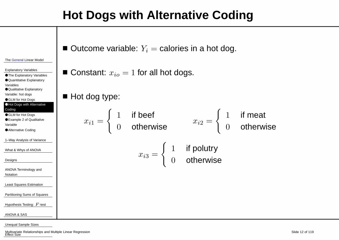
Hot Dogs with Alternative Coding
■ Outcome variable: Yi = calories in a hot dog.
■ Constant: xio = 1 for all hot dogs.
■ Hot dog type:
xi1 =
{
1 if beef0 otherwise
xi2 =
{
1 if meat0 otherwise
xi3 =
{
1 if polutry0 otherwise

The General Linear Model
Explanatory Variables
● The Explanatory Variables
● Quantitative Explanatory
Variables● Qualitative Explanatory
Variable: hot dogs
● GLM for Hot Dogs● Hot Dogs with Alternative
Coding
● GLM for Hot Dogs
● Example 2 of Qualitative
Variable
● Alternative Coding
1–Way Analysis of Variance
What & Whys of ANOVA
Designs
ANOVA Terminology and
Notation
Least Squares Estimation
Partitioning Sums of Squares
Hypothesis Testing: F -test
ANOVA & SAS
Unequal Sample Sizes
Effect SizeMultivariate Relationships and Multiple Linear Regression Slide 13 of 119
GLM for Hot Dogs
The General Linear Model,
Yi = βo + β1xi1 + β2xi2 + β3xi3 + ǫi
which when using our definitions of the variables is
caloriesi = βo + β1 + ǫi if beef
caloriesi = βo + β2 + ǫi if meat
caloriesi = βo + β3 + ǫi if poultry
This is the standard linear model used in ANOVA.

The General Linear Model
Explanatory Variables
● The Explanatory Variables
● Quantitative Explanatory
Variables● Qualitative Explanatory
Variable: hot dogs
● GLM for Hot Dogs● Hot Dogs with Alternative
Coding
● GLM for Hot Dogs
● Example 2 of Qualitative
Variable
● Alternative Coding
1–Way Analysis of Variance
What & Whys of ANOVA
Designs
ANOVA Terminology and
Notation
Least Squares Estimation
Partitioning Sums of Squares
Hypothesis Testing: F -test
ANOVA & SAS
Unequal Sample Sizes
Effect SizeMultivariate Relationships and Multiple Linear Regression Slide 14 of 119
Example 2 of Qualitative Variable
■ Let Yi = test score on exam.
■ A constant: xio = 1 for all individuals.
■ Teaching Method: web or text based.
xi1 =
{
1 if web based0 if text based
■ Simple linear model:
Yi = βoxio + β1xi1 + ǫi
Yi = βo + β1 + ǫi if web based
Yi = βo + ǫi if text based

The General Linear Model
Explanatory Variables
● The Explanatory Variables
● Quantitative Explanatory
Variables● Qualitative Explanatory
Variable: hot dogs
● GLM for Hot Dogs● Hot Dogs with Alternative
Coding
● GLM for Hot Dogs
● Example 2 of Qualitative
Variable
● Alternative Coding
1–Way Analysis of Variance
What & Whys of ANOVA
Designs
ANOVA Terminology and
Notation
Least Squares Estimation
Partitioning Sums of Squares
Hypothesis Testing: F -test
ANOVA & SAS
Unequal Sample Sizes
Effect SizeMultivariate Relationships and Multiple Linear Regression Slide 15 of 119
Alternative Coding
■ Let Yi = test score on exam.
■ A constant: xio = 1 for all individuals.
■ Teaching Method: web or text based.
xi1 =
{
1 if web based0 if text based
xi2 =
{
0 if web based1 if text based
■ The linear model,
Yi = βoxio + β1xi1 + β2xi2 + ǫi
Yi = βo + β1 + ǫi if web based
= βo + β2 + ǫi if text based

The General Linear Model
Explanatory Variables
1–Way Analysis of Variance
● 1–Way Analysis of Variance
What & Whys of ANOVA
Designs
ANOVA Terminology and
Notation
Least Squares Estimation
Partitioning Sums of Squares
Hypothesis Testing: F -test
ANOVA & SAS
Unequal Sample Sizes
Effect Size
Power
Violations of Assumptions
Multivariate Relationships and Multiple Linear Regression Slide 16 of 119
1–Way Analysis of VarianceOutline of Topics covered:
■ Introduction
◆ What it is and Why we need it.
◆ Experimental and Observational designs.
◆ Vocabulary, Terminology, Abbreviations, and Notation.
■ One–Factor ANOVA (fixed effects model).
◆ Least squares estimation.
◆ F–ratio and test.
◆ Summary.■ Effect of violations of assumptions.■ Power and Sensitively of ANOVA.■ More examples and other considerations.

The General Linear Model
Explanatory Variables
1–Way Analysis of Variance
What & Whys of ANOVA
● What & Whys of ANOVA
● Why ANOVA is Needed
● Familywise Error Rate
● Familywise Error Rate
● Familywise Error Rate
● Advantages of ANOVA
● Example of a 2-Way ANOVA
● Example of a 2-Way ANOVA
● Example of a 2-Way ANOVA
Designs
ANOVA Terminology and
Notation
Least Squares Estimation
Partitioning Sums of Squares
Hypothesis Testing: F -test
ANOVA & SAS
Unequal Sample Sizes
Effect Size
PowerMultivariate Relationships and Multiple Linear Regression Slide 17 of 119
What & Whys of ANOVA
Situation: One quantitative variable and one qualitative(discrete) variable:
■ Way to analyze the relationship between a quantitativevariable and a qualitative (discrete) variable.
■ Generalization of the two independent groups t-test.
■ The hypotheses tested in ANOVA is
Ho : µ1 = µ2 = . . . = µJ versus Ha : not all equal
where J equals the number of populations or groups.

The General Linear Model
Explanatory Variables
1–Way Analysis of Variance
What & Whys of ANOVA
● What & Whys of ANOVA
● Why ANOVA is Needed
● Familywise Error Rate
● Familywise Error Rate
● Familywise Error Rate
● Advantages of ANOVA
● Example of a 2-Way ANOVA
● Example of a 2-Way ANOVA
● Example of a 2-Way ANOVA
Designs
ANOVA Terminology and
Notation
Least Squares Estimation
Partitioning Sums of Squares
Hypothesis Testing: F -test
ANOVA & SAS
Unequal Sample Sizes
Effect Size
PowerMultivariate Relationships and Multiple Linear Regression Slide 18 of 119
Why ANOVA is Needed
■ Why not do possible two independent groups t-tests?
■ Consider Hot dog example, we would need 3 tests:
Ho1 : µbeef = µmeat, Ho2 : µbeef = µpolutry,
and Ho3 : µmeat = µpolutry
■ This strategy leads to J(J − 1)/2 t-tests,
Number of levels (J) Number of t–tests needed
4 4(4-1)/2=65 5(5-1)/2=106 6(6-1)/2 = 15...
...

The General Linear Model
Explanatory Variables
1–Way Analysis of Variance
What & Whys of ANOVA
● What & Whys of ANOVA
● Why ANOVA is Needed
● Familywise Error Rate
● Familywise Error Rate
● Familywise Error Rate
● Advantages of ANOVA
● Example of a 2-Way ANOVA
● Example of a 2-Way ANOVA
● Example of a 2-Way ANOVA
Designs
ANOVA Terminology and
Notation
Least Squares Estimation
Partitioning Sums of Squares
Hypothesis Testing: F -test
ANOVA & SAS
Unequal Sample Sizes
Effect Size
PowerMultivariate Relationships and Multiple Linear Regression Slide 19 of 119
Familywise Error Rate
■ Problem with all possible t-tests: If α = .05 for each test,then the probability of making a Type I error (on at least oneof the t-tests) is larger than .05.
■ The familywise error rate is the probability of Type I errors fora set of tests.
■ How big the problem is depends on
◆ The number of t-tests performed.
◆ Whether the t-tests are statistically independent.

The General Linear Model
Explanatory Variables
1–Way Analysis of Variance
What & Whys of ANOVA
● What & Whys of ANOVA
● Why ANOVA is Needed
● Familywise Error Rate
● Familywise Error Rate
● Familywise Error Rate
● Advantages of ANOVA
● Example of a 2-Way ANOVA
● Example of a 2-Way ANOVA
● Example of a 2-Way ANOVA
Designs
ANOVA Terminology and
Notation
Least Squares Estimation
Partitioning Sums of Squares
Hypothesis Testing: F -test
ANOVA & SAS
Unequal Sample Sizes
Effect Size
PowerMultivariate Relationships and Multiple Linear Regression Slide 20 of 119
Familywise Error Rate
If t-tests are independent and α = .05 for each one,
Then
P (at least one Type I error) = 1 − P (no type I errors)
= 1 − (1 − α)K
where K = the number of t-tests performed.
J = 3 −→ K = 3 −→ = 1 − (.95)3 = .14
J = 4 −→ K = 6 −→ = 1 − (.95)6 = .26
J = 5 −→ K = 10 −→ = 1 − (.95)10 = .40
J = 6 −→ K = 15 −→ = 1 − (.95)15 = .54

The General Linear Model
Explanatory Variables
1–Way Analysis of Variance
What & Whys of ANOVA
● What & Whys of ANOVA
● Why ANOVA is Needed
● Familywise Error Rate
● Familywise Error Rate
● Familywise Error Rate
● Advantages of ANOVA
● Example of a 2-Way ANOVA
● Example of a 2-Way ANOVA
● Example of a 2-Way ANOVA
Designs
ANOVA Terminology and
Notation
Least Squares Estimation
Partitioning Sums of Squares
Hypothesis Testing: F -test
ANOVA & SAS
Unequal Sample Sizes
Effect Size
PowerMultivariate Relationships and Multiple Linear Regression Slide 21 of 119
Familywise Error Rate■ Since the same data are used in more than one test, the
tests are dependent, which makes computing the actualfamilywise error rate very complex.
■ We do not know what the familywise error rate really equals.
■ The maximum familywise error rate is
P (at least one Type I error) ≤ Kα
which means that . . . The minimum and maximum familywiseerror rates for different numbers of t-tests are
K = 3, .14 ≤ P (at least one Type I error) ≤ 3(.05) = .15
K = 6, .26 ≤ P (at least one Type I error) ≤ 6(.05) = .30
K = 10, .40 ≤ P (at least one Type I error) ≤ 10(.05) = .50
K = 15, .54 ≤ P (at least one Type I error) ≤ 15(.05) = .75
Solution: Test the equality between all meanssimultaneously & set the familywise error rate.

The General Linear Model
Explanatory Variables
1–Way Analysis of Variance
What & Whys of ANOVA
● What & Whys of ANOVA
● Why ANOVA is Needed
● Familywise Error Rate
● Familywise Error Rate
● Familywise Error Rate
● Advantages of ANOVA
● Example of a 2-Way ANOVA
● Example of a 2-Way ANOVA
● Example of a 2-Way ANOVA
Designs
ANOVA Terminology and
Notation
Least Squares Estimation
Partitioning Sums of Squares
Hypothesis Testing: F -test
ANOVA & SAS
Unequal Sample Sizes
Effect Size
PowerMultivariate Relationships and Multiple Linear Regression Slide 22 of 119
Advantages of ANOVA
■ Control the familywise error rate when testing the equality ofmultiple populations’ means.
■ All of the data is used (in a single test), =⇒ better estimatesof population parameters.
■ Better estimates of population variance =⇒ ANOVA hasmore Power than all possible t-tests.
■ Multiple factors can be included.
◆ Effects due to different factors can be teased apart.
◆ Check for interaction effects.

The General Linear Model
Explanatory Variables
1–Way Analysis of Variance
What & Whys of ANOVA
● What & Whys of ANOVA
● Why ANOVA is Needed
● Familywise Error Rate
● Familywise Error Rate
● Familywise Error Rate
● Advantages of ANOVA
● Example of a 2-Way ANOVA
● Example of a 2-Way ANOVA
● Example of a 2-Way ANOVA
Designs
ANOVA Terminology and
Notation
Least Squares Estimation
Partitioning Sums of Squares
Hypothesis Testing: F -test
ANOVA & SAS
Unequal Sample Sizes
Effect Size
PowerMultivariate Relationships and Multiple Linear Regression Slide 23 of 119
Example of a 2-Way ANOVA
Example of multiple factor design: Wiley & Voss (1999)Constructing arguments from multiple sources: Tasks thatpromote understanding and not just memory for texts. Journal ofEducational Psychology, 91, 301–311.
■ Response/dependent variable = understanding as measuredby 10 item inference verification test (IVT), Yi = IVTi.
■ Factors:
◆ Format (text or web)
◆ Instructions participants received: write a Narrative (N),Summary (S), Explanation (E), Argument (A).

The General Linear Model
Explanatory Variables
1–Way Analysis of Variance
What & Whys of ANOVA
● What & Whys of ANOVA
● Why ANOVA is Needed
● Familywise Error Rate
● Familywise Error Rate
● Familywise Error Rate
● Advantages of ANOVA
● Example of a 2-Way ANOVA
● Example of a 2-Way ANOVA
● Example of a 2-Way ANOVA
Designs
ANOVA Terminology and
Notation
Least Squares Estimation
Partitioning Sums of Squares
Hypothesis Testing: F -test
ANOVA & SAS
Unequal Sample Sizes
Effect Size
PowerMultivariate Relationships and Multiple Linear Regression Slide 24 of 119
Example of a 2-Way ANOVA
Summary statistics: Y and s2, where ncell = 8.
InstructionsFormat N S E A Total
Text 71.25 72.5 68.75 73.75 71.56126.79 164.29 69.64 141.07
Web 76.25 73.75 72.5 90.0 78.1255.36 255.36 107.14 114.29
Totals 73.75 73.13 70.63 81.88 74.84
From Meyers & Well (2003). Research Design and Statistical Analysis.

The General Linear Model
Explanatory Variables
1–Way Analysis of Variance
What & Whys of ANOVA
● What & Whys of ANOVA
● Why ANOVA is Needed
● Familywise Error Rate
● Familywise Error Rate
● Familywise Error Rate
● Advantages of ANOVA
● Example of a 2-Way ANOVA
● Example of a 2-Way ANOVA
● Example of a 2-Way ANOVA
Designs
ANOVA Terminology and
Notation
Least Squares Estimation
Partitioning Sums of Squares
Hypothesis Testing: F -test
ANOVA & SAS
Unequal Sample Sizes
Effect Size
PowerMultivariate Relationships and Multiple Linear Regression Slide 25 of 119
Example of a 2-Way ANOVA
Possible null hypotheses that can be tested:
■ Main effects:◆ Effect of Instruction:
Ho1 : µN = µS = µE = µA
◆ Effect of Format:
Ho2 : µtext = µweb
■ Interaction of instruction and format: Ho3 :
µN,text = µN,web = µE,text = µE,web = µS,text = µS,web = µA,text = µA,web
The General Linear Model
Explanatory Variables
1–Way Analysis of Variance
What & Whys of ANOVA
Designs
● Designs
● Experimental Designs
● An Example of a C.R.
Experimental Design
● Random Assignment in C.R.
Designs
● Observational Studies● Observational versus
Experimental
● Different Designs
ANOVA Terminology and
Notation
Least Squares Estimation
Partitioning Sums of Squares
Hypothesis Testing: F -test
ANOVA & SAS
Unequal Sample Sizes
Effect Size
PowerMultivariate Relationships and Multiple Linear Regression Slide 26 of 119
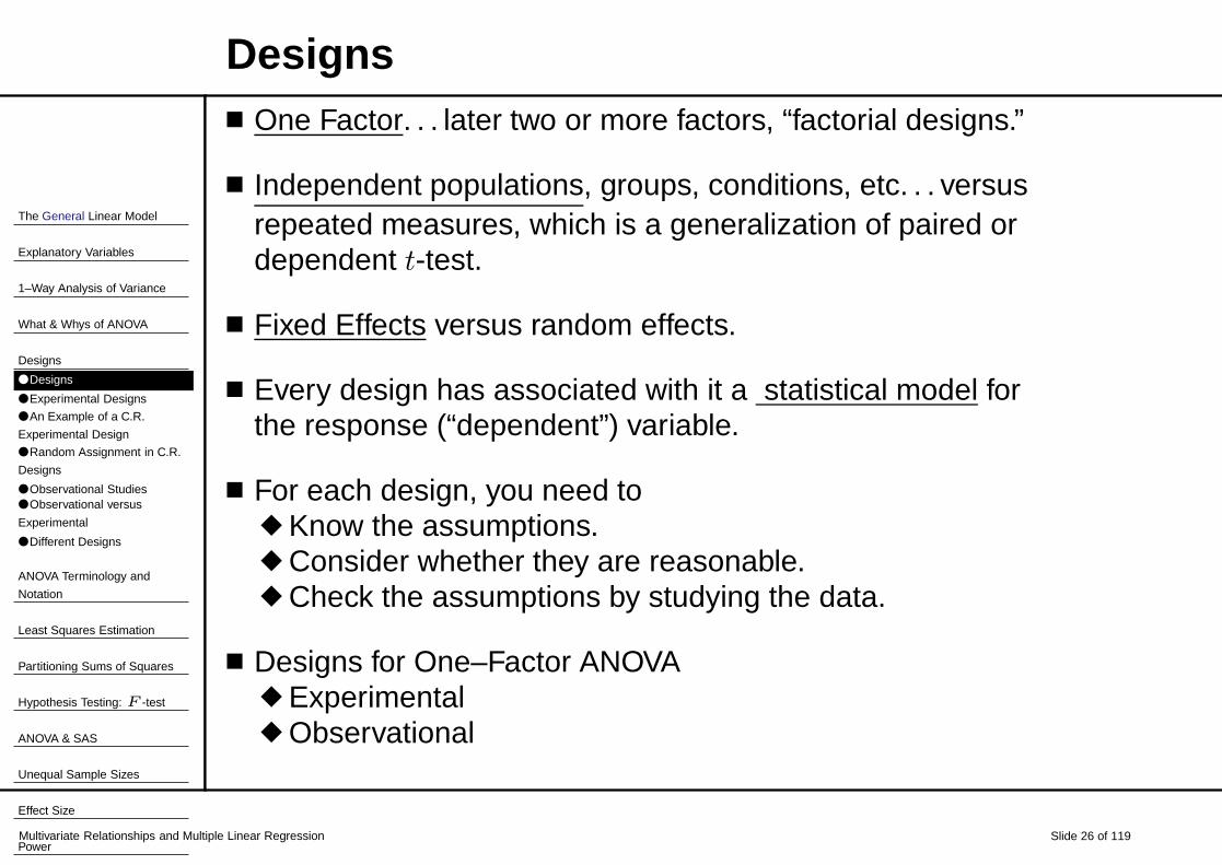
Designs■ One Factor. . . later two or more factors, “factorial designs.”
■ Independent populations, groups, conditions, etc. . . versusrepeated measures, which is a generalization of paired ordependent t-test.
■ Fixed Effects versus random effects.
■ Every design has associated with it a statistical model forthe response (“dependent”) variable.
■ For each design, you need to◆ Know the assumptions.◆ Consider whether they are reasonable.◆ Check the assumptions by studying the data.
■ Designs for One–Factor ANOVA◆ Experimental◆ Observational

The General Linear Model
Explanatory Variables
1–Way Analysis of Variance
What & Whys of ANOVA
Designs
● Designs
● Experimental Designs
● An Example of a C.R.
Experimental Design
● Random Assignment in C.R.
Designs
● Observational Studies● Observational versus
Experimental
● Different Designs
ANOVA Terminology and
Notation
Least Squares Estimation
Partitioning Sums of Squares
Hypothesis Testing: F -test
ANOVA & SAS
Unequal Sample Sizes
Effect Size
PowerMultivariate Relationships and Multiple Linear Regression Slide 27 of 119
Experimental Designs
Completely Randomized Experimental Design
■ Subjects are randomly assigned to one and only onecondition (Note: “Subject” does not have to be a person. Itcould be a school, donut, etc.)
■ The different conditions are the levels of the independentvariable or factor, which are discrete.
■ The dependent variable is numerical measure of which wewant to know whether the independent variable has an effecton.

The General Linear Model
Explanatory Variables
1–Way Analysis of Variance
What & Whys of ANOVA
Designs
● Designs
● Experimental Designs
● An Example of a C.R.
Experimental Design
● Random Assignment in C.R.
Designs
● Observational Studies● Observational versus
Experimental
● Different Designs
ANOVA Terminology and
Notation
Least Squares Estimation
Partitioning Sums of Squares
Hypothesis Testing: F -test
ANOVA & SAS
Unequal Sample Sizes
Effect Size
PowerMultivariate Relationships and Multiple Linear Regression Slide 28 of 119
An Example of a C.R. Experimental Design
Wiley & Voss (1999)
■ Students are random assigned to received one type ofInstruction. Type of instruction is independent variable and ithas four levels.
■ The amount learned (IVT measure) is the dependentvariables.
Goal: Make causal inferences about the effects of independentvariables on the dependent variable.

The General Linear Model
Explanatory Variables
1–Way Analysis of Variance
What & Whys of ANOVA
Designs
● Designs
● Experimental Designs
● An Example of a C.R.
Experimental Design
● Random Assignment in C.R.
Designs
● Observational Studies● Observational versus
Experimental
● Different Designs
ANOVA Terminology and
Notation
Least Squares Estimation
Partitioning Sums of Squares
Hypothesis Testing: F -test
ANOVA & SAS
Unequal Sample Sizes
Effect Size
PowerMultivariate Relationships and Multiple Linear Regression Slide 29 of 119
Random Assignment in C.R. Designs
■ The random assignment to conditions is required so that
◆ The value of the dependent variable is not related to thecondition to which a person is assigned to.
◆ Assignment to conditions (treatments) is not confoundedwith treatment.
◆ Any differences between groups (conditions) with respectto subjects’ assigned to them are unsystematic.
■ Question answered by ANOVA with a completely randomizedexperimental design:
◆ Are differences on average (mean) responses ormeasures between conditions due to chance error or arethe differences large enough to indicate that there are realdifferences in the population?
◆ Are treatment effects different?

The General Linear Model
Explanatory Variables
1–Way Analysis of Variance
What & Whys of ANOVA
Designs
● Designs
● Experimental Designs
● An Example of a C.R.
Experimental Design
● Random Assignment in C.R.
Designs
● Observational Studies● Observational versus
Experimental
● Different Designs
ANOVA Terminology and
Notation
Least Squares Estimation
Partitioning Sums of Squares
Hypothesis Testing: F -test
ANOVA & SAS
Unequal Sample Sizes
Effect Size
PowerMultivariate Relationships and Multiple Linear Regression Slide 30 of 119
Observational Studies
■ Take Random samples from different populations.
■ Random sampling is required to get samples that arerepresentative of the populations that are of interest.
■ We do not want samples that differ from the population insome systematic way.
■ If samples differ systematically, then we have a confoundbetween conditions and selection.
An observational version of Wiley & Voss study:
■ Take a random sample of students who were required to dodifferent types of writing assignments and have them takethe IVT.
■ Type of writing assignment is the explanatory variable.■ Obtain measure of learning (e.g., IVT).■ IVTis the Response variable.

The General Linear Model
Explanatory Variables
1–Way Analysis of Variance
What & Whys of ANOVA
Designs
● Designs
● Experimental Designs
● An Example of a C.R.
Experimental Design
● Random Assignment in C.R.
Designs
● Observational Studies● Observational versus
Experimental
● Different Designs
ANOVA Terminology and
Notation
Least Squares Estimation
Partitioning Sums of Squares
Hypothesis Testing: F -test
ANOVA & SAS
Unequal Sample Sizes
Effect Size
PowerMultivariate Relationships and Multiple Linear Regression Slide 31 of 119
Observational versus Experimental
■ In observational studies, the factor is called an explanatoryvariable rather than an independent variable.
■ In observational studies, response or criterion variablesinstead of dependent variables.
■ Why the difference in terminology?
◆ In observational studies, Cannot make causal inferences.
◆ In observational studies, Can make inferences aboutwhether differences exist.

The General Linear Model
Explanatory Variables
1–Way Analysis of Variance
What & Whys of ANOVA
Designs
● Designs
● Experimental Designs
● An Example of a C.R.
Experimental Design
● Random Assignment in C.R.
Designs
● Observational Studies● Observational versus
Experimental
● Different Designs
ANOVA Terminology and
Notation
Least Squares Estimation
Partitioning Sums of Squares
Hypothesis Testing: F -test
ANOVA & SAS
Unequal Sample Sizes
Effect Size
PowerMultivariate Relationships and Multiple Linear Regression Slide 32 of 119
Different Designs
■ In observational studies, should not conclude that
◆ “differences are caused by ”
◆ “the effect of” factor levels on . . . ”
■ Differences between experimental and observationaldesigns −→ differences in
◆ Terminology
◆ Conclusions
■ But the statistics and mathematical procedures are thesame.

The General Linear Model
Explanatory Variables
1–Way Analysis of Variance
What & Whys of ANOVA
Designs
ANOVA Terminology and
Notation● ANOVA Terminology and
Notation
● Design/Model Specific
● Notation
● More Notation● Working Example of 1-factor
ANOVA
● The Wiley & Voss Data
● The Wiley & Voss Data
● Working Example for 1-Factor
ANOVA
Least Squares Estimation
Partitioning Sums of Squares
Hypothesis Testing: F -test
ANOVA & SAS
Unequal Sample Sizes
Effect Size
Power
Multivariate Relationships and Multiple Linear Regression Slide 33 of 119
ANOVA Terminology and Notation
General:
■ ANOVA ≡ ANalysis Of VAriance■ Familywise error rate ≡ Prob(Type I error in the whole set of
tests)■ Factor ≡ Explanatory or Independent variable. It’s discrete
(nominal or ordinal) and observable.■ Levels of a factor ≡ Categories of the factor■ Dependent or Response variable≡ What’s being measured
(“construct of interest”); whether there’s a difference.■ Effect ≡ variability due to difference sources (e.g., error,
treatment or group, etc)■ Replicates ≡ usually subjects or individuals■ Source (of variation) ≡ error and treatment or group (for
now)■ Treatment effects (systematic) ≡ systematic variability■ Experimental Error (unsystematic) ≡ unsystematic variability

The General Linear Model
Explanatory Variables
1–Way Analysis of Variance
What & Whys of ANOVA
Designs
ANOVA Terminology and
Notation● ANOVA Terminology and
Notation
● Design/Model Specific
● Notation
● More Notation● Working Example of 1-factor
ANOVA
● The Wiley & Voss Data
● The Wiley & Voss Data
● Working Example for 1-Factor
ANOVA
Least Squares Estimation
Partitioning Sums of Squares
Hypothesis Testing: F -test
ANOVA & SAS
Unequal Sample Sizes
Effect Size
Power
Multivariate Relationships and Multiple Linear Regression Slide 34 of 119
Design/Model Specific
■ Completely Randomized experimental Design — or CRD
■ Observational design/study
■ Factorial design — more than one factor
■ Balanced design — n1 = n2 = . . . = nJ = n
■ Fixed effects —
■ Random effects
■ Repeated measures
■ Crossed Factors
■ Nested Factors
■ Blocking Factor(s)

The General Linear Model
Explanatory Variables
1–Way Analysis of Variance
What & Whys of ANOVA
Designs
ANOVA Terminology and
Notation● ANOVA Terminology and
Notation
● Design/Model Specific
● Notation
● More Notation● Working Example of 1-factor
ANOVA
● The Wiley & Voss Data
● The Wiley & Voss Data
● Working Example for 1-Factor
ANOVA
Least Squares Estimation
Partitioning Sums of Squares
Hypothesis Testing: F -test
ANOVA & SAS
Unequal Sample Sizes
Effect Size
Power
Multivariate Relationships and Multiple Linear Regression Slide 35 of 119
Notation(some conventions specific to 1–Factor ANOVA)
■ SS (sums of squares).
■ MS (means squared errors).
■ Upper case Roman letters refer to factors (e.g., A, B, . . . ).
■ S to refer to subject.
■ S|A subject within factor A.
■ y refers to observations on the dependent or responsevariable.
■ i index subjects (experimental unit, replicate, etc.)
■ j index levels of a factor
■ So Yij is the observation on subject i at level j of the factor.
■ J number of levels of a factor

The General Linear Model
Explanatory Variables
1–Way Analysis of Variance
What & Whys of ANOVA
Designs
ANOVA Terminology and
Notation● ANOVA Terminology and
Notation
● Design/Model Specific
● Notation
● More Notation● Working Example of 1-factor
ANOVA
● The Wiley & Voss Data
● The Wiley & Voss Data
● Working Example for 1-Factor
ANOVA
Least Squares Estimation
Partitioning Sums of Squares
Hypothesis Testing: F -test
ANOVA & SAS
Unequal Sample Sizes
Effect Size
Power
Multivariate Relationships and Multiple Linear Regression Slide 36 of 119
More Notation■ nj number of subjects assigned to (observed at) level j of
the factor.
■ N =∑J
j=1 nj = total number of subjects.
■ n+ = N (sometimes)
■ Yj = (1/nj)∑nj
j=1 Yij = sample mean for level j.
■ Y = (1/N)∑J
j=1
∑nj
i=1 Yij =
grand (sample) mean.
■ µ grand mean in population.
■ σ2ǫ = experimental (unsystematic, within groups) error.
■ µj = population mean for level j of the factor.
■ αj = population treatment effect for level j of factor.
■ ǫij = residual or error for subject i for level j.

The General Linear Model
Explanatory Variables
1–Way Analysis of Variance
What & Whys of ANOVA
Designs
ANOVA Terminology and
Notation● ANOVA Terminology and
Notation
● Design/Model Specific
● Notation
● More Notation● Working Example of 1-factor
ANOVA
● The Wiley & Voss Data
● The Wiley & Voss Data
● Working Example for 1-Factor
ANOVA
Least Squares Estimation
Partitioning Sums of Squares
Hypothesis Testing: F -test
ANOVA & SAS
Unequal Sample Sizes
Effect Size
Power
Multivariate Relationships and Multiple Linear Regression Slide 37 of 119
Working Example of 1-factor ANOVA
Consider the Wiley & Voss data:Instructions
Statistic N S E A Total
means 73.75 73.13 70.63 81.88 74.84sj 13.60 14.01 9.29 13.77 13.21s2
j 185.00 196.25 86.25 189.58 174.58nj 16 16 16 16 64
Define IVT = Yij for student/particpant i in jth level.

The General Linear Model
Explanatory Variables
1–Way Analysis of Variance
What & Whys of ANOVA
Designs
ANOVA Terminology and
Notation● ANOVA Terminology and
Notation
● Design/Model Specific
● Notation
● More Notation● Working Example of 1-factor
ANOVA
● The Wiley & Voss Data
● The Wiley & Voss Data
● Working Example for 1-Factor
ANOVA
Least Squares Estimation
Partitioning Sums of Squares
Hypothesis Testing: F -test
ANOVA & SAS
Unequal Sample Sizes
Effect Size
Power
Multivariate Relationships and Multiple Linear Regression Slide 38 of 119
The Wiley & Voss Data

The General Linear Model
Explanatory Variables
1–Way Analysis of Variance
What & Whys of ANOVA
Designs
ANOVA Terminology and
Notation● ANOVA Terminology and
Notation
● Design/Model Specific
● Notation
● More Notation● Working Example of 1-factor
ANOVA
● The Wiley & Voss Data
● The Wiley & Voss Data
● Working Example for 1-Factor
ANOVA
Least Squares Estimation
Partitioning Sums of Squares
Hypothesis Testing: F -test
ANOVA & SAS
Unequal Sample Sizes
Effect Size
Power
Multivariate Relationships and Multiple Linear Regression Slide 39 of 119
The Wiley & Voss Data

The General Linear Model
Explanatory Variables
1–Way Analysis of Variance
What & Whys of ANOVA
Designs
ANOVA Terminology and
Notation● ANOVA Terminology and
Notation
● Design/Model Specific
● Notation
● More Notation● Working Example of 1-factor
ANOVA
● The Wiley & Voss Data
● The Wiley & Voss Data
● Working Example for 1-Factor
ANOVA
Least Squares Estimation
Partitioning Sums of Squares
Hypothesis Testing: F -test
ANOVA & SAS
Unequal Sample Sizes
Effect Size
Power
Multivariate Relationships and Multiple Linear Regression Slide 40 of 119
Working Example for 1-Factor ANOVA■ Define Xio = 1 and
Xi1 =
{
1 if Narrative0 otherwise
Xi2 =
{
1 if Summary0 otherwise
Xi3 =
{
1 if Explanation0 otherwise
Xi4 =
{
1 if Argument0 otherwise
■ Yi = βoxio + β1xi1 + β2xi2 + β3xi3 + β4xi4 + ǫi
■ By level of instruction factor:
Yi =
βo + β1 + ǫi if Narrativeβo + +β2 + ǫi if Summaryβo + +β3 + ǫi if Explainβo + +β4 + ǫi if Argument
■ What do the weights (i.e., β’s) equal?

The General Linear Model
Explanatory Variables
1–Way Analysis of Variance
What & Whys of ANOVA
Designs
ANOVA Terminology and
Notation
Least Squares Estimation
● Least Squares Estimation
● Least Squares Estimation
● Least Squares Estimation
● Least Squares Estimation
● Least Squares Estimation
● Example: Least Squares
Estimation● Population 1 Factor ANOVA
Model
● Picture of ANOVA
● Picture of ANOVA
● Picture of ANOVA
Partitioning Sums of Squares
Hypothesis Testing: F -test
ANOVA & SAS
Unequal Sample Sizes
Effect SizeMultivariate Relationships and Multiple Linear Regression Slide 41 of 119
Least Squares Estimation
■ ǫi = Yi − (βo + β1xi1 + β2xi2 + β3xi3 + β4xi4).■ Want β’s that minimize the error variance,
1
N
N∑
i=1
(ǫi − ǫi)2
■ Two restrictions:∑N
i=1 ǫi = 0 and∑J
j=1 βj = 0.
■ The “loss function” is then
sumNi=1(ǫi − ǫi)
2 =N∑
i=1
(Yi − (βo + β1xi1 + β2xi2 + β3xi3 + β4xi4))2
=N∑
i=1
(Yi − guess)2

The General Linear Model
Explanatory Variables
1–Way Analysis of Variance
What & Whys of ANOVA
Designs
ANOVA Terminology and
Notation
Least Squares Estimation
● Least Squares Estimation
● Least Squares Estimation
● Least Squares Estimation
● Least Squares Estimation
● Least Squares Estimation
● Example: Least Squares
Estimation● Population 1 Factor ANOVA
Model
● Picture of ANOVA
● Picture of ANOVA
● Picture of ANOVA
Partitioning Sums of Squares
Hypothesis Testing: F -test
ANOVA & SAS
Unequal Sample Sizes
Effect SizeMultivariate Relationships and Multiple Linear Regression Slide 42 of 119
Least Squares Estimation■ Let Yij = observation for individual i from group j.■ What minimizes this?
nj∑
i=1
(yij − guessj)2
■ The group mean, yj =∑nj
i=1 yij/nj
■ Re-write the loss function as
J∑
j=1
nj∑
i=1
(Yij − guessj)2 =
n1∑
i=1
(yi1 − ?1)2 +
n2∑
i=1
(yi2 − ?2)2
n3∑
i=3
(yi3 − ?3)2 +
n4∑
i=1
(yi4 − ?4)2
■ If we minimize each one of these, we minimize their sum.■ Let’s consider the first one (i.e., for Narrative). . .

The General Linear Model
Explanatory Variables
1–Way Analysis of Variance
What & Whys of ANOVA
Designs
ANOVA Terminology and
Notation
Least Squares Estimation
● Least Squares Estimation
● Least Squares Estimation
● Least Squares Estimation
● Least Squares Estimation
● Least Squares Estimation
● Example: Least Squares
Estimation● Population 1 Factor ANOVA
Model
● Picture of ANOVA
● Picture of ANOVA
● Picture of ANOVA
Partitioning Sums of Squares
Hypothesis Testing: F -test
ANOVA & SAS
Unequal Sample Sizes
Effect SizeMultivariate Relationships and Multiple Linear Regression Slide 43 of 119
Least Squares Estimation
∑n1
i=1(yi1 − ?1)2
■ Setting ?1 = y1 = ynarrative minimizes this.
■ Filling in our linear model for Narrative:
n1∑
i=1
(yi1 − y1)2 =
n1∑
i=1
(yi1 − (βo + β1))2
■ So, y1 = ynarrative = βo + β1
■ For all of them
y1 = ynarrative = βo + β1, y2 = ysummary = βo + β2
y3 = yexplanation = βo + β3, y4 = yargument = βo + β4

The General Linear Model
Explanatory Variables
1–Way Analysis of Variance
What & Whys of ANOVA
Designs
ANOVA Terminology and
Notation
Least Squares Estimation
● Least Squares Estimation
● Least Squares Estimation
● Least Squares Estimation
● Least Squares Estimation
● Least Squares Estimation
● Example: Least Squares
Estimation● Population 1 Factor ANOVA
Model
● Picture of ANOVA
● Picture of ANOVA
● Picture of ANOVA
Partitioning Sums of Squares
Hypothesis Testing: F -test
ANOVA & SAS
Unequal Sample Sizes
Effect SizeMultivariate Relationships and Multiple Linear Regression Slide 44 of 119
Least Squares Estimation
y1 = ynarrative = βo + β1, y2 = ysummary = βo + β2
y3 = yexplanation = βo + β3, y4 = yargument = βo + β4
■ Solution for βo:
βo = y =1
∑Nj=1 nj
N∑
j=1
nj∑
i=1
yij = grand mean
■ Solution for βj = (group mean)j − (grand mean):
β1 = y1 − y, β2 = y2 − y
β3 = y3 − y, β4 = y4 − y

The General Linear Model
Explanatory Variables
1–Way Analysis of Variance
What & Whys of ANOVA
Designs
ANOVA Terminology and
Notation
Least Squares Estimation
● Least Squares Estimation
● Least Squares Estimation
● Least Squares Estimation
● Least Squares Estimation
● Least Squares Estimation
● Example: Least Squares
Estimation● Population 1 Factor ANOVA
Model
● Picture of ANOVA
● Picture of ANOVA
● Picture of ANOVA
Partitioning Sums of Squares
Hypothesis Testing: F -test
ANOVA & SAS
Unequal Sample Sizes
Effect SizeMultivariate Relationships and Multiple Linear Regression Slide 45 of 119
Least Squares Estimation
■ More conventional notation is that βj = αj , the effect of levelj of the factor.
■ So our estimated model is
Yij = Y + αj
= Y + (Yj − Y )
= Yj

The General Linear Model
Explanatory Variables
1–Way Analysis of Variance
What & Whys of ANOVA
Designs
ANOVA Terminology and
Notation
Least Squares Estimation
● Least Squares Estimation
● Least Squares Estimation
● Least Squares Estimation
● Least Squares Estimation
● Least Squares Estimation
● Example: Least Squares
Estimation● Population 1 Factor ANOVA
Model
● Picture of ANOVA
● Picture of ANOVA
● Picture of ANOVA
Partitioning Sums of Squares
Hypothesis Testing: F -test
ANOVA & SAS
Unequal Sample Sizes
Effect SizeMultivariate Relationships and Multiple Linear Regression Slide 46 of 119
Example: Least Squares EstimationFor the Wiley & Voss data:
InstructionsStatistic N S E A Total
means 73.75 73.13 70.63 81.88 74.84sj 13.60 14.01 9.29 13.77 13.21nj 16 16 16 16 64
yi1 = yi,narrative = 74.84 + (73.75 − 74.84) = 74.84 − 1.09
yi2 = yi,summary = 74.84 + (73.13 − 74.84) = 74.84 − 1.71
yi3 = yi,explanation = 74.84 + (70.63 − 74.84) = 74.84 − 4.21
yi4 = yi,argument = 74.84 + (81.88 − 74.84) = 74.84 + 7.04

The General Linear Model
Explanatory Variables
1–Way Analysis of Variance
What & Whys of ANOVA
Designs
ANOVA Terminology and
Notation
Least Squares Estimation
● Least Squares Estimation
● Least Squares Estimation
● Least Squares Estimation
● Least Squares Estimation
● Least Squares Estimation
● Example: Least Squares
Estimation● Population 1 Factor ANOVA
Model
● Picture of ANOVA
● Picture of ANOVA
● Picture of ANOVA
Partitioning Sums of Squares
Hypothesis Testing: F -test
ANOVA & SAS
Unequal Sample Sizes
Effect SizeMultivariate Relationships and Multiple Linear Regression Slide 47 of 119
Population 1 Factor ANOVA Model
■ The 1-factor ANOVA model:
Yij = µ + αj + ǫij
■ µ = grand mean over all populations.
■ αj = µj − µ
■ ǫ ∼ N (0, σ2ǫ ) i.i.d.
■ Estimation of the model (given data):
Yij = µ + αj + ǫij
= Y + (Yj − Y ) + (Yij − Yj)

The General Linear Model
Explanatory Variables
1–Way Analysis of Variance
What & Whys of ANOVA
Designs
ANOVA Terminology and
Notation
Least Squares Estimation
● Least Squares Estimation
● Least Squares Estimation
● Least Squares Estimation
● Least Squares Estimation
● Least Squares Estimation
● Example: Least Squares
Estimation● Population 1 Factor ANOVA
Model
● Picture of ANOVA
● Picture of ANOVA
● Picture of ANOVA
Partitioning Sums of Squares
Hypothesis Testing: F -test
ANOVA & SAS
Unequal Sample Sizes
Effect SizeMultivariate Relationships and Multiple Linear Regression Slide 48 of 119
Picture of ANOVA

The General Linear Model
Explanatory Variables
1–Way Analysis of Variance
What & Whys of ANOVA
Designs
ANOVA Terminology and
Notation
Least Squares Estimation
● Least Squares Estimation
● Least Squares Estimation
● Least Squares Estimation
● Least Squares Estimation
● Least Squares Estimation
● Example: Least Squares
Estimation● Population 1 Factor ANOVA
Model
● Picture of ANOVA
● Picture of ANOVA
● Picture of ANOVA
Partitioning Sums of Squares
Hypothesis Testing: F -test
ANOVA & SAS
Unequal Sample Sizes
Effect SizeMultivariate Relationships and Multiple Linear Regression Slide 49 of 119
Picture of ANOVA

The General Linear Model
Explanatory Variables
1–Way Analysis of Variance
What & Whys of ANOVA
Designs
ANOVA Terminology and
Notation
Least Squares Estimation
● Least Squares Estimation
● Least Squares Estimation
● Least Squares Estimation
● Least Squares Estimation
● Least Squares Estimation
● Example: Least Squares
Estimation● Population 1 Factor ANOVA
Model
● Picture of ANOVA
● Picture of ANOVA
● Picture of ANOVA
Partitioning Sums of Squares
Hypothesis Testing: F -test
ANOVA & SAS
Unequal Sample Sizes
Effect SizeMultivariate Relationships and Multiple Linear Regression Slide 50 of 119
Picture of ANOVA

The General Linear Model
Explanatory Variables
1–Way Analysis of Variance
What & Whys of ANOVA
Designs
ANOVA Terminology and
Notation
Least Squares Estimation
Partitioning Sums of Squares
● Partitioning Sums of Squares
● Partitioning Sums of Squares
● Work Through the Algebra● Work Through the Algebra
(continued)
● The ANOVA Decomposition
● Example: Sums of Squares
Decomposition
● Example: Sums of Squares
Decomposition
● Example: Sums of Squares
Decomposition.
● Example: Sums of Squares
Decomposition
● Brief Digression/Note
● Decomposition of Variance
● Proportion of Variance
● Proportion of Variance
● Multiple R Squared
Hypothesis Testing: F -test
Multivariate Relationships and Multiple Linear Regression Slide 51 of 119
Partitioning Sums of Squares■ How do we test the null hypothesis?
■ Study the variance.
■ According to our model
Yij = µ + αj + ǫij
= Y + (Yj − Y ) + (Yij − Yj)
or
(Yij − Y ) = (Yj − Y ) + (Yij − Yj)
deviation of
score from
overall mean
=
deviation of
group mean
from overall
+
deviation of
score from
group mean

The General Linear Model
Explanatory Variables
1–Way Analysis of Variance
What & Whys of ANOVA
Designs
ANOVA Terminology and
Notation
Least Squares Estimation
Partitioning Sums of Squares
● Partitioning Sums of Squares
● Partitioning Sums of Squares
● Work Through the Algebra● Work Through the Algebra
(continued)
● The ANOVA Decomposition
● Example: Sums of Squares
Decomposition
● Example: Sums of Squares
Decomposition
● Example: Sums of Squares
Decomposition.
● Example: Sums of Squares
Decomposition
● Brief Digression/Note
● Decomposition of Variance
● Proportion of Variance
● Proportion of Variance
● Multiple R Squared
Hypothesis Testing: F -test
Multivariate Relationships and Multiple Linear Regression Slide 52 of 119
Partitioning Sums of Squares
(Yij − Y ) = (Yj − Y ) + (Yij − Yj)■ Square both sides,
(Yij − Y )2 =[
(Yj − Y ) + (Yij − Yj)]2
■ Sum over all groups and individuals with groups,
J∑
j=1
nj∑
i=1
(Yij − Y )2 =
J∑
j=1
nj∑
i=1
[(Yj − Y ) + (Yij − Yj)]2

The General Linear Model
Explanatory Variables
1–Way Analysis of Variance
What & Whys of ANOVA
Designs
ANOVA Terminology and
Notation
Least Squares Estimation
Partitioning Sums of Squares
● Partitioning Sums of Squares
● Partitioning Sums of Squares
● Work Through the Algebra● Work Through the Algebra
(continued)
● The ANOVA Decomposition
● Example: Sums of Squares
Decomposition
● Example: Sums of Squares
Decomposition
● Example: Sums of Squares
Decomposition.
● Example: Sums of Squares
Decomposition
● Brief Digression/Note
● Decomposition of Variance
● Proportion of Variance
● Proportion of Variance
● Multiple R Squared
Hypothesis Testing: F -test
Multivariate Relationships and Multiple Linear Regression Slide 53 of 119
Work Through the Algebra
J∑
j=1
nj∑
i=1
(Yij − Y )2 =J∑
j=1
nj∑
i=1
[
(Yj − Y ) + (Yij − Yj)]2
=J∑
j=1
nj∑
i=1
[
(Yj − Y )2 + (Yij − Yj)2
+2(Yj − Y )(Yij − Yj)]
=J∑
j=1
nj∑
i=1
(Yj − Y )2 +J∑
j=1
nj∑
i=1
(Yij − Yj)2
+J∑
j=1
nj∑
i=1
2(Yj − Y )(Yij − Yj)

The General Linear Model
Explanatory Variables
1–Way Analysis of Variance
What & Whys of ANOVA
Designs
ANOVA Terminology and
Notation
Least Squares Estimation
Partitioning Sums of Squares
● Partitioning Sums of Squares
● Partitioning Sums of Squares
● Work Through the Algebra● Work Through the Algebra
(continued)
● The ANOVA Decomposition
● Example: Sums of Squares
Decomposition
● Example: Sums of Squares
Decomposition
● Example: Sums of Squares
Decomposition.
● Example: Sums of Squares
Decomposition
● Brief Digression/Note
● Decomposition of Variance
● Proportion of Variance
● Proportion of Variance
● Multiple R Squared
Hypothesis Testing: F -test
Multivariate Relationships and Multiple Linear Regression Slide 54 of 119
Work Through the Algebra (continued)
J∑
j=1
nj∑
i=1
(Yij − Y )2 =J∑
j=1
nj∑
i=1
(Yj − Y )2 +J∑
j=1
nj∑
i=1
(Yij − Yj)2
+J∑
j=1
nj∑
i=1
2(Yj − Y )(Yij − Yj)
=
J∑
j=1
nj(Yj − Y )2+
J∑
j=1
nj∑
i=1
(Yij − Yj)2
+2J∑
j=1
(Yj − Y )
nj∑
i=1
(Yij − Yj)
=J∑
j=1
nj(Yj − Y )2 +J∑
j=1
nj∑
i=1
(Yij − Yj)2

The General Linear Model
Explanatory Variables
1–Way Analysis of Variance
What & Whys of ANOVA
Designs
ANOVA Terminology and
Notation
Least Squares Estimation
Partitioning Sums of Squares
● Partitioning Sums of Squares
● Partitioning Sums of Squares
● Work Through the Algebra● Work Through the Algebra
(continued)
● The ANOVA Decomposition
● Example: Sums of Squares
Decomposition
● Example: Sums of Squares
Decomposition
● Example: Sums of Squares
Decomposition.
● Example: Sums of Squares
Decomposition
● Brief Digression/Note
● Decomposition of Variance
● Proportion of Variance
● Proportion of Variance
● Multiple R Squared
Hypothesis Testing: F -test
Multivariate Relationships and Multiple Linear Regression Slide 55 of 119
The ANOVA Decomposition
J∑
j=1
nj∑
i=1
(Yij − Y )2 =J∑
j=1
nj(Yj − Y )2 +J∑
j=1
nj∑
i=1
(Yij − Yj)2
SStotal = SSbetween + SSwithtin
SStotal=SSmodel + SSerror
■ SStotal is “corrected for mean”
■ SSwithin also gets called
◆ SSerror◆ SSresidual◆ SSS|A, “subjects within factor A”

The General Linear Model
Explanatory Variables
1–Way Analysis of Variance
What & Whys of ANOVA
Designs
ANOVA Terminology and
Notation
Least Squares Estimation
Partitioning Sums of Squares
● Partitioning Sums of Squares
● Partitioning Sums of Squares
● Work Through the Algebra● Work Through the Algebra
(continued)
● The ANOVA Decomposition
● Example: Sums of Squares
Decomposition
● Example: Sums of Squares
Decomposition
● Example: Sums of Squares
Decomposition.
● Example: Sums of Squares
Decomposition
● Brief Digression/Note
● Decomposition of Variance
● Proportion of Variance
● Proportion of Variance
● Multiple R Squared
Hypothesis Testing: F -test
Multivariate Relationships and Multiple Linear Regression Slide 56 of 119
Example: Sums of Squares Decomposition
Wiley & Voss Data(note: summary statistics on pages 40 and 51)
SStotal =J∑
j=1
nj∑
i=1
(Yij − Y )2
=4∑
j=1
16∑
i=1
(Yij − 74.84)2
= (N − 1)s2
= (64 − 1)174.578
= 10, 998.414

The General Linear Model
Explanatory Variables
1–Way Analysis of Variance
What & Whys of ANOVA
Designs
ANOVA Terminology and
Notation
Least Squares Estimation
Partitioning Sums of Squares
● Partitioning Sums of Squares
● Partitioning Sums of Squares
● Work Through the Algebra● Work Through the Algebra
(continued)
● The ANOVA Decomposition
● Example: Sums of Squares
Decomposition
● Example: Sums of Squares
Decomposition
● Example: Sums of Squares
Decomposition.
● Example: Sums of Squares
Decomposition
● Brief Digression/Note
● Decomposition of Variance
● Proportion of Variance
● Proportion of Variance
● Multiple R Squared
Hypothesis Testing: F -test
Multivariate Relationships and Multiple Linear Regression Slide 57 of 119
Example: Sums of Squares Decomposition
Wiley & Voss Data
SSwithin =∑
j
∑
i
(Yij − Yj)2 =
∑
j
∑
i
ǫ2ij
= (n1 − 1)s21 + (n2 − 1)s2
2 + (n3 − 1)s23 + (n4 − 1)s2
4
= (n − 1)(s21 + s2
2 + s23 + s2
4)
= (16 − 1)(185.00 + 196.25 + 86.25 + 189.58)
= 9, 856.250

The General Linear Model
Explanatory Variables
1–Way Analysis of Variance
What & Whys of ANOVA
Designs
ANOVA Terminology and
Notation
Least Squares Estimation
Partitioning Sums of Squares
● Partitioning Sums of Squares
● Partitioning Sums of Squares
● Work Through the Algebra● Work Through the Algebra
(continued)
● The ANOVA Decomposition
● Example: Sums of Squares
Decomposition
● Example: Sums of Squares
Decomposition
● Example: Sums of Squares
Decomposition.
● Example: Sums of Squares
Decomposition
● Brief Digression/Note
● Decomposition of Variance
● Proportion of Variance
● Proportion of Variance
● Multiple R Squared
Hypothesis Testing: F -test
Multivariate Relationships and Multiple Linear Regression Slide 58 of 119
Example: Sums of Squares Decomposition.
Wiley & Voss Data
SSbetween =J∑
j=1
nj(Yj − Y )2 =J∑
j=1
njα2j
= 16(73.75 − 74.84)2 + 16(73.13 − 74.84)2
+16(70.63 − 74.84)2 + 16(81.88 − 74.84)2
= 16(1.1881 + 2.9241 + 17.7241 + 49.5616)
= 16(71.3867)
= 1, 142.188

The General Linear Model
Explanatory Variables
1–Way Analysis of Variance
What & Whys of ANOVA
Designs
ANOVA Terminology and
Notation
Least Squares Estimation
Partitioning Sums of Squares
● Partitioning Sums of Squares
● Partitioning Sums of Squares
● Work Through the Algebra● Work Through the Algebra
(continued)
● The ANOVA Decomposition
● Example: Sums of Squares
Decomposition
● Example: Sums of Squares
Decomposition
● Example: Sums of Squares
Decomposition.
● Example: Sums of Squares
Decomposition
● Brief Digression/Note
● Decomposition of Variance
● Proportion of Variance
● Proportion of Variance
● Multiple R Squared
Hypothesis Testing: F -test
Multivariate Relationships and Multiple Linear Regression Slide 59 of 119
Example: Sums of Squares Decomposition
Wiley & Voss Data:SStotal = SSbetween + SSwithin
10, 998.414 = 1, 142.188 + 9, 856.250
. . . within rounding error
The easier way to compute SSbetween,
SStotal − SSwithin = 10, 998.414 − 9, 856.250 = 1, 142.188

The General Linear Model
Explanatory Variables
1–Way Analysis of Variance
What & Whys of ANOVA
Designs
ANOVA Terminology and
Notation
Least Squares Estimation
Partitioning Sums of Squares
● Partitioning Sums of Squares
● Partitioning Sums of Squares
● Work Through the Algebra● Work Through the Algebra
(continued)
● The ANOVA Decomposition
● Example: Sums of Squares
Decomposition
● Example: Sums of Squares
Decomposition
● Example: Sums of Squares
Decomposition.
● Example: Sums of Squares
Decomposition
● Brief Digression/Note
● Decomposition of Variance
● Proportion of Variance
● Proportion of Variance
● Multiple R Squared
Hypothesis Testing: F -test
Multivariate Relationships and Multiple Linear Regression Slide 60 of 119
Brief Digression/Note
■ If we had squared and summed the equation
Yij = Y + (Yj − Y ) + (Yij − Yj)
■ We would have ended up with
SSraw scores = SSoverall mean + SSbetween + SSwithin

The General Linear Model
Explanatory Variables
1–Way Analysis of Variance
What & Whys of ANOVA
Designs
ANOVA Terminology and
Notation
Least Squares Estimation
Partitioning Sums of Squares
● Partitioning Sums of Squares
● Partitioning Sums of Squares
● Work Through the Algebra● Work Through the Algebra
(continued)
● The ANOVA Decomposition
● Example: Sums of Squares
Decomposition
● Example: Sums of Squares
Decomposition
● Example: Sums of Squares
Decomposition.
● Example: Sums of Squares
Decomposition
● Brief Digression/Note
● Decomposition of Variance
● Proportion of Variance
● Proportion of Variance
● Multiple R Squared
Hypothesis Testing: F -test
Multivariate Relationships and Multiple Linear Regression Slide 61 of 119
Decomposition of Variance
J∑
j=1
nj∑
i=1
(Yij − Y )2 =J∑
j=1
nj(Yj − Y )2 +J∑
j=1
nj∑
i=1
(Yij − Yj)2
∑
j
∑
i(Yij − Y )2
N − 1=
∑
j nj(Yj − Y )2
N − 1+
∑
j
∑
i(Yij − Yj)2
N − 1
SStotalN − 1
=SSbetween
N − 1+
SSwithinN − 1
var(Yij) = (systematic) + (unsystematic)
var(Yij) = (accounted for) + (not explained)

The General Linear Model
Explanatory Variables
1–Way Analysis of Variance
What & Whys of ANOVA
Designs
ANOVA Terminology and
Notation
Least Squares Estimation
Partitioning Sums of Squares
● Partitioning Sums of Squares
● Partitioning Sums of Squares
● Work Through the Algebra● Work Through the Algebra
(continued)
● The ANOVA Decomposition
● Example: Sums of Squares
Decomposition
● Example: Sums of Squares
Decomposition
● Example: Sums of Squares
Decomposition.
● Example: Sums of Squares
Decomposition
● Brief Digression/Note
● Decomposition of Variance
● Proportion of Variance
● Proportion of Variance
● Multiple R Squared
Hypothesis Testing: F -test
Multivariate Relationships and Multiple Linear Regression Slide 62 of 119
Proportion of Variance
SStotal = SSbetween + SSwithin
1 =SSbetween
SStotal+
SSwithinSStotal
1 =
(
proportion of variance of
Yij due to treatment
)
+
(
proportion of variance of
Yij not due to treatment
)
The variance of Yij is down into two statistically independentparts:
1. Between groups
2. Within groups
The General Linear Model
Explanatory Variables
1–Way Analysis of Variance
What & Whys of ANOVA
Designs
ANOVA Terminology and
Notation
Least Squares Estimation
Partitioning Sums of Squares
● Partitioning Sums of Squares
● Partitioning Sums of Squares
● Work Through the Algebra● Work Through the Algebra
(continued)
● The ANOVA Decomposition
● Example: Sums of Squares
Decomposition
● Example: Sums of Squares
Decomposition
● Example: Sums of Squares
Decomposition.
● Example: Sums of Squares
Decomposition
● Brief Digression/Note
● Decomposition of Variance
● Proportion of Variance
● Proportion of Variance
● Multiple R Squared
Hypothesis Testing: F -test
Multivariate Relationships and Multiple Linear Regression Slide 63 of 119
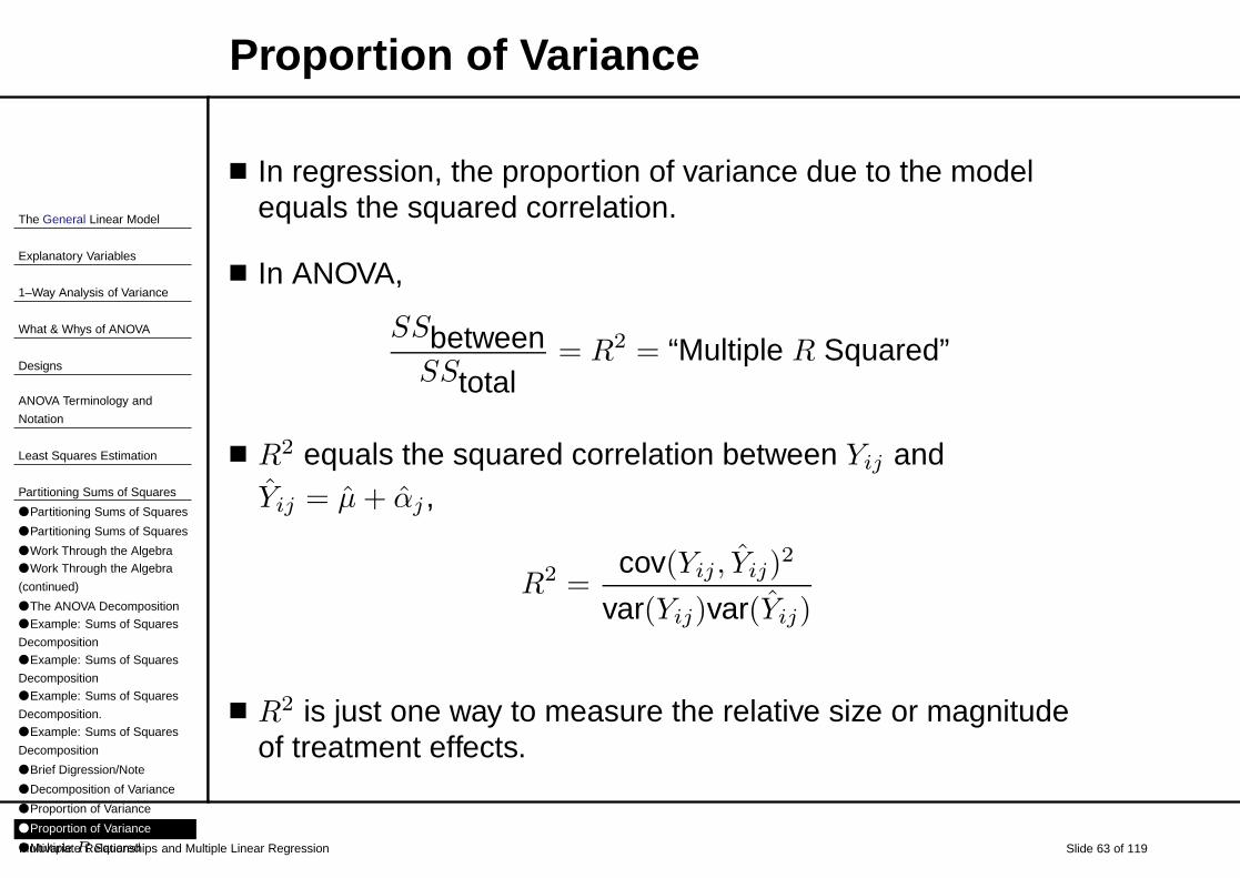
Proportion of Variance
■ In regression, the proportion of variance due to the modelequals the squared correlation.
■ In ANOVA,
SSbetweenSStotal
= R2 = “Multiple R Squared”
■ R2 equals the squared correlation between Yij andYij = µ + αj ,
R2 =cov(Yij , Yij)
2
var(Yij)var(Yij)
■ R2 is just one way to measure the relative size or magnitudeof treatment effects.

The General Linear Model
Explanatory Variables
1–Way Analysis of Variance
What & Whys of ANOVA
Designs
ANOVA Terminology and
Notation
Least Squares Estimation
Partitioning Sums of Squares
● Partitioning Sums of Squares
● Partitioning Sums of Squares
● Work Through the Algebra● Work Through the Algebra
(continued)
● The ANOVA Decomposition
● Example: Sums of Squares
Decomposition
● Example: Sums of Squares
Decomposition
● Example: Sums of Squares
Decomposition.
● Example: Sums of Squares
Decomposition
● Brief Digression/Note
● Decomposition of Variance
● Proportion of Variance
● Proportion of Variance
● Multiple R Squared
Hypothesis Testing: F -test
Multivariate Relationships and Multiple Linear Regression Slide 64 of 119
Multiple R Squared
■ In Wiley & Voss example,
SSbetweenSStotal
= R2 =1, 142.188
10, 998.414= .1039
and r(Yij , Yij) =√
.1039 = .322
■ 1 − R2 is proportional to the “loss function”, which we set outto minimize,
1 − R2 = 1 − .1039 = .8961
■ Is this statistically a good model?

The General Linear Model
Explanatory Variables
1–Way Analysis of Variance
What & Whys of ANOVA
Designs
ANOVA Terminology and
Notation
Least Squares Estimation
Partitioning Sums of Squares
Hypothesis Testing: F -test
● Hypothesis Testing: F -test
● Assumptions:
● Test Statistic
● Test Statistic (continued)
● Test Statistic: Variance
Estimates● Test Statistic: Variance
Estimates● Test Statistic: Variance
Estimates
● Variation Due to Treatments● Variation Due to Treatments
(continued)● Variation Due to Treatments
(continued)● Variation Due to Treatments
(continued)
● Test Statistic: Variance
Estimates
Multivariate Relationships and Multiple Linear Regression Slide 65 of 119
Hypothesis Testing: F -test
■ Statistical Hypotheses:
Ho : µ1 = µ2 = . . . = µJ or all µ′js are equal
Ha : at least one µ′js is not equal to the rest
or Ha : the means differ in the population
■ The alternative hypothesis is NOT
µ1 6= µ2 6= . . . 6= µJ
The General Linear Model
Explanatory Variables
1–Way Analysis of Variance
What & Whys of ANOVA
Designs
ANOVA Terminology and
Notation
Least Squares Estimation
Partitioning Sums of Squares
Hypothesis Testing: F -test
● Hypothesis Testing: F -test
● Assumptions:
● Test Statistic
● Test Statistic (continued)
● Test Statistic: Variance
Estimates● Test Statistic: Variance
Estimates● Test Statistic: Variance
Estimates
● Variation Due to Treatments● Variation Due to Treatments
(continued)● Variation Due to Treatments
(continued)● Variation Due to Treatments
(continued)
● Test Statistic: Variance
Estimates
Multivariate Relationships and Multiple Linear Regression Slide 66 of 119
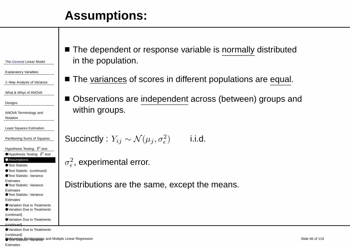
Assumptions:
■ The dependent or response variable is normally distributedin the population.
■ The variances of scores in different populations are equal.
■ Observations are independent across (between) groups andwithin groups.
Succinctly : Yij ∼ N (µj , σ2ǫ ) i.i.d.
σ2ǫ , experimental error.
Distributions are the same, except the means.

The General Linear Model
Explanatory Variables
1–Way Analysis of Variance
What & Whys of ANOVA
Designs
ANOVA Terminology and
Notation
Least Squares Estimation
Partitioning Sums of Squares
Hypothesis Testing: F -test
● Hypothesis Testing: F -test
● Assumptions:
● Test Statistic
● Test Statistic (continued)
● Test Statistic: Variance
Estimates● Test Statistic: Variance
Estimates● Test Statistic: Variance
Estimates
● Variation Due to Treatments● Variation Due to Treatments
(continued)● Variation Due to Treatments
(continued)● Variation Due to Treatments
(continued)
● Test Statistic: Variance
Estimates
Multivariate Relationships and Multiple Linear Regression Slide 67 of 119
Test Statistic
■ If Ho is TRUE, then we expect the sample means to differbecause of unsystematic error, i.e., σ2
ǫ .
■ If Ho is FALSE, then the differences between sample meansreflect
1. Experimental or unsystematic error, i.e., σ2ǫ
2. Systematic differences or true differences betweenpopulation means, or “treatment effects”.

The General Linear Model
Explanatory Variables
1–Way Analysis of Variance
What & Whys of ANOVA
Designs
ANOVA Terminology and
Notation
Least Squares Estimation
Partitioning Sums of Squares
Hypothesis Testing: F -test
● Hypothesis Testing: F -test
● Assumptions:
● Test Statistic
● Test Statistic (continued)
● Test Statistic: Variance
Estimates● Test Statistic: Variance
Estimates● Test Statistic: Variance
Estimates
● Variation Due to Treatments● Variation Due to Treatments
(continued)● Variation Due to Treatments
(continued)● Variation Due to Treatments
(continued)
● Test Statistic: Variance
Estimates
Multivariate Relationships and Multiple Linear Regression Slide 68 of 119
Test Statistic (continued)
■ To test Ho, we look at the following ratio:
(Differences among treatment means)
(Differences among subjects treated alike)
(Between group differences)
(Within group differences)
■ If Ho is TRUE, then this ratio equals
(Experimental Error)(Experimental Error)
∼ 1
■ If Ho is FALSE, then this ratio equals
(Treatment Effects) + (Experimental Error)(Experimental Error)
> 1

The General Linear Model
Explanatory Variables
1–Way Analysis of Variance
What & Whys of ANOVA
Designs
ANOVA Terminology and
Notation
Least Squares Estimation
Partitioning Sums of Squares
Hypothesis Testing: F -test
● Hypothesis Testing: F -test
● Assumptions:
● Test Statistic
● Test Statistic (continued)
● Test Statistic: Variance
Estimates● Test Statistic: Variance
Estimates● Test Statistic: Variance
Estimates
● Variation Due to Treatments● Variation Due to Treatments
(continued)● Variation Due to Treatments
(continued)● Variation Due to Treatments
(continued)
● Test Statistic: Variance
Estimates
Multivariate Relationships and Multiple Linear Regression Slide 69 of 119
Test Statistic: Variance Estimates
■ How to estimate σ2ǫ ? (The denominator of our test statistic).
■ Use all the data and compute a pooled estimate.
σ2pool =
(n1 − 1)s21 + (n2 − 1)s2
2 + . . . + (nJ − 1)s2J
(n1 − 1) + (n2 − 1) + . . . + (nJ − 1)
=
∑Jj=1
∑nj
i=1(Yij − Yj)2
∑Jj=1(nj − 1)
=SSwithin
∑Jj=1(nj − 1)
∑Jj=1(nj − 1) equals the degrees of freedom associated with
σ2pool; that is, νpool.

The General Linear Model
Explanatory Variables
1–Way Analysis of Variance
What & Whys of ANOVA
Designs
ANOVA Terminology and
Notation
Least Squares Estimation
Partitioning Sums of Squares
Hypothesis Testing: F -test
● Hypothesis Testing: F -test
● Assumptions:
● Test Statistic
● Test Statistic (continued)
● Test Statistic: Variance
Estimates● Test Statistic: Variance
Estimates● Test Statistic: Variance
Estimates
● Variation Due to Treatments● Variation Due to Treatments
(continued)● Variation Due to Treatments
(continued)● Variation Due to Treatments
(continued)
● Test Statistic: Variance
Estimates
Multivariate Relationships and Multiple Linear Regression Slide 70 of 119
Test Statistic: Variance Estimates
■ The pooled variance, SSw
νw= MSw = σ2
ǫ is thewithin groups mean squared error.
■ Degrees of freedom= νw =∑J
j=1(nj − 1), which equals(N − J) for a balanced design.
■ MSw is also called
◆ Error mean square
◆ Mean square error
◆ Residual mean square
■ Wiley & Voss example: MSw = 9, 856.250/(64− 4) = 164.271

The General Linear Model
Explanatory Variables
1–Way Analysis of Variance
What & Whys of ANOVA
Designs
ANOVA Terminology and
Notation
Least Squares Estimation
Partitioning Sums of Squares
Hypothesis Testing: F -test
● Hypothesis Testing: F -test
● Assumptions:
● Test Statistic
● Test Statistic (continued)
● Test Statistic: Variance
Estimates● Test Statistic: Variance
Estimates● Test Statistic: Variance
Estimates
● Variation Due to Treatments● Variation Due to Treatments
(continued)● Variation Due to Treatments
(continued)● Variation Due to Treatments
(continued)
● Test Statistic: Variance
Estimates
Multivariate Relationships and Multiple Linear Regression Slide 71 of 119
Test Statistic: Variance Estimates
SSw
νw= MSw = σ2
ǫ
■ The expected value E(SSw/νw) = MSw = σ2ǫ
■ It does not depend on whether Ho is true or false.
■ It is constant across groups
■ In a good experiment or study, this should be “small” andonly reflect chance error.

The General Linear Model
Explanatory Variables
1–Way Analysis of Variance
What & Whys of ANOVA
Designs
ANOVA Terminology and
Notation
Least Squares Estimation
Partitioning Sums of Squares
Hypothesis Testing: F -test
● Hypothesis Testing: F -test
● Assumptions:
● Test Statistic
● Test Statistic (continued)
● Test Statistic: Variance
Estimates● Test Statistic: Variance
Estimates● Test Statistic: Variance
Estimates
● Variation Due to Treatments● Variation Due to Treatments
(continued)● Variation Due to Treatments
(continued)● Variation Due to Treatments
(continued)
● Test Statistic: Variance
Estimates
Multivariate Relationships and Multiple Linear Regression Slide 72 of 119
Variation Due to Treatments
Consider the sampling distributions of the means for each ofour treatments.. . .
Sample Population VarianceGroup Mean (true) mean of Yj
N Y1 µ1 σ2Y1
= σ2ǫ /n1
E Y2 µ2 σ2Y2
= σ2ǫ /n2
S Y3 µ3 σ2Y3
= σ2ǫ /n3
A Y4 µ4 σ2Y4
= σ2ǫ /n4
In Wiley & Voss example, we have a “balanced design”; that is,n1 = n2 = n3 = n4 = 16 (equal sample sizes).

The General Linear Model
Explanatory Variables
1–Way Analysis of Variance
What & Whys of ANOVA
Designs
ANOVA Terminology and
Notation
Least Squares Estimation
Partitioning Sums of Squares
Hypothesis Testing: F -test
● Hypothesis Testing: F -test
● Assumptions:
● Test Statistic
● Test Statistic (continued)
● Test Statistic: Variance
Estimates● Test Statistic: Variance
Estimates● Test Statistic: Variance
Estimates
● Variation Due to Treatments● Variation Due to Treatments
(continued)● Variation Due to Treatments
(continued)● Variation Due to Treatments
(continued)
● Test Statistic: Variance
Estimates
Multivariate Relationships and Multiple Linear Regression Slide 73 of 119
Variation Due to Treatments (continued)For balanced designs,
If Ho : µ1 = µ2 = µ3 = µ4 = µ (a constant) is true,
Then Y1, Y2, . . . YJ is a random sample from the population ofsample means of size J with mean µ and variance σ2
ǫ /n.
■ The grand mean
Y =1
N
J∑
j=1
n∑
i=1
Y ij
where N =∑J
j=1 nj .
■ If Ho is true, then variance of the means,
σ2Yj
=1
(J − 1)
J∑
j=1
(Yj − Y )2

The General Linear Model
Explanatory Variables
1–Way Analysis of Variance
What & Whys of ANOVA
Designs
ANOVA Terminology and
Notation
Least Squares Estimation
Partitioning Sums of Squares
Hypothesis Testing: F -test
● Hypothesis Testing: F -test
● Assumptions:
● Test Statistic
● Test Statistic (continued)
● Test Statistic: Variance
Estimates● Test Statistic: Variance
Estimates● Test Statistic: Variance
Estimates
● Variation Due to Treatments● Variation Due to Treatments
(continued)● Variation Due to Treatments
(continued)● Variation Due to Treatments
(continued)
● Test Statistic: Variance
Estimates
Multivariate Relationships and Multiple Linear Regression Slide 74 of 119
Variation Due to Treatments (continued)
For balanced designs, If Ho is true
■ Then variance of the means (by definition),
σ2Yj
=1
(J − 1)
J∑
j=1
(Yj − Y )2
■ Since σ2Yj
= σ2ǫ /n, the estimate of σ2
ǫ is
σ2ǫ = nσ2
Yj=
1
(J − 1)
J∑
j=1
n(Yj − Y )2
=SSbetween
(J − 1)
= MSbetween

The General Linear Model
Explanatory Variables
1–Way Analysis of Variance
What & Whys of ANOVA
Designs
ANOVA Terminology and
Notation
Least Squares Estimation
Partitioning Sums of Squares
Hypothesis Testing: F -test
● Hypothesis Testing: F -test
● Assumptions:
● Test Statistic
● Test Statistic (continued)
● Test Statistic: Variance
Estimates● Test Statistic: Variance
Estimates● Test Statistic: Variance
Estimates
● Variation Due to Treatments● Variation Due to Treatments
(continued)● Variation Due to Treatments
(continued)● Variation Due to Treatments
(continued)
● Test Statistic: Variance
Estimates
Multivariate Relationships and Multiple Linear Regression Slide 75 of 119
Variation Due to Treatments (continued)
For unbalanced designs,
■ Grand mean,
Y =1
N
J∑
j=1
nj∑
i=1
Y ij
where N =∑J
j=1 nj .
■ Estimate of σ2ǫ if Ho is true,
σ2ǫ = =
1
(J − 1)
J∑
j=1
nj(Yj − Y )2
=SSbetween
(J − 1)= MSbetween
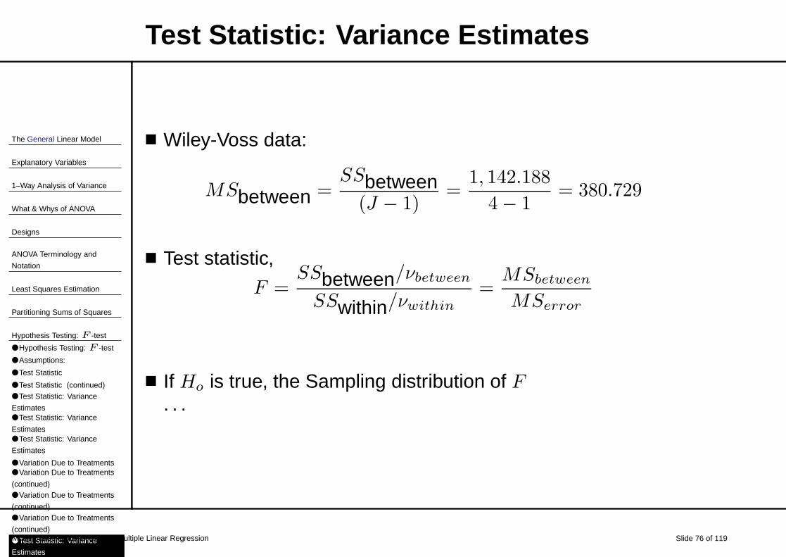
The General Linear Model
Explanatory Variables
1–Way Analysis of Variance
What & Whys of ANOVA
Designs
ANOVA Terminology and
Notation
Least Squares Estimation
Partitioning Sums of Squares
Hypothesis Testing: F -test
● Hypothesis Testing: F -test
● Assumptions:
● Test Statistic
● Test Statistic (continued)
● Test Statistic: Variance
Estimates● Test Statistic: Variance
Estimates● Test Statistic: Variance
Estimates
● Variation Due to Treatments● Variation Due to Treatments
(continued)● Variation Due to Treatments
(continued)● Variation Due to Treatments
(continued)
● Test Statistic: Variance
Estimates
Multivariate Relationships and Multiple Linear Regression Slide 76 of 119
Test Statistic: Variance Estimates
■ Wiley-Voss data:
MSbetween =SSbetween
(J − 1)=
1, 142.188
4 − 1= 380.729
■ Test statistic,
F =SSbetween/νbetween
SSwithin/νwithin=
MSbetween
MSerror
■ If Ho is true, the Sampling distribution of F. . .

The General Linear Model
Explanatory Variables
1–Way Analysis of Variance
What & Whys of ANOVA
Designs
ANOVA Terminology and
Notation
Least Squares Estimation
Partitioning Sums of Squares
Hypothesis Testing: F -test
● Hypothesis Testing: F -test
● Assumptions:
● Test Statistic
● Test Statistic (continued)
● Test Statistic: Variance
Estimates● Test Statistic: Variance
Estimates● Test Statistic: Variance
Estimates
● Variation Due to Treatments● Variation Due to Treatments
(continued)● Variation Due to Treatments
(continued)● Variation Due to Treatments
(continued)
● Test Statistic: Variance
Estimates
Multivariate Relationships and Multiple Linear Regression Slide 77 of 119
Sampling distribution of F
If Ho is true, the Sampling distribution of F. . .
F =SSbetween/νbetween
SSwithin/νwithin
1σ2
ǫ
1σ2
ǫ
=
Jj=1
nj(Yj−Y )2/σ2
ǫ
(J−1)
Jj=1
nji=1
(Yij−Yj)2/σ2ǫ
Jj=1
(nj−1)
=χ2
b/νb
χ2w/νw
∼ Fνb,νw

The General Linear Model
Explanatory Variables
1–Way Analysis of Variance
What & Whys of ANOVA
Designs
ANOVA Terminology and
Notation
Least Squares Estimation
Partitioning Sums of Squares
Hypothesis Testing: F -test
● Hypothesis Testing: F -test
● Assumptions:
● Test Statistic
● Test Statistic (continued)
● Test Statistic: Variance
Estimates● Test Statistic: Variance
Estimates● Test Statistic: Variance
Estimates
● Variation Due to Treatments● Variation Due to Treatments
(continued)● Variation Due to Treatments
(continued)● Variation Due to Treatments
(continued)
● Test Statistic: Variance
Estimates
Multivariate Relationships and Multiple Linear Regression Slide 78 of 119
ANOVA Summary Table
■ For Wiley-Voss exampleSource df SS MS F p-value
Instructions 3 1,142.188 380.729 2.32 .08Error 60 9,856.250 164.271
Total 63 10,998.414
■ Retain Ho, because p-value= (1 − .0.92) = .08 > α = .05
■ If we had rejected Ho, what would you want to know?

The General Linear Model
Explanatory Variables
1–Way Analysis of Variance
What & Whys of ANOVA
Designs
ANOVA Terminology and
Notation
Least Squares Estimation
Partitioning Sums of Squares
Hypothesis Testing: F -test
● Hypothesis Testing: F -test
● Assumptions:
● Test Statistic
● Test Statistic (continued)
● Test Statistic: Variance
Estimates● Test Statistic: Variance
Estimates● Test Statistic: Variance
Estimates
● Variation Due to Treatments● Variation Due to Treatments
(continued)● Variation Due to Treatments
(continued)● Variation Due to Treatments
(continued)
● Test Statistic: Variance
Estimates
Multivariate Relationships and Multiple Linear Regression Slide 79 of 119
One-Factor ANOVA Summary Table■ In general, for 1 factor ANOVA
Source df SS MS F
Factor A J − 1jnj(Yj − Y )2 SSA
νA
MSA
MSerror
Errorj(nj − 1)
j i(Yij − Yj)
2 SSerror
νerror
Total N − 1j i
(Yij − Y )2
■ Reject Ho for “large” F statistics. Compare to Fν1,ν2
distribution.
■ By “Total”, we mean “total corrected for mean”
■ The terms “Factor A”, “Treatment”, “Condition”, “Between”are interchangeable.
■ The terms “within”, “residual” and “error” areinterchangeable.

The General Linear Model
Explanatory Variables
1–Way Analysis of Variance
What & Whys of ANOVA
Designs
ANOVA Terminology and
Notation
Least Squares Estimation
Partitioning Sums of Squares
Hypothesis Testing: F -test
● Hypothesis Testing: F -test
● Assumptions:
● Test Statistic
● Test Statistic (continued)
● Test Statistic: Variance
Estimates● Test Statistic: Variance
Estimates● Test Statistic: Variance
Estimates
● Variation Due to Treatments● Variation Due to Treatments
(continued)● Variation Due to Treatments
(continued)● Variation Due to Treatments
(continued)
● Test Statistic: Variance
Estimates
Multivariate Relationships and Multiple Linear Regression Slide 80 of 119
A Closer Look at MSbetween
■ If Ho is TRUE, then
E(MSbetween) = σ2ǫ
■ IF Ho is FALSE (i.e., Ha is true), then the Expected value
E(MSbetween) = σ2ǫ +
∑Jj=1 njα
2j
J − 1
(See Hayes for proof).

The General Linear Model
Explanatory Variables
1–Way Analysis of Variance
What & Whys of ANOVA
Designs
ANOVA Terminology and
Notation
Least Squares Estimation
Partitioning Sums of Squares
Hypothesis Testing: F -test
● Hypothesis Testing: F -test
● Assumptions:
● Test Statistic
● Test Statistic (continued)
● Test Statistic: Variance
Estimates● Test Statistic: Variance
Estimates● Test Statistic: Variance
Estimates
● Variation Due to Treatments● Variation Due to Treatments
(continued)● Variation Due to Treatments
(continued)● Variation Due to Treatments
(continued)
● Test Statistic: Variance
Estimates
Multivariate Relationships and Multiple Linear Regression Slide 81 of 119
A Closer Look at the F Statistic
■ If Ho is true:
F =MSbetween
MSerror=
σ2ǫ
σ2ǫ
■ If Ho is false:
F =MSbetween
MSerror=
σ2ǫ +
Jj=1
njα2
j
J−1
σ2ǫ
■ Test statistic F = MSbetween/MSerror follows a non-centralF distribution.

The General Linear Model
Explanatory Variables
1–Way Analysis of Variance
What & Whys of ANOVA
Designs
ANOVA Terminology and
Notation
Least Squares Estimation
Partitioning Sums of Squares
Hypothesis Testing: F -test
● Hypothesis Testing: F -test
● Assumptions:
● Test Statistic
● Test Statistic (continued)
● Test Statistic: Variance
Estimates● Test Statistic: Variance
Estimates● Test Statistic: Variance
Estimates
● Variation Due to Treatments● Variation Due to Treatments
(continued)● Variation Due to Treatments
(continued)● Variation Due to Treatments
(continued)
● Test Statistic: Variance
Estimates
Multivariate Relationships and Multiple Linear Regression Slide 82 of 119
A Summary of 1-Factor ANOVA■ Statistical Hypotheses: Ho : µ1 = µ2 = . . . = µJ or
Ho : α1 = α2 = . . . = αJ versusHa: at least one µj (or αj) differs from rest.
■ Assumptions: Yij ∼ N (µj , σ2ǫ ) i.i.d.(or write out model).
■ Test Statistic:
Source df SS MS F
Between (J − 1) J
j=1nj(Yj − Y )2 SSb
νB
MSB
MSw
Within J
j=1(nj − 1) 2
j=1
nj
i=1(Yij − Yj)
2 SSw
νw
Total (corrected) N − 1 J
j=1
nj
i=1(Yij − Y )2
■ Sampling distribution: If the null hypothesis is true, thenF ∼ (central) Fνb,νw
distribution.
■ Decision and Conclusion: If you reject the Ho all we know isthat at least one group has a mean that’s different from therest.

The General Linear Model
Explanatory Variables
1–Way Analysis of Variance
What & Whys of ANOVA
Designs
ANOVA Terminology and
Notation
Least Squares Estimation
Partitioning Sums of Squares
Hypothesis Testing: F -test
ANOVA & SAS
● ANOVA & SAS
● SAS/ASSIST
● SAS/Program Commands
● SAS/Analyst
Unequal Sample Sizes
Effect Size
Power
Violations of Assumptions
Multivariate Relationships and Multiple Linear Regression Slide 83 of 119
ANOVA & SAS
■ ASSIST■ Analyst■ Program Commands

The General Linear Model
Explanatory Variables
1–Way Analysis of Variance
What & Whys of ANOVA
Designs
ANOVA Terminology and
Notation
Least Squares Estimation
Partitioning Sums of Squares
Hypothesis Testing: F -test
ANOVA & SAS
● ANOVA & SAS
● SAS/ASSIST
● SAS/Program Commands
● SAS/Analyst
Unequal Sample Sizes
Effect Size
Power
Violations of Assumptions
Multivariate Relationships and Multiple Linear Regression Slide 84 of 119
SAS/ASSIST
■ Put a data set in SAS working memory■ On main toolbar: Solutions
> ASSIST> Data Analysis
> ANOVA> Analysis of Variance
■ In ANOVA window, fill in◆ Table −→ data set,◆ Dependent −→ dependent variable◆ Classification −→ factor
■ Click on RUN.

The General Linear Model
Explanatory Variables
1–Way Analysis of Variance
What & Whys of ANOVA
Designs
ANOVA Terminology and
Notation
Least Squares Estimation
Partitioning Sums of Squares
Hypothesis Testing: F -test
ANOVA & SAS
● ANOVA & SAS
● SAS/ASSIST
● SAS/Program Commands
● SAS/Analyst
Unequal Sample Sizes
Effect Size
Power
Violations of Assumptions
Multivariate Relationships and Multiple Linear Regression Slide 85 of 119
SAS/Program Commands
■ In the program/text editor window:
PROC GLM DATA=ivt;CLASS instruct;MODEL ivt = instruct;TITLE ’ANOVA for 1-factor Wiley & Voss’;
RUN;■ Click on RUN on the toolbar■ Note: This is what SAS/ASSIST does.

The General Linear Model
Explanatory Variables
1–Way Analysis of Variance
What & Whys of ANOVA
Designs
ANOVA Terminology and
Notation
Least Squares Estimation
Partitioning Sums of Squares
Hypothesis Testing: F -test
ANOVA & SAS
● ANOVA & SAS
● SAS/ASSIST
● SAS/Program Commands
● SAS/Analyst
Unequal Sample Sizes
Effect Size
Power
Violations of Assumptions
Multivariate Relationships and Multiple Linear Regression Slide 86 of 119
SAS/Analyst
■ Have a data set in working memory.■ On SAS main toolbar:→Solutions → Analysis → Analyst
■ In Analyst environment, File > Open by SAS name“WORK” −→ select the one you want.
■ On Analyst toolbar:→ Statistics → ANOVA → 1 Way ANOVA
■ fill in boxes with dependent and independent variable names.■ Request any other options you want.■ Click “OK”.

The General Linear Model
Explanatory Variables
1–Way Analysis of Variance
What & Whys of ANOVA
Designs
ANOVA Terminology and
Notation
Least Squares Estimation
Partitioning Sums of Squares
Hypothesis Testing: F -test
ANOVA & SAS
Unequal Sample Sizes
● Unequal Sample Sizes
● The Data
● The Data and Means
● Summary Statistics
● ANOVA Summary Table
● Plot of The Means±2sY
Effect Size
Power
Violations of AssumptionsMultivariate Relationships and Multiple Linear Regression Slide 87 of 119
Unequal Sample Sizes
■ Example: Data are from Moore & McCabe who got it fromKirmani, A & Wright, P. (1989). Money Talks: PerceivedAdvertising expense and expected product quality. Journal ofConsumer Research, 16, 344-353.
■ Yij = rating of the quality of a take-home refrigeratedentrees based on add from 1 (bad) to 7 (good).
■ Factor: Information included in the add:
◆ U: Undermine quality and advertising (n1 = 55)
◆ A: Affirm quality and advertising (n2 = 36)
◆ C: Control (n3 = 36)

The General Linear Model
Explanatory Variables
1–Way Analysis of Variance
What & Whys of ANOVA
Designs
ANOVA Terminology and
Notation
Least Squares Estimation
Partitioning Sums of Squares
Hypothesis Testing: F -test
ANOVA & SAS
Unequal Sample Sizes
● Unequal Sample Sizes
● The Data
● The Data and Means
● Summary Statistics
● ANOVA Summary Table
● Plot of The Means±2sY
Effect Size
Power
Violations of AssumptionsMultivariate Relationships and Multiple Linear Regression Slide 88 of 119
The Data

The General Linear Model
Explanatory Variables
1–Way Analysis of Variance
What & Whys of ANOVA
Designs
ANOVA Terminology and
Notation
Least Squares Estimation
Partitioning Sums of Squares
Hypothesis Testing: F -test
ANOVA & SAS
Unequal Sample Sizes
● Unequal Sample Sizes
● The Data
● The Data and Means
● Summary Statistics
● ANOVA Summary Table
● Plot of The Means±2sY
Effect Size
Power
Violations of AssumptionsMultivariate Relationships and Multiple Linear Regression Slide 89 of 119
The Data and Means

The General Linear Model
Explanatory Variables
1–Way Analysis of Variance
What & Whys of ANOVA
Designs
ANOVA Terminology and
Notation
Least Squares Estimation
Partitioning Sums of Squares
Hypothesis Testing: F -test
ANOVA & SAS
Unequal Sample Sizes
● Unequal Sample Sizes
● The Data
● The Data and Means
● Summary Statistics
● ANOVA Summary Table
● Plot of The Means±2sY
Effect Size
Power
Violations of AssumptionsMultivariate Relationships and Multiple Linear Regression Slide 90 of 119
Summary Statistics
Group N Mean Std Dev Variance
A 36 5.0555556 0.8261596 0.6825397C 36 5.4166667 0.8742344 0.7642857U 55 4.5090909 0.6904837 0.4767677
Total 127 4.9212598 0.8692845 0.7556555
SStotal = (J − 1)s2 = (127 − 1)(.7556555) = 95.2125
SSerror = (n1 − 1)s21 + (n2 − 1)s2
2 + (n3 − 1)s23
= (36 − 1)(.6825397) + (36 − 1)(.7642857)
+(55 − 1)(.4767677)
= 76.3843
SSgroup = SStotal − SSerror= 95.2125 − 76.3843 = 18.8282

The General Linear Model
Explanatory Variables
1–Way Analysis of Variance
What & Whys of ANOVA
Designs
ANOVA Terminology and
Notation
Least Squares Estimation
Partitioning Sums of Squares
Hypothesis Testing: F -test
ANOVA & SAS
Unequal Sample Sizes
● Unequal Sample Sizes
● The Data
● The Data and Means
● Summary Statistics
● ANOVA Summary Table
● Plot of The Means±2sY
Effect Size
Power
Violations of AssumptionsMultivariate Relationships and Multiple Linear Regression Slide 91 of 119
ANOVA Summary Table
Basically what get from SAS
Sum of MeanSource DF Squares Square F Pr > F
Model 2 18.828 9.414 15.28 < .0001
Error 124 76.384 0.616
Corrected Total 126 95.213
R-Square Coeff Var Root MSE qual Mean
0.197750 15.94832 0.784858 4.921260

The General Linear Model
Explanatory Variables
1–Way Analysis of Variance
What & Whys of ANOVA
Designs
ANOVA Terminology and
Notation
Least Squares Estimation
Partitioning Sums of Squares
Hypothesis Testing: F -test
ANOVA & SAS
Unequal Sample Sizes
● Unequal Sample Sizes
● The Data
● The Data and Means
● Summary Statistics
● ANOVA Summary Table
● Plot of The Means±2sY
Effect Size
Power
Violations of AssumptionsMultivariate Relationships and Multiple Linear Regression Slide 92 of 119
Plot of The Means ±2sY

The General Linear Model
Explanatory Variables
1–Way Analysis of Variance
What & Whys of ANOVA
Designs
ANOVA Terminology and
Notation
Least Squares Estimation
Partitioning Sums of Squares
Hypothesis Testing: F -test
ANOVA & SAS
Unequal Sample Sizes
Effect Size
● Effect Size
● Effect Size
● Effect Size: Omega Squared
● Properties of Omega Squared
● Epsilon Squared, e2
● Notes on Effect Size
Measures
Power
Violations of AssumptionsMultivariate Relationships and Multiple Linear Regression Slide 93 of 119
Effect Size
Effect Size: Estimates of treatment magnitude
■ p-value of F -statistic is not a measure of size of an effect.
■ Goal: develop comprehensive theory of a phenomenon.
◆ The importance of an experimental manipulation −→degree to which can account for total variability amongsubjects by isolating experimental effect.
◆ In observational studies, the importance of factors −→degree to which differences can be explained by factors.

The General Linear Model
Explanatory Variables
1–Way Analysis of Variance
What & Whys of ANOVA
Designs
ANOVA Terminology and
Notation
Least Squares Estimation
Partitioning Sums of Squares
Hypothesis Testing: F -test
ANOVA & SAS
Unequal Sample Sizes
Effect Size
● Effect Size
● Effect Size
● Effect Size: Omega Squared
● Properties of Omega Squared
● Epsilon Squared, e2
● Notes on Effect Size
Measures
Power
Violations of AssumptionsMultivariate Relationships and Multiple Linear Regression Slide 94 of 119
Effect Size
Estimates of treatment magnitude
■ Multiple R2 = SSbetween/SStotal
■ Omega squared, ω2.
■ Epsilon squared, e2.
■ Non-centrality parameter.

The General Linear Model
Explanatory Variables
1–Way Analysis of Variance
What & Whys of ANOVA
Designs
ANOVA Terminology and
Notation
Least Squares Estimation
Partitioning Sums of Squares
Hypothesis Testing: F -test
ANOVA & SAS
Unequal Sample Sizes
Effect Size
● Effect Size
● Effect Size
● Effect Size: Omega Squared
● Properties of Omega Squared
● Epsilon Squared, e2
● Notes on Effect Size
Measures
Power
Violations of AssumptionsMultivariate Relationships and Multiple Linear Regression Slide 95 of 119
Effect Size: Omega Squared
ω2 =variance due to treatment
total variance
=
∑Jj=1 α2
j/J
σ2ǫ +
∑Jj=1 α2
j/J
■ Most common effect size measure.
■ The proportion of total population variance due to (explainedby) treatments.
■ Estimating ω2,
ω2 =SSbetween − (J − 1)MSerror
SStotal + MSerror
◆ SSbetween reflects treatment magnitude and σ2ǫ .
◆ MSerror only reflects σ2ǫ .
◆ There are other algebraically equivalent formula’s — thisone easiest to compute but obscures logic.
◆ Quality rating data: ω2 = 18.828−(3−1)(.616)95.213+.616 = .18

The General Linear Model
Explanatory Variables
1–Way Analysis of Variance
What & Whys of ANOVA
Designs
ANOVA Terminology and
Notation
Least Squares Estimation
Partitioning Sums of Squares
Hypothesis Testing: F -test
ANOVA & SAS
Unequal Sample Sizes
Effect Size
● Effect Size
● Effect Size
● Effect Size: Omega Squared
● Properties of Omega Squared
● Epsilon Squared, e2
● Notes on Effect Size
Measures
Power
Violations of AssumptionsMultivariate Relationships and Multiple Linear Regression Slide 96 of 119
Properties of Omega Squared
■ 0 < ω2 < 1.00 (unless F statistic < 1).
■ For social science research, Cohen (Keppel, 1982) suggests
◆ “Large” −→ ω2 > .15
◆ “Medium”−→ ω2 ≈ .06
◆ “Small”−→ ω2 ≈ .01
■ ω2 is not a test statistic, but a significant F statistics impliesthat ω2 is “significantly” greater than 0.

The General Linear Model
Explanatory Variables
1–Way Analysis of Variance
What & Whys of ANOVA
Designs
ANOVA Terminology and
Notation
Least Squares Estimation
Partitioning Sums of Squares
Hypothesis Testing: F -test
ANOVA & SAS
Unequal Sample Sizes
Effect Size
● Effect Size
● Effect Size
● Effect Size: Omega Squared
● Properties of Omega Squared
● Epsilon Squared, e2
● Notes on Effect Size
Measures
Power
Violations of AssumptionsMultivariate Relationships and Multiple Linear Regression Slide 97 of 119
Epsilon Squared, e2
e2 =SSbetween − (J − 1)MSerror
SStotal
■ e2 > ω2 because of difference in denominators.
■ Quality rating data:
e2 = (18.828 − (3 − 1))(.616)/95.213 = .185.
■ In a “good” experiment, difference between e2 and ω2 shouldbe small, i.e.,
MSerrorσ2ǫ
is small.

The General Linear Model
Explanatory Variables
1–Way Analysis of Variance
What & Whys of ANOVA
Designs
ANOVA Terminology and
Notation
Least Squares Estimation
Partitioning Sums of Squares
Hypothesis Testing: F -test
ANOVA & SAS
Unequal Sample Sizes
Effect Size
● Effect Size
● Effect Size
● Effect Size: Omega Squared
● Properties of Omega Squared
● Epsilon Squared, e2
● Notes on Effect Size
Measures
Power
Violations of AssumptionsMultivariate Relationships and Multiple Linear Regression Slide 98 of 119
Notes on Effect Size Measures
■ e2 comes out of multiple regression framework.
■ R2 > e2 because e2 is obtainable from “adjusted” or“shrunken” R2.
■ ω2 ≤ e2 ≤ R2. For quality rating data:
ω2 = .184 < e2 = .185 < R2 = .198
■ e2 is a better estimate of the strength in the population thanR2.
■ For simple designs, can use either ω2 or e2.
■ ω2 has been extended to more complex designs.

The General Linear Model
Explanatory Variables
1–Way Analysis of Variance
What & Whys of ANOVA
Designs
ANOVA Terminology and
Notation
Least Squares Estimation
Partitioning Sums of Squares
Hypothesis Testing: F -test
ANOVA & SAS
Unequal Sample Sizes
Effect Size
Power
● Power
● Power● Example: Non-Centrality
Parameter
● Things that Effect Power
● Things that Effect Power
(continued)
● Main Sources of Error
Variance● Main Sources of Error
Variance
Multivariate Relationships and Multiple Linear Regression Slide 99 of 119
Power
The decision of a hypothesis test will either be correct orincorrect.
Possible Outcomes:Actual State of World
Ho true Ha trueretain Ho correct Type II error
Decision 1 − α β
reject Ho Type I error Correctα Power= 1 − β
1 1
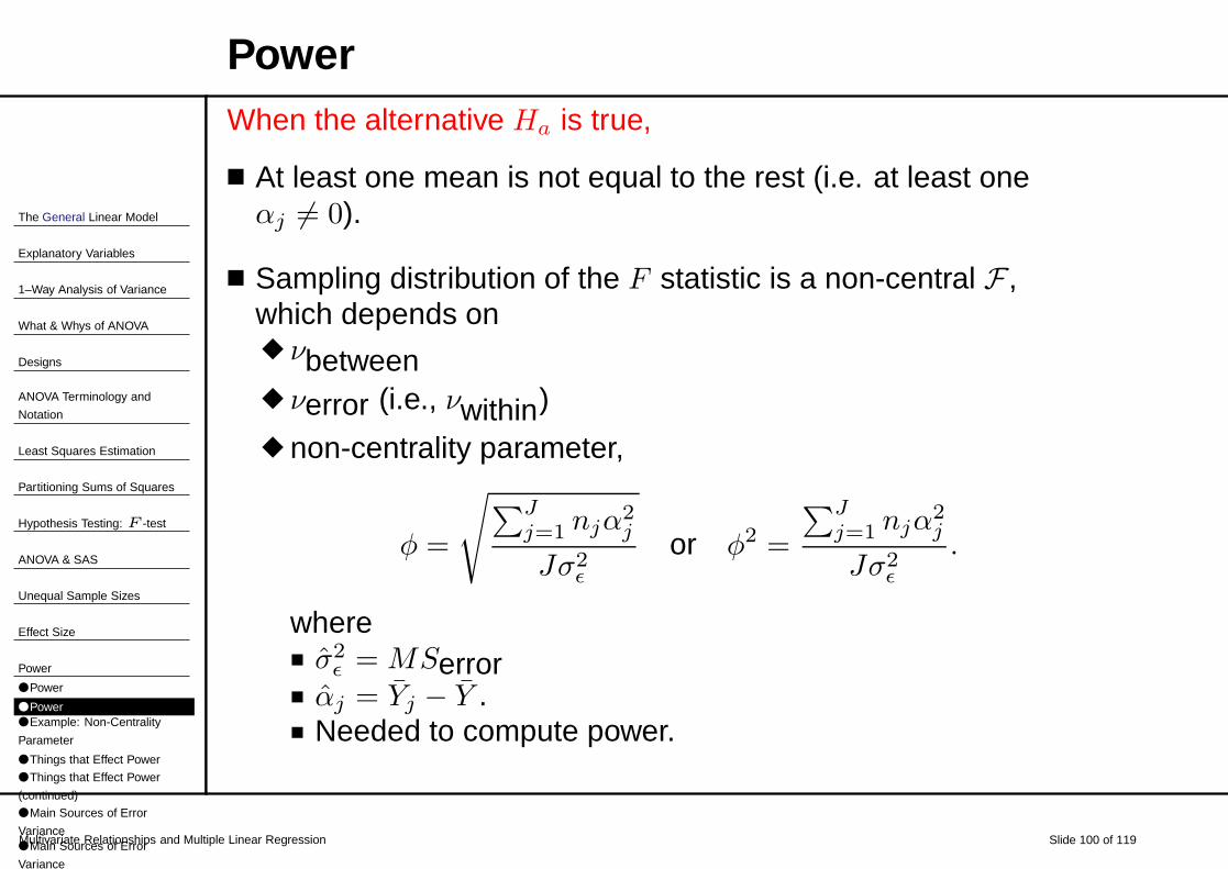
The General Linear Model
Explanatory Variables
1–Way Analysis of Variance
What & Whys of ANOVA
Designs
ANOVA Terminology and
Notation
Least Squares Estimation
Partitioning Sums of Squares
Hypothesis Testing: F -test
ANOVA & SAS
Unequal Sample Sizes
Effect Size
Power
● Power
● Power● Example: Non-Centrality
Parameter
● Things that Effect Power
● Things that Effect Power
(continued)
● Main Sources of Error
Variance● Main Sources of Error
Variance
Multivariate Relationships and Multiple Linear Regression Slide 100 of 119
PowerWhen the alternative Ha is true,
■ At least one mean is not equal to the rest (i.e. at least oneαj 6= 0).
■ Sampling distribution of the F statistic is a non-central F ,which depends on◆ νbetween◆ νerror (i.e., νwithin)
◆ non-centrality parameter,
φ =
√
∑Jj=1 njα2
j
Jσ2ǫ
or φ2 =
∑Jj=1 njα
2j
Jσ2ǫ
.
where■ σ2
ǫ = MSerror■ αj = Yj − Y .■ Needed to compute power.

The General Linear Model
Explanatory Variables
1–Way Analysis of Variance
What & Whys of ANOVA
Designs
ANOVA Terminology and
Notation
Least Squares Estimation
Partitioning Sums of Squares
Hypothesis Testing: F -test
ANOVA & SAS
Unequal Sample Sizes
Effect Size
Power
● Power
● Power● Example: Non-Centrality
Parameter
● Things that Effect Power
● Things that Effect Power
(continued)
● Main Sources of Error
Variance● Main Sources of Error
Variance
Multivariate Relationships and Multiple Linear Regression Slide 101 of 119
Example: Non-Centrality Parameter
Quality rating data (summary statistics on page 90, ANOVAsummary table on page 91):
■ Estimated treatment effects: αj = Yj − Y ,
αA = 5.0556−4.9216 = .1343, αC = 5.4167−4.9216 = .4954,
αU = 4.5091 − 4.9216 = −.4122
■ Non-centrality parameter:
φ2 =36(.1343)2 + 36(.4954)2 + 55(−.4122)2
3(.616)
=36(.01804) + 36(.2454) + 55(.1699)
1.848
=18.8283
1.848= 10.188

The General Linear Model
Explanatory Variables
1–Way Analysis of Variance
What & Whys of ANOVA
Designs
ANOVA Terminology and
Notation
Least Squares Estimation
Partitioning Sums of Squares
Hypothesis Testing: F -test
ANOVA & SAS
Unequal Sample Sizes
Effect Size
Power
● Power
● Power● Example: Non-Centrality
Parameter
● Things that Effect Power
● Things that Effect Power
(continued)
● Main Sources of Error
Variance● Main Sources of Error
Variance
Multivariate Relationships and Multiple Linear Regression Slide 102 of 119
Things that Effect Power
■ Prob(Type I Error) = α: ↑ α =⇒ Power ↑.
■ Within groups degrees of freedom, νw = νe:↑ νe =⇒ Power ↑.
■ Between groups, νb = J − 1 (least effect):↑ νb =⇒ Power ↑.
■ Cell sample size nj (related to νe):↑ nj =⇒ Power ↑.
■ Effect sizes, i.e., αj = µj − µ, or∑
j njαj :↑ αj =⇒ Power ↑.
■ Variance due to unsystematic sources, σ2ǫ : ↓ σ2
ǫ =⇒ Power ↑.

The General Linear Model
Explanatory Variables
1–Way Analysis of Variance
What & Whys of ANOVA
Designs
ANOVA Terminology and
Notation
Least Squares Estimation
Partitioning Sums of Squares
Hypothesis Testing: F -test
ANOVA & SAS
Unequal Sample Sizes
Effect Size
Power
● Power
● Power● Example: Non-Centrality
Parameter
● Things that Effect Power
● Things that Effect Power
(continued)
● Main Sources of Error
Variance● Main Sources of Error
Variance
Multivariate Relationships and Multiple Linear Regression Slide 103 of 119
Things that Effect Power (continued)
■ These things are inter-dependent (except for significancelevel).
■ To adjust and/or influence power during design stage,
◆ Sample size.◆ Error variance.
■ To compute power need to know:
αj , σ2ǫ , nj , and J.
■ Prospectively: make educated guesses.
■ Retrospectively: use data.

The General Linear Model
Explanatory Variables
1–Way Analysis of Variance
What & Whys of ANOVA
Designs
ANOVA Terminology and
Notation
Least Squares Estimation
Partitioning Sums of Squares
Hypothesis Testing: F -test
ANOVA & SAS
Unequal Sample Sizes
Effect Size
Power
● Power
● Power● Example: Non-Centrality
Parameter
● Things that Effect Power
● Things that Effect Power
(continued)
● Main Sources of Error
Variance● Main Sources of Error
Variance
Multivariate Relationships and Multiple Linear Regression Slide 104 of 119
Main Sources of Error Variance
■ Random variation in actual treatments (no experimentaltreatment is exactly the same for every subject),
e.g.,◆ calibration of equipment
◆ environmental factors (noise, humidity, temperature,illumination, etc),
◆ training & experience of experimenters.
■ Unanalyzed control factors or “nuisance” factors: Add themto analysis so not confounded with treatment.

The General Linear Model
Explanatory Variables
1–Way Analysis of Variance
What & Whys of ANOVA
Designs
ANOVA Terminology and
Notation
Least Squares Estimation
Partitioning Sums of Squares
Hypothesis Testing: F -test
ANOVA & SAS
Unequal Sample Sizes
Effect Size
Power
● Power
● Power● Example: Non-Centrality
Parameter
● Things that Effect Power
● Things that Effect Power
(continued)
● Main Sources of Error
Variance● Main Sources of Error
Variance
Multivariate Relationships and Multiple Linear Regression Slide 105 of 119
Main Sources of Error Variance
■ Individual differences or subject variability:
◆ Select subjects who are similar with respect to importantand relevant characteristics.
◆ Type of “matching”
◆ Repeated measures
◆ Analysis of covariance.

The General Linear Model
Explanatory Variables
1–Way Analysis of Variance
What & Whys of ANOVA
Designs
ANOVA Terminology and
Notation
Least Squares Estimation
Partitioning Sums of Squares
Hypothesis Testing: F -test
ANOVA & SAS
Unequal Sample Sizes
Effect Size
Power
● Power
● Power● Example: Non-Centrality
Parameter
● Things that Effect Power
● Things that Effect Power
(continued)
● Main Sources of Error
Variance● Main Sources of Error
Variance
Multivariate Relationships and Multiple Linear Regression Slide 106 of 119
Computing Power (or Sample Size)
SAS/ANALYST — only equal sample sizes
■ Solutions> Analysis > Analyst > Statistics > Sample size >One-way ANOVA.
■ In the window that opens up, you will need to enter (made upnumbers):
Calculate power The other option is sample size# of treatments 3 J
CSS of Means .38375 This equals∑
j(µj − µ)2
Standard Deviation .49551 This is square root of MSerror
Alpha .05 Significance levelN per group From 5
To 20By 1
■ Click “OK”.

The General Linear Model
Explanatory Variables
1–Way Analysis of Variance
What & Whys of ANOVA
Designs
ANOVA Terminology and
Notation
Least Squares Estimation
Partitioning Sums of Squares
Hypothesis Testing: F -test
ANOVA & SAS
Unequal Sample Sizes
Effect Size
Power
● Power
● Power● Example: Non-Centrality
Parameter
● Things that Effect Power
● Things that Effect Power
(continued)
● Main Sources of Error
Variance● Main Sources of Error
Variance
Multivariate Relationships and Multiple Linear Regression Slide 107 of 119
Sample Size TableOne-Way ANOVA
# Treatments = 3 CSS of Means = .38375
Standard Deviation = .49551 Alpha = 0.05
N per
Group Power
5 0.588
6 0.696
7 0.781
8 0.845
9 0.893
10 0.927
11 0.950
12 0.967
13 0.978
14 0.986
15 >.99
16 >.99
17 >.99

The General Linear Model
Explanatory Variables
1–Way Analysis of Variance
What & Whys of ANOVA
Designs
ANOVA Terminology and
Notation
Least Squares Estimation
Partitioning Sums of Squares
Hypothesis Testing: F -test
ANOVA & SAS
Unequal Sample Sizes
Effect Size
Power
● Power
● Power● Example: Non-Centrality
Parameter
● Things that Effect Power
● Things that Effect Power
(continued)
● Main Sources of Error
Variance● Main Sources of Error
Variance
Multivariate Relationships and Multiple Linear Regression Slide 108 of 119
Power Plot
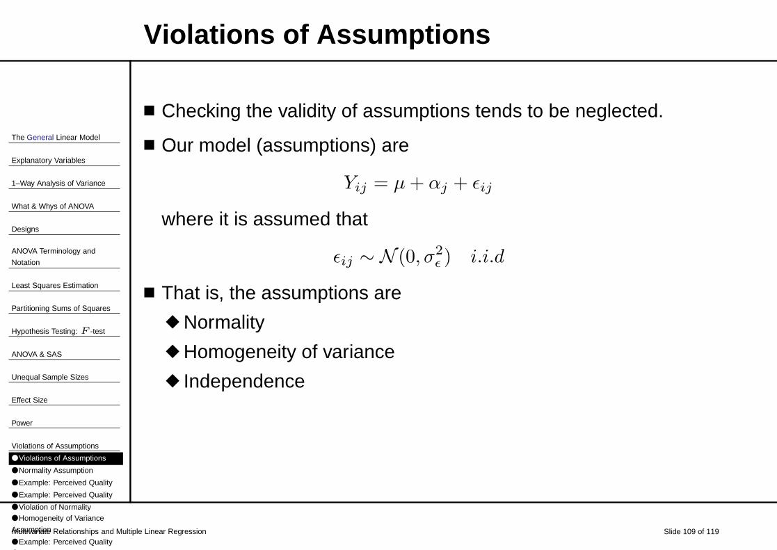
The General Linear Model
Explanatory Variables
1–Way Analysis of Variance
What & Whys of ANOVA
Designs
ANOVA Terminology and
Notation
Least Squares Estimation
Partitioning Sums of Squares
Hypothesis Testing: F -test
ANOVA & SAS
Unequal Sample Sizes
Effect Size
Power
Violations of Assumptions
● Violations of Assumptions
● Normality Assumption
● Example: Perceived Quality
● Example: Perceived Quality
● Violation of Normality
● Homogeneity of Variance
Assumption
● Example: Perceived Quality
● Effect of Heterogeneous
Multivariate Relationships and Multiple Linear Regression Slide 109 of 119
Violations of Assumptions
■ Checking the validity of assumptions tends to be neglected.
■ Our model (assumptions) are
Yij = µ + αj + ǫij
where it is assumed that
ǫij ∼ N (0, σ2ǫ ) i.i.d
■ That is, the assumptions are◆ Normality
◆ Homogeneity of variance◆ Independence

The General Linear Model
Explanatory Variables
1–Way Analysis of Variance
What & Whys of ANOVA
Designs
ANOVA Terminology and
Notation
Least Squares Estimation
Partitioning Sums of Squares
Hypothesis Testing: F -test
ANOVA & SAS
Unequal Sample Sizes
Effect Size
Power
Violations of Assumptions
● Violations of Assumptions
● Normality Assumption
● Example: Perceived Quality
● Example: Perceived Quality
● Violation of Normality
● Homogeneity of Variance
Assumption
● Example: Perceived Quality
● Effect of Heterogeneous
Multivariate Relationships and Multiple Linear Regression Slide 110 of 119
Normality Assumption
■ The Assumption: Errors (and hence Yij) are normallydistributed.
■ Detection of non-normality:
◆ Histograms, box-plots, stem-n-leaf displays of ǫij (or Yij).
◆ Normal probability plot of ǫij = Yij − Yj .
◆ Statistical tests of normality (Kolmogorov D, Wilk-Shaprio)

The General Linear Model
Explanatory Variables
1–Way Analysis of Variance
What & Whys of ANOVA
Designs
ANOVA Terminology and
Notation
Least Squares Estimation
Partitioning Sums of Squares
Hypothesis Testing: F -test
ANOVA & SAS
Unequal Sample Sizes
Effect Size
Power
Violations of Assumptions
● Violations of Assumptions
● Normality Assumption
● Example: Perceived Quality
● Example: Perceived Quality
● Violation of Normality
● Homogeneity of Variance
Assumption
● Example: Perceived Quality
● Effect of Heterogeneous
Multivariate Relationships and Multiple Linear Regression Slide 111 of 119
Example: Perceived Quality

The General Linear Model
Explanatory Variables
1–Way Analysis of Variance
What & Whys of ANOVA
Designs
ANOVA Terminology and
Notation
Least Squares Estimation
Partitioning Sums of Squares
Hypothesis Testing: F -test
ANOVA & SAS
Unequal Sample Sizes
Effect Size
Power
Violations of Assumptions
● Violations of Assumptions
● Normality Assumption
● Example: Perceived Quality
● Example: Perceived Quality
● Violation of Normality
● Homogeneity of Variance
Assumption
● Example: Perceived Quality
● Effect of Heterogeneous
Multivariate Relationships and Multiple Linear Regression Slide 112 of 119
Example: Perceived Quality

The General Linear Model
Explanatory Variables
1–Way Analysis of Variance
What & Whys of ANOVA
Designs
ANOVA Terminology and
Notation
Least Squares Estimation
Partitioning Sums of Squares
Hypothesis Testing: F -test
ANOVA & SAS
Unequal Sample Sizes
Effect Size
Power
Violations of Assumptions
● Violations of Assumptions
● Normality Assumption
● Example: Perceived Quality
● Example: Perceived Quality
● Violation of Normality
● Homogeneity of Variance
Assumption
● Example: Perceived Quality
● Effect of Heterogeneous
Multivariate Relationships and Multiple Linear Regression Slide 113 of 119
Violation of Normality
■ Non-normality tends to have negligible effects on theprobability of errors (i.e, α and β), except
1. When nj ’s are small.
2. When distributions are highly skewed. e.g.,◆ Binomial variable with tiny π.◆ Test scores with a “ceiling” or “floor”.
■ Remedies:1. Get larger samples.
2. Use more appropriate statistical procedure. e.g.,non-parametric test, generalized linear model.

The General Linear Model
Explanatory Variables
1–Way Analysis of Variance
What & Whys of ANOVA
Designs
ANOVA Terminology and
Notation
Least Squares Estimation
Partitioning Sums of Squares
Hypothesis Testing: F -test
ANOVA & SAS
Unequal Sample Sizes
Effect Size
Power
Violations of Assumptions
● Violations of Assumptions
● Normality Assumption
● Example: Perceived Quality
● Example: Perceived Quality
● Violation of Normality
● Homogeneity of Variance
Assumption
● Example: Perceived Quality
● Effect of Heterogeneous
Multivariate Relationships and Multiple Linear Regression Slide 114 of 119
Homogeneity of Variance Assumption
■ The Assumption: σ21 = σ2
2 = . . . = σ2J
■ Detection of heterogeneous variances
◆ If you have large samples from normal populations,statistical test of homogeneity of variance (e.g., Bartlett,Cochran, Schaffé, and others’ test).
◆ Use what you know about the data. e.g., If the dependentor response variable is a count or frequency — beware.
◆ Graphical display: plot σj = sj versus Xj .
■ Out data. . .

The General Linear Model
Explanatory Variables
1–Way Analysis of Variance
What & Whys of ANOVA
Designs
ANOVA Terminology and
Notation
Least Squares Estimation
Partitioning Sums of Squares
Hypothesis Testing: F -test
ANOVA & SAS
Unequal Sample Sizes
Effect Size
Power
Violations of Assumptions
● Violations of Assumptions
● Normality Assumption
● Example: Perceived Quality
● Example: Perceived Quality
● Violation of Normality
● Homogeneity of Variance
Assumption
● Example: Perceived Quality
● Effect of Heterogeneous
Multivariate Relationships and Multiple Linear Regression Slide 115 of 119
Example: Perceived Quality
Level nj Yj sj s2j
Affirm 36 5.056 0.826 0.683Control 36 5.417 0.874 0.764
Undermine 55 4.509 0.690 0.477
From SAS/ANLAYST: TestTest df SS MS Statistic p-value
Levene’s testgroup 2 1.8389 0.9194 F = 1.68 .19Error 124 67.6690 0.5457
Brown and Forsythe’s Testgroup 2 0.3728 0.1864 F = 0.48 .62Error 124 47.7217 0.3849
Bartlett’s Testgroup 2 χ2 = 2.67 0.26

The General Linear Model
Explanatory Variables
1–Way Analysis of Variance
What & Whys of ANOVA
Designs
ANOVA Terminology and
Notation
Least Squares Estimation
Partitioning Sums of Squares
Hypothesis Testing: F -test
ANOVA & SAS
Unequal Sample Sizes
Effect Size
Power
Violations of Assumptions
● Violations of Assumptions
● Normality Assumption
● Example: Perceived Quality
● Example: Perceived Quality
● Violation of Normality
● Homogeneity of Variance
Assumption
● Example: Perceived Quality
● Effect of Heterogeneous
Multivariate Relationships and Multiple Linear Regression Slide 116 of 119
Effect of Heterogeneous Variance
■ Little (negligible) when nj = n (i.e., a balanced design).
■ Systematic effects
◆ When n1 > n2 and s21 > s2
2, the test is conservative; theactual α is smaller than desired.
◆ When n1 < n2 and s21 > s2
2, the test is liberal; the actual αlevel is larger than desired.
■ Remedies: Use same ones as recommended for twoindependent groups t-test.

The General Linear Model
Explanatory Variables
1–Way Analysis of Variance
What & Whys of ANOVA
Designs
ANOVA Terminology and
Notation
Least Squares Estimation
Partitioning Sums of Squares
Hypothesis Testing: F -test
ANOVA & SAS
Unequal Sample Sizes
Effect Size
Power
Violations of Assumptions
● Violations of Assumptions
● Normality Assumption
● Example: Perceived Quality
● Example: Perceived Quality
● Violation of Normality
● Homogeneity of Variance
Assumption
● Example: Perceived Quality
● Effect of Heterogeneous
Multivariate Relationships and Multiple Linear Regression Slide 117 of 119
The Independence Assumption
■ The assumption: Yij are independent within and betweengroups.
■ Detection of violation:
◆ Hard; rely on what you know about the experimentalprocedures and data collection.
◆ Compute intra-class correlation.
■ Our data on quality ratings, rintra = .32 (not significant).

The General Linear Model
Explanatory Variables
1–Way Analysis of Variance
What & Whys of ANOVA
Designs
ANOVA Terminology and
Notation
Least Squares Estimation
Partitioning Sums of Squares
Hypothesis Testing: F -test
ANOVA & SAS
Unequal Sample Sizes
Effect Size
Power
Violations of Assumptions
● Violations of Assumptions
● Normality Assumption
● Example: Perceived Quality
● Example: Perceived Quality
● Violation of Normality
● Homogeneity of Variance
Assumption
● Example: Perceived Quality
● Effect of Heterogeneous
Multivariate Relationships and Multiple Linear Regression Slide 118 of 119
SAS/Intraclass Correlation
proc mixed data=quality noclprint covtest method=REML;class group;model qual = / solution;random int /subject=group;title ’Random effects ANOVA/ random intercept HLM (nullmodel)’;run;
Edited SAS output:
Covariance Parameter EstimatesCov Parm Subject Estimate
Intercept group 0.1963Residual 0.6159
rintra =.1963
.6159= .3187

The General Linear Model
Explanatory Variables
1–Way Analysis of Variance
What & Whys of ANOVA
Designs
ANOVA Terminology and
Notation
Least Squares Estimation
Partitioning Sums of Squares
Hypothesis Testing: F -test
ANOVA & SAS
Unequal Sample Sizes
Effect Size
Power
Violations of Assumptions
● Violations of Assumptions
● Normality Assumption
● Example: Perceived Quality
● Example: Perceived Quality
● Violation of Normality
● Homogeneity of Variance
Assumption
● Example: Perceived Quality
● Effect of Heterogeneous
Multivariate Relationships and Multiple Linear Regression Slide 119 of 119
Effect of Violating Independence
■ Effect of Dependence (serious problem).◆ Effects significance level and power of the F test.◆ When observations are dependent, the actual/ true
probability of a Type I error is likely to be larger than thestated one, i.e, If there is a positive association betweenresponses, true α > desired α.
■ Remedies:◆ If appropriate, use another model.◆ Re-do the study/experiment using improved procedures.