General Dynamical Equations of Motion for Elastic Body Systems

JOURNAL OF GUIDANCE, CONTROL, AND DYNAMICSVol. 15, No. 6, November-December 1992

General Dynamical Equations of Motionfor Elastic Body Systems

Shui-Lin Weng* and Donald T. Greenwood!University of Michigan, Ann Arbor, Michigan 48109

A modeling technique capable of determining the time response of a single body (rigid or flexible) that is, ingeneral, undergoing large elastic deformations, coupled with large, nonsteady translational and rotationalmotions, is presented. The derivations of the governing equations of motion are based on Lagrange's form ofd'Alembert's principle. The general dynamical equations of motion are expressed in terms of stress and straintensors, kinematic variables, the velocity and angular velocity coefficients, and generalized forces. The formu-lation of these equations is discussed in detail. Numerical simulations that involve finite elastic deformationscoupled with large, nonsteady rotational motions are presented for a beam attached to a rotating base. Effectssuch as centrifugal stiffening and softening, membrane strain effect, and vibrations induced by Coriolis forcesare accommodated. The effects of rotary inertia as well as shear deformation are also included in the equationsof motion. Although discussions here are restricted to a single body, the formulation allows the capability of ageneral dynamical formalism for handling multibody (rigid or flexible) dynamics.

I. Introduction

H OOKER and Margulies1 as well as Roberson and Witten-burg2 wrote early papers in the mid-1960s that dealt

primarily with spacecraft dynamics. The methodologies theypresented were applicable only to systems of rigid bodies withsimple joints in a restricted configuration. Later, a number ofstudies based on these methods were published.3'4 A typicalmodern spacecraft consists of structural subsystems, some es-sentially rigid and others extremely flexible, frequently inter-connected in a time-varying manner. Formulation dealing withthis category of spacecraft is a procedure that employs discretecoordinates to describe the unrestricted motions of thosestructural subsystems idealized as rigid bodies, in combinationwith distributed or modal coordinates to describe the time-varying deformations of those structural subsystems idealizedas flexible elastic appendages.5'6 Advances also have beenmade concerning the coupling effects between gross transla-tional or rotational motion and the elastic deformation ofelastic bodies.7'11

Repeated numerical simulations are needed to establish asatisfactory design for the prototype of a spacecraft. In aneffort to facilitate the simulations of multiple interconnectedbodies, analysts have come to rely more and more on generalmultibody dynamics formalisms. A dynamical system may betranslating or spinning in whole or in part and may be expectedto undergo large changes in inertial position and orientation.It has become necessary to devise methods of dynamic analysisthat combine the generalities of nonlinearities and large mo-tions with the computational efficiency afforded by the use ofmodal coordinates in describing the vehicle deformations.

Mathematical modeling tools are used to analyze the prob-lems and to derive the dynamical equations of motion for amultibody system. Comparative studies12 suggest that Kane'smethod13'14 or some related generalization of Lagrange's formof d'Alembert's principle15 most closely combines the two com-putational advantages: 1) the nonworking constraint forces

Received Nov. 15, 1990; revision received Nov. 15, 1991; acceptedfor publication Nov. 27, 1991. Copyright © 1992 by the AmericanInstitute of Aeronautics and Astronautics, Inc. All rights reserved.

* Graduate Research Assistant, Department of Aerospace Engineer-ing; currently, Researcher, Center for Aviation and Space Technol-ogy, ITRI, Hsinchu, Taiwan. Member AIAA.

fProfessor, Department of Aerospace Engineering. Associate Fel-low AIAA.

and torques do not appear and 2) the resulting equation set isof minimum dimension.

A modeling technique capable of determining the time re-sponse of a rigid or flexible body that is, in general, under-going large elastic deformations, coupled with large, non-steady translational and rotational motions, is considered. Thederivations of the governing equations of motion are based onLagrange's form of d'Alembert's principle. The general dy-namical equations of motion are expressed in terms of stressand strain tensors, kinematic variables, the velocity and angu-lar velocity coefficients, and generalized forces. These equa-tions can be derived systematically.

It is well known that when flexible structural elements areattached to a rotating base, the apparent stiffness of the struc-tural elements varies with the magnitude of the inertial angularvelocity of the spinning base. Also, in linear structural theory,the transverse vibration of a beam is calculated without consid-ering axial forces. But in some cases, e.g., in rapidly rotatingturbine or helicopter blades, it is not possible to ignore theeffect of axial forces on the bending vibration of blades. Whenthe beamlike blade is spinning, so-called centrifugal stiffeningeffects that are due to the presence of axial (centrifugal) forcescome into play. Coupling betwen centrifugal forces and bend-ing moments makes a rapidly spinning beam stiffer than ispredicted by linear theory. In the light of this situation, it isimportant that a multibody formulation correctly reflects mo-tion-induced stiffness.

To resolve the difficulties, a single generalized formalism,the general dynamical equations of motion, is introduced. It isdistinguished from a method using the shortening effect16'18

explicitly in that here the centrifugal stiffening terms enter thefinal equations through the potential energy rather thanthrough the kinetic energy. Also, we investigate the mecha-nism of motion-induced stiffness variations in various types ofelastodynamic structures undergoing large overall motions.Effects such as centrifugal stiffening and softening, membranestrain effect, and vibrations induced by Coriolis forces areaccommodated. The effects of rotary inertia as well as sheardeformation are also included in the equations of motion.

In Sec. II, we include the finite displacement theory of elas-ticity, the principle of virtual work, and the preliminaries tothe actual dynamical problem for the purpose of complete-ness. In Sec. Ill, a generalized formalism to analyze the dy-namical system, the general dynamical equations of motionbased on Lagrange's form of d'Alembert's principle, is devel-oped. In Sec. IV, an analysis of a single flexible beam is pre-

1434

WENG AND GREENWOOD: GENERAL DYNAMICAL EQUATIONS OF MOTION 1435

sented to illustrate the formulating procedures of the generaldynamical equations of motion. Section V applies the flexiblebeam theory of Sec. IV to several problems. Section VI pre-sents the conclusions.

II. Modeling of Flexible BodiesIn this investigation, we assume that a rigid or deformable

body may experience large translational or rotational displace-ments relative to an inertial coordinate system. Although abody-axis system that is rigidly attached to a point on the bodyis commonly employed as a reference for rigid components,there are many arrangements for the body axes of flexiblecomponents.19'20 The origin of this reference frame does nothave to be rigidly attached to a point on the deformable body,but frequently it is so chosen. We will attach the body axes toa small rigid volume element at one end of the beam.

Analysis of StrainIn the present section, we shall treat the finite displacement

theory of elasticity in rectangular Cartesian coordinates andemploy the Lagrangian approach, in which the coordinatesdefining a point of the body before deformation are employedfor locating the point during the subsequent deformation.

Let a rectangular Cartesian coordinate system xlx2x3 beassigned to each body, and let the relative position vector ofan arbitrary point P(0) of the body before deformation berepresented by

as shown in Fig. 1, where the superscript (0) means that thequantity refers to the state before deformation. The base vec-tors in this coordinate system are given by

(2)

where the notation ( ) > M denotes differentiation with respect toJCM. The base vectors are unit vectors in the direction of thecoordinate axes and are mutually orthogonal.

The body is now assumed to be deformed into a strainedconfiguration. The points P(0), Q(0\ R<®, S(0), and T^ moveto new positions denoted by P, Q, R, S, and T, respectively,and the infinitesimal rectangular parallelepiped is deformedinto a parallelepiped that, in general, is no longer rectangular.Let us denote the position vector of the point P relative tothe body frame by

r = r(xl, x2, x3) (3)

where (xl,x2,x3) are actually the Cartesian coordinates ofP(0). Introduce the lattice vectors defined by

8rG * = l , 2 , 3 ) (4)

T(O)

Fig. 2 Geometry of body axes and inertial axes.

In general, the lattice vectors are neither unit vectors nor arethey mutually orthogonal.

Next, let us express the position vector of the point P as

r = r<°> + d (5)

where d is the elastic displacement vector expressed in thej-frame. From Eqs. (4) and (5), we have

(6)

where 6* is the Kronecker symbol. The summation conven-tion will be employed hereafter. Therefore a Greek letter indexjit, f, x, or K that appears twice in the same term indicates asummation over (1, 2, 3). Consequently, Green's strain tensorcan be calculated in terms of the displacement components asfollows:

(7)

Analysis of Stress and Stress-Strain RelationsThe force equation for the equilibrium of the deformed

parallelepiped is given by21

= 0 (8)

where a^ is the second Piola-Kirchhoff stress vector acting onthe jLtth face of the deformed parallelepiped, and F is the bodyforce acting in this parallelepiped. We note that aM is definedper unit area, and F is defined per unit volume, both withrespect to the undeformed state.

Assume that the material is isotropic. The stress-strain rela-tion is21

Ev(9)

where Young's modulus E, Poisson's ratio v, and the shearmodulus G are related by E = 2(1 + v)G.

Dynamics of an Elastic BodyLet a rectangular Cartesian coordinate system Xl X 2X3 be

fixed in inertial space, and let the corresponding unit vectorsystem be ii /21*3, as shown in Fig. 2. The origin of the body-axis system xlx2x3 is located at a position rG relative to theorigin of the inertial frame. Then the inertial position vector r(see Fig. 2) of a representative point P of the elastic body is

r = rG + r<°> + d (10)

Fig. 1 Geometry of an infinitesimal parallelepiped.

where we recall that r<®(xl, x2, x3) is its position relative to thebody frame before deformation, and d is its elastic deforma-tion vector relative to the body frame. The vector rG is ex-

1436 WENG AND GREENWOOD: GENERAL DYNAMICAL EQUATIONS OF MOTION

Fig. 3 Geometry of a rigid body.

pressed in terms of its inertial components, but r(0) and d areexpressed iny-frame components; that is,

and

From Eq. (10), we obtain

where the absolute angular velocity of they -frame is

(13)

and where (dd/dt)r is the rate change of d as viewed from thisrotating frame in which the j^ unit vectors are constant.

The dynamical equations of motion are obtained by usingd'Alembert's principle in its Lagrangian form involving vir-tual work. Here we lump the inertia force -p(d2r/dt2) withthe body force F, each per unit volume. We consider an elas-tic body that is subject to body forces F(xl,x2

9x3,t) dis-tributed throughout the body, surface forces B(xl

9x29x3

9t)applied on the surface Si, and specified surface displacementsr(xl, Jc2, x3, t) on the surface S2. The virtual work expressionfor the dynamical problem is

d2A-p—- - 6 r d Kv\ dt2)

B - 5r dS = 0 (14)

The first integral represents the first variation of the storedelastic energy, whereas the second integral represents the vir-tual work of the body forces and inertia forces, and the thirdintegral represents the virtual work of the surface forces actingon Si. As the motion of the surface S2 is prescribed, it does notenter into the virtual work expression. The virtual displace-ment dr is given by

dr = 5rG + WyM + 69 x (r<°> + d) (15)

where 60 is the virtual rotation of the body axes; i.e., thej- frame.

III. General Dynamical Equations of MotionLet us begin with the matrix equation relating the unit vec-

tors of the body-axis j -frame and the inertial /-frame, whereA is an orthogonal matrix:

Using Eq. (6), we see that Lx and / r are related by

where Z is the nonorthogonal matrix:

l+</22 d?2

-",3

(18)

Genera! Case: Elastic BodyWe can write Eq. (14) in the following form and see each

term more explicitly:

d2r*V

P dt2

(11) ^e can a*so rewrite Eq. (15) as follows:

(19)

(20)

Let {a£ ) be the L -frame skewed components and let {o f } bethe /-frame components of the same stress vector a*. Then

Now we revert to the notation {a£ ) = { a ^ } and write Eqs. (19)and (20) in matrix form as

( [ A ] T { F } ) T ( d r } d V + ( [ A ] T [ B } ) T l d r } d Ss,

and= idrG] + [A]T[5d] +

(22)

(23)

Here [60] is a 3 x 3 skew-symmetric matrix representing thevector cross-product. In addition to the preceding two expres-sions, we still need to know [6r > / x ) . Note that {rG} is not afunction of body axis variables; we obtain

(24)

Suppose we have n generalized coordinates, and those corre-sponding to elastic displacements are associated with assumeddeflection forms. Then, in terms of x and q, we have

= (d(x9q)} (25)

(17) Fig. 4 Rotating cantilever beam.


where x represents the spatial variables (x\ x2, x3). The abso-lute velocity of the point G is

(v } = \r ] = yJL<r i A . + J L r r j (26)

Next, let us define the velocity coefficient {yf} due to QJ as

G = — d

where /-frame components are chosen. The virtual displace-ment [drc } can be expressed as

^ a (yf (28)

The virtual displacement [dd] can be derived using a similarprocedure. The velocity {d} due to #/ of the generic point Pis a relative velocity, and we find that

d}=p^ ( d ] q j (29)

The relative velocity coefficient { yj } due to QJ is

iyj} = ̂ r [d] = /- [d] (30)d<lj d<lj

where the components are expressed in they -frame. So thevirtual displacement [dd] can be expressed as

( « r f ) = £ ^- Wbq = t [yj}dqj (31)y = i d<?y j=\

and the spatial derivative of the virtual displacement { dd } canalso be expressed as

(32)

To obtain the virtual work due to inertial moments, we firstdefine the angular velocity coefficient ( /37) as follows:

(33)

where {oj) is the absolute angular velocity of they -axis system.Then we can express a small virtual rotation {50) in the form

(34)

Now we are ready to consider the first integral of Eq. (22).When we substitute Eq. (23) into this integral, and use j-framecomponents, we obtain

( [ A ] T { F } ) T [ 5 r } d V = l F ] T ( [ A ] i d r G }/• 1 I I ¥/• \

V (35)

The terms on the right-hand side of Eq. (35) represent thevirtual work due to the resultant applied forces. By intro-ducing the virtual displacements of Eqs. (28) and (31), andthe virtual rotation of Eq. (34), into the right-hand side ofEq. (35), we obtain

Bv

where the superscript B denotes an applied body force. Also,

and

fc r5) _ f cr \ fl&\[ o j — [ o j vyo/

By a similar procedure, we obtain the second integral ofEq. (22) in the form

j (39)

where the superscript S denotes an applied external surfaceforce and

{ 5 S } = [B} (40)

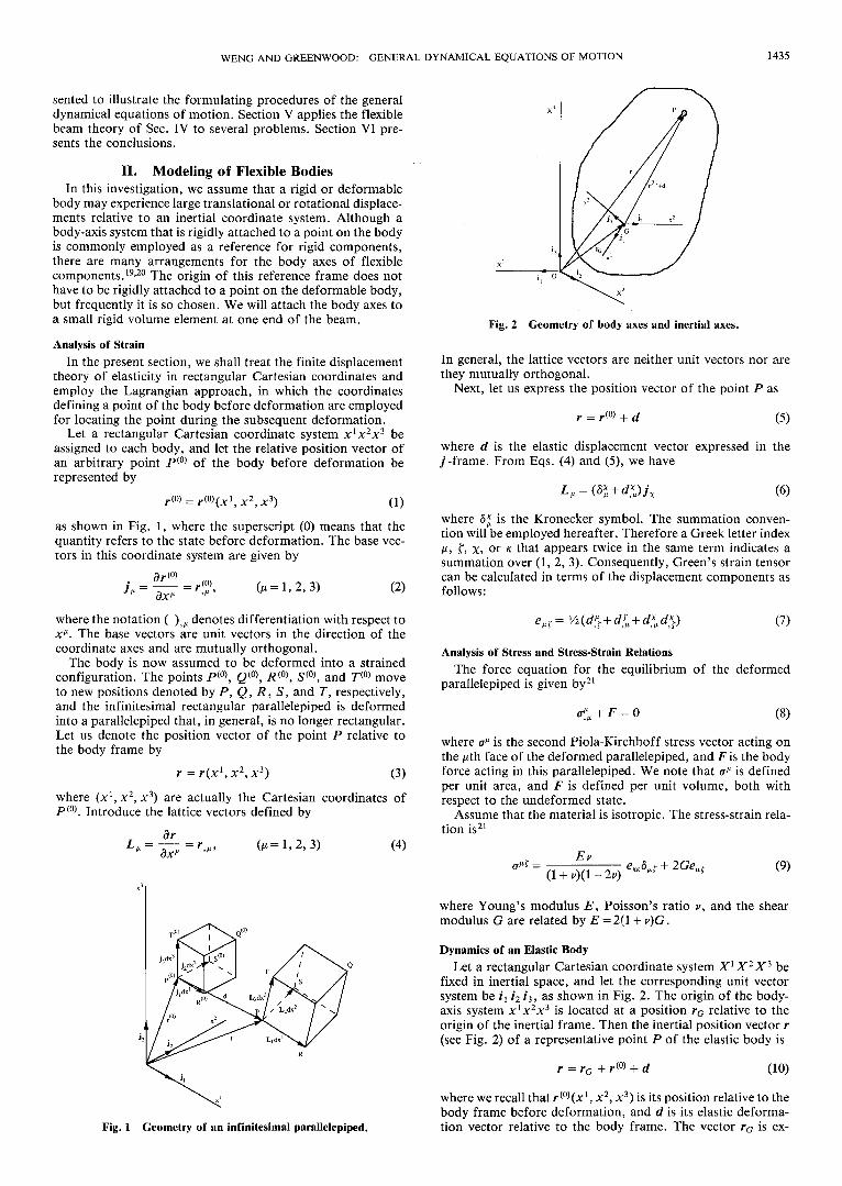
Next, let us consider the third integral of Eq. (22) where weneed to compute { r } . We know from Eq. (10) that r can beexpressed in matrix form as

Now [ A ] , ( r G ) , and {d} all vary with time, but (r (0)) doesnot. So, taking the derivative of Eq. (41) twice, with respect totime t, we obtain

[A]T[5>]2lr«»}

Fig. 5 Flexible beam cantilevered at the rim of a rigid wheel.

(42)

where we note that [^4] = - [<£] [A ] = [w] T[A ] .Substitute Eqs. (42) and (23) into the third integral of Eq.

(22), and then substitute the virtual displacements of Eqs. (28)and (31) and the virtual rotation of Eq. (34) into the formerresult, obtaining

j (43)

where the asterisk denotes an inertial force. Using j -framecomponents,

(44)

Finally, we shall consider the fourth integral of Eq. (22),which involves the stress tensor. If we substitute Eq. (24) intothe fourth integral of Eq. (22), and use the derivative of virtual


0.005

0.000

>-0.005

3-0.010

-0.015

-0.0200.0 5.0 10.0 15.0 20.0 25.0 30.0

t (sec)

Fig. 6 The x displacement u vs time t.

o.i

0.0

-0. 1

IT -0.2

f -0.3

-0.4

-0.5

-0.60.0 5.0 10.0 15.0 20.0 25.0 30.0

t (sec)

Fig. 7 The y displacement v vs time t.

displacement of Eq. (32) and of virtual rotation of Eq. (34), weobtain, after switching toy-frame components,

dV

7=UJJ V

where the superscript E denotes an elastic force and

= -[Z]Ti^}

(45)

(46)

Note that no elastic energy is stored due to a rigid body dis-placement, so only elastic displacements are considered here.

Next, in accordance with d'Alembert's principle, we cansum the virtual work of the applied and inertial generalizedforces to obtain

(47)

where bq conforms to any constraints.Let Qj, Qf, and Qf be the generalized external applied

forces, the generalized inertia forces, and the generalized elas-tic forces, respectively, and we obtain the following expres-sions:

Qj =

Qf =

Hence, we see that d'Alembert's principle leads once again to

£(Q; + G; + e/)««/ = 0 (48)y=i

More explicitly, however, with the aid of Eqs. (36), (39), (43),and (45) we obtain

Next, let us make the further assumption that the variousq are independent. Then each coefficient of dqj vanishes inEq. (48) and we obtain

QJ + Qf + Qf = o,or in greater detail,

(50)

dVJdqj = 0 (49)

C/ = l ,2 , . . . ,n ) (51)Equation (51) is the matrix form of the general dynamical

equations of motion for a system that is not subject to holo-nomic and nonholonomic constraints on the generalized coor-dinates. Now, let us take a closer look at the problems ofrepresenting the dynamical equations of constrained systems.

Constrained SystemsConsider a system whose configuration is given by n gener-

alized coordinates q\,q2>--,qn- Suppose there are m inde-pendent constraints of the form

(52)

where these expressions are not integrable for the case of non-holonomic constraints. If the constraints are actually holo-nomic and of the form

(53)

then, upon differentiation with respect to time, they have theform of Eq. (52) but are integrable. In either case, let usintroduce a set of (n - m) independent velocity parameters wy ,known as generalized speeds,14 which are consistent with theconstraints and are related to q by the equations

(54)

where u may represent true velocities or quasivelocities; i.e.,there is no integrability requirement on Eq. (52). If Eqs. (52)and (54) are solved for q in terms of u , one obtains

4f /="xfMtf>OH; + */fte,0, (i = 1,2,. . . , /i) (55)


For this constrained system, one can use Eq. (55) to elimi-nate q in favor of a set of (n -m) independent u as velocityparameters. Then Eq. (51) still applies if one defines the veloc-ity coefficients and angular velocity coefficients with respect tothese new velocity parameters, that is,

Thus, we obtain (n -m) dynamical equations

C/ = l , 2 , . . . , w - / n ) (56)

where Q represents generalized forces associated with u andwhere

yj] = [A](yf] (57)

Special Case: Rigid BodyNow, consider the special case of a rigid body motion. The

origin G is the reference point and we assume that this point isfixed in the body (see Fig. 3). The mass of the body is m , andits center mass position relative to G is pc. Also, we know that

p d V = m and (58)

After some algebraic manipulations, the general dynamicalequation of motion (51) becomes,22 in vector form,

(j = l,2,. . . , / i ) (59)

where there are n independent generalized coordinates. Noticethat the inertia dyadic / is taken about its reference point at G .

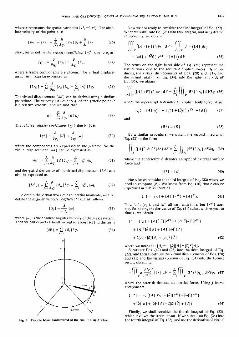
IV. Analysis of Flexible BeamsWhen flexible structural elements are attached to a rotating

base, as shown in Figs. 4 and 5, the apparent stiffness of thestructural elements varies with the magnitude of the inertialangular velocity of the spinning base. For some base-elementattachment configurations as in Fig. 4, the stiffness of theelements increases with base angular speed,23 whereas for oth-ers, such as Fig. 5, the stiffness decreases.24 In this section weanalyze the deflection of a flexible beam with large overallmotions, which performs a prescribed planar rotational mo-tion around the i'3-axis (or yr axis), by using the general dynam-ical equations of motion.

Now let us derive the differential equations of motion forthis rotating beam (see Fig. 4), whose motion is confined to theX- Yplane. We choose xyz as body axes and the origin G as thereference point for the beam. Generalized coordinates QJ(j = 1,2, . . . ,n) will be used to represent the configuration ofthe rotating beam at any time /. The velocity of the referencepoint G is zero. This leads to the velocity coefficients (yf ]being equal to zero. The angular velocity of they-frame isprescribed as a function of time, so the corresponding angularvelocity coefficients [fy] all vanish. Also, we assume thatthere are no applied forces, so the generalized external appliedforces QJ are zero. But the velocity coefficients (7^) resultingfrom elastic deformations and their spatial derivatives arenonzero.

Next, let us make the following assumptions. First, by thechoice of axes and from the definition of the central line as theline of centroids of the cross sections, we have

(60)y dy dz = z dy dz = yz dy dz = 0

where A is the area of the cross section. Second, the centroidaldisplacement vector {D} = {uv w}Tis a function of x and qonly, and we set w =0. Third, we assume that the stress com-ponents ayy, azz, axz, and ayz may be neglected in comparisonwith the other stress components, and then the stress-strainrelations of interest are

and a** = 2Gex (61)

Fourth, we employ the hypothesis that the cross sections per-pendicular to the centroidal locus before bending remainplane. Also, the shape of the cross section does not changeduring bending.

Assume that the displacement in the x direction is

(62)

where <t>ij(x) is an assumed deflection form, q\j is a general-ized coordinate, and pi is the number of spatial functionsrepresenting u(x,q). The lateral displacement (y displace-ment), which is due to bending and shear deformations, is

v(x,q) = vb(x,q) + vs(x,q) = + £ faj(x)q3j(63)

where fajW and faj(x) are assumed deflection forms due tobending and shear, respectively, q2j and q3J are the correspond-ing generalized coordinates, and /x2 and fi3 are the correspond-ing numbers of spatial functions representing bending andshear displacements vb(x,q) and vs(x,q).

We shall now consider a large deflection of an elastic beam.However, we will be satisfied to limit the problem by assumingthat, although the deflection of the beam is no longer small incomparison with its height, it is still small in comparison withthe longitudinal dimension of the beam. We may then employthe following expressions for total elastic displacements dx, dy,and dz to third order in the small quantities y, u, v, and vb:

Fig. 8 Rotating pinned-pinned beam. (64)


where vb is the beam slope due to bending deformation, and( )' represents d( )/dx.

The strains e^ can be calculated in terms of y, u, v, and vb,to third order,

exx — u' — yv£ + l/2(u')2 + l/2(v ')2 — yu' vb

exy = l/2 (v' - vb - u' V& - l/2 v' (Vfc )2)

*« = 0 (65)

Since the shear deformation is small in our examples, the ex-pression for exy can be simplified to

ex = (66)

which shows that the strain exy is equal to one-half the beamslope due to shear deformation.

Finally, we obtain the nonlinear differential equations ofmotion:

V. Numerical SimulationsRecently it has been shown that the geometric nonlinearities

arising from the coupling of longitudinal and transverse defor-mations have a considerable effect on the deformation ofbeams with large, nonsteady translational and rotational mo-tions.25"32 In this section we simulate some rotating beam sys-tems by using the general dynamical modeling method dis-cussed in the previous seciton. The angular velocity w of thespinning system as a function of time t for the first two exam-ples is

\us/Ts) [t - 0 < t < Ts

t>Ts

(68)

where Ts is the time to reach the steady-state angular velocitycoy. This motion is sometimes called a spin-up motion since thespeed smoothly increases from 0 to co5. It represents a particu-lar example of general overall motion. The geometrical and

PA\

— 03V— co2(x + M) — 2cov + ii

cb(;c +w) -w 2

0

dv_

0

dx + ImviL

dx + cb ImJL dqj

EAu' + l/2(v ')2 + 3/2(w 'Y + Viu '(

EA(U'V' + V2(v')* + y2(u'

o

where we retain terms up to third order for the first fiveterms, which involve u, vb, and v, and to first order for the lastterm resulting from vs. The terms with the rotary inertiaIm = \\Apyi dy dz treated as second order are included in theequations of motion during the analysis. In determining ordersof magnitude, we consider area A = Jf^ dy dz to be of zeroorder, and moment of inertia Iz = jf^72 dy dz to be of secondorder. The factor k in the expression is appended to takeaccount of the nonuniformity of the exy over the cross section.

dvr

0

d Vhdx + I EIzvS—^ dx + \ kGAvs'^ dx = 0

i L dqj ™

(y = l , 2 , . . . , f i ) (67)

numerical data used for simulation of the system are listed inTable 1.

Example 1A cantilever beam attached to a rigid base is shown in Fig. 4.

The rigid base performs a prescribed spin-up rotationalmotion co [Eq. (68)] around a vertical axis, assuming co5 = 6.0rad/s and beam length L = 10.0 m. Figures 6 and 7 show the

12.0

a.o -

6.0 -

4.0 -

2.0 -

0.00.0 5.0 10.0 15.0 20.0 25.0 30.0

t (sec)

0.05

-0.05

-0.10 -

coj = 2.2190)5 = 6.0

0.0 5.0 10.0 15.0 20.0 25.0 30.0t (sec)

Fig. 9 Midpoint x displacement u vs time t. Fig. 10 Midpoint y displacement v vs time t.


Table 1 Beam properties

Density, kg/m3 p =3.0xl03

Young's modulus, N/m2 E =7.Ox 1010

Shear modulus, N/m2 G - 2.5 x 1010

Length, m LCross section area, m2 A -4.Ox 10~4

Area moment of inertia, m4 Iz = 2.0 x 10~7

Spin-up time, s 7^=15.0Steady-state angular velocity, rad/s us___

-0.002

>-0.004

3-o.ooe

-0.008

-0.0100.0 20.0 40.0 60.0 80.0 100.0

t (sec)

Fig. 11 The x displacement u vs time t.

0.5

0.0

-0.50.0 20.0 40.0 60.0 80.0 100.0

t (sec)

Fig. 12 The y displacement v vs time t.

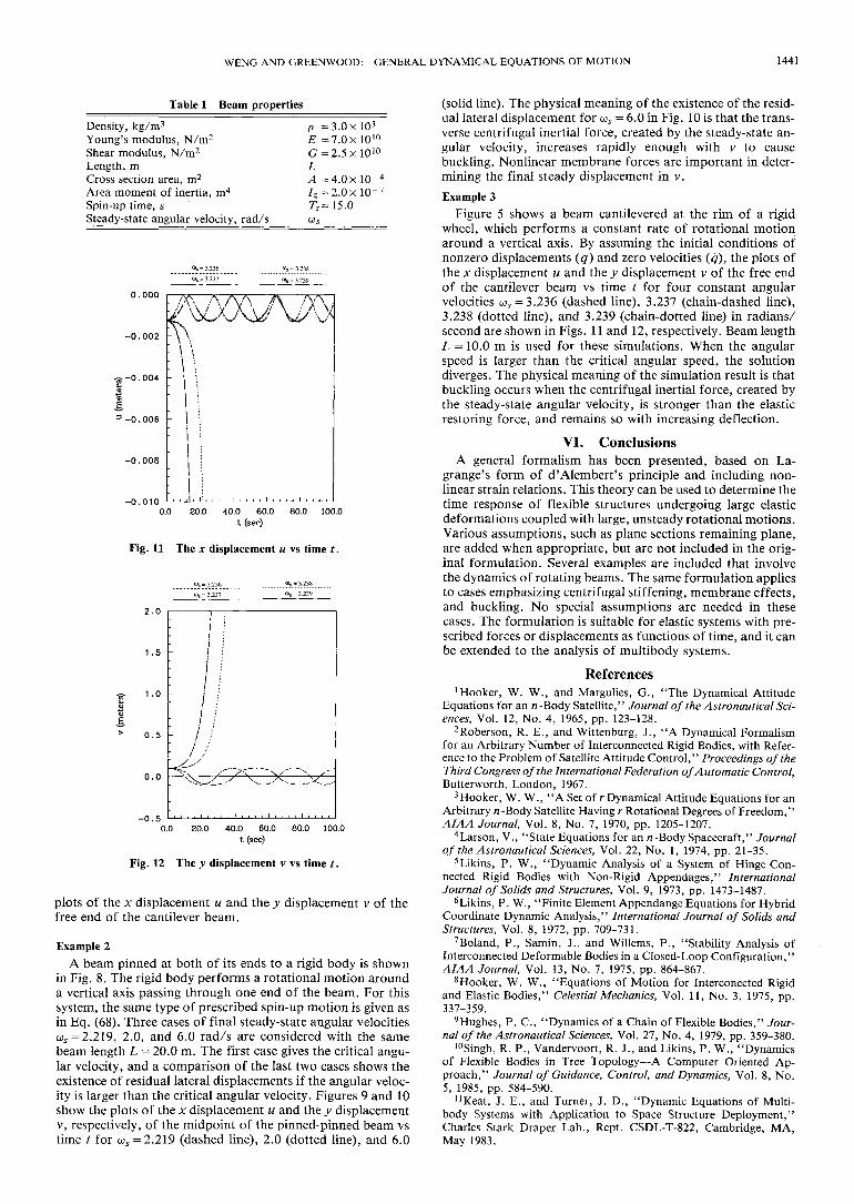
plots of the x displacement u and the y displacement v of thefree end of the cantilever beam.

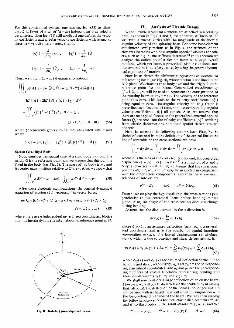
Example 2A beam pinned at both of its ends to a rigid body is shown

in Fig. 8. The rigid body performs a rotational motion arounda vertical axis passing through one end of the beam. For thissystem, the same type of prescribed spin-up motion is given asin Eq. (68). Three cases of final steady-state angular velocities(jos = 2.219, 2.0, and 6.0 rad/s are considered with the samebeam length L = 20.0 m. The first case gives the critical angu-lar velocity, and a comparison of the last two cases shows theexistence of residual lateral displacements if the angular veloc-ity is larger than the critical angular velocity. Figures 9 and 10show the plots of the x displacement u and the y displacementv, respectively, of the midpoint of the pinned-pinned beam vstime t for us = 2.2\9 (dashed line), 2.0 (dotted line), and 6.0

(solid line). The physical meaning of the existence of the resid-ual lateral displacement for co5 = 6.0 in Fig. 10 is that the trans-verse centrifugal inertial force, created by the steady-state an-gular velocity, increases rapidly enough with v to causebuckling. Nonlinear membrane forces are important in deter-mining the final steady displacement in v.Example 3

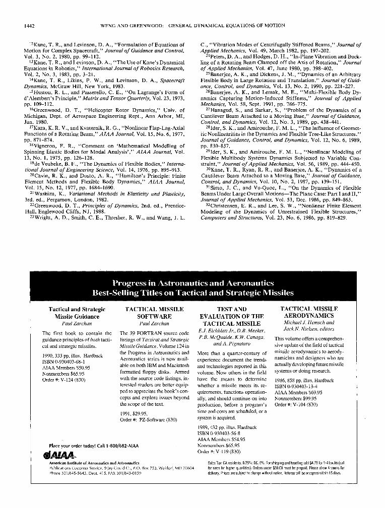
Figure 5 shows a beam cantilevered at the rim of a rigidwheel, which performs a constant rate of rotational motionaround a vertical axis. By assuming the initial conditions ofnonzero displacements (q) and zero velocities (<?), the plots ofthe x displacement u and the y displacement v of the free endof the cantilever beam vs time t for four constant angularvelocities w5 = 3.236 (dashed line), 3.237 (chain-dashed line),3.238 (dotted line), and 3.239 (chain-dotted line) in radians/second are shown in Figs. 11 and 12, respectively. Beam lengthL = 10.0 m is used for these simulations. When the angularspeed is larger than the critical angular speed, the solutiondiverges. The physical meaning of the simulation result is thatbuckling occurs when the centrifugal inertial force, created bythe steady-state angular velocity, is stronger than the elasticrestoring force, and remains so with increasing deflection.

VI. ConclusionsA general formalism has been presented, based on La-

grange's form of d'Alembert's principle and including non-linear strain relations. This theory can be used to determine thetime response of flexible structures undergoing large elasticdeformations coupled with large, unsteady rotational motions.Various assumptions, such as plane sections remaining plane,are added when appropriate, but are not included in the orig-inal formulation. Several examples are included that involvethe dynamics of rotating beams. The same formulation appliesto cases emphasizing centrifugal stiffening, membrane effects,and buckling. No special assumptions are needed in thesecases. The formulation is suitable for elastic systems with pre-scribed forces or displacements as functions of time, and it canbe extended to the analysis of multibody systems.

Referenceslooker, W. W., and Margulies, G., 'The Dynamical Attitude

Equations for an n-Eody Satellite," Journal of the Astronautical Sci-ences, Vol. 12, No. 4, 1965, pp. 123-128.

2Roberson, R. E., and Wittenburg, J., "A Dynamical Formalismfor an Arbitrary Number of Interconnected Rigid Bodies, with Refer-ence to the Problem of Satellite Attitude Control," Proceedings of theThird Congress of the International Federation of Automatic Control,Butterworth, London, 1967.

3Hooker, W. W., "A Set of r Dynamical Attitude Equations for anArbitrary n -Body Satellite Having r Rotational Degrees of Freedom,"AIAA Journal, Vol. 8, No. 7, 1970, pp. 1205-1207.

4Larson, V., "State Equations for an «-Body Spacecraft," Journalof the Astronautical Sciences, Vol. 22, No. 1, 1974, pp. 21-35.

5Likins, P. W., "Dynamic Analysis of a System of Hinge-Con-nected Rigid Bodies with Non-Rigid Appendages," InternationalJournal of Solids and Structures, Vol. 9, 1973, pp. 1473-1487.

6Likins, P. W., "Finite Element Appendange Equations for HybridCoordinate Dynamic Analysis," International Journal of Solids andStructures, Vol. 8, 1972, pp. 709-731.

7Boland, P., Samin, J., and Willems, P., "Stability Analysis ofInterconnected Deformable Bodies in a Closed-Loop Configuration,"AIAA Journal, Vol. 13, No. 7, 1975, pp. 864-867.

8Hooker, W. W., "Equations of Motion for Interconected Rigidand Elastic Bodies," Celestial Mechanics, Vol. 11, No. 3, 1975, pp.337-359.

9Hughes, P. C., "Dynamics of a Chain of Flexible Bodies," Jour-nal of the Astronautical Sciences, Vol. 27, No. 4, 1979, pp. 359-380.

10Singh, R. P., Vandervoort, R. J., and Likins, P. W., "Dynamicsof Flexible Bodies in Tree Topology—A Computer Oriented Ap-proach," Journal of Guidance, Control, and Dynamics, Vol. 8, No.5, 1985, pp. 584-590.

HKeat, J. E., and Turner, J. D., "Dynamic Equations of Multi-body Systems with Application to Space Structure Deployment,"Charles Stark Draper Lab., Rept. CSDL-T-822, Cambridge, MA,May 1983.


12Kane, T. R., and Levinson, D. A., "Formulation of Equations ofMotion for Complex Spacecraft," Journal of Guidance and Control,Vol. 3, No. 2, 1980, pp. 99-112.

13Kane, T. R., and Levinson, D. A., "The Use of Kane's DynamicalEquations in Robotics," International Journal of Robotics Research,Vol. 2, No. 3, 1983, pp. 3-21.

14Kane, T. R., Likins, P. W., and Levinson, D. A., SpacecraftDynamics, McGraw Hill, New York, 1983.

15Huston, R. L., and Passerello, C. E., "On Lagrange's Form ofd'Alembert's Principle," Matrix and Tensor Quarterly, Vol. 23, 1973,pp. 109-112.

16Greenwood, D. T., "Helicopter Rotor Dynamics," Univ. ofMichigan, Dept. of Aerospace Engineering Rept., Ann Arbor, MI,Jan. 1980.

17Kaza, K. R. V., and Kvaternik, R. G., "Nonlinear Flap-Lag-AxialFunctions of a Rotating Beam," AIAA Journal, Vol. 15, No. 6, 1977,pp. 871-874.

18Vigneron, F. R., "Comment on 'Mathematical Modelling ofSpinning Elastic Bodies for Modal Analysis'," AIAA Journal, Vol.13, No. 1, 1975, pp. 126-128.

19de Veubeke, B. F., "The Dynamics of Flexible Bodies," Interna-tional Journal of Engineering Science, Vol. 14, 1976, pp. 895-913.

20Cavin, R. K., and Dusto, A. R., "Hamilton's Principle: FiniteElement Methods and Flexible Body Dynamics," AIAA Journal,Vol. 15, No. 12, 1977, pp. 1684-1690.

21Washizu, K., Variational Methods in Elasticity and Plasticity,3rd. ed., Pergamon, London, 1982.

22Greenwood, D. T., Principles of Dynamics, 2nd. ed., Prentice-Hall, Englewood Cliffs, NJ, 1988.

23Wright, A. D., Smith, C. E., Thresher, R. W., and Wang, J. L.

C., "Vibration Modes of Centrifugally Stiffened Beams," Journal ofApplied Mechanics, Vol. 49, March 1982, pp. 197-202.

24Peters, D. A., and Hodges, D. H., "In-Plane Vibration and Buck-ling of a Rotating Beam Clamped off the Axis of Rotation," Journalof Applied Mechanics, Vol. 47, June 1980, pp. 398-402.

25Banerjee, A. K., and Dickens, J. M., "Dynamics of an ArbitraryFlexible Body in Large Rotation and Translation," Journal of Guid-ance, Control, and Dynamics, Vol. 13, No. 2, 1990, pp. 221-227.

26Banerjee, A. K., and Lemak, M. E., "Multi-Flexible Body Dy-namics Capturing Motion-Induced Stiffness," Journal of AppliedMechanics, Vol. 58, Sept. 1991, pp. 766-775.

27Hanagud, S., and Sarkar, S., "Problem of the Dynamics of aCantilever Beam Attached to a Moving Base," Journal of Guidance,Control, and Dynamics, Vol. 12, No. 3, 1989, pp. 438-441.

28Ider, S. K., and Amirouche, F. M. L., "The Influence of Geomet-ric Nonlinearities in the Dynamics and Flexible Tree-Like Structures,"Journal of Guidance, Control, and Dynamics, Vol. 12, No. 6, 1989,pp. 830-837.

29Ider, S. K., and Amirouche, F. M. L., "Nonlinear Modeling ofFlexible Multibody Systems Dynamics Subjected to Variable Con-straint," Journal of Applied Mechanics, Vol. 56, 1989, pp. 444-450.

30Kane, T. R., Ryan, R. R., and Banerjee, A. K., "Dynamics of aCantilever Beam Attached to a Moving Base," Journal of Guidance,Control, and Dynamics, Vol. 10, No. 2, 1987, pp. 139-151.

31Simo, J. C., and Vu-Quoc, L., "On the Dynamics of FlexibleBeams Under Large Overall Motions—The Plane Case: Part I and II,"Journal of Applied Mechanics, Vol. 53, Dec. 1986, pp. 849-863.

32Christensen, E. R., and Lee, S. W., "Nonlinear Finite ElementModeling of the Dynamics of Unrestrained Flexible Structures,"Computers and Structures, Vol. 23, No. 6, 1986, pp. 819-829.

Progress in Astronautics and AeronauticsBest-Selling Titles on Tactical and Strategic Missiles

Tactical and StrategicMissile Guidance

Paul Zarchan

The first book to contain theguidance principles of both tacti-cal and strategic missiles.

1990, 333 pp,illus, HardbackISBN 0-930403-68-1AIAA Members $50.95Nonmembers $65.95Order #:V-124 (830)

TACTICAL MISSILESOFTWAREPaul Zarchan

The 39 FORTRAN source codelistings of Tactical and StrategicMissile Guidance, Volume 124 inthe Progress in Astronautics andAeronautics series is now avail-able on both IBM and Macintoshformatted floppy disks. Armedwith the source code listings, in-terested readers are better equip-ped to appreciate the book's con-cepts and explore issues beyondthe scope of the text.

1991, $29.95,Order #: PZ-Software (830)

Place your order today! Call 1 -800/682-AIAA

TEST ANDEVALUATION OF THE

TACTICAL MISSILEEJ. Eichblatt Jr., D.B. Meeker,P.B. McQuaide, K.W. Canaga,

and A. Pignataro

More than a quarter-century ofexperience document the trendsand technologies reported in thisvolume. Now others in the fieldhave the means to determinewhether a missile meets its re-quirements, functions operation-ally, and should continue on intoproduction, before a program'stime and costs are scheduled, or asystem is acquired.

1989,432 pp, illus, HardbackISBN 0-930403-56-8AIAA Members $54.95Nonmembers $65.95Order #: V-l 19 (830)

TACTICAL MISSILEAERODYNAMICSMichael J. Hemsch andJack N. Nielsen, editors

This volume offers a comprehen-sive update of the field of tacticalmissile aerodynamics to aerody-namicists and designers who areactually developing future missilesystems or doing research.

1986, 858 pp, illus, HardbackISBN 0-930403-13-4AIAA Members $69.95Nonmembers $99.95Order #: V-104 (830)

American Institute of Aeronautics and AstronauticsPublications Customer Service, 9 Jay Could Ct., P.O. Box 753, Waldorf, MD 20604Phone 301/645-5643, Dept. 415, FAX 301/843-0159

Sales Tax: CA residents, 8.25%; DC, 6%. For shipping and handling add $4.75 for 1-4 books (callfor rates for higher quantities). Orders under $50.00 must be prepaid. Please allow 4 weeks fordelivery. Prices are subject to change without notice. Returns will be accepted within 15 days.

General Dynamical Equations of Motion for Elastic Body Systems

Documents

Transcript of General Dynamical Equations of Motion for Elastic Body Systems