GENERAL ARTICLE The Challenge of Fluid Flow
13
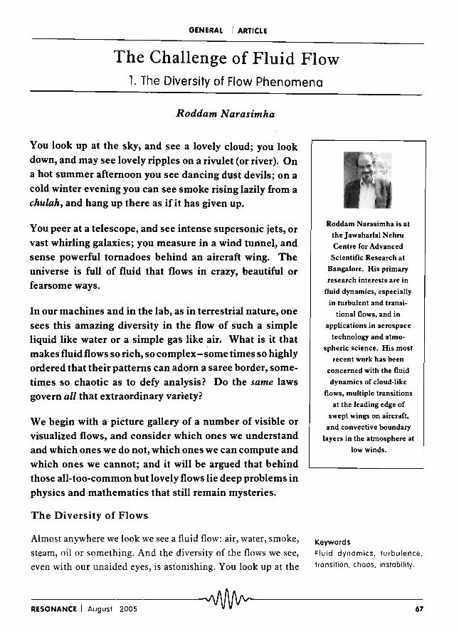
GENERAL I ARTICLE The Challenge of Fluid Flow 1. The Diversity of Flow Phenomena Roddam Narasimha You look up at the sky, and see a lovely cloud; you look down, and may see lovely ripples on a rivulet (or river). On a hot summer afternoon you see dancing dust devils; on a cold winter evening you can see smoke rising lazily from a chulah, and hang up there as if it has given up. You peer at a telescope, and see intense supersonic jets, or vast whirling galaxies; you measure in a wind tunnel, and sense powerful tornadoes behind an aircraft wing. The universe is full of fluid that flows in crazy, beautiful or fearsome ways. In our machines and in the lab, as in terrestrial nature, one sees this amazing diversity in the flow of such a simple liquid like water or a simple gas like air. What is it that makes fluid flows so rich, so complex - some times so highly ordered that their patterns can adorn a saree border, some- times so chaotic as to defy analysis? Do the same laws govern all that extraordinary variety? We begin with a picture gallery of a number of visible or visualized flows, and consider which ones we understand and which ones we do not, which ones we can compute and which ones we cannot; and it will be argued that behind those all-too-common but lovely flows lie deep problems in physics and mathematics that still remain mysteries. The Diversity of Flows Almost anywhere we look we see a fluid flow: air, water, smoke, steam, oil or something. And the diversity of the flows we see, even with our unaided eyes, is astonishing. You look up at the Roddam Narasimha is at the Jawaharlal Nehru Centre for Advanced Scientific Research at Bangalore. His primary research interests are in fluid dynamics, especially in turbulent and transi- tional flows, and in applications in aerospace technology and atmo- spheric science. His most recent work has been concerned with the fluid dynamics of cloud-like flows, multiple transitions at the leading edge of swept wings on aircraft, and convective boundary layers in the atmosphere at low winds. Keywords Fluid dynamics, turbulence, transition, chaos, instability.
Transcript of GENERAL ARTICLE The Challenge of Fluid Flow
GENERAL I ARTICLE
The Challenge of Fluid Flow 1. The Diversity of Flow Phenomena
Roddam Narasimha
You look up at the sky, and see a lovely cloud; you look down, and may see lovely ripples on a rivulet (or river). On a hot summer afternoon you see dancing dust devils; on a cold winter evening you can see smoke rising lazily from a chulah, and hang up there as if it has given up.
You peer at a telescope, and see intense supersonic jets, or vast whirling galaxies; you measure in a wind tunnel, and sense powerful tornadoes behind an aircraft wing. The universe is full of fluid that flows in crazy, beautiful or fearsome ways.
In our machines and in the lab, as in terrestrial nature, one sees this amazing diversity in the flow of such a simple liquid like water or a simple gas like air. What is it that makes fluid flows so rich, so complex - some times so highly ordered that their patterns can adorn a saree border, sometimes so chaotic as to defy analysis? Do the same laws govern all that extraordinary variety?
We begin with a picture gallery of a number of visible or visualized flows, and consider which ones we understand and which ones we do not, which ones we can compute and which ones we cannot; and it will be argued that behind those all-too-common but lovely flows lie deep problems in physics and mathematics that still remain mysteries.
The Diversity of Flows
Almost anywhere we look we see a fluid flow: air, water, smoke,
steam, oil or something. And the diversity of the flows we see,
even with our unaided eyes, is astonishing. You look up at the
Roddam Narasimha is at
the Jawaharlal Nehru
Centre for Advanced
Scientific Research at
Bangalore. His primary
research interests are in
fluid dynamics, especially
in turbulent and transi
tional flows, and in
applications in aerospace
technology and atmo
spheric science. His most
recent work has been
concerned with the fluid
dynamics of cloud-like
flows, multiple transitions
at the leading edge of
swept wings on aircraft,
and convective boundary
layers in the atmosphere at
low winds.
Keywords
Fluid dynamics, turbulence,
transition, chaos, instability.
-R-ES-O-N-A-N-C-E--I-A-U-9-Us-t--2-00-5-------------~-------------------------------6-7

GENERAL I ARTICLE
sky, and may see striking clouds - white, pretty and fluffy
against a perfectly blue sky, or black and threatening against a
gray one. You look down at the ground, and may see a wonderful
medley of ripples, whirlpools, jumps or bores on a tiny rivulet of
water - or on a mighty river. On a hot summer afternoon you can
see dust devils - suddenly twisting themselves into shape pick
ing up all kinds ofloose dirt, and darting wildly around for some
seconds before they flop out. On a cool winter evening you can
see warm smoke rising lazily from a ckulak out in the open, and
hang up there a few metres above ground with no energy left to push into the cooler, heavier air around. You can go to Jog and
keep gazing at the four waterfalls there - majestic, awesome,
graceful, and so different from each other although they are all
making about the same leap.
With the power of modern instrumentation the range of what we
can see goes up enormously. If you peer at a telescope, or the pictures it takes, we can see swirling nebulae whose sizes are
measured in hundreds of thousands of light years. If you have a microscope you can see minute organisms (like spermatozoa, for example) darting here and there in the surrounding medium.
If you can inject smoke and shine laser beams you can see
powerful vortices that would otherwise be invisible in air, such as those that trail behind aircraft. From satellites we can see
cyclones that can wreak havoc. And there can be terrible tsunamis of the kind we experienced in south and south-east
Asia on 26 December 2004. I have put together a collection of some flow pictures of this kind in Figure 1 - I hope you will agree
that they can be crazy, beautiful and fearsome in turn. (A wonderful album compiled by Van Dyke has many others.)
One can go on endlessly like this. This diversity offluid motion
has fascinated man for thousands of years. The Yoga- Viisi~tha
(written perhaps around +6 or 7 c.) uses fluid flow metaphors extensively, and compares the complexity of the human mind
with that of flowing water:
-~------------------------------~------------R-ES-O-N-A-N-C-E-I-A-U-9-US-t-2-0-0-5
GENERAL I ARTICLE
~b )
(1)
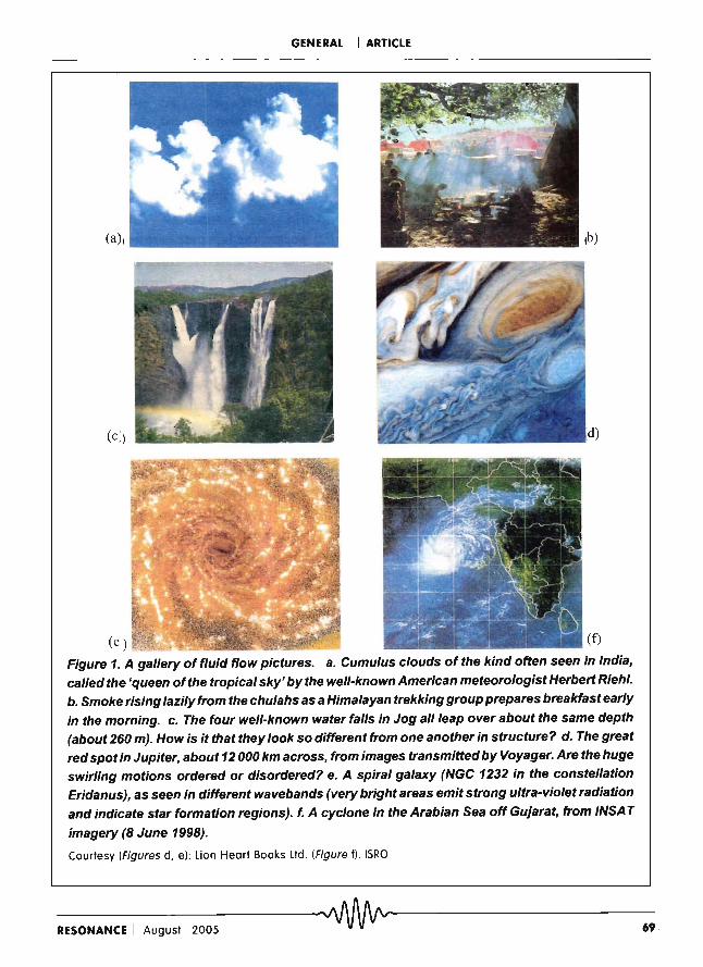
Figure 1. A gallery of fluid flow pictures. a. Cumulus clouds of the kind often seen in India,
called the 'queen of the tropical sky' by the well-known American meteorologist Herbert Riehl. b. Smoke rising lazily from the chulahs as a Himalayan trekking group prepares breakfast early
in the morning. c. The four well-known water falls in Jog all leap over about the same depth (about 260 my. How is it that they look so different from one another in structure? d. The great red spot in Jupiter, about 12 000 km across, from images transmitted by Voyager. Are the huge swirling motions ordered or disordered? e. A spiral galaxy (NGC 1232 in the constellation Eridanus), as seen in different wavebands (very bright areas emit strong ultra-violet radiation
and indicate star formation regions). f. A cyclone in the Arabian Sea off Gujarat, from INSA T
imagery (8 June 1998).
Courtesy (Figures d, el: Lion Heart Books Ltd. (Figure fl: ISRO
--------~~------RESONANCE I August 2005 69

GENERAL I ARTICLE
As water displays itself richly dharQ-ka~ I -Ormi-phe~-~~rfr.
vatho .~alnJa~yate. ' mbhasa,l .. latha vicilra-vihhaw.l
In current, wave, foam and spray, So does the mind exhibit
nanDI". eyall; hi celasab. If A strange, splendid diversity. (3: 110.48)
Figure 2. A Japanese print entitled 'Wind and wave at Awa-Nruto', by Hiroshige Utagawa (1797-1858).
. .
Elsewhere the author sings of the beauty of a whirlpool in
swaying water (iilola-salil'-iivarta-sundari'). And, as if in illustration of Viisi~tha poetry, the Japanese painter Hiroshige Utagawa (1797-1858) catches its essential spirit in a lovely print of Wind and Wave (Figure 2). In renaissance Europe Leonardo da Vinci (1452-1519), who combined within himself the hands and eyes of an engineer as well as an artist, drew wonderfully
faithful pictures of vortices in turbulent water flow.
Do we understand these diverse flows? How many of them can be described by a convincing theory? How many can be computed? After all, isn't the flow of fluids a 'classical' subject, whose governing laws were set down in the first half of the 19th
century? It may be interesting to put together an album of pretty flow pictures, but are there new things to discover? (Answer: yes.) Why do people (like me) spend a life-time investigating fluid flow problems, pursuing the rather esoteric discipline of ' fluid dynamics'?
It is my intention here to try and answer these questions. But before offering answers, we need to look at
those flows and grasp their nature a little better.
Order and Chaos
One of the most striking features of many fluid flows that has fascinated all observers - ancient and modern - is the strange mix of order and chaos that is their characteristic. At one extreme, a flow can be incredibly well-ordered. For example, consider the case of what is called Rayleigh-Benard convection between two large horizontal plates, the lower one of which is warmer
7 -O--------------------------------------------~~----------------R-ES-O-N-A-N-C-E---I-A-U-9U-S-t---20-0-5

GENERAL I ARTICLE
than the upper. If the temperature difference between the plates is sufficiently small there is no flow at all, and heat is transported from the lower to the upper plate through thermal conduction in
the enclosed fluid - which might just as well have been a solid, it would have made no difference. But as the temperature difference exceeds a critical value the fluid suddenly overturns into motion, in a row of highly organized rolls (Figure 3) (or a pattern
of hexagonal cells as seen from the top if the upper surface is free). Those rolls can be so steady in time and so repeatable in
space that they could well decorate a saree border. As the temperature difference increases the rolls get distorted and
begin to sway and list, and eventually break down into chaotic motion. We see one example of such breakdown in the bottom
panels of Figure 3. (But, as we shall see shortly, such apparently chaotic motion may well contain hidden order.)
Saree-border type organization may also be seen in a variety of other situations - most famously in the flow in the wake of a
circular cylinder. (By the principle of Galilean invariance, the relative flow is the same whether the cylinder moves in still fluid
or the fluid flows past a cylinder at rest; so we shall use either frame interchangeably.) In this case, as a critical velocity is
exceeded the flow in the wake spontaneously breaks into two parallel rows of staggered vortices - clockwise in one row, anti
clockwise in the other (Figure 4), forming what is called a Karman vortex street. (See article in current issue.) (We often
'hear' those vortices when power lines sing in wind; the Greeks even had an 'aeolian' harp, whose strings were resonantly
Figure 3. Thermal convection in a box (10:4:1) (lower plate warmer), showing changes from saree-border type ordered motion (top) towards turbulent convection (bottom, box rotating). In the middle picture the temperature differential is higher at the right.
Suggested Reading
[1] J H Arakeri, Bernoulli's
Equation, Resonance,
Vo1.5, No.8, pp.54-71, Au
gust 2000.
[2] J H Arakeri and P N Shan
kar, Ludwig Prandtl and
Boundary Layers in Fluid
Flow, Resonance, Vol.5,
No.12, pp. 48-63, Decem
ber2000.
[3] R Govindarajan , Turbu
lence and Flying Machines,
Resonance, Vol.4, No. 11,
pp.54-62, November 1999.
[4] R Narasimha, Order and
chaos in fluid flows, Curro
Sci., Vol. 56, pp.629-645,
1987.
[5] R Narasimha, Turbulence
on computers, Curro Sci., Vol. 64, pp. 8-32, 1993.
[6] R Narasimha, Divide, con
quer and unify,Nature, Vol.
432, p. 807, 2004.
[7] M Van Dyke, An album of
fluid motion, Parabolic
Press, Stanford, CA, 1982.
________ ,AAAAAA ______ __ RESONANCE I August 2005 v V V V V v 71

Figure 4. Another ordered motion: the Karman vortex street behind a circular cylinder. This staggered arrangement of vortices in
two parallel rows is 'stable'. (See Box 2 on Reynolds number.)
Figure 5. An idealized, schematic picture of how transition from laminar to turbulent flow occurs in the boundary layer on a flat plate, from two-dimen
sional instability through turbulent spots to fully developed turbulent flow. (Reproduced from Frank M White, Viscous Fluid Flow, McGraw-Hili International Editions, 1991).
GENERAL ! ARTICLE
'plucked' by natural wind.) As the velocity is increased further,
the Karman vortex street breaks down into apparent chaos, but
again, it turns out, with hidden order in it.
Instability and Transition to Turbulence
In these and other cases, the appearance of order actually marks
the onset of an instability (Box 1). The critical condition that
sparks this onset is given not so much by a temperature differ
ence or flow velocity, which may be specific to a particular appa
ratus and fluid, as (much more generally) by an appropriate non
dimensional number like the Rayleigh number in convection
and the Reynolds number in flow past bodies. (Boxes 2 and 3).
u ~
u ~
Stable laminar flow
Laminar! ....... t-----Transition length---~ .. I Turbulent
Ret,
-72-------------------------~-------------R-E-SO--N-A-N-C-E-!-A-U-9-u-st--2-0-0-S

GENERAL I ARTICLE
Box 1. Flow Instability
The words stability and instability are used in so many different senses that it is not possible to go into all
of them here. Briefly, the idea in linear stability theory is that a system in a certain state is stable if a small
perturbation made on it decays, unstable if it grows. In some flow systems, a small perturbation may grow
exponentially under certain conditions - e.g. if the relevant non-dimensional number (see Box 2 or 3)
exceeds a critical value. This growth may however soon reach saturation through nonlinear effects.
Consider the Karman vortex street as an example. The arrangement of Figure 4 is stable in the sense that
if any vortex in the system is displaced, the effect of the rest of the vortices is such as to take the perturbed
vortex back to its original position. However, the birth of the vortex street itself is a result of an instability
that occurs at a critical cylinder Reynolds number (see Box 2) of about 48.5. In fact, the Karman vortex
street is best seen as an example of a global fluid-dynamical oscillator, which makes its appearance at the
critical Reynolds number of 48.5. (At this critical value the flow encounters what is known as a bifurcation:
this is a point of structural instability, at which the solution can exhibit a significant qualitative change in
its structure - e.g. from a steady state to an oscillatory state.)
In the boundary layer on a flat plate, as Figure 5 suggests, the flow is laminar and stable to small
perturbations till a critical Reynolds number of about Re = U x Iv = 105 is reached (here x is distance from
the leading edge). Beyond this point sinusoidal disturbances of certain frequencies can grow as they travel
downstream in space, till they reach a point where the boundary layer has grown enough to be no longer
unstable to those frequencies. From then on the disturbance decays. However, the flow is now unstable
to other frequencies, which again can grow in amplitude before they also eventually decay again. On the
whole, disturbance of so~e frequency or other will keep growing beyond the critical point. All these
disturbances travel downstream, so if the original disturbance is a pulse at some point, the disturbance at
that point vanishes eventually but will be present in some form at some downstream location at some later
time. Such an instability is called convective.
In contrast to the Karman vortex street, the boundary layer is best seen as a selective amplifier, in the sense
that the instability waves appear only because there is a forcing somewhere almost always in the
environment. If the environmental disturbance levels are reduced transition to turbulence is delayed; the
best reading of the experimental evidence suggests that the critical Reynolds number is inversely
proportional to the environmental disturbance intensity, and so can increase without limit as the
environment becomes increasingly 'quiet'. There is in this view no such thing as 'natural' transition on a
flat plate, although that phrase is unfortunately still widely used in text books and in engineering practice.
I myself have long been interested in flow past surfaces, such as e.g. an aircraft wing. What happens here in a simple and rather idealized situation is illustrated in Figure S. At a critical distance from the leading edge (more precisely a Reynolds number based
on that distance) instability waves can appear in the flow, and grow downstream; eventually they break down into islands of
-R-ES-O-N-A-N-C-E--I-A-U-9-US-t--2-0-05-------------~~------------------------------n-

GENERAL I ARTICLE
Box 2. The Reynolds Number
Fluid flows are determined by a variety of forces pressure, viscous stresses, gravity (including
buoyancy), surface tension, electro- and ferro-magnetic etc. As it is impossible (and rarely desirable) to
take all of them into account in analysing specific flows, fluid dynamicists identify various non
dimensional groups that give some indication of which among these many forces may be dominant in any
given situation. The grand-father of all such non-dimensional groups is the Reynolds number, named after
the British engineer Osborne Reynolds who first showed the value of the concept in his studies of pipe
flow, treated elsewhere in another box (see Box 4).
The Reynolds number is commonly thought of as a measure of the ratio of inertial to viscous forces. The
inertial force is another name for the effective acceleration of the fluid. Because a fluid is a continuous
medium, all these forces are most conveniently estimated for unit volume of the fluid. It must be
remembered that only estimates of orders of magnitude are involved in forming non-dimensional groups
like the Reynolds number.
As an example, consider the flow of an incompressible fluid of density p and viscosity J1 at a velocity U
past a circular cylinder of diameter D. As velocity changes of order U may be expected to occur over
distances of order D, a characteristic flow time is of order DIU, and a characteristic acceleration of a fluid
element is of order UI(DIU) = eJ2ID. So the inertial force is of order peJ2ID per unit volume. The viscous
stress is typically of order J1 UID, and its spatial rate of change J1 UID2 gives a measure of the viscous
force per unit volume. The ratio of the two is the Reynolds number
Re= pU2
D2 = pUD, == UD D p,U p, II
where it is convenient to introduce V=J1 Ip as the 'kinematic' viscosity (so called because its units, m2/s
in the metric system, do not involve mass).
Note that we could just as well have used the radius of the cylinder (rather than the diameter) in defining
the Reynolds number. In that case the numerical value of the Reynolds number would be half of what is
given above. This only shows that there can be arbitrary numerical constants in defining the Reynolds
number, and when quoting numerical values for it we must clearly state the specific choices for the
quantities that go into it, and stick to those choices. All the more reason why the Reynolds number in one
class of flow (flow past cylinders, e.g.) cannot be directly compared with values in a different class (e.g.
wings). Once a choice is made, however, we can say that a doubling ofthe Reynolds number will double
the inertial force in comparison with viscous forces.
Reynolds numbers vary widely for different flow types - from something like 10-2 for the mote in the
sunbeam to nearly 1012 for a tropical cyclone.
The Reynolds number is a non-dimensional group in the sense that its value will be the same in any
internally consistent system of units - SI, British, etc.
--------~~------74 RESONANCE I August 2005

GENERAL I ARTICLE
chaos called turbulent spots, which themselves grow and propagate downstream till the flow becomes 'fully turbulent'.
What I have described above is the phenomenon of flow transition - from laminar flow (no disorder) to turbulent flow (apparently complete disorder). Such a transition occurs in
virtually every known flow type, often through one or more intermediate stages of instability of one kind or another. In some flows transition is abrupt or 'hard', in others it can be gradual and slow ('soft'). It can even be both: spots can appear suddenly,
but full-time turbulence emerges slowly as spots need time to grow before they cover the surface. If the non-dimensional parameter governing the flow, like a local flow Reynolds number, varies in space (as in Figure 5) or in time (as it does in the upper reaches of our lungs especially if we are breathing hard, say after jogging), the transitional sequence from laminar to turbulent flow may occur in space or in time (or in both).
Box 3. The Rayleigh Number
The Rayleigh number does for free convection what the Reynolds number does for incompressible flows.
Consider the situation illustrated in Figure 3: two horizontal plates separated by a vertical distance h, the
gap being filled with a fluid of characteristic density Po' viscosity J.l.o and temperature To' The flow is now
driven by a temperature difference !1T. As no characteristic flow velocity is explicitly prescribed in the
statement of the problem, it has to be estimated from the other parameters. We do it this way. Thermal
conduction diffuses temperature, the corresponding fluid property being the 'kinematic' diffusivity lCo ( =
ko / Po c, where ko is the thermal conductivity and c the specific heat). Now a characteristic diffusion time
to smear out a temperature difference of !l.T over a distance h is h2/Ko (easily checked dimensionally).
The effective acceleration due to buoyancy force per unit mass is g !l.plpo' - g !l.TITo' where!l.p and !l.T
are the characterislic density fPd temperature differences. So the velocity that develops due to this
'acceleration' over the diffusion titne isg (!1T/T J (h2/lCo) • The corresponding Reynolds number works out
to what is called the Rayleigh number
Ra= gh2aT h =gh3aT. KoTo Vo . ToKoVo
Another non-dimensional group we will run across is the well-known Mach number, the ratio of flow
velocity to the acoustic speed. This ratio provides a measure of the thermodynamic elastic forces operating
in a compressible flow. If the Mach number is small the 'elastic' forces leading to sound propagation are
also relatively small, so the flow behaves as if it is incompressible.
-R-ES-O-N-A-N-C-E--I-A-U-9-US-t--2-00-5-------------~~------------------------------7-5

GENERAL I ARTICLE
Reverse Transition -Turbulent Flow Becoming Laminar
Under certain conditions (e.g. if the local Reynolds number
decreases downstream) a turbulent flow can revert to a laminar state. This indeed happens in our lungs, as the air flows down
from the wind pipe into numerous tiny bronchioles. This reverse transition from disorder to order does not violate the second law
of thermodynamics, because the flows we are discussing are open systems. Some instances of such relaminarization are
illustrated in Figure 6. You can sometimes see it in the evening sky, when a cloud, bubbling up from the ground, seems all of a
sudden to lose its rough edges and bulges out into a smooth bump. This happens when the cloud hits what is called an
'inversion' - a situation where the temperature locally increases with height, rather than decreasing as it most commonly does.
The rising air then becomes heavier than the air above the inversion and subsides, having converted its kinetic energy to
gravitational. This is similar to the chulah smoke mentioned earlier, and one of the pictures in Figure 6 is a laboratory
simulation of this effect.
Figure 6. 'Reverse' transition from turbulent to laminar flow. a (left). Flow comes into coiled tube from top left in a turbulent state (notice how tube is filled with red dye), but leaves in a laminar state (green filament injected at bottom does not spread). b (right). Jet of dyed water flow up in a tank. On the left, the jet starts out laminar, transitions to turbulence. On the right, the turbulent jet so formed reverts to a laminar state as it hits a stabilizing density gradient created by heating the water at the top and making it lighter.
7-6-------------------------------~-------------R-E-SO--N-A-N-C-E-I-A-U-9-u-st--2-0-0-S

GENERAL I ARTICLE
Box 4. Laminar-turbulent Transition
It is a matter of common observation that fluid flow can be in one of two fundamentally different states.
One of them, called laminar, is regular, smooth or ordered, and the other, called turbulent, is irregular,
chaotic, disordered. In steady laminar flow the velocity at any point is either a constant in time, or has
orderly (periodic or related) fluctuations. In turbulent flow the velocity is fundamentally time-dependent,
exhibits no apparent order, has contributions from all frequencies, and has vorticity (.i.e. fluid elements
have local spin). Some typical turbulent traces are shown in Figure 7.
The first scientific study of the transition from laminar to turbulent flow was conducted by Reynolds
(Figure a) in a pipe. He detected turbulent flow by injecting a filament of dye at a point on the centre-line
near the entry to the pipe. If the flow was laminar the dye remained a straight filament along the centre
line. But if the flow were turbulent the dye spread across the pipe colouring the fluid in the whole pipe.
Laminar and turbulent flow can be made out easily in Figure 6.
By experimenting with different fluids in pipes of different diameter, Reynolds discovered that transition
occurred at more or less the same value of what later came to be called the Reynolds number (see Box 2).
(The name was given by the physicist Arnold Sommerfeld.) In Reynolds's own experiments the critical
value of Re, defined as UDlv, where U is the average velocity across the pipe of diameter D, turned out
to be around 2300.
We now know that the situation is not so simple; if great care is taken in reducing environmental distur
bances, flow perturbations, asymmetries, pipe roughness etc., very high transition Reynolds numbers
(multiple of 105) can in fact be obtained. Between fully laminar and fully turbulent states appear travelling
'slugs' of turbulent flow - preceded and followed by laminar flow - called 'flashes' by Reynolds.
As we show elsewhere, there are also conditions when a turbulent flow can revert to a laminar state - a
transition in the reverse direction, often called relaminarization, is therefore also possible.
Figure: Osborne Reynolds demonstrating transition in pipe flow. Inset shows sketches of the nature of the flow in the pipe, as visualized by a filament of dye injected along the centre-line of the pipe. The sketches illustrate laminar flow, turbulent flow, and turbulent 'flashes'. (Reynolds 1883 Phil. Trans. Roy. Soc. 174:935-982. Interestingly, the paper starts with the sentence, 'The
~1!~~~!IIII~~@ results of this investigation have both a practical :::::::.and philosophical aspect' - a thought that cap-
tures the enduring appeal of fluid dynamics.)
-R-ES-O-N-A-N--C-E-I-A-U-9-U-s-t-2-0-0-5-------------~~&-------------------------------n-
GENERAL I ARTICLE
...; ....... ~.....r-,.Jr-
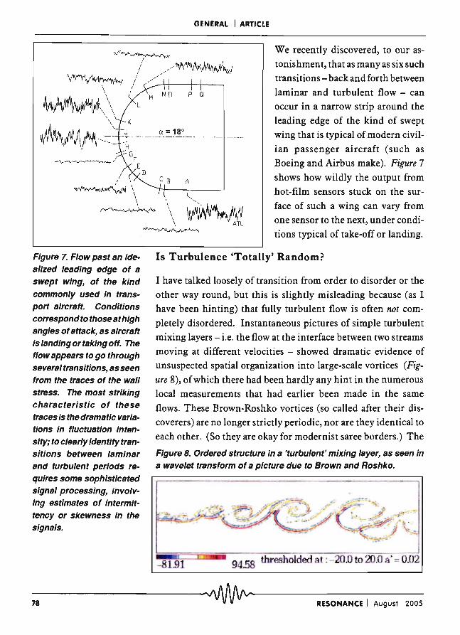
/ . /- 'IIA1'A,"\MVVv~t .. ~ We recently discovered, to our as
tonishment, that as many as six such
transitions - back and forth between
laminar and turbulent flow - can occur in a narrow strip around the
leading edge of the kind of swept
wing that is typical of modern civil
ian passenger aircraft (such as Boeing and Airbus make). Figure 7
shows how wildly the output from
hot-film sensors stuck on the sur
face of such a wing can vary from one sensor to the next, under condi
tions typical of take-off or landing.
Y",-v'\~ I ,// ·W
I /'
\ / //~H---+---+--~
~~\'\ , \
~-~
I I
Figure 7. Flow past an ideal/zed leading edge of a swept wing, of the kind commonly used in transport aircraft. Conditions correspond to those at high angles of attack, as aircraft is landing or taking off. The flow appears to go through several transitions, as seen from the traces of the wall stress. The most striking characteristic of these traces is the dramatic variations in fluctuation intensity; to clearly Identify transitions between laminar and turbulent periods requires some sophisticated signal processing, involving estimates of intermittency or skewness in the signals.
Is Turbulence 'Totally' Random?
I have talked loosely of transition from order to disorder or the other way round, but this is slightly misleading because (as I
have been hinting) that fully turbulent flow is often not com
pletely disordered. Instantaneous pictures of simple turbulent
mixing layers - i.e. the flow at the interface between two streams
moving at different velocities - showed dramatic evidence of unsuspected spatial organization into large-scale vortices (Figure 8), of which there had been hardly any hint in the numerous
local measurements that had earlier been made in the same
flows. These Brown-Roshko vortices (so called after their discoverers) are no longer strictly periodic, nor are they identical to
each other. (So they are okay for modernist saree borders.) The
Figure 8. Ordered structure in a 'turbulent' mixing layer, as seen in a wavelet transform of a picture due to Brown and Roshko.
-78-------------------------------~~-----------R-E-SO--N-A-N-C-E-I-A-U-9-U-S-f-2-0-0-S

GENERAL I ARTICLE
turbulence reveals itself in the jitter and variability that charac
terize these vortices, and in the disordered motion at smaller
scales. So even what is called fully turbulent flow often contains
coherent structures of organized motion within itself.
Let us look at a less obvious example. Figure 9 shows the cross
section of a jet illuminated by a sheet of laser light. (We can
think of it as a slice of flow issuing towards this sheet of paper
from a circular orifice well below.) The fluid coming out of the
orifice is dyed, so the picture shows how this jet fluid is mingling
and mixing with the ambient fluid drawn into the jet. The raw
image on the left - with false colouring indicating dye concen
tration - is what we normally associate with fully turbulent flow.
(Notice by the way all those thin structures in the picture.) The
image on the right is a wavelet transform - a spatial filter that
eliminates both smoother and sharper variations than a speci
fied scale. At the scale chosen, we found that a lobed ring-like
structure pops out, presumably representing a wobbly, azimuth
ally unstable vortex ring. At much smaller scales the wavelet
transform looks random.
In Part 2, we will consider how these phenomena have been
handled, what we can compute and what we can measure, and
where the hard, grand challenges to our understanding lie.
Figure 9. On the left is a
false-colour image of the diametral cross section of a dyed jet (like the one in Figure 6b), taken by laserinduced fluorescence techniques. The flow seems disordered, but a wavelet transform at a suitable scale reveals a fluted ringlike structure - perhaps a lobed vortex ring exhibiting the well-known Wldnall instability, all hidden in the picture on the left.
Address for Correspondence
Roddam Narasimha
Jawaharlal Nehru Centre for
Advanced Scientific Research
Jakkur P.O.
Bangalore 560 064, India.
Email :
roddam@caos .iisc.ernet.in
-R-ES-O-N-A-N-C-E--I-A-U-9-US-t--2-0-05-------------~-------------------------------'-9


![Fluid Flow[1]](https://static.fdocuments.us/doc/165x107/577d38c01a28ab3a6b986b59/fluid-flow1.jpg)